Embed Size (px)
Citation preview

1Quantitative Methods for Economics and Business I
The Simplex Method
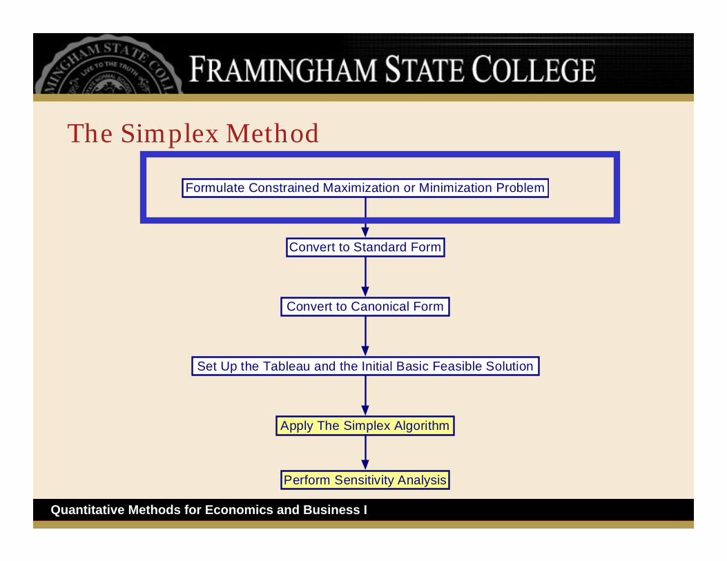
2Quantitative Methods for Economics and Business I
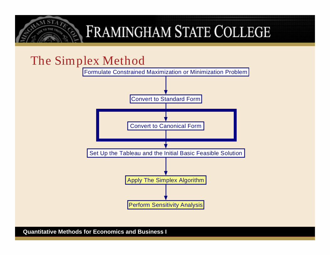
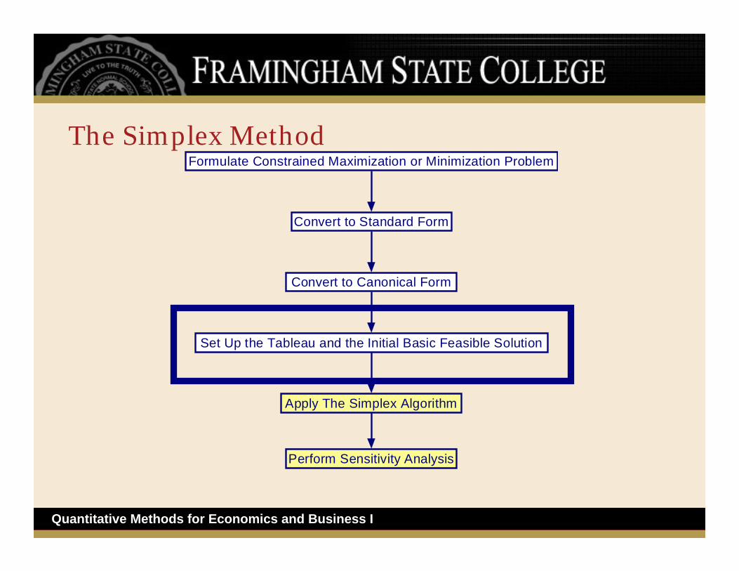
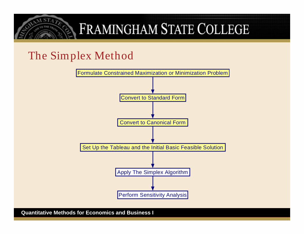
The Simplex Method
Formulate Constrained Maximization or Minimization Problem
Convert to Standard Form
Convert to Canonical Form
Apply The Simplex Algorithm
Perform Sensitivity Analysis
Set Up the Tableau and the Initial Basic Feasible Solution
3Quantitative Methods for Economics and Business I
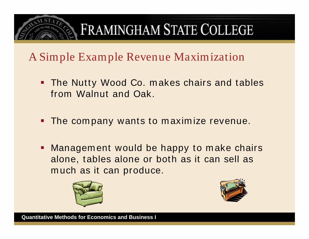
A Simple Example Revenue Maximization
The Nutty Wood Co. makes chairs and tables from Walnut and Oak.
The company wants to maximize revenue.
Management would be happy to make chairs alone, tables alone or both as it can sell as much as it can produce.

4Quantitative Methods for Economics and Business I
Nutty Wood Co. Revenue Maximization cont…
A table sells for $400, needs 5 cubic feet of Walnut and 2.5 cubic feet of Oak.
A chair which takes 2 cubic feet of Oak and 1 cubic foot of Walnut sells for $125.
Only 400 cubic feet of Walnut and only 250 cubic feet of Oak is available.

5Quantitative Methods for Economics and Business I
The Decision Variables
The decision to be made is how many tables and how many chairs to make, so the decision variables are:
Let c be the number of chairs built.
Let t be the number of tables made.
Sales prices are parameters as it is assumed that these are givens.

6Quantitative Methods for Economics and Business I
The Objective Function
What is the objective?
How do we express this in terms of Decision variables c and t?
What is the Objective Function?

7Quantitative Methods for Economics and Business I
The Objective Function
Maximize revenue is the objective.Revenue is Sales Price by Number Sold.Revenue = (125 * c) + (400 * t)So the Objective Function is:
Max Revenue =(125 * c) + (400 * t)
8Quantitative Methods for Economics and Business I
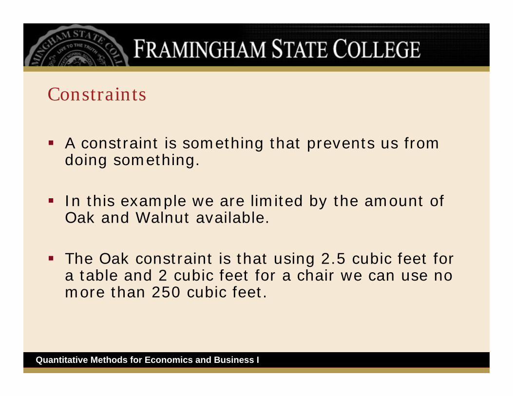
Constraints
A constraint is something that prevents us from doing something.
In this example we are limited by the amount of Oak and Walnut available.
The Oak constraint is that using 2.5 cubic feet for a table and 2 cubic feet for a chair we can use no more than 250 cubic feet.

9Quantitative Methods for Economics and Business I
Constraints cont…
The Walnut constraint is that using 5 cubic feet for a table and 1 cubic foot for a chair we can use no more than 400 cubic feet.
How do we express the constraints mathematically?

10Quantitative Methods for Economics and Business I
Constraints cont…
The Walnut constraint is that using 5 cubic feet for a table and 1 cubic foot for a chair we can use no more than 400 cubic feet.
So:
• (2 * c) + (2.5 * t) 250• (1 * c) + (5 * t) 400
are the constraints.

11Quantitative Methods for Economics and Business I
Bounds on the Problem
Nutty Wood Co. do not make fewer than zero chairs or tables.
How do we express this?
12Quantitative Methods for Economics and Business I
Bounds on the Problem
Nutty Wood Co. do not make fewer than zero chairs or tables.
We express this with lower bounds as follows:
• c 0• t 0
Note this allows for zero in both cases.

13Quantitative Methods for Economics and Business I
Write Down The Full Model

14Quantitative Methods for Economics and Business I
The Model
Maximize 125c + 400t (Revenue)
Subject to 2c + 2.5t 250 (Oak Constraint)
1c + 5t 400 (Walnut Constraint)
c 0 (Lower Bounds)
t 0

15Quantitative Methods for Economics and Business I
The Simplex MethodFormulate Constrained Maximization or Minimization Problem
Convert to Standard Form
Convert to Canonical Form
Apply The Simplex Algorithm
Perform Sensitivity Analysis
Set Up the Tableau and the Initial Basic Feasible Solution

16Quantitative Methods for Economics and Business I
Simple Mathematical Operations on Constraints
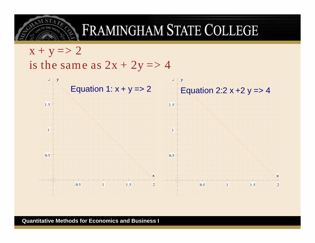
Any constraint may be multiplied or divided through by a positive number without changing the constraint.
• x + y => 2 is the same as 2x + 2y => 4
17Quantitative Methods for Economics and Business I
x + y => 2 is the same as 2x + 2y => 4
0.5 1 1.5 2
0.5
1
1.5
2
x
y
Equation 1: x + y => 2
0.5 1 1.5 2
0.5
1
1.5
2
x
y
Equation 2:2 x +2 y => 4
18Quantitative Methods for Economics and Business I
Simple Mathematical Operations on Constraints
When a “>”, “=>”, “<=“ or “<“ constraint is multiplied or divided through by a negative number, the direction of the constraint must be changed.

19Quantitative Methods for Economics and Business I
Multiply x + y => 2 by -1
(x + y => 2) * (-1) ⇒ -x – y <= -2 and they are equivalent.
0.5 1 1.5 2
0.5
1
1.5
2
x
y
Equation 1: x + y => 2
0.5 1 1.5 2
0.5
1
1.5
2
x
y
Equation 2:- x - y < = -2

20Quantitative Methods for Economics and Business I
Standard Form
A Linear Program is in Standard Form if:
• All the constraints are written as equalities.
• All variables are required to be non-negative.
This involves the addition of “Slack” variables and “Surplus” variables.

21Quantitative Methods for Economics and Business I
Adding Slack Variables
When a Constraint is in the form:
• x + y <= v : With bounds (x => 0, y => 0)
We add a “Slack Variable” to take up the slack between the value of (x + y) and the value of v.
Thus x + y + s = v.
Note that s => 0 since x + y <= v.
22Quantitative Methods for Economics and Business I
Adding Surplus Variables
When a Constraint is in the form:
• x + y => v: With bounds (x => 0, y => 0)
We add a “Surplus Variable” to account for the surplus left over when the value of v is deducted from the values of (x + y).
Thus x + y = v + s
Note that s => 0 since x + y => v.

23Quantitative Methods for Economics and Business I
Adding Surplus Variables cont…
We then shuffle “s” to the left hand side of the equality by subtracting s from both sides, giving:
x + y – s = v
x=> 0, y =>0, and s => 0

24Quantitative Methods for Economics and Business I
Conversion to Standard Form, Nutty Wood Co.
maximize 125c + 400t (Revenue)
Subject to 2c + 2.5t 250 (Oak Constraint) 1c + 5t 400 (Walnut Constraint)
≤≤
c 0 (Lower Bounds) t 0
≥≥

25Quantitative Methods for Economics and Business I
Oak Constraint (1)
This is a “<=” constraint, so we need to add a surplus variable (S1).
1
1
maximize + + (Revenue)125c 400t 0S
Subject to + + 250 (Oak Constraint)2c 2.5t S 1c + 5t 400 (Wal
=≤
1
nut Constraint) c 0 (Lower Bounds) t 0 0S
≥≥≥

26Quantitative Methods for Economics and Business I
Walnut Constraint (2)
This is “<=” constraint, so we need to add a surplus variable (S2).
1 2
1
2
maximize + + + (Revenue)125c 400t 0S 0S
Subject to + + 250 (Oak Constraint)2c 2.5t S 1c + 5t + = 400 (Walnut CoS
=
1 2
nstraint) c 0 (Lower Bounds) t 0 0, 0S S
≥≥≥ ≥

27Quantitative Methods for Economics and Business I
Conventional Presentation
Use x1, x2, x3 etc…in place of c, t, x, y or z.
Slack or Surplus Variables are denoted by:• “S” concatenated with the constraint number
Hence S1 and S3 in the example.

28Quantitative Methods for Economics and Business I
Negative Values on RHS
If any RHS values are negative we multiply through the equality by (-1) to make the RHS value positive.
e.g.
• 2x1 – 3x2 – S = - 12
becomes• -2x1 + 3x2 + S = 12.
29Quantitative Methods for Economics and Business I
The Simplex MethodFormulate Constrained Maximization or Minimization Problem
Convert to Standard Form
Convert to Canonical Form
Apply The Simplex Algorithm
Perform Sensitivity Analysis
Set Up the Tableau and the Initial Basic Feasible Solution

30Quantitative Methods for Economics and Business I
Canonical Form
A Linear Program is in Canonical Form if:
• It is in Standard Form, and
• For each constraint, there exists a variable that appears only in the constraint, and its coefficient in that constraint is “+1”.

31Quantitative Methods for Economics and Business I
Example of Canonical Form
1 2 1 2
1 2 1
1 2 2
maximize + + + (Revenue)125x 400x 0S 0S
Subject to + + 250 (Oak Constraint)2.5x 1S2x + + = 400 (Walnut5x 1S1x
=
1
2
1 2
Constraint) 0 (Lower Bounds)x 0x 0, 0S S
≥≥≥ ≥

32Quantitative Methods for Economics and Business I
Nutty Wood Co. in Full Canonical Form
1 2 1 2
1 2 1
1 2 2
maximize + + + (Revenue)125x 400x 0S 0S
Subject to + + 250 (Oak Constraint)2.5x 1S2x + + = 400 (Walnut5x 1S1x
=
1
2
1 2
Constraint) 0 (Lower Bounds)x 0x 0, 0S S
≥≥≥ ≥
33Quantitative Methods for Economics and Business I
The Simplex MethodFormulate Constrained Maximization or Minimization Problem
Convert to Standard Form
Convert to Canonical Form
Apply The Simplex Algorithm
Perform Sensitivity Analysis
Set Up the Tableau and the Initial Basic Feasible Solution

34Quantitative Methods for Economics and Business I
Setting up The Simplex Tableau
To set up the Simplex Tableau we will:
• Identify the Basic and Non-basic variables.
• Set up a Basic Feasible Solution.
• Look at the form of the Simplex Tableau, and
• Enter the LP and values of the Initial Basic Solution into the Simplex Tableau.

35Quantitative Methods for Economics and Business I
Basic and Non-basic Variables
Recall from the definition of the Canonical Form.
• “For each constraint, there exists a variable that appears only in the constraint, and its coefficient in that constraint is “+1”. “ These variables are the initial Basic Variables.
• The other variables are the Non-basic Variables.

36Quantitative Methods for Economics and Business I
Basic and Non-basic Variables cont…In our example we added S1 and S2 to satisfy the conditions for the Canonical Form. These are the Basic Variables.
The Non-basic Variables are x1 and x2.
1 2 1 2
1 2 1
1 2 2
maximize + + + (Revenue)125x 400x 0S 0S
Subject to + + 250 (Oak Constraint)2.5x 1S2x + + = 400 (Walnut5x 1S1x
=
1
2
1 2
Constraint) 0 (Lower Bounds)x 0x 0, 0S S
≥≥≥ ≥

37Quantitative Methods for Economics and Business I
Setting up the Basic (Feasible) Solution
A Basic Feasible Solution for an LP in the Canonical form is one where:
• The Non-basic variables are set to zero, and
• The Basic variables take on the values of the RHS of their constraint.
38Quantitative Methods for Economics and Business I
Setting up the Basic (Feasible) Solution cont…
A Basic Solution is a Basic Feasible Solution if:
• All of the variables (Basic and Non-basic) are greater than or equal to zero.

39Quantitative Methods for Economics and Business I
The Initial Basic Feasible Solution to Nutty Wood Co.
S1 = 250, S2 = 400.x1 = 0, x2 = 0.The Objective Function Value:• z = 0
1 2 1 2
1 2 1
1 2 2
maximize + + + (Revenue)125x 400x 0S 0S
Subject to + + 250 (Oak Constraint)2.5x 1S2x + + = 400 (Walnut5x 1S1x
=
1
2
1 2
Constraint) 0 (Lower Bounds)x 0x 0, 0S S
≥≥≥ ≥

40Quantitative Methods for Economics and Business I
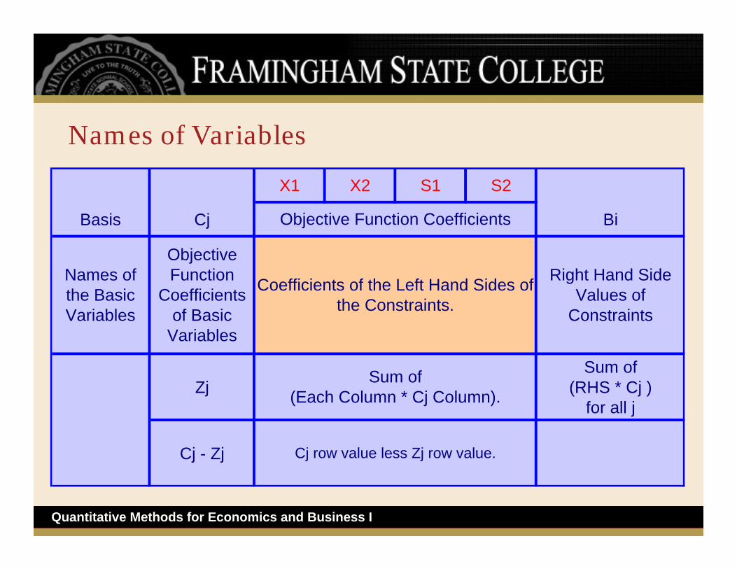
The Form of The Simplex Tableau
Basis Cj Bi
ZjSum of
(RHS * Cj ) for all j
Cj - Zj
Objective Function
Coefficients of Basic
Variables
Names of the Basic Variables
Sum of (Each Column * Cj Column).
Cj row value less Zj row value.
Objective Function Coefficients
Names of the Variables
Coefficients of the Left Hand Sides of the Constraints.
Right Hand Side Values of
Constraints
41Quantitative Methods for Economics and Business I
Names of Variables
X1 X2 S1 S2
Basis Cj Bi
ZjSum of
(RHS * Cj ) for all j
Cj - Zj
Objective Function Coefficients
Coefficients of the Left Hand Sides of the Constraints.
Right Hand Side Values of
Constraints
Objective Function
Coefficients of Basic
Variables
Names of the Basic Variables
Sum of (Each Column * Cj Column).
Cj row value less Zj row value.

42Quantitative Methods for Economics and Business I
Basic Variables
X1 X2 S1 S2
Basis Cj Bi
S1
S2
ZjSum of
(RHS * Cj ) for all j
Cj - Zj
Sum of (Each Column * Cj Column).
Cj row value less Zj row value.
Objective Function Coefficients
Coefficients of the Left Hand Sides of the Constraints.
Right Hand Side Values of
Constraints
Objective Function
Coefficients of Basic
Variables
43Quantitative Methods for Economics and Business I
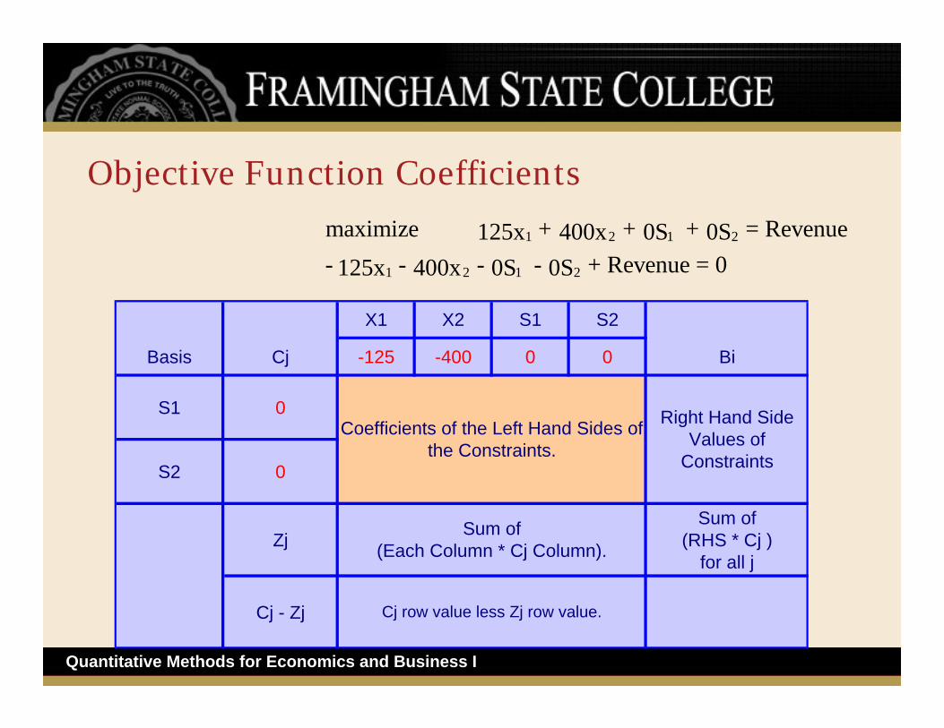
Objective Function Coefficients
1 2 1 2
1 2 1 2
maximize + + + = Revenue125x 400x 0S 0S- - - - + Revenue = 0 125x 400x 0S 0S
X1 X2 S1 S2
Basis Cj -125 -400 0 0 Bi
S1 0
S2 0
ZjSum of
(RHS * Cj ) for all j
Cj - Zj
Right Hand Side Values of
Constraints
Sum of (Each Column * Cj Column).
Cj row value less Zj row value.
Coefficients of the Left Hand Sides of the Constraints.

44Quantitative Methods for Economics and Business I
Coefficients and RHS Values of the Constraints1 2 1
1 2 2
+ + 250 (Oak Constraint)2.5x 1S2x + + = 400 (Walnut Constraint)5x 1S1x
=
X1 X2 S1 S2
Basis Cj -125 -400 0 0 Bi
S1 0 2 2.5 1 0 250
S2 0 1 5 0 1 400
ZjSum of
(RHS * Cj ) for all j
Cj - Zj
Sum of (Each Column * Cj Column).
Cj row value less Zj row value.

45Quantitative Methods for Economics and Business I
The Zj Row
X1 X2 S1 S2
Basis Cj -125 -400 0 0 Bi
S1 0 2 2.5 1 0 250
S2 0 1 5 0 1 400
Zj 0 0 0 0Sum of
(RHS * Cj ) for all j
Cj - Zj Cj row value less Zj row value.
+
=
*
*
46Quantitative Methods for Economics and Business I
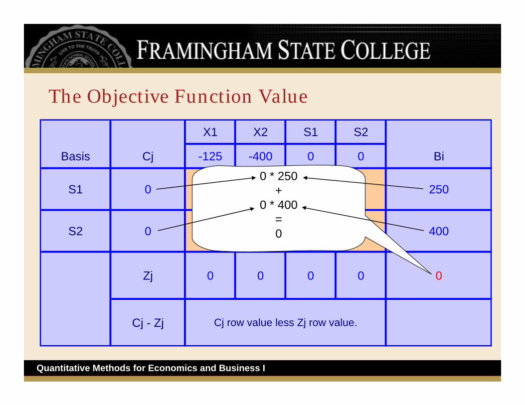
The Objective Function Value
X1 X2 S1 S2
Basis Cj -125 -400 0 0 Bi
S1 0 2 2.5 1 0 250
S2 0 1 5 0 1 400
Zj 0 0 0 0 0
Cj - Zj Cj row value less Zj row value.
0 * 250+
0 * 400=0

47Quantitative Methods for Economics and Business I
The Cj – Zj Row
X1 X2 S1 S2
Basis Cj -125 -400 0 0 Bi
S1 0 2 2.5 1 0 250
S2 0 1 5 0 1 400
Zj 0 0 0 0 0
Cj - Zj -125 - 0= -125
-400 - 0 = -400
0 - 0 = 0
0 - 0 = 0

48Quantitative Methods for Economics and Business I
The Initial Basic Feasible Solution in the Simplex Tableau
X1 X2 S1 S2
Basis Cj -125 -400 0 0 Bi
S1 0 2 2.5 1 0 250
S2 0 1 5 0 1 400
Zj 0 0 0 0 0
Cj - Zj -125 -400 0 0
49Quantitative Methods for Economics and Business I
The Simplex MethodFormulate Constrained Maximization or Minimization Problem
Convert to Standard Form
Convert to Canonical Form
Apply The Simplex Algorithm
Perform Sensitivity Analysis
Set Up the Tableau and the Initial Basic Feasible Solution

50Quantitative Methods for Economics and Business I
The Simplex Algorithm
1. Find the Entering Variable
2. Calculate: By how much can the Entering Variable be increased.
3. Pivot
Variable to Enter?STOP
No
Yes

51Quantitative Methods for Economics and Business I
The Meaning of the Cj, Zj and (Cj – Zj) Rows
Cj value – The gross increase in the Objective Function Value, given a one unit increase in the amount of that variable.
Zj value – The gross decrease in the Objective Function Value, given a one unit increase in the amount of that variable.
Cj-Zj – The net effect on the Objective Function Value of a one unit increase in the amount of that variable.

52Quantitative Methods for Economics and Business I
Find the Entering VariableIn a maximization we want to increase the Objective Function Value as much as possible, so:
Select the variable for which the net effect is the greatest
In our example, (-400) is largest (Cj-Zj), so x2 is the Entering Variable.
Zj 0 0 0 0 0
Cj - Zj -125 -400 0 0

53Quantitative Methods for Economics and Business I
Which row has the smallest quotient X2/Bi?
250/2.5 = 100
400/5 = 80
So S2 will be the variable leaving the basis since the smallest quotient is 80.
X2
Basis Cj -400 Bi
S1 0 2.5 250
S2 0 5 400
Zj 0 0
Cj - Zj -400

54Quantitative Methods for Economics and Business I
Pivoting
Calculate New Row to Replace Pivot Row
Calculate Other Rows in New Tableau
Replace Leaving Variable with Entering Variable in the Basis Column
Update the Objective Function Coefficient for the Entering Variable
Calculate new Zj Values for Each Column
Calculate New (Cj - Zj) Values for Each Column

55Quantitative Methods for Economics and Business I
X1 X2 S1 S2
Basis Cj -125 -400 0 0 Bi
S1 0 2 2.5 1 0 250
S2 0 1 5 0 1 400
Zj 0 0 0 0 0
Cj - Zj -125 -400 0 0
Pivot Row, Column and Element

56Quantitative Methods for Economics and Business I
Calculate “New Row” to Replace Pivot Row
Divide the pivot row by the pivot element:-X1 X2 S1 S2
Basis Cj -125 -400 0 0 Bi
S1 0 2 2.5 1 0 250
S2 0 1 / 5=1/5
5 / 5 = 1
0 / 5=0
1 / 5=1/5
400 / 5=80
Zj 0
Cj - Zj
57Quantitative Methods for Economics and Business I
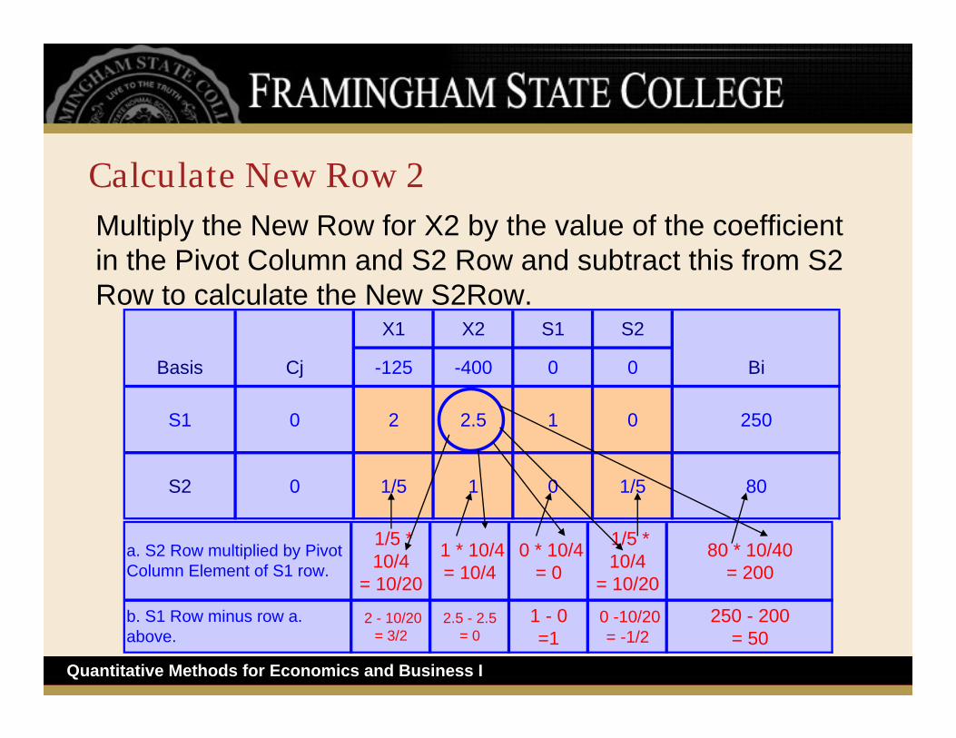
1/5 * 10/4
= 10/20
1 * 10/4= 10/4
0 * 10/4= 0
1/5 * 10/4
= 10/20
80 * 10/40= 200
2 - 10/20= 3/2
2.5 - 2.5= 0
1 - 0=1
0 -10/20= -1/2
250 - 200= 50
a. S2 Row multiplied by Pivot Column Element of S1 row.
b. S1 Row minus row a. above.
Calculate New Row 2Multiply the New Row for X2 by the value of the coefficient in the Pivot Column and S2 Row and subtract this from S2 Row to calculate the New S2Row.
X1 X2 S1 S2
Basis Cj -125 -400 0 0 Bi
S1 0 2 2.5 1 0 250
S2 0 1/5 1 0 1/5 80

58Quantitative Methods for Economics and Business I
X1 X2 S1 S2
Basis Cj -125 -400 0 0 Bi
S1 0 3/2 0 1 -1/2 50
S2 0 1/5 1 0 1/5 80
Zj 0
Cj - Zj
Replace Row2 Basic Variable with Entering Variable
Also check that the result is in Canonical form. If not review Leaving Variable.

59Quantitative Methods for Economics and Business I
Enter X2’s Coefficient From the Objective Function in Cj Column, Row 2
X1 X2 S1 S2
Basis Cj -125 -400 0 0 Bi
S1 0 3/2 0 1 -1/2 50
X2 -400 1/5 1 0 1/5 80
Zj 0
Cj - Zj
60Quantitative Methods for Economics and Business I
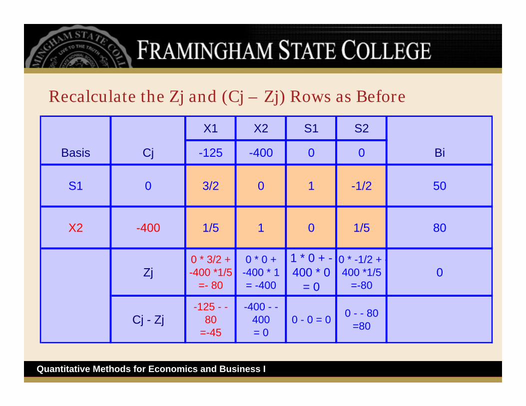
Recalculate the Zj and (Cj – Zj) Rows as Before
X1 X2 S1 S2
Basis Cj -125 -400 0 0 Bi
S1 0 3/2 0 1 -1/2 50
X2 -400 1/5 1 0 1/5 80
Zj0 * 3/2 + -400 *1/5
=- 80
0 * 0 + -400 * 1 = -400
1 * 0 + -400 * 0
= 0
0 * -1/2 + -400 *1/5
=-800
Cj - Zj-125 - -
80=-45
-400 - -400 = 0
0 - 0 = 0 0 - - 80=80
61Quantitative Methods for Economics and Business I
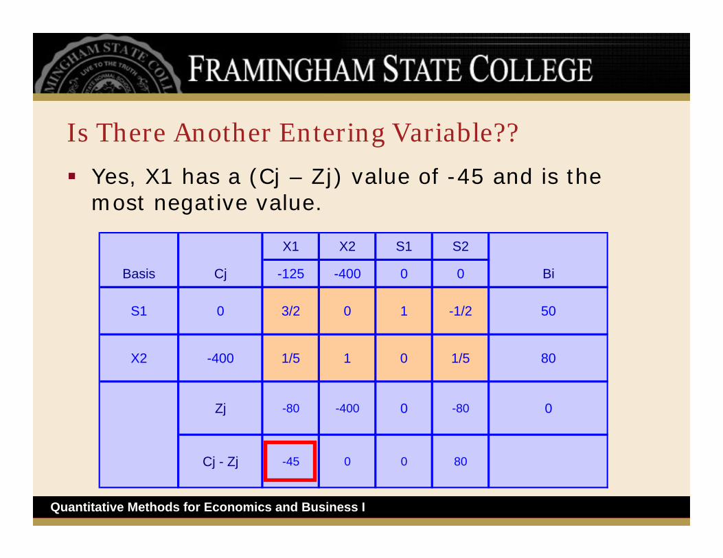
Is There Another Entering Variable??
Yes, X1 has a (Cj – Zj) value of -45 and is the most negative value.
X1 X2 S1 S2
Basis Cj -125 -400 0 0 Bi
S1 0 3/2 0 1 -1/2 50
X2 -400 1/5 1 0 1/5 80
Zj -80 -400 0 -80 0
Cj - Zj -45 0 0 80

62Quantitative Methods for Economics and Business I
Which row has the smallest quotient X2/Bi?
50/(3/2) = 33.33
80/(1/5) = 400
So S1 will be the variable leaving the basis since the smallest quotient is 33.33.
X1
Basis Cj -125 Bi
S1 0 3/2/
50
X2 -400 1/5 / 80
Zj -80 0
Cj - Zj -45

63Quantitative Methods for Economics and Business I
Calculate “New Row” (*) to Replace Pivot Row
Divide the pivot row by the pivot element:-
X1 X2 S1 S2
Basis Cj -125 -400 0 0 Bi
S1 0 3/2 / 3/2
0 / 3/2
1 / 3/2
-1/2 / 3/2
50 / 3/2
X2 -400 1/5 1 0 1/5 80
Zj -80 -400 0 -80 0
Cj - Zj -45 0 0 80

64Quantitative Methods for Economics and Business I
Calculate “New Row” (*) to Replace Pivot Row
X1 X2 S1 S2
Basis Cj -125 -400 0 0 Bi
S1 0 1 0 2/3 -1/3 33.33
X2 -400 1/5 1 0 1/5 80
Zj -80 -400 0 -80 0
Cj - Zj -45 0 0 80

65Quantitative Methods for Economics and Business I
Calculate New Row 2Multiply the New Row by the value of the coefficient in the Pivot Column and Row 2 and subtract this from Row 2 to calculate the New Row 2.
X1 X2 S1 S2
Basis Cj -125 -400 0 0 Bi
S1 0 1 0 2/3 -1/3 33.33
X2 -400 1/5 1 0 1/5 80
1 * 1/5= 1/5
0 * 1/5= 0
2/3 * 1/5
= 2/15
-1/3 * 1/5
= -1/15
100/3 * 1/5= 100/15 = 6.67
1/5 - 1/5= 0
1 - 0= 1
0 - 2/15=-2/15
3/15 - -1/15
= 4/15
80 - 100/15= 73.33
a. S1 Row multiplied by Pivot Column Element of X2 row.
b. X2 Row minus row a. above.

66Quantitative Methods for Economics and Business I
Recalculate the Zj and (Cj – Zj) Rows as Before
X1 X2 S1 S2
Basis Cj -125 -400 0 0 Bi
X1 -125 1 0 2/3 -1/3 33.33
X2 -400 0 1 -2/15 4/15 73.33
Zj-125 * 1 + -400 * 0 =
-125
-125 * 0 + -400 * 1
= -400
(-125*2/3) + (-400 * -
2/15) = -30
(-125 * -1/3) + (-
400 * 4/15)= - 65
(-125*33.33) + (-400*73.33)=
-33,500
Cj - Zj -125 - - 125 = 0
-400 - - 400 = 0
0 - - 30 = 30
0 - -65= 65

67Quantitative Methods for Economics and Business I
Recalculate the Zj and (Cj – Zj) Rows as Before
All (Cj-Zj) values are positive so no entering variable…All Bi are positive...
X1 X2 S1 S2
Basis Cj -125 -400 0 0 Bi
X1 -125 1 0 2/3 -1/3 33.33
X2 -400 0 1 -2/15 4/15 73.33
Zj -125 -400 -30 -65 -33,500
Cj - Zj 0 0 30 65

68Quantitative Methods for Economics and Business I
Recalculate the Zj and (Cj – Zj) Rows as Before
We have a solution we can read from the TableauX1 number of chairs = 33.33X2 number of tables = 73.33Revenue = $33,500S1 = 0 , S2 = 0 : They are Non-Basic and Non-Basic Variableshave value zero!
X1 X2 S1 S2
Basis Cj -125 -400 0 0 Bi
X1 -125 1 0 2/3 -1/3 33.33
X2 -400 0 1 -2/15 4/15 73.33
Zj -125 -400 -30 -65 -33,500
Cj - Zj 0 0 30 65