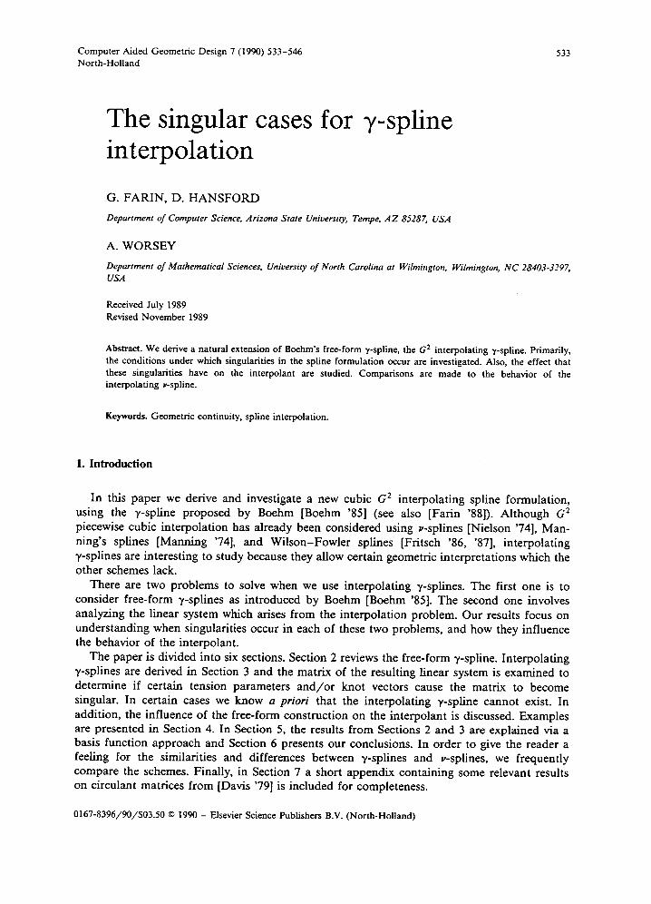
Computer Aided Geometric Design 7 (1990) 533-546

North-Holland 533

The singular cases interpolation

for y-spline

G. FARIN, D. HANSFORD

Department of Computer Science, Arizona State University, Tempe, AZ a-5287, USA

A. WORSEY

Department of Mathematical Sciences, University of North Carolina at Wilmington. Wilmingion, NC 28403-3297, USA

Received July 1989

Revised November 1989

Abstract. We derive a natural extension of Boehm’s free-form y-spline, the G* interpolating y-spline. Primarily,

the conditions under which singularities in the spline formulation occur are investigated. Also, the effect that

these singularities have on the interpolant are studied. Comparisons are made to the behavior of the

interpolating v-spline.

Keywords. Geometric continuity, spline interpolation.

1. Introduction

In this paper we derive and investigate a new cubic G* interpolating spline formulation, using the y-spline proposed by Boehm [Boehm ‘851 (see also [Farin ‘881). Although G*

piecewise cubic interpolation has already been considered using v-splines [Nielson ‘741, Man- ning’s splines [Manning ‘741, and Wilson-Fowler splines [Fritsch ‘86, ‘871, interpolating

y-splines are interesting to study because they allow certain geometric interpretations which the other schemes lack.

There are two problems to solve when we use interpolating y-splines. The first one is to consider free-form y-splines as introduced by Boehm [Boehm ‘851. The second one involves analyzing the linear system which arises from the interpolation problem. Our results focus on understanding when singularities occur in each of these two problems, and how they influence the behavior of the interpolant.

The paper is divided into six sections. Section 2 reviews the free-form y-spline. Interpolating y-splines are derived in Section 3 and the matrix of the resulting linear system is examined to determine if certain tension parameters and/or knot vectors cause the matrix to become singular. In certain cases we know a priori that the interpolating y-spline cannot exist. In

addition, the influence of the free-form construction on the interpolant is discussed. Examples are presented in Section 4. In Section 5, the results from Sections 2 and 3 are explained via a basis function approach and Section 6 presents our conclusions. In order to give the reader a feeling for the similarities and differences between y-splines and v-splines, we frequently compare the schemes. Finally, in Section 7 a short appendix containing some relevant results on circulant matrices from [Davis ‘791 is included for completeness.

0167-8396/90/%03.50 0 1990 - Elsevier Science Publishers B.V. (North-Holland)

534 G. Farin et al. / y-&dine inrerpoldon

Throughout the paper we use boldface characters to denote points and vectors, { - ) denotes an indexed set of values, and (.) denotes such a set when the elements are nondecreasing.

2. Free-form y-splines

Boehm [Boehm ‘851 used the idea behind the design-oriented direct G2 spline of Farin [Farin ‘821 to develop a new G2 free form spline called the y-spline. The y-spline can be directly related to the C2 B-spline in its structure, thus lending itself to theoretical study (unlike the direct G2 spline). The P-spline [Barsky ‘811 has been shown to also have a structure similar to B-splines, however y-splines have the advantage of utilizing the Bernstein-BCzier form. (The /3-spline is a special case of the y-spline: uniform y values and a uniform knot vector.)

Suppose we want to construct a C ’ B-spline. First of all, the de Boor polygon and an associated knot vector is needed. Given this information, we can then construct the points that are used to represent the curve in BCzier form. To adjust the shape of this curve by changing the BCzier points, Farin showed [Farin ‘821 that in order for the curve to be at least G2, the BCzier points must satisfy particular geometric conditions. Boehm used these conditions to develop the y-spline, and the yi determine how to move the Btzier points. Intuitively, the y

values are associated with the control points, but actually they are associated with the knots. So y-splines give us shape handles for moving the Bezier points such that we retain G2 continuity.

Also, in some sense, the y, describe the deviation of the GZ curve from being C2. Not all G2 piecewise cubits possess a y-spline representation (see [Farin ‘88, p. 1611). This is

also the case for P-splines. We shall see later that this fact may cause problems in an

interpolation context. We now formulate an algorithm for open y-spline curves: given a control polygon { di}yL,+’ ,,

a knot sequence u = ( uO, . . . , u,), and a set of parameters ( yi};r,‘, find the piecewise BCzier

polygon of the corresponding y-spline curve. We proceed by first determining the inner Btzier points b,;+r and then find the junction points b,;.

For the inner BCzier points we have:

b3i+l YiAi = S_di_1 +

y;-lAi-2 + Ai-

1 1 s,_, di9

hi+, = Ai + Yi+,At+, d, + YiAi-1

Si 1 Si di+l

where

8i-1 =yi-rAi-z + Ai- + YiAi,

ai=yiAi_r +Ai+yi+rAi+r,

A, = ui+t - ui.

For the junction points we find

'i ‘i-1 ‘3i= Ai_* +Aib3i-l+ Ai_l +Aib3i+l

for i = 1,. . . , n - 1. In order to interpolate to the endpoints it is easiest to set

b,,=d_l, 6, =d,, b3,p1 = d,, b,, =dn+,-

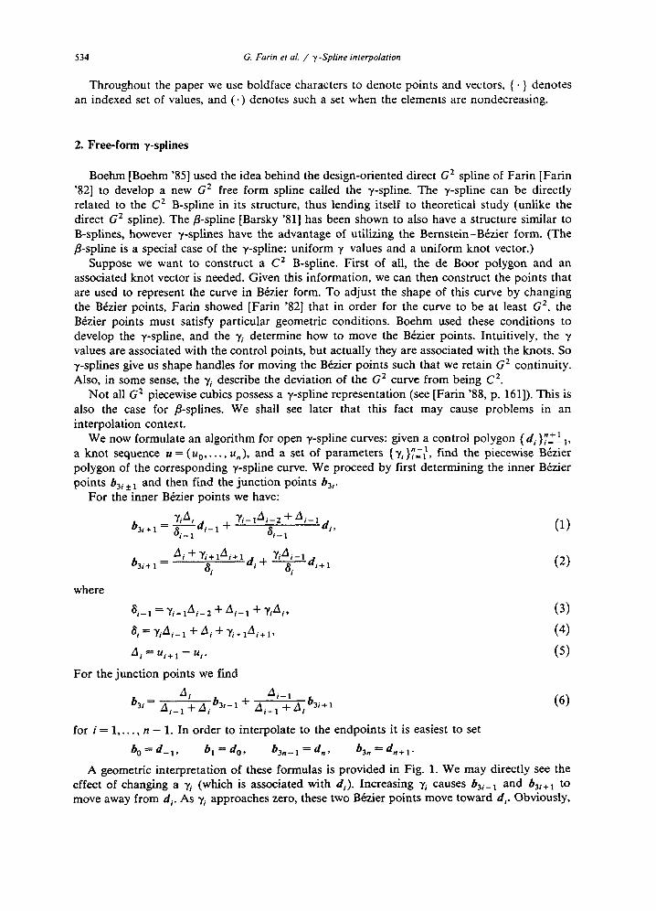
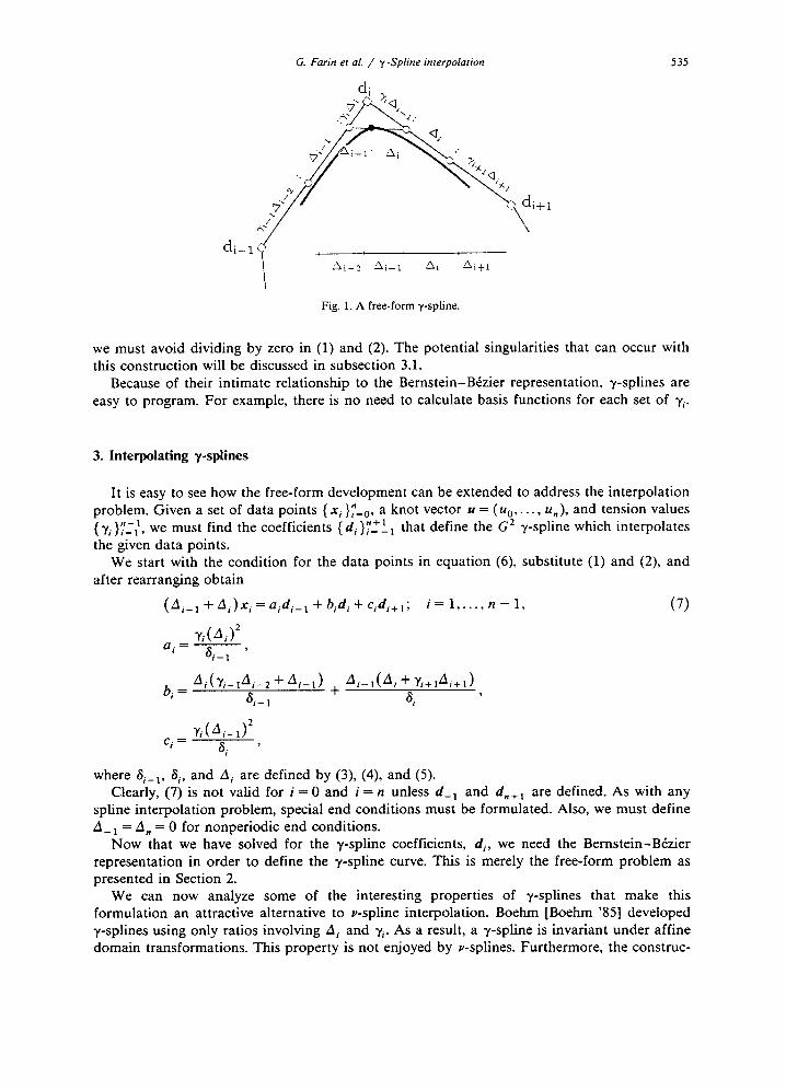
A geometric interpretation of these formulas is provided in Fig. 1. We may directly see the effect of changing a yi (which is associated with di). Increasing yi causes b3i_1 and b3i+, to move away from di. As y, approaches zero, these two Bezier points move toward di. Obviously,

G. Farin et al. / y -Sphe interpolation 535

di-1 : ! : Ai-2 Ai- A, A,+,

Fig. 1. A free-form y-spline.

we must avoid dividing by zero in (1) and (2). The potential singularities that can occur with this construction will be discussed in subsection 3.1.

Because of their intimate relationship to the Bernstein-BCzier representation, y-splines are easy to program. For example, there is no need to calculate basis functions for each set of y,.

3. Interpolating y-splines

It is easy to see how the free-form development can be extended to address the interpolation problem. Given a set of data points ( xi}~_,,, a knot vector IJ = (no,. . . , u,,), and tension values { yj}yzt’, we must find the coefficients { di}:zi 1 that define the G* y-spline which interpolates the given data points.

We start with the condition for the data points in equation (6) substitute (1) and (2) and after rearranging obtain

(A,_l+A,)x,=a,di_l+bid,+cid,+,; i=l,...,n-1, (7)

, YiW2 a.=6i_l’

b, = Ai(Y,-,Ai-2 +Ai_l)

‘i-l +

c, = YiCAi-l12 I si ’

where Si_i. ai, and Ai are defined by (3), (4), and (5). Clearly, (7) is not valid for i = 0 and i = n unless d_, and dntl are defined. As with any

spline interpolation problem, special end conditions must be formulated. Also, we must define A _ , = A,, = 0 for nonperiodic end conditions.

Now that we have solved for the y-spline coefficients, d;, we need the Bernstein-Btzier representation in order to define the y-spline curve. This is merely the free-form problem as presented in Section 2.

We can now analyze some of the interesting properties of y-splines that make this formulation an attractive alternative to v-spline interpolation. Boehm [Boehm ‘SS] developed y-splines using only ratios involving Ai and yi. As a result, a y-spline is invariant under affine domain transformations. This property is not enjoyed by v-splines. Furthermore, the construc-

536 G. Farin et al. / y -Spline interpolation

tion of a y-spline interpolant is based solely on points. Unlike v-splines, it does not involve tangent uecturs. (Tangent vectors tend to be more difficult to work with since they depend on the knot vector and always need to be scaled.) This means that the linear system arising from y-spline interpolation is of a special kind; the matrix is stochastic. That is, the sum of the elements in any row must be 1.

Since the inverse of a stochastic matrix is stochastic, it follows that the de Boor points d,

must be barycentric combinations of the data points xi. However, these combinations need not be convex and typically the de Boor polygon does in fact lie outside the convex hull of the data points.

We now turn to consider under what conditions it is not possible to construct an interpola- tory y-spline.

3.1. Geometric analysis of the singularities

From (1) and (2) the construction of the free-form curve involved divisions which may result in singularities. In our derivation of the interpolating spline we used those very equations, thus carrying over the potential singularities and this issue needs to be examined.

We always assume that the knot sequence is increasing, thus by choosing negative values of y, it is possible for ai_., or 6, to become zero. Simple algebra allows us to determine such instances, however the geometry as we approach these singularities is of more interest.

A closer look at equations (1) and (2) reveals that we cannot construct an interpolant if any two subsequent y, are related by the condition Si = 0 or

Ai = -yiAi-1 -Yi+*‘i+l*

Geometrically, this condition implies that

ratio( di, bji+, , bsi+z) = -YiAi-,/A,

and

ratio(&+t, bJi+z, d;+,) = -Ai/yiA;_l.

A simple geometric argument shows that these two conditions imply either

di+di+t and bji+t. b3i+Z are infinite

or

di=di+, and b3i+,r b3i+2 are finite.

The first situation corresponds to a singularity in the free-form scheme: for given finite d;, the Bezier points bJi+ 1, bji+ 2 tend to infinity as yi, yi+ 1 approach their critical values (causing

ai = 0). The second situation relates to the interpolation problem when the di have to be de-

termined. As y,, y,+, approach their critical values, di and di+ , approach the same finite point,

thus making the constructions (1) and (2) impossible. The limit interpolation curve (for y, having critical values) stays finite, yet has no y-spline representation. It does, however, have a v-spline representation in general, as can be seen from an example in Section 4.

As another interesting example of the interplay between interpolating and free-form y-splines,

consider the case of two subsequent yi, yi+i tending to infinity at the same rate. In the free

form case, this means b3i+ 1 = b,i + 2. In the interpolation case, it produces a row of zeroes in the

coefficient matrix. As a consequence, di + 00 (in general) and b3,+, = b,i+z. The curve is finite and therefore the v-spline exists in general. An exception to this is with symmetric data with periodic ends in which the d, remain finite (the augmented matrix has the same rank as the right-hand side). (This exception can also occur with ‘lucky’ data with clamped ends.) Note

that bsi,, = b3i+2 implies zero curvature at bJi and b3i+3.

G. Fahnn et al. / y-Spline interpolation 537

3.2. Eigenvalue analysis of singularities

Whenever we set up a square linear system, it is necessary to determine if the matrix involved is nonsingular. Since we have incorporated variable parameters, namely the knot

vector and a set of y values, we are not guaranteed a solution as with the interpolating C* B-spline. It is easy to verify that for nonnegative finite y, we are assured a solution since the

knot sequence is assumed to be increasing. In particular, we have a diagonally dominant matrix. Unfortunately, eigenvalue analysis of these matrices is difficult except for very special

instances. Furthermore, when the eigenvalue analysis becomes difficult, it is often less expen- sive to merely try to invert the matrix rather than carry out the complex analysis. For this reason, in subsection 3.2.1 we consider only a simple special case in order to give the reader some indication of the variables that the eigenvalue analysis involves.

As it happens, when we approach y, values that cause the matrix to have a zero eigenvalue, we always get one of two configurations. Most commonly, for y, and y, + , approaching critical values the d,, dicl, f~+~, and bjj+* all tend to infinity. The result is an unbounded curve. Due to the uniqueness of polynomial interpolation, the v-spline also must result in an infinite curve. An example of this behavior is given in Section 4.

Sometimes a critical y,, y,+ 1 pair is chosen so that not only do we have a matrix with a zero eigenvalue, but a singularity also comes from the fact that 8, = 0. In this case, the behavior of

the curve is dictated by the latter type of singularity as discussed in subsection 3.1. This is because generating the system is clearly affected by the condition 8, = 0. Since this singularity is a result of a y-spline representation problem, the v-spline will exist in general.

Let us now look at a special case where the eigenvalue analysis is relatively easy.

3.2.1. Uniform knots, uniform y, and periodic end conditions

We are given n + 1 data points {x, }yeO, a uniform knot vector where Ai = A for all i, and a set of y, = y for all i. (Assume Si # 0.) Equation (7) defined n - 1 equations for our linear system. However, two further equations are generated by the periodic end conditions and so the final system is (n + 1) X (n + 1). Since y-splines are invariant under affine domain transforma- tions, we may assume that A = 1 and so finding the interpolant amounts to solving

2(y+I) Y

1:

Y d0 r,

Y 2(u+I) Y d, r1

= . 9

Y qY+l) ; * . 4-I r n-l

Y Y 2(~+1)__ d, _ _ m _

(8)

with ‘; = 2(2y + 1)x,; i = 0,. . ., n. The matrix in this linear system is a circulant matrix (see Section 7) and the eigenvalues are

~j=2(y+1)+ycos(Bj)+ycos(nBj) (9)

with Bj = 2nj/( n + 1).

(It is necessary to use the identity eie = cos(8) + i sin(@), and the fact that the eigenvalues of a real symmetric matrix are real.) Consequently, the interpolation problem has a unique solution if and only if

-2 yf 2+cos(o,) +cos(n/j,) ’ ‘=O’ l”mo’no (10)

538 G. Farin er al. / y-Spike interpolation

Taking i = 0, it follows that choosing y = -l/2 always produces a singular matrix and so the interpolation problem has no unique solution in this case. (As it happens, this y also causes a 6, = 0 singularity.) In addition, it should be observed that the singular values depend critically upon the precise value of n. For example, the choice y = - 1 produces a zero eigenvalue if and only if n is even.

Since a diagonally dominant matrix is non-singular, the interpolation problem can be ill-defined only if y < - l/2. Consequently, we shall focus on dealing with negative ‘tension’ parameters. We should note that Nielson [Nielson’ 741 did experiment with the negative ‘tension’ parameters that are associated with the v-spline.

An interesting geometric phenomenon occurs for values of y close to - l/2. Namely, the de

Boor points tend toward the barycenter of the data points. This is explained by the following observations. The choice y = -l/2 is the onb one for which the elements in any row of the matrix sum to zero. From the result of the lemma in Section 7 it follows that in this case all

cofactors are equal. (Although irrelevant to this discussion, we point out that a simple inductive proof can be used to show that, in particular, A,, = (n + l).) Now, since the determinant of a matrix is a continuous function of its elements, it follows from Cramer’s rule that as y tends to -l/2 the elements of the inverse matrix must all tend to the same value. That this value is (n + 1) follows from the observation that the linear system is stochastic. (Of course this same type of behavior can occur in other cases with nonuniform knots and/or y, however due to the symmetry we get this very interesting behavior.)

The behavior of, the interpolant in the neighborhood of all other singularities is entirely different from this and is just as the first configuration was explained in subsection 3.2. In all

of those cases, the de Boor points move outwards as we tend toward the singular value of y and then come back towards the data points when y has passed over the singularity. As mentioned

in subsection 3.2 the Btzier points also tend to infinity causing a curve that tends to infinity.

4. Examples

In this section we present examples to illustrate the singularities that can arise in y-spline

interpolation.

4. I. Case I

In the following example we use uniform y, uniform A = 1, and periodic end conditions. Although simple, this is a useful example because the curves are easily traced and it demon-

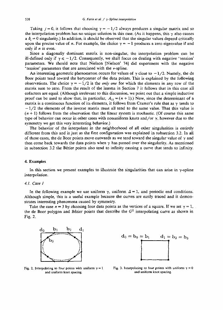
strates interesting phenomena caused by symmetry. Take the case n = 3 by choosing four data points as the vertices of a square. If we set y = 1,

the de Boor polygon and BCzier points that describe the G2 interpolating curve as shown in

Fig. 2.

Fig. 2. Interpolating to four points with uniform y = 1 and uniform knot spacing.

Fig. 3. Interpolating to four points with uniform y = 0 and uniform knot spacing.

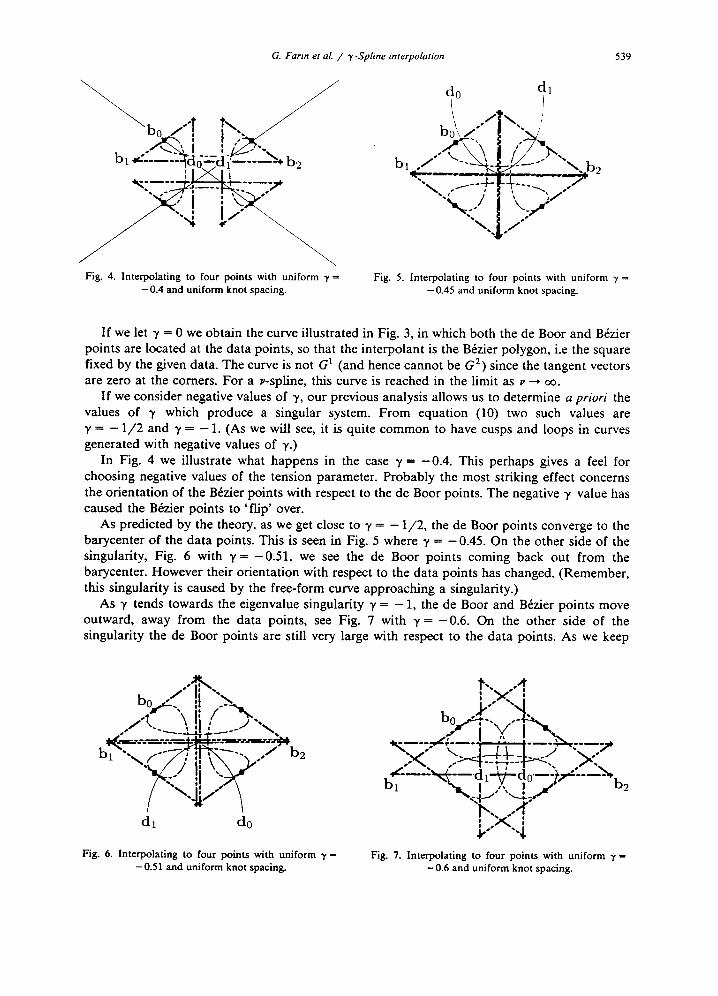
G. Farin et al. / y-Splint- inrerpolarion 539

Fig. 4. Interpolating to four points with uniform y =

- 0.4 and uniform knot spacing.

Fig. 5. Interpolating to four points with uniform y = - 0.45 and uniform knot spacing.

If we let y = 0 we obtain the curve illustrated in Fig. 3, in which both the de Boor and Bezier points are located at the data points, so that the interpolant is the BCzier polygon, i.e the square

fixed by the given data. The curve is not G’ (and hence cannot be G2) since the tangent vectors are zero at the comers. For a v-spline, this curve is reached in the limit as Y --f co.

If we consider negative values of y, our previous analysis allows us to determine u priori the values of y which produce a singular system. From equation (10) two such values are y= -l/2 and y= - 1. (As we will see, it is quite common to have cusps and loops in curves generated with negative values of y.)

In Fig. 4 we illustrate what happens in the case y = -0.4. This perhaps gives a feel for choosing negative values of the tension parameter. Probably the most striking effect concerns the orientation of the BCzier points with respect to the de Boor points. The negative y value has caused the Btzier points to ‘flip’ over.

As predicted by the theory, as we get close to y = - l/2, the de Boor points converge to the barycenter of the data points. This is seen in Fig. 5 where y = -0.45. On the other side of the singularity, Fig. 6 with y = -0.51, we see the de Boor points coming back out from the barycenter. However their orientation with respect to the data points has changed. (Remember, this singularity is caused by the free-form curve approaching a singularity.)

As y tends towards the eigenvalue singularity y = - 1, the de Boor and BCzier points move

outward, away from the data points, see Fig. 7 with y = -0.6. On the other side of the singularity the de Boor points are still very large with respect to the data points. As we keep

dl do

Fig. 6. Interpolating to four points with uniform y =

- 0.51 and uniform knot spacing. Fig. 7. Interpolating to four points with uniform y =

- 0.6 and uniform knot spacing.

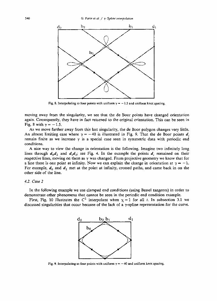
540 G. Farin et al. / y -SpIme interpolation

do b2 bl

Fig. 8. Interpolating to four points with uniform y = - 1.5 and uniform knot spacing.

moving away from the singularity, we see that the de Boor points have changed orientation again. Consequently, they have in fact returned to the original orientation. This can be seen in Fig. 8 with y = - 1.5.

As we move farther away from this last singularity, the de Boor polygon changes very little. An almost limiting case where y = -40 is illustrated in Fig. 9. That the de Boor points di

remain finite as we increase y is a special case seen in symmetric data with periodic end conditions.

A nice way to view the change in orientation is the following. Imagine two infinitely long lines through d,d, and d,d,; see Fig. 4. In the example the points di remained on their respective lines, moving on them as y was changed. From projective geometry we know that for a line there is one point at infinity. Now we can explain the change in orientation at y = - 1. For example, do and d, met at the point at infinity, crossed paths, and came back in on the other side of the line.

4.2. Case 2

In the following example we use clamped end conditions (using Bessel tangents) in order to demonstrate other phenomena that cannot be seen in the periodic end condition example.

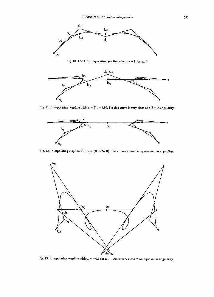
First, Fig. 10 illustrates the C2 interpolant when y, = 1 for all i. In subsection 3.1 we discussed singularities that occur because of the lack of a y-spline representation for the curve.

do b2 bl dl

Fig. 9. Interpolating to four points with uniform y = -40 and uniform knot spacing.

G. Farin et al. / y-Spline interpolation 541

Fig. 10. The Cz interpolating y-spline where y, = 1 for all i.

-+-

Fig. 11. Interpolating y-spline with y, = (1, - 1.99.1): this curve is very close to a 6 = 0 singularity.

Fig. 12. Interpolating v-spiine with pi = (0, -24,O); this curve cannot be represented as a y-sptine.

Fig. 13. Interpolating y-spline with yi = -0.9 for all i; this is very close to an eigenvalue singularity.

542 G. Farin et al. / y Spline inrerpohon

In Fig. 11 we see the set of y, = (1, - 1.99, l} is close to such a singular case. As the theory predicted, two Sj + 0 cause the associated d, to move toward a common point, leaving the b,

finite. If we convert the y, at this singularity (where - 1.99 is replaced by - 2) to Y-spline

tension values Y; = (0, - 24,0}, we see as in Fig. 12 that the v-spline does exist, and indeed this singularity is merely a y-spline representation problem. (A conversion formula for y-splines

and v-splines is given in [Boehm ‘851.) Through direct means, we find that y, = - 1 for all i results in a zero eigenvalue. In Fig. 13

we see that as we approach this value with y, = { -0.9, - 0.9, - 0.9} the y-spline coefficients di

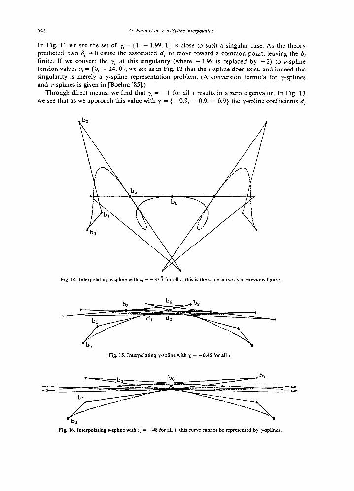
Fig. 14. Interpolating v-spline with vi = -33.7 for all i; this is the same curve as in previous figure.

Fig. 15. Interpolating y-spline with yi = -0.45 for all i.

Fig. 16. Interpolating v-spline with vi = - 48 for all i; this curve cannot be represented by y-splines.

G. Farin et al. / y Spline interpolation 543

are getting very large and, importantly, so are the b,. Converting this y value to a Y, we see in Fig. 14 that the v-spline curve with Y, = { - 33.5, - 33.7, - 33.7) is also becoming unbounded.

This is just as was predicted in subsection 3.2. Our final example comes from choosing a value of y that produces both an eigenvalue

singularity and a 6 singularity. It happens that y, = -l/2 for all i not only causes a 6 = 0 singularity but also causes a zero eigenvalue. In Fig. 15 we see that as we approach this singularity with y, = -0.45 for all i we get the same type of behavior as seen in Fig. 11. The curve in the limit does remain finite. Indeed, by examining Fig. 16 with the corresponding v-spline at this singularity with vi = -48 for all i, the curve does exist.

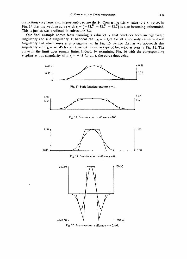
Fig. 17. Basis function: uniform y = 1.

0.50 0.50

O”jO i O.jO Fig. 18. Basis function: uniform y = 100.

Fig. 19. Basis function: uniform y = 0.

250.50

-249.50

250.50

-249.50

Fig. 20. Basis function: uniform y = - 0.499.

544

5. The basis functions

G. Farin et al. / y-Spline interpolation

As mentioned previously, the fact that y-splines are closely related to B-splines allows for an in-depth theoretical analysis. Boehm [Boehm ‘851 demonstrated the construction of the basis

functions (also called the y-B-splines) and they are given further attention by Farm [Farin ‘881 and Luscher [Luscher ‘891. The basis functions were created such that they have the properties of partition of unity, positivity, and local support. Prehaps the most interesting aspect of the construction of the y-spline basis functions is that their graph is only C’ (not G’), but by taking linear combinations of them we obtain a G2 curve.

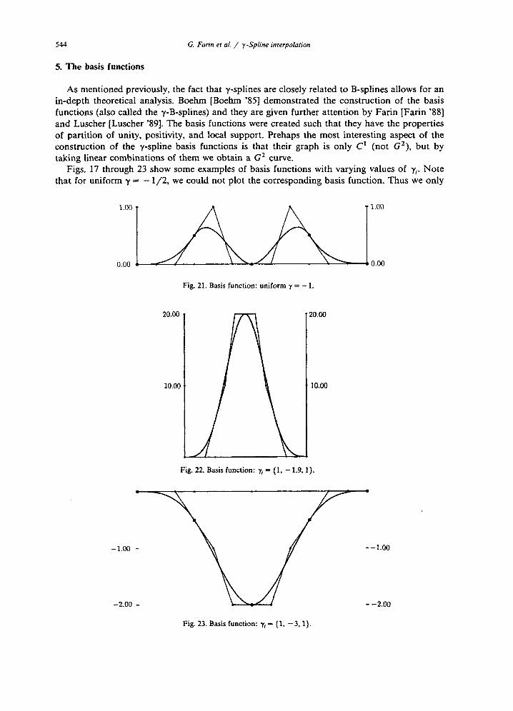
Figs. 17 through 23 show some examples of basis functions with varying values of yi. Note

that for uniform y = - l/2, we could not plot the corresponding basis function. Thus we only

Fig. 21. Basis function: uniform y = - 1.

-1.00 -

Fig. 22. Basis function: yi = (1, - 1.9,l).

Fig. 23. Basis function: -y, = (1, - 3.1).

G. Farin et al. / y Spline interpolation 545

show y = - 0.499 in Fig. 20. Although singularities occur in the linear system for y = - 1, we

have no problem plotting the basis function of the associated free-form curve in Fig. 21. Note how the basis functions ‘flip over’ as yZ goes through a singularity at yZ = - 2.

6. Conclusions

We have developed interpolating y-splines and have seen that they may fail to solve the interpolation problem for two different reasons: singularities may occur due to zero eigenvalues of the coefficient matrix or to inconsistencies in the geometry of the control polygon.

By comparison, v-splines only exhibit the first kind of singularities. They, on the other hand, are (in our experience) awkward to handle because of the dependence of the v-values on the

parametrization. Future G* interpolation schemes may (hopefully) provide automatic ways for selecting the

shape parameters. We feel that y-splines would be inadequate for that purpose: the selection of shape parameters will most likely be an iterative process. If we change the set of shape parameters slightly, we should expect only a slight change in the resulting new control polygon. This is guaranteed with the v-spline approach, but not with the y-spline approach nor with interpolating fl-splines, for that matter.

7. Appendix: Circulant matrices

Although Davis [Davis ‘791 offers a complete introduction to the theory of circulant matrices, we include here some basic definitions and results that are used in the analysis of the y-spline interpolation problem.

Consider a generic circulant matrix C of order n + 1. That is, a square matrix of the form:

c, ci . . . c, \ c, co . . . c,_i

C=circ(c,, ci ,..., C”) = . . . . . . . . . . . Cl c* . . . co /

Let II=circ(O, 1,0 ,..., 0). Then circ(c,, c ,,.._, c,)=c,Z+c,l7+ -.. +c,,ZI”-‘. Thus C is circulant if and only if we may write C =p(II) for some polynomial p(z). We associate with the n-tuple o = (c,, ci, . . . , c,,) the polynomial

p,(z)=c,+c,z+ *** +c,zn,

which is known as the representer of the circulant [Davis ‘791. Using the change of variable z = eie, p, becomes

#(0) =+m(B) =c,+c, e”+ ... +c, eine (11)

which, for our purposes, is more useful as the representer of C. The point to introducing & is that it gives us a closed form expression for the eigenvalues Xj

of c, viz:

xj=+u s ; ( 1 j=O, 1 ,..., n.

This important result is used in subsection 3.2.1, as is the although straightforward, is new.

Lemma. Let C = cifc( co, c,, . _ . , c,) be a circulant matrix in Then a/l cofactors of C are equal.

02) following technical lemma which,

which c,+c,+c,+ **- +c,=O.

546 G. Farin er al. / y-Splint- inrerpolnrion

Proof. We first note that in the follo,wing argument all subscripts must be computed using mod(n + 1) arithmetic. This simplifies the notation.

Let Aij (0 < i, j Q n) be the cofactor of C obtained by deleting row (i + 1) and column (j f 1) from C and calculating the determinant of the resulting n X n matrix. The row deleted

from C is the vector

(c_;, c*-,,...,cj-i,...,c,-i).

For any k E (0, 1,. . . , n}, k # i, we can add all other rows of A,j to the row

(c- k> C1-kv.**9Cj-k,o**, h-k),

without changing its value. If we do this it follows, since ce + c, + * . - +c, = 0, that the row

may be written as

( -c_i, - c*_i ,..., - cj_i ,..., - c,_i).

Modulo a sign change, this is tantamount to permuting rows (k + 1) and (i + 1) in the original matrix C and so, almost by definition, the result follows. 0

Acknowledgements

This research was supported in part by NSF grant DMC-8807747 and by DOE grant DE-FGO2-87ER25041 to Arizona State University and by NSF grant DMS-8803257 to the University of North Carolina at Wilmington. As always, Robert Barnhill was both helpful and supportive. Appreciated suggestions were provided by Wolfgang Boehm and Tony DeRose.

References

Barsky, B. (1981). The Beta-spline: a local representation based on shape parameters and fundamental geometric

measures. Ph.D. Thesis, Dept. of Computer Science, University of Utah.

Boehm, W. (1985). Curvature continuous curves and surfaces. Computer Aided Geometric Design 2 (2). 313-323.

Davis, P. (1979). Circulunt Murrices, Wiley, New York.

Farin, G. (1982). Visually C2 cubic sptines, Computer Aided Design 14 (3). 137-139.

Fat-in, G. (1988), Curves and Surfaces for Computer Aided Geometric Design, Academic Press, New York.

Fritsch, F. (1986). The Wilson-Fowler sphne is a r-sphne, Computer Aided Geometric Design 3 (2). 155-162.

Fritsch, F. (1987). Energy comparison of Wilson-Fowler sptines with other interpolating sphnes, in: G. Farin, ed.,

Geometric Modeling: Algorithms and New Trends, SIAM, Philadelphia, PA, 185-202.

Luscher, N. (1989), A Greville-like formula for y-B-spline functions, Computer Aided Geometric Design 6 (2).

173-176.

Manning, J.R. (1974), Continuity conditions for spline curves, Computer J. 17, 181-186. Nielson, G. (1974), Some piecewise polynomial alternatives to sptines under tension, in: R.E. Barnhill and R.F.

Riesenfeld, eds., Computer Aided Geometric Design, Academic Press, New York, 209-235.