Embed Size (px)
Citation preview
Regional Science and Urban Economics 35 (2005) 756–776
www.elsevier.com/locate/econbase
The size distribution of Chinese cities
Gordon Andersona,T, Ying Geb
aDepartment of Economics, University of Toronto, 150 St. George Street, Toronto, Ontario, Canada M5S 3G7bSchool of International Trade and Economics, University of International Business and Economics,
Beijing 100029, P.R. China
Received 28 November 2004
Available online 19 February 2005
Abstract
This paper uses urban data to investigate two important issues regarding city sizes in China, the
relative growth of cities and the nature of the city size distribution. The manner in which cities of
different sizes grow relative to each other is examined and, contrary to the common empirical finding
that the relative size and rank of cities remains stable over time, it is found that the Economic
Reforms and the One Child Policy since 1979 have delivered significant structural change in the
Chinese urban system. The city size distribution remains stable before the reforms but exhibits a
convergent growth pattern in the post-reform period. The theoretical literature on city sizes highlights
a link between log normal and Pareto distributions for city sizes prompting the employment of
Pearson goodness-of-fit tests to examine directly which theoretical distribution provides the best
approximation to the empirical city size distribution. Contrary to the evidence for other countries, a
log normal rather than Pareto specification turns out to be the preferred distribution.
D 2005 Elsevier B.V. All rights reserved.
JEL classification: C24; R12
Keywords: Zipf’s law; Gibrat’s law; Convergence
1. Introduction
Two questions have been of long-standing interest to urban economists: the first
concerns how cities of different sizes grow relative to each other, the second concerns
0166-0462/$ -
doi:10.1016/j.r
T Correspond
E-mail add
see front matter D 2005 Elsevier B.V. All rights reserved.
egsciurbeco.2005.01.003
ing author. Tel.: +1 416 978 4620; fax: +1 416 978 6713.
resses: [email protected] (G. Anderson)8 [email protected] (Y. Ge).
G. Anderson, Y. Ge / Regional Science and Urban Economics 35 (2005) 756–776 757
which theoretical distribution provides the best approximation for the empirical city size
distribution. Regarding the former question, most empirical studies suggest that the
relative size and rank of cities remain stable over time. Eaton and Eckstein (1997) favored
a parallel growth pattern over divergent or convergent growth patterns for French and
Japanese cities. Black and Henderson (1999) constructed a theoretical model to explain the
parallel growth rates of cities and found support for this pattern in data on U.S. cities.
Overman and Ioannides (2001) developed a stochastic transition kernel for the evolution
of the distribution of U.S. metropolitan area populations from 1900 to 1990 and produced
results suggesting persistence in the city size distribution. Dobkins and Ioannides (2000)
studied the dynamic evolution of the city size distribution in U.S. and confirmed that the
city growth in U.S. is relatively stable over time. Sharma (2003) found that the growth of
cities in India may be parallel in the long-run but with short-run deviations from the long-
term pattern.
With respect to the second question, the dominating view in the literature is that the
Pareto distribution fits best. The idea, mentioned as early as Auerbach (1913), was
propagated by Zipf (1949) who claimed that not only does the size distribution of cities
follow a Pareto law, but also the distribution has a shape parameter of 1. In empirical
studies, when cities are ordered by population size, regressing the logarithm of their rank
on the logarithm of their size yields a slope coefficient close to minus one in so many
instances that the phenomena has acquired the status of the eponymous Zipf’s law. Taking
exponents, the relationship can be seen to be a special case of a power rule relating the
size rank of a city to some power of its population size rendering the statistical distribution
appropriate for the relationship a member of the family due to Pareto (1897) more
commonly employed in modeling income distributions. More generally, the Pareto
exponents generated from the rank size regression are not necessarily equal to unity, and
this so-called brank size ruleQ is believed to be applicable to almost all countries around
world. Rosen and Resnick (1980) estimated the Pareto exponent for 44 countries. Their
estimates ranged from 0.81 to 1.96, with a sample mean of 1.14. Soo (in press)
investigated a new data set of 75 countries and found the average value of Pareto
exponent is 1.1, which is significantly greater than 1 predicted by Zipf’s law. The rank
size regression has also been extended to test the validity of the Pareto specification.
Ioannides and Overman (2003) used a nonparametric procedure to estimate Gibrat’s law
for city growth processes and their results favored Zip’s law. The rank size rule emerged
from regularly observed features of the data and lacked any economic theoretic
foundation. Recently, Gabaix and Ioannides (2004) outlined economic urban agglomer-
ation models by Gabaix (1999), Cordoba (2003), Rossi-Hansberg and Wright (2004) each
of which, under various assumptions about city size shocks, deliver Zipf’s law. Duranton
(2002) embeds a quality ladder model of growth in an urban framework, it does not
produce Zipf’s law but it does produce simulations that are well approximated by a log
normal distribution.
This paper exploits Chinese data to investigate these two general issues regarding the
city size distribution. There are three reasons why the experience of China is of interest.
First, most empirical studies in this topic focus on the developed countries and, as a
developing country with the largest population and a rapid urbanization process, China
provides a bnon-developedQ comparison case. Secondly, over the last 30 years, China has
G. Anderson, Y. Ge / Regional Science and Urban Economics 35 (2005) 756–776758
experienced substantial economic and social reforms including a transition toward a
market economy where human capital flows more freely, integration into the world
economy where access to foreign markets matters and the introduction of bThe One ChildPolicyQ which changed the structure of random shocks that city sizes are subject to.
Whether such fundamental reforms induced changes in the city size distributions is of
interest. Thirdly, China has experienced very rapid urbanization process since 1980, with
the development of a large number of new cities. This is significantly different from the
stable city growth processes in most countries, where the main channel of urban growth is
the expansion of existing cities rather than the birth of new ones. Indeed a critical element
of the Gabaix (1999) argument is that the rate of growth in the number of cities does not
exceed the population growth rate and it is instructive to observe the consequences for the
theory when this condition is not met.
This paper draws two substantive conclusions. First, in examining the evolution of the
Chinese urban system over time, it finds that economic reforms engendered a structural
change in the city size distribution. In the pre-reform period the city size distribution is
relatively stable while in post-reform period there is a significant convergence trend in city
growth. Secondly, alternative functional forms suggested by theory were examined to see
which provided the best approximation to the distribution of city sizes. Rather than relying
on the value of a regression coefficient as evidence of a distributional form, maximum
likelihood estimates of the parameters of theoretically relevant distributions were
developed and their congruence with the data was examined directly via Pearson
goodness-of-fit tests.1 The results strongly reject various power law specifications (and
consequently of Zipf’s law) for China and indicate that Gibrat’s law appears to describe
the situation well prior to the economic reform and Kalecki’s reformulation appears to be
appropriate in the post reform period. The paper is organized as follows: Section 2
provides some background to the Chinese city data utilized in the study. Recent economic
theories of city size as they relate to the case of China are considered in Section 3. Section
4 describes the evolution process of Chinese urban system and details of the various
distributions are outlined and examined for their empirical coherence. Conclusions are
drawn in Section 5.
2. City definitions and data description
In China bcitiesQ are defined as burban placesQ corresponding to local administrative
and jurisdictional entities. There are three different administrative levels of cities in the
Chinese urban system: municipalities (or province-level cities), prefecture-level cities and
county-level cities. Small settlements with townships or lower administrative levels are not
treated as bcitiesQ. The major administrative criteria distinguishing cities, towns and rural
places is the scale of urban population, in particular there is a lower population boundary
1 For comparison a parallel exercise was performed for the USA, a representative of the many countries for
which power law evidence abounds. The results, available from the authors on request, strongly support Zipf’s
law in the USA.
G. Anderson, Y. Ge / Regional Science and Urban Economics 35 (2005) 756–776 759
for cities. The economic and political importance of an urban agglomeration is also one of
the government’s considerations in defining cities. However the definition of cities has
generally been consistent since 1949, when the People’s Republic of China was
established.2
This administratively defined bcity properQ is not as appropriate for economic analysis
as bmetropolitan areasQ which are defined as collections of contiguous urban places. The
most important limitation being that city boundaries are administratively defined, thus
contiguous urban clusters may be artificially separated. Also this bcity properQ definitionmay only represent a btraditionalQ downtown area and exclude suburbs. Since small
settlements such as towns and villages are not treated as cities, and information of them
is not available, aggregation of central cities and suburbs into metropolitan areas is not
possible. To alleviate the limitations of this badministrativeQ definition and to construct
time-consistent data, we adopt the official criteria announced in 1963 defining a city as
an urban agglomeration with a total urban population larger than 100,000 inhabitants.
This exogenous lower size boundary has important implications for our study. First, a
few small sized urban places defined as cities for political reasons are excluded from the
sample because it’s hard to distinguish them from other small settlements.3 Second, for
the same reason cities exit the sample if they decline below this boundary. Third, when
original small settlements expand beyond this boundary, they enter the sample as new
cities.
Information on the population of all Chinese cities from 1990 to 1999 is compiled from
the Chinese Urban Statistical Yearbooks (State Statistical Bureau, 1991–2000).
Information on city populations from 1949 to 1990 is reported in Forty Years of Urban
Development (State Statistical Bureau, 1990). For cities at the prefecture level and above
information on both bShiquQ (urban area) and bDiquQ(urban area and rural counties) are
reported, only urban area (dShiquQ) city information is used here. We choose 1949, the
birth of the Republic, as the starting point of the sample. Economic reforms began at the
end of 1970s and accelerated the urbanization progress in China. Roughly speaking 10-
year intervals were chosen for the pre-reform period (1949–1980) and 5-year intervals for
reform period (1980–1999).
Table 1 provides a background summary of the change in the number and average
size of Chinese cities from 1949 to 1999. Due largely to the introduction of the bOneChild PolicyQ the population growth rate dropped precipitously after the late 1970s
while, after a decline in the 1960s reflecting the bback to the landQ policies of that era,
the proportion of the population that was urbanized grew substantially, especially in the
economic reform period of the 1980s and 1990s. There appears to be three stages of city
growth. The first stage is one of stable growth from 1949 to 1961; the second is a
stagnation stage, from 1961 to 1978; and the third is a rapid expansion stage coincident
with the economic reforms which started in 1978. A striking feature of the data is the
large number of new cities, especially in the reform period. In the pre-reform period the
2 The definition of cities and towns was slightly adjusted in 1955, 1963 and 1986.3 In China a few urban places with less than 100,000 inhabitants are also treated as cities because of their
political or economic importance, these were not included in our sample. This amounted to between 10 and 15
cities in the later observation years.
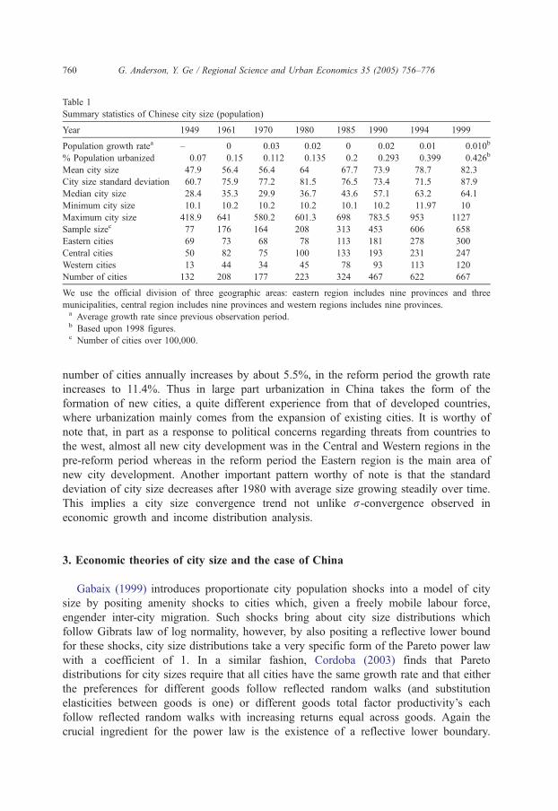
Table 1
Summary statistics of Chinese city size (population)
Year 1949 1961 1970 1980 1985 1990 1994 1999
Population growth ratea – 0 0.03 0.02 0 0.02 0.01 0.010b
% Population urbanized 0.07 0.15 0.112 0.135 0.2 0.293 0.399 0.426b
Mean city size 47.9 56.4 56.4 64 67.7 73.9 78.7 82.3
City size standard deviation 60.7 75.9 77.2 81.5 76.5 73.4 71.5 87.9
Median city size 28.4 35.3 29.9 36.7 43.6 57.1 63.2 64.1
Minimum city size 10.1 10.2 10.2 10.2 10.1 10.2 11.97 10
Maximum city size 418.9 641 580.2 601.3 698 783.5 953 1127
Sample sizec 77 176 164 208 313 453 606 658
Eastern cities 69 73 68 78 113 181 278 300
Central cities 50 82 75 100 133 193 231 247
Western cities 13 44 34 45 78 93 113 120
Number of cities 132 208 177 223 324 467 622 667
We use the official division of three geographic areas: eastern region includes nine provinces and three
municipalities, central region includes nine provinces and western regions includes nine provinces.a Average growth rate since previous observation period.b Based upon 1998 figures.c Number of cities over 100,000.
G. Anderson, Y. Ge / Regional Science and Urban Economics 35 (2005) 756–776760
number of cities annually increases by about 5.5%, in the reform period the growth rate
increases to 11.4%. Thus in large part urbanization in China takes the form of the
formation of new cities, a quite different experience from that of developed countries,
where urbanization mainly comes from the expansion of existing cities. It is worthy of
note that, in part as a response to political concerns regarding threats from countries to
the west, almost all new city development was in the Central and Western regions in the
pre-reform period whereas in the reform period the Eastern region is the main area of
new city development. Another important pattern worthy of note is that the standard
deviation of city size decreases after 1980 with average size growing steadily over time.
This implies a city size convergence trend not unlike r-convergence observed in
economic growth and income distribution analysis.
3. Economic theories of city size and the case of China
Gabaix (1999) introduces proportionate city population shocks into a model of city
size by positing amenity shocks to cities which, given a freely mobile labour force,
engender inter-city migration. Such shocks bring about city size distributions which
follow Gibrats law of log normality, however, by also positing a reflective lower bound
for these shocks, city size distributions take a very specific form of the Pareto power law
with a coefficient of 1. In a similar fashion, Cordoba (2003) finds that Pareto
distributions for city sizes require that all cities have the same growth rate and that either
the preferences for different goods follow reflected random walks (and substitution
elasticities between goods is one) or different goods total factor productivity’s each
follow reflected random walks with increasing returns equal across goods. Again the
crucial ingredient for the power law is the existence of a reflective lower boundary.
G. Anderson, Y. Ge / Regional Science and Urban Economics 35 (2005) 756–776 761
Duranton (2002) embeds a quality ladder model of growth in an urban framework, cities
grow or decline as they win or lose industries following new innovations so that small
technology shocks are the main engine of growth. Since there is no reflective lower
boundary in this model, it does not produce Zipf’s law (Pareto distributions for city
sizes) but, as the author notes, it does produce simulations that are well approximated by
a log normal distribution. Rossi-Hansberg and Wright (2004) propose a model in which
urban structure delivers a balance in the tension between the increasing returns to scale
gained from conurbations and the constant returns to scale required in the aggregate by
balanced growth. Shocks in this environment are finite order, finite moment industry
specific Markov shocks to productivity. Under some strong assumptions (either that
there is no physical capital or production is linear in physical capital with no human
capital) and by imposing a lower bound on the normalized process of city growth, it
produces Zipf’s law exactly. More generally, it produces deviations from Zipf’s law in
which small and large cities are under-represented, in essence the process displays a
reversion to mean property. An interesting feature of the model in the present context is
that the condition guaranteeing a constant number of cities over time is that human
capital growth exceeds population growth.
The introduction of independent proportionate shocks into a model is effectively an
application of bla loi de l’effet proportionnelQ employed in other contexts by Gibrat (1930,
1931). Gibrat’s law applied to city sizes is based on the premise that the initial city size
variate P0 is subject to a sequence of mutually independent proportionate changes vi, i=1,
2,. . ., t so that after the passage of time t, Pt=P0(1+v1)(1+v2): : : (1+vt). Assuming |vi| is
small relative to 1 and letting ln(1+vk)=l+lk where lk is an i.i.d. process with zero mean
and variance r2 which is small relative to 1 then:
lnPt ¼ l þ lnPt�1 þ ut ð1Þ
with l (again small relative to one) corresponding to the incremental drift or growth in city
size and ut corresponding to the increment of a drifting Weiner process which, after
sufficient passage of time t, renders the distribution of lnP as N(lnP0+(l�r/2)t,r2t). In
this framework the progress of city size is a random walk with drift, there is no long-run
bequilibriumQ city size that is the consequence of economic and physical forces, rather the
theory tells us about how the process is incrementing and that the variance of city sizes
will increase over time. Subsequently, by sacrificing the initial size independence
assumption, Kalecki (1945) modified Gibrat’s contribution to admit log normality with a
non-increasing variance. He proposed an alternative process which, in the present context,
replaces Eq. (1) with:
lnPt ¼ g þ lkt þ 1� kð ÞlnPt�1 þ ut ð2Þ
where 1NkN0. Kalecki establishes that, after a sufficient passage of time, the distribution of
lnP will be N((g+lkt)/k,r2/k2). Again l may be construed as the incremental growth
component but in this case the logarithm of the proportionate change in P is negatively
related to lnP via �k, note also the variance of the process is constant. Unlike Gibrat’s
model, economic forces are at work here determining equilibrium city size, albeit in a
simplistic fashion, since Eq. (2) may be re-written as a partial adjustment model with
(g+lt)/k as the target or equilibrium city size and k as the adjustment rate. In case (1) city

G. Anderson, Y. Ge / Regional Science and Urban Economics 35 (2005) 756–776762
size distributions are divergent through time and in case (2) city size distribution may be
thought of as convergent or at least non-divergent in the sense that whilst both models
predict increasing means Eq. (1) predicts increasing dispersion whereas Eq. (2) does not.
The distinction between the two is important because the former predicts a distribution that
advances in an unbounded fashion whereas the latter predicts a distribution whose location
trends through time with the growth rate but whose variance is bounded.
Obviously neither the Gibrat nor Kalecki models are consistent with the Pareto
distribution.4 Gabaix (1999), and also Cordoba (2003) and Rossi-Hansberg and Wright
(2004), establish the link by positing that the Geometric Brownian Motion describing city
size processes is subject to a reflective lower bound. Gabaix demonstrates that, provided
the growth rate of the number of cities does not exceed the growth rate of their
populations, the rank size distribution with a coefficient of one emerges as a consequence.
The introduction of a lower reflective boundary to processes such as Eqs. (1) and (2) so
that the logarithm of city size is not permitted to fall below some fixed lower bound lnpmin
causes the city size distribution to take the power form of a Pareto distribution with a
probability density f( p,pmin)=hpminhp�(1+h). Without the lower bound, city size would
follow Gibrat’s law of proportionate effects.
Reed (2001, 2002) proposes a closely related model with the same unbounded
Brownian motion but, under an assumption that cities have existed for a period T where T
is governed by an exponential distribution, develops a double Pareto distribution for city
size. This distribution yields a rank order rule for both upper and lower tails of the
distribution, respectively, of the form:
y*i ¼ ln Rank pið Þ=nð Þ ¼ lnb
a þ b
� �� aln
pi
p*
!þ ei for pi z p*
y*i ¼ ln Rank pið Þ=nð Þ ¼ lna
a þ b
� �� bln
pi
p*
!þ ei for pibp
* ð3Þ
Maximum likelihood estimates for a, b and p* are readily obtained from Eq. (3). In this
case city size follows a power law in both tails. Again for fixed T, city size would follow
Gibrat’s law.
Adapting these models to model the progress of Chinese city size distributions is
difficult. From the onset of the Republic to the introduction of Reforms in 1978, China
was very much a closed command economy where labor was not free to flow between
cities or between urban and rural sites and few of the assumptions required for the models
prevailed. During this time there were no constraints on fertility (indeed population growth
was positively encouraged during the earliest part of the Cultural Revolution) but there
was a bReturn to the LandQ policy wherein substantial portions of the urban population
were removed to rural areas and the authorities had a very deliberate policy of developing
4 Early models by Steindl (1965) and Simon (1955), based on assumptions regarding the relationship between
the rate at which cities emerged and the rate at which they grew, ran into difficulties because their preconditions
are basically counterfactual. Brakman et al. (1999) by introducing suitably calibrated negative externalities into a
general equilibrium location model are able to simulate rank size distributions.
G. Anderson, Y. Ge / Regional Science and Urban Economics 35 (2005) 756–776 763
cities in the interior for political reasons. Cities were not competing for new technologies
and were probably being sustained in their absence, the lack of freely flowing human
capital meant that amenity cost disparities could not be responded to. City sizes were still
subject to independent proportional shocks due to the vagaries of climate, population
growth, etc. but it is hard to rationalize policy making in the context of an economic model
during this period. With the reforms beginning in 1978, China opened up to trade,
loosened the restrictions on intercity migration, and abandoned the policy of deliberate city
development in the interior, almost coincidentally it also introduced the bOne Child
Family PolicyQ. The introduction of the reforms and the fertility policy in some sense took
the form of a large scale bnatural experimentQ so that a structural break in the progress of
city sizes is to be expected around the late 1970s.
With regard to the economic reforms there was a new found spirit of competition
for foreign markets so that some of the preconditions for the above cited city size
models began to prevail. However those theories do need to be augmented in order to
explain the inordinate growth in new cities during the reform period so that some
notion of the propensity for city births needs to be added. It is reasonable to assume
that a considerable disparity between urban and rural labor productivity had been
engendered by the restrictions imposed in the pre-reform period, so that considerable
gains were to be made by rapid urbanization. These could be realized one of two
ways, either by augmenting existing city populations or by initiating new cities. A
putty-clay technology for cities (Ottaviano and Thisse, 2001) would militate against
augmenting existing city populations, since diminishing productivity returns had
already set in and short-run congestion and amenity costs would increase considerably
at the margin. As for initiating new cities, the geographic advantages of the Eastern
Coastal region with its proximity to the newly liberated international trading routes,
probably offer greater net productivity gains and precipitated more rapid new city
development than in other regions. Thus while some reliance can be placed on the
above mentioned economic models of city size, it is probably appropriate to view this
period as one of adjustment from what was a position of extreme disequilibrium at the
onset of the period and it is probably the case that it is an adjustment process that has
not yet fully played itself out.
The introduction of an effective bOne Child per Family PolicyQ in the late 1970s
changed fundamentally the nature of population growth, especially in the cities where the
policy was most effectively monitored. Essentially the proportionate shocks to the model
(the ln(1+vt) implicit in Eqs. (1) and (2)) have themselves suffered a structural change in
the birth component of the shock. Simple statistical birth models (see, for example,
Whittle, 1970, p. 144) based upon a population size n at time t=0 with fertility intensity npredict, after time lapse t, a negative binomial population distribution with a mean and
variance of nent and nent(ent�1), respectively. The important point for present
considerations being that a reduction in fertility lowers not only the population growth
rate but also the population variance, thus the predictions of Gibrat’s law and Kalecki’s
modification also need to be qualified. In the case of the Gibrat model a reduction in the
variance of the shock process by d would attenuate the growth rate in the variance of city
sizes by r whereas in the Kalecki formulation it would bring about a systematic reduction
in the city size variance over time t of the form dP
i¼0 1� kð Þ2i, 0ViVt.

G. Anderson, Y. Ge / Regional Science and Urban Economics 35 (2005) 756–776764
4. Empirical results
4.1. The evolution of the city size distribution
The evolution of city size distributions depends upon two separate processes: the
expansion or shrinkage of existing cities and the city birth process. Most studies of
developed countries focus on the growth of existing cities because of the extremely low
birth rates of new cities. In the rapid urbanization process of China, new cities play an
important role in shaping the city size distribution. To explore the growth pattern of
existing cities, a balanced panel data set excluding all new cities formed and all cities that
deceased between 1961 and 1999 is constructed.5 A parallel study of both the balanced
and complete sample is employed.
First, the conventional rank size regression is employed to examine the evolution of the
Pareto exponent over time. Year 1980, the first observation in the reform years, is chosen
to be the benchmark. Time dummies and interaction terms are included to capture the
different intercepts and slopes in each year from 1980. The result is reported in Table 2.
Columns 2 and 4 of Table 2 report the estimated coefficients for the complete sample.
As may be observed, in 1980 there is a significant structural break in the evolution of
the Pareto exponent h. For the pre-reform period, 1949–1980, the estimated h is not
statistically significantly different from �1 at the 1% level. From 1980 to 1999, the size
distribution of the cities is increasingly convergent except for a slight reversal from 1994
to 1999. The Pareto exponents are significantly higher than 1 in the reform period,
which implies that the distribution of city size has become more equal than Zipf’s law
would predict. The intercepts are subject to more variation since they are directly
dependent on the sample sizes in each year. This pattern is different from the parallel
growth pattern of developed countries (Eaton and Eckstein, 1997; Dobkins and
Ioannides, 2000). The results for 149 existing cities, which are reported in columns 6
and 8, support a significant convergence trend in both pre-reform and reform period.
Simple plots of rank size functions reveal these patterns. Fig. 1(A) shows the shift of
rank size function over time for 149 existing cities. The rank size curves have become
flatter implying a consistent convergence trend over time. Fig. 1(B) shows the pattern
for the complete sample. The rank size curves in 1949 and 1980 have similar shape,
while the curve in 1999 becomes significantly flatter.
Non-parametric kernel density estimates of the relative city size distribution illustrate
the patterns indicated in the foregoing parametric analysis; Fig. 2 shows the relative size
distributions in 1949, 1980 and 1999. The main finding is consistent with the patterns
revealed in previous parametric analysis. The distributions in 1949 and 1980 are quite
similar, while the central mass significantly increased in the 1999 distribution. Quah
(1993) introduced Markov chain methods to analyze the transition between these relative
size distributions, here Dobkins and Ioannides (2000) is followed in assuming the size
distribution of existing cities follows a first-order homogeneous Markov process. Panels
A and B of Table 3 report the average decade transition matrix in the pre-reform and
5 This data set includes 149 cities and only covers the period from 1961 to 1999 because the paucity of
observations in 1949 render the balanced panel data set too small.

Table 2
Rank size regression, China 1949–1999
Complete sample Balanced panel
lnA 8.40T (0.11) lnp �1.08T (0.03) lnA 8.59T (0.10) lnp �1.15T (0.02)
D1949 �1.35T (0.20) D1949*lnp 0.02 (0.06)
D1961 �0.29T (0.16) D1961*lnp 0.003 (0.04) D1961 �0.64T (0.13) D1961*lnp (0.08)T (0.03)
D1970 �0.53T (0.16) D1970*lnp 0.03 (0.04) D1970 �0.70T (�0.13) D1970*lnp 0.09T (0.03)
D1985 0.85T (0.15) D1985*lnp �0.08T (0.04) D1985 0.32T (0.14) D1985*lnp �0.03 (0.03)
D1990 1.88T (0.14) D1990*lnp �0.19T (0.04) D1990 0.68T (0.15) D1990*lnp �0.07T (0.03)
D1994 2.68T (0.14) D1994*lnp �0.29T (0.04) D1994 0.95T (0.15) D1994*lnp �0.10T (0.04)
D1999 2.43T(0.14) D1999*lnp �0.22T (0.03) D1999 0.97T (0.15) D1999*lnp �0.07T (0.03)
Observations 2651 1043
Adjusted R-square 0.9 0.94
The dependent variable is log(rank of city size), lnA is the constant, Dt is the year dummies, lnp is log(city size).
Standard error in parentheses.
T Significant at 5%.
G. Anderson, Y. Ge / Regional Science and Urban Economics 35 (2005) 756–776 765
reform periods, respectively. The chosen intervals were based on 1/4, 1/2, 3/4, 1 and 2
times the sample mean.
Two features stand out. First, the diagonal entries indicate that larger cities have higher
persistence and smaller cities are more likely to move to upper categories. The trend of
upward concentration is more significant in the pre-reform period than in the reform period
which could be due to new entries in the lower tail. To examine this, the balanced panel of
149 cities existing from 1961 to 1999 is employed to calculate the distribution abstracted
from new entries and exits. The results, not reported here,6 indicate that a significant
concentration toward the upper tail of the distribution remains, suggesting real growth in
city size as well as new entrants is causing the phenomenon (a pattern quite different from
that of France and Japan (Eaton and Eckstein, 1997)).
A second feature is apparent in the last row of the table which shows the frequency
distribution of new entrants. The relative size of new cities is significantly different
before and after 1980. In the pre-reform period, 77% of new cities are smaller than half
of the mean. In the reform period, 79% of new cities are medium size (from half the
mean to twice the mean). Recalling that the observation interval in the reform period is
10 years or shorter this is truly remarkable. It implies that settlements too small to be
classified as cities in the distribution at the onset of the interval between observation
periods have grown to such a size as to merit their entrance in the middle of the
distribution within 10 years.
Combinations of the growth processes of existing cities and the pattern of new entrants
explain the difference in city size evolution in pre-reform and post-reform periods. In the
pre-reform period, the new entrants concentrate in the lower tail and raise the relative size
ranking of existing cities. For existing cities, small cities expand into the middle range
with the big cities in the upper tail exhibiting strong downward immobility. The
combination of these two movements results in a relatively stable size distribution which is
6 Available from the authors on request.

2
02
46
3 4 5 6 7Inpop1949/Inpop1980/Inpop1999
B
Inra
nk19
49/In
rank
1980
/Inra
nk19
99
Inrank1949Inrank1999
Inrank1980
2
02
31
45
3 4 5 6 7Inpop1961/Inpop1980/Inpop1999
A
Inra
nk19
61/In
rank
1980
/Inra
nk19
99
Inrank1961Inrank1999
Inrank1980
Fig. 1. (A) Rank size plots for 149 cities in balanced panel sample in 1961, 1980 and 1999. (B) Rank size plots for
complete sample in 1949, 1980 and 1999.
G. Anderson, Y. Ge / Regional Science and Urban Economics 35 (2005) 756–776766
not significantly different from the prediction of Zipf’s law. In the reform period, the
existing small cities grow faster than larger cities and new entrants concentrate around the
middle size. As a result, the size distribution exhibits a strong convergence trend.

Fig. 2. Kernel estimate of log relative city size distribution, 1949, 1980 and 1999. Note 1: kernel estimates were
based upon the Epanechnikov kernel. Note 2: relative city size is defined as the city population divided by the
sample mean in each year.
G. Anderson, Y. Ge / Regional Science and Urban Economics 35 (2005) 756–776 767
4.2. Statistical tests of alternative distributions
It has been common in empirical work in this field to interpret results of rank size
regressions reported in Table 2 as evidence favoring the Pareto distribution and in
particular as support for Zipf’s law. However they do not constitute tests of the assumption
that the data are generated by a Pareto distribution. Furthermore they only constitute an
Table 3
Upper boundary 0.25 0.5 0.75 1 2 l Exits
Panel A: Average decade transition matrix in pre-reform period (1949–1980)
0.25 0.3 0.35 0.19 0.04 0 0 0.12
0.5 0.03 0.47 0.27 0.06 0.1 0 0.07
0.75 0.02 0.03 0.46 0.26 0.18 0.02 0.03
1 0 0.05 0.06 0.29 0.46 0.07 0.07
2 0 0.04 0.03 0.03 0.64 0.14 0.12
l 0 0 0.02 0 0.02 0.96 0
Entrants 0.44 0.33 0.07 0.06 0.09 0.01
Panel B: Average decade transition matrix in reform period (1980–1999)
0.25 0.58 0.25 0.09 0 0.05 0 0.03
0.5 0.02 0.65 0.17 0.04 0.08 0.02 0.02
0.75 0 0.03 0.77 0.13 0.06 0 0.01
1 0 0.05 0.07 0.75 0.11 0 0.02
2 0 0.04 0.03 0.05 0.82 0.04 0.01
l 0 0 0 0 0.04 0.96 0
Entry 0.08 0.13 0.25 0.2 0.34 0.01

Table 4
Test of alternative distributions (complete samples of cities, 1949–1999)
Year Sample size Log normal distributionf Pareto distributione,f Double Pareto distributione,f
v2(7)a [18.46] lb rc v2(8)a [20.09] hML hOLS v2(6)a [15.09] aML bML pML*
1949 77 7.8 3.46 0.83 12.48 0.87 0.914 –d 0.88 – 3.46
1961 176 8.89 3.61 0.84 36.84 0.78 0.859 –d 0.78 – 3.61
1970 164 16 3.57 0.88 21 0.8 0.875 –d 0.81 – 3.57
1980 208 20.85 3.73 0.85 60.75 0.71 0.799 785.6 1.47 1.74 3.73
1985 313 11.31 3.87 0.78 187.93 0.64 0.737 1109.6 1.6 1.81 3.87
1990 435 17.62 4.03 0.7 446.89 0.58 0.679 1590.1 1.79 1.77 4.03
1994 606 5.02 4.14 0.65 686.57 0.6 0.702 2117.7 1.98 1.94 4.14
1999 658 11.39 4.16 0.66 822.21 0.54 0.626 2266.6 1.98 2 4.16
a v(K) is a goodness-of-fit test (with K degrees of freedom) of the null hypothesis that the distributional
specification is appropriate. The number in the square bracket corresponds to the 1% critical value.b Sample mean.c Sample standard deviation.d For the first three observation years the information matrix was singular with the estimates converging to the
single Pareto distribution.e Subscripts ML and OLS refer respectively to the maximum likelihood and ordinary least squares estimates.f In all goodness-of-fit and divergence tests reported here partitions were chosen to generate 10 equiprobable
cells or regions.
G. Anderson, Y. Ge / Regional Science and Urban Economics 35 (2005) 756–776768
indirect test of Zipf’s law in that, whilst the regression coefficient may not be significantly
different from one, the underlying distribution may not be Pareto. As a consequence,
efficient OLS estimates together with maximum likelihood estimates of the Pareto
coefficients together with the corresponding goodness-of-fit tests (Pearson, 1900) are
reported in Table 4. In addition the table reports maximum likelihood estimates of the log
normal and double Pareto models together with the corresponding goodness-of-fit tests.
The first thing to note is that the maximum likelihood estimates and the restricted
regression estimates for the Pareto coefficient are consistently lower than the standard OLS
estimates in Table 2 and uniformly lower than 1 in absolute value. The Zipf’s restriction
(h=1) is rejected in every instance except 1949. In addition the goodness-of-fit tests
strongly reject the Pareto Distribution hypothesis in all but the 1949 observation set. With
respect to the double Pareto estimates in the first three observation years the information
matrix is singular with the estimates converging to a single rather than double Pareto
specification. Apart from estimates of p* (which are closely related to the sample means),
parameter estimates change little from period to period relative to their standard deviation
in the remaining years, again the goodness-of-fit tests strongly reject the double Pareto
hypothesis. With regard to the Gibrat and Kalecki log normality specifications, the
goodness-of-fit tests, with one exception (1980) fail to reject the null hypothesis of log
normality at the 1% level, suggesting that the log normal model is a much better
rationalization of the data.7 The mean of the distribution indicates annualized percentage
7 This is in striking contrast to results for the USA (obtainable from the authors upon request) where although the
Zipf restriction is rejected in 3 of 6 cases the Pareto distribution is never rejected at the 1% level and the coefficient
estimates are uniformly higher than 1 in absolute value. On the other hand log-normality is strongly rejected in every
case. Note that under a more general (urban place) definition of cities which essentially rules out the lower boundary
for city size Eeckhout (in press) finds the log normal distribution to be the preferred specification.

G. Anderson, Y. Ge / Regional Science and Urban Economics 35 (2005) 756–776 769
city size growth rates between successive observation periods of 0.73, �0.78, 1.84, 4.08,
4.34, 3.57 and 0.30 assuming a Gibrat process and 1.24, �0.45, 1.64, 2.87, 3.02, 2.66 and
0.47 assuming a Kalecki process. One aspect is perplexing for advocates of the Gibrat
model, namely the diminishing estimates of the standard deviation over time from 1970
onwards. Under the Geometric Brownian Motion assumption the sample standard
deviation is an estimate of rMT and should be increasing with the passing of time.
The unprecedented urbanization rates in China, especially during the reform period,
meant that in some sample years new cities represent an increase of 50% in the sample.
Table 5 reports the results corresponding to Table 4 when the sample is restricted to cities
that have remained in the sample from 1961 to 1999, a panel of existing cities as it were.
The results are unaltered in substance, Pareto and double Pareto specifications are strongly
rejected by the data whereas log normality appears to accord with the data extremely well
throughout the period. City size growth rates are of a similar magnitude to the full sample,
though the average city size is larger, consistent with them being the longer lived cities.
The phenomenon of the diminishing standard deviation of city sizes after the 1970s is also
still conspicuous though not as strong.
The full sample results are illustrated in Figs. 3–6 for 1949, 1980, 1990 and 1999,
respectively, which overlay kernel estimates of the empirical probability distribution
function on respective plots of the estimated Pareto, double Pareto and log normal
distribution functions. Perusal of the diagrams makes it quite clear how it is that the log
normal formulation best fits the data. Kernel estimates of the distributions always generate
modal points above the minimum city size (unlike the Pareto distribution) and the modal
points always appear to be points of continuity (unlike the double Pareto distribution). The
close proximity of the log normal distribution to the kernel density estimate (relative to the
other distributions) in each case attests to it providing the best fit. The issue remains as to
whether convergence or divergence underlays the data generating process for China.
The standard F-test for variance ratios is notoriously bad when the underlaying data
generating processes diverge from normality (Anderson, 2001), furthermore divergence or
polarization need not result in increased variances (Wolfson, 1994). The problem may be
resolved by resorting to modifications of a test analogous to the goodness-of-fit test
(herein denoted PAT for Pearson Analogue Test) used to examine the similarity between
two samples (Anderson, 2001, 2004). Letting OkA be the observed proportion of
Table 5
Test of alternative distributions (balanced panel, 1961–1999)
Year Sample
size
Log normal distribution Pareto distribution Double Pareto distribution
v2(7)a
[18.46]
lb rc v2(8)a
[20.09]
hML hOLS v2(6)a
[15.09]
aML bML pML*
1961 149 7.3 3.7 0.85 414.2 0.233 0.259 567.74 1.4 1.35 3.58
1970 149 9.41 3.7 0.86 393.91 0.231 0.257 570.62 1.4 1.48 3.54
1980 149 12.64 4 0.8 426.31 0.23 0.254 570.87 1.5 1.76 3.82
1985 149 12.79 4.2 0.77 462.79 0.221 0.243 557.67 1.6 1.75 4.02
1990 149 11.38 4.3 0.75 433.35 0.222 0.243 549.24 1.6 1.8 4.19
1994 149 11.52 4.4 0.73 453.77 0.226 0.247 556.66 1.7 1.92 4.3
1999 149 15.18 4.6 0.76 478.56 0.213 0.233 556.79 1.6 1.89 4.43
See Table 4.
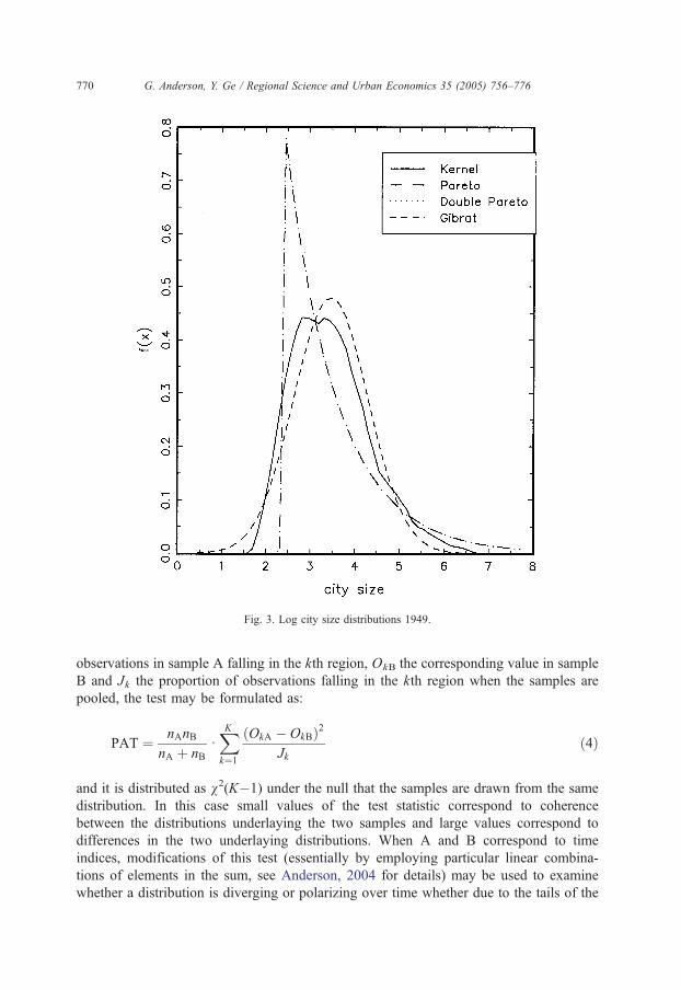
Fig. 3. Log city size distributions 1949.
G. Anderson, Y. Ge / Regional Science and Urban Economics 35 (2005) 756–776770
observations in sample A falling in the kth region, OkB the corresponding value in sample
B and Jk the proportion of observations falling in the kth region when the samples are
pooled, the test may be formulated as:
PAT ¼ nAnB
nA þ nBdXKk¼1
OkA � OkBð Þ2
Jkð4Þ
and it is distributed as v2(K�1) under the null that the samples are drawn from the same
distribution. In this case small values of the test statistic correspond to coherence
between the distributions underlaying the two samples and large values correspond to
differences in the two underlaying distributions. When A and B correspond to time
indices, modifications of this test (essentially by employing particular linear combina-
tions of elements in the sum, see Anderson, 2004 for details) may be used to examine
whether a distribution is diverging or polarizing over time whether due to the tails of the

Fig. 4. Log city size distributions 1980.
G. Anderson, Y. Ge / Regional Science and Urban Economics 35 (2005) 756–776 771
distribution moving apart or to there being increased concentration in them. To establish
divergence when progressing from A to B the test has to be used twice, once to bnotrejectQ divergence in moving from A to B and once to reject divergence from B to A.
The results are reported in Table 6.
Assuming divergence in distribution to be reflected in increased variances a simple F-
test is appropriate, column 2 of Table 6 reports this. As may be observed the test is unable
to detect any discernable change in variance from period to period except for 1985 to 1990
and 1990 to 1994 when variance reductions were indicated at the 5% level. As noted
earlier this test has notoriously bad size and power properties and divergence need not
imply variance change. Columns 3 through 6 of Table 6 report the details of divergence
tests of the first and second order which, when considered at the 5% critical level, indicate
no divergence or convergence from 1949 through to 1980 and convergence of both types
(tails getting closer together and appearing less concentrated) from 1980 through to 1994
with divergence occurring from 1994 to 1999. It may be concluded that convergence

Fig. 5. Log city size distributions 1990.
G. Anderson, Y. Ge / Regional Science and Urban Economics 35 (2005) 756–776772
appears to be the predominant force in the economic reform period suggesting that the
Kalecki formulation rather than Gibrats formulation underlays the city size data generating
process. Thus Chinese cities may be thought of as converging to an equilibrium city size
which is itself trending upward through time.
5. Conclusions
Whilst data on Chinese city sizes yield results for commonly employed rank size
regressions that accord with the conventional wisdom of a Pareto distribution, closer
examination reveals the Chinese case to be substantially different with evidence strongly
favoring a log normal distribution. The two distributions are linked. Describing the
progress of city sizes through time by a Geometric Brownian Motion engenders a log
normal city size distribution at a given point in time. Gabaix (1999) demonstrates that,
when the Geometric Brownian Motion is constrained by a lower reflective boundary, a
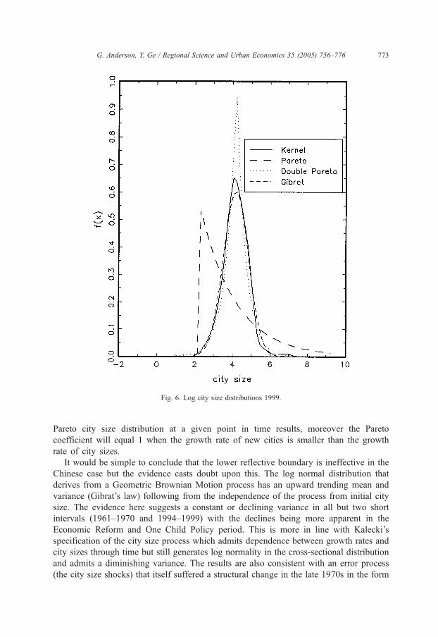
Fig. 6. Log city size distributions 1999.
G. Anderson, Y. Ge / Regional Science and Urban Economics 35 (2005) 756–776 773
Pareto city size distribution at a given point in time results, moreover the Pareto
coefficient will equal 1 when the growth rate of new cities is smaller than the growth
rate of city sizes.
It would be simple to conclude that the lower reflective boundary is ineffective in the
Chinese case but the evidence casts doubt upon this. The log normal distribution that
derives from a Geometric Brownian Motion process has an upward trending mean and
variance (Gibrat’s law) following from the independence of the process from initial city
size. The evidence here suggests a constant or declining variance in all but two short
intervals (1961–1970 and 1994–1999) with the declines being more apparent in the
Economic Reform and One Child Policy period. This is more in line with Kalecki’s
specification of the city size process which admits dependence between growth rates and
city sizes through time but still generates log normality in the cross-sectional distribution
and admits a diminishing variance. The results are also consistent with an error process
(the city size shocks) that itself suffered a structural change in the late 1970s in the form
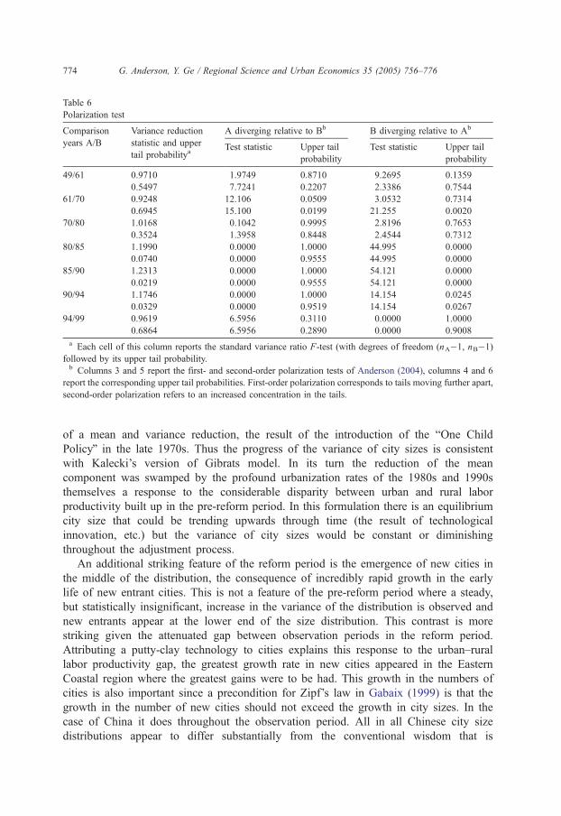
Table 6
Polarization test
Comparison
years A/B
Variance reduction
statistic and upper
tail probabilitya
A diverging relative to Bb B diverging relative to Ab
Test statistic Upper tail
probability
Test statistic Upper tail
probability
49/61 0.9710 1.9749 0.8710 9.2695 0.1359
0.5497 7.7241 0.2207 2.3386 0.7544
61/70 0.9248 12.106 0.0509 3.0532 0.7314
0.6945 15.100 0.0199 21.255 0.0020
70/80 1.0168 0.1042 0.9995 2.8196 0.7653
0.3524 1.3958 0.8448 2.4544 0.7312
80/85 1.1990 0.0000 1.0000 44.995 0.0000
0.0740 0.0000 0.9555 44.995 0.0000
85/90 1.2313 0.0000 1.0000 54.121 0.0000
0.0219 0.0000 0.9555 54.121 0.0000
90/94 1.1746 0.0000 1.0000 14.154 0.0245
0.0329 0.0000 0.9519 14.154 0.0267
94/99 0.9619 6.5956 0.3110 0.0000 1.0000
0.6864 6.5956 0.2890 0.0000 0.9008
a Each cell of this column reports the standard variance ratio F-test (with degrees of freedom (nA�1, nB�1)
followed by its upper tail probability.b Columns 3 and 5 report the first- and second-order polarization tests of Anderson (2004), columns 4 and 6
report the corresponding upper tail probabilities. First-order polarization corresponds to tails moving further apart,
second-order polarization refers to an increased concentration in the tails.
G. Anderson, Y. Ge / Regional Science and Urban Economics 35 (2005) 756–776774
of a mean and variance reduction, the result of the introduction of the bOne Child
PolicyQ in the late 1970s. Thus the progress of the variance of city sizes is consistent
with Kalecki’s version of Gibrats model. In its turn the reduction of the mean
component was swamped by the profound urbanization rates of the 1980s and 1990s
themselves a response to the considerable disparity between urban and rural labor
productivity built up in the pre-reform period. In this formulation there is an equilibrium
city size that could be trending upwards through time (the result of technological
innovation, etc.) but the variance of city sizes would be constant or diminishing
throughout the adjustment process.
An additional striking feature of the reform period is the emergence of new cities in
the middle of the distribution, the consequence of incredibly rapid growth in the early
life of new entrant cities. This is not a feature of the pre-reform period where a steady,
but statistically insignificant, increase in the variance of the distribution is observed and
new entrants appear at the lower end of the size distribution. This contrast is more
striking given the attenuated gap between observation periods in the reform period.
Attributing a putty-clay technology to cities explains this response to the urban–rural
labor productivity gap, the greatest growth rate in new cities appeared in the Eastern
Coastal region where the greatest gains were to be had. This growth in the numbers of
cities is also important since a precondition for Zipf’s law in Gabaix (1999) is that the
growth in the number of new cities should not exceed the growth in city sizes. In the
case of China it does throughout the observation period. All in all Chinese city size
distributions appear to differ substantially from the conventional wisdom that is

G. Anderson, Y. Ge / Regional Science and Urban Economics 35 (2005) 756–776 775
embodied in Zipf’s law and appear to have been affected in a predictable fashion by the
Economic Reform and One Child Per Family policies to the extent that a structural
change does appear to have occurred at the onset of the reform period.
Acknowledgments
The authors would like to thank the editor and two referees for their very helpful
comments on earlier versions of this paper. Thanks are also due to the SSHRC for support
under research grant number 410040254.
References
Anderson, G.J., 2001. The power and size of nonparametric tests for common distributional characteristics.
Econometric Reviews 20, 1–30.
Anderson, G.J., 2004. Toward an empirical analysis of polarization. Journal of Econometrics 122, 1–26.
Auerbach, F., 1913. Das Gesetz der Belvolkerungskoncertration. Petermanns Geographische Mitteilungen 59,
74–76.
Black, D., Henderson, V., 1999. A theory of urban growth. Journal of Political Economy 107, 252–284.
Brakman, S., Garretsen, H., Van Marrewijk, C., van den Berg, M., 1999. The return of Zipf: toward a further
understanding of the rank size distribution. Journal of Regional Science 39, 183–213.
Cordoba, J.-C., 2003. On the Distribution of City Sizes. Mimeo, Economics Department, Rice University.
Dobkins, L., Ioannides, Y., 2000. Dynamic evolution of the U.S. city size distribution. In: Huriot, J.M., Thisse,
J.F. (Eds.), Economics of Cities. Cambridge University Press, pp. 217–260.
Duranton, G., 2002. City size distributions as a consequence of the growth process. Mimeo, London, School of
Economics.
Eaton, J., Eckstein, Z., 1997. City and growth: theory and evidence from France and Japan. Regional Science
and Urban Economics 17, 443–474.
Eeckhout, J., in press. Gibrat’s law for (all) cities. American Economic Review.
Gabaix, X., 1999. Zipf’s law for cities: an explanation. Quarterly Journal of Economics 114, 739–767.
Gabaix, X., Ioannides, Y.M., 2004. The evolution of city size distributions. In: Vernon Henderson, J.,
Thisse, J.F., (Eds.), Handbook of Regional and Urban Economics, vol. 4. North Holland, Amsterdam,
pp. 2341–2378. Chapter 53.
Gibrat, R., 1930. Une Loi Des Repartitions Economiques: L’effet Proportionelle. Bulletin de Statistique General,
France 19, 469.
Gibrat, R., 1931. Les Inegalites Economiques (Libraire du Recueil Sirey Paris).
Ioannides, Y.M., Overman, H.G., 2003. Zipf’s law for cities: an empirical examination. Regional Science and
Urban Economics 33, 127–137.
Kalecki, M., 1945. On the Gibrat distribution. Econometrica 13, 161–170.
Ottaviano, G.I.P., Thisse, J.F., 2001. On economic geography in economic theory: increasing returns and
pecuniary externalities. Journal of Economic Geography 1, 153–179.
Overman, H.G., Ioannides, Y.M., 2001. Cross-sectional evolution of the U.S. city size distribution. Journal of
Urban Economics 49, 543–566.
Pareto, V., 1897. Cours d’Economie Politique (Rouge et Cie Paris).
Pearson, K., 1900. On a criterion that a given system of deviations from the probable in the case of a correlated
system of variables is such that it can reasonably be supposed to have arisen from random sampling.
Philosophical Magazine 50, 157–175.
Quah, D., 1993. Empirical cross-section dynamics in economic growth. European Economic Review 37,
426–434.
Reed, W.J., 2001. The Pareto, Zipf and other power laws. Economics Letters 74, 15–19.

G. Anderson, Y. Ge / Regional Science and Urban Economics 35 (2005) 756–776776
Reed, W.J., 2002. On the rank-size distribution for human settlements. Journal of Regional Science 41, 1–17.
Rosen, K.T., Resnick, M., 1980. The size distribution of cities: an examination of the Pareto law and primacy.
Journal of Urban Economics 8, 165–186.
Rossi-Hansberg, E., Wright, M., 2004. Urban structure and growth. Mimeo, Stanford University, Economics
Department.
Sharma, S., 2003. Persistence and stability in city growth. Journal of Urban Economics 53, 300–320.
Simon, H., 1955. On a class of skew distribution functions. Biometrica 42, 425–440.
Soo, K.T., in press. Zipf’s law for cities: a cross country investigation. Regional Science and Urban Economics.
State Statistical Bureau, 1990. Forty Years of Urban Development. China Statistic Press, Beijing.
State Statistical Bureau, 1991–2000. Chinese Urban Statistical Yearbooks. China Statistic Press, Beijing.
Steindl, J., 1965. Random Processes and the Growth of Firms. Hafner, New York.
Whittle, P., 1970. Probability. Wiley.
Wolfson, M.C., 1994. When inequalities diverge. Papers and Proceedings-American Economic Review 84,
353–358.
Zipf, G., 1949. Human Behavior and the Principle of Last Effort. Addison Wesley, Cambridge, MA.