Embed Size (px)
Citation preview

The Social Dynamics of Stigma:Supplemental Appendices
Myong-Hun Chang† and Joseph E. Harrington, Jr.‡
June 6, 2017
This Appendix consists of three parts:
Appendix A: Correlation between the Rate of Acceptance and the Rate of Disclosure
Appendix B: Parameterizations for Robustness Check
Appendix C: Source Code for the Benchmark Simulation
†Department of Economics, Cleveland State University, Cleveland, OH 44115; [email protected]
‡Patrick T. Harker Professor, Department of Business Economics & Public Policy, The Wharton School, University of Pennsylvania, PA 19104;
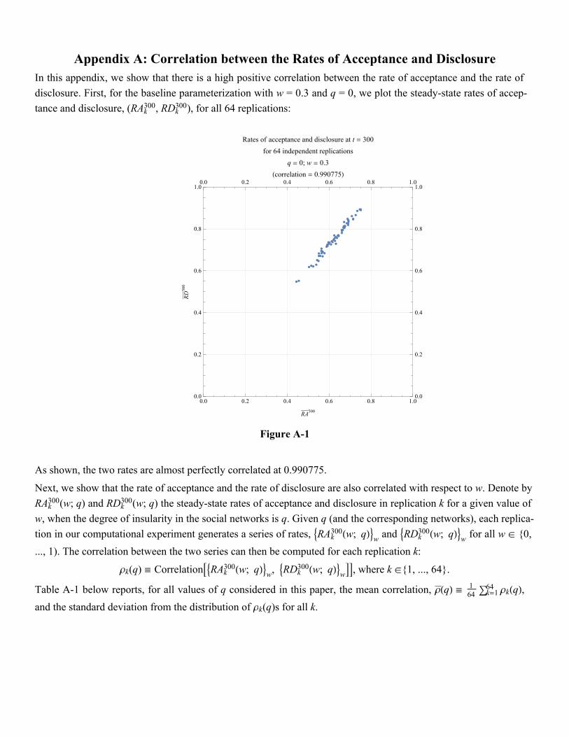
Appendix A: Correlation between the Rates of Acceptance and DisclosureIn this appendix, we show that there is a high positive correlation between the rate of acceptance and the rate of
disclosure. First, for the baseline parameterization with w = 0.3 and q = 0, we plot the steady-state rates of accep-
tance and disclosure, (RAk300, RDk
300), for all 64 replications:
0.0 0.2 0.4 0.6 0.8 1.00.0
0.2
0.4
0.6
0.8
1.00.0 0.2 0.4 0.6 0.8 1.0
0.0
0.2
0.4
0.6
0.8
1.0
RA300
RD
300
Rates of acceptance and disclosure at t = 300
for 64 independent replications
q = 0; w = 0.3
(correlation = 0.990775)
Figure A-1
As shown, the two rates are almost perfectly correlated at 0.990775.
Next, we show that the rate of acceptance and the rate of disclosure are also correlated with respect to w. Denote by
RAk300(w; q) and RDk
300(w; q) the steady-state rates of acceptance and disclosure in replication k for a given value of
w, when the degree of insularity in the social networks is q. Given q (and the corresponding networks), each replica-
tion in our computational experiment generates a series of rates, RAk300(w; q)
w and RDk
300(w; q)w
for all w ∈ {0,
..., 1). The correlation between the two series can then be computed for each replication k:
ρk(q) ≡ CorrelationRAk300(w; q)
w, RDk
300(w; q)w, where k ∈{1, ..., 64}.
Table A-1 below reports, for all values of q considered in this paper, the mean correlation, ρ(q) ≡ 164 ∑k=1
64 ρk(q),
and the standard deviation from the distribution of ρk(q)s for all k.
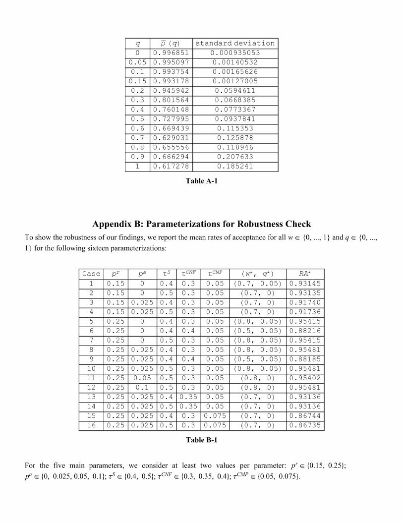
q ρ (q) standard deviation0 0.996851 0.000935053
0.05 0.995097 0.001405320.1 0.993754 0.001656260.15 0.993178 0.001270050.2 0.945942 0.05946110.3 0.801564 0.06683850.4 0.760148 0.07733670.5 0.727995 0.09378410.6 0.669439 0.1153530.7 0.629031 0.1258780.8 0.655556 0.1189460.9 0.666294 0.2076331 0.617278 0.185241
Table A-1
Appendix B: Parameterizations for Robustness CheckTo show the robustness of our findings, we report the mean rates of acceptance for all w ∈ {0, ..., 1} and q ∈ {0, ...,
1} for the following sixteen parameterizations:
Case pr pa τS τCNF τCMP (w*, q*) RA*
1 0.15 0 0.4 0.3 0.05 (0.7, 0.05) 0.931452 0.15 0 0.5 0.3 0.05 (0.7, 0) 0.931353 0.15 0.025 0.4 0.3 0.05 (0.7, 0) 0.917404 0.15 0.025 0.5 0.3 0.05 (0.7, 0) 0.917365 0.25 0 0.4 0.3 0.05 (0.8, 0.05) 0.954156 0.25 0 0.4 0.4 0.05 (0.5, 0.05) 0.882167 0.25 0 0.5 0.3 0.05 (0.8, 0.05) 0.954158 0.25 0.025 0.4 0.3 0.05 (0.8, 0.05) 0.954819 0.25 0.025 0.4 0.4 0.05 (0.5, 0.05) 0.8818510 0.25 0.025 0.5 0.3 0.05 (0.8, 0.05) 0.9548111 0.25 0.05 0.5 0.3 0.05 (0.8, 0) 0.9540212 0.25 0.1 0.5 0.3 0.05 (0.8, 0) 0.9548113 0.25 0.025 0.4 0.35 0.05 (0.7, 0) 0.9313614 0.25 0.025 0.5 0.35 0.05 (0.7, 0) 0.9313615 0.25 0.025 0.4 0.3 0.075 (0.7, 0) 0.8674416 0.25 0.025 0.5 0.3 0.075 (0.7, 0) 0.86735
Table B-1
For the five main parameters, we consider at least two values per parameter: pr ∈ {0.15, 0.25};
pa ∈ {0, 0.025, 0.05, 0.1}; τS ∈ {0.4, 0.5}; τCNF ∈ {0.3, 0.35, 0.4}; τCMP ∈ {0.05, 0.075}.

The second from the last column indicates the pair of values for w and q, (w*, q*), that maximizes the mean rate
of acceptance. The last column reports the corresponding rate of acceptance, RA*.
More detailed information is provided next for each of the sixteen parameterizations. Specifically, for each case we
present a numerical table reporting the mean rate of acceptance for all values of w and q at the top. Below each
table, we provide three figures that visualize the results in the table: a) 3-D surface plot; b) the contour plot; and c)
the multiple line plot for each value of q.
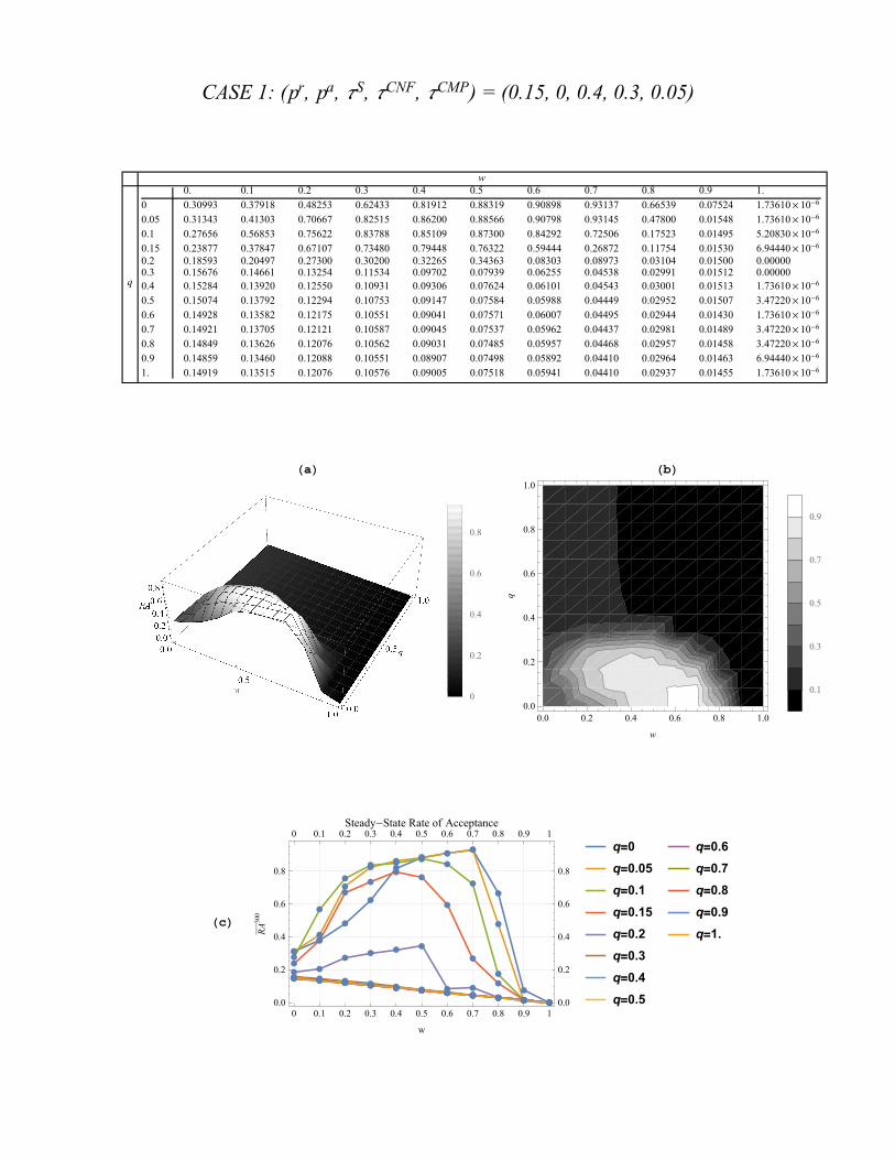
CASE 1: (pr, pa, τS, τCNF, τCMP) = (0.15, 0, 0.4, 0.3, 0.05)
w
q
0. 0.1 0.2 0.3 0.4 0.5 0.6 0.7 0.8 0.9 1.
0 0.30993 0.37918 0.48253 0.62433 0.81912 0.88319 0.90898 0.93137 0.66539 0.07524 1.73610×10⁻⁶
0.05 0.31343 0.41303 0.70667 0.82515 0.86200 0.88566 0.90798 0.93145 0.47800 0.01548 1.73610×10⁻⁶
0.1 0.27656 0.56853 0.75622 0.83788 0.85109 0.87300 0.84292 0.72506 0.17523 0.01495 5.20830×10⁻⁶
0.15 0.23877 0.37847 0.67107 0.73480 0.79448 0.76322 0.59444 0.26872 0.11754 0.01530 6.94440×10⁻⁶
0.2 0.18593 0.20497 0.27300 0.30200 0.32265 0.34363 0.08303 0.08973 0.03104 0.01500 0.000000.3 0.15676 0.14661 0.13254 0.11534 0.09702 0.07939 0.06255 0.04538 0.02991 0.01512 0.000000.4 0.15284 0.13920 0.12550 0.10931 0.09306 0.07624 0.06101 0.04543 0.03001 0.01513 1.73610×10⁻⁶
0.5 0.15074 0.13792 0.12294 0.10753 0.09147 0.07584 0.05988 0.04449 0.02952 0.01507 3.47220×10⁻⁶
0.6 0.14928 0.13582 0.12175 0.10551 0.09041 0.07571 0.06007 0.04495 0.02944 0.01430 1.73610×10⁻⁶
0.7 0.14921 0.13705 0.12121 0.10587 0.09045 0.07537 0.05962 0.04437 0.02981 0.01489 3.47220×10⁻⁶
0.8 0.14849 0.13626 0.12076 0.10562 0.09031 0.07485 0.05957 0.04468 0.02957 0.01458 3.47220×10⁻⁶
0.9 0.14859 0.13460 0.12088 0.10551 0.08907 0.07498 0.05892 0.04410 0.02964 0.01463 6.94440×10⁻⁶
1. 0.14919 0.13515 0.12076 0.10576 0.09005 0.07518 0.05941 0.04410 0.02937 0.01455 1.73610×10⁻⁶
(a) (b)
0
0.2
0.4
0.6
0.8
0.0 0.2 0.4 0.6 0.8 1.00.0
0.2
0.4
0.6
0.8
1.0
w
q
0.1
0.3
0.5
0.7
0.9
(c)
0 0.1 0.2 0.3 0.4 0.5 0.6 0.7 0.8 0.9 10.0
0.2
0.4
0.6
0.8
0 0.1 0.2 0.3 0.4 0.5 0.6 0.7 0.8 0.9 1
0.0
0.2
0.4
0.6
0.8
w
RA
300
Steady-State Rate of Acceptance
q=0
q=0.05
q=0.1
q=0.15
q=0.2
q=0.3
q=0.4
q=0.5
q=0.6
q=0.7
q=0.8
q=0.9
q=1.

CASE 2: (pr, pa, τS, τCNF, τCMP) = (0.15, 0, 0.5, 0.3, 0.05)
w
q
0. 0.1 0.2 0.3 0.4 0.5 0.6 0.7 0.8 0.9 1.
0 0.18070 0.19535 0.21914 0.28309 0.44111 0.77811 0.90705 0.93135 0.63643 0.07524 1.73610×10⁻⁶
0.05 0.16622 0.16939 0.18318 0.22640 0.58245 0.87328 0.90785 0.89051 0.43500 0.01548 1.73610×10⁻⁶
0.1 0.15971 0.15600 0.15556 0.16372 0.26480 0.55597 0.67593 0.54863 0.14647 0.01495 5.20830×10⁻⁶
0.15 0.15405 0.14676 0.13979 0.13147 0.12413 0.15674 0.16883 0.11891 0.05977 0.01530 6.94440×10⁻⁶
0.2 0.15195 0.14405 0.13311 0.11983 0.10509 0.09028 0.06555 0.04799 0.03048 0.01500 0.000000.3 0.14880 0.13902 0.12731 0.11177 0.09551 0.07839 0.06214 0.04535 0.02990 0.01512 0.000000.4 0.14919 0.13653 0.12385 0.10848 0.09272 0.07612 0.06099 0.04543 0.03001 0.01513 1.73610×10⁻⁶
0.5 0.14870 0.13656 0.12221 0.10718 0.09127 0.07582 0.05987 0.04449 0.02952 0.01507 3.47220×10⁻⁶
0.6 0.14784 0.13500 0.12136 0.10535 0.09032 0.07568 0.06007 0.04495 0.02944 0.01430 1.73610×10⁻⁶
0.7 0.14801 0.13633 0.12082 0.10569 0.09038 0.07534 0.05962 0.04437 0.02981 0.01489 3.47220×10⁻⁶
0.8 0.14734 0.13559 0.12042 0.10549 0.09023 0.07482 0.05957 0.04468 0.02957 0.01458 3.47220×10⁻⁶
0.9 0.14749 0.13387 0.12051 0.10544 0.08899 0.07497 0.05891 0.04410 0.02964 0.01463 6.94440×10⁻⁶
1. 0.14805 0.13453 0.12059 0.10566 0.09001 0.07516 0.05941 0.04410 0.02937 0.01455 1.73610×10⁻⁶
(a) (b)
0
0.2
0.4
0.6
0.8
0.0 0.2 0.4 0.6 0.8 1.00.0
0.2
0.4
0.6
0.8
1.0
w
q
0.1
0.3
0.5
0.7
0.9
(c)
0 0.1 0.2 0.3 0.4 0.5 0.6 0.7 0.8 0.9 10.0
0.2
0.4
0.6
0.8
0 0.1 0.2 0.3 0.4 0.5 0.6 0.7 0.8 0.9 1
0.0
0.2
0.4
0.6
0.8
w
RA
300
Steady-State Rate of Acceptance
q=0
q=0.05
q=0.1
q=0.15
q=0.2
q=0.3
q=0.4
q=0.5
q=0.6
q=0.7
q=0.8
q=0.9
q=1.
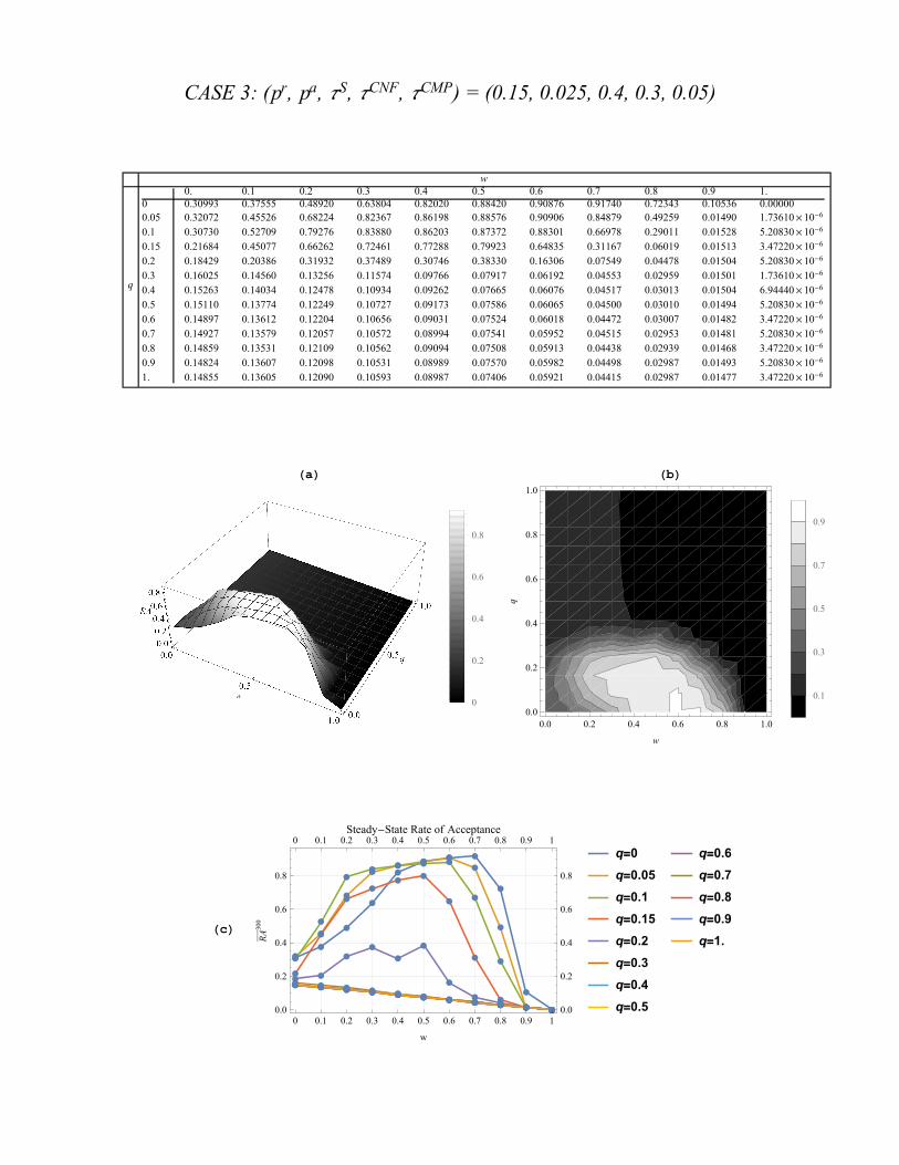
CASE 3: (pr, pa, τS, τCNF, τCMP) = (0.15, 0.025, 0.4, 0.3, 0.05)
w
q
0. 0.1 0.2 0.3 0.4 0.5 0.6 0.7 0.8 0.9 1.0 0.30993 0.37555 0.48920 0.63804 0.82020 0.88420 0.90876 0.91740 0.72343 0.10536 0.000000.05 0.32072 0.45526 0.68224 0.82367 0.86198 0.88576 0.90906 0.84879 0.49259 0.01490 1.73610×10⁻⁶
0.1 0.30730 0.52709 0.79276 0.83880 0.86203 0.87372 0.88301 0.66978 0.29011 0.01528 5.20830×10⁻⁶
0.15 0.21684 0.45077 0.66262 0.72461 0.77288 0.79923 0.64835 0.31167 0.06019 0.01513 3.47220×10⁻⁶
0.2 0.18429 0.20386 0.31932 0.37489 0.30746 0.38330 0.16306 0.07549 0.04478 0.01504 5.20830×10⁻⁶
0.3 0.16025 0.14560 0.13256 0.11574 0.09766 0.07917 0.06192 0.04553 0.02959 0.01501 1.73610×10⁻⁶
0.4 0.15263 0.14034 0.12478 0.10934 0.09262 0.07665 0.06076 0.04517 0.03013 0.01504 6.94440×10⁻⁶
0.5 0.15110 0.13774 0.12249 0.10727 0.09173 0.07586 0.06065 0.04500 0.03010 0.01494 5.20830×10⁻⁶
0.6 0.14897 0.13612 0.12204 0.10656 0.09031 0.07524 0.06018 0.04472 0.03007 0.01482 3.47220×10⁻⁶
0.7 0.14927 0.13579 0.12057 0.10572 0.08994 0.07541 0.05952 0.04515 0.02953 0.01481 5.20830×10⁻⁶
0.8 0.14859 0.13531 0.12109 0.10562 0.09094 0.07508 0.05913 0.04438 0.02939 0.01468 3.47220×10⁻⁶
0.9 0.14824 0.13607 0.12098 0.10531 0.08989 0.07570 0.05982 0.04498 0.02987 0.01493 5.20830×10⁻⁶
1. 0.14855 0.13605 0.12090 0.10593 0.08987 0.07406 0.05921 0.04415 0.02987 0.01477 3.47220×10⁻⁶
(a) (b)
0
0.2
0.4
0.6
0.8
0.0 0.2 0.4 0.6 0.8 1.00.0
0.2
0.4
0.6
0.8
1.0
w
q
0.1
0.3
0.5
0.7
0.9
(c)
0 0.1 0.2 0.3 0.4 0.5 0.6 0.7 0.8 0.9 10.0
0.2
0.4
0.6
0.8
0 0.1 0.2 0.3 0.4 0.5 0.6 0.7 0.8 0.9 1
0.0
0.2
0.4
0.6
0.8
w
RA
300
Steady-State Rate of Acceptance
q=0
q=0.05
q=0.1
q=0.15
q=0.2
q=0.3
q=0.4
q=0.5
q=0.6
q=0.7
q=0.8
q=0.9
q=1.
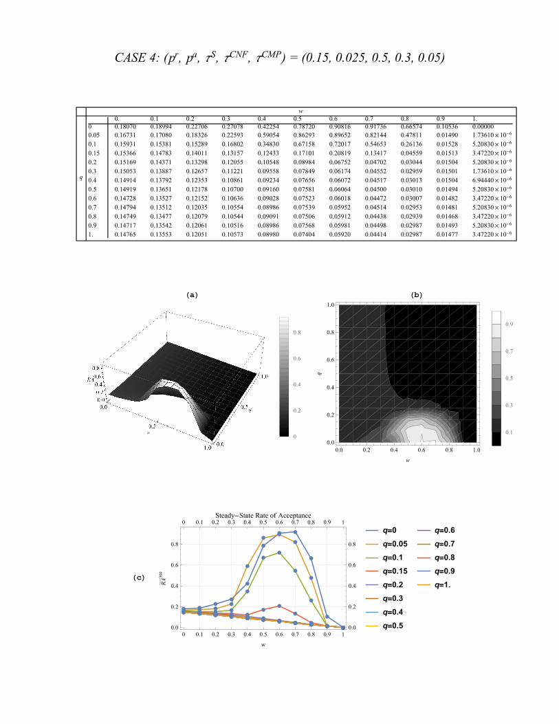
CASE 4: (pr, pa, τS, τCNF, τCMP) = (0.15, 0.025, 0.5, 0.3, 0.05)
w
q
0. 0.1 0.2 0.3 0.4 0.5 0.6 0.7 0.8 0.9 1.0 0.18070 0.18994 0.22706 0.27078 0.42254 0.78720 0.90816 0.91736 0.66574 0.10536 0.000000.05 0.16731 0.17080 0.18326 0.22593 0.59054 0.86293 0.89652 0.82144 0.47811 0.01490 1.73610×10⁻⁶
0.1 0.15931 0.15381 0.15289 0.16802 0.34830 0.67158 0.72017 0.54653 0.26136 0.01528 5.20830×10⁻⁶
0.15 0.15366 0.14783 0.14011 0.13157 0.12433 0.17101 0.20819 0.13417 0.04559 0.01513 3.47220×10⁻⁶
0.2 0.15169 0.14371 0.13298 0.12055 0.10548 0.08984 0.06752 0.04702 0.03044 0.01504 5.20830×10⁻⁶
0.3 0.15053 0.13887 0.12657 0.11221 0.09558 0.07849 0.06174 0.04552 0.02959 0.01501 1.73610×10⁻⁶
0.4 0.14914 0.13792 0.12353 0.10861 0.09234 0.07656 0.06072 0.04517 0.03013 0.01504 6.94440×10⁻⁶
0.5 0.14919 0.13651 0.12178 0.10700 0.09160 0.07581 0.06064 0.04500 0.03010 0.01494 5.20830×10⁻⁶
0.6 0.14728 0.13527 0.12152 0.10636 0.09028 0.07523 0.06018 0.04472 0.03007 0.01482 3.47220×10⁻⁶
0.7 0.14794 0.13512 0.12035 0.10554 0.08986 0.07539 0.05952 0.04514 0.02953 0.01481 5.20830×10⁻⁶
0.8 0.14749 0.13477 0.12079 0.10544 0.09091 0.07506 0.05912 0.04438 0.02939 0.01468 3.47220×10⁻⁶
0.9 0.14717 0.13542 0.12061 0.10516 0.08986 0.07568 0.05981 0.04498 0.02987 0.01493 5.20830×10⁻⁶
1. 0.14765 0.13553 0.12051 0.10573 0.08980 0.07404 0.05920 0.04414 0.02987 0.01477 3.47220×10⁻⁶
(a) (b)
0
0.2
0.4
0.6
0.8
0.0 0.2 0.4 0.6 0.8 1.00.0
0.2
0.4
0.6
0.8
1.0
w
q
0.1
0.3
0.5
0.7
0.9
(c)
0 0.1 0.2 0.3 0.4 0.5 0.6 0.7 0.8 0.9 10.0
0.2
0.4
0.6
0.8
0 0.1 0.2 0.3 0.4 0.5 0.6 0.7 0.8 0.9 1
0.0
0.2
0.4
0.6
0.8
w
RA
300
Steady-State Rate of Acceptance
q=0
q=0.05
q=0.1
q=0.15
q=0.2
q=0.3
q=0.4
q=0.5
q=0.6
q=0.7
q=0.8
q=0.9
q=1.

CASE 5: (pr, pa, τS, τCNF, τCMP) = (0.25, 0, 0.4, 0.3, 0.05)
w
q
0. 0.1 0.2 0.3 0.4 0.5 0.6 0.7 0.8 0.9 1.0 0.55652 0.63791 0.72210 0.80082 0.85603 0.88513 0.90926 0.93126 0.95401 0.63530 0.000010.05 0.65434 0.73661 0.79789 0.83645 0.86226 0.88506 0.90872 0.93156 0.95415 0.41226 8.68060×10⁻⁶
0.1 0.73478 0.78061 0.81250 0.83916 0.86344 0.88511 0.90839 0.93103 0.92614 0.17424 0.000020.15 0.75971 0.79050 0.81576 0.84003 0.86214 0.88548 0.90832 0.93132 0.81348 0.07029 0.000020.2 0.76630 0.79225 0.81655 0.83961 0.86266 0.88479 0.90937 0.90499 0.43331 0.02560 0.000020.3 0.76947 0.79268 0.81719 0.84002 0.86264 0.88605 0.87216 0.27410 0.05186 0.02541 0.000030.4 0.77013 0.79458 0.81664 0.83923 0.86295 0.70339 0.13991 0.07921 0.05138 0.02517 0.000040.5 0.74729 0.79340 0.81702 0.81895 0.57901 0.14734 0.11007 0.07787 0.05035 0.02481 0.000030.6 0.70946 0.79366 0.79893 0.68621 0.22744 0.14136 0.10745 0.07780 0.05089 0.02462 0.000050.7 0.65712 0.72056 0.78012 0.56996 0.19182 0.13915 0.10644 0.07705 0.05071 0.02482 0.000020.8 0.66446 0.71130 0.68255 0.48996 0.17541 0.13734 0.10678 0.07781 0.05110 0.02498 0.000030.9 0.68650 0.72894 0.64777 0.45235 0.17609 0.13775 0.10601 0.07745 0.05056 0.02487 0.000041. 0.60324 0.73487 0.70082 0.41578 0.17702 0.13713 0.10568 0.07747 0.05001 0.02464 0.00005
(a) (b)
0
0.2
0.4
0.6
0.8
0.0 0.2 0.4 0.6 0.8 1.00.0
0.2
0.4
0.6
0.8
1.0
w
q
0.1
0.3
0.5
0.7
0.9
(c)
0 0.1 0.2 0.3 0.4 0.5 0.6 0.7 0.8 0.9 10.0
0.2
0.4
0.6
0.8
1.00 0.1 0.2 0.3 0.4 0.5 0.6 0.7 0.8 0.9 1
0.0
0.2
0.4
0.6
0.8
1.0
w
RA
300
Steady-State Rate of Acceptance
q=0
q=0.05
q=0.1
q=0.15
q=0.2
q=0.3
q=0.4
q=0.5
q=0.6
q=0.7
q=0.8
q=0.9
q=1.
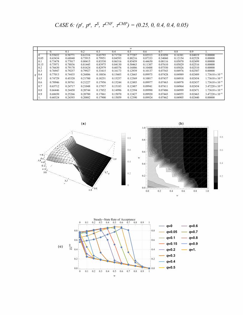
CASE 6: (pr, pa, τS, τCNF, τCMP) = (0.25, 0, 0.4, 0.4, 0.05)
w
q
0. 0.1 0.2 0.3 0.4 0.5 0.6 0.7 0.8 0.9 1.0 0.55652 0.58771 0.61316 0.65793 0.71724 0.77287 0.85513 0.81050 0.16381 0.04019 0.000000.05 0.65434 0.68840 0.73915 0.79951 0.84593 0.88216 0.87333 0.34060 0.12154 0.02528 0.000000.1 0.73478 0.77017 0.80415 0.83530 0.86316 0.85459 0.44650 0.08116 0.05070 0.02499 0.000000.15 0.75971 0.78836 0.81445 0.83975 0.84130 0.50463 0.11307 0.07610 0.05029 0.02516 0.000000.2 0.76630 0.79178 0.81624 0.82979 0.60376 0.16886 0.10488 0.07550 0.05026 0.02510 0.000000.3 0.76947 0.79257 0.79927 0.33415 0.16173 0.12939 0.10137 0.07543 0.04976 0.02507 0.000000.4 0.77013 0.74435 0.26886 0.18836 0.15603 0.12665 0.09975 0.07428 0.04989 0.02489 1.73610×10⁻⁶
0.5 0.74729 0.45320 0.21700 0.18251 0.15257 0.12569 0.10017 0.07437 0.04918 0.02454 1.73610×10⁻⁶
0.6 0.70946 0.30761 0.21227 0.17956 0.15244 0.12485 0.09977 0.07463 0.04978 0.02437 1.73610×10⁻⁶
0.7 0.65712 0.24717 0.21048 0.17937 0.15183 0.12487 0.09941 0.07411 0.04964 0.02454 3.47220×10⁻⁶
0.8 0.66446 0.24450 0.20744 0.17852 0.14996 0.12394 0.09990 0.07486 0.04999 0.02471 1.73610×10⁻⁶
0.9 0.68650 0.25266 0.20780 0.17861 0.15070 0.12427 0.09920 0.07443 0.04955 0.02463 3.47220×10⁻⁶
1. 0.60324 0.24393 0.20882 0.17900 0.15059 0.12390 0.09924 0.07462 0.04905 0.02440 0.00000
(a) (b)
0
0.2
0.4
0.6
0.8
0.0 0.2 0.4 0.6 0.8 1.00.0
0.2
0.4
0.6
0.8
1.0
w
q
0.2
0.4
0.6
0.8
(c)
0 0.1 0.2 0.3 0.4 0.5 0.6 0.7 0.8 0.9 10.0
0.2
0.4
0.6
0.8
0 0.1 0.2 0.3 0.4 0.5 0.6 0.7 0.8 0.9 1
0.0
0.2
0.4
0.6
0.8
w
RA
300
Steady-State Rate of Acceptance
q=0
q=0.05
q=0.1
q=0.15
q=0.2
q=0.3
q=0.4
q=0.5
q=0.6
q=0.7
q=0.8
q=0.9
q=1.
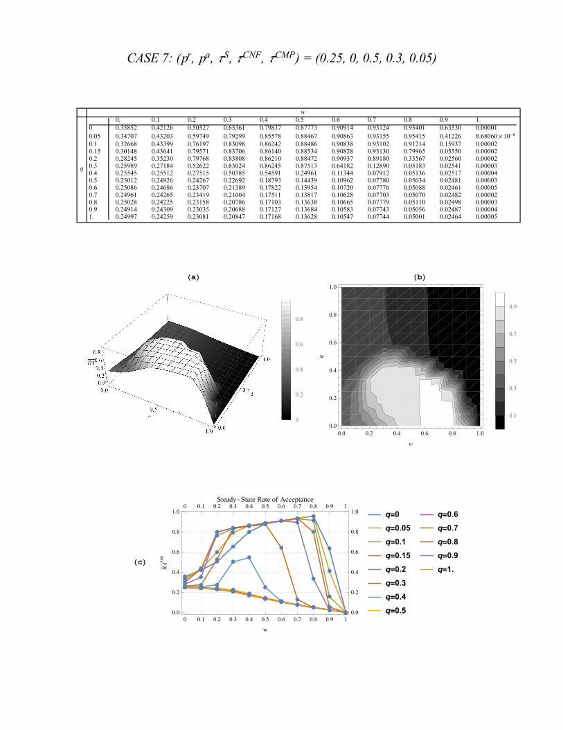
CASE 7: (pr, pa, τS, τCNF, τCMP) = (0.25, 0, 0.5, 0.3, 0.05)
w
q
0. 0.1 0.2 0.3 0.4 0.5 0.6 0.7 0.8 0.9 1.0 0.35852 0.42126 0.50527 0.65361 0.79837 0.87773 0.90914 0.93124 0.95401 0.63530 0.000010.05 0.34707 0.43203 0.59749 0.79299 0.85578 0.88467 0.90863 0.93155 0.95415 0.41226 8.68060×10⁻⁶
0.1 0.32668 0.43399 0.76197 0.83098 0.86242 0.88486 0.90838 0.93102 0.91214 0.15937 0.000020.15 0.30148 0.43641 0.79571 0.83706 0.86140 0.88534 0.90828 0.93130 0.79965 0.05550 0.000020.2 0.28245 0.35230 0.79768 0.83808 0.86210 0.88472 0.90937 0.89180 0.33567 0.02560 0.000020.3 0.25989 0.27184 0.52622 0.83024 0.86245 0.87513 0.64182 0.12890 0.05183 0.02541 0.000030.4 0.25545 0.25512 0.27515 0.50385 0.54591 0.24961 0.11344 0.07912 0.05136 0.02517 0.000040.5 0.25012 0.24926 0.24267 0.22692 0.18793 0.14439 0.10962 0.07780 0.05034 0.02481 0.000030.6 0.25086 0.24686 0.23707 0.21389 0.17822 0.13954 0.10720 0.07776 0.05088 0.02461 0.000050.7 0.24961 0.24265 0.23419 0.21004 0.17511 0.13817 0.10628 0.07703 0.05070 0.02482 0.000020.8 0.25028 0.24225 0.23158 0.20786 0.17103 0.13638 0.10665 0.07779 0.05110 0.02498 0.000030.9 0.24914 0.24309 0.23035 0.20688 0.17127 0.13684 0.10583 0.07743 0.05056 0.02487 0.000041. 0.24997 0.24259 0.23081 0.20847 0.17168 0.13628 0.10547 0.07744 0.05001 0.02464 0.00005
(a) (b)
0
0.2
0.4
0.6
0.8
0.0 0.2 0.4 0.6 0.8 1.00.0
0.2
0.4
0.6
0.8
1.0
w
q
0.1
0.3
0.5
0.7
0.9
(c)
0 0.1 0.2 0.3 0.4 0.5 0.6 0.7 0.8 0.9 10.0
0.2
0.4
0.6
0.8
1.00 0.1 0.2 0.3 0.4 0.5 0.6 0.7 0.8 0.9 1
0.0
0.2
0.4
0.6
0.8
1.0
w
RA
300
Steady-State Rate of Acceptance
q=0
q=0.05
q=0.1
q=0.15
q=0.2
q=0.3
q=0.4
q=0.5
q=0.6
q=0.7
q=0.8
q=0.9
q=1.
CASE 8: (pr, pa, τS, τCNF, τCMP) = (0.25, 0.025, 0.4, 0.3, 0.05)
w
q
0. 0.1 0.2 0.3 0.4 0.5 0.6 0.7 0.8 0.9 1.0 0.55652 0.63946 0.72370 0.80371 0.85660 0.88532 0.90850 0.93136 0.95434 0.56099 0.000020.05 0.65004 0.73233 0.79887 0.83637 0.86231 0.88564 0.90900 0.93185 0.95481 0.26363 0.000020.1 0.72811 0.78072 0.81328 0.83909 0.86365 0.88570 0.90786 0.93163 0.91239 0.17434 0.000030.15 0.75956 0.78935 0.81549 0.83959 0.86236 0.88490 0.90830 0.93173 0.78507 0.07009 0.000030.2 0.76588 0.79279 0.81610 0.83991 0.86346 0.88570 0.90859 0.93109 0.47603 0.02525 0.000020.3 0.76916 0.79380 0.81713 0.84042 0.86274 0.88570 0.84668 0.29969 0.05198 0.02522 0.000020.4 0.76989 0.79397 0.81697 0.83927 0.85289 0.63815 0.11568 0.08006 0.05128 0.02515 0.000020.5 0.76273 0.79437 0.81680 0.84003 0.56909 0.14822 0.10854 0.07790 0.05109 0.02509 0.000010.6 0.74844 0.79387 0.77090 0.71478 0.19507 0.14206 0.10724 0.07755 0.05045 0.02494 0.000020.7 0.66365 0.76087 0.78133 0.57864 0.19197 0.13989 0.10511 0.07730 0.05067 0.02497 0.000030.8 0.67934 0.71929 0.76431 0.55145 0.18944 0.13990 0.10517 0.07715 0.05027 0.02498 0.000030.9 0.68884 0.72859 0.71039 0.44858 0.17570 0.13838 0.10613 0.07704 0.05062 0.02491 0.000011. 0.67126 0.73641 0.75468 0.42420 0.17524 0.13957 0.10619 0.07664 0.05050 0.02482 0.00003
(a) (b)
0
0.2
0.4
0.6
0.8
0.0 0.2 0.4 0.6 0.8 1.00.0
0.2
0.4
0.6
0.8
1.0
w
q
0.1
0.3
0.5
0.7
0.9
(c)
0 0.1 0.2 0.3 0.4 0.5 0.6 0.7 0.8 0.9 10.0
0.2
0.4
0.6
0.8
1.00 0.1 0.2 0.3 0.4 0.5 0.6 0.7 0.8 0.9 1
0.0
0.2
0.4
0.6
0.8
1.0
w
RA
300
Steady-State Rate of Acceptance
q=0
q=0.05
q=0.1
q=0.15
q=0.2
q=0.3
q=0.4
q=0.5
q=0.6
q=0.7
q=0.8
q=0.9
q=1.
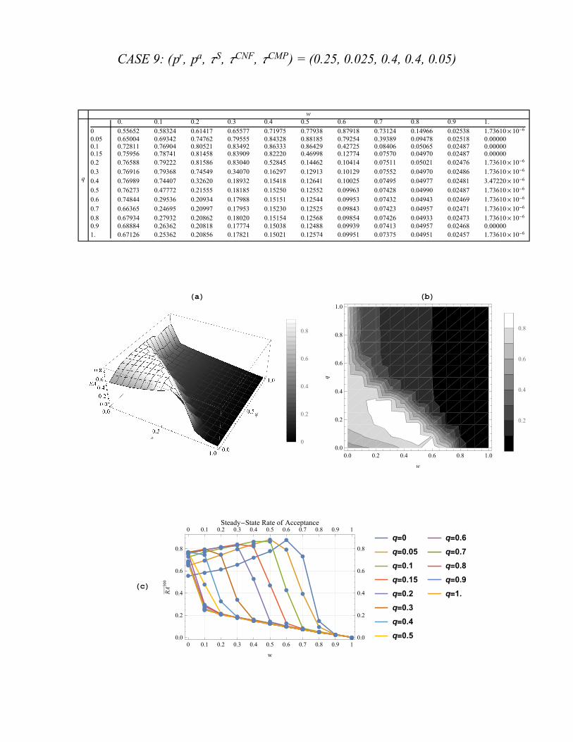
CASE 9: (pr, pa, τS, τCNF, τCMP) = (0.25, 0.025, 0.4, 0.4, 0.05)
w
q
0. 0.1 0.2 0.3 0.4 0.5 0.6 0.7 0.8 0.9 1.
0 0.55652 0.58324 0.61417 0.65577 0.71975 0.77938 0.87918 0.73124 0.14966 0.02538 1.73610×10⁻⁶
0.05 0.65004 0.69342 0.74762 0.79555 0.84328 0.88185 0.79254 0.39389 0.09478 0.02518 0.000000.1 0.72811 0.76904 0.80521 0.83492 0.86333 0.86429 0.42725 0.08406 0.05065 0.02487 0.000000.15 0.75956 0.78741 0.81458 0.83909 0.82220 0.46998 0.12774 0.07570 0.04970 0.02487 0.000000.2 0.76588 0.79222 0.81586 0.83040 0.52845 0.14462 0.10414 0.07511 0.05021 0.02476 1.73610×10⁻⁶
0.3 0.76916 0.79368 0.74549 0.34070 0.16297 0.12913 0.10129 0.07552 0.04970 0.02486 1.73610×10⁻⁶
0.4 0.76989 0.74407 0.32620 0.18932 0.15418 0.12641 0.10025 0.07495 0.04977 0.02481 3.47220×10⁻⁶
0.5 0.76273 0.47772 0.21555 0.18185 0.15250 0.12552 0.09963 0.07428 0.04990 0.02487 1.73610×10⁻⁶
0.6 0.74844 0.29536 0.20934 0.17988 0.15151 0.12544 0.09953 0.07432 0.04943 0.02469 1.73610×10⁻⁶
0.7 0.66365 0.24695 0.20997 0.17953 0.15230 0.12525 0.09843 0.07423 0.04957 0.02471 1.73610×10⁻⁶
0.8 0.67934 0.27932 0.20862 0.18020 0.15154 0.12568 0.09854 0.07426 0.04933 0.02473 1.73610×10⁻⁶
0.9 0.68884 0.26362 0.20818 0.17774 0.15038 0.12488 0.09939 0.07413 0.04957 0.02468 0.000001. 0.67126 0.25362 0.20856 0.17821 0.15021 0.12574 0.09951 0.07375 0.04951 0.02457 1.73610×10⁻⁶
(a) (b)
0
0.2
0.4
0.6
0.8
0.0 0.2 0.4 0.6 0.8 1.00.0
0.2
0.4
0.6
0.8
1.0
w
q
0.2
0.4
0.6
0.8
(c)
0 0.1 0.2 0.3 0.4 0.5 0.6 0.7 0.8 0.9 10.0
0.2
0.4
0.6
0.8
0 0.1 0.2 0.3 0.4 0.5 0.6 0.7 0.8 0.9 1
0.0
0.2
0.4
0.6
0.8
w
RA
300
Steady-State Rate of Acceptance
q=0
q=0.05
q=0.1
q=0.15
q=0.2
q=0.3
q=0.4
q=0.5
q=0.6
q=0.7
q=0.8
q=0.9
q=1.

CASE 10: (pr, pa, τS, τCNF, τCMP) = (0.25, 0.025, 0.5, 0.3, 0.05)
w
q
0. 0.1 0.2 0.3 0.4 0.5 0.6 0.7 0.8 0.9 1.0 0.35852 0.41918 0.51068 0.65509 0.79451 0.87880 0.90821 0.93136 0.95434 0.56099 0.000020.05 0.34776 0.43276 0.60161 0.78733 0.85719 0.88508 0.90894 0.93185 0.95481 0.24879 0.000020.1 0.32690 0.42881 0.76755 0.83124 0.86246 0.88542 0.90783 0.93163 0.91238 0.15949 0.000030.15 0.30195 0.45861 0.80507 0.83692 0.86165 0.88470 0.90829 0.93173 0.72900 0.05522 0.000030.2 0.28138 0.37964 0.80427 0.83837 0.86297 0.88561 0.90858 0.87856 0.33578 0.02525 0.000020.3 0.26148 0.26898 0.43308 0.83995 0.86262 0.84093 0.65150 0.12748 0.05188 0.02522 0.000020.4 0.25556 0.25510 0.26776 0.52386 0.49154 0.25060 0.11382 0.07982 0.05127 0.02515 0.000020.5 0.25168 0.25013 0.24018 0.23480 0.18795 0.14472 0.10819 0.07781 0.05108 0.02509 0.000010.6 0.25028 0.24666 0.23366 0.21400 0.17661 0.14050 0.10703 0.07751 0.05045 0.02494 0.000020.7 0.24881 0.24431 0.23406 0.21024 0.17576 0.13885 0.10497 0.07726 0.05066 0.02497 0.000030.8 0.24877 0.24337 0.23144 0.21080 0.17363 0.13885 0.10493 0.07711 0.05027 0.02498 0.000030.9 0.25126 0.24473 0.23032 0.20524 0.17171 0.13760 0.10598 0.07698 0.05062 0.02491 0.000011. 0.24940 0.24353 0.23073 0.20693 0.17143 0.13878 0.10603 0.07662 0.05050 0.02482 0.00003
(a) (b)
0
0.2
0.4
0.6
0.8
0.0 0.2 0.4 0.6 0.8 1.00.0
0.2
0.4
0.6
0.8
1.0
w
q
0.1
0.3
0.5
0.7
0.9
(c)
0 0.1 0.2 0.3 0.4 0.5 0.6 0.7 0.8 0.9 10.0
0.2
0.4
0.6
0.8
1.00 0.1 0.2 0.3 0.4 0.5 0.6 0.7 0.8 0.9 1
0.0
0.2
0.4
0.6
0.8
1.0
w
RA
300
Steady-State Rate of Acceptance
q=0
q=0.05
q=0.1
q=0.15
q=0.2
q=0.3
q=0.4
q=0.5
q=0.6
q=0.7
q=0.8
q=0.9
q=1.

CASE 11: (pr, pa, τS, τCNF, τCMP) = (0.25, 0.05, 0.5, 0.3, 0.05)
w
q
0. 0.1 0.2 0.3 0.4 0.5 0.6 0.7 0.8 0.9 1.0 0.35852 0.42362 0.51100 0.64237 0.79181 0.87663 0.90810 0.93202 0.95402 0.56056 0.000010.05 0.34671 0.42782 0.60349 0.79033 0.85817 0.88441 0.90879 0.93160 0.92604 0.30824 0.000030.1 0.32212 0.43512 0.76044 0.83342 0.86141 0.88562 0.90832 0.93118 0.94008 0.17408 0.000020.15 0.30342 0.44995 0.80476 0.83815 0.86208 0.88558 0.90893 0.93175 0.65841 0.02538 0.000020.2 0.28104 0.38599 0.80444 0.83970 0.86291 0.88547 0.90844 0.90554 0.27953 0.05551 0.000020.3 0.26237 0.27059 0.56912 0.80321 0.86246 0.86267 0.52103 0.09890 0.05206 0.02534 0.000020.4 0.25374 0.25374 0.26627 0.48670 0.57715 0.19401 0.11524 0.07974 0.05097 0.02520 0.000030.5 0.25116 0.25009 0.24527 0.23527 0.18432 0.14538 0.10884 0.07852 0.05065 0.02528 0.000030.6 0.25001 0.24595 0.23752 0.21102 0.17771 0.13989 0.10751 0.07743 0.05058 0.02500 0.000030.7 0.24970 0.24528 0.23504 0.21058 0.17423 0.13920 0.10627 0.07689 0.05035 0.02480 0.000030.8 0.25001 0.24411 0.23044 0.20692 0.17213 0.13789 0.10682 0.07764 0.05052 0.02497 0.000040.9 0.24791 0.24180 0.22988 0.20860 0.17358 0.13694 0.10684 0.07732 0.05022 0.02504 0.000031. 0.24821 0.24337 0.23105 0.20703 0.17171 0.13704 0.10569 0.07730 0.05034 0.02487 0.00003
(a) (b)
0
0.2
0.4
0.6
0.8
0.0 0.2 0.4 0.6 0.8 1.00.0
0.2
0.4
0.6
0.8
1.0
w
q
0.1
0.3
0.5
0.7
0.9
(c)
0 0.1 0.2 0.3 0.4 0.5 0.6 0.7 0.8 0.9 10.0
0.2
0.4
0.6
0.8
1.00 0.1 0.2 0.3 0.4 0.5 0.6 0.7 0.8 0.9 1
0.0
0.2
0.4
0.6
0.8
1.0
w
RA
300
Steady-State Rate of Acceptance
q=0
q=0.05
q=0.1
q=0.15
q=0.2
q=0.3
q=0.4
q=0.5
q=0.6
q=0.7
q=0.8
q=0.9
q=1.

CASE 12: (pr, pa, τS, τCNF, τCMP) = (0.25, 0.1, 0.5, 0.3, 0.05)
w
q
0. 0.1 0.2 0.3 0.4 0.5 0.6 0.7 0.8 0.9 1.0 0.35860 0.41900 0.51589 0.64924 0.78614 0.87870 0.90803 0.93125 0.95481 0.82842 0.125060.05 0.35208 0.42430 0.60051 0.79504 0.85707 0.88533 0.90817 0.93117 0.95430 0.51642 0.031290.1 0.32290 0.44749 0.76708 0.83315 0.86120 0.88522 0.90797 0.93198 0.95421 0.30806 0.015640.15 0.30126 0.43163 0.80268 0.83596 0.86288 0.88572 0.90853 0.93098 0.82744 0.10014 0.000050.2 0.28224 0.38507 0.79560 0.83795 0.86231 0.88477 0.90863 0.91884 0.43542 0.02605 0.000030.3 0.26291 0.27262 0.44745 0.83116 0.86254 0.88528 0.76440 0.12947 0.05259 0.02496 0.000030.4 0.25556 0.25407 0.27845 0.47122 0.53685 0.25313 0.11686 0.07982 0.05193 0.02503 0.000020.5 0.25143 0.24793 0.24198 0.23727 0.19907 0.14679 0.10911 0.07834 0.05130 0.02520 0.000020.6 0.25010 0.24495 0.23758 0.21574 0.17792 0.14196 0.10720 0.07754 0.05001 0.02505 0.000030.7 0.24983 0.24445 0.23371 0.20914 0.17340 0.13965 0.10587 0.07792 0.05035 0.02493 0.000030.8 0.24861 0.24526 0.23306 0.21001 0.17434 0.13772 0.10579 0.07803 0.05063 0.02498 0.000030.9 0.24937 0.24546 0.23419 0.20865 0.17313 0.13928 0.10683 0.07771 0.05058 0.02500 0.000041. 0.24840 0.24277 0.23092 0.20803 0.17405 0.13849 0.10645 0.07693 0.04980 0.02480 0.00003
(a) (b)
0
0.2
0.4
0.6
0.8
0.0 0.2 0.4 0.6 0.8 1.00.0
0.2
0.4
0.6
0.8
1.0
w
q
0.1
0.3
0.5
0.7
0.9
(c)
0 0.1 0.2 0.3 0.4 0.5 0.6 0.7 0.8 0.9 10.0
0.2
0.4
0.6
0.8
1.00 0.1 0.2 0.3 0.4 0.5 0.6 0.7 0.8 0.9 1
0.0
0.2
0.4
0.6
0.8
1.0
w
RA
300
Steady-State Rate of Acceptance
q=0
q=0.05
q=0.1
q=0.15
q=0.2
q=0.3
q=0.4
q=0.5
q=0.6
q=0.7
q=0.8
q=0.9
q=1.

CASE 13: (pr, pa, τS, τCNF, τCMP) = (0.25, 0.025, 0.4, 0.35, 0.05)
w
q
0. 0.1 0.2 0.3 0.4 0.5 0.6 0.7 0.8 0.9 1.
0 0.55652 0.60790 0.67300 0.74694 0.82493 0.87610 0.90810 0.93136 0.74265 0.06996 1.73610×10⁻⁶
0.05 0.65004 0.71191 0.78140 0.82785 0.86016 0.88539 0.90900 0.90521 0.47494 0.02529 3.47220×10⁻⁶
0.1 0.72811 0.77622 0.81091 0.83841 0.86363 0.88570 0.90786 0.87897 0.24890 0.02499 1.73610×10⁻⁶
0.15 0.75956 0.78861 0.81536 0.83953 0.86235 0.88490 0.85957 0.36509 0.07958 0.02496 6.94440×10⁻⁶
0.2 0.76588 0.79257 0.81606 0.83989 0.86345 0.87504 0.51731 0.10735 0.05072 0.02485 1.73610×10⁻⁶
0.3 0.76916 0.79377 0.81712 0.83072 0.59897 0.19185 0.10585 0.07679 0.05008 0.02490 6.94440×10⁻⁶
0.4 0.76989 0.77718 0.76336 0.38911 0.16653 0.13157 0.10260 0.07585 0.05002 0.02488 3.47220×10⁻⁶
0.5 0.76273 0.74463 0.36681 0.19278 0.15901 0.12897 0.10141 0.07501 0.05009 0.02490 1.73610×10⁻⁶
0.6 0.74844 0.52004 0.23126 0.18872 0.15668 0.12847 0.10105 0.07498 0.04959 0.02473 1.73610×10⁻⁶
0.7 0.66365 0.36681 0.22089 0.18721 0.15706 0.12794 0.09968 0.07479 0.04979 0.02474 6.94440×10⁻⁶
0.8 0.67934 0.38044 0.21954 0.18793 0.15619 0.12836 0.09984 0.07485 0.04948 0.02478 1.73610×10⁻⁶
0.9 0.68884 0.33351 0.21853 0.18477 0.15499 0.12739 0.10066 0.07469 0.04975 0.02471 0.000001. 0.67126 0.37308 0.21873 0.18525 0.15461 0.12833 0.10079 0.07431 0.04966 0.02460 5.20830×10⁻⁶
(a) (b)
0
0.2
0.4
0.6
0.8
0.0 0.2 0.4 0.6 0.8 1.00.0
0.2
0.4
0.6
0.8
1.0
w
q
0.1
0.3
0.5
0.7
0.9
(c)
0 0.1 0.2 0.3 0.4 0.5 0.6 0.7 0.8 0.9 10.0
0.2
0.4
0.6
0.8
0 0.1 0.2 0.3 0.4 0.5 0.6 0.7 0.8 0.9 1
0.0
0.2
0.4
0.6
0.8
w
RA
300
Steady-State Rate of Acceptance
q=0
q=0.05
q=0.1
q=0.15
q=0.2
q=0.3
q=0.4
q=0.5
q=0.6
q=0.7
q=0.8
q=0.9
q=1.

CASE 14: (pr, pa, τS, τCNF, τCMP) = (0.25, 0.025, 0.5, 0.35, 0.05)
w
q
0. 0.1 0.2 0.3 0.4 0.5 0.6 0.7 0.8 0.9 1.
0 0.35852 0.39163 0.43888 0.52009 0.61902 0.77631 0.89802 0.93136 0.65791 0.06996 1.73610×10⁻⁶
0.05 0.34776 0.38310 0.47519 0.61450 0.82051 0.88292 0.90876 0.86606 0.44706 0.02529 3.47220×10⁻⁶
0.1 0.32690 0.36430 0.54935 0.81967 0.86171 0.88540 0.84934 0.57988 0.16453 0.02499 1.73610×10⁻⁶
0.15 0.30195 0.32779 0.57650 0.80302 0.83198 0.77716 0.40449 0.11241 0.05101 0.02496 6.94440×10⁻⁶
0.2 0.28138 0.28355 0.34686 0.41513 0.43768 0.29420 0.13204 0.07837 0.05071 0.02485 1.73610×10⁻⁶
0.3 0.26148 0.24865 0.22931 0.20602 0.17054 0.13575 0.10468 0.07672 0.05007 0.02490 6.94440×10⁻⁶
0.4 0.25556 0.23937 0.21786 0.19105 0.15980 0.13021 0.10235 0.07578 0.05002 0.02488 3.47220×10⁻⁶
0.5 0.25168 0.23590 0.21136 0.18578 0.15695 0.12836 0.10125 0.07497 0.05009 0.02490 1.73610×10⁻⁶
0.6 0.25028 0.23322 0.20837 0.18306 0.15511 0.12790 0.10092 0.07494 0.04959 0.02473 1.73610×10⁻⁶
0.7 0.24881 0.23165 0.20913 0.18251 0.15552 0.12751 0.09957 0.07476 0.04978 0.02474 6.94440×10⁻⁶
0.8 0.24877 0.23089 0.20776 0.18330 0.15465 0.12787 0.09970 0.07483 0.04948 0.02478 1.73610×10⁻⁶
0.9 0.25126 0.23159 0.20712 0.18076 0.15372 0.12698 0.10058 0.07467 0.04974 0.02471 0.000001. 0.24940 0.23122 0.20706 0.18143 0.15341 0.12794 0.10068 0.07429 0.04966 0.02460 5.20830×10⁻⁶
(a) (b)
0
0.2
0.4
0.6
0.8
0.0 0.2 0.4 0.6 0.8 1.00.0
0.2
0.4
0.6
0.8
1.0
w
q
0.1
0.3
0.5
0.7
0.9
(c)
0 0.1 0.2 0.3 0.4 0.5 0.6 0.7 0.8 0.9 10.0
0.2
0.4
0.6
0.8
0 0.1 0.2 0.3 0.4 0.5 0.6 0.7 0.8 0.9 1
0.0
0.2
0.4
0.6
0.8
w
RA
300
Steady-State Rate of Acceptance
q=0
q=0.05
q=0.1
q=0.15
q=0.2
q=0.3
q=0.4
q=0.5
q=0.6
q=0.7
q=0.8
q=0.9
q=1.
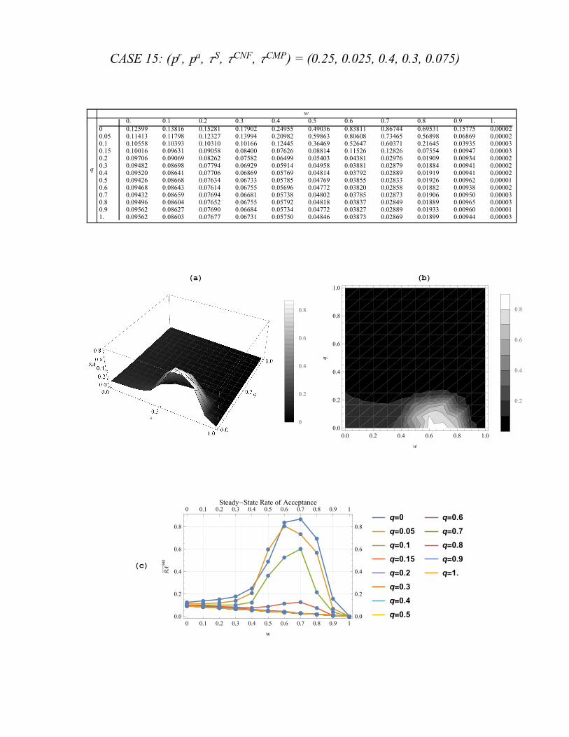
CASE 15: (pr, pa, τS, τCNF, τCMP) = (0.25, 0.025, 0.4, 0.3, 0.075)
w
q
0. 0.1 0.2 0.3 0.4 0.5 0.6 0.7 0.8 0.9 1.0 0.12599 0.13816 0.15281 0.17902 0.24955 0.49036 0.83811 0.86744 0.69531 0.15775 0.000020.05 0.11413 0.11798 0.12327 0.13994 0.20982 0.59863 0.80608 0.73465 0.56898 0.06869 0.000020.1 0.10558 0.10393 0.10310 0.10166 0.12445 0.36469 0.52647 0.60371 0.21645 0.03935 0.000030.15 0.10016 0.09631 0.09058 0.08400 0.07626 0.08814 0.11526 0.12826 0.07554 0.00947 0.000030.2 0.09706 0.09069 0.08262 0.07582 0.06499 0.05403 0.04381 0.02976 0.01909 0.00934 0.000020.3 0.09482 0.08698 0.07794 0.06929 0.05914 0.04958 0.03881 0.02879 0.01884 0.00941 0.000020.4 0.09520 0.08641 0.07706 0.06869 0.05769 0.04814 0.03792 0.02889 0.01919 0.00941 0.000020.5 0.09426 0.08668 0.07634 0.06733 0.05785 0.04769 0.03855 0.02833 0.01926 0.00962 0.000010.6 0.09468 0.08643 0.07614 0.06755 0.05696 0.04772 0.03820 0.02858 0.01882 0.00938 0.000020.7 0.09432 0.08659 0.07694 0.06681 0.05738 0.04802 0.03785 0.02873 0.01906 0.00950 0.000030.8 0.09496 0.08604 0.07652 0.06755 0.05792 0.04818 0.03837 0.02849 0.01889 0.00965 0.000030.9 0.09562 0.08627 0.07690 0.06684 0.05734 0.04772 0.03827 0.02889 0.01933 0.00960 0.000011. 0.09562 0.08603 0.07677 0.06731 0.05750 0.04846 0.03873 0.02869 0.01899 0.00944 0.00003
(a) (b)
0
0.2
0.4
0.6
0.8
0.0 0.2 0.4 0.6 0.8 1.00.0
0.2
0.4
0.6
0.8
1.0
w
q
0.2
0.4
0.6
0.8
(c)
0 0.1 0.2 0.3 0.4 0.5 0.6 0.7 0.8 0.9 10.0
0.2
0.4
0.6
0.8
0 0.1 0.2 0.3 0.4 0.5 0.6 0.7 0.8 0.9 1
0.0
0.2
0.4
0.6
0.8
w
RA
300
Steady-State Rate of Acceptance
q=0
q=0.05
q=0.1
q=0.15
q=0.2
q=0.3
q=0.4
q=0.5
q=0.6
q=0.7
q=0.8
q=0.9
q=1.
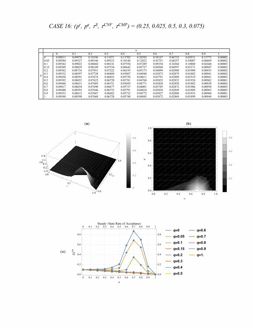
CASE 16: (pr, pa, τS, τCNF, τCMP) = (0.25, 0.025, 0.5, 0.3, 0.075)
w
q
0. 0.1 0.2 0.3 0.4 0.5 0.6 0.7 0.8 0.9 1.0 0.09811 0.09978 0.10196 0.11071 0.13702 0.20395 0.58147 0.86735 0.69531 0.15775 0.000020.05 0.09584 0.09327 0.09146 0.09323 0.10144 0.12822 0.43751 0.68257 0.54087 0.06869 0.000020.1 0.09342 0.09022 0.08668 0.08141 0.07554 0.07289 0.09354 0.34364 0.18880 0.02444 0.000030.15 0.09389 0.08829 0.08149 0.07534 0.06642 0.05727 0.04560 0.04597 0.03371 0.00947 0.000030.2 0.09362 0.08716 0.07951 0.07222 0.06193 0.05173 0.04099 0.02908 0.01909 0.00933 0.000020.3 0.09332 0.08597 0.07728 0.06889 0.05887 0.04940 0.03873 0.02879 0.01882 0.00941 0.000020.4 0.09458 0.08591 0.07674 0.06852 0.05758 0.04811 0.03791 0.02889 0.01919 0.00941 0.000020.5 0.09392 0.08652 0.07625 0.06728 0.05781 0.04768 0.03855 0.02832 0.01926 0.00962 0.000010.6 0.09446 0.08631 0.07605 0.06751 0.05695 0.04771 0.03820 0.02858 0.01882 0.00938 0.000020.7 0.09417 0.08654 0.07690 0.06677 0.05737 0.04801 0.03785 0.02872 0.01906 0.00950 0.000030.8 0.09480 0.08593 0.07646 0.06753 0.05791 0.04818 0.03836 0.02849 0.01889 0.00965 0.000030.9 0.09553 0.08615 0.07687 0.06682 0.05732 0.04772 0.03827 0.02888 0.01933 0.00960 0.000011. 0.09548 0.08598 0.07668 0.06728 0.05748 0.04845 0.03872 0.02869 0.01899 0.00944 0.00003
(a) (b)
0
0.2
0.4
0.6
0.8
0.0 0.2 0.4 0.6 0.8 1.00.0
0.2
0.4
0.6
0.8
1.0
w
q
0.2
0.4
0.6
0.8
(c)
0 0.1 0.2 0.3 0.4 0.5 0.6 0.7 0.8 0.9 10.0
0.2
0.4
0.6
0.8
0 0.1 0.2 0.3 0.4 0.5 0.6 0.7 0.8 0.9 1
0.0
0.2
0.4
0.6
0.8
w
RA
300
Steady-State Rate of Acceptance
q=0
q=0.05
q=0.1
q=0.15
q=0.2
q=0.3
q=0.4
q=0.5
q=0.6
q=0.7
q=0.8
q=0.9
q=1.

Appendix C: Mathematica Code for the Benchmark SimulationThe source code is written using Wolfram Mathematica 10 (version 10.4.1.0). For each parameter configuration,
the computation was distributed among 64 cores, one core for each replication, at the Wharton HPCC (High Perfor-
mance Computing Cluster). The output data were saved and exported for further analysis, the results of which are
presented in this paper.
#!/usr/local/bin/WolframScript -script
myTask=$ScriptCommandLine[[2]];
Print["Running task: ",myTask]
Stigma Project: Base Code for Benchmark SimulationCode created by: Myong-Hun Chang (initial date: 3/8/2016)
Revised: 4/21/2017
SeedRandom[myTask];
Functions
Initialize the Population Grid
population[X_,Y_]:=
(
P=X*Y;
toIndex[n_,m_]:=n-1+(m-1)*X; (* function for transforming (n, m) into a single index number *)
toCoord[x_]:={Mod[x,X]+1,Quotient[x,X]+1}; (* function for transforming an index number into (n, m) coordinates *)
);
code0.nb | 1
6/6/17

Agent Types
typestatus[s_,w_]:=
(
stig=RandomSample[Range[P],IntegerPart[P*s]];
types=ReplacePart[Table[0,{i,1,P}],Subsets[stig,{1}]→1];
comp=RandomSample[Complement[Range[P],stig],Round[(P-Length[stig])*(1-w)]];
types=ReplacePart[types,Subsets[comp,{1}]→2];
Do[type[i]=types[[i+1]],{i,0,P-1}];
ClearAll[types,stig,comp];
);
Agent Neighbors (Torus)
xtbl[a_]:=
(
Which[
(a-R≥1)&&(a+R≤X),
Table[i,{i,a-R,a+R}],
(a-R<1)&&(a+R≤X),
Union[Table[i,{i,1,a+R}],Table[i,{i,X+(a-R),X}]],
(a-R≥1)&&(a+R>X),
Union[Table[i,{i,a-R,X}],Table[i,{i,1,(a+R)-X}]]
]
);
2 | code0.nb
6/6/17
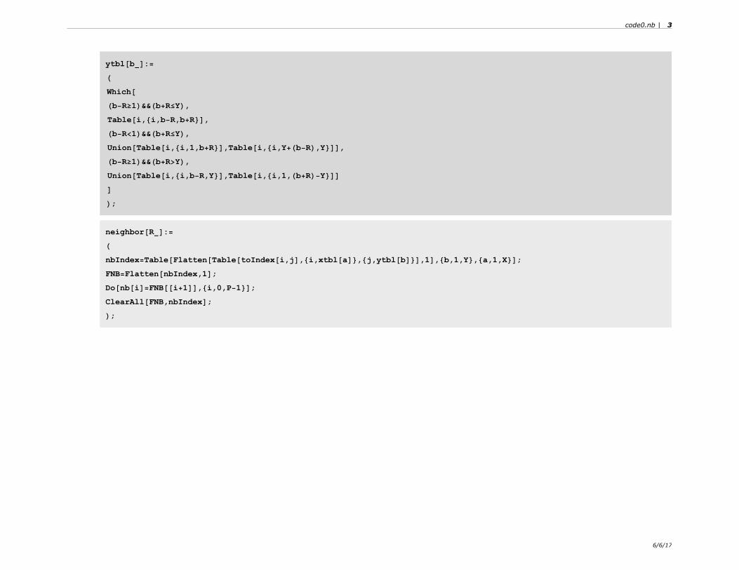
ytbl[b_]:=
(
Which[
(b-R≥1)&&(b+R≤Y),
Table[i,{i,b-R,b+R}],
(b-R<1)&&(b+R≤Y),
Union[Table[i,{i,1,b+R}],Table[i,{i,Y+(b-R),Y}]],
(b-R≥1)&&(b+R>Y),
Union[Table[i,{i,b-R,Y}],Table[i,{i,1,(b+R)-Y}]]
]
);
neighbor[R_]:=
(
nbIndex=Table[Flatten[Table[toIndex[i,j],{i,xtbl[a]},{j,ytbl[b]}],1],{b,1,Y},{a,1,X}];
FNB=Flatten[nbIndex,1];
Do[nb[i]=FNB[[i+1]],{i,0,P-1}];
ClearAll[FNB,nbIndex];
);
code0.nb | 3
6/6/17
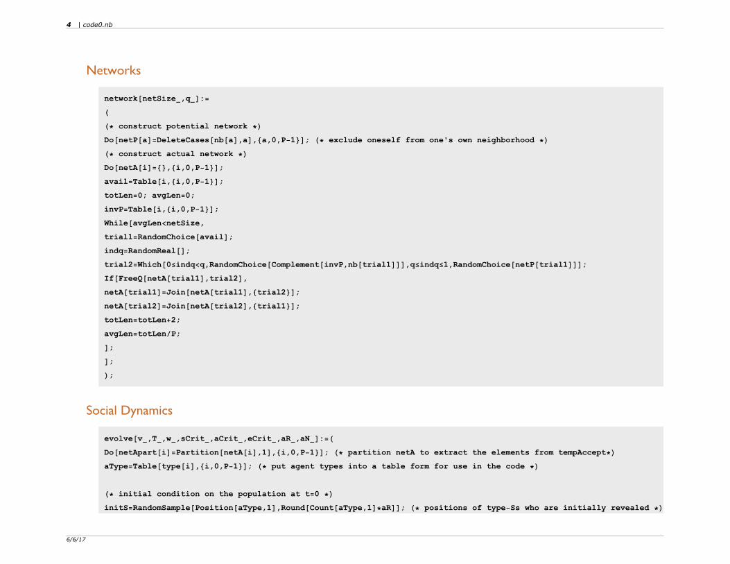
Networks
network[netSize_,q_]:=
(
(* construct potential network *)
Do[netP[a]=DeleteCases[nb[a],a],{a,0,P-1}]; (* exclude oneself from one's own neighborhood *)
(* construct actual network *)
Do[netA[i]={},{i,0,P-1}];
avail=Table[i,{i,0,P-1}];
totLen=0; avgLen=0;
invP=Table[i,{i,0,P-1}];
While[avgLen<netSize,
trial1=RandomChoice[avail];
indq=RandomReal[];
trial2=Which[0≤indq<q,RandomChoice[Complement[invP,nb[trial1]]],q≤indq≤1,RandomChoice[netP[trial1]]];
If[FreeQ[netA[trial1],trial2],
netA[trial1]=Join[netA[trial1],{trial2}];
netA[trial2]=Join[netA[trial2],{trial1}];
totLen=totLen+2;
avgLen=totLen/P;
];
];
);
Social Dynamics
evolve[v_,T_,w_,sCrit_,aCrit_,eCrit_,aR_,aN_]:=(
Do[netApart[i]=Partition[netA[i],1],{i,0,P-1}]; (* partition netA to extract the elements from tempAccept*)
aType=Table[type[i],{i,0,P-1}]; (* put agent types into a table form for use in the code *)
(* initial condition on the population at t=0 *)
initS=RandomSample[Position[aType,1],Round[Count[aType,1]*aR]]; (* positions of type-Ss who are initially revealed *)
4 | code0.nb
6/6/17

initN=RandomSample[Position[aType,0 2],Round[Count[aType,0 2]*aN]]; (* positions of normals initially accepting *)
timeReveal[0]=ReplacePart[Table[-1,{i,1,P}],initS→1]; (* type S initially revealed; everyone else hidden *)
timeAccept[0]=ReplacePart[Table[0,{i,1,P}],Union[initS,initN]→1]; (* all initially accepting; others neutral *)
Do[rho[i]=Which[type[i]⩵1,sCrit,type[i]⩵0,aCrit,type[i]⩵2,eCrit],{i,0,P-1}]; (* assign thresholds *)
Do[
popReveal=Count[timeReveal[t-1],1]; (* no. revealed agents in the global population *)
popAccept=Count[timeAccept[t-1],1]; (* no. accepting agents in the global population *)
Do[
If[netA[i]⩵{},
propA[i]=0;
propR[i]=0;
,
propA[i]=Count[Extract[timeAccept[t-1],netApart[i]+1],1]/Length[netA[i]];
propR[i]=Count[Extract[timeReveal[t-1],netApart[i]+1],1]/Length[netA[i]];
]
,{i,0,P-1}]; (* compute the proportion of an agent's network who are accepting/revealed *)
(* decision making by the stigmatized (S) - type 1 : switch from (N,H) to (A,R) iff ait-1≥τS *)
tempReveal=ReplacePart[timeReveal[t-1],Intersection[Position[aType,1],
Position[timeReveal[t-1],-1],
Position[Table[propA[i]-rho[i],{i,0,P-1}],n_/;n≥0]]->1];
tempAccept=ReplacePart[timeAccept[t-1],Intersection[Position[aType,1],
Position[timeAccept[t-1],0],
Position[Table[propA[i]-rho[i],{i,0,P-1}],n_/;n≥0]]→1];
(* decision making by the conformists (CNF) - type 0 *)
(* go to (O,H) if ait-1<τCNF : oppose *)
tempAccept=ReplacePart[tempAccept,Intersection[Position[aType,0],
Position[Table[propA[i]-rho[i],{i,0,P-1}],n_/;n<0]]→-1];
(* go to (A,H) if ait-1≥τCNF : accept *)
code0.nb | 5
6/6/17

tempAccept=ReplacePart[tempAccept,Intersection[Position[aType,0],
Position[Table[propA[i]-rho[i],{i,0,P-1}],n_/;n≥0]]→1];
(* decision making by the compassionists (CMP) - type 2 *)
(* go to (N,H) if rit-1<τCMP : neutral *)
tempAccept=ReplacePart[tempAccept,Intersection[Position[aType,2],
Position[Table[propR[i]-rho[i],{i,0,P-1}],n_/;n<0]]→0];
(* go to (A,H) if rit-1≥τCMP : accept *)
tempAccept=ReplacePart[tempAccept,Intersection[Position[aType,2],
Position[Table[propR[i]-rho[i],{i,0,P-1}],n_/;n≥0]]→1];
(* update the individual status *)
timeReveal[t]=tempReveal;
timeAccept[t]=tempAccept;
(* update the population state *)
timePropA[t-1]=Table[propA[i],{i,0,P-1}];
timePropR[t-1]=Table[propR[i],{i,0,P-1}];
,{t,1,T}];
);
Parameter Configuration
6 | code0.nb
6/6/17

dx=0; (* dataset index *)
w=0.8; (* proportion of the "normal" population who are conformists *)
X=100;Y=100; (* dimensions of the population grid *)
s=0.1; (* proportion of the population who are stigmatized *)
q=0; (* probability of an agent's link being from outside his neighborhood (nb) *)
R=3; (* range of the Moore neighborhood for network construction *)
netSize=20; (* mean size of the actual network *)
v=1; (* proportion of the population who update their status each period *)
T=300; (* time horizon *)
aR=0.15; (* fraction of the stigmatized who are revealed at t=0 *)
aN=0; (* fraction of the normals who are revealed at t=0 *)
sCrit=0.4; (* threshold to reveal by a stigmatized *)
aCrit=0.3; (* threshold to accept by a conformist *)
eCrit=0.05; (* threshold to accept by a compassionist *)
REP=1; (* no. replications *)
Simulate
(* call the functions *)
population[X,Y];
neighbor[R];
(* initialize data collection *)
pNormA={};
pNormO={};
pNormN={};
pStigR={};
numNormA={};
numConfA={};
numCompA={};
code0.nb | 7
6/6/17

(* initialize network composition *)
popType={};
popNetSize={};
popNumS={};
popPropS={};
ssAccept={};
ssReveal={};
LCC={};
GCC={};
Do[
network[netSize,q];
(* network statistics *)
inetSize=Table[Length[netA[i]],{i,0,P-1}]; (* i's network size *)
popNetSize=Append[popNetSize,inetSize];
comNet=Table[Map[UndirectedEdge[i,#]&,netA[i]],{i,0,X*Y-1}];
(* compute the clustering coefficient *)
LCC=Append[LCC,Mean[LocalClusteringCoefficient[Flatten[comNet]]]//N];
GCC=Append[GCC,GlobalClusteringCoefficient[Flatten[comNet]]//N];
Do[
typestatus[s,w];
evolve[v,T,w,sCrit,aCrit,eCrit,aR,aN];
(* compute and save*)
numReveal=Table[Count[timeReveal[t],1],{t,0,T}];
numAccept=Table[Count[timeAccept[t],1],{t,0,T}];
numNeutral=Table[Count[timeAccept[t],0],{t,0,T}];
numOppose=Table[Count[timeAccept[t],-1],{t,0,T}];
8 | code0.nb
6/6/17
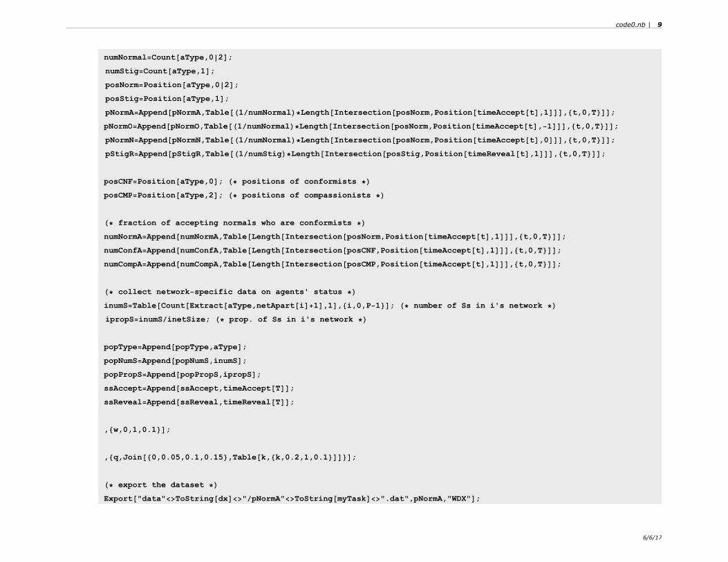
numNormal=Count[aType,0 2];
numStig=Count[aType,1];
posNorm=Position[aType,0 2];
posStig=Position[aType,1];
pNormA=Append[pNormA,Table[(1/numNormal)*Length[Intersection[posNorm,Position[timeAccept[t],1]]],{t,0,T}]];
pNormO=Append[pNormO,Table[(1/numNormal)*Length[Intersection[posNorm,Position[timeAccept[t],-1]]],{t,0,T}]];
pNormN=Append[pNormN,Table[(1/numNormal)*Length[Intersection[posNorm,Position[timeAccept[t],0]]],{t,0,T}]];
pStigR=Append[pStigR,Table[(1/numStig)*Length[Intersection[posStig,Position[timeReveal[t],1]]],{t,0,T}]];
posCNF=Position[aType,0]; (* positions of conformists *)
posCMP=Position[aType,2]; (* positions of compassionists *)
(* fraction of accepting normals who are conformists *)
numNormA=Append[numNormA,Table[Length[Intersection[posNorm,Position[timeAccept[t],1]]],{t,0,T}]];
numConfA=Append[numConfA,Table[Length[Intersection[posCNF,Position[timeAccept[t],1]]],{t,0,T}]];
numCompA=Append[numCompA,Table[Length[Intersection[posCMP,Position[timeAccept[t],1]]],{t,0,T}]];
(* collect network-specific data on agents' status *)
inumS=Table[Count[Extract[aType,netApart[i]+1],1],{i,0,P-1}]; (* number of Ss in i's network *)
ipropS=inumS/inetSize; (* prop. of Ss in i's network *)
popType=Append[popType,aType];
popNumS=Append[popNumS,inumS];
popPropS=Append[popPropS,ipropS];
ssAccept=Append[ssAccept,timeAccept[T]];
ssReveal=Append[ssReveal,timeReveal[T]];
,{w,0,1,0.1}];
,{q,Join[{0,0.05,0.1,0.15},Table[k,{k,0.2,1,0.1}]]}];
(* export the dataset *)
Export["data"<>ToString[dx]<>"/pNormA"<>ToString[myTask]<>".dat",pNormA,"WDX"];
code0.nb | 9
6/6/17

Export["data"<>ToString[dx]<>"/pNormO"<>ToString[myTask]<>".dat",pNormO,"WDX"];
Export["data"<>ToString[dx]<>"/pNormN"<>ToString[myTask]<>".dat",pNormN,"WDX"];
Export["data"<>ToString[dx]<>"/pStigR"<>ToString[myTask]<>".dat",pStigR,"WDX"];
Export["data"<>ToString[dx]<>"/numNormA"<>ToString[myTask]<>".dat",numNormA,"WDX"];
Export["data"<>ToString[dx]<>"/numConfA"<>ToString[myTask]<>".dat",numConfA,"WDX"];
Export["data"<>ToString[dx]<>"/numCompA"<>ToString[myTask]<>".dat",numCompA,"WDX"];
Export["data"<>ToString[dx]<>"/LCC"<>ToString[myTask]<>".dat",LCC,"WDX"];
Export["data"<>ToString[dx]<>"/GCC"<>ToString[myTask]<>".dat",GCC,"WDX"];
Export["data"<>ToString[dx]<>"/aType"<>ToString[myTask]<>".dat",popType,"WDX"];
Export["data"<>ToString[dx]<>"/inetSize"<>ToString[myTask]<>".dat",popNetSize,"WDX"];
Export["data"<>ToString[dx]<>"/inumS"<>ToString[myTask]<>".dat",popNumS,"WDX"];
Export["data"<>ToString[dx]<>"/ipropS"<>ToString[myTask]<>".dat",popPropS,"WDX"];
Export["data"<>ToString[dx]<>"/ssAccept"<>ToString[myTask]<>".dat",ssAccept,"WDX"];
Export["data"<>ToString[dx]<>"/ssReveal"<>ToString[myTask]<>".dat",ssReveal,"WDX"];
10 | code0.nb
6/6/17


![Theory of Planned Behavior, Self‑Stigma, and Perceived ...file.qums.ac.ir/repository/sdh/Theory of Planned...self-stigma (also known as internalized stigma).[5,6] Self-stigma was](https://img.pdfslide.net/doc/110x75/5f59324ffcada40fd01f4b2a/theory-of-planned-behavior-selfastigma-and-perceived-filequmsacirrepositorysdhtheory.jpg)