The Solution for Optimal Power Flow (OPF) Method Using

IJITEE, Vol. 1, No. 1, March 2017

Hazel Ariantara: The Solution for Optimal ... ISSN 2550-0554 (Online)

1 Student, Dept. of Electrical Engineering and Information

Technology, Faculty of Engineering, Universitas Gadjah Mada, Jl.

Grafika No. 2 Kampus UGM Yogyakarta, 55281 INDONESIA (tlp:

0274-552305; e-mail: [email protected]) 2, 3 Lecturer, Dept. of Electrical Engineering and Information

Technology, Faculty of Engineering, Universitas Gadjah Mada, Jl.

Grafika No. 2 Kampus UGM Yogyakarta, 55281 INDONESIA (tlp:

0274-552305)

The Solution for Optimal Power Flow (OPF) Method Using

Differential Evolution Algorithm Hazel Ariantara1, Sarjiya2, Sasongko Pramono Hadi3

Abstract- Optimal Power Flow (OPF) is one of techniques used

to optimize the cost of power plant production while maintaining

the limit of system reliability. In this paper, the application of

differential evolution (DE) method is used to solve the OPF

problem with variable control such as the power plant output,

bus voltage tension, transformer tap, and injection capacitor.

The effectiveness of the method was tested using IEEE 30 buses.

The result shows that this method is better than generic

algorithm (GA), particle swarm optimized (PSO), fuzzy GA,

fuzzy PSO, and bat-algorithm. The simulation of the power plant

systems of 500 kV Java-Bali with the proposed method can

reduce the total cost of generation by 13.04% compared to the

operating data PT. PLN (Persero).

Keywords– optimal power flow, differential evolution, variable

control

I. INTRODUCTION

The need of electric power progressively increases along

with the development of technology and the increase of

population. It makes the demand for energy continue to rise.

On the other hand, the energy supplied by the generator must

be greater. Generally, to supply the energy, some power plants

that are mutually interconnected are required in order to fulfil

those needs. The utilization of electrical energy without an

accurate calculation can effectively lead to the fuel surplus in

each generating unit. Judging from the fuel consumption, most

of it happens in the thermal power plant. The type of power

plant in Indonesia is a thermal power plant type. In Java-Bali

network, the contribution cost of fuel in the electricity

production is about 60% from the total cost. Because of that,

to reduce the price of electricity, the optimization costs on the

process of electric production needed to be performed. In the

interconnection power system, the optimization cost can be

achieved by controlling the active and reactive power of each

power plant. This method is called optimal power flow (OPF)

[1].

In the OPF, controlled variable is used to minimize the

power plant operational costs. The OPF also has restraints. It

consists of calculating active power limit and reactive power

plant; restrain the power capability from transmission system,

transformer tap, and voltage plan [2].

The OPF analysis has been developed from time to time. It

evolves and becomes an algorithm which is applied

successfully. There are several methods that have been

developed. They are conventional optimization methods, such

as newton method, quadratic programming (QP), linear

programming (LP), and non-linear programming (NLP). It

also occurs in the latest optimization methods, heuristic

methods such as genetic algorithm (GA), particle swarm

optimization (PSO), tabu search (TS), simulated annealing

(SA), evolutionary programming (EP), etc. The conventional

methods have several weaknesses, namely: heavily rely on the

value of the initial guess, difficult to reach convergence, often

getting stuck in optimum value, and relying heavily on the

purpose and restriction of the system in order to optimize the

global value [3]. In addition, the other research shows that the

shortage of GA occurs because of the computing process

which is slow. It occurs because there are many selection

factors that must be processed [4]. Whereas, the PSO

weakness is the possibility of the swarm state and reach the

convergent state prematurely. This is due to the convergent of

the global best particles PSO that is located on the line

between the global best and personal best. At this point, it

does not guarantee the best global solution.

On the previous research, the OPF has been accomplished

using numerous conventional optimization techniques such as

linear programming, non-linear programming, quadratic

programming, newton method, dynamic programming, mixed-

integer programming, decomposition technique, and interior

point method [5] - [12]. The OPF problems were solved using

PSO method. The objective is to minimize the power plant

cost of IEEE 30 bus system. Then, the simulation results were

compared with the gradient and GA method [13]. The

problems also solved via the implementation of enhanced GA

using roulette wheel to test IEEE 30 bus system and IEEE

RTS-96 3-area [14]. In the previous study, OPF problems

were solved using EP method to reduce the cost applied in

IEEE 30 bus system. The simulation showed that EP method

is better GA method. [15]. The hybrid tabu search and

simulated annealing (TS/SA) have been used to minimize the

OPF fuel cost by using multiple types of devices such as

flexible alternating current transmission system (FACTS)

[16]. The test on the IEEE 30 bus systems showed better

results and required a shorter computation time instead of

using GA, TS, or SA. On the other hand, fuzzy integration

system with GA and PSO was used to solve the problems

happened on OPF [17]. The test results on the IEEE 30 bus

system showed it had better solution and was able to cut the

computation time compared to standard methods of GA and

PSO.

19


ISSN 2550-0554 (Online) Hazel Ariantara: The Solution for Optimal ...

Differential evolution (DE) is a new optimization method

based on the evolutionary algorithm with the principles and

philosophy algorithmically mimics the behaviour of biological

evolution. DE can handle complex optimization problem, and

simple coding so that it is easy to use [18]. In this journal, the

DE has been proposed to solve the OPF problem with the

objective to minimize total cost energy that used to generate

electricity. Variable controls that have been used are the

output of active power plants, bus voltage generator,

transformer tap and capacitor injection. The effectiveness test

of this method is performed in the case of IEEE 30 bus system

and 500 kV power system Java-Bali. Then, the simulation

results were compared with the other heuristic methods.

II. OPTIMAL POWER FLOW

The OPF problem is a non-linear optimization problem

with the objective function of non-linear and non-linear

constraints. The OPF problem requires solution of non-linear

equations; describing the optimal or safety operation of the

energy system. OPF problems can be formulated as follows:

Minimization F(x,u) (1)

with the provision G(x,u)=0 (2)

H(x,u) ≤ 0. (3)

where F(x,u) as objective function that will be optimized.

Generally, G(x,u) is the balance of real power equation and

reactive power, while H(x, u) is safety limit. x is dependent

vector that consists of bus active power output with PG1

reference, magnitude voltage at load bus VL, the output of

reactive power plant QG, and the load of transmission line SL.

xT = [PG1,VL, QG, SL] (4)

where u as variable control that consists of the output of active

power generator PG, voltage magnitude at generator bus

including bus reference VG, transformer tap positions T, and

reactive power injection QC.

uT = [PG, VG,T,QC]. (5)

Mathematically the objective function of minimizing the fuel

cost can be formulated as (6).

= (6)

Where F is the total fuel cost generating, , , and is the

coefficient generator fuel , and is the number of

generating units.

A. The Linear Limit

Linear limit G(x,u) is the equation of real force balance and

reactive force that can be expressed as follows.

(7)

(8)

Where,

= the output of active power at bus i

= the output of reactive power at bus i

= the needs of active power bus i

= the needs of reactive power at bus i

= total bus

= the different phase between bus i dan bus j

dan = admittance matrix elements between bus i

dan bus j

B. The Non-linear Limit

Non-linear limit reflects the boundary of security system.

The non-linear equation can be seen as follows.

1) Boundary Plant: Magnitude voltage plant, the output of

active force and reactive power limited by lower and upper

limit are as follows.

≤ ≤ ; i = 1,…, (9)

≤ ≤ ; i = 1,…, (10)

≤ ≤ ; i = 1,…, (11)

2) Boundary Transformer: Transformer tap settings

limited by the lower and upper limit are as follows.

≤ ≤ ; i = 1,…, . (12)

3) Boundary Compensator VAR: Reactive force injection

on the bus limited by the lower and upper limit is as follows.

≤ ≤ ; i = 1,…, (13)

4) Boundary Security: Boundary security system includes

the magnitude of the voltage on each bus and transmission

line charge. Systematically, boundary security can be

formulated as follows.

≤ ≤ ; i = 1,…, (14)

≤ ; i = 1,…, (15)

III. DIFFERENTIAL EVOLUTION

DE is a method introduced by Kenneth Price and Rainer

Storn in 1995 [19]. It is a multidimensional function of

mathematical optimization method and the global

optimization algorithm within evolution based. The idea of

this algorithm is to presume the individual as a vector.

Individual modification on mutation and re-combination is

performed through the summation and subtraction of vector

operations [20]. Along with the development, the DE becomes

one of the best genetic algorithms. It can generate global

optimum multidimensional (more than one optimum value)

with a good probability.

Compared with the previous evolutionary algorithm

method, the advantage of the DE is the presence of evolution

which experienced by each individual in the population with

differentiation and crossover. It occurs randomly and

consecutively in each individual which is selected from the

population every time. If the individual provides smaller value

of function, new individual will replace it. Otherwise, the

individual long maintained [21]. The optimization process is

20



carried out through four basic operations, namely

initialization, mutation, crossover, and selection.

A. Initialization

The algorithm begins from creating vector population

which consists of individuals who evolve in each

iterations/generations g. Each individual represents quantity

vector that contains various elements of problem. The first

step is to create an initial population from solution candidate

by generating random values from each of them, which are

upper and lower limit of each specified parameter. Generally,

uniform distribution is used to generate the random number

initialization because it is able to overcome the lack of

information at the optimal point. The probability of uniform

distribution from the random variable can be seen from the

following equation.

xj,i,0 = rand j (bj, maks – bj, min) + bj, min (16)

where

xj,i,0 = the initial value parameter –j with g=0 from

vector i

rand j = random numbers of uniform distribution from

range [0,1]

bj, maks = upper limit

bj, min = lower limit

B. Mutation

After initialized, DE will mutate and re-combine the initial

population to generate a new population. In the genetic

context, mutation can be defined as the change of random

elements. To control the mutation and improve convergence,

deferential vector is scaled by a constant range [0,2], which is

called F constant (scaling factor). The (17) equation showing

on how to form a mutant vector, vi,g.

vi,g = x r0,g + F. (x r1,g – x r2,g ) (17)

where r0, r1, r2 are random indices, integers, and they must

be different from others. Vector base index, Vector base

index, r0, can be specified from various ways, such as

random, permutation, stochastic, and random offset. Whereas,

r1 and r2 are randomly selected from each mutation.

C. Crossover

To complete the search strategy, the DE uses crossover

operation. The aim of crossover operation is to increase the

diversity of the population parameter. Crossover generates

vector test (trial vectors) from the value parameter that have

been copied from two different vectors. The vector equation

test can be seen as follow.

(18)

where

rand j = random uniform distribution with range [0, 1]

Cr = constant crossover specified by consumer

u i,g = test vector

v i,g = mutation vector

x i,g = target vector.

The function of Cr is to control the refraction values of the

parameters which are copied from the mutation. The test

parameter that randomly selected index jrand is taken from

mutations to ensure that the test vectors do not duplicate x i,g.

D. Selection

Selection operator chooses the vector that will compose the

population in the next generation. If test vector has the

same value as objective function or lower than the target

vector , it will replace vector target on the next

generation. On the contrary, the target population will

maintain its position for at least one generation.

(19)

The selection process for each pair of target or vector test

will be repeated until the population from the next generation

complete.

E. Discontinuation Iteration Criteria

After the new population is generated in the selection

process, the process of mutation, recombination, and selection

will be repeated until it reaches an optimal result. In some

cases, reiteration until optimum globalization will take very

long time. That's why the criteria that can stop the iteration

time are needed. The limitations of iteration are as follow:

the value of function at certain stage is reached,

the performance of maximum number of iterations,

statistical provision of a population is approaching at

certain number, and

provision length of time iteration

When the iteration limit is reached, the search for the

optimum point will stop and the vector populations that have

the best value will become the optimal point.

IV. RESULTS AND DISCUSSION

To determine the effectiveness of the OPF, the proposed

method will be tested with the IEEE 30 bus system, before it

was applied in Java-Bali system. This program was created

and developed using Dell laptops Inspiron 1320 Intel®

Core™2 Duo @2.10GHz, 2.00 GB-RAM with Windows 7

and MATLAB software.

A. IEEE 30 Bus System

This system have six generating units with bus 1 as

reference, 30 buses and 41 transmission lines with a total load

of 283.4 MW. This system has 25 control variables, namely

six unit active power plant output, six magnitude bus voltage,

four tap transformer settings, and nine injection capacitors.

The coefficient of power plant costs and limitations of IEEE

30 bus system are shown in Table I [22]. From the simulation

which happened before optimization, DE obtained total cost

860.80 $/hour of power plant with the amount of transmission

21



loss was 14.64 MW. Besides that, there is a violation on the

limitation of the voltage and the transmission line.

In this case, the simulation is done using the following

parameters:

F = 0.5

CR = 0.9

NP = 50

Iteration = 200

The best results in the simulation which is conducted in ten

experiments, are shown in Table II, with the amount of 800.50

$/hour.

TABLE I

THE LIMITATION AND COEFFICIENT OF GENERATING COSTS

No Coefficient Costs PGmin

(MW)

PGmax

(MW) a b c

1 0 2.00 0.00375 50 200

2 0 1.75 0.01750 20 80

3 0 1.00 0.06250 15 50

4 0 3.25 0.00834 10 35

5 0 3.00 0.02500 10 30

6 0 3.00 0.02500 12 40

TABLE II

OPF-DE SIMULATION RESULTS WITH IEEE 30 BUS SYSTEM

Power Plant Load (MW)

P1 177,004

P2 48,715

P3 21,390

P4 21,300

P5 12,006

P6 12,000

Total Cost($/hour) 800,50

Total loses (MW) 9,028

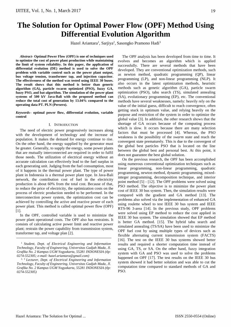
Fig. 1 The total cost of power plant in IEEE 30 bus system.

Fig. 1 shows total power plant cost which the optimal value

could be reached before iterating 100th. From these results,

there was 60.30 $/hour (7%) saving and total of transmission

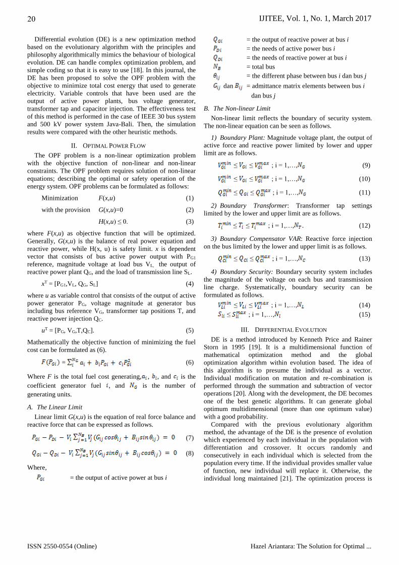
losses is 5.61 MW (38.3%). Moreover, the voltage magnitude

of each bus was still in specified operation limits, with lower

limit provision was (0.95 pu) and upper limit provision was

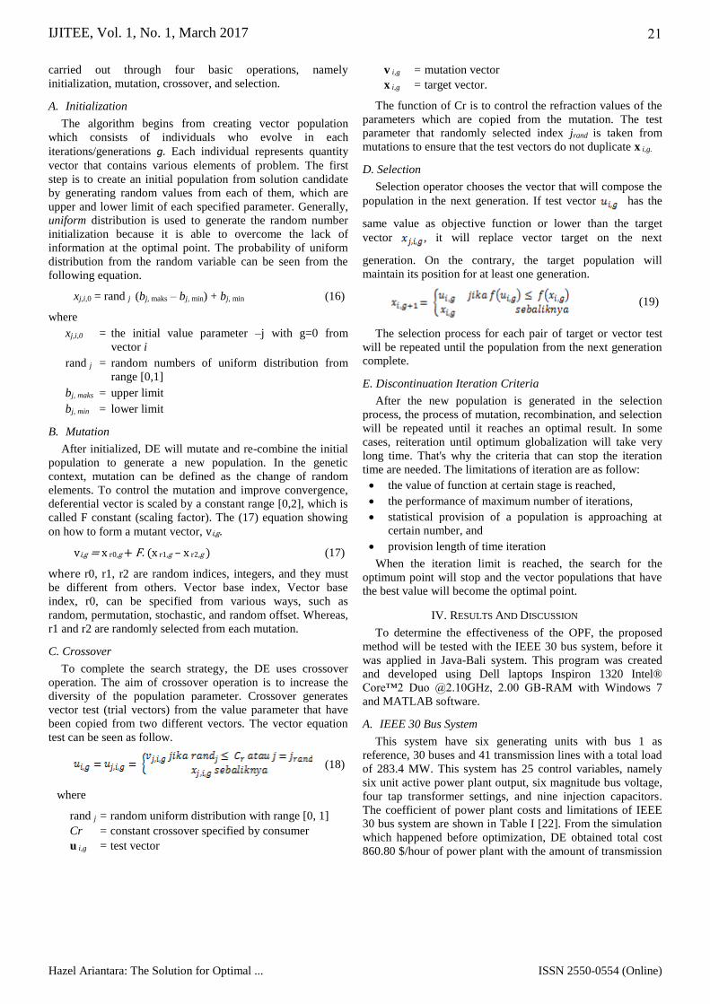
(1.05 pu), as shown in Fig. 2. Meanwhile, the power flow in

each channel was still within the operation boundaries with

the transmission line at the highest channel 91% on bus 1 to

bus 2. This is because the power plant at bus 1 (reference bus)

receive greater load than the other plant. The results of

imposition channel simulation are shown in Fig. 3.

Fig. 2 Voltage profile bus after optimization OPF-DE.

Fig. 3 Imposition channel after optimization OPF-DE.

TABLE III THE COMPARISON OF SIMULATED RESULTS IN IEEE 30 BUS SYSTEMS

Optimization

Method

Power Plant Cost

($/hour) Transmission Loss

DE 800.500 9.028

GA [17] 801.960 9.080

FGA [17] 801.121 9.030

PSO [17] 800.960 9.080

FPSO [17] 800.720 8.750

Bat Algorithm[23] 800.929 9.220

The comparison of simulation results in the DE with the

proposed methods such as GA method [17], fuzzy GA [17],

PSO [17], fuzzy PSO [17], and bat algorithm [23] can be seen

in Table III. The results show that the cost saving is

$0.22/hour compared to the FPSO and $0.429/hour compared

to the bat algorithm method. Based on Table III, it can be

concluded that the DE method is more reliable and could be

applied in real system.

B. 500 kV Java-Bali System

The Java-Bali 500 kV system used in this study refers to

two previous studies [23], [24]. This system consists of eight

stations, 25 buses and 30 transmission lines. Surayala power

plant unit is the reference bus while the Muaratawar, Cirata,

22



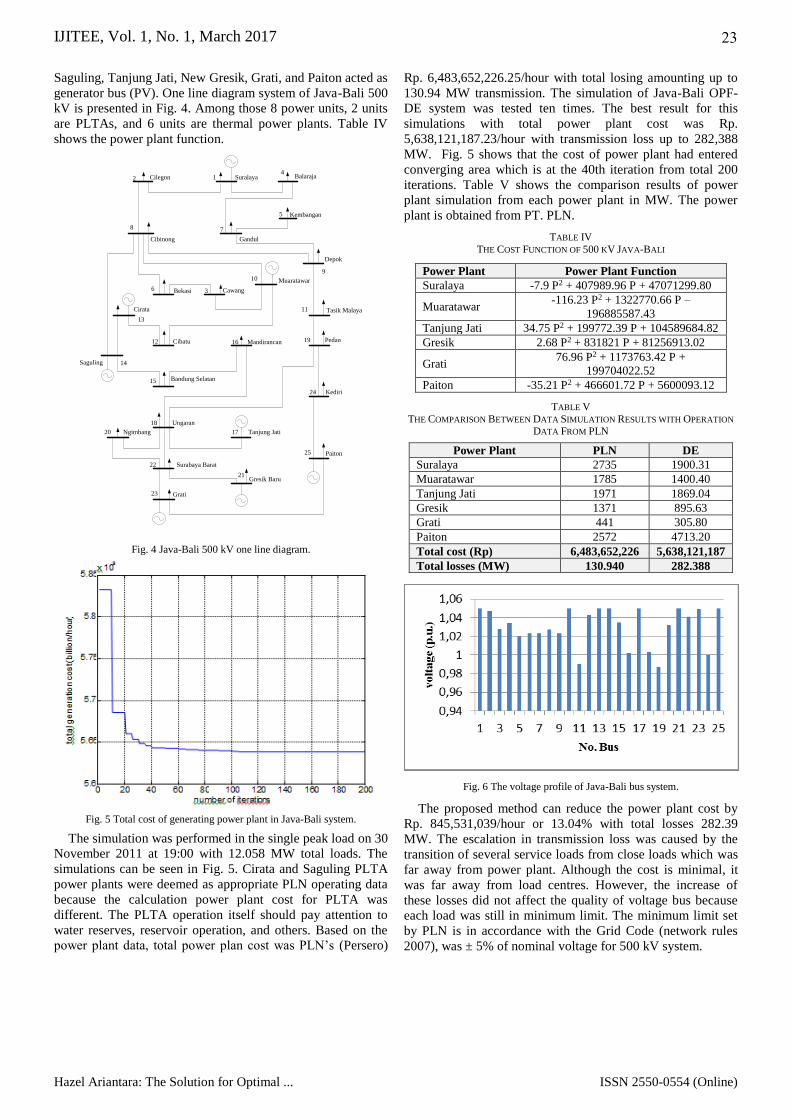
Saguling, Tanjung Jati, New Gresik, Grati, and Paiton acted as

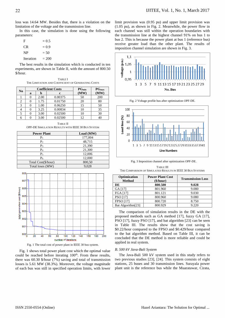
generator bus (PV). One line diagram system of Java-Bali 500

kV is presented in Fig. 4. Among those 8 power units, 2 units

are PLTAs, and 6 units are thermal power plants. Table IV

shows the power plant function.

Suralaya1Cilegon2

Cawang3

Balaraja4

Kembangan5

Bekasi6

Gandul

7

Cibinong

8

Depok

9

Muaratawar10

Tasik Malaya11

Cibatu

Cirata

12

13

Saguling 14

Bandung Selatan15

Mandirancan16

Tanjung Jati17

Ungaran18

Pedan19

Ngimbang20

Gresik Baru21

Surabaya Barat22

Grati23

Kediri24

Paiton25

Fig. 4 Java-Bali 500 kV one line diagram.

Fig. 5 Total cost of generating power plant in Java-Bali system.

The simulation was performed in the single peak load on 30

November 2011 at 19:00 with 12.058 MW total loads. The

simulations can be seen in Fig. 5. Cirata and Saguling PLTA

power plants were deemed as appropriate PLN operating data

because the calculation power plant cost for PLTA was

different. The PLTA operation itself should pay attention to

water reserves, reservoir operation, and others. Based on the

power plant data, total power plan cost was PLN’s (Persero)

Rp. 6,483,652,226.25/hour with total losing amounting up to

130.94 MW transmission. The simulation of Java-Bali OPF-

DE system was tested ten times. The best result for this

simulations with total power plant cost was Rp.

5,638,121,187.23/hour with transmission loss up to 282,388

MW. Fig. 5 shows that the cost of power plant had entered

converging area which is at the 40th iteration from total 200

iterations. Table V shows the comparison results of power

plant simulation from each power plant in MW. The power

plant is obtained from PT. PLN.

TABLE IV

THE COST FUNCTION OF 500 KV JAVA-BALI

Power Plant Power Plant Function

Suralaya -7.9 P2 + 407989.96 P + 47071299.80

Muaratawar -116.23 P2 + 1322770.66 P –

196885587.43

Tanjung Jati 34.75 P2 + 199772.39 P + 104589684.82

Gresik 2.68 P2 + 831821 P + 81256913.02

Grati 76.96 P2 + 1173763.42 P +

199704022.52

Paiton -35.21 P2 + 466601.72 P + 5600093.12

TABLE V

THE COMPARISON BETWEEN DATA SIMULATION RESULTS WITH OPERATION

DATA FROM PLN

Power Plant PLN DE

Suralaya 2735 1900.31

Muaratawar 1785 1400.40

Tanjung Jati 1971 1869.04

Gresik 1371 895.63

Grati 441 305.80

Paiton 2572 4713.20

Total cost (Rp) 6,483,652,226 5,638,121,187

Total losses (MW) 130.940 282.388

Fig. 6 The voltage profile of Java-Bali bus system.

The proposed method can reduce the power plant cost by

Rp. 845,531,039/hour or 13.04% with total losses 282.39

MW. The escalation in transmission loss was caused by the

transition of several service loads from close loads which was

far away from power plant. Although the cost is minimal, it

was far away from load centres. However, the increase of

these losses did not affect the quality of voltage bus because

each load was still in minimum limit. The minimum limit set

by PLN is in accordance with the Grid Code (network rules

2007), was ± 5% of nominal voltage for 500 kV system.

23



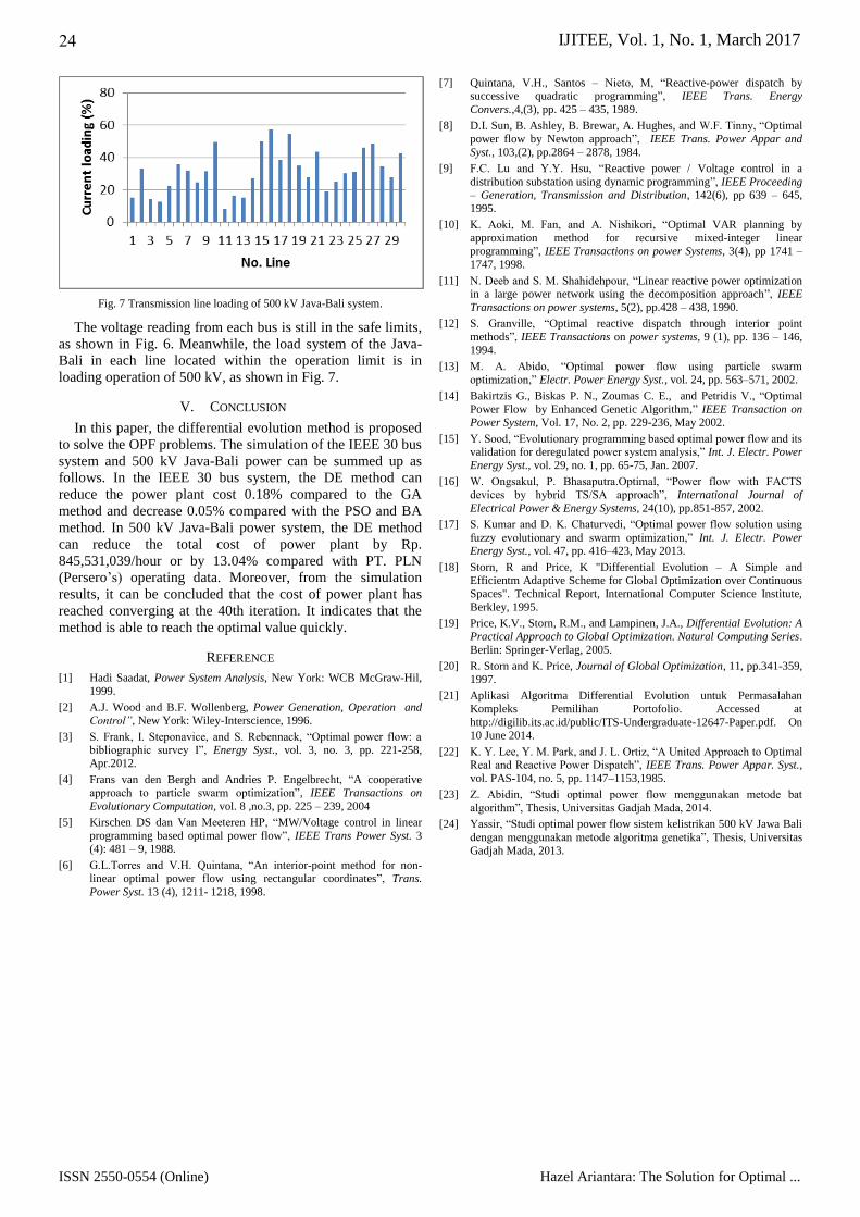
Fig. 7 Transmission line loading of 500 kV Java-Bali system.

The voltage reading from each bus is still in the safe limits,

as shown in Fig. 6. Meanwhile, the load system of the Java-

Bali in each line located within the operation limit is in

loading operation of 500 kV, as shown in Fig. 7.

V. CONCLUSION

In this paper, the differential evolution method is proposed

to solve the OPF problems. The simulation of the IEEE 30 bus

system and 500 kV Java-Bali power can be summed up as

follows. In the IEEE 30 bus system, the DE method can

reduce the power plant cost 0.18% compared to the GA

method and decrease 0.05% compared with the PSO and BA

method. In 500 kV Java-Bali power system, the DE method

can reduce the total cost of power plant by Rp.

845,531,039/hour or by 13.04% compared with PT. PLN

(Persero’s) operating data. Moreover, from the simulation

results, it can be concluded that the cost of power plant has

reached converging at the 40th iteration. It indicates that the

method is able to reach the optimal value quickly.

REFERENCE

[1] Hadi Saadat, Power System Analysis, New York: WCB McGraw-Hil,

1999.

[2] A.J. Wood and B.F. Wollenberg, Power Generation, Operation and Control”, New York: Wiley-Interscience, 1996.

[3] S. Frank, I. Steponavice, and S. Rebennack, “Optimal power flow: a bibliographic survey I”, Energy Syst., vol. 3, no. 3, pp. 221-258,

Apr.2012.

[4] Frans van den Bergh and Andries P. Engelbrecht, “A cooperative

approach to particle swarm optimization”, IEEE Transactions on

Evolutionary Computation, vol. 8 ,no.3, pp. 225 – 239, 2004

[5] Kirschen DS dan Van Meeteren HP, “MW/Voltage control in linear

programming based optimal power flow”, IEEE Trans Power Syst. 3 (4): 481 – 9, 1988.

[6] G.L.Torres and V.H. Quintana, “An interior-point method for non-linear optimal power flow using rectangular coordinates”, Trans.

Power Syst. 13 (4), 1211- 1218, 1998.

[7] Quintana, V.H., Santos – Nieto, M, “Reactive-power dispatch by successive quadratic programming”, IEEE Trans. Energy

Convers.,4,(3), pp. 425 – 435, 1989.

[8] D.I. Sun, B. Ashley, B. Brewar, A. Hughes, and W.F. Tinny, “Optimal

power flow by Newton approach”, IEEE Trans. Power Appar and

Syst., 103,(2), pp.2864 – 2878, 1984.

[9] F.C. Lu and Y.Y. Hsu, “Reactive power / Voltage control in a

distribution substation using dynamic programming”, IEEE Proceeding – Generation, Transmission and Distribution, 142(6), pp 639 – 645,

1995.

[10] K. Aoki, M. Fan, and A. Nishikori, “Optimal VAR planning by

approximation method for recursive mixed-integer linear

programming”, IEEE Transactions on power Systems, 3(4), pp 1741 – 1747, 1998.

[11] N. Deeb and S. M. Shahidehpour, “Linear reactive power optimization in a large power network using the decomposition approach”, IEEE

Transactions on power systems, 5(2), pp.428 – 438, 1990.

[12] S. Granville, “Optimal reactive dispatch through interior point

methods”, IEEE Transactions on power systems, 9 (1), pp. 136 – 146,

1994.

[13] M. A. Abido, “Optimal power flow using particle swarm

optimization,” Electr. Power Energy Syst., vol. 24, pp. 563–571, 2002.

[14] Bakirtzis G., Biskas P. N., Zoumas C. E., and Petridis V., “Optimal

Power Flow by Enhanced Genetic Algorithm,” IEEE Transaction on Power System, Vol. 17, No. 2, pp. 229-236, May 2002.

[15] Y. Sood, “Evolutionary programming based optimal power flow and its validation for deregulated power system analysis,” Int. J. Electr. Power

Energy Syst., vol. 29, no. 1, pp. 65-75, Jan. 2007.

[16] W. Ongsakul, P. Bhasaputra.Optimal, “Power flow with FACTS

devices by hybrid TS/SA approach”, International Journal of

Electrical Power & Energy Systems, 24(10), pp.851-857, 2002.

[17] S. Kumar and D. K. Chaturvedi, “Optimal power flow solution using

fuzzy evolutionary and swarm optimization,” Int. J. Electr. Power Energy Syst., vol. 47, pp. 416–423, May 2013.

[18] Storn, R and Price, K "Differential Evolution – A Simple and Efficientm Adaptive Scheme for Global Optimization over Continuous

Spaces". Technical Report, International Computer Science Institute,

Berkley, 1995.

[19] Price, K.V., Storn, R.M., and Lampinen, J.A., Differential Evolution: A Practical Approach to Global Optimization. Natural Computing Series.

Berlin: Springer-Verlag, 2005.

[20] R. Storn and K. Price, Journal of Global Optimization, 11, pp.341-359,

1997.

[21] Aplikasi Algoritma Differential Evolution untuk Permasalahan

Kompleks Pemilihan Portofolio. Accessed at

http://digilib.its.ac.id/public/ITS-Undergraduate-12647-Paper.pdf. On 10 June 2014.

[22] K. Y. Lee, Y. M. Park, and J. L. Ortiz, “A United Approach to Optimal Real and Reactive Power Dispatch”, IEEE Trans. Power Appar. Syst.,

vol. PAS-104, no. 5, pp. 1147–1153,1985.

[23] Z. Abidin, “Studi optimal power flow menggunakan metode bat

algorithm”, Thesis, Universitas Gadjah Mada, 2014.

[24] Yassir, “Studi optimal power flow sistem kelistrikan 500 kV Jawa Bali

dengan menggunakan metode algoritma genetika”, Thesis, Universitas

Gadjah Mada, 2013.

24

http://ieeexplore.ieee.org.ezproxy.ugm.ac.id/xpl/RecentIssue.jsp?punumber=4235

Documents

The Solution for Optimal Power Flow (OPF) Method Using