1. THE SPANWISE PERTURBATION O F TWO-DIMENSIONAL

BOUNDARY LAYERS

2. THE TURBULENT RAYLEIGH PROBLEM

3. THE PROPAGATION OF F R E E TURBULENCE IN

A MEAN SHEAR FLOW

Thes i s by

Steven Collins Crow

In P a r t i a l Fulfi l lment of the Requi rements

F o r the Degree of

Doctor of Philosophy

California Institute of Technology

Pasadena, California

1946

(Submitted M a y 2 7 , B 9 6 4 )

-ii-

ACKNOWLEDGMENTS

Pe te r Bradshaw and Trevor Stuart a t the National Physical

Laboratory in England suggested the boundary-layer problem solved

in the f i r s t chapter of this thesis , I began the work under their in-

spiration and continued with the guidance of Philip Saffman a t Caltech.

Pe te r Bradshawls des i re to incorporate the Townsend s t r e s s - shea r

relation in turbulent boundary-layer s imilari ty solutions led me to

develop the turbulent Rayleigh problem. Bradshaw' s enthusiasm

and his experiments motivated my work during my stay in England.

Philip Saffman suggested the problem of propagation of turbulence

through a mean shear flow. He helped me through initial difficulties

and made many suggestions which have been incorporated in the

thesis . He was always ready to talk about the essential ideas behind

the work, and he was a lso willing to help on troublesome mathemat-

ical details. I thank Pe t e r Bradshaw, Trevor Stuart , and especially

Philip Saffman for their encouragement and their contributions to my

resea rch ,

Elizabeth Fox worked a s hard typing the thesis a s I did writing

it , I thank he r for a beautiful job on a long and complicated project.

Finally, I thank the National Science Foundation for the Fe l -

lowship which made my graduate study possible,

-iii-

ABSTRACT

1. The Spanwise Perturbat ion of Two-Dimensional Boundary Layers

Large spanwise variations of boundary-layer thickness have

recently been found in wind tunnels designed to maintain two-dimen-

sional flow. Bradshaw argues that these variations a r e caused by

minute deflections of the f ree - s t ream flow ra ther than an intrinsic

boundary-layer instability. The effect of a small , periodic t rans - ve r se flow on a flat-plate boundary layer i s studied in this chapter.

The t ransverse flow i s found to produce spanwise thickness variations

whose amplitude increases l inearly with distance downstream.

2. The Turbulent Rayleigh Problem

Rayleigh flow i s the non- steady motion of fluid above a flat

plate accelerated suddenly into motion. Laminar RayPeigh flow i s

closely analogous to laminar boundary-layer flow but does not involve

the analytical difficulty of non-linear convection. In this chapter ,

turbulent Rayleigh flow i s studied to illuminate physical ideas used

recently in boundary-layer theory. Boundary Payers have nearly

s imilar profiles for certain r a t e s of p ressure change. The Wayleigh

problem i s shown to have a c lass of exactly s imi lar solutions.

Townsend's energy balance argument for the wall layer and Cliauser's

constant eddy viscosity assumption for the outer layer a r e adapted

to the Rayleigh problem to fix the relation between shear and s t r e s s ,

The resulting non-linear, ordinary differential equation of motion is

solved exactly for constant wall s t r e s s p analogous to ze ro p ressure

gradient in the boundary-layer problem, and for zero wall s t r e s s ,

anaIogous to continuously separating flow. Finally, the boundary -

- iv -

l a y e r equations a r e expanded in powers of the skin friction parameter

y = d v , and the zeroth order problem i s shown to be identical to

t h e Rayleigh problem. The turbulent Rayleigh problem i s not merely

a n analogy, but i s a rational approximation to the turbulent boundary-

l aye r problem.

3. The Propagation of F r e e Turbulence in a Mean Shear Flow

This chapter begins with the assumption that the propagation

of turbulence through a rapidly shearing flow depends pr imar i ly on

random stretching of mean vorticity. The Reynolds s t r e s s o (y , t )

acting on a mean flow U(y) = %2y in the x direction is computed from

the linearized equations of motion, Turbulence homogeneous in x , z

and concentrated near y = 0 was expected to catalyze the growth of

turbulence further out by stretching mean vorticity , but ~ ( y , t ) i s

found to become steady a s a t -" m. As f a r a s Reynolds s t r e s s i s a

measu re of turbulent intensity, random stretching of mean vorticity

alone cannot yield steadily propagating turbulence.

The problem i s simplified by assuming that a11 flow proper-

t i e s a r e independent of x, Eddy motion in the y, z plane i s then

independent of the x momentum i t t ranspor ts , and the mean speed

U(y, t ) i s diffused passively, The equations of motion a r e partially

linearized by neglecting convection of eddies in the y, z plane, and

wave equations for ~ ( y , t ) and U(y, t ) a r e derived, The solutions a r e

worthless , however, for l a rge times. Turbulence artificially steady

in the y, z plane forces the mean speed gradient steadily to zero , In

a rea l flow the eddies d isperse a s fas t a s U diffuses.

-v-

Numerical experiments a r e designed to find how quickly con-

centrated vortex columns parallel to x disperse over the y, z plane

and how effectively they diffuse U. It is shown that unless a lower

limit on the distance between any two vortices i s imposed, computa-

tional e r r o r s can dominate the solution no matter how small a time

increment i s used. Vortices which approach closely must be united.

Uniting vortices during the computations i s justified by finding a

capture c ros s section for two vortices interacting in a s t ra in field,

The experiments confirm the result that columnar eddies disperse

a s fast a s they transport momentum.

TABLEOF CONTENTS

PART TITLE PAGE

I. TI-IE SPANWISE PERTURBATION OF TWO- DIMENSIONAL BOUNDARY LAYERS

1 . Introduction

2. Statement of the Problem

3. Solution F a r Upstream

4. Outer Expansion

5. Inner Expans ion

4 . Matching

7. Initial Steps in Solving the Problem

8. Final Steps to Determine F 2

9. Conclusion

REFERENCES

11 . THE TURBULENT RAYLEIGH PROBLEM

1. Introduction

2. Similarity Fo rm of the Rayleigh Problem

for Self -Preserving Solutions

3. Some Proper t ies of the Self -Preserving Solutions

A. Momentum Conservation

B, Laminar Sublayer

4. Assumptions for the a(a) Relation

A. Wall Eayer

Be Outer Layer

5. Equations of Motion under the ~ ( o ) Assump-

tions - Some General Consequences

-vii-

TABLE OF CONTENTS (Cont'd)

PART TITLE PACE

6. Solution for the Constant S t ress Case , c = 0 4 2

7, Solution for the Continuously Separating

Case , c = -1 44

8. Analogy with the Equilibrium Boundary Layer 50

REFERENCES 66

APPENDIX 67

111, THEPROPAGATIONOFFREETURBULENCE

IN A MEAN SHEAR FLOW 7 1

1. Introduction 7 1

2. Basic Equations of the Problem 77

3. The Linearized Problem with Constant SE 83

A. Four ie r Transformation and Solution

of the Linearized Equations of Motion 8 3

B, Correlation and Spectrum Functions of

the Solutions to the Linear Problem 89

C. Reynolds S t ress above a Sheet of Random

Vorticity 92

D. Reynolds S t ress in the Limit SEt " co

of the General Problem 102

4, Flow Uniform in the x Direction 106

A. The i 3~ /8x = 0 Assumption 106

Be The Random Vortex Sheet Problem

with B F / B X = 8

C, Steady Kduction by Line Vortices of

TABLE O F CONTENTS (Cont'd)

PART TITLE

Alternating Sign

5. The Numerical Experiments

A, Basis of the Numerical Approach

Be Generation of Random Vortex Strengths

a Specified Correlation

C , E r r o r Ilrift i

D, Flow Velocity and E r r o r Velocity

E. Vortex Capture 5

E . Flow Visualization Experiments

G. Background for the Momentum Trans fe r

Experiments

H. Momentum Transfer Experiments

6. Summary

REFERENCES

APPENDICES

A. Evaluation of L.. (_k. ko2) XJ

B. Evaluation of the S t r e s s Integrals in

the Vortex Sheet Problem

C, Proof that Equation 31 i s Valid in the

Limit S;Et co

D. Singular Perturbat ion Solution for

s(q9.19 .(q 9 .I

E, Derivation of T($) and +(yp 0) for the

PAGE

129

136

136

Steady Vortex Street

TABLE OF CONTENTS (Cont'd)

PART TITLE PAGE

F. Derivation of the Mean Square E r r o r - Velocity

2 E C

C. Motion of the Center of a Continuous

Vorticity Distribution in a Uniform

Translation and Strain Field

- 1 - I . THE SPANWISE PERTURBATION OF TWO -DIMENSIONAL

BOUNDARY LAYERS

1. Introduction

In a s e r i e s of wind-tunnel t e s t s under nominally two-dimen-

sional conditions, Klebanoff and Tids t rom [ 1 I/ found quasi-periodic

spanwise variat ions of boundary-layer thickness of o r d e r * 8%.

Recently the phenomenon r e c u r r e d in a National Physical Laboratory

tunnel specifically designed for the study of two -dimensional boundary

l aye r s . Bradshaw [ Z ] sought a remedy a s well a s a n explanation and

found that these variat ions could resu l t f rom la t e ra l convergence o r

divergence of the flow downstream of slightly non-uniform sett l ing-

chamber damping sc reens . A rough analysis suggested that a bound-

a r y layer i s surpris ingly sensit ive to spanwise velocity var iat ions.

The thickness var iat ions found by Klebanoff could have been produced

by variat ions in the f r e e - s t r e a m flow direction of around 0.04 de-

g r e e , much too sma l l t~ be measured direct ly . This chapter i s a

r igorous analysis of the effect of a sma l l , periodic spanwise com-

ponent of velocity on the boundary layer of a flat plate. The flow i s

assumed to be incompressible , steady and l amina r .

Three-dimensional effects in the boundary layer will depend

on the t r ansve r se flow field chosen fo r the incident flow. Suppose

U charac ter izes the chordwise component of f r e e - s t r e a m flow, 0

yU the amplitude of the t r ansve r se perturbation. Suppose the f r e - 0

quency of the spanwise flow is specified by a wave-number k. The

Reynolds number of the perturbation is then

R = =yu0/kv

- 2 -

If Bradshaw's explanation i s co r rec t , the value of R corresponding to

Klebanoff's data can be computed, and it i s found to be around 3 . It

i s not surprising that R i s of o rder 1, since the t r ansverse velocity

variations a r e supposed to a r i s e from the non-uniform drag of damp-

ing screens-a viscous phenomenon to begin with. R will be regarded

a s a parameter of order 1 throughout the analysis .

2. Statement of the Problem

The momentum and continuity equations a r e

for a steady, incompressible flow field = ( U , V , W ) . The coordi-

nates and physical situation a r e shown in figure 1. F o r a character -

istic speed Ug and perturbation wave-number k, the following

non-dimensional variables a r e appropriate:

The equations of motion in non-dimensional form a re :

2 (6-momentum) uu + vu + wui = -p6 + E (uE5 4- uqq + U 5 5 ) $ 5

2 5 'pl 5

- -pq t r (V (q-momentum) uv + vv + wv - 2

55 ' v7a7a ' "55) (<-momentum) uw 8- vw -I- WW - 5 "'1

5- -pgf E (w ~ 5 * ~ r l r l + ~ 5 5 ) #

(continuity) u + v t w = 0 9 5 7 5

-4-

where e 2 = vk/u0. If y i s the amplitude of the angular variation of

f ree -s t ream flow direction, the perturbation Reynolds number i s

R = y ~ o / k v = y / r 2 - o(I.).

In Klebanoff' s experiments y was typically 0. 40° - 0.001 rad. , so E

was about 0.02. In this chapter E i s used a s an expansion parameter

i n a perturbation scheme.

The boundary condition a t the plate i s

The upstream flow can be specified in any convenient way a s long a s

the field chosen ca r r i e s the desired t ransverse perturbation and is

a n adequate approximation to a solution of the equations of motion.

Le t the expansions for u and w in the outer flow begin

u = l + ..., 2

W = y cos < + ... = R E c s s 5 + ...,

3 . Solution F a r Upstream

The velocity components above cannot be worked into a uni-

formly convergent solution to the equations of motion. Since the

Reynolds number of the perturbation i s of order I , the transverse

field of the incident s tream mustdecay under the action of viscosity.

Suppose we t ry a soPutisn of the form

2 w = R ( ~ ) E cos 5,

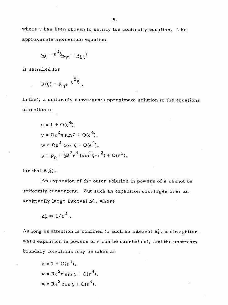
- 5 -

where v has been chosen to satisfy the continuity equation. The

approximate momentum equation

i s satisfied for

In fact, a uniformly convergent approximate solution to the equations

of motion i s

4 u = a. + O(E ),

2 4 v = RE q s i n g + O(E 1,

2 4 w = R E cos 5 f O(E ),

2 4 2 2 4 p = p + $R E (s in 5-q ) + O(E ) 9 0

for that R ( 5 ) .

An expansion of the outer solution in powers of E cannot be

uniformly convergent. But such an expansion converges over an

arbi t rar i ly large interval A $ , where

As long a s attention i s confined to such a n interval 8 5 , a straightfor-

ward expansion in powers of E can be ca r r i ed out, and the upstream

boundary conditions may be taken a s

-6 -

4 where change in R i s now contained in the O(E ) corrections.

4. Outer Expansion

Let c y y, 5 remain fixed, and allow E to tend to zero. The

dependent variables a r e expanded in powers of E a s follows:

When the coefficients of consecutive powers of E in the equations of

motion a r e se t equal to zero, the following system of equations

results:

5 momentum

q momentum

Q ( 4 gI5 = -pIq2

2 - O(E ) f1815 + 82% + gigll - -P2?.

t: momentum

Q ( t ) PIC = 0 ,

2 O(E 1 PZG = 0 .

Continuity

o(t) f i e + g l q = 09

2 O(c f2e +- gzq - R s i n g = 0.

No boundary conditions a r e available a t the plate. The outer

expansion must be matched to an inner (boundary-layer) expansion

there. In accordance with the discussion of the previous section, the

conditions far upstream a r e f l , f2,fg9gl + 0. ' F a r upstream' means

-$>> I ; we cannot really permit -5 " oo, since the expansion form

- 2 assumed i s valid only in an interval AS CC E .

5. Inner Expansion C

An expanded boundary-layer variable q = q / ~ must be used to

bring out the behaviour of the fluid near the plate. Then let 5 , ;, 5

remain fixed, and allow 6 to approach zero. The dependent variables

a r e again expanded in powers of E:

The equations of motion split up into the following system:

5 momentum

O(1) FOFOg f GIFO; = -- or17

( 9 )

O ( E ) F F +IFF - ! - G I ? - + G I ? - = - P t F - - , (10) 1 sg o 16 2 0q 1 Br( 15 1T-l

+ HzFog = - P25fF055+F2:;f FOG5* (11)

q momentum

5. momentum

Continuity

At the plate al l t e rms in the expansions of up V , w a r e zero.

Fur ther conditions a r e provided by matching the inner and outer so-

lutions in an intermediate region where they a r e simultaneously valid.

6 , Matching

The forms assumed for the inner and outer expansions a r e

valid only i f the solutions based on them can be matched. Since

matching must be done step-by- step in the analysis which folPows,

general equations for the procedure a r e derived here.

Consider the inner and outer expansions of any dependent

variable a:

The matching is done on an intermediate variable q* = ~ / x ( E ) such

that, for q:: fixed and E + 0,

The outer solution may be expanded around q = 0 in the form

where the arguments of each function on the right a r e ( 5 , 0,g). The

inner solution has the form

In order for the two expansions to match for q * fixed and E - 0, the

following conditions must hold:

7. Initial Steps in Solving the Problem

The solution must be carr ied to second order in E to show the

most interesting effects produced by the t ransverse field of the inci-

dent flow. The program can be carr ied out by finding solutions to a

sequence of groups of the equations (1 )-(I 8). The functions Fo, F1,

G1 G2, H2' f1 f Z 9 g1 g2 a r e found that way in the five steps of this

section. That i s preliminary. The effect s f the t ransverse field on

the chordwise flow i s uncovered only when F is found, and that i s 2

deferred to $8.

At the beginning of each of the steps below the ingredients

needed a r e listed-the equations from the system (6)-(3181, the bomnd-

a ry conditions, and the matching conditions .

F i r s t step-determining F and GI 0

equations: (9 )s (16)

boundary conditions: FO($, 0 ,5) = 0, (a)

G1 ( $ t o , 5 ) = 0, (b)

matching condition: F0(5, m, 5) = 1 . (c )

Let Fo = *-+. Then equation (16) becomes '1

Hence GI = -Y5 f fn(5 ,5) ,

where fn(Cs 5 ) i s zero i d (b) i s satisfied by putting 9 (5, 0, 5 ) = 0. 5 Equation (9) becomes

Then Q(s ) satisfies

Fo and Gl become

so conditions (a) , (bIp ( c ) a r e

J ( s ) i s thus the Blasius function. Suppose P i s defined a s follows:

Then

Notice Fg and C$ do not depend on 5.

Second step-determining H2

equations : (5). ( 6 ) s (1319 (15)

boundary condition: H2(S9 0.5) = 0, (a)

matching conditions: H2(ey m y 5) = Rcosc, (b)

The matching conditions here , a s elsewhere, a r e applications of the

general matching equations derived ear l ier . (c) , fpr example, i s

the second-order matching condition for p with p ' = 0. Equation 0rl'l

(13) may be written

Since F and GI do not depend on 5, P - - 0 - 4 5 - 0, so P

25 = fn(g95). Dif-

ferentiating ( c ) on 5 and using equations (5) and (6) yield lim PZ5= 0. ?-

Thus

everywhere. Equation (15) then becomes

which is the same a s equation (9) i f Hz = f n ( ~ ) ~ ~ ( 6 ~ < ) . The solution

-12 -

satisfying conditions (a) and (b) i s

Thus the spanwise flow follows the Blasius profile to the o rder con-

sidered.

Third step-determining fl , gl and pl

equations: (11, (31, (5)s (7)

boundary conditions: f19 gl-' 0 f a r ups t ream, (a)

matching condition: Gl(L = g l (L O , G ) . (b)

Equations (1 ) and ( 3 ) , flS = -pie and gle = -plq9 combine to

give t h e equation for conservation of spanwise vorticity ,

By the upstream conditions (a),

Equations (1 ), (3) and (5) then imply

Since the spanwise vorticity i s zero , there i s a potential function 4

such that

f 1 = 4 5 s g 1 = O q 9

and equation ('9) becomes

Condition (b) and the expression for G1(c,m) found in the f i r s t s tep

give

over the plate. is thus the linearized. potential for flow around a

thin parabolic cylinder (van Dyke [ 3 ] ). The solution sat isf ies

next to the plate, and f and g do not depend on 5. 1 1

Fourth step-determining F and G2 l

equations: (101, ( 1 2 ) ~ ( l4 ) t (17)

boundary conditions: FIE$ 0 . 5 ) = 0, (a )

c2(6, 0, 5 ) = 0, (b)

matching conditions: F l ( $ d % f ) = f l ( 5 d a = 0, (c)

p , ( 6 , o o , 5 ) = ~ ~ ( 5 . 0 ) = ~ . (dl

Since equations (12) and (14) imply PI = Pl(5) , condition (d) requires

P = 0. Equations (10) and (17) a r e thus homogeneous and l inear in 1

F and G2, and the only solution compatible with conditions (a) , (b) 1

and ( c ) i s

Fp = G2 = 0.

Fifth step-determining f 2 , g2 and p2

equations: (2Ip (4), (6 )9 ( a ) 9 68)

boundary condition: f2 -0 f a r upstream, (a ) IV

matching condition: qglq (c, O)+g2(e, 0 , G ) = l im G2 = 0. (b) : +m

- 14 - By equation (7) g = -f15, and f rom the third s tep f ( 5 , O ) = 0.

1 rl 1

Hence

and (b) becomes

In the third step it was shown that f - 17 - g1.$9 so equations (2), (4),

(6) and (8) can be written

and the solution satisfying conditions (a) and (b) i s

8. Final Steps to Determine Fz

In the l a s t section it was shown that the f i r s t -o rder correction

to the chordwise boundary-layer profile i s zero. If the theory i s going

to account for the large boundary-layer Fhickness and shear variations

observed by Klebansff and Bradshaw, those effects will have to show

up in the function F2 yet to be calculated. The trouble i s that even in

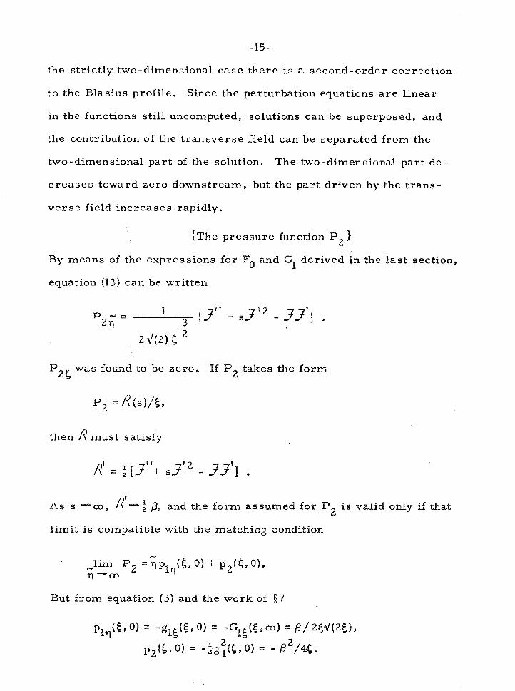
the strictly two-dimensional case there i s a second-order correction

to the Blasius profile. Since the perturbation equations a r e linear

in the functions still uncomputed, solutions can be superposed, and

the contribution of the t ransverse field can be separated from the

two-dimensional part of the solution. The two-dimensional part de - creases toward zero downstream, but the part driven by the t rans -

ve r se field increases rapidly.

he pressure function P } 2

By means of the expressions for lFg and % derived in the l as t section,

equation (13) can be written

P was found to be zero. Pf P2 takes the form 2 5

P2 = fi(s)/E,

then 8 must satisfy

As s +mx,, f l t - ~ /3$ and the form assumed fox P i s valid only if that 2

limit i s compatible with the matching condition

But from equation ( 3 ) and the work of $7

Hence

-1im p2 = /3s/25 - p2/45, rl -a

which i s compatible with the form assumed ea r l i e r if the constant of

integration for 8 i s chosen such that

ransf sf or mat ion of the equation for F } 2

Since F1 = G2 = F = 0 and H2 = RFOcos 5, equations (11) and (18) a r e 05

Le t Fo = %fN a s before, and le t F = x;. Then the continuity equation '1 2

becomes

- 4 - G - = R s i n G 9 ; . . '&-I 31

Hence

and fn(5.5) = O i f the boundary condition G3(5. 0.5) = O is satisfied by

requiring x ($,O, 5) = 0. Now transform 5

in the momentum equation. Thus

'-d

>((5$q95) = X(Ess95) P

-17-

and Fo, G and P a r e already known in t e r m s of the new variables. 1 2

The equation becomes

x S s S + 3x Ss - 2 5 . 3 ' ~ ~ ~ t re3"xg + 3 'x s

The boundary conditions a t the plate a r e

The matching condition for F i s 2

From the l a s t section f 2 = 0 and fll(g, 0) = g15(5. 0) = - @/264(2g).

Hence

IU l im F2 = - @ s / 2 t 9

1-00

and

Iim XscE. s . i) = - / 3 ~ / d ( 2 5 ) ~ S -a

It i s easy to show by direct substitution that that l imit i s compatible

with the t ransformed momentum equation,

(separation of X into two- and three-dimensional parts)

In the t ransformed momentum equation there i s one t e rm which i s

-18 -

modulated by R sin 5 ; there a r e no such t e r m s in the boundary condi-

tions. That t e rm reflects the R sin &$ par t of G3 and i s a forcing

function imposed by the t r ansverse field through the continuity con-

dition, X can be written a s a sum of two par t s , one proportional to

R sin 5 and the other not involving & a t all. The f i r s t t e r m responds

to the forcing function proportional to R s in 5 and obeys ze ro boundary

conditions al l around. The second t e r m respons to the two-dimen-

sional forcing function and satisfies the Xs l imit for s + m . Thus

wri te

N ( s ) and /n ( s l a r e defined by separate differential equations and

boundary conditions:

If the spanwise vorticity i s to decay exponentially f a r from

the plate, N ( s ) must contain an O(log a ) t e rm (Van Dyke [ 3 ] ) . There

i s no need to find out more about N ( s ) . The important point i s that

the two-dimensional contribution % approaches zero a s 5 becomes

3/2 la rge , and the three-dimensional t e rm grows a s

-19 - {F2 and the boundary-layer profile }

The N equation with i t s boundary conditions has a s imple solution -

That can be verified by direct substitution using the Blasius equation

and i ts derivative. Then

The boundary-layer profile i s

1 1

u = -.?'(s) - f ~ E ' 5 s i n S s J ( s f t E2(/h'(s)/2$) t 0 ( c 3 ) .

Notice the expgnsion i s not uniformly convergent. The second t e rm

2 i s much smal ler than the f i r s t only i f 6 P/E , but that i s assured

L by the restr ict ion AE << I/E alrgady imposed to make the outer flow

2 tractable. The third t e rm i s small if f >> E , the usual requirement

f o r convergence of the boundary-layer expansion.

The f i r s t two t e r m s of the profile expansion can be combined

into a single function

with third-order accuracy. Then

where

2 and y = R a . Thus the shape of the profile i s unaffected by the t rans - v e r s e field. Even in the second-order approximation, the only three-

dimensional effect i s a spanwise variation in boundaey-layer

thic kne s s .

9. Conclusion

F o r the profile expansion to be valid, 5 must satisfy

2 a << 5 << l / a . In physical variables the inequality can be written

and in that interval, expressions good to O(y) fo r U and W a r e

where

(1 + *ykx sin kz).

Thus the boundary layer takes on the wavy character i l lustrated in

figure l. The practical significance of these resul ts i s discussed by

Bradshaw [2] .

-21-

REFERENCES

1. Klebanoff, P. S. and T ids t rom, K. D . , "Evolution of Amplified

Waves Leading to Transi t ion in a Boundary Layer with Z e r o

P r e s s u r e Gradient ," NASA TN D 195 (1959).

2 . Bradshaw, P. , "The Effect of Wind Tunnel Screens on Nominally

Two-Dimensional Boundary L a y e r s , " Journa l of Fluid

Mechanics, Vol. 22 (1965), pp. 679-688.

3 . Van Dyke, M. , Per turba t ion Methods in F lu id Mechanics, New

York, Academic P r e s s (1964), pp. 121-147.

-22 -

11. THE TURBULENT RAYLEIGH PROBLEM

1. Introduction

The essent ia l physical problem of turbulent shea r flow - to

find the relationship between mean flow distribution and turbulent

s t ruc ture - i s s t i l l unsolved. F o r the t ime being, a d hoc physical

hypotheses m u s t be injected into any theory of turbulent shea r flow,

and the best a theoret ic ian can do is inject a t the l eas t sensi t ive point

in the s t ruc tu re of a problem. F o r example, suppose we descr ibe

proper t ies of a boundary layer above a wall in a coordinate system

( x , y p z ) where x points downstream and y is perpendicular to the

wall. Le t ( U , V , 0 ) be the corresponding mean velocity components

and (u, v , w) be turbulent fluctuations f rom the mean. The boundary-

layer momentum equation is

where d ~ / d x is the mean p r e s s u r e gradient and o i s the kinematic

shea r s t r e s s (Townsend El] ). The full express ion f o r the s t r e s s is

but in the fully turbulent region the viscous t e r m is negligible. In

t e r m s of o and the mean velocity gradient

a quantity with the dimensions of viscosi ty can be defined a s

- 2 3 -

Then the calculated mean velocity profile U(y) i s fair ly insensitive to

assumptions made about the "eddy viscosity. "

The Prandt l mixing length theory, which gave

in the region of a boundary layer near the wall, amounted to li t t le

more than a plausible assumption on the eddy viscosity. But the re la -

tion above can be derived without the mixing length hypothesis by

making certain assumptions about the turbulent energy equation. At

the same time i t becomes evident where the original Prandt l relation

will break down. By balancing turbulent energy generation, turbulent

diffusion and dissipation, and by making certain s imilari ty a s sump-

tions for the wall l ayer , Townsend [ 2 ] shows that

where the t e rm with the coefficient B represents the effect of tarbu-

lent diffusion. The derivation of that equation and the assumptions

involved will be discussed l a te r in connection with the turbulent

RayPeigh problem. The important thing for now i s the form of the

relation: %2 i s a functional of the s t r e s s distribution. That will be

t rue of any velocity gradient -s t ress relation derived from energy

considerations. If equation 3 i s combined a s i t stands with the

equation of motion, an integro-differential equation i s the result .

Equation 3 may be regarded a s an ordinary f i r s t -o rder differential

equation for and solved:

When that i s inserted in equation 1 , an integral t e rm remains. Al-

ternately the momentum equation can be differentiated with respect

to y , and with the aid of the continuity relation

it may be rewritten in t e r m s of S1 and o:

But U and V must s t i l l be expressed a s integrals of 62.

The Rayleigh problem of shear flow involves none of the

purely kinematic difficulties of the boundary -layer problem, yet

the same physical ideas apply. In this problem the non-steady flow

above an infinite plate moving in the x-direction in the x-z plane i s

examined; the independent variables a r e y and t. The situation is

sketched in figure 1. The mean flow continuity equation i s automat-

ically satisfied, since V = 0 and the problem i s statistically homo-

geneous in x. The momentum equation i s

a form closely analogous to equation 4. The turbulent Rayleigh

problem i s discussed in detail in this chapter.

-26-

In 1956, Clauser [ 3 ] suggested that approximately s imi lar

solutions could be obtained for ' equilibrium" turbulent boundary

l aye r s , those for which the parameter

remains constant. 6'k i s a measure of the boundary-layer thickness,

o i s the wall s t r e s s , so /3 i s the rat io of p ressure force ac ro s s the W

boundary layer to shear force. But a skin friction parameter

a lso enters the boundary -layer momentum equation and prevents

exact s imilari ty (or "self-preservation, " cf. Townsend [ I , 21 ).

Since y has only a small effect on the resu l t s , useful quasi-similar

solutions can be obtained, and that program was recently ca r r i ed

out by Mellor and Gibson [4A, B ] . One of the simplifications of the

Rayleigh problem i s that exactly self-preserving solutions a r e pos-

sible. It i s that family of exactly s imi lar solutions which i s t reated

he re .

Rayleigh proposed his non-steady shear flow situation a s an

analog to the laminar boundary Payer, The convective t e r m s on the

left hand side of equation 1 can be written

where UT i s the mean flow speed and s is a streamline coordinate.

If this t e rm i s approximated by

then t and X/U, play analogous par ts in the non-steady and steady

problems. Since a turbulent boundary layer i s much fuller than a

laminar boundary l ayer , the velocities a t corresponding points being

more nearly equal to the f ree - s t ream velocity in the turbulent case ,

it might be conjectured that a Rayleigh type analogy would be more

significant for the turbulent layers . In fact i t i s found that i f the

equation of motion for the equilibrium boundary layer i s written in

similarity form and expanded in powers of y, the zeroth-order t e rm

i s the s imilari ty equation for the Rayleigh problem. Thus the Ray-

leigh problem contains al l the essential features of the boundary-

layer problem except for non- s imilari ty.

The plan of this chapter i s then a s follows: in order to find

the self-preserving sollutians, the RayBeigh problem i s put in s imi-

lar i ty fo rm, and some general. consequences of that form a r e d is -

cussed; the physical ideas used by Clauser , Townsend and lately by

Mellor and Gibson a r e cas t into a form suitable for the Rayleigh

problem; exact solutions for the constant wall s t r e s s and zero wall

s t r e s s cases a r e derived under the physical assumptions, and

propert ies of other solutions a r e discussed; the analogy between

the turbulent boundary layer and the Rayleigh situation i s developed.

The o- %2 forms s f the equations of motion, equations 4 and 6 , will

be used so Townsend's velocity gradient- s t r e s s relation can be used

when the time comes. That means that shear s t r e s s will be specified

a t the moving wall ra ther than the wall speed. Then the s t r e s s

distribution for the Rayleigh flow can be found without explicitly

including any assumptions about the laminar sublayer - that i s not

s tr ict ly possible for the boundary layer.

2 . Similarity Form of the Rayleigh Problem for Self - Pr eserving

Solutions

The problem f i r s t will be restated. The equation of motion

i s

and in order to solve a practical problem a relation ~ { a ) will have

to be found. The boundary and initial conditions a r e

If exactly similar solutions exist, o and $2 must have the forms

where I q =JL 9

I

l o i and 1 and o a r e functions of time only. The boundary condition a t

0

the wall must be compatible with the similari ty solutions,

ow(t) = const. oo(t)

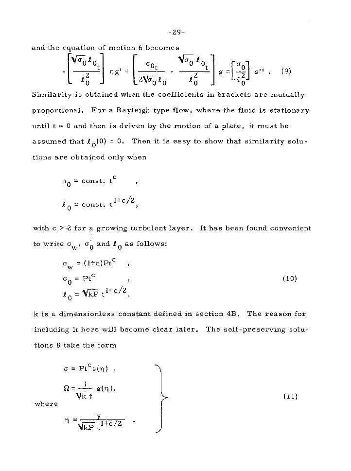
and the equation of motion 6 becomes

Similarity i s obtained when the coefficients in brackets a r e mutually

proportional. F o r a Rayleigh type flow, where the fluid i s stationary

until t = 0 and then i s driven by the motion of a plate, i t must be

assumed that 1 0(0) = 0. Then it i s easy to show that s imilari ty solu-

tions a r e obtaj;ned only when

C o0 = const. t s

with c >-2 for a growing turbulent layer. It has been found convenient

to write a o0 and l a s follows: w9

k i s a dirniensionless constant defined in section 4B. The reason for

including it he r e will become clear la ter . The self-preserving solu-

tions 8 take the form

B - g(rl)9

where

Equation 9 becomes

and conditions 7 reduce to

The condition c > - 2 insures that the turbulent layer grows, a s

it must for Rayleigh flow. The condition i s more res t r ic t ive than i s

necessary in the analogous boundary -layer c a se , since boundary lay-

e r s may actually contract under highly favorable p ressure gradients.

The case c = -1 corresponds to continuously separating flow with

zero wall s t r e s s . The cases -1 > c > - 2 involve various degrees of

separation and negative s t r e s s e s , and they a r e not discussed further .

I t i s assumed throughout that a l l s t r e s s e s a r e posit2ve to avoid cum-

bersome absoJute value signs.

3. Some Proper t ies of the Self -Preserving Solutions

A. Momentum Conservation

The equation for conservation of total momentum i s

a3

S w l t c U(y, t ) dy = - o ( t ' ) dt ' = -P t (14)

0 8

The Past equality follows from equation 18 except in the case c = - 1,

f o r then aw = 0. But in that case we assume that an amount of mo-

mentum L = -P has been injected into the field pr ior to t = 0. The

velocity a t any point in the field can be found f rom the momentum

equation. F r o m equations 5 and 11,

dt' ,

where

l t c r = - c '

lit- 2

and the l a s t of equations 11 h a s been used to find t s (y, q ' ) .

Since U has been expressed in t e r m s of s through the equation co I+@

of motion, i t i s obvious that S Udy m u s t equal - P t automatically 0

except perhaps in the c a s e c = - 1. Ee is interest ing to demonstrate

that explicitly though. By equations li 1 and 15,

The o r d e r of integration can be r e v e r s e d and the in tegra l evaluated

explicitly:

The f i r s t of equations 13 was used. The proof holds a s c approaches

- 1 but fa i l s f o r c = - 1. Going back to equation 15 for that c a s e ,

and in o r d e r that L = -P, s mus t sat isfy

It may seem strange that in this special c a s e an ex t r a condition like

equation 17 is imposed on the s t r e s s distribution s . But equation 12

f o r the c = - 1 c a s e with the boundary conditions s(O) = s ( m ) = 0 gives

a non-unique r e su l t , and equation 17 r emoves the non-uniqueness.

The physical reason why a n integral momentum condition is needed

f o r the continuously separating c a s e is c lear : in eve ry other c a s e

the momentum in the field i s determined by the h is tory of the s t r e s s

a t the wall , but in that c a s e the wall s t r e s s is ze ro and the momentum

i s injected into the field by unspecified means .

I3. Laminar Sublayer

An important taci t assumption h a s been made up to this point

which will now be justified. Immediately adjacent to the wall the flow

mus t be l a m i n a r , and the self -preserving solutions cannot be ex-

pected to hold in the laminar sublayer. The sublayer will extend to

some height hi and the s t r e s s will undergo some change Ao through v

it. Corresponding to b V , t he re will be some non-dimensional thick-

ness qv on the s imi lar i ty sca le , and the s imi lar i ty solutions of equa-

tion 12 will be valid only when

These two requirements a r e discussed below.

(i) The laminar sublayer becomes unstable a t a cr i t ica l Rey-

nolds number given by

(Clauser [ 3 ] ). The corresponding similari ty thickness q i s

where R i s the Reynolds number based on momentum in the field,

(ii) Suppose o = o + ay to a n adequate approximation in the W

laminas sublayer = Then

ao - ars - - a = - - ay at

and since a i s constant and atJ/at = eW a t the wall, where Cw i s the

acceleration of the wall,

Uw can be related to aw through a friction coefficient:

By using that expression to find 6 equations 10 for ow, and the ws

-34-

expression for L, it i s easily shown that

Except in the separating flow case , where the laminar sub-

layer does not have to t ransmit a mean s t r e s s boundary condition

anyway and i s generally supposed to be irrelevant , both q and

~ o / o go to ze ro a s R + co. The constant k , discussed in the next W

section, i s known to be about .015. and Cf could be about .003 for

a smooth plate under a wide range of Reynolds numbers. Then

conditions (i) and (ii) become

4. Assumptions for the Q(o) Relation

The reason for doing the Rayleigh problem i s that i t illumi-

nates the ideas used in boundary-layer theory more clearly than the

boundary-layer problem does. The purpose he r e i s not to introduce

new physical assumptions, but to adapt the ones ordinarily used to

the Rayleigh problem. The two-layer model of Clauses and Town-

send will be used, with a wall layer in energy equilibrium and an

outer layer of constant eddy viscosity, The object i s to find an ex-

pression for Q a s a functional of o reasonably well founded on physi-

ca l arguments. It muse be emphasized that the work up to now holds

independently of any assumptions about the relation Q(o) except that

i t be compatible with the s imilari ty form of the equations of motion.

The wall layer and outer layer will be treated separately.

A. Wall Layer

Townsend' s energy equilibrium argument [ 2 1 can be taken

over with little alteration. The turbulent energy equation for the

Rayleigh problem i s

2 2 where q2 = u2 t v + w and p i s the p ressure fluctuation. The f i r s t

te rm represents the ra te of change of turbulent energy a t a point, i

the second - the ra te of generation of turbulent energy by interaction

with the mean field, the third - the ra te of l a te ra l diffusion of energy,

the fourth - the ra te of energy dissipation. Energy equilibrium means

that generation and dissipation a r e closely balanced, and the f i r s t

t e rm i s small compared with the second or fourth. Townsend's argu-

ments from dimensionality and structural s imilari ty then imply the

following relations:

and since deep in the turbulent layer near the wall the only possible

length scale i s y,

Now suppose the ra te of change of turbulent energy in the wall layer

- 36 - is indeed small compared with the ra te of energy generation,

Then it follows from the energy balance equation that

From equations 3 and 11, g(q) for the wall layer may be found:

where

b = 1 - ~ 3 I s 1 / . S

It i s known from experiments on boundary Payers that K Z 0.41 (the

Kdrmdn constant) and B- 0 .2 [1 ,2] , and there is no reason to doubt

that the same values hold for the RayPeigh problem. I3 = 0 gives the

old PrandtP expression again.

The meaning of inequality 2 1 becomes c learer when it i s put

in similarity form. Suppose the la tera l diffusion t e rm in equation 3

i s neglected for simplicity. Equations 3 and 6 a r e then

Inequality 2% then becomes

since a i s known to be about 0 .4 [Bradshaw, P. , unpublished]. 1

Inequality 2 3 i s simply a condition that the s t r e s s distribution curve

be roughly l inear over most of the equilibrium region. It is ve ry

strongly satisfied for calculated shear s t r e s s profiles in the wall

region, so i t i s surely the breakdown of the length scale hypothesis

4 = a y which ends the validity of equation 3. 3

B. Outer Layer

The argument for the outer layer i s l e s s involved and l e s s

convincing. Consider the boundary-layer problem fir s t , and define

a displacement thickness

where U,(x) = U ( x , a). The eddy viscosity v z o / ~ can be used to

-1 define a turbulent Reynolds number k ,

a s a function of x and y, CPauser [ 3 ] found that t h e existing boundary-

- 1 layer profile data were surprisingly compatible with a k constant

with respect to x and y some distance from the wall. Hn boundary-

layer theory $ the eddy viscosity in the outer layer i s thus taken to be

with k a universal constant about equal to 0.0 1 5 [ 3 , 4 ~ ] . The eddy

viscosity for the Rayleigh problem should thus be

Thus

and by equations 11 and 14,

in the outer layer .

The complete gradient function g(q 1 i s now found simply by

joining expressions 2 2 and 25 a t their point of equality. F o r conven-

ience, le t us define the square root of the s t r e s s

Then expressions 22 and 2 5 give equal resul ts fo r g where

with

That defines the junction between wall and outer Payers. In practice

the wall Payer spans about 2070 s f the total turbulent layer thickness.

5. Equations of Motion under the ~ ( 0 ) Assumptions - Some General

Consequences

When equations 22 and 2 5 a r e combined with equation 1 2 , the

equation of motion a s s u m e s the following f o r m s in the wall and outer

layers :

(Wall)

(Outer) s f ' t (1 t $) 7 s ' + s = 0 .

The equation of motion 1 2 , involving the s t r e s s s and velocity gradient

g with a n unspecified relationship between them, has been supple-

mented by the physical assumptions of the l a s t section and superseded

by equations 26 to 29. None of these equations involves K o r k sepa-

ra te ly - only combined into E . Under the p resen t ~ ( 0 ) assumptions,

the s t r e s s distribution fo r any c i s governed by the single empir ica l

constant E . This is the r eason k was introduced in equations 10; k

f ixes the relationship between turbulent l aye r momentum and length

sca le , but does not separately influence the non-dimensional shea r

s t r e s s distribution s(?l).

In prac t ice equations 28 and 29 mus t be solved separately and

the solutions matched a t a point ye determined by condition 26. The

single boundary condition s (0 ) = B + c i s applied to the wall solution,

and s ( m ) = 0 is requi red of the outer solution. Since both equations

28 and 29 a r e second o r d e r , two matching conditions a r e required.

One of these is continuity of s ; it i s easy to show the other is then

continuity of slope s' . Equations 28 and 29, taken together , have

the form

where 3 changes i t s functional form a t qe. Since s i s continuous,

the most s ' can do is jump. Consequently 3 and hence s" can have

a t most a jump discontinuity a t qe. Hence s ' i s continuous.

The outer equation 29 i s well known [ 1 , 5 ] and can be written

in the standard form

with I

and 1

The general solution i s written

Some special Hhn functions [5] a r e

F o r ve ry smal l q, equation 28 can be treated generally too,

Substitute

The resultiAg equation for s(x) i s

The function s(x) must have the general form shown below, and i t will

be found that b - P a s x + co except in the c a s e c = -1:

F o r large x equation 32 thus approaches

where the las t term becomes negligible compared with the second

term on the left. The asymptotically valid solution of equation 32

i s then

fo r some constant a which can be de termined only by a complete solu-

tion of the problem, s ' h a s a log singularity a t q = 0 unless c = 0 o r

c = -1, but i t is easy to see that b -+ 1 a t the origin anyway f rom i ts

definition in equation 2 2 . Though the analysis leading to equation 33

breaks down in the c a s e c = -1, the equation is in fact valid in that

c a s e too. TheSsarne singularity in the s t r e s s gradient was noted by

Mellor [ 4 8 ] i o r boundary l a y e r s , but i t apparently was passed up in

the computer solutions of [4A 1 .

6. Solution fo r the ConstantStress C a s e , c = 0

In the l a s t section i t was pointed out that t h e s t r e s s gradient

i s well behaved a t the or igin only in the special c a s e s c = 0 and c = -1.

In those c a s e s i t is possible to find comple te , exact solutions fo r

a r b i t r a r y B - that i s the r e a l justification for posing the problem

in s t r e s s form in the f i r s t place. F o r the c a s e c = 0 the f i r s t inte-

grat ion of equation 2 8 is t r iv ia l , and the outer solution is t h e second

of equations 31. The integrated wall equation, the matching point

location, and the outer s t r e s s distribution are writ ten below:

(i) S ' t Ebr = A , (ii) qere = E be

(iii) s = Ae -q2/2 a

A can be found immediately by matching slopes a t q * e'

by (iii) ,

Hence

A = o .

Equation 34(i) may now be written

and from equation 2 2 (anticipating the fact that s ' will be negative),

The equation may be inverted so q becomes the dependent variable:

The solution satisfying the boundary condition q ( l ) = 0 i s

In the case B = 8 equation 36 can be written

The quantities A (the coefficient in the outer solution), q e

and se can now be computed by solving equations 34(ii), (iii) and 36

at the matching point, The results for two values of B are a s follows:

In this c a s e then, Townsend's B correc t ion makes essent ial ly no

difference. The s t r e s s distribution curve good f o r e i ther B = 0 o r

B = 0.2 i s shown in f igure 2 .

7 . Solution for the Continuously Separating Case - c = -1

Again the outer solution is known - the second of equations

31 - and the equation of motion f o r the wall l aye r can be integrated

once ens folllows. Equation 28 f o r c = -1 can be wr i t ten

Integrating and using the boundary condition s ( O ) = 0,

The integrated wall l aye r equation, the matching point location, and

the outer solution a r e then

( i i ) qere = cbe a

2/8 (iii) r = fi e -q

But now the matching on slopes i s identically satisfied. That can be

seen a s follows:

r e "ere r ' = - - -

4 by (iii), e 2qe

and the last equality holds identically for any r satisfying 38(i) in the

wall layer. Thus one of the matching conditions i s superfluous, and

the apparent non-uniquenes s mentioned ea r l i e r a r i s e s . The non-

uniqueness i s removed by the momentum condition 17:

Equation 38(i) written out in full (under the cor rec t assumption

With the substitutions

the equation becomes

The solution satisfying Y(O) = a o r X(a) = O is

If B = 0 this becomes

Equations 17, 38(ii), (iii) and 39 determine a , A, qe and se -

f o r non-zero B a good deal of numerical work i s required. The steps

of a strongly convergent i teration procedure a r e described in the

Appendix. The s t r e s s curve i s nearly l inear in the wall l ayer , that i s

2 s - a q .

If the s t r e s s curve were exactly l inear , then b would be 1-B. In the

actual case that must be nearly correc t . The group ~b appearing in

equations 38 must be nearly constant and equal to ~ ( 1 - B ) , and an

equation analogous to 40,

must be very accurate for a l l reasonable B. F o r B = 0.2, the value

proposed by Townsend [2]1, the difference between 39 and 41 i s en-

t i rely inconsequential. Values for a , A , re, s for the three cases e

B = 0, b = 0.8 (the approximation to B = 0.2), and B = 0.2 a r e given

below:

The shear s t r e s s distributions for B = 0 and B = 0.2 a r e shown in

figure 3.

The speed distribution for c = -1 has already been given in

equation 14. The only function of the wall in the zero s t r e s s case i s

to sustain fluctuating p ressure forces , There i s no mean flow in the

laminar sublayer, and i t s thickness i s of o rder 4n/a where T i s the

time scale of the turbulence. Thus the mean speed equation

FIG. 4 SPEED PROFOLE

should hold right up to the wall, where

The function slrl i s graphed in figure 4.

8. Analogy jvith the Equilibrium Boundary Layer

The ideas and notation of Mellor and Gibson [a, B ] will be

followed a s closely a s possible here . The main differences a r e that

equation 4, instead of equation 1, will be used a s the equation. of mo-

tion from the outset, and the eddy viscosity notation, cumbersome

and deceptive in this context, will not be used a t all. The boundary-

layer momentum and continuity equations a r e

Define a ' ' skin friction velocitys ' u7 and length scale A a s follows:

where o ( x ) i s the wall s t r e s s , and U (x) = U(x, a). Mellor and W c)o

Gibson use the following boundary conditions:

2 (i) o(x, 0) = u,(x)

(ii) ~ ( x ) exists

(iii) V(x,O) = 0

Condition (i) seems t rue by definition of u7. But the full expression

for the shear s t r e s s a ,

- o = -UVfV52,

i s truncated to o = -= in the turbulent region. The laminar sublayer

intervening between the turbulence and the wall, where the viscous

contribution to o becomes important, i s patched on l a te r . Condition

(i) thus a s s e r t s that the wall s t r e s s i s t ransmit ted intact through the

laminar sublayer (cf. section 3B for the equivalent situation in the

Rayleigh problem). Condition (ii) guarantees that U(x, y) -Um(x) a s

y "a, and that the difference between U and U i s integrable. Con- 00

dition (iii) se t s the mean velocity normal to the wall equal zero a t

the wall.

Clauser found that approximately s imi lar solutions for U

could be obtained in the "velocity defect" form

where

Thus le t us wri te a and iQ in the fo rms

so that

f (0 ) can be set equal to zero. Then boundary conditions 45(i) and

(ii) become

and condition 45(iii) i s used in the integration of the continuity equa-

tion 43 to get V in t e rms of U.

When forms 46 and the expression for V a r e used in the equa-

tion of motion 4, uT and Urn must appear together in the ratio

Now there i s no reason why u7 and Urn should be proportional. uT

i s governed by the s t r e s s -bearing capacity of turbulent flow, but

U (x) is measured with respect to the wall, and the laminar sublayer 00

intervenes. Thus we cannot expect to reduce the boundary layer mo-

mentum equation to a fully similar form. The equation of motion for

the Rayleigh problem, on the other hand, does not contain the con-

vective term s which make nom- similarity inevitable. If similarity

solutions to the Wayleigh problem a r e sought with velocities non-

dimensionalized on uT, they can be found. The reader should recall

that a t no point in the discussion of the Rayleigh problem was the

actual wall speed Uw(t) required to generate the s imilari ty solutions

discussed - except in the continuously separating case c = -1 where

the laminar sublayer i s i rrelevant to the mean dynamics. In o rder to

specify the wall speed programs Uw(t) for an experiment in which the

similari ty flows would be generated, assumptions about the connection

between the laminar sublayer and the turbulent region would have to

be made. The reader can find such assumptions in [a] and make

h i s own judgement on their reliability.

The transformed equation of motion 4 i s

where

from 47, and

Quasi-similar solutions a r e sought for p fixed - the equilibrium tu r -

bulent boundary l ayers of Clauser [ 3 I/ . Notice equation 49 i s an

integro-differential equation on 5 and $ a s promised in the Intro-

duction.

Suppose there i s a region very close to the wall in which the

following conditions a r e satisfied:

(i) the flow i s fully turbulent, so the speed profile can be

written in defect form (first of equations 46);

(ii) the length characterizing the ra te of s t r e s s variation

i s large compared with the distance from the wall

(region of constant s t r e s s ) , so that the only physical

length available i s v/u,..

Then U must simultaneously have the forms

UaY and U = ~~3

That i s possible only if

where D and M$rmbns s constant K a r e universal constants. This argu-

ment fails if np such ' sover lapss region satisfying (i) and (ii) exists ,

and no such region exists if the pressure gradient U i s severe (30 OC9

X

enough, since a large s t r e s s gradient in the y-direction i s required

to balance a large pressure gradient in the x-direction for steady

flow. Where such a region does existo equation 50 permits the eval-

uation of o and y in t e rms s f y , (3 and a shape factor

Mellor and Gibson [ 4 3 ] find that

and that the integrated boundary-layer momentum equation takes the

form

y i s a small quantity (y = d v - .04 for a flat plate in a

typical experimental situation) and can be used a s an expansion param - e te r in a n asymptotic s e r i e s solution to equation 49. Thus wri te 5 , $ and f a s follows:

so that

f l , f . ( f / ) = P

S 1 4 (A"', d f l t f d f 1 8 . 1

VrY' The expansions for o and p have already been indicated in equations 5 1

and 52, and the expansion for G begins

The boundary conditions 48 a r e met a s follows:

Thus the zeroth o rder solution contains the ent ire momentum defect.

When the quantities in equation 49 a r e expanded in powers of y a s

described, the coefficients of the various powers must satisfy the

following sequence of equations :

The 3. .'s a r e complicated functionals involving derivatives and multi- 1

ple integrals of lower o rder G ' s . But if p i s held fixed fo r the equi-

librium solutions and some relationship between 5 and 5 i s assumed,

equations 54 with their boundary conditions 53 can be solved one by

one and the asymptotic s e r i e s f o r 5 constructed. Each function Si,

g i and f. will depend on fl only, and the non-similar i ty will be taken 1

c a r e of by the y(x)i.

The nature of the analogy between the boundary layer and Ray-

leigh problems can now be seen by comparing equations 54 (0) and 12 -

they have exactly the s a m e f o r m . The f i r s t of boundary conditions

53 and 13 a l s o have the s a m e form; the second of conditions 53 insu res

that $ ( f f ) + 0 a s H+co, and fo r a reasonable assumption on the 0

5- relation f o r l a rge fJ (e . g . , C l a u s e r ' s ) , i t should insu re + 0

a s well. Thus the s imi lar i ty solution fo r se l f -preserv ing Rayleigh

flow i s formally identical to the zero th-order approximation f o r the

equilibrium boundary l a y e r .

Suppose we have the solution s ( Q ) , g ( ~ ) to the Rayleigh problem

for some c , and we want the zeroth o r d e r solution Jo(f/), GO(fl) to

the equivalent boundary-layer problem ( ' ' equivalent" will become

prec ise when P(c) is found). W e expect to have

for some A , ,8 , C . Since the physical s t r e s s , velocity gradient

and y-coordinate must be the s a m e in the two p rob lemsp equations 8

and 46 imply

''OO u

(ii) 52 = - I 0 g ( n ) = $Cg(Bff) ,

(ii i) y = l oq - ABH - - f3

We shall require q = Bff. Squaring (ii), dividing by (i) and multiply-

ing by the square of (iii) gives

a constraint onff , B , C arising because the physical solutions con-

tain one velocity and one length scale only. When fo rms 55 a r e used

in the f i rs t boundary condition 53 and the zeroth-order equation of

motion 54, the fpllowing equations result:

These a r e exactly the same a s the Ray1eigh problem equations 12 and

13 if q = B H , and

Equations 56 and 57 can be solved simultaneously to give

T h u s , given the solution s (q ) , g(q) to a Rayleigh problem for some c ,

the zeroth -order solution to the equilibrium boundary - layer problem

with p = -c/4(lf c ) i s known through the prescription 55 and the quan-

t i t i e s A,& C given in equations 58. P(c) i s graphed in figure 5;

interesting limiting cases for the boundary -layer and Rayleigh prob-

lem s a r e marked on the graph.

In the l imit f3 * co when the flow becomes continuously separ -

at ing, the boundary -layer equations become intractable a s they stand,

and the following transformation [$A] i s useful:

: 0 ii"

so that

The essential reason transformation 59 becomes necessary a s P +oo

i s that the wall shear ow becomes dynamically irrelevant in that

case , - the "skin friction velocity" u = < i s no longer an approp- 7

riate scale. F rom the definition of P below equation 49,

where 6* i s the boundary-layer displacement thickness

and u i s a * 'p ressure velocityss defined a s dlP/dx . Transfor- P

mation 59 rescales the physical variables on u so that P

with I

from equations 44 and 44.

The las t case one would expect a close analogy between the

boundary-layer and Rayleigh problems is the case of separating flow,

yet the analogy i s very close indeed. The equation of motion 49 can

be rewritten in t e rms of the new variables 59 and the various quanti-

t ies expanded in powers of A . The zeroth-order equation of motion

and the conditions on its solution become

- 1 Fo r p = 69 the equation of motion m a y be written

and since

a f i r s t integration can be performed. The constant of integration i s CU

fixed by the condition JO(0) = 0, and the result is IU

N

rU Go can be written in t e rms of fo through equation 60 and the equation

integrated once more -

where ?I ( * ) = 0 has been used. This resul t i s analogous to equation

1 6 f o r the c = -1 Rayleigh problem, where the non-dimensional mean

speed appears a s s/q. Suppose now we have the zeroth-order bound- *

ary- layer solution 5 , ?' fo r the case (3-I = 0, and we want to find 0 0

the solution s , s/q to the c = -1 Rayleigh problem. That is, we ex-

pect

N N N

and want a , b, c. Then by the same kind of argument that produced

equations 58 it ' i s easy to show

If Mellor and Gibson had given their numerical resul ts for the zeroth-

order boundary -layer solution, equations 64 would have permitted a

direct check on their calculations against the exact resul ts of section

7 (with It3 = 0 - Mellor and Gibson use the Prandtl eddy viscosity equa-

tion for their wall layer) . In Pact they show plots of the combined

zeroth and f i r s t -o rder solutions only, but their resul ts a r e rescaled

and plotted in figures 3 and 4 anyway.

- 1 F o r p = 0, the only pa ramete r left i n the boundary-layer

N N N N

s imi lar i ty solution s(ff ), $(ff ) i s h . The quantit ies K and k

assoc ia ted with the s t r e s s -velocity gradient assumptions r ema in ,

of cour se , but the i r values a r e supposed to be universal and known.

The quantity I ' (0) , in par t icu lar , depends on X only. The wall s t r e s s

i s z e r o , and under any of the s t r e s s -g rad ien t assumptions U ( x , 0) = 0

(thus the flow i s "continuousPy separating"). By the definition of y

and the f i r s t of equations 59,

By the fourth of equations $1,

B *U

X = f g ( 0 ) , (65)

and since the right-hand side is a function of known once the s imi -

la r i ty problem i s solved, equation 65 de termines X uniquely. The

profile for continuously sepzrat ing flow i s thus unique, a ~ d it i s the

f i r s t -o rde r approximation to that solution which is resca led and

plotted in f igures 3 and 4. Mellor and Gibson find X- = 10.27 to

f i r s t o rde r . The zero th-order a p p r o x i m t i o n can be found through

equations 63, 64 and the work of section 7:

for Townsend's B = 0, the computed a = . 4 1 8 , and k = . 0 15.

Since Idelllor and Gibson c a r r y the i r analysis to f i r s t o r d e r in

X and use the B = 0 s t r e s s -g rad ien t relat ion, the differences between

the curves labeled (MG) and the Waylleigh problem curves f o r E3 = 0

-65 -

m u s t be the f i r s t - o r d e r cor rec t ions . The cor rec t ions a r e f a i r ly

l a r g e , especial ly in the s t r e s s profile, but the qualitative f ea tu res

of the analogous curves a r e the same. It can be seen f r o m Mellor

and Gibson's pape r s ([4A] f igure 5 o r [ 4 ~ ] f igure 10) that the ex-

per imental data deviate f rom the computed velocity profile in just

the s a m e way a s the B = 0 .2 curve deviates f r o m the B = 0 curve

f o r the Rayleigh problem solution of f igure 4. The Townsend r e l a -

t ion, equation 3 , should thus f i t the data much be t te r than the

Prandt l eddy viscosi ty re la t ion in the ex t r eme c a s e of continuously

separating flow.

- 66-

REFERENCES

1. Townsend, A. A. , The St ruc ture of Turbulent Shear Flow,

Cambridge (Eng. ) University P r e s s (1956).

2. Townsend, A. A. , "Equilibrium L a y e r s and Wall Turbulence, "

Journa l of Fluid Mechanics, Vol. 11 (1961), pp. 97-120.

3 . Clause r , F. , "The Turbulent Boundary L a y e r , " Advances

in Applied Mechanics, Vol. 4 (1956), pp. 1-5 1.

4A. Mellor , G. L . , and Gibson, D. M. , "Equilibrium Turbulent

Boundary L a y e r s , " Mechanical Engineering Report F L D 13,

Pr ince ion University (1 963),

4B. Mellor , G. E. , "The Effects of P r e s s u r e Gradients on Turbu-

Pent Flow nea r a Smooth Wall, ' Mechanical Engineering

Report F L D 14, Princeton University (1964).

5. Je f f r eys , H. , and J e f f r e y s , B. , Methods s f Mathematical

Phys ics , 3rd - ed. , Cambridge (Eng. ) University P r e s s

(!'?56), p. 622.

APPENDIX

A Numerical Technique for Finding a , A, q s for the Case c = -1 e - e

The analytical expressions for the s t ress distribution derived

in section 7 contain the constants a and A. Two conditions must be

satisfied by the wall and outer layer s tress distributions: they must 00

match a t a point q fixed by equation 26, and the integral l s / q dq

must be 1/2. The stress slopes match automatically a s explained in

section 7.

The s teps of a strongly convergent i teration procedure for

finding a , A and the matching point (q se) between wall and outer

layers a r e outlined below. The essential point i s that the a r e a under

the curve i s ve ry nearly proportional to A; the proportionality

would be exact iif the outer solution spanned the whole field, The 00

integral ./ s/q dq = I i s computed on the basis of a guess for A , say o

A"), then a new est imate A"' i s found:

The cycle can then be s tar ted again with A ' ~ ' ~ The reason this oper-

ation i s interesting enough to be discussed in an appendix is that i t

may be ca r r i ed out by hand despite the fact s i s not given a s an ex-

plicit function of -q by the wall solution for non-zero ]Be

guess A = A (0)

The superscript (0) will be dropped until s tep 6 . @ compute q e

The outer solution and the matching condition a r e required:

Then A2 and A3 both yield expressions for re:

An equation for q i s the result: e

2 2 Since Bq,/2 and r e / 8 a r e smal l compared to 1, that equation may be

solved by iteration very quickly.

@ compute se , Xe, Ye

The outer solution and the definitions of X ond Y a r e used:

@ compute a

Equation 39 i s now used: a b

That can be rewr i t ten as an expression for a and evaluated a t the

matching point using the computed values of Xe, Ye:

-

@ evaluate I = dq '1

0

Performing an integration by p a r t s , -2

L Substituting y = Y and using equation A$, 1 m a y be wri t ten as a n

explicit function of se , Q a, A:

ye I = s e t A 6 e r fc (T) t

'%

@ compute A"' and renew cycle

A"' can be used a s a second guess f o r A in s tep @ . The iteration

cycle is thus closed.

-71-

111. THE PROPAGATION O F F R E E TURBULENCE IN

A MEAN SHEAR FLOW

1. Introduction

Since the work of C o r r s i n and Kis t le r [ I 1 , i t h a s become c l ea r

that one of the m o s t distinctive fea tures of turbulence is its spotty o r

intermittent cha rac te r . A hot wi re r eco rd of a r ea l flow shows p e r -

iods of g rea t agitation erupting sporadically between quiescent in t e r -

va ls . It now appea r s that any theory of turbulence, even turbulence

homogeneous in the sense that ensemble ave rages of flow proper t ies

a r e invariant under t ranslat ion, m u s t take into account the seve re

inhomogeneity present in each real izat ion of the flow.

C o r r s in and Kis t le r d iscussed the s h a r p f ronts that bound the

turbulent portions of wakes and boundary l a y e r s embedded in regions

of potential flow. The turbulent side of a f ront i s sppposed to be

charac ter ized by random vort ic i ty , while the flow on the o ther s ide

i s vort ic i ty f r e e . The r a t e of propagation s f such a f ront , a t high

Reynolds numbers , i s governed by the intensity of the turbulence

itself and i s independent of viscosity. Yet the re i s no way to t r a n s -

m i t vort ic i ty to the i r rotat ional flow beyond the front except by

viscous diffusion. Gor r s in and Kis t le r resolved the apparent contra-

diction by pointing out that the interface between rotational and i r r o -

tational flow wrinkles up until i t s a r e a i s adequate to t r ansmi t the

right amount of vorticity.

The phenomenon of intermittency a l s o occur s in situations

where the flow beyond intensely turbulent regions i s not i r rotat ional .

Turbulent slugs in pipe flow, sp i r a l turbulent bands in c i r cu la r

Couette flow, wedge - shaped spots of turbulence in boundary l a y e r s

on the verge of t ransi t ion, turbulent wakes behind the bow shocks of

hypersonic project i les a r e examples of intermit tent turbulence in a

mean shea r flow. Saffman [ 2 1 noticed the s imi lar i ty between turbu-

lent slugs and s lugs of diffusing dye in pipe flow, and conjectured

that turbulence might behave l ike a diffusable s c a l a r quantity in such

situations. He proposed a model equation f o r the ' turbulence density '

where U_ i s the mean velocity, and the convected t ime derivative of T

is s e t equal to a production t e r m proportional t o T plus a diffusion

t e r m depending on a tensor diffusivity v . Turbulence propagating

into an i r rotat ional flow cannot diffuse a t a l l , if ' turbulencea means

random vort ic i ty fluctuations. Vorticity m u s t s tay behind the surging

interface. But if the Plow beyond the turbulent region is a l ready

rotational, velocity fluctuations induced by the turbulence will s t r e t ch

the vorticity in the l amina r region and produce random vort ic i ty

fluctuations, that i s , turbulence. Thus an initially s h a r p turbulent

front will propagate into a mean shea r flow, and Saffman proposed

that this propagation might be descr ibed by a diffusion equation.

One of the problems with this proposal is that the quantity T

which i s supposed to diffuse is ha rd to define in t e r m s of mechanical

proper t ies of the flow. An outright identification of T with some

moment of the fluctuation vort ic i ty 2 cannot be defended by the v o r -

t icity equation. Since the diffusion should depend on random s t r e t ch -

ing of mean vort ic i ty , an interaction between the turbulence a l ready

-73-

present and the mean field, the physics of the propagation should

remain after linearization of the vorticity fluctuation equation.

Suppose the mean vorticity i s constant in space. The the lin-

earized equation for 2 i s

The l a s t t e rm represents propagation of turbulence by random

stretching of mean field vorticity. It must be written in t e r m s of

the turbulent velocity y, and y i s a non-local functional of _o found

by uncurling the equation _w = V x y. The equations for s tat is t ical

moments of _w similarly involve the velocity field 3. It i s hard to

see how T could be defined a s a local functional of the vorticity and

still satisfy Saffmans s diffusion equation (unless, of course , v i s

itself a non-local functional of the turbulent field, but then the point

would be lost).. In the situations where turbulent regions embedded

in shear flows have been observed, sp i ra l bands in kouette flow for

example, the turbulence i s more of a visual than a mechanical

phenomenon anyway. Regions a r e called turbulent which display so

much commotion that the eye cannot pick up the details. These

turbulent regions appear to be bounded by sharp fronts just like

turbulent regions embedded in irrotational flow (see Coles' review

art icle [ 3 ] for examples)

Whether turbulence diffuses o r not, it i s certain that a t u r -

bulent region embedded in a mean shear flow excites random

vorticity around i t , and i t would be interesting to know how the

effect propagates. A straightforward way to a s s e s s the intensity

of the turbulence i s to find the average ra te a t which it t ransports

momentum through the mean flow - the Reynolds s t ress . Suppose,

for example, that the mean flow i s in the x direction and the mean

speed U i s a function of y and t only. The (x, y, z) components of

turbulent velocity and vorticity a r e (u, v , w) and (g, q, 5) respectively.

The turbulence satisfies the continuity equation V , = 0 and i s

statistically homogeneous in x and z. Then the mean field momen-

tum equation i s

where -= i s the Reynolds s t ress . By continuity and homogeneity,

so the gradient of the Reynolds s t r e s s i s zero i f no random vorticity

i s present, If the Reynolds s t r e s s i s zero a t m and has a finite value

a t some height yo then random vorticity fluctuations must have propa-

gated beyond y. The object of this chapter i s to find how the Reynolds

s t r e s s evolves and the mean flow reacts a s the turbulence propagates,

The f i r s t approach to this problem was patterned after Phil-

l ipss model for the random potential flow above a turbulent boundary

layer [4] . The original turbulence was supposed t o hie below the x, z

plane in the region y < 43 and excite random vorticity fluctuations in

-75 -

the region y > 0. The x , z plane was idealized a s a wall of pistons

continually forcing the flow above. The trouble with this model i s

that i t a s sumes a qualitative distinction between the flow above the

plane and the flow below. Such a distinction may be appropriate when

the flow above i s irrotational, but it i s surely unjustified when both

par ts of the flow contain random vorticity. The work of Moffatt [ 5 ]

on homogeneous turbulence under mean shear suggested a more

sensible formulation of the problem. In this chapter the propagation

of turbulence i s t rea ted a s a n initial value problem. At t ime ze ro ,

random impulses, homogeneous in x and z and closely confined to

the region y = 0, generate an infinite s lab of random vorticity, This

vorticity then propagates into an unbounded, paral lel mean shear

flow, and the reaction of that mean flow to the propagating turbulence

i s the object of study. The physical setup i s sketched in figure I .

Throughout the r e s t of this chapter the coordinate labels ( x , y , z )

and (xl , x2 ,xg) will be used interchangeably, and the turbulent veloc-

ity components will be written either (u, v , w) or (ul , u 2 , uj) . Unit

vectors in the x , y , z directions a r e written i, j , k. ( V N N

The chapter can be divided into th ree main par ts , sections

3 , 4 and 5 , corresponding to three tacks taken in an effort to under-

stand the problem just outlined. In section 3 , the evolution of the

Reynolds s t r e s s under the linearization mentioned ear l ier i s studied.

The resul t i s surpris ing and disappointing: the s t r e s s stops propa-

gating once the turbulence i s highly sheared. In the next section,

the problem i s greatly simplified by permitting initial turbulent

fields uniform in the direction of mean flow only, and some aspects

- 7 7 -

of non-linearity a r e reintroduced. No general estimate of the power

of such turbulence to distort the mean flow can be found analytically,

however. The convection of momentum depends critically on the

convection of random vorticity by the fluctuating velocity field, and

that problem cannot be solved. When it became clear that analytical

models would be unreliable, numerical flow visualization and momen-

tum transfer experiments were programmed and carr ied out. The

background for these and the results obtained a r e described in section

5.

2. Basic Equations of the Problem

The problem to be studied can be posed a s fallows. At time

zero an ensemble of initial velocity fields v (2) i s given, and the flow 0

N

for each initial condition evolves under the Navier-Stokes equations

of motion:

ax z + x 2 V x t WIT = vv x 9

where v i s the kinematic viscosity and IT is the kinematic pressure

Each initial condition can be written a s the sum of two parts:

Uo(y) i s the same from experiment to experiment, and u (g) satisfies 0

w

the following properties: the ensemble average of u (5) i s zero; -0

statistical quantities based on the ensemble od go (5) a r e homogeneous

- 78 - in x and z , and symmetrical under reflection through a plane perpen-

dicular to z; u (x, y, z ) + O a s y +f, w. Solutions ;uv,n based on these "0

initial conditions can be written

where and 5 a r e zero. The overbars denote averages taken over

the ensemble k>f initial value experiments, P(g9 t ) i s required to

approach a constant pressure P a s y -.a, so no mean pressure 0

gradient i s imposed in the f a r field. When the equations of motion

a r e written in t e rms of the quantities defined in 3 and averaged,

the result i s

The averages may be subtracted from the original equations to give

But

where the continuity equation and the assumption of homogeneity in

x and z have been used. Since the mean velocity has the form U =

iU(y , t ) , the second of equations 4 i s automatically satisfied, and the

y component of the f i r s t i s

Integrating from y +a, and using the condition P ( x , m , z , t ) = P 0 '

Thus a mean pressure depending on y and t only i s consistent with

the assumption = LU. Equations 5 and the x component of the mean

momentum equation a r e now

Suppose the viscous t e rm in equation 7 i s negligible, and

define the mean field momentum change

and angular momentum change

From equation 7 and the assumption that turbulent fluctuations ap-

proach zero a s y -00,

but

It may seem surprising that angular momentum (or ra ther , angular

momentum per unit length in the x direction, and that i s the catch)

is not necessari ly conserved. The same thing happens in the laminar

flow case , where equation 7 becomes

and the kind of situation shown in figure 2 might be considered, Then

Here again, 'angular momentum' i s being lost , and a t a ra te - v A U .

Why i s no pressure gradient needed to create a torque consistent

with this Boss? The answer can be seen by considering the thought

experiment shown in figure 3. Two long, thin boards pass by each

other and suddenly connect. Their angular momentum is propor-

tional to their length 8 . If their tendency to rotate after connection

is resisted by a graded impulse per unit length 1 = -px, then the

3 total angular impulse delivered is proportional to pB and this must

FIG. 2 LAMINAR FLOW LOSING "ANGULAR MOMENTUM"

FIG. 3 SUDDEN CONNEC"$ON OF TWO BOARDS

- 8 2 -

- 2 be proportional to I . Thus p - I , and the impulse gradient required

drops a s the length of the boards increases. As I -+m, p +O, just a s

the pressure gradient in the fluid flow problem goes to zero as the

flow is made homogeneous over larger and la rger intervals in the x

direction.

In this chapter various restrictions on the allowable initial

conditions and various truncations of equations of motion 6 and 7 will

be considered. The viscous t e rms in the equations, for example,

will always be dropped. In section 4 a truncation called the mean

field equations will be used, in which the non-linear action of the

turbulence on itself i s dropped, but the turbulent interaction with the

mean field is retained. The inviscid mean field equations a r e

where U = U ( y , t) . The mean field equations a r e not a rational ap-

proximation to the full equations in the sense of being a valid per-

turbation limit for small t imes , but they do preserve some of the

qualitative features of the flow which a r e lost in a full linearization.

In the language of the theory of homogeneous turbulence, the mean

field equations retain the interaction between the Barge eddies (the

mean flow) and the small eddies, but neglect the interaction of the

small eddies with each other.

- 8 3 -

If the non-linear t e rms a r e dropped altogether, the linearized

equations of motion result:

where

The case = const i s discussed in detail in the next section. Sup-

pose the initial'turbulent disturbance s , (~) i s characterized by a mag-

nitude 1! and a length scale 6. . The convective t e rms dropped to get

equation 9 become important after a time L /u, and the t ime scale

- 1 associated with the mean field interaction t e r m s i s 0 Hence equa-

tions 9 a r e valid and interesting for times satisfyiqg

and aL /u>> 1 i s required for the linearized equations to be valid

at a l l .

3 . The Linearized Problem with Constant fi

A. Fourier Transformation and Solution of the Linearized Equa-

tions of Motion

The turbulent velocity field can be expressed a s a Four ier

integral

S ik. 5 ,u(,x, t ) = ~ ( k r t ) e a5 9

where

a i s a generalized function and can be considered the limit of the N

integral over physical space a s the domain of integration becomes

arbitrari ly large. Lighthill [63 gives formal definitions of quantities

like 2 and techniques for manipulating them. Fourier transformations

will be abbreviated to expressions like FT(gUu) = 2 . Then

follow at once, and i f F T ( p ) = b(k, t )

Fo r constant and (1,0,0) a unit vector in the k direction, 1

Finally, for constant and U = fix2. F T ( U ~ ~ / ~ X ) i s found as follows:

-85 -

The Four ier t ransforms of the linearized momentum and continuity

equations a r e thus

Differentiating the continuity equation with respect to time and k 2

gives

and

An expression for b is obtained by using these relations and dotting

the momentum equation with k p

L where k = kek. The momentum equation in t e rms of 2 alone i s

The initial condition is

FOP given k kg. equation 1 1 i s a linear wave equation on k 2

and t. Thus substitute

and wri te

koz = kZ + Qtkl .

Then

and equation 1 1 becomes

with the initial condition

In subscript fo rm,

where the functional dependence on k k i s understood, and 9' 3

The solutions A. can be written in the fo rm P

A i ( k Z 9 k02) = L i j ( k 2 9 k02) aoj (k02)

where

Then the equation of rnotion i s

with the initial condition 1 3 . Equation 1 4 i s integrated in Appendix A.

The resul t i s

where the index j designates columns, and

[fn(kZ)] means fn(k2) - fn(ko2)- B i s the polar angle of 5 measured

from the k axis and has values between O and n e The soPution fo r g 2

i s thus

where

::c

and L.. i s given in equation 1 5. 1J

If the initial turbulent field consists of eddies whose dimen-

sions a r e roughly L in al l directions, then ao (k l , koZ, kj) should tend

to zero a s any one of i ts arguments becomes large compared with L- I .

But for S2t > > l , ko2 i s indeed very large unless k l i s very small com-

pared with L-' . Thus equation 16 implies that, a s t ime passes , only

Fourier modes with kl<< L-I can become excited. If it i s legitimate

to translate that statement into eddy language, the implication i s that

after a long time the turbulent motion will consist of eddies greatly

elongated in the x direction. Fur thermore , equation 15 shows that

the .LIZ component of L.. i s large for k smal l , so the a components 1J l 1

of the Fourier modes which remain excited fo r a t > > 1 should be ex-

cited very strongly. The qualitative picture that enrierges, based,

to be sure , on the analogy between Four ier modes and physical ed-

dies, i s that of elongated columns of fluid surging in the direction of

mean flow,

.lr -I-

I have followed the notation but not the approach of MofPatt [5], who derives equations 15 and 14 by watching the evolution of a single Four- ier mode whose wave vector i s a function of time. His approach i s physically illuminating for the specific problem of the evolution of a shear wave, but the connection between his Four ier modes with time varying wave vectors and the modes g(k, t ) ordinarily discussed in turbulence theory i s not quite clear and leads me to some confusion when he sums his modes for the turbulence problem.

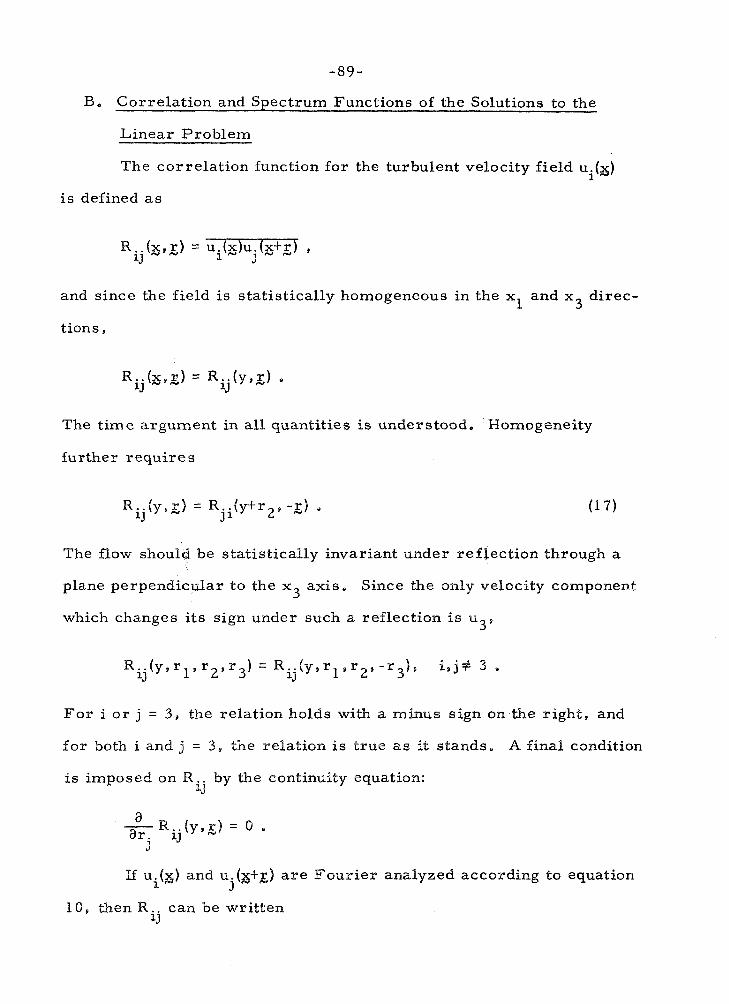
B. Correlation and Spectrum Functions of the Solutions to the

Linear Problem

The correlation function for the turbulent velocity field u.(z) 1

i s defined a s

and since the field i s statistically homogeneous in the x and x direc- 1 3

tions ,

The t ime argument in a l l quantities i s understood. Homogeneity

further requires

The flow should be statistically invariant under reflect ion through a

plane perpendicular to the x axis , Since the only velocity component 3

which changes i t s sign under such a reflection i s u 3 '

F o r i o r j = 3 , the relation ho9ds with a minus sign on tihe right, and

fo r both i and j = 3, the relation i s t rue a s i t stands. A final condition

i s imposed on W .. by the continuity equation: 13

Hf u .(z) and u.(g+r) a r e Four ier analyzed according to equation 1 J

10 , then W . . can be written 1J

Since the left side does not depend on xl o r x3,

The spectrum function A.. defined by this relation depends on kl , kg 1J

and both k2 and k i , since the velocity field i s inhomogeneous in the y

direction. The integrations over k' and k; in the expression for R . . 1 1J

can be performed immediately to give

Since W . . is rea l , 1.l

The symmetry condition l 7 imposes a further r e s t r i c t i ~ n on A.. , since 13

Comparing that with equation l 8,

Aij(kL9 kl k;, kg) = Aji(kZ -kl 9 kZ, -kg) e

The condition on the reflectional symmetry of Rij implies

A..(k;,k19k2,kg)=A..(k;,kl,kZ9-k3). i , j + 3 . U U

61 9 )

-91 -

The incompressibility condition imposes a final restr ict ion -

The linearized solution of the l a s t subsection can be used to

find A.. a s an explicit function of time. F r o ~ n equation 16, 1J

where

and ko denotes the vector (kl.koZ9k3). The expression for A.. a s a 1.l

function of t ime i s now obtained by integrating the equation above over

ki and k; :

A. . (k i ,k9 t ) = Li1 (-kl , k i , -k33kb2) Ljm(kl 9k29k3.ko2) (20) 1J

"k (kbZ9kl.koz.k3) s

where now

kb2 = ki - Ptkl

and

A O Im (kbZ9bo) = Al,(k;z'$. 0) .

-92-

Equations 18 and 20 give R . . (y, 2 , t ) when the initial spectrum function 1J

AO i s known and the linearized equation of motion i s valid. Only I m

R . . (y , 0, t ) will be considered from now on, and in that case the inte- 1J

gration in equation 18 i s more easily ca r r ied out over k' 0 2 ~ ~ 1 'ko2'k3

than over k6. kl , k2 . kg. The Jacobian of the transformation i s 1, since

Thus

In the next subsection, the Reynolds s t r e s s a (y , t j = -R (y, O , t ) i s 2 1

found for a special case where equation 21 simplifies for a rb i t ra ry t .

After that, some general consequences of equation 21 in the limit

a t > > 1 a r e derived.

C . Reynolds S t ress above a Sheet of Random Vorticity

Suppose prior to time t = 8 there a r e no turbulent fluctuations

in the velocity field, and a t t = 8 a random impulse per unit a r ea

f(x, y) i s applied a t y = 8 over the x , z plane. A collection of lifting

surfaces might be shot over the x, z plane a t t = 8, for example.

The inviscid equation of motion for the total velocity x i s

By integrating the equation ac ross t = 0, a new initial field v i s found, -0

where @ i s the impulse of the pressure. The initial turbulent field

u (3) then satisfies '-0

g0(x) + V@ = j f(x, z)6(y) (V

and the continuity condition

Thus go i s a potential flow, u = -V@, for y+ 0. Phillips [4] treated "0

a similar situation in his paper on the potential flow above a waii of

random pistons, an idealization of the flow above a turbulent bound-

a ry layer o r wake. The difference here i s that there i s no wall of

random pistons, but a sheet of random vorticity; there must be a

legitimate veipcity field over al l physical space, Suppose the poten-

tial just above the x, z plane i s @ and just below i s @ Since the y l 2"

component of go must be continuous a t y = 0, equation 22 can be

integrated ac ross y = 0 to give

- @,= f(x9 2)

There i s thus a velocity slip & through the x , z plane given by 0

bo = ‘vl(@1-$92) = 'yf s ( 2 3 )

where V means a gradient in the x, z directions only. After the l

impact a t t = 8, the x, z plane i s covered by a sheet of random con-

centrated vorticity, and the initial tu rbdent flow is potential out of

-94-

the plane. Since there i s no random vorticity beyond y = 0, there i s

no ini t ial Reynolds s t ress . That i s a consequence of integrating the

equation

down from y +a. The problem of the initial random vortex sheet i s

thus ideal for the examination of random vorticity generation by tur-

bulent interaction with the mean field,

The object now i s to find corresponding to the u (5) given "0

by equation 22 and to use equation 21 to find the Reynolds s t r e s s a s a

function of y and t. The Four ier transformations of go, $9 and f a r e

needed, say

where FT1 means Four ier transformation over the x , z plane only,

and 1_ = (kl .kg) Then

and the Four ier transformed momentum and continuity equations a r e

Dotting the momentum equation with S and using continuity gives

In part icular ,

Suppose the spectrum function of f i s I&(&) -

A relationship between I&@) and the spectrum function@ (g) of the

upwash distribution used by Phillips can be found. The upwash a t

y = 0 i s u (x, 0 , ~ ) ; suppose 0 2

But

Thus

where P i s the magnitude of k , and

The large scale contribution to the upwash i s thus isotropic with r e -

spect to rotations in the x, z plane regardless of the character of GC/,

an interesting example of pressure forces leading to isotropy. F u r -

2 thermore, 63 i s 8(1 ) when $-' has a finite value at ,& = 0 . This leads

to a surprising physical conclusion a s follows, 31/ i s the Four ier

transform of the impulse correlation function f (x, z)f(xt , z' ) ,

By inverse Fourier transformation,

f (x , z)f (x' , z' ) d ( ~ - ~ ' ) .

If f satisfies an ergodic property, so ensemble averages can be r e -

placed with averages over large portions of the x, z plane,

q ( 0 ) = Lim

24-00

If the f(x, z ) over separate patches of the plane behave like uncorrelated 7

random impulses, the integral diverges like VA, and $40) # 0. Sirni-

lar ly , 9

But equation 25 requires 0 ( 0 ) = 0 even if q ( O ) $0, Thus a spatially

random impulse generates an upwash with negative correlation be-

tween neighboring patches; in other words, if fluid is slammed down

in one place, i t i s likely to squirt up nearby, Since

from equation 2 3 , the spectral distribution of the slip velocity i s also

2 0(1 ) a s $ + 0 for q ( 0 ) it. O. Phillips used 0 ( 0 ) = O and got results in

good agreement with experiment, but his demonstration for 0 ( 0 ) = 0

was in e r r o r , It i s now apparent that i f the turbulence i s generated

by impulses in the fluid itself rather than by pistons in a wall, 0 ( 0 ) = (9

i s a natural result,

The Reynolds s t r e s s o(y. t) equals -R12(y, 0 , t) o r -RZl(y9 0, t).

The way equation 21 i s se t upp fewer primes have to be written i f R 2 1

i s computed. Since LI3, LZ1 and L23 a r e zero , the integrand for

R21 in equation 21 has the form

L A0 = L L A0 t L 2 2 L 1 2 ~ ; 2 . L 2 ~ lrn I m 22 11 2 1

From equations 24,

where j5' = (kl , kh , k g ) Equations 15 and 21 give the Reynolds s t r e s s

a s a sum of complicated integrals:

o(y, t) = -RZI(y. 0 , t ) = I1 + I2 + I3 ,

klko2 i(ko2+kb2 )Y -- 2 2 , 2 e dkb2dko2q 9

* kok 0

k",: @(I) w I2 i(ko2+kb2)y - [Q] - --- e dkb2dko2dm_ 9

%f3 Ti'

2 k2k'2 0 0

The geometrical quantities appearing in the integrals have been de-

fined under equation 1 5 and in equations 21. The great advantage of

the vortex skeet problem is that the integrals Il and I cancel identi- 3

cally. That is shown in Appendix B, and the integrations over ko2

and kb2 in I2 a r e also carried out to give the final result

The implications of equation 28 become clear when several

limiting cases a r e studied.

(i) Slt 0. Then

so the Reynolds s t r e s s i s zero a t t = 0, a result antici-

pated ea r l i e r , and begins to grow linearly with time.

(ii) Slt -. co. Substitute = 4 I y 1 in equation 28 -

As Qt -+ m, s i n ( ~ t K ~ ) / K ~ behaves like a 6-function of

weight IT in the integration over fcls and except a t y = 0,

provided 0 ( 0 , k3) exists. The case where O(0,k ) does 3

not exist, where al l the initial turbulent vorticity is - aligned in the xl direction, i s discussed in section 4.

F o r a roughly isotropic initial turbulent flow, the

s t r e s s relaxes into a steady distribution except at

y = 0,

(iii) y 0. Hold t fixed and take the l imit y " 0 in equation 28: 9

The Reynolds s t r e s s a t y = 0 grows linearly with time

for a l l time.

-100 - (iv) y + m. Take the limit y " oo in equation 29. Fo r Q small ,

from equation 25. That relation can be substituted in

the integrand of equation 29 except where K i s large ,

and the exponential factor eliminates contributions to

the integral from regions of large K anyway. Thus

- 4 Hence the s t r e s s decreases a s y , for y large com-

pared with the length scale s f the original fluctuations

- 4 for all time. Phillips [4 ] found a y decrease for

the fluctuation mean energy density in his potential flow

pqoblem.

(v) Slt m. y " m. As Qt + oo in the l as t equation, sin(SltK1 ) / K ~

again behaves like a 6 -function, and

The evolving s t r e s s profile i s sketched in figure 4. The details, of

course , depend on a detailed specification s f $E/(J), the spectral dis -

tribution of the impulse, The important point i s that the s t r e s s

relaxes into a steady profile a s Qt becomes large , except a t the

sheet of concentrated vorticity itself, This behavior i s not peculiar

to the vortex sheet problem, but occurs for any (roughly isotropic)

initial conditions, That i s shown in the next subsection,

D. Revnolds Stress in the Limit Q t + m of the General Problem

In the general case , the integrand for R21 in equation 21 still

has the form given in equation 26. Since kt = k' 2 02 + Qtkl from equa-

2 2 tions 21, the factor L = (1 t k 5 ) / ( 1 t kt:) in front of both t e rms 22

in equation 26 forces the integrand to zero a s 52t +a, except in

regions of small kl . But equation 15 shows that the f i r s t t e rm of

L12 has a k in the denominator, and the portion of the integrand 1

containing tha,t factor should give the dominant contribution to the

Reynolds s t r e s s for large times. Thus the Reynolds s t r e s s should

be appr oxima tely

This corresponds to the quantity I2 defined in equations 27 for the

vortex sheet problem. In that problem the other t e rms , I2 and 13,

cancelled identically. Generally they do not cancel, but the fact

that they a r e negligible in the limit a t +m i s established in Appen-

dix C.

Transform the variables of integration in equation 31 a s

Pollows :

ko, = Q ( S 9

k b 2 = l ( S ' 9

kl = l cos@ ,

kj = *sin@

-103-

3 The Jacobian of the transformation i s B . Thus

It can be shown easily that

f(sin@, cos@) dqb = 2 f(sin@,cosqb)d@

Q 0

0 for a function f symmetric on its f i r s t argument. AZ2 i s symmetric

on i ts Past argument by equation 19, so $ may be integrated from 0

to ?r onby, and the resal t multiplied by 2. Now substitute

Then

L sin @ 5 2 cos -V

for 0 G @< n, and the s t ress integral i s

t

o(y , t ) = -2 ( l + p Z ) ( l + p 1 2 ) ~ [ cot - .I (ptg)-cot-lpl

-m -a 0 - a t 5D+(p t -a2]

So far no approximations have been made in transforming the par-

ticular term sf a (y , t ) retained in equation 31. The next step i s to

find the limit of o(y , t ) a s a t "00. The l imit can be taken in the ex-

pression above before an explicit integration is carr ied out if the

resulting integral converges fo r large 5. But the integrand i s of

order c- ' for large 5 , the integral thus converges, and in the limit

00oOoOw 2 3 - 1 o(y,ti =+ -2 J' J' J' J' ( 1 t p 2 ) ( 1 t ~ ' )' cot jp+c)-cot-lP1

-a3 -00 0-00 5[ 1 +@I- el2]

Equation 34 i s the general analog of equation 30 for the vortex sheet

problem and shows that in the general case the s t r e s s relaxes into

a steady profile a s S2t -. oo. Again, the assumption that the initial

0 flow i s 'roughly isotropic, ' i .e. , that A l m ( k ~ , ~ . k Z , k 3 ) exists.

has been made. The same chain of transformations that led to equa-

tion 34 i s used in Appendix C to show that the larges t t e rm left out

of equation 31 i s 0(0t)- ' in the l imit a t .+ m.

The physical situation behind the asymptotically steady s t r e s s -

o(y,t) = - uv can be seen more clearly by considering the mean - 2

square values of pa and v separately, v i s easy to find, since the

integrand of equation 21 for Pi contains only one non-zero t e r m , 22 -

2 ~ 2 2 ~ 2 2 ~ O Z 2 ' The integrand for u contains several t e rms , the domi-

nant one being L L A0 a s Ot .+ m. There i s no point in repeating 12 12 22

the kind of argument which led from equation 31 to 34, Provided

the transformed integral of a t e rm in equation 21 converges a s 5 - - 2 2 n-1

(and it does fo r v o r the dominant term of u ), the t e rm i s 0(Ot)

a s Slt co, where n i s the power of in the denominator of the kl

integrand. A glance a t equation 15 shows that

a s Slt + co. Thus mean field interaction with the turbulence imposes

a heavy veto on vert ical fluctuations but promotes high-speed surges

in the direction of mean flow. This observation was made by Moffatt

for the case of homogeneous turbulence, and was already apparent

from equations 15 and 16. A rough physical description of the pro-

cess goes a s follows. A blob of fluid may be moving upward a t t = 8.

As it moves it tends to retain i t s original speed in the x direction,

but it i s sheared out flat perpendicular to the y axis and loses upward

momentum to the fluid around it, It i s left a s an elongated and flat-

tened slab of fluid lagging behind the mean flow of i ts surroundings. -

The Reynolds s t r e s s -uv becomes steady a s the u fluctuations become

large because of vertical convection, and the v fluctuations them-

selves drop to zero.

Equations 38 o r 34 a r e embarrassing results in a study aimed

a t the propagation of turbulence through mean shear flows, As

Sl + as the turbulence stops propagating, Apparently, any proper-

ties of the equations of motion that would have led to a diffusion of

Reynolds s t r e s s have been lost in the linearization. In the next sec-

tion a more restr icted c lass of initial conditions is considered, and

non-linear effects, in some measure , a r e restored,

4. Flow Uniform in the x Direction

A. The a ~ / a x = 0 Assumption

I£ a roughly symmetrical blob of fluid begins to r i s e , i t i s

elongated and flattened against i ts line of ascent by the mean shear

flow, its apparent mass (associated with displacement of the fluid

around i t ) increases , i t s ra te of ascent decreases , and the blob be-

comes a shaft of fluid lagging behind the mean flow of i t s surround-

ings. This picture i s appropriate if the initial turbulent flow can be

blocked off into roughly symmetrical and independent blobs. The

picture i s meaningless when the original turbulence consists of

eddies uniform and infinitely elongated in the x direction, when

distinguishable fluid blobs a r e columns to begin with. If the original

eddies a r e independent of xs al l flow properties a r e independent of

x for al l t ime, The inviscid equations of motion 1 for the total

velocity x and pressure .rr a r e them

where

-107-

The f i r s t equation states that the x component of momentum of a fluid

column i s conserved a s the column i s transported in the y, z plane.

The next three equations, the y and z momentum equations and the

continuity equation, a r e completely independent of vl and de scribe

the dynamics of two-dimensional, incompressible flow, Given an

initial flow v (y, z ) , v2(y, z , t ) and v3(y, a , t ) a r e found by solving the 0 w

two -dimensional problem governed by equations 3 6 , then v (y, z , t ) 1

i s found by integrating equation 35 using the known histories of v 2

and v Averages a r e taken over a n ensemble of v (y , 2). If the 3' w 0

initial fields have the form

for example, where = iU and the initial perturbation velocity 0

IY 0

- component u (y, Z ) i s zeroI then the initial Reynolds s t r e s s -uv i s

0

zero, and the mean flow profile i s U(y, t ) = v (y, z , t ) for a l l t. The 1

fluctuating par t of the vorticity field which evolves from such an

initial condition i s - not two-dimensional in the sense that the turbulent

vorticity i s aligned in the x direction. The initial turbulent vorticity

i s aligned in the x direction (for uo(y. z) = 0). but the field i t induces - stretches the mean field vorticity and produces a three-dimensional

random vorticity field 2 = ( c , ~ , 5 ) . The assumption that aF/ax = 0

for any flow property F implies only that g = %(yP z ) =

The simplest example of the type of situation studied in this

section i s a line vortex on the x axis in a shear flow with an initial

linear profile v = Qy, The geometry of the problem i s shown in ol

figure 5. Equations 36 a r e satisfied by a steady* tangential velocity

FIG. 5 A SHEAR FLOW WRAPPBNG AROUND A VORTEX

ve = k/2nr, where k i s the circulation around the vortex and r i s the

distance from the origin in the y , z plane. A fluid column a t r , 8 a t

time t originated a t r , 8 a t time 0, where 0

The height y corresponding to i ts original location is r sin 8 , and 0 0

the original and, by equation 35, the final speed of the column in the

x direction i s Oyo. Hence

Set

Then

A contour map of P(p, 0) i s shown in figure 5. The portion of the plane

where p > 0 i s shaded. Pn physical space9 the picture would expand

with fro and the speed a t geometrically similar points would grow

with 6 a s well.

A single vortex thus wraps the initial shear field into an ex-

panding and tightening spiral of speeds of alternating sign, a surpr is-

ingly complicated flow for such a simple initial condition, Suppose

v i s measured over a circular patch in the y, z plane centered a t 1

r , 8 with a radius 6 << r . Initially the speed i s about S2rsine every-

whe re on the patch. As the field induced by the vortex redistributes

f lu id columns, the speed trace over the patch distorts , forms loops,

and eventually goes through high-pitched sinusoidal oscillations in

the radial direction. The amplitude of the oscillations i s f2r over

2 3 the patch, and the wave length A i s 2n r /kt. F o r t so large that

A<( 6 , the average of the t race over the patch tends to zero. As

t -' m, the speed v averaged in the vicinity of any point y, z ap- 1

proaches zero; a single vortex eventually stops the area-averaged

flow anywhere. The radius W inside of which the flow i s 'stopped'

2 in th is sense must satisfy 2nR /kt <<<< 1 SO a B such that A<< 6 << R

can be found. Thus R << 'dx, and r < d- kt /40, say, in the

region of "topped' (but highly striated) flow. The ' stopping power'

of a single vortex thus depends on steady induction over a long in-

t e rva l of time. If the vortex itself moves in a turbulent field, no

such interval i s available, and the picture must change entirely.

What bearing does the a ~ / a x = 0 problem have on the more

general problem, where flow properties depend on x a s well a s y and

z? An obvious answer i s that the 8F/ax = 0 problem can be used

a s a testing ground for approximate theories. The fact that v2 and

a r e independent of v i s an enormous simplification, FOP example, B

consider the linearized problem, the problem solved by Fourier

transformation in section 3, The linearized, inviscid equations of

motion 9 for the fluctuation quantities become

2 2 2 2 when a ~ / a x = 0. The las t three equations imply (a / a y I- 8 / a z )p=O.

Thus p = const. = 0, since p = 0, and the second and third equations

show v and w remain equal to their initial values,

If the initial value of u i s zero , then

from the f i r s t equation. The Reynolds s t r e s s i s

Three steps were required to produce the analog of the resul t that

took al l the algebra of section 3 to derive in general! Notice the

Reynolds s t r e s s grows linearly with t for a l l t ime instead of tending

asymptotically to a steady state a s i t did in the roughly isotropic

case. Equations 15 and 16 show that. the Fourier modes which a r e

strongly excited when P2t >> 1 depend on initial modes occupying the

kl L ( ~ t ) - l / L sector of wave-number space (L i s the length scale of

the turbulence). If a l l the turbulent energy i s loaded into the k2,k3

plane, a s it i s in the aF/ax = 0 problem, then al l the initial modes

remain effective for al l time. In the roughly isotropic case , where

modes a r e distributed over kl , k2, k3 with no singular concentration

in the k2, k3 plane, fewer and fewer of the initial modes remain ef- - -

fective for large t imes , and u2, v2 and grow l e s s rapidly (Moffatt

[ 5 ] presents this argument more quantitatively).

The general problem i s complicated enough even when lin-

earized, It would be extremely hard to use a better approxima-

tion, the mean field equations 8, in a practical problem, But the

mean field equations reduce to a simple form when ~ F / B X = 0. The

las t three of equations 37 a r e the same in the mean field approxima-

tion, so v(y, z , t ) = v (y, z) and i s independent of time. The momen- 0

turn equation for u i s

The result of multiplying the equation through by v and averaging i s

for the Reynolds s t r e s s o(y , t ) = -uv.

The equation of mean motion i s

so the mean field equations lead to a one-dimensional wave propaga-

tion problem with a variable phase velocity Consider the

rather artificial problem sketched in figure 6 ,

-113-

The initial speed profile i s l inear,

- 2 and the turbulence i s confined to a band between y = + h. v equals a 0

constant c2 where l y 1 > h. If the initial s t r e s s is zero everywhere

(that i s , the turbulence i s initially two dimensional, uo(y, z) = 0).

from 39(ii). Equation 39(i) implies ~ ( y , t ) = 0 for 1 1 > he Integrating

39(ii) ac ross y = fi gives the jump condition on o, [o] = 0, so

o w , t) = 0 just inside l y 1 = h. Then from 39(i),

Equations 39(i) and (ii) combine to give

in the region l y I < h , and a general solution i s U = F(y-ct) + G(ytct).

The initial and boundary conditions determine the final result ,

where i i s the periodic function shown in figure 7 . U(y, t ) i s itself

periodic with period &/c . The history of U over one period i s shown

in figure 8,

The rockingp periodic speed profile s f figure 8 cannot be a

good approximation to a real flow, but it i s fa r more plausible than

the equivalent result from the fully linearized equations. From

FIG. 6 TURBULENT BAND BN INITIALLY UNIFORM SHEAR

FIG. 7 THE BER10D861 FUNCTION 4

FIG. 8 SPEED PROFILE ONE PERIOD

-116-

2 equation 38, o = c fit fo r l y l < h , and o = 0 for l y l > h , based on the

full linearization. If this s t r e s s i s used in the mean momentum equa-

tion 39(ii) to find a f i r s t approximation for U (the zeroth approxima-

tion being U = Sly), the result i s

Sheets of concentrated momentum and infinite speed form at y = + h.

This particular problem is physically unrealistic, of course, but it

does show that the mean field equations can give qualitatively reason-

able results when the linearized equations give nonsense. It i s only

in the case a ~ / a x = 0 that the mean field equations can be used with-

out overwhelming aigebraic complexity.

The consequences of any theory of Reynolds s t r e s s generation

can be drawn out much more quickly when the flow is independent of x

than otherwise. The aF/ax = 0 problem i s a t leas t a useful heuristic

analogy to the general problem. Possibly i t may be more than an

analogy. According to the linear analysis of section 3 , Fourier modes

whose wave vectors l ie close to the k ,k plane (that i s , Fourier 2 3

modes which represent eddies nearly aligned in the x direction) a r e

preferred in the sense that they contain most of the turbulent energy

when Qt >> 1. The non-linear t e rms dropped to produce that result

may re tard this tendency to anisotropy, On the other hand, they may

accelerate the transfer of excitation into the preferred modes. Lf

a ~ / a x = 0 for any flow property F, then the velocity correlation func - tion R. . (y,,g) i s independent of r l ; correlation contours a r e infinite

=J cylinders aligned in the x direction. Experiments on turbulent wall

layers , where the turbulence also interacts strongly with a mean shear

flow, show that the correlation functions a r e very much elongated in

the x direction [8 ,9 ] . Even if R . . were completely independent of r l , 13

i t would be impossible to conclude that the flow i s independent of x ,

since higher moments could still depend on spatial separation in the x

direction. But insofar a s the propagation of turbulence in a mean

shear flow depends on low-order statistical moments like Pi.., i t i s 1J

possible that highly sheared turbulence spreads as if the eddies were

independent of x.

Be The Random Vortex Sheet Problem with a~/ax = 0

If the turbulence i s initiated by an impulse concentrated in the

x , z plane and independent of x, the flow i s independent of x for al l

time. In that case the linear and mean field equations for the evolu-

tion of Reynolds s t r e s s , equations 38 and 39, can be compared easily.

The only property of the initial flow required in equations 38 and 39 i s - 2 the mean square upwash vo(y). and that can be obtained directly from

the work of section 3 6 on the generation of an initial field by an a r ea - impulse f(x,z). However, the argument leading to vz is simpler and

more illuminating when f i s assumed independent of x from the begin-

ning, so the argument i s reviewed quickly here.

The equations of motion for the total velocity x and pressure IT

a r e

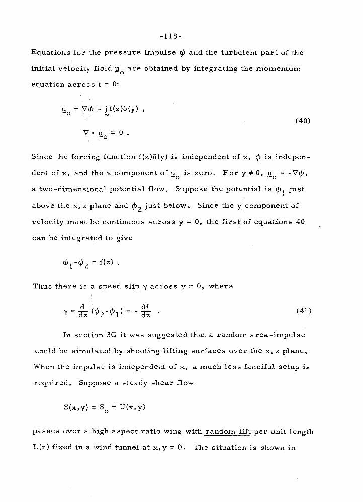
-118-

Equations for the p ressure impulse Q> and the turbulent par t of the

initial velocity field go a r e obtained by integrating the momentum

equation ac ross t = 0:

Since the forcing function f(z)d(y) i s independent of x, @ i s indepen-

dent of x, and the x component of go i s zero. F o r y # 0, so = -V$ ,

a two-dimensional potential flow. Suppose the potential i s just

above the x, z plane and $ just below. Since the y component of 2

velocity must be continuous ac ross y = 0, the f i r s t of equations 40

can be integrated to give

Thus there i s a speed slip y ac ros s y = 0, where

In section 3C i t was suggested that a random area-impulse

could be simulated by shooting lifting surfaces over the x, z plane.

When the impulse i s independent of x, a muck Bes s fanciful setup i s

required. Suppose a steady shear flow

passes over a high aspect ratio wing with random lift per unit length

L(z) fixed in a wind tunnel a t x p y = 8, The situation i s shown in

figure 9 . The speed profile might be linear f a r upstream, S + So+ S2y

a s x + -a, but downstream the flow i s distorted by the random vor-

ticity shed from the wing. The wing delivers a concentrated impulse

-L(z)/so to the fluid passing over i t , and the velocity jump through

the wake is

analogous to equation 41. F o r So much la rger than a typical down-

wash speed, the flow varies only slowly with x , and the time t in the

non-steady problem i s analogous to the ratio X/S . Any results found 0

in the non-steady problem can be turned into predictions about the

wind-tunnel experiment through the prescription

Equation 41 gives the slip speed y as a function of the impulse

f , but it can also be integrated to give the f required to generate a

given y:

f i s forced through a random walk to generate a random slip speed y,

and by the transformation of variables usual in random walk prob-

lem s ,

for y homogeneous in z with a correlation function y(z)y(z+5) = r(5).

f should also be homogeneous, and for z large enough, f(z) and f(0)

should be independent. Then a s z + m

The equation cannot be satisfied for an impulse with finite variance

unless

Equation 42 imposes a severe csnstraint on the kind of vortex sheet

that can be generated by finite and homogeneous random impukses,

or the kind of wake that can be generated by a random wing. Regard-

l e s s of the correlation between neighboring random impulses, even

if neighboring impulses a r e completely independent, the vorticity

over neighboring par ts of the wake must be negatively correlated so

the integral of the correlation function i s zero, The equivalent result

was obtained for the general problem in section 3C, but not so

directly.

Equations 40 can be solved by Four ier transformation just a s

before. Thus if ? (kg) i s the Four ier t ransform of f over z and

a (k k ) i s the Four ier transform of go over y and z, -0 2' a

where 5 = (k2, kg). In particular

and the upwash a t y , z i s

Suppose f has a spectral distribution *(kg), so that

Then the initial upwash correlation a t a height y i s

The spectral distribution of the upwash a t the vortex sheet @(kg) i s

the Fourier transform of Q(8, &), Thus

k: @(kg) = - 4 *(k3) 9

analogous to the general result discussed in detail in section 3C. In

order to get a specific result , suppose

Then

-123-

Finally,

- Now that v2 is known, the s t r e s s can be computed according to the

0

linear approximation , equation 38, o r the mean field approxima tion,

equations 39, - In subsection A i t was shown that a discontinuity in v: leads

to the formation of a sheet of concentrated momentum under the linear

approximation. According to equation 38,

for the vortex sheet problem. a i s continuous but has a discontinuous

f i r s t derivative with respect to y a t y = 0. This time, the f i r s t ap-

proximation to the mean speed,

jumps across y = 0. This more modest singularity i s stil l unaceept-

able. Any such jump must be preceded by a steepening of the speed

profile near y = 0, but the integration of the momentum equation for

u to give u = -Qtv in the derivation of equation 3 8 , requires to 0

be constant in time,

The mean field equations 39 give a more realistic resul t ,

since they do take into account the change of mean speed that invali-

dates the Binear approach, Suppose non-dimensional variables a r e

defined a s follows:

Then equations 39 transform to

The Reynolds s t r e s s i s non-dimensionalized on the typical mean

speed S times the fluctuation speed c. Lf the flow i s 'highly sheared, '

2 S > > c , then a > > c . Random stretching of the mean field vorticity

produces a s t r e s s much la rger than the original turbulent energy

density. The t ime characterizing changes is properly non-dimen-

sionalized on l / c ; in a time of order l /c the mean flow reacts to the

s t r e s s , But I/@ i s also the time scale for non-linear convection of

turbulent vorticity, the phenomenon neglected in the mean field

approximation, Thus the mean field equations a r e not a consistent

approximation and can give only a qualitative description of the real

flow.

If 1 , c and % a r e related to p A and %% by the equations

then the non-dimensional form of equation 44 i s

and the initial and boundary conditions a r e

k im r ( q , ~ ) = ? 9 ITJ -+GO

for a mean speed profile linear a t t = 0. Equations 45, 46 and 47

determine the history of the flow according to the mean field approx-

imation lCor al l time.

The mean field equations a r e only a qualitative approximation

for any time t , and for t large compared with the turbulent convection

time 8 /c , they must be a bad qualitative approximation. The cylin- -

2 drical eddies inducing the mean square upwash v themselves disperse

- 0

after a time of order PIC. Assuming v2 i s unchanging for a l l t ime led o

to the peculiar periodic solution of figure 9, Thus the solution to

equations 45, 46, 47 i s relevant only in the l imit T < < 1, h that case

it i s reasonable to rewrite the problem in t e rms of an expanded

coordinate

-126- N N

and t ry to find asymptotic se r ies expansions of r (q , T;E) and s(q , T; E )

in powers of E . In Appendix D, i t i s shown that the expansions begin

the same a s the linear solution. However, the ordering of the t e rms

breaks down where q ~ E , and in that region i t i s necessary to use a

second expanded variable

A function g which is symmetric and peaked like the function in equa-

tion 46 can be expanded around q = O in the form

If g = (1 + 1 q1 )- 3 , a = 3. It i s shown in Appendix D that equations 48 N 01

a r e correct even for small a s long a s lq 1 > T, and that the expan- N w rV IV

sions for s(q, T;E) and r (q , T; E ) begin

where I';i 1 < T. To second order in E, the singularity at the vortex

sheet affects only the portion of the q, T plane between the particular

zeroth-order characterist ics, q = $ T, which originate at q = 0 when

+ = 8, Expansions 48 and 49 become

when rewritten in t e r m s of the original non-dimensional variables

q , T. The non-dimensional s t r e s s s (q , r) and speed change r (q , T) - r (q , 0) = r (q , 7)-q a r e sketched in figure PO. In the region q I < T

where the l inear and mean field results differ, the linear resul ts

a r e shown a s dotted lines.

The speed slip of the linear approximation i s patched up in

the region Iq 1 < a$ and the mean field profiles a r e plausible. How-

ever , the sheet or" concentrated vorticity that generated the peaked -

2 vo (y) at the s ta r t must wrinkle and occupy the band 117 1 < T itself. - 2

vo(y) should be blunted about a s fast a s G so the mean field approx-

imation i s suspect in the only region it makes any difference, That

i s inevitable, The mean field approximation i s not consistentp and

the only advantage it has over the full linearization i s that i t gives w

2 more reasonable results near singularities in v (y),

0

The l imits of s and r for a >> l can be found by Eaplace t rans-

formation of equations 45, 44 and 47, One result i s that r (q s 7)-0

for q fixed and -r4m; the flow i s eventually stopped anywhere. If

the result were t rue i t would mean random eddies exert a sustained

grip on the mean flow. In fact the result i s worthless, The grip

loosens rapidly a s the eddies disperse in their own turbulent field.

An entirely different kind of problem involving sustained induction

i s treated in the next subsection.

C. Steady Induction by Line Vortices of Alternating Sign

Any physical app rox im tion which neglects non-linear inter - action between turbulent eddies leads to the conclusion that the mean

flow stops anywhere after enough time. In the = 0 problem,

the x component of momentum i s conserved in fluid columns (equation

35) and i s diffused by turbulent motions passively, like heat o r chem-

ical concentration. Without dispersion of the eddies, the intensity of

turbulent mixing i s constant in t ime, and regardless of how slow the

mixing i s a t any particular height, given enough time i t i s sufficient

to diffuse away any mean momentum gradient. The important ques-

tion i s , how much time i s required to stop the flow? If the time

needed were small compared with the turbulent convection t ime, the

flow would indeed be stopped, but that i s impossible since the mo-

mentum redistribution is i ts elf a convection phenomenon. The tur -

bulent eddies should disperse a t about the same rate the x momentum

diffuses, and the mean flow should be more o r l e s s distorted, but not

stopped,

One situation where there - i s no convection of initial vorticity

was described in subsection A - the case of a single vortex aligned

on a streamline of an initial l inear shear flow, There the flow is

9stopped,v not in a statistical sense, but stopped in the sense that

the x speed averaged over a patch of finite a r ea tends to zero a s

-130-

t - a>. Suppose that instead of one vortex there i s an infinite s t ree t

of vortices of alternating sign aligned paral lel to x and distributed

along z a distance h apart. The setup is shown in figure 11. The

vortices a r e in equilibrium, since the velocity a t any particular vor-

tex induced by al l the others i s zero, The equilibrium is unstable,

but in principle the vortices can remain in their original locations

and steadily redistribute the x momentum of an initial l inear shear

profile. Fluid columns move in roughly elliptical orbits a s shown.

Since the orbit t ime differs from streamline to streamline, fluid

columns crossing line A-A a t a large time t may have originated a t

greatly different heights even if their current separation i s small.

A speed t raverse along A-A in figure 11 eventually shows high-pitched

oscillations, and the x velocity component averaged over an interval

X at a constant height y becomes small a s t +- ao, This flow i s

nothing like non-steady turbulence, but i t i s homogeneous in the z

direction, and the t ime i t takes to stop the line-averaged flow here

may give some indication of the time required by turbulence to stop

a flow in the statistical sense,

Loops in the speed t raverse along A-A a r i s e after a t ime

comparable to the orbit time in the trajectory tangent to A-A, T(y)$

the orbit t ime in the trajectory whose apogee i s y , i s thus a lower

bound on the time needed to stop the line-averaged flow a t y, The

object here i s to find T(y).

Since the flow in the y, z plane i s dynamically independent of

the x momentum i t t ransports (equations 361, i t can be treated a s an

incompressible, two-dimensional flow. It i s irrotational a s well,

-132-

except a t the vortex singularities. Thus a potential @ (y, z ) and

s t ream function +(y, z ) can be found such that

and each location in the y, z plane can be assigned potential and

streamline coordinates @, +. Suppose the speed

v = v 7 -

i s known in t e rms of @, +. If s measures the a r c Eength along a t r a -

jectory (streamline) specified by +, then

V also satisfies

Thus

The time i t takes a fluid column to move from potential q5 to poten- 0

t ial @ along the trajectory specified by + i s B

Notice t i s positive, since @ must always decrease in the direction

the fluid column moves. Each orbit encloses a single vortex of

strength + k. As a column orbits once, the potential decreases an

amount k , so the orbit t ime around the trajectory specified by + i s

The value of + on the trajectory with apogee y i s +(y, 0), Thus

and the problem of finding T(y) i s solved in principle.

Complex variable notation makes an explicit solution sus-

prisingly easy, The details a r e given in Appendix E. The result i s

with

k s i d +(y, 01 = -i;; log

l + cosh 9 (1

x

Two limits a r e especially interesting:

2 2 P

2kz e ~ ~ / x @ a s y X'ao, T(y)*F (i

The orbit time a t a radius y around an isolated vortex of strength k

2 2 i s 4n y /k, the same a s limit a. A fluid column very close to a

particular vortex i s hardly affected by the other vortices in the street .

Limit b i s the surprising result. The orbit t ime around a trajectory

with apogee y i s exponentially large for large enough y. The two

limiting cases of equations 51, derived for y << X and y >> A, give

practically the same results for intermediate values of y. F o r

y = X / 2 , l imit a i s

and limit b i s

The limiting expressions agree very well around y = k / 2 , the apogee

of the orbit with major axis )I. Beyond that orbit, l imit b must be

an excellent approxirnatiois. Thus T(y) , a lower bawd on the time

required by the vortex s t reet to decelerate the Pine-averaged flow

a t a height y, grows exponentially beyond y- X . The ra te sf mixing

x momentum i s zero, for al l practical purposes, outside the imme-

diate neighborhood of the vortex street ,

The apogee of the orbit that has been completed just once by

time T is

X kT Y = - log - IT 2XZ

for Y 2 X , Y ( T ) i s the height of the @frontg where the line-averaged

-135 - flow i s being significantly decelerated a t t ime T. The front propa-

gates a t a speed 'i = X/TT. But the slightest disturbance destroys

the equilibrium of the vortex s t reet and allows the vortices to d is-

2 perse a t an initial ra te k/X. By a time of order X /k, the vortices

have dispersed past the front they a r e supposed to be forcing steadily

through the flow. Thus no such front can develop in the f i r s t place,

and the result for steady induction by a vortex s t reet can give no

indication of what happens in a real flow. The propagation of turbu-

lence in a mean shear flow cannot be understood without considering

the non-linear action of turbulence on itself. Any analogy, like the

steady vortex s t reet , o r any approximate theory, like the mean field

equations, which omits turbulent convection of random vorticity must

lead to fundamentally unrealistic results. The mechanics of turbu-

lence propagation through a mean shear flows i s inseparable from

the mechanics of the mean flow itself, and any approach which ne - glects mon-linear interaction between random fluctqations will give

a qualitatively wrong description of the mean flow,

5. The Numerical Experiments

A. Basis of the Numerical Approach

According to the l inear approximation of section 3, Reynolds

s t r e s s stops propagating through a mean shear flow once the original

turbulence i s highly sheared. In section 4, the problem was simpli-

fied by assuming al l flow propert ies a r e independent of x , and the

non-linear interaction between turbulence and the mean field was

restored. It was found that no such part ial account of non-linear

convection can give even qualitatively cor rec t resul ts for l a rge times.

Eliminating turbulent convection of random vorticity in the aI?/ax = 0

problem leads to a turbulent field steady in the y , z plane with a

steady gr ip on the mean flow. Under such an approximation, the

mean flow eventually stops anywhere, but in fact the turbulent eddies

d isperse about a s fas t a s the mean flow decelera tes , and the mean

speed profile i s distorted, but not driven to zero. If the propagation

of turbulence through a mean shear flow i s to be understood a t a l l ,

non-linear action of turbulence on itself must be considered, But

the fully non-linear problem i s intractable. Without analytical sup-

port or the support of experiments on the propagation of f r e e turbu-

lence in shear flows, a guess about the effect of non-linearity would

be a rb i t r a ry , Some kind of experiment i s needed,

The outstanding simplification of the a ~ / B x = 0 problem i s

that eddy motion in the y , z plane i s dynamically independent of the

momentum i t convects, The motion i n the: y, z plane can be treated

like two-dimensional turbulence, and the speed in the x direction

like a sca lar quantity convected in a two -dimensional turbulent field,

That does not mean that the only random vorticity in the flow i s the

initial vorticity. All three components of the random vorticity

g = ( S , ~ , W ) a r e generated by mean field stretching. It means only

that the velocity field in the y , z plane i s unaffected by random

stretching of the mean field vorticity. If the vorticity c(y, z , t ) i s

given, then the two-dimensional velocity field = (v,w) can be found

from

where = j (y-y') + &(z-2') . F r o m equations 3 6 , N

a 5 (ii) - t x %.5 = 0 a t

and the integral and differential equations can be solved step-by-step.

If the vorticity i s not distributed smoothly in the y , z plane

but i s packed into discrete vortex columns 9 the problem looks even

th simpler. Suppose the clockwise circulation around the j- vortex

viewed toward negative x i s k Equation 52(i) becomes j

th where the j- vortex i s located a t [y.(t) , z j ( t ) ] , and r = j(y-y.) f 3 J

S ( Z - z . ) . Each vortex i s convected in the field induced a t i ts location J

by all the others, Thus

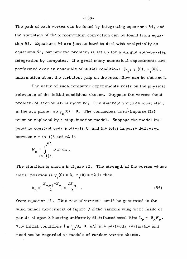
The path of each vortex can be found by integrating equations 54, and

the statistics of the x momentum convection can be found from equa-

tion 53. Equations 54 a r e just a s hard to deal with analytically a s

equations 52, but now the problem i s se t up for a simple step-by-step

integration by computer, If a great many numerical experiments a r e

performed over an ensemble of initial conditions {ki, yi(0), zi(0)},

information about the turbulent grip on the mean flow can be obtained.

The value of such computer experiments r e s t s on the physical

relevance of the initial conditions chosen. Suppose the vortex sheet

problem of section 4B i s modeled. The discrete vortices must s ta r t

in the x, z plane, so yn(0) = 0. The continuous area-impulse f ( z )

must be replaced by a step-function model. Suppose the model im-

pulse i s constant over intervals A , and the total impulse delivered

between z = (n-9. )A and nX i s

The situation i s shown in figure 12. The strength s f the vortex whose

initial position i s y.(O) = 0, zi(0) = nh i s then 1

from equation 41. This row of vortices could be generated in the

wind tunnel experiment of figure 9 i f the random wing were made of

panels of span A bearing uniformly distributed total lifts L = -S F n o ne

The initial conditions { mn/h, 0, nh) a r e perfectly realizable and

need not be regarded a s models of random vortex sheets.

If the vortices kn a r e to be generated by random, homogeneous

impulses Fn of finite variance, then neighboring vortices cannot be

uncorrelated. The proof i s about the same a s i t was in the contin-

uous case. From equation 55,

Thus

Fo r N large, IFNtl and F a r e independent, and the left hand side i s - 4.

2 2 2 F . If the variance of k is k and the csrrelatisn function R is de- n

fined by

then

a s N -. a, The original sum over m and n has been transformed

a s shown in figure 13, Thus

and the relation cannot be satisiied for large Pd unless

FIG. 12 STEP- FUNGUION IMPULSE

FIG. 13 METHOD FOR SUMMING R ( n - m ) OVER n,m

The ensemble of vortex strengths must satisfy equation 56 i f the

computer experiments a r e to represent physically realizable situ-

ations.

If the impulses Fn a r e independent, then nearest neighbor

vortices only a r e correlated, Thus

The correlation function R satisfies

consistent with equation 56. Nearest neighbor correlation was gen-

erally used in the computer experiments. A finite row of vortices

must be used in any experiment, and correlation of nearest neighbors

alone gives the maximum number sf correlation lengths possible

for a given number of vortices. If the correlation does not extend

over a large number of vort ices, the vortices can be taken to repre -

sent large scale eddies in the continuous problem9 rather than ele-

ments of a vortex sheet.

-142-

F rom equation 53, the initial upwash above a row of such

vortices i s

Thus

The upwash correlation above the discrete vortices i s not independent

of z . The flow i s not homogeneous in z because the vortices have

special determinate locations z = nh. However, the upwash corre la-

tion i s periodic on z with period X, so an average correlation

can be used. ,Then

By contour integration in the complex plane,

If nearest neighbor vortices only a r e correlated,

In section 4B, an expression fo r the upwash correlation Q(y9 5) for

the continuous sheet was derived assuming the impulse spectrum

= A exp ( - p, /kg 1 ) In the limit p/y ' 0, equation 43 for Q(y9 5 )

becomes identical to equation 57 if

Furthermore, a s X/y ' 0. v (y,z)vo(y,z+&) should become insensi- 0

tive to z and approach Q*(y, 51, A11 the colrrelations R . . between 13

points in the potential flow region above y can be found from 8 (y, 5).

Thus discrete vortices with neares t neighbor correlations only give

a fa r field which is identical to the Par field of a continuous sheet.

Hn subsection B a way of generating random vortex strengths

2 satisfying k k = k R(n-m) for any R i s described. Once a particu- m n

l a r initial condition i s chosen from the ensemble {k (0)9 zn(0)] n9 'n

the finite difference forms of equations 54 have to be solved step-by-

step for a s many time increments a s a solution is desired, The

computation i s inherently unstable, and the computed vortex Poca-

tions drift away from the locations that would be assigned by an

exact solution, In computer work on deterministic problems, for

-144-

example the work of Abernathy and Kronauer [I11 on the formation

of vortex s t ree t s , this mechanical e r r o r drift i s a serious matter

and has to be kept small by using extremely small time increments.

Here the object i s not to follow detailed vortex paths, but to find

averages over a large number of runs. Each numerical experiment

can be much sloppier than the experiments of [ 11 ] ; each one must

be sloppier i f a large number of experiments i s carr ied out on a

limited budget. Subsections C , D and E a r e devoted to an analysis

of mechanical e r r o r drift , a discussion of how rapid a drift i s per-

missible, and a description of a mechanism for counteracting the

dispersive effect of e r r o r drift of general physical interest - vortex

capture, In subsection F results for some numerical flow visuali-

zation experiments on the motion of random vortices a r e presented,

The flow visualization experiments show how vortices dis-

perse: vortices pair up into dipoles and 'boil' out of the turbulent

region. But no idormat ion i s obtained about the ra te x momentum

is redistributed by the field induced by the vortices. Suppose the

initial shear flow is l inear, t J = Qy, and turbulent velocity fluctu- 0

ations in the x direction a r e initially zero. If the experiment were

conducted in a wind tunnel, a hot-wire measurement could be made

a t y , z a t time t , If the hot wire intercepts a fluid column which

originated at y then the speed i t measures i s Qy (y, z , t ) , since 0 0

the momentum and speed of fluid columns i s conserved, The mean

speed i s then U(y,t) = ~ l c ( ~ . t ) where the average i s taken over a

t raverse along z o r over an ensemble of independent experiments.

But the computer cannot tel l the original height of the fluid column

at y, z a t time t unless a tes t particle ca r r ied along with the flow

from time zero happens to have landed there, In order to simulate

a hot-wire t raverse by computer, tes t particles labeled by their

initial heights y must be scattered over the y, z plane, and their 0

paths computed along with the paths of the vortices. At time t the

particles lying near y a r e surveyed to find their original heights y , 0

If the flow is incompressible and the test particles were originally -

scattered uniformly over y, z , then the mean speed i s U(y, t ) = Q,<(y,t)

where the double-bar average i s taken over the particles surveyed

a t y, t in each realization of the flow and over an ensemble of initial

conditions. This idea i s described in detail in subsection G, and

the results of a se r ies of numerical momentum transfer experiments

a r e presented in subsection HI.

B. Generation of Random Vortex Strengths with a Specified

Correlation

The object i s to generate a large number N of vortex strengths

2 kn which satisfy kmkn = k R(n-m) for any R desired. The average i s

taken over an ensemble of se ts (k n = 1,. , , , N) generated by the no

technique described here. The numbers k a r e taken to be periodic n

with period N, so kN+l = kp for example. Vortices near the ends of

the sequence n = 1 , , , . , N a r e then correlated, but that should make

no difference in the turbulence experiments if N i s much greater

than the maximum I for which W ( 1 ) i s non-zero. F o r nearest neigh-

bor correlation, only the end vortices 1 and N a r e unnaturally corre-

lated, N i s assumed odd throughout the derivation to keep the work

tidy.

Suppose n i s regarded a s a continuous variable. Then any

well-behaved rea l function k(n) of period N can be written a s a Four-

i e r se r ies

where c* = c Where n i s an integer, m -m

Set M = (N-1 ) / 2 . Then

since, for example, cMtl = c N-MP etc- Define

Then

and a periodic function defined on an integer argument can be written

a s a finite Fourier se r ies (cf. Brillouin [ 12 ]j ). The correlation

function can now be expressed as a Four ier transform - Zni

2 -i;j- (pm+sn) k R(n-m) = k k = a a e m n P q

Since the left hand side depends on (n-rn) only,

2 * where 01 = a a The relation between R ( Q ) and a! can be inverted P P P* P

by using the identity

Thus

and M m l -2ni - u2 m =Gc R ( Q ) e N ,4

.I. -P

Jf R(B ) i s given, = a a can be computed from equation 59. I£ m m

random Fourier coefficients a can be generated satisfying a a = rn m n 2 .'.

a! 6(mtn) and a ' = a , then sets of properly correlated random m m -m

vortex strengths can be found from equation 58.

From equation 59,

If the row of 2MtB vortices i s to represent turbulence homogeneous

in z , R(B) must drop to zero long before ( Q 1 - Me Then equation 54

L requires La! = 0, Write 0

-148- - where @m i s a real amplitude satisfying $ = 01 and Om i s a random

m m

phase between 0 and 1. Since em = -8 and a. = 0, equation 58 be- -m

comes

nm k = ), qlm C O S 2'(- + 8 ) . n N m

and each Om i s independently assigned one of the values i ""

at random, then the Fourier coefficients do satisfy aman 2

=a! 6(m+n): rn

It i s interesting to note that the famous random phase, which plays

so large a par t in qualitative discussions about turbulence and no

par t at al l in quantitative theories, i s introduced here to se t the

initial conditions for the computer runs,

The way of selecting @m and Om in equations 60 may seem

inflexible, and it might be thought that the probability distribution

-149 - for k would be a rickety step function. However, there a r e four 0's n

to choose f rom, and M choices must be made to sum the f i r s t of

equations 60. If the number of vortices N = 51, say, then M = 25

and the ensemble of possible initial conditions has

members! The variety seems adequate. Since each k i s the sum n

of 20 o r 30 independent random variables of s imilar variance, the

probability distribution fo r k should be very nearly Gaussian. In n

practice, the values of 8 for m = 1 , . . . , M in each computer run m

were chosen by flipping a coin (twice per 8 ) o r rolling dice. The rn

random phases were then fed into a subroutine which computed k n

according to equations 40. The subroutine was named VEGAS, of

course.

C. E r r o r Drift

Suppose a passive particle has a position = by, z ) at time t.

Given the current vortex locations, the computer can calculate the

velocity ~ ( 8 , t ) of the convected particle exactly (within round-off

e r r o r s ) from equation 53. If the time increment i s T, then the com-

puter assigns a new location 6 -+ 63 to the particle at time t + 7, where

But an exact solution would give

-150-

where the integrand i s evaluated at the changing location of the par-

ticle, Thus the computed trajectory and the ' rea l ' trajectory diverge.

If the particle i s convected in the field of a single vortex, the

computer trajectory can be predicted analytically. Geometrical

quantities a r e shown in figure 14. If the current radius from the

vortex of strength k to the particle i s r , the particle will be advanced

a distance

after a time increment T along a straight Pine tangent to the circle

of radius r. Thus the radius increases a distance b r , where

Then

since 68 = 6s / r . For T small enough, the difference equations can

be written a s differential equations for the computed trajectory r ( t ) ,

8(t):

-152-

If the particle s ta r t s a t r (0 ) = r 8(0) = 0, then the equations give a 0 '

trajectory

(ii) 8(t) = - 2n r

0

2 F o r r+ 0 and t fixed, r ( t ) + r and 0(t) +kt/2nro, the expressions for

0

the actual trajectory. But a s t +a, r grows a s t1/4 and €3 slows

down to a t l l2 growth a s the particle slides out into a weaker ve-

locity field. A numerical flow visualization experiment was per-

formed to check the trajectory predicted by equations 42. A time

2 2 increment z one-twentieth of the actual orbit time T = (2n) ro/k was

used, T = .05T, and the program was run up to t = 2T. The curve

r ( t) /ro from equation 42(i) is plotted against t / ~ in figure 14 along

with the experimental points. The agreement i s excellent (the

oscillation in the experimental data a r i s e s because the points a r e

taken from an on-line computer plot, and a finer spacing is available

across the print-out sheet than down it). There can be no doubt that

the approximation ,tjx = ~ ~ ( 3 , t ) causes the dominant e r r o r in the

numerical experiments,

h the general case, suppose the ' r ea lg position of a particle

a t time t i s _x and the computed erroneous position i s ze. The com-

puted position a t t ime t f T i s then

and the actual position i s

a s shown in the sketch.

But

Bv N

x[l(o). IS] = s(?/, t ) + 2. C1x (5, t ) + (IS-t) W (59 t) + 9 . . 9

where 2 i s the displacement of the particle from ~4 a t t ime IS. Then

and

The expansion can be used in the equation for ys to give

where 3 = Dx/Dt i s the acceleration of the particle at time t, The

computer result can also be expanded in the form

Define the e r r o r vector g = z -315. The expansions for zk and 3' can e

be subtracted to give

for the new e r r o r vector E ' . Thus

Provided T i s small compared with the time scale of the flow and 1% 1

i s small compared with the typical length, that can be written a s a

linear differential equation for g ,

with

~ ( 0 ) = 0. N

Equation 4 3 i s the fundamental equation for the machine e r r o r drift

E , good before g extends clear ac ross eddies and whenever the time N

increment T i s reasonably small* The acceleration term catalyzes

the build-up of e r r o r ; computations based on 63 = cannot keep up

with an accelerating particle, and the computed position slips back

along the line of acceleration. As s increases, the, velocity a t the

computed location becom es significantly different from the velocity

a t the actual location, and the two locations shear apart. Equations

61 for the computer trajectory around a single vortex show the same

behavior, The computed location slips outward a t a ra te 7-12 t imes

the current centrifugal acceleration, The angular speed a t any

radius i s the same a s i t would be for an actual particle, but a s the

computed radius grows, the computed angular displacement lags

far behind the actual displacement,

Equation 63 holds for any velocity and acceleration fields X;

and g specified continuously a t the actual particle location. The

steady velocity and acceleration around a single vortex drive the

e r r o r up continuously and rapidly. But in a turbulence problem

V X and 3 a r e random functions of t ime, and i t might be conjectured

that the e r r o r drift i s l e s s drast ic in that case, more like a random

walk than an exponential divergence. Equation 63 cannot be solved

analytically in closed form, but the conjecture can be tested on a

simple one -dimensional model,

where ~ ( t ) i s a stochastic function analogous to a strain ra te and

P(t) is - r / 2 time,s an acceleration, Equation 64 describes the e r r o r

in computing particle location in a non- steady one -dimensional

channel flow, for example. The object now i s to find the variance - of s , e2( t )$ where the average i s taken over an ensemble of his-

tories ~ ( o ) , P(o), OSoSt,

The exact solution of equation 64 is

Thus

Then

2 Assume /3 i s statistically homogeneous, so that . m j = P B(o-T) . The variance can then be written

- t T 2$crdt1 $crdtl

E 2 = P2 ('dT ('do e T o

e B((s-T)

Assume a ( t ) i s s tr ict ly stationary, and ~ ( t ) and a ( t t T ) a r e indepen-

dent for T > 8. Then for t >> 8,

By substituting x = t--r, y = T-o in integral @ and x = t-o, y = o - r in

integral (6J i t i s easy to show that

X F o r t >> 8, the integrals 1 lYdtv and adt ' a r e ca r r i ed out over many

o P 0

correlation t imes s f a almost everywhere in the domain spanned by

x and ye Thus

for example, i s a random variable of mean zero (assuming has

zero mean) and has a Gaussian distribution (by the Central Limit

Theorem) for - almost al l x in the integrand of equation 65. But n

2 fo r Gaussian X. If (Y(t)a(tl) = (Y A(t-t ') , then

03

fo r almost al l xp where j A(t)dt = 63, Equation 65 becomes

Define the weighted correlation time for P, 00 2

-3a OY 3 = e NY) dy

0 Then for t >> 8 (the dependence time of a ) , O (the correlation time

for (2, presumably " 8), and 3 (the weighted correlation time for P),

F o r stochastic @(t) and P(t), equation 64 represents a generalized

random walk for ~ ( t ) . Under the very stringent conditions assumed - 2

to solve the problem, the variance E i s given by equation 66. The

variance diverges exponentially. It diverges even faster than the

solution of equation 64 for constant a ( t ) = a! if 2 a O > 1. Notice if

the strain t e r q in equation 64 i s either very weak, @ + O , o r varies

extremely fast , 0+ 0, equation 66 reduces to the standard random

walk result

until very large times.

The conjecture that the computer e r r o r given by equation 63

diverges slowly for stochastic x and 2 must be wrang. A numerical

experiment cannot reproduce the detailed trajectories of vortices

and tes t particles for very long times. But in a turbulence experi-

ment the detailed r e r c rd i s not important. A s Bong a s the cor,puted

motion of a particle i s governed primari ly by the flow velocity x a t

i ts current location, the accumulated e r r o r should be unimportant

in a turbulence experiment. The computed location should be just

a s good a s the actual location. Jus t beyond their point of intersec-

tion, a computed path diverges from a physical path with an e r r o r

velocity v given by " E

- T

x, - - - 2 2

from equation 63. A numerical turbulence experiment is valid ii

regardless of detail differences between the computed flow and the

physical flow with the same initial conditions. 6 i s estimated for a

random distribution of independent vortices in subsection D,

D. Flow Velocity and E r r o r Velocity

The model studied in this subsection i s artificial, just a s

equation 64 with statistically stationary a! and (3 i s an artificial model

of equation 6 3 with inhomogeneous vector fields I: and 2. The object

is to show quqlitatively that wi+&out special precautions condition 57

may not be satisfied no matter how small a time i9crement T i s used.

th Suppose the i- vortex has strength k. and location y z . and 3. i i

a passive particle subject to a physical velocity and e r r o r velocity

V-E i s located a t y , z. Define

Gi = z - z i

From equation 53,

ki Gi ki vi V = - -

ZIT r Z 9 W = - -- ZIT r Z a

i i i i

Thus

Now assume ki and k. a r e independent for i # j. That cannot be t rue

for the problem solved by computer in this chapter, since the vortex

strengths must be correlated to satisfy equation 56, Assume that

the location of each vortex i s independent of i t s strength, and that

. Neither of

those assumptions can hold for vortices located initially a t y = 0,

z = nX. By the f i r s t two assumptions, an average over an ensemble

{ki, yi, zi 1 gives

- 2 where k.k = k 6... The e r r o r velocity v equals - ~ $ / 2 ~ and

1 j u -E

The las t t e rm on the right i s zero, since 5, the component of vor-

ticity in the x direction, i s zero outside of the vortex singularities.

The variance of aX/at would be hard to find, but the acceleration 2

L should be the same order a s i ts convective par t B(x 12). The var i -

ance of the e r r o r velocity

can be found about the same way equation 49 was found, but the alge-

bra i s complicated, and the derivation i s deferred to Appendix F,

Under the three assumptions stated above equation 6 8 , the result i s

P

2 T2 k Z,, =

The averages in equations 69 and 70 a r e to be taken over an ensemble

of vortex locations IYi, zi} with the particle position fixed.

Equations 69 and 70 both give infinity if the vort ices a r e d is -

tributed with uniform density over the y , z plane, But suppose - N

vort ices a r e distributed uniformly over an annulus around y , z of

inner radius s and outer radius S. The density of vort ices pe r unit

a r e a is

and the probability distribution function fo r rl, . . . , r i s N

since the vort ices a r e distributed uniformly, where

O otherwise.

Thus

Similarly ,

F o r fixed p and large S and N, the result of integrating and summing

- 2 7 k 4

2 S + 2Ti2 5 log; & C =-T (z)

s

Non-dimensionalize p with the a r ea excluded around each vortex,

Then the ratio of equations 72 and 7l i s

- 2 2

4 S & c 3 Tk

1 + p:: log- - 6' = - - - S

* - k"---$ S c 2 l 6 2as log - X s

Since 6c - 6 , equation 67 implies that the condition 6 << 1 must be c

met for a numerical turbulence experiment to be valid.

What counterparts do S, s , p:g have in a numerical experi-

ment? The computer can handle only a finite number of vortices

distributed over a finite a r ea off the y, z plane, and S can be taken

a s a linear dimension of that a rea , r; i s a distance of closest ap-

proach to a vortex, but it i s not obvious that such a distance has

any physical meaning. One thing i s certain: if s could not be estab-

lished physically, i t wouPd have to be incorporated in the computer

2 program anyway. 6 i s proportional to ~ k / 2 n s , and that combination

C

-163-

must be small in a valid numerical experiment.

It may be that a passively convected particle has a hard time

getting close to a vortex if it i s not close a t the s tar t . As a particle

approaches a line vortex, i t s motion i s dominated 'by that vortex,

and it tends to orbit a t a constant radius. In the case of two ap-

proaching vortices, the argument i s more solid. Equations 54 can

be written in Hamiltonian form (Lamb [10 1 ) ,

where

w = 1 k.k. log r.. , 1 J 1.l

and

r . . = U

and the Hamiltonian W is conserved. No single r.. can become very 19

small. unless an unusually large par t of the energy W is concentrated

in the interaction between i and j. Since such a concentration i s im-

probable in a turbulent flow, close approaches a r e r a r e ,

However, Abernathy and Kronauer, in their numerical ex-

periments on vortex- s t reet formation [l 1 ] # found that vortices of

the same sign tended to cluster into loosely packed clouds, The

important aspect of the flow i s the motion of the clouds in the general

field they induce, rather than the detailed motion of the vortices in-

side, If the computations were done by hand, clouds could be treated

a s single vortices once they form, and the detailed motions of the

constituent vortices could be dropped from the calculations. The

influence of one cloud on a vortex inside another cloud i s small com-

pared with the influenceof adjacent vortices. If the computer does

not notice the formation of clouds and concentrate them during the

calculations, each cloud will tend to diffuse and wander a t random

under the e r r o r s accumulated in computing the trajectories of i t s

constituent vort ices, rather than move a s a unit in the field induced

by the other clouds,

A systematic way to concentrate clouds i s to unite vortices

which come close to each other. The clouds a r e cleaned up a s they

form. Furthermore, s has a precise meaning in a computer pro-

gram which permits one vortex to capture another. s i s an average

capture radius. Once vortices of strengths kl and k2 approach

closer than s(kl,k2), the computer assumes that they will orbit

each other from then on and unites them into one vortex of strength

$ + k2' This i s not just a computational expedient. The physical

basis of vortex capture i s explained in subsection E.

E, Vortex Capture

Suppose vortices 1 and 2 approach each other and interact

strongly. If kl and k2 have the same sign, the two Bock into a mutual

orbit until the strain field of the other vortices shears them apart

(the flow outside vortex singularities i s i rrstat ional , so the deforma-

tion i s pure strain). Idealize the field of the other vort ices in the

vicinity of the pair singled for special attention a s a uniform steady

translation (V, W ) and s t ra in a. If the y, z axes a r e oriented parallel

to the principal axes of s train with the flow diverging along the y

axis , then the equations of motion 54 for vortices 1 and 2 a r e

where Q! i s positive, and the relative coordinates q , 5 a r e

Define the center of vorticity coordinates

Z = ka zl+k2z2 k l f k 2

0

Equations 74 can be combined in an obvious way to give separated

center of vorticity and relative equations of motion:

(ii) kltk2 l i = r - - 2?r

Equations 75(i) show that the center of vorticity of the vortex pair i s

convected like a passive particle in the idealized flow of the other

vortices. Equations 75(ii) describe the motion of a particle around

a vortex of strength kgfk2 in a s t ra in fieEd a , The phase plane t r a -

jectories of equations ?5(ii) a r e the same a s the streamlines of Lkie

combined vortex and strain fields, If q and 6 Pie on a closed trajec-

tory, then vortices 1 and 2 remain bound in spite of the s t ra in tending

to shear them apart.

Equations 75(ii) can be written

where

tk2 + = Q l q & t - 2 n log -2- 4- K . r 0

2 2 2 K and r a r e constants, and sc = q t . + i s conserved along 0

trajectories, since

+ i s the stream-function for the combined vortex and s t ra in fields.

-167 - From equations 75(ii), 4 and 5 a r e both zero a t

where polar coordinates defined by r) = r s i n e , 5 = r cos 0 a r e used.

Set + = 0 a t these singular points, so that

Since +, a+/aq and a$/ag a r e zero a t a singular point r),, 5,. the

expansion of + around the point begins

C N

where q = q - q o and 5 = 5-5, But

Thus

near q 6 , . and the singularity i s a saddle point (stagnation point) o

with principal axes aligned with the principal axes of the original

s train field. The rate of s train a t the singular points i s 2 @ , A

phase plane (streamline) diagram of the trajectories given by equa-

tions 75(ii) i s sketched in figure 15 for kltk2 negative. The t ra jec-

tories a r e closed in an eye-shaped region around the origin bounded

FIG. 15 RELATIVE TRAJECTORIES OF f WO VORTICES ON A STRAIN FIELO

-169-

by the stagnation trajectories + = 0. The closest approach to the

origin of a + = 0 trajectory occurs a t 8 = 135" in the figure, and the

corresponding radius r i s the solution of the equation C

( ~ r IkltkZI r I kltk2 I -

2 '+ 2n t log - 4n

= 0 . r

0

The solution rc = -527 r can be found easily by iteration. Thus 0

If the distance between vortices of strengths kl and k in a steady 2

strain a! i s ever smaller than r the vortices a r e permanently bound c

and never shear apart . If the distance l ies between r and r the C 0

vortices may o r may not be bound, and if the distance i s greater than

r the vortex pair i s not stable and will certainly shear apart. This o

i s a simple mechanical explanation of the vortex clustering phe-

nomenon discussed by Batchelor [13] and Onsager [14]. Lf kl and

k have the same sign, the capture c ross section r 2 (or more accu- 2 C

rately, the a r ea of the 'eyes in figure 15) tends to be Barge. Lf they

have opposite signs, the c ross section i s small. Once two vortices

of the same sign a r e bound tightly, the pair ac ts like a single strong

vortex, and the capture c ross section lo r interactions with third

vortices i s Barge.

Equation 76 provides a rational cri terion, in a numerical

experiment, for concentrating nearby vortices of strengths kp and

k into a single vortex of strength kl + k2. But where should the 2

new vortex be located? The answer depends on the physical process

that 'capture' i s supposed to represent. Equation 76 and the phase

-170-

plane eye were derived for a steady s t ra in field. The actual s t ra in

encountered by a vortex pair var ies in magnitude and orientation;

the eye blinks. Line vort ices a r e eventually knocked apar t by strong

interactions with other vort ices no mat ter how strongly they a r e

bound. If they a r e strongly bound, they stay bound for a long time.

But rea l vort ices have finite core diameters; if r e a l vort ices orbit

together for severa l revolutions, they a r e smeared into concentric

shells of vorticity by each other ' s s t ra in field. Once that happens,

they really a r e united and can never be knocked apar t . Capture of

line vortices should be a model of the physical smearing process.

Suppose that a t t ime to, before the smearing, a continuous vorticity

distribution 6 i s peaked near yl, zl and y2, z2 , with total amounts

2k around point 1 and 2k around point 2. The y coordinate of the 1 2

center of vorticity i s

a t time t with a s imi lar equation for Z . As the vorticity i s 0' 0

smeared under i t s own induction and convected by uniform t rans -

lation (V, W ) and s t ra in a, the center s f vsr t ici ty moves according

to the equation

just a s a single d iscre te vortexwouPd move. That i s shown in Ap-

pendix C. After the vorticity i s smeared into shel ls , the shells

a r e centered on the current center of vorticity. A single vortex

which started a t (Yo , Zo) a t time to would also be located there.

Thus, if instantaneous concentration is supposed to simulate the

eventual result of smearing, the new vortex must be located a t the

center of vorticity of the original pair. Two vortices of strengths

and locations kl,yl,zl and k2,y2, z2 must be united into a single

vortex of strength

located a t

Equation 7 4 cannot be used a s a practical capture criterion

for a non-steady and non-uniform flow until an effective a, say a,,

i s estimated. a i s not the average strain (which i s infinite for e

discrete vort ices) , but i s an average intensity of that part of the

strain field which is uniform over distances comparable to r c

Suppose the ensemble of initial conditions on the vortices i s -

2 {kn,Yn(0) = 0, z (0) = n h ) , with k2 = k and nearest neighbor co r - n n

2 relation only. Then a i s proportional to k / ~ on dimensional e

grounds, but the constant of proportionality cannot be predicted

exactly. In practice, the computer program unites vortices ! Y k 2

if their separation r satisfies

-172 -

where o i s a n input pa ramete r . Average r e su l t s of the numer ica l

experiments should not depend cr i t ical ly on o. o is selected to make

the numerical e r r o r dr i f t sma l l r a the r than to sat isfy a physical

theory.

An es t imate of 6 can be made f rom equation 73 based on c :;< effective values Se, s e , p, and typical p a r a m e t e r s used in the ex-

per iments . A v e r y crude es t imate of S is sufficient, s ince i t en te r s e

equation 73 only a s the a rgument of a log. About 50 vor t ices w e r e

2 usually run, and they d i spe r sed over an a r e a about 50X x 4X = 200X . Thus Se -10 - 2OX. The effective distance of c loses t approach se

can be taken a s the average of the square root of the r ight hand side

of inequality 78, s e = KG A, with K - 1. o was usually .25, so

s -. 5X. Thus log s e / s e - log 30 - 3 . The vor tex density pe was e 2 about 50/200h so p z = 2 r s e p e " - 2 . By equation 73,

Most experiments were run with o = .25 and TK/2rkZ = . I . Thus the

e r r o r velocity v was typically one-tenth the physical flow velocity X, E

F . Flow Visualization Experiments

Equations 4 0 , 54, 78 and 77 a r e the bas is of numer ica l flow

visualization experiments on the motion of line vor t ices . Random,

cor re la ted vor tex s t rengths a r e generated by equations 40, the vor tex

paths a r e descr ibed by equations 54, vor t ices a r e united according

to c r i te r ion 78, and the s t rength and location of the new vor tex a r e

given by equations 77. Variables in the computer program a r e

L non-dimensionalized on the variance of the vortex strength, k , and

the original vortex spacing, A :

The input data a r e T'% , the non-dimensional t ime increment,

o , the constant in the capture cri terion 78,

N , the number of vort ices,

(N- 1 )/2 correlations R 9

( N - l ) / 2 random phases 8 , and data for the output including

T* , the time between f rames , and

F , the number of f rames desired.

Each frame shows the locations of the vortices a t the time the frame

i s printed. The vortex strengths a r e symbolized by the le t ters used

to show the locations according to the following table:

VORTEX STRENGTH SYMBOL

-1 74-

The graphing is done on-line, that i s , the appropriate symbol for a

vortex i s typed in the line and column corresponding to i t s current

location by the same machine that types ordinary ari thmetical r e -

sults. F igures 16 (i)-(vi) a r e s ix f rames photographed directly from

the computer output for a numerical experiment with the following

input data:

- - * 1

o = . 2 5

N = 45

R(1) = -0.5, R(2) = . . . = R(22) = 0

:k = 1 * 0

IF = 6

The 22 random phases (each one having one of the values 0, 0,25,

0.5, 0.75) were chosen by rolling dice. The pluses around the bor-

de r of each f rome a r e spaced a unit distance apar t , The f i r s t f rame

shows the conditions a t t* = 0, the second shows the vortex locations

a t t* = l n, and so on up to t'k = 5. Each f r ame i s centered on the

original row of vort ices and i s 36 units Bong. Since the vortex row

i s 44 units long a t the beginning, three o r four vort ices a t either

end fall outside of the picture, The particular resul ts shown a r e

typical for neares t neighbor correPation in every respect .

Two things a r e striking about f igures 16: by t'k = 5 , no

clouds of vort ices of the same sign have formed; instead, vortex

dipoles consisting of vort ices of opposite sign boil away f rom the

original line. U p to t4 = l 6 a t Peast, the clouds obtained by Aber -

nathy and Kronauer never form. The vort ices d isperse too fas t by

-175-

vigorous boiling of vortex dipoles. Equation 76 shows that a vortex

dipole i s not a very stable structure. If two vortices have strengths

of equal magnitude but opposite sign, the vortices a r e sheared apart

by any strain. But the strong dipoles escape the region of maximum

turbulent agitation so fast that they a r e not split. They move in

large orbits about their distant centers of vorticity almost unaffected

by the other vortices. The vortex dipoles have been circumscribed

by ellipses in figures 16(iv) and (vi). The size of an ellipse indicates

how much fluid the dipole ca r r i e s with it (cf. Lamb [P 0 ] , p, 221).

The dipoles can be visualized a s columns of fluid which preserve

their momentum and leave the region of agitation too fast to be

stretched apart by non-linear convection, They correspond to the

surges of turbulence found above wakes and boundary layers .

The dipoles a r i s e because of the negative eeares t neighbor

correlation along the original line of vortices, Clouds would form

i f there were lofig sequences of positively correlated vortices a s

there were in Abernathy and Kronauer's experiments. Because

clouds do not form, the analysis of e r r o r drift has little bearing on

the numerical experiments of this chapter, Vortex captures rare ly

occur. On the average, about three vortices out 09 fifty a r e captured

in a run up to tak = 16, The analysis of e r r o r drift was ca r r ied out

in great detail because of the intrinsic interest of the generalized

random walk of subsection 6, and because the mechanism of vortex

capture would be essential in numerical experiments on more homo-

geneous initial distributions of line vortices.

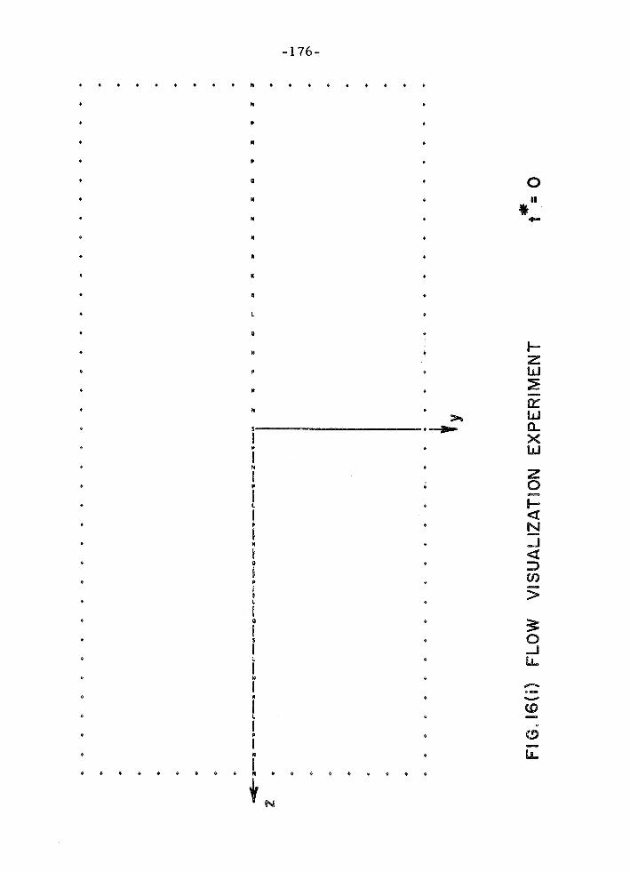
G. Background for the Momentum Transfer Experiments

Pr io r to time zero, fluid flows in the x direction at a speed

Uo(y). At time zero a random area-impulse independent of x i s ap-

plied in the x , z plane to generate a row of line vortices. The initial

random velocity component in the x direction is zero. The motion of

the line vortices in the y, z plane is independent of the x momentum

they transport. The flow visualization experiments of subsection F

show how the vortices disperse, but give no indication of how rapidly

the flow they induce distorts the mean speed profile U(y,t). If the

flow were studied in a physical experiment, U(y,t) would be found by

taking a hot-wire t raverse along z a t height y and t ime t. UQy, t )

would be the average x speed measured, A t raverse over many eddy

correlation lengths can be regarded a s a sequence of measurements

over an ensemble of independent experiments. This suggests the

model experiment used here to define U(y, t) formally, Call i t

Experiment 1 . N

The experiment i s performed at t ime t , Let p(u Iy)du be the proba-

bility that the speed a t height y and random z l ies between u and

u f du (u i s taken to be total velocity in the x direction here) , Then

the mean speed profile U(y) i s defined by

Since x speed i s conserved (equation 35) and the velocity fluctuations

in the x direction a r e initially zero, the measured speed u i s uniquely

related to the original height y of the fluid column the measuring o

instrument intercepts:

If Uo(yo) i s monotonic (like U = S2yo), then the inverse relation 0

i s unique. Let p(yo ly)dyo be the probability that the fluid column

intercepted at y originated between y and y + dye. Then 0 0

Differentiate with respect to u:

N dY 0 p(u ly) = p(Y0(u) ly) 0

Then

Substitute u = U (y ) : 0 0

Equation 79 i s the definition of U(y) in t e r m s of the transition prob-

ability p( y 1 y). 0

The trouble with Experiment l i s that i t cannot be performed

on a computer. The only way to find yo for a fluid column selected

a t specs ied y, t and random z i s to r eve r s e the calculation and

c a r r y the designated column back to i t s original location, That i s

-184-

impossible in practice, because the computer solution i s inherently

unstable. E r r o r drift (not to mention vortex capture) makes the flow

irreversible and sustained, detailed backtracking impossible. An

experiment that can be performed i s

Experiment 2.

At time zero place a tes t particle a t random inside a large a r ea A o

straddling the vortex row:

If P(yo9 zo)dyodzo is the probability that the particle originates be - tween y and y +dyo9 zo and z +dr , then

0 0 o 0

(HLI-' (yo. 2,) &Ao

P(y09 zo) =

0 otherwise,

By time t , the converted boundary of the a r ea i s distorted:

-185-

The probability density for the cur ren t part icle location i s

P(y , z ) = P(y, 1 (y9 z)E A) P((YY z)EA)

where

P(y , z I (y, z)EA) = the probability density a t (y, z ) given that

(y, z ) l i e s inside the convected boundary

of A ,

P((Y, z)&A) = the probability that (y, z ) l i e s inside A.

By incompressibility

If the h0rizonta.l boundaries distort a distance l e s s than h and the

vert ical boundaries distort a distance l e s s than 8 ,

E - L + 1 < z < - - 1 9 P( (y , z)cA) = I for 2 2

H - H + h < y < - - h . 2 2

and P((y , z)EA) drops rapidly to ze ro outside that a r ea , If h<< H

and I << k,

almost everywhere inside the original a r e a spanned by A . Thus y o

and z a r e independent, and sampling only those part icles which hap-

pen to a r r i ve at y at t ime t does not bias the distribution over z ,

-186-

Let P(yo l y ) dy be the conditional probability that the test particle 0

was originally located between y and y t dyo given that it has 0 0

arr ived at y. Then

and sampling only those particles which a r r ive at y in Experiment

2 is equivalent to sampling at height y and random z in Experiment

1, From the definition of U(y),

U(Y) = 'J Uo(yo) P (y 0 Id dye 0

Equation 81 i s not usable a s i t stands, because a digital

computer cannot handle continuous functions, Suppose the region

- ~ / 2 G y d ~ / 2 is broken into horizontal bands k with center

height yk and band height %:

Define the average speed in band ko

where the integration i s ca r r ied from y -6 / 2 to y k t 6 k / ~ . From k k

equation 8 1,

This equation could be written

exactly for any k i f the stack of bands extended to y -ti- m. But the

computer can deal with a finite stack only. When k is summed over 0

a finite sequence of ba.nds, the equation st i l l holds if band k i s not

too close to the top o r bottom of the stack, F o r yocko and ysk,

P (yo ly) i s then zero for the bands that fall outside the sum. If

U (y ) does not change too rapidly in band k , 0 0 0

where

The double integral in brackets can be identified a s follows.

The probability that the part icle occupies band k at t ime t i s

f rom equation $8. Let P(k , k) be the probability that the test part i - 0

cle originated in band ko - and occupies band k a t t ime t , that i s ,

-188-

where P(y ,y)dy dy i s the probability that the particle started be- 0 0

tween y and y t dyo and currently l ies between y and y + dy. But 0 0

From equation 83,

Thus the bracketed factor in equation $ 2 is the band-transition prob-

ability P(ko Ik), the probability that the particle originated in band

k given that it occupies band k a t t ime t. Equation 82 becomes 0

when band k is deep enough in the stack of bands that fluid originating

outside of the bands summed in equation 85 rare ly enters k, Equa-

tion 85 i s the discrete analog of equation 81.

The transition probabilities P(ko lk) could be found by car ry-

ing one test particle per run (Experiment 21, but that would be

absurdly wasteful, The numerical Monte Carlo experiments were

run according to

Experiment 3.

Each horizontal band i s separated into cel ls a s shown in figure 17.

At time zero a tes t particle i s placed a t random in each cell (a con-

ventional random number subroutine i s used). Pf the cell. a rea in

band ko i s a(ko), then the number density of tes t particles convected

f rom band ko i s p(k ) = a- ' (k ) At t ime t a survey i s made of the 0 0

tes t particles currently in each band k. If n(ko,k) of them originated

in k (transitions like c + d in figure 17 a r e summed with transitions 0

like a +b ) , then an unbiased estimator of P(ko Ik) i s

Notice B pe(ko 1 k) = 1 regardless of how untypical the particular ko

experimental results happen to be. The Monte Carlo estimate for

the mean speed U(y ) at yk. t i s k

for k not too close to the top o r bottom bands. In practice that r e -

striction meant that U(k) could not be estimated in the top or bottom

bands of figure 17, but could be estimated in the second to the top

o r bottom bands. Since transitions c +- d a r e summed with transi-

e e tions a + b 9 U (yk) = -f U (-yk) if Uo(yko) = + Uo(-yko) Thus five

independent speeds a r e obtained from the twelve band setup of figure

e The estimate 'U (k) i s refined by running the experiment many

t imes and averaging the results , Placing tes t particles in cel ls ,

grading p fo r maximum particle density near the vort ices, and sum-

ming a + b and c +-d transitions help to minimize the variance of the

estimate for small times. If the particles were scattered a t random

in each band, the clustering characteristic of random distributions

would occur. When the particles a r e placed a t random in band cells

instead, the density over a band i s stil l uniform and the clustering

i s eliminated. The particles remain spaced apar t until the turbulent

motion itself scrambles them into a random distribution. Grading p

puts the most particles where the most action is - near the vortices.

Summing transitions like a + b and c -F d exploits continuity to cancel

untypical results. If a particular se t of vortices causes unusually

many a + b transitions, then c + d transitions a r e unusually inhibited.

La te r , when the a r r a y of figure 17 i s thoroughly mixed, none of

these devices works.

Suppose the initial speed difference between bands k and ko i s

F rom equation 85,

U (k) = [U (k) + ~ ( k , k)] P(k I k) = uo(k) + 6U (k) , 0 0 0

where the speed change between times 0 and t i s

and the fact that 22 P(ko lk) = 1 has been used. The estimated speed ko

change i s

A good estimate of the speed change is required. The square e r r o r

of the estimate i s

Once the mixing i s thorough, the estimates pe(kbJk) and P(koIk)

should be nearly independent for kb ko (they cannot be strictly

e independent, since X P (k ik) = 1; however A(ko, ko) = 0, so some

ko 0

of the slack is taken bp by the t e rms with kb or ko = k which have

zero coefficients anyway). Then the mean square e r r o r for one

experiment i s

Suppose p ( b ) = constant (the analysis for non-constant p is very

complicated). Then

where T(k) i s the total number of tes t particles in band k at time t ,

T ( k ) = x n ( k o , k )

k 0

F o r the t ime being, the arguments (k k), (ko lk), (k) a r e dropped. o

Define a random variable a a such that for every point a in band k ,

1-P, if a came from k * o9 a = a

-P , if not .

Since Pe = n / ~ ,

a i s independent of T , since the origin of a particular particle can- a

not be biased by the total number of particles in the band if p(k ) = 0

constant. Thus

where ( ) i s an average over 7". But

and if the mixing has been sufficiently thorough that the particle his-

tories a r e almost independent.

Thus

e for large T. The mean square e r r o r in 6U (k) i s

2 for thorough mixing. A (k) i s the mean square deviation of the speed

in band k from the original speed U (k). If Q experiments a r e run, 0

the root mean square e r r o r divided by the speed change to be meas-

ured is

That ratio must be small for the results to be meaningful. The ex-

periments of subsection H show that h i s much la rger than bU, that

i s , the vortices transport x momentum rapidly, but the net transport

i s rather small. The number of experiments Q and the number of

points per band T in each experiment must be Barge, and the Monte

Carlo technique is barely feasible after the tes t particles a r e thor-

oughly mixed.

H. Momentum Transfer Experiments

The momentum transfer program begins an experiment by

computing vortex strengths from random phase input data, and by

locating test particles in cells of a specified matrix using pseudo-

random numbers generated internally, Once the initial conditions

a r e se t , the momentum transfer program solves about the same

mechanical problem a s the flow visualization program. Lengths,

t imes and vortex strengths a r e non-dimensionalized the same way.

A vortex i s convected in the field induced by the other vort ices; a

tes t particle i s convected in the field of a l l the vort ices. The cap-

ture cr i te r ion t r ea t s tes t part icles like vort ices of z e ro strength.

A tes t particle i s not annihilated when i t i s captured - it r ides i t s

captor vortex. If that vortex is captured in turn, the t e s t particle

passes to the new captor. The number of vort ices drops every

t ime a vortex i s captured, but tes t part icles a r e conserved. The

t es t part icles a r e surveyed periodically to find the icurrent band-

t ransfer data n(ko,k). After the experiment has been run with f resh

random phases and pseudo-random numbers a s many t imes a s de-

s i r ed , the accumuPated data a r e passed through two data reduction

programs.

The f i r s t program sums the n(ko,k) for each survey over

al l the experiments and computes est imates of %'he band-transition

probabilities P(ko Ik) by equation 86. The P(ko Ik) a r e related to a

step-function approximation of the continuous transition probability

P(yo 1 y). Define

P(k lk) 0

g(yo9y) = for y E YE;BC 6ko

o ko9

The expression 'yck' means y l i e s in band k, i. e. , ( y k - 6 k / ~ ) _< y

< (yk 4- bk/2). F r o m equation 84,

so g(yo,y) i s constant over the rectangle y r k yrk and equals the 0 0'

average value of P(yo l y ) there. Plots of g(yo, y) show the probability

distribution for original heights yo spreading away from the current

height y&. Using data from al l the experiments, the f i r s t data

reduction program gives estimates pe(k lk) f rom which plots of 0

e g (yz, y*) can be made.

The second data reduction program computes transition prob-

abilities, speeds and speed changes for each experiment using equa-

tions 86 and 87. If the initial speed profile i s l inear , U = Qy, then 0

the original vortex spacing X i s still the only length in the problem,

and U i s non-dimensionalized on &?A:

U u;': = - a%. '

The program averages the speed change estimates 6 ~ " ~ ( k ) over al l

the experiments and computes empirical standard e r r o r s

where Q i s the number of experiments,

Figures 18 and l 9 show the results of the f i r s t and second data

reduction programs for nine experiments run with the same values of

T * , o9 N , R ( 1 ) , T:k and F used to produce figures 16. T':% i s the time

between tes t particle surveys, and F i s the number of surveys. The

cell matrix, with 12 bands and 180 cells, i s shown in figure 17. The

band center locations y:R band heights 6* and tes t particle densities k ' k

p*(k) for the upper half of the matrix a r e a s follows:

BAND Y :k 6 96 P :k

1 7.1 1.8 .2778

2 5.4 1 .6 .3750

3 3.9 1 .4 .5000

4 2.6 1 .2 .6667

5 1.5 1.0 .9000

6 . 5 1.0 1.0000 .

The upper and lower halves of the matr ix a r e symqe t r i c a l a s shown.

The non-dimensional length and height of the mat r ix a r e

Both a r e large compared with the distance the boundary is distorted

up to t:k = 5. The original row of 45 vort ices extends 1 2 units beyond

the vert ical boundaries of the matr ix. The transition probability

est imates should be nearly the same a s they would be if the tes t par-

t icles moved in a field t ruly homogeneous in z.

e Figure 18 (i) shows g (y::, JT*) for y::~ 2 plotted against y:k a t

0 0

t imes t::: = 0 , 1 , . . , ,5. Figures 18 (ii) and 18 (iii) show the same

sequence for yS%4 and y S ~ 4 . At t::: = S p the probability distribution

over y':: given y ~ 2 i s s t i l l sharply peaked in band 2. The distribution 0

i s much more diffuse f o r y ~ 4 ~ and fo r y ~ 6 , the probability has spread

almost uniformly over the band occupied by the vort ices (cf . figures

16). F igures 19 show the speed change est imates for an

initially l inear shear profile a t t imes t* = 0, , . . ,5 . Es t imates in

the top band a r e impossible, because fluid without tes t part icles

-197-

intrudes there; no points a t y:: = 7.1 a r e shown. The heavy dots

represent estimates averaged over the nine experiments, the ve r -

tical lines represent standard e r r o r s of the mean computed from

equation 88, and the shaded bands represent speed change profiles

a s nearly a s they can be specified. The oblique line d U * = -y*

corresponds to fully stopped flow. The nine experiments took 20

minutes on a n IBM 7094 computer.

No analytical theory can predict the curves of figures 19.

A comparison of figures 16 and 19 shows that the speed change max-

imum and strong vortex dipoles propagate into the shear flow to-

gether. The time scales for Reynolds s t r e s s generation and mean

flow change and for convection of turbulence in its own random

field a r e the same. The maximum speed change a t t*: = 5 is

- d U + - .4+. 5 in band 4. The original speed there i s U* = 2 4 3.2, 0

so the mean speed changes about 2070. The las t graph of figure l 8 (ii)

shows that the dispersion of the speed about its original value in band

4 is A*(4) - 2 a t t*< = 5. By t:: = 5, the speed range in band 4 is a s

large a s the mean speed there , yet the mean speed change i s small.

It i s surprising that flows a s inhomogenesus on y a s the flow in

figure 16 could mix fluid columns a s well a s figures 11 8 show with

such a small net transport of momentum.

Before the vortices have mixed the tes t particles thoroughly,

the use of cel ls , grading of p , and summing of transitions like a + b

and c + d in figure 17 keep down the standard e r r o r s in speed es t i -

mates. After thorough random mixsing s f the tes t particles, the

e r r o r s cannot be reduced below the prediction of equation 87. About

-198-

20 test particles occupied band 4, and 20 more occupied its comple-

ment, band 9. Since transitions a b and c -+d a r e summed, the

speed estimates in band 4 a r e based on ( T(4) ) - 40 particles per

experiment and Q = 9 experiments. The theoretical prediction of

the standard e r r o r after thorough mixing i s

from equation 87 (equation 87 was derived for p(k) = constant, but

it i s accurate enough for a crude estimate like this). The second

data reduction program computed the following empirical standard

e r rors :

By t::: = 4, the fluid in band 4 i s mixed well enough for equation 87

to be valid. As A+: grows with t ime, the accuracy of a mean speed

e stimate drops, Since the vortices mix fluid columns thoroughly

without having much effect on the mean flow, the expected e r r o r of

a speed change estimate grows more rapidly than the speed change

itself. The Monte Carlo method is time limited for practical pur-

poses. There i s no point in carrying the experiments much beyond

t* = 5-

FIG. 89 (i) SPEED CHANGE PROFILE

FIG. 19 (ii) SPEED CHANGE PROFILE

FIG, 19 ( i i i 1 SPEED CHANGE PROF1 kE

6. Summary

This chapter began with the assumption that the propagation

of turbulence through a rapidly shearing flow depends pr imar i ly on

random stretching of mean field vorticity. Reynolds s t r e s s was taken

a s the mechanical signature of random vorticity in a shear flow.

Rapid shearing means ff << d., where I! i s a fluctuation speed, L i s

an eddy s ize , and 52 i s a typical mean vorticity. The equations of

turbulent motion were linearized under the assumption I!/<< 52L, and

the history of the Reynolds s t r e s s a (y , t ) acting on a mean flow

U(y) = 52y in the x direction was studied. The original random vor -

ticity was assumed to be generated a t t h e ze ro by impulses homo-

geneous in x , z and concentrated near y = 0. Turbulence near y = 0

was expected to catalyze the growth of random vorticity further out

by stretching mean vorticity so that the turbulence would grow stead-

ily more intense and propagate further and further through the mean

flow. But the Reynolds s t r e s s was found to re lax into a steady dis -

tribution a s Qt 300. AS f a r a s the Reynolds s t r e s s i s a measure of

turbulent intensity, random stretching of mean vorticity alone cannot

yield steadily propagating turbulence.

The problem was simplified next by assuming that a l l flow

propert ies a r e independent s f x. In that case , the eddy motion in

the y , z plane i s independent of the x momentum i t t ranspor ts , and

the mean speed U(y, t ) i s diffused like a passive scalar . The equa-

tions of motion were partially linearized by neglecting convection of

eddies in the y , z plane, and wave equations for o (y , t ) and U(y, t) were

derived. The solutions a r e worthless , however, fo r t imes t'>L/I/.

-207-

Turbulence artificially steady in the y , z plane exer ts a steady grip

on the mean flow and forces U to become independent of y over a

l a rger and larger interval -Y(t)< y < Y (t). In a real flow the eddies

disperse a s fast a s U diffuses. The core of the problem was found

to be convection of eddies in their own random field.

The chapter ended with numerical turbulence experiments

designed to find how quickly concentrated vortex columns parallel

to x disperse over the y, z plane under their own induction, and how

effectively they diffuse U(y,t). The ra te of e r r o r accumulation was

analyzed carefully. The mean square e r r o r of the computed location

of a vortex was found to diverge exponentially with time according

to a generalized random walk equation. Detailed vortex Potations

a r e unimportant in a turbulence experiment; compqted trajectories

must not diverge too rapidly from current physical t rajectories, but

the accumulated displacements of computed locations from actual

locations can be large. It was shown, however, that unless a lower

limit on the distance between any two vortices i s imposed, the

velocity of e r r o r drift can dominate the flow velocity no matter

how small a time increment is used in the computations. Vortices

which approach each other closely must be united. Uniting vortices

during the computations was justified by finding a capture c ross

section for the interaction of two vortices in a strain field. Numeri-

cal flow visualization and momentum transfer experiments confirmed

the result that columnar eddies disperse a s fast a s they transport

momentum. In case the flow properties a r e independent of x , the

t ime scales for non-linear convection and turbulence propagation

a r e the same, and no analytical solution for the propagation is pos -

sible. That does not mean that the time scales for propagation and

non-linear convection a r e the same in more real ist ic situations

where turbulent quantities depend on x. The t ime scale for the

propagation of random vorticity of strength b/L through a field

- 1 of mean vorticity 52 i s not a s short a s 52 , a s originally expected,

but it may not be a s long a s L 10. Weak interaction among turbu-

lent eddies may f ree the Reynolds s t r e s s , steady for t>> $2-I under

the linear approxirn ation, and allow i ts gradual diffusion,

REFERENCES

1. C o r r s i n , S. , and Kis t l e r , A. L. , "The F r e e - S t r e a m Boundaries

of Turbulent F lows, " NACA Tech. Note No. 31 33 (1 954).

2. Saffman, P. G. , "The Motion of Turbulent Slugs along P ipes , "

J P L Space P r o g r a m s Summary 37-22, Vol. 4 (1965).

3. Coles , D . , "Interfaces and Intermit tency in Turbulent Shear

Flow, " Mechanique de l a Turbulence, Editions du Cent re

Nationale de l a Recherche Scientifique, Paris (1 962),

pp. 224-250.

4. Phi l l ips , 8. M. , he Irrotat ional Motion outs jde a F r e e Turbu-

lent Bqundary, I' P r o c . Cam. Phil . Soc. , Vol. 51 (1 955),

pp. 220-229.

5. Moffatt, H. Me, "The Interaction of Turbulence with Rapid Uni-

f o r m Shea r , " SUDAER No. 242, Stanford University (1 965).

6. Lighthill, M. J . , F o u r i e r Analysis and Generalized Funct ions,

Cambridge (Eng. ) University P r e s s (4.962).

7. Dwight, M. B. , Tables of Integrals and Other Mathematical

Data, 4th Ed. , The Macmillan Company, New York (1961). - - 8, Townsend, A. A . , The St ruc ture of Turbulent Shear Flows,

Cambridge (Eng. ) University P r e s s (1956), pp. 206-21 (9.

9. F a v r e , A s , Caviglio, J . , and Dumas, R . , "Correlat ions

Spatio -Tempore l les e n Ecoulements Turbulents , " Mechanique

de la Turbulence, Editions du Cent re Nationale de l a We-

cherche Scientic, Paris (1 962), pp, 41 9-445.

10, Lamb, Pi. , Hydrodynamics, 6th - Ed, , Dover PubBications, New

York (1932).

-210-

11. Abernathy, F. H . , and Kronauer, R . E, , he Formation of

Vortex S t ree t s , I' Journal of Fluid Mechanics; Vol. 13 (1962),

pp. 1-20.

12. Brillouin, L. , Science and Information Theory, 2nd Ed. , Aca- -

demic P r e s s Inc. , New York (1962), pp. 78-79.

13. Batchelor, C. K. , The Theory of Homogeneous Turbulence,

Cambridge (Eng. ) University P r e s s (1 960), pp. 186- 187.

14. Onsager , E. , "Statistical Hydrodynamics, I' Nuovo Cimento,

Supplement, Vol. 6 (19491, pp. 279-2820

APPENDIX A

Evaluation of L.. (k, k ) 1J 02

The equation to be integrated i s

where

2 2 2 2 and k , k a r e fixed. k is kl t k2 + k3, and kl ,kg will often appear 1 3

2 2 2 in the combination kl + k3 = 1 . Thus

and by the initial condition, L21 = 0. Then

so L1 = 1 . It can likewise be shown that L31. L1 3, Lz3 = 0 and Lg3 =

1. L22 satisfies

Integration and use of the initial condition L (k k ) = % gives 22 02' 02 2 2 2

L22 = k:/kZ9 where ko = I + koZ. Then L I Z satisfies

and since L12(ko2, koz) = 0,

where

f 0 - 1 x tan $ - ) - - 2 2- l 2 (1 tx )

- 1 1 - 1 1 [ e l = tan (-) - tan - 0 St3 ST , k2 k02

k2

02

and

In the same way it can be shown that

-213-

APPENDIX B

Evaluation of the S t ress Integrals in the Vortex Sheet Problem

From equations 27,

where

But

O(kl.k3) i(ko2fkb2)y

2 e dkb2kdo2dkldk3 . (Bl)

n

From equations 21,

and since 8 i s the Fourier transform of a rea l function symmetric

with respect to changes in sign of i ts arguments,

Reversing the signs of kl and k and switching the ro les of ko2 and 3

kb2 a l t e r s the right hand side of B1 by a change of sign only, s o

The integral over kb2 in I2 may be ca r r i ed out a s follows:

- e dkb2 - dk'

02 -a -00

f rom Dwight [ 7 ] , p. 224. The integral over ko2 i s

where

f rom the definitions below equation B 5. Substitute

K can be regarded a s a function of 5 satisfying

since the integration i s the same as that which led to 432. Thus

From equations B2 and B 3 ,

The symmetry property of O was used twice. Since o = I +( +I )= IZ. 2 5 3

equation 28 in the text has been verified.

-216-

APPENDIX C

Proof that Eauation 31 i s Valid in the Limit a t +oo

The t e r m s dropped from equation 31, analogous to I1 and I3

in the vortex sheet problem, a r e

Under transformations 32 and 33, these become

Both integrals converge for large 8 even when the limit %1$ +GO i s

taken before the integrations a r e performed explicitly. Thus a s

Stt +co,

Thus J1 is 0($2t)-' and J g i s O(&?tleL a s &?t - roo . It may seem incon-

sistent that these integrals cancel in the vortex skeet problem when

they appear to be of different o rders of magnitude in the limit Stt+a3.

The answer i s that in that special ease AO ( P ' l , 0 9 p 2 , 1 ) is ze ro , and 2 1

Ai l i s itself ~ ( S t t ) - ' under transformations 32 and 33.

APPENDIX D

Singular Perturbation Solution for s (q , T ) , r ( q , T )

The object i s to solve equations 45, 46, 47 for a l l q and r N

It i s reasonable to use an expanded time coordinate T = T/€ and to t ry N N

to find asymptotic ser ies expansions of s (q , T;€ ) and r ( r l , r; E ). The

wave equations 45 a r e

in t e rms of the expanded coordinate, and equations 46 and 47 a r e un-

changed. Expand s and r a s follows:

The initial conditions of equations 47 a r e

When coefficients of separate powers of C a r e se t equal to zero in

the expansions of equations DB, the following system results:

The equations have been solved step-by-step using the expanded

initial conditions. Thus the power se r ies for s and r begin

equations 48 in the text. The ordering breaks down near n - E , and CV

i t i s necessary to use an expanded space coordinate 7 = q / ~ . The

wave equations become

sketch, and i t s expansion around / r, = 0 begins 'l

CY C* N m,

The ' inner' expansions of s (q , T;€) and r (q , T;E) begin

w N lu '-4 2 - - s = S o ( ? . ~ ) + ~ S ~ ( r l . r ) + B S2(q.-r) + e v e .

N N N m 2 " " r = Ro(q , r ) + tR1(q9r) + E R2(qI T) + . .. .

The expanded initial conditions rare

W (V (Zs

R (;,o) = 0s R1(;yO) = '1, RZ(q90) = R3(q90) = s e e = 0 y 0

IU N

S0(q90) = S1(q.O) = . * . = 0.

The dependent variables r and s have been expanded in two fo rms

suitable for ' inner ' and 'outer ' intervals of q ,

N N N N

( inner) a = Ao(q , r ) f eA1(q,r) f ... , w N

(outer) a = a ( q , ~ ) + e a l ( q , r ) + - 0 - , 0

where a represents ei ther r o r s . The matching conditions between

such expansions a r e

N N N

Lim Ao(q, r) = ao(O. r) , l{l+m

Thus, f rom the outer solutions 48 and the expansion fo r g ,

k i m S = 0 9 0

1; l+m

k The coefficients of E" and E in the expansions of 132 a r e

The solutions a r e

2 from the expanded initial and matching conditions. The O(E ) set

of equations i s finally

These equations contain the rn ean field approximation correction to

the linear results , The equations can be solved by the method of

characterist ics, Some geometrica,B quantities are shown in the

sketch:

Substitute

By adding and subtracting the transformed wave equations, the equa-

t ions for the evolution of R2 t S 2 and R 2 - S2 along the characteris-

t ic s specified by u and v a r e obtained:

Thus

N '-4

u and v switch signs in the four regions A , B, C , D of the q - T diagram,

so the integrations must be carr ied out separately in each region.

In region A, for example, u > 0, v > 0 , and the absolute value signs

i n the integrals can be ignored, The result is

In region @, u > 8, v < O 9 but utv > 0. Thus the quantity vf x switches

sign as x i s integrated from v to uc The result i s

The results in regions C and D can be found immediately from the

sylinmetry of s 'and antisymmetry of r on q , Thus the inner expan-

sions begin

H ff

in regions A and D outside of the characterist ics leaving (q, T) = ( 0 , 0 ) ,

and

in regions B and C between those characterist ics, Equations D3 a r e m

the limit of equations 48 for q = r q - E. Thus equations 48 a r e the (V N

correct expansions wherever r) > -re F o r q < T, o r r] < T, equations

49 a r e valid and represent the effect of mean flow distortion lost in

the linear approximation.

-224-

APPENDIX E

Derivation of T(4) and +(y, 0) for the Steady Vortex Street

Complex variables with the sign conventions of Lamb [ lo] a r e

used. Thus the location y , z i s assigned a complex number Z = zt iy ,

and and \CI a r e written a s a complex potential W = Q, t i+. The com-

plex potential for an infinite row of vortices of strength k located at

z = 0, - t B , 2 2B,... i s

ik nZ W = - log sin , 2n

from Lamb. The potential for the vortices of alternating sign spaced

X apar t i s then

w=- nZ i k log sin - - - nZ log sin '(Z-h) = ik log (-tan 211- ZX 271- 2h 2n

Thus

In particular

k si."

C(y9 0) = log 1 t cash

9

which is the second of equations 51 in the text. The complex velocity

is

d W - w-iv = - - - ik/4X dZ nZ nZ

sin z c o s

The expression for W(Z) can be inverted to give

and the complex velocity can be written a s a function of W:

- ik w-iv = - 2aW 2 h

cos - k

The square of the speed i s

Thus

k2 aW ::: v 2 = - 2aW cos -

4X 2 COS - k k

k 2 - - - cos - 27T ( w ~ w * ) + cos -i; E a (W-W*

k 9

8h2

from Dwight [ 7 ] , p. 79. h t e r m s of QP and +, 2 kZ v (QP,+) = - cos

8h2

The orbi t t ime T($) is then

f rom equation 50 of the text, where

a = cosh * > l e k

F r o m Dwight, p, 105,

Again from Dwight, p. 152, Z lsinh x cosh x l = fx , and

which i s the f i r s t of equations 51 in the text.

APPENDIX F n

Derivation of the Mean Square E r r o r Velocity $ "E ,

-

Write the convective part of the acceleration

Then v = - Ta / 2 , Equation 68 is c -'C

F rom the definitions of q G i 9 r i'

where

Similarly

where (i, j ; q ) i s the same a s ( i , j;5) except that t he roles of q and 5

a r e reversed. Thus

If the vortices a r e distributed symmetrically around y, z , then a = 0. -'C

If the location of each vortex i s independent of i ts strength,

- k.k.k k

-' c i j m n 64s i j m n r . r . r r

i j m n

If k. and k. a r e independent for i # j , 1 J

Thus

From the definition of the brackets,

Thus

If the vortices a r e distributed isotropically around y, z , then quan-

4 4 t i t ies like ~ . 5 . / r . r a r e zero unless i = j, and

1~ n j

- 2 2 = r a /4, equation 70 in the text follows immediately. "C

APPENDIX G

Motion of the Center of a Continuous Vorticity

Distribution in a Uniform Translation and Strain Field

The speed of the center of vorticity in the y direction i s

since vorticity i s conserved. But

where the varticity convection equation and continuity equation were

used. If the vorticity 5 goes to zero sufficiently fast toward infinity,

a Y py (v5) dydz = - v6 dydz

Thus

Since the velocity field consists of a uniform translation plus a

s train plus the velocity induced by the vorticity distribution 6,

where r 2 = ( Y - ~ ' ) ~ + ( z - z ' ) ~ . Then

The las t integral i s zero since it switches sign when the dummy var-

iables y and y' a r e exchanged. Division by . f $ d ~ gives

? = v + ~ Y .

e

The equation Z = W - cuZ follows from a similar argument.