The Specialist Committee on Uncertainty Analysis

Proceedings of 26th ITTC – Volume I

299

The Specialist Committee on Uncertainty Analysis

Final Report and Recommendations to the 26th ITTC

1. INTRODUCTION

1.1 Membership and Meetings

The Uncertainty Analysis Committee (UAC) was appointed by the 25th ITTC in Fukuoka, Japan, 2008, and it consists of the following members (see picture in Figure 1): Mr. Baoshan Wu: China Ship Scientific

Research Centre, CSSRC, Wuxi, Jiangsu, China.

Dr. Michael D. Woodward: School of

Marine Science & Technology, Newcastle University, Newcastle-upon-Tyne, UK.

Dr. Shigeru Nishio: Kobe University,

Faculty of Maritime Sciences, Department of Maritime Safety Management, Kobe, Japan.

Mr. Angelo Olivieri: The Italian Ship

Model Basin, INSEAN, Via di Vallerano, Roma, Italy

Dr. Luis Pérez Rojas: Universidad

Politécnica De Madrid, Escuela Técnica Superior De Ingenieros Navales, Spain.

Mr. Martijn van Rijsbergen: The

Maritime Research Institute Netherlands, MARIN, The Netherlands.

Dr. Ahmed Derradji-Aouat (Chairman):

National Research Council Canada, Institute for Ocean Technology, NRC-IOT, Newfoundland & Labrador, Canada.

In the picture (Figure 1), Dr. Joel T. Park, Naval Surface Warfare Center Carderock Division, Maryland, USA, participated in two meetings as an ex officio member. He was the chairman of the 25th ITTC UAC.

Three (3) UAC committee meetings were held. The host laboratories and times of the meetings were: Spain, Madrid University, January

2009 Italy, INSEAN, December 2009. Canada, NRC-IOT, June 2010.

During the last year of the 26th ITTC term, several members of the UAC were sick. However, this problem was mitigated and managed relatively well; the committee faced only minor difficulties in achieving its mandated target.


300

Figure 1: The 26th ITTC Uncertainty Analysis Committee (ITTC - UAC) Left to right: Mr. Baoshan Wu, Dr. Luis Pérez Rojas, Dr. Joel Park, Dr. Angelo Olivieri, Mr. Martijn van Rijsbergen, Dr. Ahmed Derradji-Aouat, Dr. Michael D. Woodward, and Dr. Shigeru Nishio.

2. TERMS OF REFERENCE

In its Terms of Reference (ToR) document, the 26th ITTC mandated the UAC to perform the following Tasks: Monitor new developments in

verification & validation methodology and procedures.

Evaluate the state-of-the-art for evaluation

of uncertainty and determine if any methods have evolved that better represent what the ITTC community is using for practical CFD computations.

Update the ITTC recommended procedure

7.5-03-01-01 “Uncertainty Analysis in CFD, Uncertainty Assessment Methodology and Procedures” to take into account the revisions proposed by the Resistance Committee of the 25th ITTC.

Update the ITTC Recommended

Procedure 7.5-02-01-03, “Density and Viscosity of Water”.

a. Revise the formulae recommended by the ITTC, for the density, viscosity, and vapour pressure of water.

b. Develop uncertainty expressions for

these equations. c. Review existing procedures and

propose changes to ensure consistent use of this information.

Write an ITTC recommended procedure:

“Uncertainty Analysis for the 1978 ITTC Powering Prediction Method”, including a realistic example. Liaise with the Propulsion Committee.

Complete the revision of Procedures 7.5-

02-03-01.2 “Uncertainty Analysis Example for Propulsion test” and 7.5-02-03-02.2 “Uncertainty Analysis Example for open water test”.

Work with other technical committees to

develop or revise procedures related to uncertainty analysis.

Support the committees that have the


301

task of harmonizing the ITTC Recommended Procedures that contain uncertainty analysis with the ISO approach. Coordinate the work and review proposed revisions

A review of ITTC recommended procedure 7.5-03-01-01 “Uncertainty Analysis in CFD” was conducted in light of the revisions proposed by the Resistance Committee of the 25th ITTC. After review and several discussions, the UAC reached the conclusion that Procedure 7.5-03-01-01 does not need to be updated. The procedure in itself is new (developed for the 25th ITTC, 2008), and no new information to add.

ITTC procedure 7.5-02-01-03, “Density and Viscosity of Water as completely overhauled. The procedure was updated and expanded to include the properties of both freshwater and seawater. In addition to density and viscosity, equations and uncertainties for vapour pressure are included. This updated and expanded procedure (7.5-02-01-03, Revision 02, 2011) was developed on the basis of the latest international standards on water properties.

Two ITTC procedures 7.5-02-03-01.2 “Uncertainty Analysis Example for Propulsion test” and 7.5-02-03-02.2 “Uncertainty Analysis Example for open water test” were revised, as per ISO-GUM (the procedure is presented in section 9). However, ITTC advisory committee (AC) modified its initial ToR and asked the Propulsion Committee to merge the two procedures1, and therefore the UAC recommendation to the 26th ITTC to accept the two procedures was withdrawn. In the minutes of the AC meeting # 3 (28th to 30th March, 2011, in Wien, Austria), the AC recommendation “Postpone publication because the procedure needs to be fully updated to the ISO standard” is not correct.

1 An email from the AC secretary to the UAC chair, dated April 5, 2011

2.1 Additional Activities

In addition, to the UAC organized a 2-day workshop on uncertainty analysis in St. John’s, NL, Canada. Members from all ITTC committees were invited to participate, and several handouts (2 CDs) were given. Some details are given in Appendix A.

The UAC, also, played a proactive role in interacting and discussing Uncertainty Analysis (UA) with other ITTC committees.

2.2 Uncertainty Analysis for ITTC

The 25th ITTC, Japan-2008, accepted a recommendation that ITTC uncertainty analyses procedures are to be developed as per the guidelines of the ISO (1995), also known as ISO-GUM (Guide to the Expression of Uncertainty in Measurements, JCGM, 2008a). International pressures for commerce and trade dictated that ITTC international tow tanks had to adopt international standards and follow the ISO-GUM guidelines. The 25th ITTC member organizations from geographic areas other than North America have demanded the use of ISO (1995) rather than AIAA (1999) or ASME (2005). Both AIAA and ASME are American organizations, and ISO was viewed as the legitimate international organization for guides and standards development.

Application of the ISO-GUM to experimental hydrodynamics is a fundamental shift in thinking and in assessing uncertainties from what the ITTC historically had followed. Up to the 24th ITTC in 2005, the ITTC opted for the method by the AIAA (1995), which was revised as AIAA (1999). AIAA standards are developed from wind tunnel experiments. And, those standards were imported to experimental hydrodynamics and tow tank testing.

As a consequence for adoption of the ISO (1995) guidelines two general and


302

fundamental UA procedures were developed. The first one is 7.5-02-01-01 “Guide to the Expression of Uncertainty in Experimental Hydrodynamics”. The second one is 7.5-01-03-01 “Uncertainty Analysis for Instrument Calibration”. Using these two procedures, task specific procedure (such as UA procedures for resistance and propulsion tests) can be easily developed. For example, the 25th ITTC developed UA procedures for PIV measurements on the basis of these two general procedures

2.3 Symbols and Definitions

The basic and general definitions for metrology terms used in this document are the same as those given by the International Vocabulary for Metrology (VIM, 2007, ISO publication from BIPM that is complimentary to the ISO-GUM, JCGM 2008,). Examples include definitions for terms such as “repeatability”, “reproducibility”, and many other terms and expressions regularly used in ISO (1995).

3. RECOMMENDATIONS AND PROPOSALS FOR FUTURE WORK

The only recommendation from the UAC is to accept the ITTC procedure 7.5-02-01-03, “Density and Viscosity of Water.

Two ITTC procedures 7.5-02-03-01.2 “Uncertainty Analysis Example for Propulsion test” and 7.5-02-03-02.2 “Uncertainty Analysis Example for open water test” were recommended, but then withdrawn. The ITTC-AC asked the Propulsion Committee to merge the two procedures as indicated above.

For future work, the UAC proposed a fundamental structural change to better benefit the ITTC. The UAC proposal for future work is given in Appendix B.

It should be noted that, in the minutes of the AC meeting # 3 (28th to 30th March, 2011, in Wien, Austria), the AC indicated that the UAC would discontinue the UAC for the 27th ITTC because the lack of deliverables is not correct. In fact, the recommendation made by the UAC (Appendix B) was accepted.

4. EXPERIMENTAL UNCERTAINTY ANALYSIS

4.1 History of UA

The modern history for the development of UA equations, rules, and guidelines was given by the 25th ITTC (2008a). In Appendix A of this report, a brief history is given for how the international organizations responsible for the administration and development for UA evolved. Together, both summaries provide an overall understanding for UA development from both the organizational and technical points of view

4.2 Fundamental Principles

The ISO-GUM methodology for the expression of UA in measurements are based on five (5) principles:

Principle # 1. The uncertainty results may be grouped in 2 categories called Type A uncertainty and Type B uncertainty. They are defined as follows: Type A uncertainties are those evaluated

by applying statistical methods to the results of a series of repeated measurements.

Type B uncertainties are those evaluated

by other means (other than the use of statistical methods).

Principle # 2. The components in type A uncertainty are defined by the estimated


303

variance, which includes the effect of the number of degrees of freedom (DOF).

Principle # 3. The components in type B uncertainty are also approximated by a corresponding variance, in which its existence is assumed.

Principle # 4. The combined uncertainty should be computed by the normal method for the combination of variances, now known as the law of propagation of uncertainty.

Principle # 5. For particular applications, the combined uncertainty should be multiplied by a coverage factor to obtain an overall uncertainty value. The overall uncertainty is now called expanded uncertainty. For the 95 % confidence level, the coverage factor is 2.

All necessary equations for general application of UA are given in the 25th ITTC (2008a).

5. WATER PROPERTIES: EQUATIONS AND UNCERTAINTY ANALYSIS

A procedure is recommended 7.5-02-01-03, Revision 02 (2011) “properties of water, both freshwater and seawater. The new procedure is generated from the latest international standards on water properties. The information included in this procedure is the density, viscosity, and vapour pressure as tables. The tables provide the sensitivity coefficients as a function of temperature so that the uncertainty in the property can be computed from the uncertainty in the water temperature measurement. Also, the tables include the uncertainty in the equations. Example uncertainty estimates are given in the procedure. References are provided so that other properties may be computed such as thermal conductivity, index of refraction, and surface tension.

The latest international standard on fresh water is IAPWS (2008a). The water properties, density, viscosity, and vapour pressure, were generated using Harvey, et al. (2008) computer program. The uncertainties in the freshwater properties are summarized in Table 1. An example result for freshwater density with its sensitivity coefficient is presented graphically in Figures 2 and 3.

A new international standard on seawater properties has been developed through the United Nations and several other international organizations. The standard for seawater properties is the International Thermodynamic Equations of Seawater (TEOS-10, 2010). The methodology is derived from IAWPS (2008b), and the associated computer code (IOC et al., 2010) calculates thermodynamic properties such as density and vapour pressure. Sharqawy et al. (2010) equations for viscosity and vapour pressure for seawater are adopted.

A significant characteristic in seawater properties is the salinity. For standard seawater, practical salinity has a value of 35 ppt, which corresponds to absolute salinity of 35.16504 ±0.007 g/kg using SI units. Uncertainty estimates in the seawater properties equations are listed in Table 2. Three-dimensional plots of density, viscosity, and vapour pressure are shown in Figures 4 through 7, where the absolute salinity of fresh water has a value of 0.0.

Table 1 Uncertainty in freshwater properties equations at the 95 % confidence limit.

Property Symbol U 95 UnitsDensity 1 ppmViscosity 1 %Vapour Pressure p v 0.02 %

Freshwater properties, 95% confidence

ppm = parts per million (0.0001 %)


304

Table 2 Uncertainty in seawater properties

equations at the 95 % confidence limit.

6. STATE OF THE ART REVIEW

A state of the art review was given in the 25th ITTC. Over the last 3 years, a number of significant developments have occurred. In particular, the ISO GUM 1995 is now the responsibility of the Joint Committee for Guides in Metrology (JCGM) within the Bureau Internaptional des Poids Mesures (BIPM), The JCGM web page is as follows: http://www.bipm.org/en/committees/jc/jcgm/.

The ISO GUM 1995 is now available on-line as JCGM (2008a), and the Vocabulary of International Metrology (VIM) as JCGM (2008b). In addition, JCGM is in the process of publishing seven supplements to JCGM (2008a). Two supplements have been published to date: JCGM (2008c) and JCGM (2009).

JCGM (2009) is an introduction to the ISO GUM 95, JCGM (2008a), and JCGM (2008c) describes the application of Monte Carlo methods to uncertainty estimates. For the present, Monte Carlo methods may be a useful research tool for the ITTC. However, ITTC procedures remain to be developed for routine applications. In the case of tow tank testing and experimental hydrodynamics, the usefulness of Monte Carlo methods has to be demonstrated, as an improvement or complementary in comparison to the

conventional methods outlined in the current ITTC procedure (2008a).

Figure 2: Freshwater and standard seawater density.

Figure 3: Sensitivity coefficients for freshwater and standard seawater density.

Verification and validation (V&V) has become an important issue within the computational community of ITTC. ASME (American Society of Engineers) has published a new standard for V&V as ASME (2009). Verification is to establish that the

Property Symbol U 95 UnitsDensity 8 ppmViscosity 1.5 %Vapour Pressure p v 0.1 %ppm = parts per million (0.0001 %)

Seawater properties, 95% confidence


305

code solves accurately the mathematical equations in the code while validation is the process that insures the mathematical model accurately portrays experimental data. ASME (2009) provides details of the V&V process (87 pages).

Figure 4: Seawater density.

This standard should be adopted by ITTC until it develops its own procedure. Additional details on V&V are discussed elsewhere in this report.

Figure 5: Seawater absolute viscosity.

The NIST (National Institute for Standards and Technology), the National Metrology Institute (NMI) for the USA has revised its guide on SI units by Thompson and Taylor (2008). It should be a useful reference document for ITTC.

Figure 6: Seawater kinematic viscosity

Figure 7: Seawater vapour pressure

The inter-laboratory comparison of surface ship model testing of two models should be completed by the 26th ITTC. Since that test program has been initiated, the uncertainty analysis procedures have been revised as ITTC (2008a) in conformance with the ISO GUM 1995, JCGM (2008a). The larger model of 5.720 m length was tested at the U. S. Navy David Taylor Model Basin (DTMB). The model tested was CEHIPAR Model 2716, which was manufactured by Canal de Experiencias Hidrodinámicas de El Pardo (CEHIPAR) in Madrid, Spain. The model is the same size and geometry as DTMB Model 5415. For that test, an uncertainty analysis was completed per ITTC (2008a). The results are reported in Park, et al. (2010a) with additional details in the report Park, et al. (2010b).


306

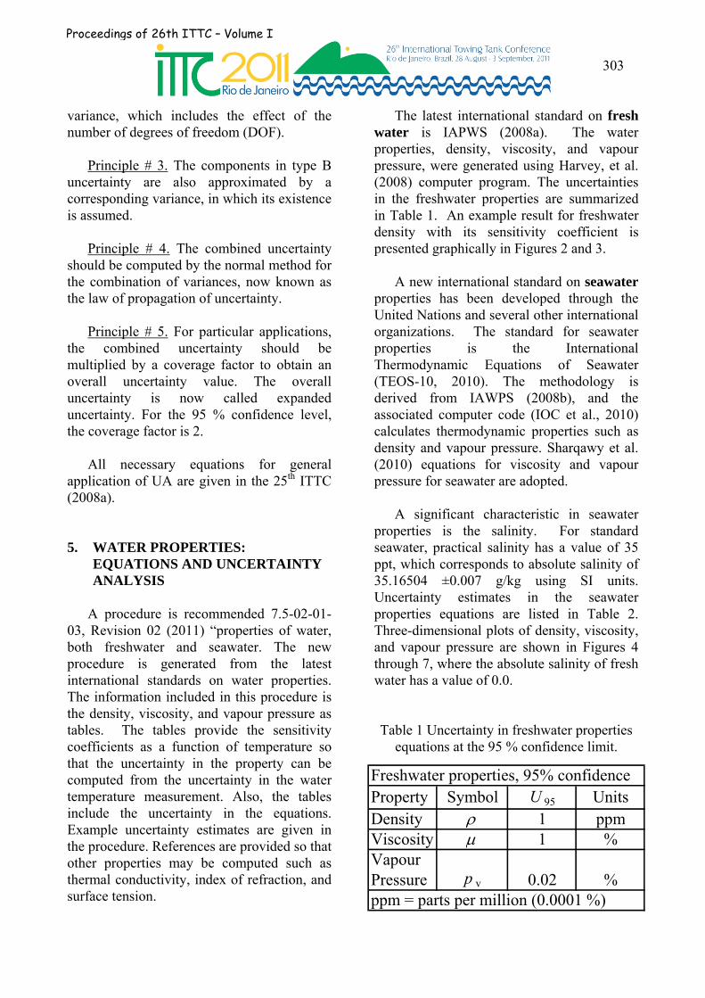
All data were acquired on a single day, and all instruments were calibrated with NIST traceability. Only the resistance results are reported here. Calibration uncertainty was derived by the methods in ITTC (2008b). Since the dominant term is the uncertainty estimate for the resistance measurement in the total resistance coefficient, only the calibration of the drag block gage is presented as an example in Figure 8.

The block gage was calibrated with NIST Class F weights with a tolerance of ±0.01 %. The error bars in the figure are from the NIST Class F weights while the dashed line is the uncertainty in the curve fit at the 95 % confidence limit. Force was corrected for local gravity and buoyancy per ITTC (2008b). As the figure indicates, a repeat calibration is in reasonable agreement with most data within the uncertainty of the curve fit.

The thermometer for the water properties computations had an uncertainty of ±0.10 °C. The water properties for the Reynolds number and the resistance coefficient were computed from Harvey, et al. (2008), which is the basis of the new ITTC water properties procedure.

Figure 8: Drag block gage calibration residuals

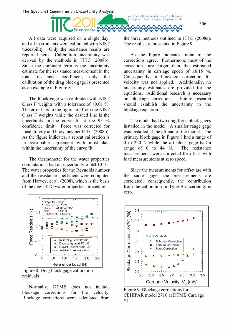
Normally, DTMB does not include blockage corrections for the velocity. Blockage corrections were calculated from

the three methods outlined in ITTC (2008c). The results are presented in Figure 9.

As the figure indicates, none of the corrections agree. Furthermore, most of the corrections are larger than the estimated uncertainty in carriage speed of ±0.15 %. Consequently, a blockage correction for velocity was not applied. Additionally, no uncertainty estimates are provided for the equations. Additional research is necessary on blockage corrections. Future research should establish the uncertainty in the blockage equation.

The model had two drag force block gages installed in the model. A smaller range gage was installed at the aft end of the model. The primary block gage in Figure 8 had a range of 0 to 220 N while the aft block gage had a range of 0 to 44 N. The resistance measurements were corrected for offset with load measurements at zero speed.

Since the measurements for offset are with the same gage, the measurements are correlated; consequently, the contribution from the calibration or Type B uncertainty is zero.

Carriage Velocity, Vu (m/s)

0.5 1.0 1.5 2.0 2.5 3.0 3.5

Blo

ckag

e C

orre

ctio

n,

V/V

u (%

)

0.0

0.1

0.2

0.3

0.4

0.5

0.6

Schuster CorrectionTamura CorrectionScott Correction

CEHIPAR 2716

Figure 9: Blockage corrections for CEHIPAR model 2716 at DTMB Carriage #1


307

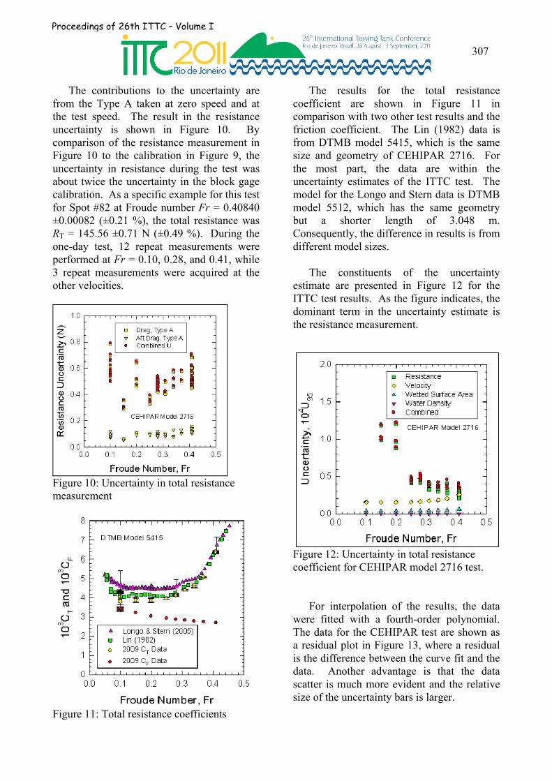
The contributions to the uncertainty are from the Type A taken at zero speed and at the test speed. The result in the resistance uncertainty is shown in Figure 10. By comparison of the resistance measurement in Figure 10 to the calibration in Figure 9, the uncertainty in resistance during the test was about twice the uncertainty in the block gage calibration. As a specific example for this test for Spot #82 at Froude number Fr = 0.40840 ±0.00082 (±0.21 %), the total resistance was RT = 145.56 ±0.71 N (±0.49 %). During the one-day test, 12 repeat measurements were performed at Fr = 0.10, 0.28, and 0.41, while 3 repeat measurements were acquired at the other velocities.

Figure 10: Uncertainty in total resistance measurement

Figure 11: Total resistance coefficients

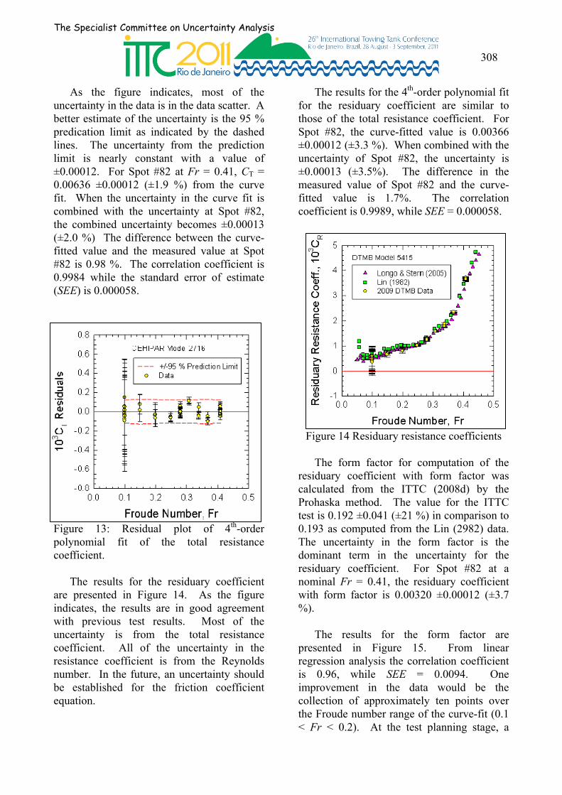
The results for the total resistance coefficient are shown in Figure 11 in comparison with two other test results and the friction coefficient. The Lin (1982) data is from DTMB model 5415, which is the same size and geometry of CEHIPAR 2716. For the most part, the data are within the uncertainty estimates of the ITTC test. The model for the Longo and Stern data is DTMB model 5512, which has the same geometry but a shorter length of 3.048 m. Consequently, the difference in results is from different model sizes.

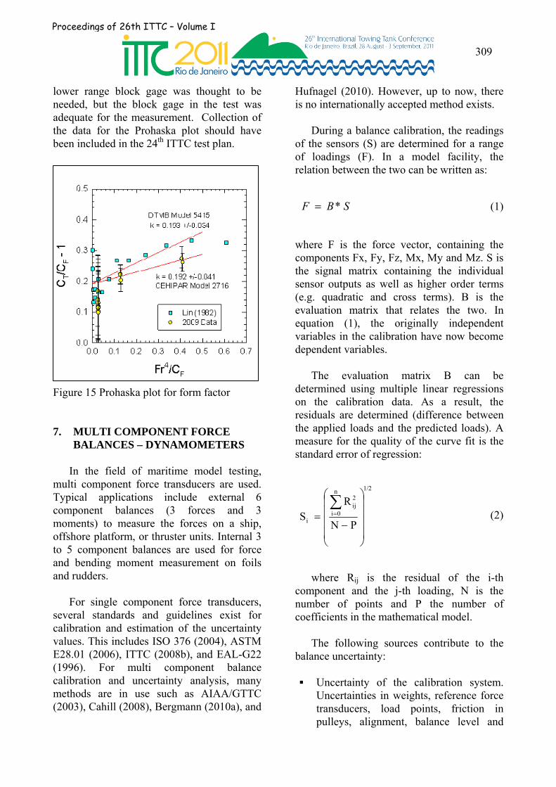
The constituents of the uncertainty estimate are presented in Figure 12 for the ITTC test results. As the figure indicates, the dominant term in the uncertainty estimate is the resistance measurement.

Figure 12: Uncertainty in total resistance coefficient for CEHIPAR model 2716 test.

For interpolation of the results, the data were fitted with a fourth-order polynomial. The data for the CEHIPAR test are shown as a residual plot in Figure 13, where a residual is the difference between the curve fit and the data. Another advantage is that the data scatter is much more evident and the relative size of the uncertainty bars is larger.


308

As the figure indicates, most of the uncertainty in the data is in the data scatter. A better estimate of the uncertainty is the 95 % predication limit as indicated by the dashed lines. The uncertainty from the prediction limit is nearly constant with a value of ±0.00012. For Spot #82 at Fr = 0.41, CT = 0.00636 ±0.00012 (±1.9 %) from the curve fit. When the uncertainty in the curve fit is combined with the uncertainty at Spot #82, the combined uncertainty becomes ±0.00013 (±2.0 %) The difference between the curve-fitted value and the measured value at Spot #82 is 0.98 %. The correlation coefficient is 0.9984 while the standard error of estimate (SEE) is 0.000058.

Figure 13: Residual plot of 4th-order polynomial fit of the total resistance coefficient.

The results for the residuary coefficient are presented in Figure 14. As the figure indicates, the results are in good agreement with previous test results. Most of the uncertainty is from the total resistance coefficient. All of the uncertainty in the resistance coefficient is from the Reynolds number. In the future, an uncertainty should be established for the friction coefficient equation.

The results for the 4th-order polynomial fit for the residuary coefficient are similar to those of the total resistance coefficient. For Spot #82, the curve-fitted value is 0.00366 ±0.00012 (±3.3 %). When combined with the uncertainty of Spot #82, the uncertainty is ±0.00013 (±3.5%). The difference in the measured value of Spot #82 and the curve-fitted value is 1.7%. The correlation coefficient is 0.9989, while SEE = 0.000058.

Figure 14 Residuary resistance coefficients

The form factor for computation of the residuary coefficient with form factor was calculated from the ITTC (2008d) by the Prohaska method. The value for the ITTC test is 0.192 ±0.041 (±21 %) in comparison to 0.193 as computed from the Lin (2982) data. The uncertainty in the form factor is the dominant term in the uncertainty for the residuary coefficient. For Spot #82 at a nominal Fr = 0.41, the residuary coefficient with form factor is 0.00320 ±0.00012 (±3.7 %).

The results for the form factor are presented in Figure 15. From linear regression analysis the correlation coefficient is 0.96, while SEE = 0.0094. One improvement in the data would be the collection of approximately ten points over the Froude number range of the curve-fit (0.1 < Fr < 0.2). At the test planning stage, a


309

lower range block gage was thought to be needed, but the block gage in the test was adequate for the measurement. Collection of the data for the Prohaska plot should have been included in the 24th ITTC test plan.

Figure 15 Prohaska plot for form factor

7. MULTI COMPONENT FORCE BALANCES – DYNAMOMETERS

In the field of maritime model testing, multi component force transducers are used. Typical applications include external 6 component balances (3 forces and 3 moments) to measure the forces on a ship, offshore platform, or thruster units. Internal 3 to 5 component balances are used for force and bending moment measurement on foils and rudders.

For single component force transducers, several standards and guidelines exist for calibration and estimation of the uncertainty values. This includes ISO 376 (2004), ASTM E28.01 (2006), ITTC (2008b), and EAL-G22 (1996). For multi component balance calibration and uncertainty analysis, many methods are in use such as AIAA/GTTC (2003), Cahill (2008), Bergmann (2010a), and

Hufnagel (2010). However, up to now, there is no internationally accepted method exists.

During a balance calibration, the readings of the sensors (S) are determined for a range of loadings (F). In a model facility, the relation between the two can be written as:

(1)

where F is the force vector, containing the components Fx, Fy, Fz, Mx, My and Mz. S is the signal matrix containing the individual sensor outputs as well as higher order terms (e.g. quadratic and cross terms). B is the evaluation matrix that relates the two. In equation (1), the originally independent variables in the calibration have now become dependent variables.

The evaluation matrix B can be determined using multiple linear regressions on the calibration data. As a result, the residuals are determined (difference between the applied loads and the predicted loads). A measure for the quality of the curve fit is the standard error of regression:

(2)

where Rij is the residual of the i-th component and the j-th loading, N is the number of points and P the number of coefficients in the mathematical model.

The following sources contribute to the balance uncertainty: Uncertainty of the calibration system.

Uncertainties in weights, reference force transducers, load points, friction in pulleys, alignment, balance level and

1/2n

0i

2ij

i PN

R S

SBF *


310

data acquisition all contribute to the uncertainty of the calibration system. This “Best Measurement Capability (BMC)” needs to be determined carefully because it may be a large part of the total uncertainty. Due to complexity of this task it is often only estimated, see e.g. (Bergmann 2010b). Large differences in inter-laboratory results are often ascribed to this uncertainty (Bergmann, 2010a).

Balance design and manufacturing

characteristics. For example bolted joints cause hysteresis effects, insufficient manufacturing quality causes poor reproducibility.

Choice of the load table and

mathematical model. Because most calibrations are carried out manually, the number of points in the load table is often a compromise between time and quality. It is however important that the full loading space is equally covered by the load table to characterize the physical behaviour of the balance well enough. The chosen mathematical model should contain sufficient terms to model this behaviour. Methods such as “Design Of Experiments (DOE)” may help to optimize for both time and quality (Bergmann, 2010b).

Data reduction process. Outliers can influence the regression coefficients to a large extent and can be removed using studentized residuals (Bergmann 2010b). Insignificant terms in the regression model can be removed by evaluation of the p-value of the t-statistics in order to prevent over-fitting and minimize extrapolation errors (Bergmann, 2010b, and Ulbrich, 2010).

The expanded uncertainty (k = 2) of a force component Fi can eventually be expressed as:

(3)

The standard error of regression is preferably determined by the calibration data points as well as an independent set of check loads to include reproducibility effects. The “Best Measurement Capability, BMC” is the standard uncertainty of the calibration system, which should be traceable to national standards.

To illustrate the effect of the design load table on the uncertainty of one of the force components of a six-component balance, an example is taken from Bergmann (2010b).

2/12i

2iF BMCS2 U


311

Figure 16: The load table design for the One Factor At a Time calibration (OFAT)

The first load table is the ‘One Factor At the Time’ table (OFAT). It is a combination of pure loads (single components) and combined loads where one component is kept constant and the other is varied. The pure loads are applied up to 100% of the load range; the combined loads are applied up to 75% of the load range. In total 505 load points were applied. Figure 16 gives a three dimensional representation of the six dimensional load space. The main axes give the normalized force components of the loadings. Loading which consist of only force components are given by an open circle, if a moment is applied simultaneously small axes are drawn at the location of the force loading. The simultaneous moment components are given as red dots in these small axes systems. The small axes systems have the same orientation as the main axes and the labels of

these systems are shown at the main axes denoted by ’small’. The length of the small axis is the respective full scale loading for the moment. Table 3 shows the normalized standard error (10^-3) of Fx for two calibration models, applied on two data sets (load tables)

Clearly, large parts of the load space are void of any loadings and/or combinations between forces and moments.

Table 3: Normalized standard error example

Load Table

Calibration Model OFAT DOE

OFAT 0.31 1.37

DOE 0.85 0.9


312

Figure 17: DOE load table

The second load table is deduced with a DOE technique. It is D-optimized twice, which minimizes the standard error of the predicted coefficients and the number of points. Figure 17 shows this DOE load table. With only 136 points, the total load space is covered much more equally, although some parts are quite void.

Both load tables were applied to an internal balance using a calibration machine at Qinetiq. From each data set a calibration model was derived by linear regression. For the Fx component (force in the x direction) 20 terms were used in the OFAT model and 22 terms in the DOE model. After the regression analysis for each model and its data set, the model was used to back-calculate the loads for the other data set. The results of the standard error of regression are shown in table 3. Clearly, the OFAT model performs very well on its own data set, but when applied on the DOE data set, the error is significantly larger. The DOE model has a higher error on its own data set, but performs equally on the OFAT load table. This exercise shows that ideally the uncertainty of a balance should not be derived from the residuals of the data set

used for the regression, but from a separately obtained data set.

The normalised BMC of the balance calibration machine was estimated to be 0.3x10-3. From equation (3), the expanded normalised uncertainty of Fx (relative to the full scale loading) arrives at 1.9 x10-3.

8. METHODOLOGY FOR UA IN CFD

Mendenhall, Childs and Morrison (2003) summarized that CFD plays an essential role in the design and analysis of advanced aerospace vehicles, and has evolved from a research topic to an integral tool in aerospace design. Many aircraft are designed on the computer and then validated in wind tunnel and flight tests. However, uncertainties in CFD simulation limit the ability to optimize aircraft performance and affect the performance of aerospace products.

“However, uncertainty analysis in CFD is a controversial subject. Even the distinction between Validation and Verification is now widely recognized and accepted but, for example, whether uncertainty quantification


313

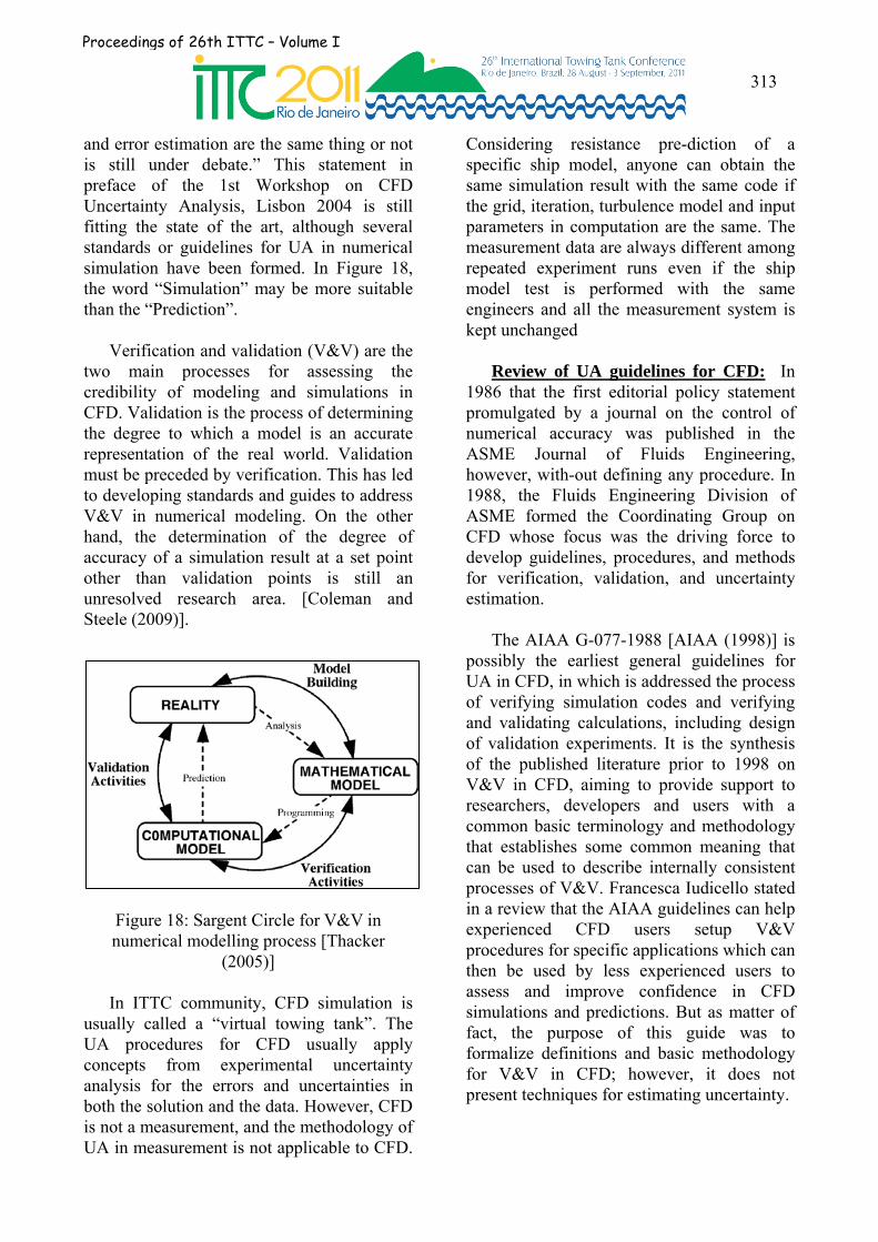
and error estimation are the same thing or not is still under debate.” This statement in preface of the 1st Workshop on CFD Uncertainty Analysis, Lisbon 2004 is still fitting the state of the art, although several standards or guidelines for UA in numerical simulation have been formed. In Figure 18, the word “Simulation” may be more suitable than the “Prediction”.

Verification and validation (V&V) are the two main processes for assessing the credibility of modeling and simulations in CFD. Validation is the process of determining the degree to which a model is an accurate representation of the real world. Validation must be preceded by verification. This has led to developing standards and guides to address V&V in numerical modeling. On the other hand, the determination of the degree of accuracy of a simulation result at a set point other than validation points is still an unresolved research area. [Coleman and Steele (2009)].

Figure 18: Sargent Circle for V&V in numerical modelling process [Thacker

(2005)]

In ITTC community, CFD simulation is usually called a “virtual towing tank”. The UA procedures for CFD usually apply concepts from experimental uncertainty analysis for the errors and uncertainties in both the solution and the data. However, CFD is not a measurement, and the methodology of UA in measurement is not applicable to CFD.

Considering resistance pre-diction of a specific ship model, anyone can obtain the same simulation result with the same code if the grid, iteration, turbulence model and input parameters in computation are the same. The measurement data are always different among repeated experiment runs even if the ship model test is performed with the same engineers and all the measurement system is kept unchanged

Review of UA guidelines for CFD: In 1986 that the first editorial policy statement promulgated by a journal on the control of numerical accuracy was published in the ASME Journal of Fluids Engineering, however, with-out defining any procedure. In 1988, the Fluids Engineering Division of ASME formed the Coordinating Group on CFD whose focus was the driving force to develop guidelines, procedures, and methods for verification, validation, and uncertainty estimation.

The AIAA G-077-1988 [AIAA (1998)] is possibly the earliest general guidelines for UA in CFD, in which is addressed the process of verifying simulation codes and verifying and validating calculations, including design of validation experiments. It is the synthesis of the published literature prior to 1998 on V&V in CFD, aiming to provide support to researchers, developers and users with a common basic terminology and methodology that establishes some common meaning that can be used to describe internally consistent processes of V&V. Francesca Iudicello stated in a review that the AIAA guidelines can help experienced CFD users setup V&V procedures for specific applications which can then be used by less experienced users to assess and improve confidence in CFD simulations and predictions. But as matter of fact, the purpose of this guide was to formalize definitions and basic methodology for V&V in CFD; however, it does not present techniques for estimating uncertainty.


314

Calculation errors are delineated by two definitions: Uncertainty: A potential deficiency in any

phase or activity of the modeling process

that is due to lack of knowledge. A recognizable deficiency in any phase or

activity of modeling and simulation that is not due to lack of knowledge.

Figure 19: Relationship between validation, calibration, and prediction (Oberkampf , 2004)


315

AIAA guide is not intended for certification or accreditation of CFD codes. AIAA focuses its procedures for bounding and controlling calculation errors. Several terms are defined as follows: Verification: The process of determining

that a model implementation accurately re-presents the developer’s conceptual description of the model and the solution to the model.

Validation: The process of determining

the degree to which a model is an accurate re-presentation of the real world from the perspective of the intended uses of the model.

Calibration: The process of adjusting

numerical or physical modeling parameters in the computational model for the purpose of improving agreement with experimental data.

Model: A representation of the physical

system or process intended to enhance our ability to understand, predict, or control its behaviour.

Modeling: The process of construction or

modification of a model. Simulation: The exercise or use of a

model. Prediction: Use of a CFD model to

foretell the state of a physical system under conditions for which the CFD model has not been validated.

The definition for verification stresses comparison with the reference standard “conceptual model”, while for validation, the standard is the “real world”. Calibration of simulation is a response to the degree of representation of the real world directed towards improvement of agreement. Calibration is commonly conducted before

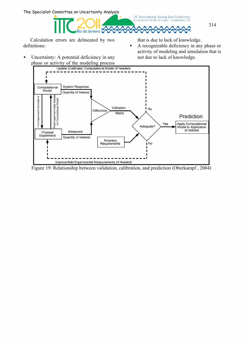
validation activities. The relationship between validation, calibration and prediction is illustrated in Figure 19. [Oberkampf (2004)]

The newly issued standard for UA in CFD is the ASME V&V 20-2009 [ASME (2009)] on November 30, 2009. A 9-members committee for this standard is formed in 2004 and chaired by Coleman. The V&V 20 was introduced to the 3rd Workshop on CFD Uncertainty Analysis, Lisbon 2008 and adopted as validation procedure. According to Coleman and Steele (2009) and Coleman (2008), the V&V 20 approach was initially proposed by Coleman and Stern (1997) and originated from ONR Program 1996-2000 in which two RANS codes are used and experiments on models are carried out in three towing tanks in USA (DTMB, IIHR) and Italy (INSEAN).

No methodology is available for prediction uncertainty analysis. Consideration of the accuracy of simulation at points other than the validation points is a matter of engineering judgment specific to each family of problems.

The ASME Standard uses the definitions of verification and validation used that are consistent with those in AIAA guideline.

Verification is now commonly divided into two types: code verification and solution verification as defined as Code/Software verification: The process

of determining that the numerical algorithms are correctly implemented in the computer code and of identifying errors in the software.

Solution/Calculation verification: The

process of determining the solution accuracy of a particular calculation.

Before uncertainty estimation, the code itself must be first verified. Code verification


316

is to determine the code is free of mistakes and directed towards [Oberkampf (2004)]: Finding and removing mistakes in the

source code; Finding and removing errors in numerical

algorithms; Improving software using software

quality assurance practices.

Solution verification is the process to estimate the numerical uncertainty required for the validation process. Solution verification activities are directed toward [Oberkampf (2004)]: Assuring the accuracy of input data for

the problem of interest; Estimating the numerical solution error; Assuring the accuracy of output data for

the problem of interest.

The recommended approach for code verification of RANS solvers is the use of the Method of Manufactured Solution (MMS) [Eça et al. (2005)]. The MMS assumes a sufficiently complex solution form so that all the terms in the Partial Differential Equations (PDEs) are exercised. This particular technique is usually more of a developer's tool, and code verification is commonly assumed to be completed; especially for those extensively used commercial codes, although code verification is not the exclusive responsibility of code developers.

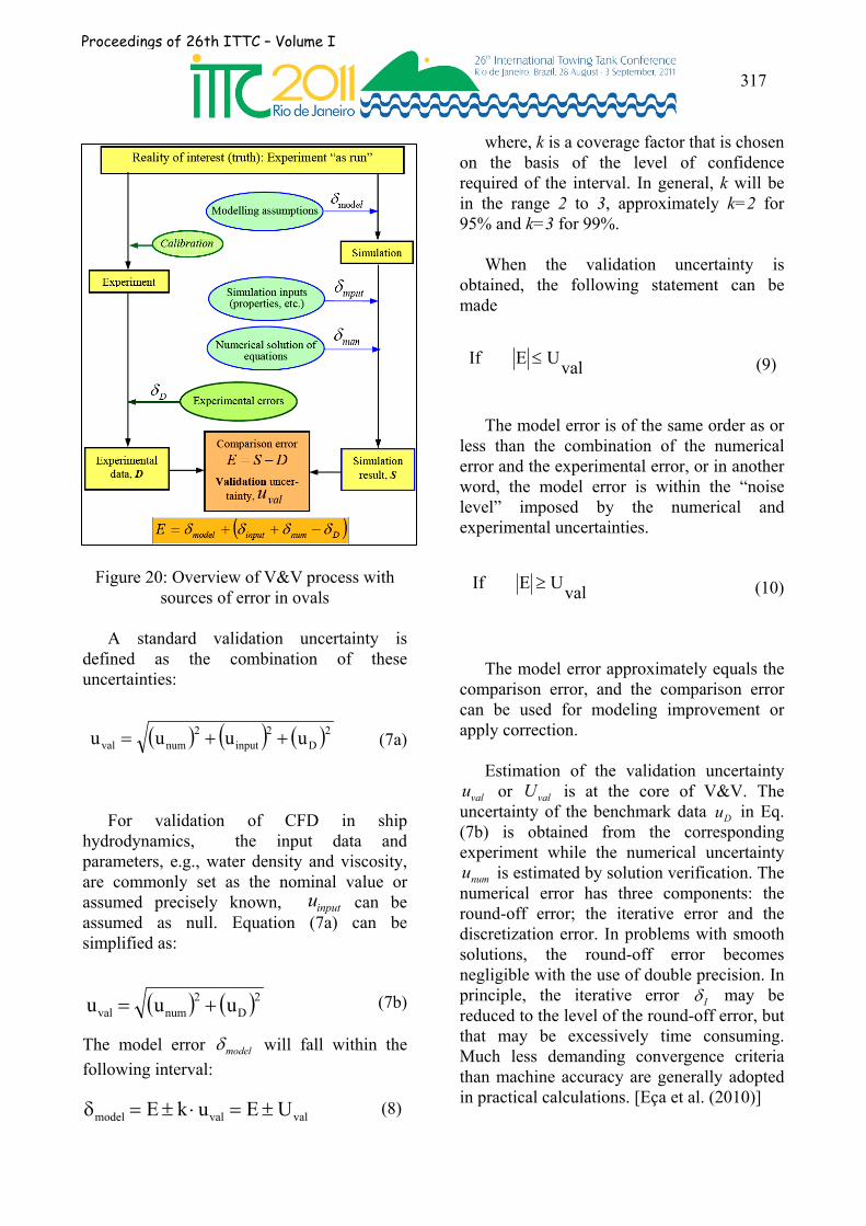
The validation in ASME V&V 20 is shown schematically in Figure 20. The validation comparison error E is defined as [Coleman and Steele (2009)]

(4)

where, S is the simulation solution, D the experimental data, T the true value (unknown) of the reality of interest, S the error in the

simulation solution and D the error in the experiment data.’

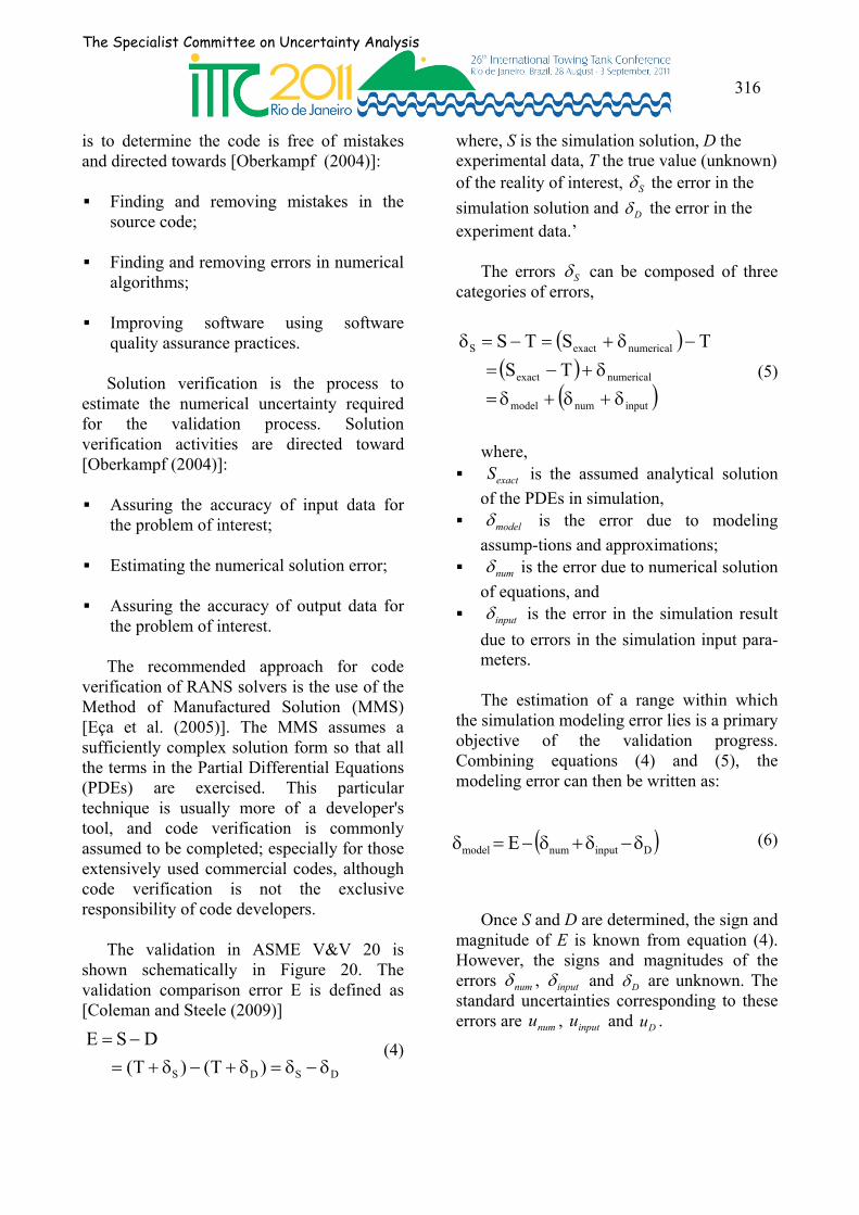
The errors S can be composed of three categories of errors,

(5)

where, exactS is the assumed analytical solution

of the PDEs in simulation, model is the error due to modeling

assump-tions and approximations; num is the error due to numerical solution

of equations, and input is the error in the simulation result

due to errors in the simulation input para-meters.

The estimation of a range within which the simulation modeling error lies is a primary objective of the validation progress. Combining equations (4) and (5), the modeling error can then be written as:

(6)

Once S and D are determined, the sign and magnitude of E is known from equation (4). However, the signs and magnitudes of the errors num , input and D are unknown. The standard uncertainties corresponding to these errors are numu , inputu and Du .

inputnummodel

numericalexact

numericalexactS

TS

TSTS

Dinputnummodel E

DSDS )T()T(

DSE


317

Figure 20: Overview of V&V process with

sources of error in ovals

A standard validation uncertainty is defined as the combination of these uncertainties:

(7a)

For validation of CFD in ship hydrodynamics, the input data and parameters, e.g., water density and viscosity, are commonly set as the nominal value or assumed precisely known, inputu can be assumed as null. Equation (7a) can be simplified as:

(7b)

The model error model will fall within the

following interval:

(8)

where, k is a coverage factor that is chosen on the basis of the level of confidence required of the interval. In general, k will be in the range 2 to 3, approximately k=2 for 95% and k=3 for 99%.

When the validation uncertainty is obtained, the following statement can be made

(9)

The model error is of the same order as or less than the combination of the numerical error and the experimental error, or in another word, the model error is within the “noise level” imposed by the numerical and experimental uncertainties.

(10)

The model error approximately equals the comparison error, and the comparison error can be used for modeling improvement or apply correction.

Estimation of the validation uncertainty

valu or valU is at the core of V&V. The uncertainty of the benchmark data Du in Eq. (7b) is obtained from the corresponding experiment while the numerical uncertainty

numu is estimated by solution verification. The numerical error has three components: the round-off error; the iterative error and the discretization error. In problems with smooth solutions, the round-off error becomes negligible with the use of double precision. In principle, the iterative error I may be reduced to the level of the round-off error, but that may be excessively time consuming. Much less demanding convergence criteria than machine accuracy are generally adopted in practical calculations. [Eça et al. (2010)]

2D2

input2

numval uuuu

2D2

numval uuu

valvalmodel UEukE

valU E If

valU E If


318

Grid refinements studies in solution verification provide an estimate of the discretization error G and, the most-widely-used estimation method is classical Richardson extrapolation (RE), G ≈ RE . Uncertainty esti-mates at a level of confidence 95% can then be calculated by Roache’s grid convergence index (GCI) that is obtained by multiplying the (generalized) RE error estimate, RE , by an empirically determined factor of safety, FS, as:

(11)

(12)

where iS is the simulation solution by the ith grid, 0S is the estimated exact solution (unknown), ih is a parameter representing the grid cell size, α and p are unknown constants. Therefore, at least three grids are required to determine the three unknowns ( 0S , α and p).

Generally, these grids must be geometrically similar and in the asymptotic range. Meanwhile, the iterative error should be reduced to negligible levels, i.e., being 2 to 3 orders of magnitude smaller than the discretization error.

For a gird triplet, a uniform refinement ratio between solutions is:

(13)

where the grid size parameter is:

(14)

The convergence ratio is defined as:

(15)

When 0<R<1 (monotonic convergence), the numerical error of the fine gird is estimated by (generalized) RE according to Eq. (12).

(16)

(17)

When more than 3 grids are used to estimate GCI, the least-squares method pioneered by Eça and Hoekstra is cited [ASME (2009)] as the most robust and tested method available for the prediction of numerical uncertainty as of this date. Three unknowns, 0S , α and p, are simultaneously computed by a least squares root approach that minimizes the function.

(18)

if 3Gn . Then, the RE error is obtained:

(19)

The fitting standard deviation Gsu is

(20)

1h

h

h

hr

2

3

1

2G

pG

2101RE r1

SS

G21

32

21

32pG rln/lnp;r

Gn

i

2pi0i0 )hS(S)p,,S(

01RE SS

3n

)hS(Su

G

n

i

2pi0i

Gs

G

RESG FUGCI

pi0iRE hSSS

31

ii )N( Cells ofNumber

Domainncalculatio of Volumeh

32

21

23

12

SS

SSR


319

regarded as one of the contributions of numerical uncertainty and included in the grid uncertainty GU in the way that is modified in this report.

(21)

where, the factor of safety, FS, is chosen according to the so-called observed order of accuracy (rate of convergence), p, as [Eça et al. (2003)].

(22)

In the case of oscillatory convergence, i.e., R<0 in Eq. (15), the grid uncertainty may be estimated by bounding the error based on the oscillation maximums US and minimums LS

(23a)

(23b)

The resulting uncertainty from equation (23a) is some kind of limit that may be approximately regarded as at a level of confidence 99%. The corresponding uncertain-ty at a level of confidence 95% is recommend-ed in this report to be approximated as

(24)

ITTC Practices. ITTC recommended its interim procedures (4.9-04-01-01 and 4.9-04-01-02) for UA in CFD simulation as early as in the 23rd ITTC). The latest reversion of UA procedure for CFD is recommended by the 25th ITTC [ITTC (2008a)]. Fred Stern [e.g., Stern et al. (1999) and (2006), ITTC (2008c) and Larsson et al. (2010)] has been making one of the most significant contributions to ITTC in this field.

The ITTC procedure is very detailed for estimating the uncertainty in a simulation result. It is intended for practical use and presented in an easily implemented way. The latest workshop on CFD – Gothenburg 2010 was held on 8-10 December 2010. It was the sixth of series of workshops since 1980 [Larsson et al. (2010)]. Over 30 organizations have taken part in the activities of Gothenburg 2010.

Most of those organizations which had performed V&V and presented uncertainty results complied with the ITTC (2008a) approach for uncertainty estimation of CFD simulation. Several exceptions exist as follows: VTT used 9 grids to estimate the

numerical uncertainty by the least-squares method proposed by Eça and Hoekstra [ASME (2009)].

SSPA: the proposed method of Eça and

2%)95(Gs

2

2Gs%95

2

RES%95G

UCGI

utFU

5.0p,5.4p5.3 if 3F

5.4p,5.3p5.0 if25.1F

S

S

LU SS2

1GCI

LU

LU%)95(

SS3

1

SS2

1

3

12GCI

2%95D2

%95G

2D%95

2

%95G%95val

UU

ukUU


320

Hoekstra. Southampton/QinetiQ: the ASME V&V

20

Figure 21: Example of grid refinement study for the turbulent flow over a flat plate [Eça (2010)]

One of distinguishable aspects in the ITTC (2008a) procedure is the introduction of the ‘correction factor’ verification method that was proposed by Stern et al. (2001), although there is still some argument on it [Wilson et al. (2004)]. The correction factor is just one of alternatives of the safety factor method [Roache, (1997)] which is determined by a much less complex approach than that of the former. However, the least-squares method proposed by Eça and Hoekstra, which is based on the Richardson extrapolation, is not included in the ITTC (2008a).

Another novel concept introduced in the ITTC (2008a) procedure other than AIAA and ASME guides is that the numerical error num is divided into two components:

(25)

where, *num is an estimate of magnitude and

deterministic sign of num and num is the error

in the estimate. On another word in this report, num falls within the following

interval:

(26)

where, *numu

is the standard uncertainty of num .

Then the corrected simulation is defined as

(27)

If the input and iterative errors are omitted, the corrected simulation error is represented as

(28)

Then, the corrected validation uncertainty is:

(29a)

(29b)

The model error can be rewritten as:

(30)

However, considering Eq. (15) can be rewritten as:

(31)

num*numnum

*numC SS

2D

2*num

Cval uuu

2D%95

2*numS

Cval ukuFU

Cval

*num

CvalCmodel UEUE

32

21

2C3C

1C2C

*num2

*num3

*num1

*num2

23

12

SS

SS

SS

SS

SS

SSR

nummodelSC

num%95*numnum uk


321

Introduction of the novel error *num will

lead to the same estimate of the numerical uncertainty as that of Eq. (16) when Richardson extrapolation is used. But the model error estimate resulted from Eq. (30) may be different from that of Eq. (8).

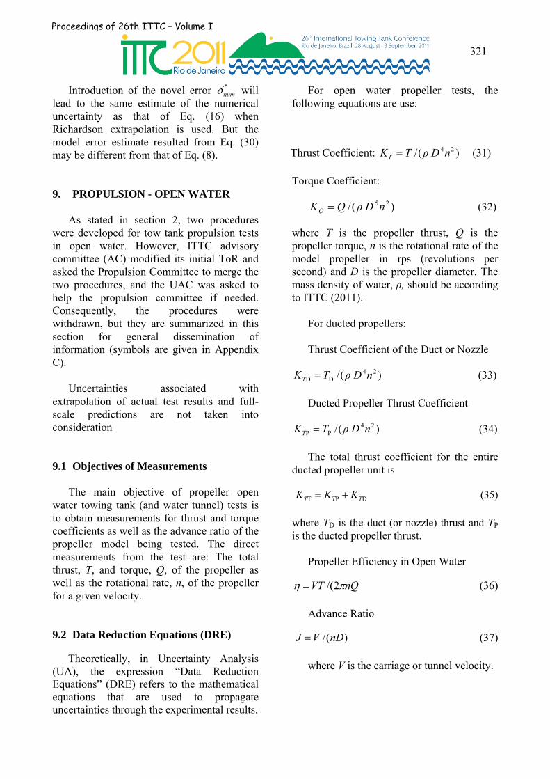
9. PROPULSION - OPEN WATER

As stated in section 2, two procedures were developed for tow tank propulsion tests in open water. However, ITTC advisory committee (AC) modified its initial ToR and asked the Propulsion Committee to merge the two procedures, and the UAC was asked to help the propulsion committee if needed. Consequently, the procedures were withdrawn, but they are summarized in this section for general dissemination of information (symbols are given in Appendix C).

Uncertainties associated with extrapolation of actual test results and full-scale predictions are not taken into consideration

9.1 Objectives of Measurements

The main objective of propeller open water towing tank (and water tunnel) tests is to obtain measurements for thrust and torque coefficients as well as the advance ratio of the propeller model being tested. The direct measurements from the test are: The total thrust, T, and torque, Q, of the propeller as well as the rotational rate, n, of the propeller for a given velocity.

9.2 Data Reduction Equations (DRE)

Theoretically, in Uncertainty Analysis (UA), the expression “Data Reduction Equations” (DRE) refers to the mathematical equations that are used to propagate uncertainties through the experimental results.

For open water propeller tests, the following equations are use:

Thrust Coefficient: )(/ 24nρ DTKT (31)

Torque Coefficient:

nρ DQKQ )(/ 25 (32)

where T is the propeller thrust, Q is the propeller torque, n is the rotational rate of the model propeller in rps (revolutions per second) and D is the propeller diameter. The mass density of water, ρ, should be according to ITTC (2011).

For ducted propellers:

Thrust Coefficient of the Duct or Nozzle

)(/ 24DD nρ DTKT (33)

Ducted Propeller Thrust Coefficient

)(/ 24PP nρ DTKT (34)

The total thrust coefficient for the entire ducted propeller unit is

DPT TTT KKK (35)

where TD is the duct (or nozzle) thrust and TP is the ducted propeller thrust.

Propeller Efficiency in Open Water

nQVT 2/( (36)

Advance Ratio

)(/ nDVJ (37)

where V is the carriage or tunnel velocity.


322

9.3 Description of Uncertainty Sources

From uncertainty analysis, the entire testing process of an open water propeller in a towing tank or water tunnel test may be grouped into five blocks as shown in Figure

22 Each block is reserved for one group of uncertainty sources.

Figure 22: Schematic diagram of whole test system

a) Geometry.

No. ① block lists the uncertainty sources related to propeller model geometry, including the errors from manufacturing and deformation during test. The model propeller is manufactured per the geometric specifications of the real propeller, but uncertainties in dimensions, offsets, and tolerances can occur in diameter, chord length, pitch, and blade section shape. The influence of these errors in dimensions and shape can affect the flow characteristics

around the propeller blades and hence the measured thrust and torque.

With the existence of laser based measurement systems and modern machining methods, the deviations of the manufactured propeller can be measured relative to the design with high precision. However, the effect of any deviations on propeller performance is difficult to quantify; consequently, only the uncertainty in the diameter is considered.


323

b) Installation.

No.② block outlines the uncertainty sources related to the propeller model installation/alignment. The drive shaft should be arranged parallel to the calm water surface and the carriage rails. The propeller immersion has to be selected such that air drawing from the water surface is avoided at any test condition. ITTC 7.5-0.2-03-02.1 (2008a) recommends an immersion of at least 1.5 diameters.

If a current meter is used to measure the speed of advance of the propeller model the immersion of it should correspond to the immersion of the propeller shaft. The distance between the propeller and the current meter should be chosen to ensure that the current meter does not influence the propeller during the test.

c) Calibration.

No.③ block shows the uncertainty sources related to the calibration of the measurement instruments. Guidelines for uncertainties in instrument calibration are described in ITTC (2008b). Manufacturer uncertainties in instruments can be obtained directly from the design specification sheets. All calibration results should be traceable to a National Metrology Institute (NMI).

d) Direct Measurement.

No.④ block indicates the uncertainty sources related to the time history of sampling data or human readings. For the data acquisition system (DAS), the sampling rate, the length of data sample, and the frequency of low-pass filter may affect the values of measurement. The effect of the data acquisition system on uncertainty of measurement is preferably included in the calibration by a through system or end-to-end

calibration. That is, the instruments are calibrated on the data acquisition system for the test.

e) Data Reduction.

No.⑤ block outlines the uncertainty sources related to the data reduction process and all the plotted curves. The dimensions of the tank should be large enough to avoid blockage. For a towing tank test, ITTC (2008c) outlines three methods for blockage corrections for towing tank tests.

9.4 Uncertainty in Thrust & Torque a) Propeller Geometry

As indicated previously, an easy verification of accuracy in geometry is to perform multiple tests with different propeller models manufactured to the same surface design specifications or drawings. For the uncertainty estimates, only the uncertainty in the propeller diameter is considered. ITTC (2002a) specifies a manufacturing tolerance of ±0.10 mm for the model diameter; however, the directly measured diameter and its uncertainty should be applied in the analysis. b) Propeller model installation

The installation of the propeller model should be done according to Section 3.1.2 of ITTC (2008a). c) Instrument Calibration

Calibration should be performed by the end-to-end method so that details of uncertainty analysis of signal conditioning and data acquisition systems are not necessary. Such a calibration exercise should be regarded as independent of the open water test, so that the uncertainty analysis of


324

calibration will be separately estimated and reported. The elements of the calibration process are outlined in the following paragraphs. Additional details and the original sources are described in ITTC (2008b). d) Force Calibration

Force calibrations, including body forces, moments, and propeller thrust and torque, are usually calibrated with masses on a calibration stand. In that case, force, F, is related to mass, m, by the following:

)1( wa /mgF (38a)

or for a calibration stand with force multiplying levers

)/1)(/( wa12 LLmgF (38b)

where m is the mass, g is local acceleration of gravity, a is air density, w is the density of the weight, and L1 and L2 are the lengths of the levers. For a calibration stand, torque is then

FLQ (39)

where L is the length of the moment arm.

The last term of Equations (38a) and (38b) is a buoyancy correction. Local gravity can differ from standard gravity, 9.80665 m/s2, on the order of 0.1 %, and the buoyancy correction is typically 0.017 %. Mass sets commonly applied to force calibrations have a specification on the order of 0.01 %. Consequently, the correction for local gravity can be 10 times the uncertainty in the reference mass.

During calibration, the force is changed by adding or removing weights. The mass in Equation (38) is then given by

n

iimm

1

(40)

The weight set is usually calibrated as a set at the same time against the same reference standard. In that case, the uncertainty in the weights is assumed to be perfectly correlated. The standard uncertainty in the total mass is then

n

iim uu

1

(41)

where ui is the standard uncertainty of the i-th weight mi.

With the assumption that the contributions in the uncertainty in the air and weight densities are small compared to the other terms, the combined relative uncertainty in the applied force or thrust from Equation (38b) is

222

211

22

r

)/()/()/()/(

/)(

LuLugumu

FFu

LLgm

(42)

If the calibration stand does not include a force multiplier levers, the uncertainty in the lever arm lengths will be zero in Equation (32). From Equations (38a) and (39), the relative uncertainty in torque is

(43)

The thrust and torque balances should be calibrated with the same data acquisition system used in the test. Nominally, the calibration curve should be linear. Linear regression analysis will then produce the slope and intercept for the conversion of digital volts to force units during the test.

The combined uncertainty in calibration consists of three elements: (1) ur, uncertainty in the reference standard from Equations (42) and (13), (2) uA, Type A uncertainty from the standard deviation during data collection with

222r )/()/()/(/)( LugumuQQu Lgm


325

the DAS for each data point, and (3) ucf, uncertainty in the curve fit from calibration theory in ITTC (2008b). The combined standard uncertainty in calibration from these three elements is estimated from the following for thrust

)()()()( 2cf

2r

2A FuFuFuFu (44)

and for torque

)()()()( 2cf

2r

2A QuQuQuQu (45)

Equations (44) and (45) are, then, a Type B when they are applied in a test.

9.5 Direct Measurements a) Thrust

Although the open water test is steady, the thrust signal recorded by data acquisition system (DAS) will vary with time due to instabilities of the flow, test-rig vibration, electro-magnetic interference, drift of measuring system, fluctuation of power supply, electronic noise, and other unknown interference. The measurement of the thrust by DAS at each speed is obtained by averaging the time history of the thrust signal in a interval of time, T =n/fs

n

iiTnT

1

)/1( (46)

where T is the average thrust, fs is the sampling rate, n the number of the samples, Ti the i-th data of the sample. The uncertainty in Equation (46) is computed by the Type A uncertainty method described in the general guideline on uncertainty ITTC (2008b). The uncertainty is then the standard deviation of the mean of T given by

nsuu TT /A (47)

where sT is the standard deviation computed from Ti.

The combined standard uncertainty of the thrust can be estimated from the Type A and Type B uncertainties by

22BAT uuu (48)

where uA is from Equation (47) and uB from Equation (44).

In some cases, repeat measurements on the order of 10 may be necessary for establishment of a better uncertainty estimate. An example of the importance of repeat measurements is described by Forgach (2002). b) Torque

The procedure for uncertainty estimates in thrust can be applied also to the torque. The uncertainty in the reference torque at calibration is given by Equation (43), and the combined uncertainty during calibration is given by Equation (35). The Type A uncertainty for torque during the test is

nsuu QQ /A (49)

2B

2A uuuQ (50)

where uA is from Equation (39) and uB from Equation (35). c) Rotational Rate

In naval hydrodynamic applications, rotational rate is a commonly measured parameter as shaft rotational rate in propeller performance. Rotational rate is measured from a pulse-generating device such as an optical encoder or steel gear with a magnetic pick-up. These devices are inherently digital. Data acquisition cards typically include a 16-bit analogue to digital converter, counter


326

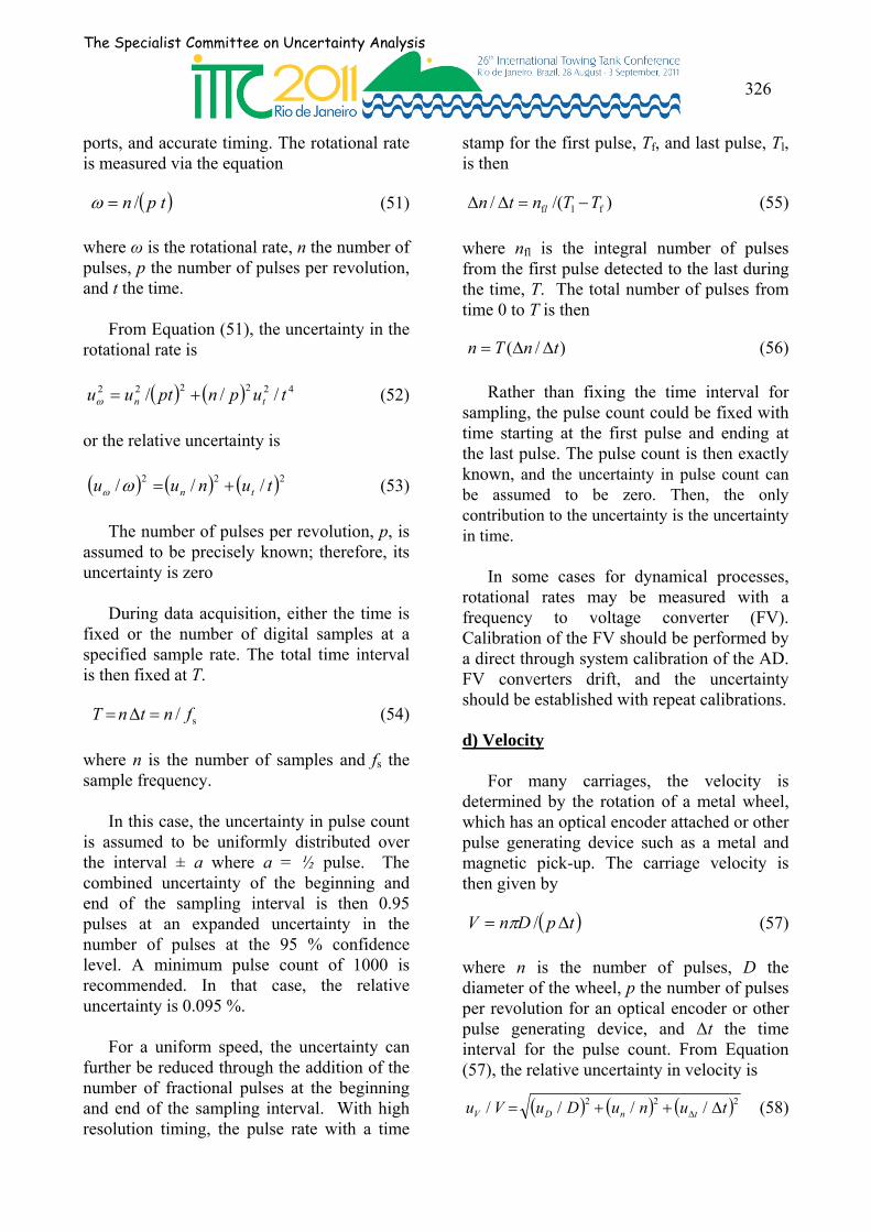
ports, and accurate timing. The rotational rate is measured via the equation

tpn / (51)

where ω is the rotational rate, n the number of pulses, p the number of pulses per revolution, and t the time.

From Equation (51), the uncertainty in the rotational rate is

422222 /// tupnptuu tn (52)

or the relative uncertainty is

222 /// tunuu tn (53)

The number of pulses per revolution, p, is assumed to be precisely known; therefore, its uncertainty is zero

During data acquisition, either the time is fixed or the number of digital samples at a specified sample rate. The total time interval is then fixed at T.

s/ fntnT (54)

where n is the number of samples and fs the sample frequency.

In this case, the uncertainty in pulse count is assumed to be uniformly distributed over the interval ± a where a = ½ pulse. The combined uncertainty of the beginning and end of the sampling interval is then 0.95 pulses at an expanded uncertainty in the number of pulses at the 95 % confidence level. A minimum pulse count of 1000 is recommended. In that case, the relative uncertainty is 0.095 %.

For a uniform speed, the uncertainty can further be reduced through the addition of the number of fractional pulses at the beginning and end of the sampling interval. With high resolution timing, the pulse rate with a time

stamp for the first pulse, Tf, and last pulse, Tl, is then

)/(/ flf TTntn l (55)

where nfl is the integral number of pulses from the first pulse detected to the last during the time, T. The total number of pulses from time 0 to T is then

)/( tnTn (56)

Rather than fixing the time interval for sampling, the pulse count could be fixed with time starting at the first pulse and ending at the last pulse. The pulse count is then exactly known, and the uncertainty in pulse count can be assumed to be zero. Then, the only contribution to the uncertainty is the uncertainty in time.

In some cases for dynamical processes, rotational rates may be measured with a frequency to voltage converter (FV). Calibration of the FV should be performed by a direct through system calibration of the AD. FV converters drift, and the uncertainty should be established with repeat calibrations. d) Velocity

For many carriages, the velocity is determined by the rotation of a metal wheel, which has an optical encoder attached or other pulse generating device such as a metal and magnetic pick-up. The carriage velocity is then given by

tpDnV / (57)

where n is the number of pulses, D the diameter of the wheel, p the number of pulses per revolution for an optical encoder or other pulse generating device, and Δt the time interval for the pulse count. From Equation (57), the relative uncertainty in velocity is

(58) 222 //// tunuDuVu tnDV


327

The diameter D can be measured very accurately with a laser scanning coordinate system. Normally, a computer data acquisition card (DAC) normally has a counter port and very accurate timing. Repeat measurements of the carriage speed, at least 10 at a single speed, may be necessary for more accurate estimate in carriage speed uncertainty as described by Forgach (2002).

9.6 Uncertainty in Propeller Coefficients

The results of uncertainty analysis for propeller performance have been described previously as an example in ITTC (2008d). The results are repeated in the following sections. a) Thrust Coefficient

From Equation (31), the combined relative uncertainty for the thrust coefficient is

2

D2

n

2t

2T

2TK

)D/u4()n/u2(

/t/u)T/u()K/u(T

(59)

where the uncertainty in water density equation is assumed small in comparison to the contribution from water temperature, t. In general, the water temperature, rotational rate, and total thrust may be acquired with a data acquisition system (DAS); consequently, the uncertainty estimate will include estimates from both Type A and Type B methodologies. b) Torque Coefficient

From Equation (32), the combined relative uncertainty for the torque coefficient is

(60)

c) Advance ratio

The combined relative uncertainty for the advance coefficient, from Equation (37), is

222 //// DunuVuJu DnVJ (61)

d) Propeller Efficiency

From Equation (36), the combined relative uncertainty for the propeller efficiency is

2

2222

)/(

)/()/()/()/(

nu

QuTuVuu

n

QTV

(62)

10. REPORTING UNCERTAINTIES

Report of uncertainty analysis in the open water test document can be given as a table in which the following information and data are summarized: All the dominant uncertainty sources and

components related to the measurements (thrust, torque, rotational rate, velocity, coefficients, etc.);

The type of evaluation method for each

uncertainty component; The expressions of sensitivity

coefficients for each component to the desired measurands (thrust, torque, advance coefficient and propeller efficiency);

The combined standard uncertainty of

the desired measurands; The expanded uncertainty at the 95 %

confidence limit, usually with the coverage factor k = 2, for the desired measurands;

The information on propeller model

geometry verification, mainly the

22

222

)/5()/2(

//)/()/(

Dunu

tuQuKu

Dn

tQQKQ


328

uncertainty of model diameter; Documentation of calibration results with

their uncertainties and statement of traceability to an NMI.

Additionally, data should be presented graphically whenever possible. Calibration data should be plotted as residual plots as described in ITTC (2008b).

11. UA – SIMPLE BEST PRACTICE Uncertainty depends on the entire towing

tank testing process, and any changes in the process can affect the uncertainty of the test results.

Uncertainty assessment methodology

should be applied in all phases of the towing tank testing process including design, planning, calibration, execution, and post-test analyses. Uncertainty analysis should be included in the data processing codes.

Simplified analysis by prior knowledge,

such as a database, tempered with engineering judgment is suggested. Dominant error sources should be identified, and effort focused on those sources for possible reduction in uncertainty.

Through system or end-to-end

calibrations should be performed with the same DAS and software for the test. A database of the calibrations should be maintained so that new calibrations can be compared to previous ones.

A laboratory should have a benchmark

test with uncertainty estimates that is repeated periodically. A benchmark test will insure that the equipment, procedures, and uncertainty estimates are adequate.

A reference test condition in a test series should be repeated about 10 times in sequence as a better measure of uncertainty and check on uncertainty estimates. Also, reproducibility of test results for a representative test condition should be checked in a long duration test of more than one day with a test at the beginning, middle, and end of the test series.

Together with uncertainty report, the

following statements should be included in the test documentation: a. Towing tank or water tunnel test

process, measurement systems, and data streams in block diagrams.

b. Equipment and procedures used.

The ITTC “Example for Open water Test” ITTC Procedure 7.5-02-03-02.2 (2002b) also contains data that may be updated for consistency with the present procedure. The uncertainty analysis based on the above data will give a practical guide for identification of the dominant uncertainty components.

12. THE 1978 QUESTION

In Section 2, the 26 ITTC ToR document requested the development of a procedure for “Uncertainty Analysis for the 1978 ITTC 3P Method, liaise with the Propulsion Committee. This task was not performed, but will discussed during the 26th ITTC (2011) general meeting (UAC presentation).

The same task was also mandated by the 25th ITTC, and the task was not performed. It was postponed to the 26th ITTC.

To the UAC, the objective for this procedure was not clear, and its wording was vague. After discussions with the 25th AC and the 3P committee, it was understood that the objective of the AC is to use the procedure to determine which propulsion method is superior: the 1978 method or the more recent


329

method suggested by the propulsion committee.

Fundamentally, UA cannot be used to determine which experiment is better. The purpose of UA is to establish the quality of the data. ISO-GUM guidelines deal with uncertainty estimates in measurements (in numbers) for the 95% confidence level. The UA will not help users to decide which experiment is superior. That decision should be based on the physics and mechanics of the problem. This statement was also made during the 25th ITTC (2008) (UAC presentation).

For this particular task, a discussion will be prepared and it will be presented for the 2011 ITTC general conference in Brazil.

13. REFERENCES

AIAA/GTTC IBT WG, 2003, Recommended Practice, Calibration and Use of Internal Strain-Gauge Balances with Application to Wind Tunnel Testing, AIAA R-091-2003

ASME, 2009, “Standard for Verification and Validation in Computational Fluid Dy-namics and Heat Transfer,” V&V 20 - 2009, American Society of Mechanical Engineers, New York.

ASTM E28.01, 2006, ASTM E74-06: Standard Practice of Calibration of Force-Measuring Instruments for Verifying the Force Indication of Testing Machines.

Bergmann, R., Philipsen, I., 2010, Some Contemplations on a Proposed Definition of Uncertainty for Balances, 7th International Symposium on Strain-Gauge Balances, 10-13 May 2010, Williamsburg, VA

USABergmann, R., Philipsen, I., 2010, An experimental comparison of different load tables for balance calibration, 7th

International Symposium on Strain-Gauge Balances, 10-13 May 2010, Williamsburg, VA USA

Cahill, D. M., 2008, Balance Calibration Uncertainty Introduction to Discussion on Standardization, 6th International Symposium on Strain-Gauge Balances, 5-8 May 2008, Zwolle, The Netherlands

EAL Committee 2, 1996, EAL-G22: Uncertainty of Calibration Results in Force Measurements

Forgach, K. M., 2002, “Measurement Uncertainty Analysis

Hufnagel, K., 2010, Common Definition of Balance Accuracy and Uncertainty, 7th International Symposium on Strain-Gauge Balances, 10-13 May 2010, Williamsburg, VA USA

Harvey, A. H., Peskin, A. P., and Klein, S. A., 2008, “NIST/ASME Steam Properties Version 2.22: Users’ Guide,” National Institute for Standards and Technology, Gaithersburg, Maryland, USA.

IAPWS, 2008a, “Supplementary Release on Properties of Liquid Water at 0.1 MPa,” The International Association for the Properties of Water and Steam, Berlin.

IAPWS, 2008b, “Release on the IAPWS Formulation 2008 for the Thermodynamic Properties of Seawater” The International Association for the Properties of Water and Steam, Berlin.

IOC, SCOR, and IAPSO, 2010, “The interna-tional thermodynamic equations of seawater – 2010: Calculation and use of thermodynamic properties,” Intergovernmental Oceanographic Commission, Manuals and Guides No. 56, UNESCO, 196 pp.

ISO TC 164/SC 1, 2004, ISO 376: 2004,


330

Metallic materials -- Calibration of force-proving instruments used for the verification of uniaxial testing machines

ITTC, 2008a, “Guide in the Expression of Uncertainty in Experimental Hydrodynamics,” ITTC Procedure 7.5-02-01-01, Revision 01.

ITTC, 2008b, “Uncertainty Analysis - Instrument Calibration,” ITTC Procedure 7.5-01-03-01.

ITTC, 2008c, “Testing and Data Analysis Methods, Resistance Test,” ITTC Procedure 7.5-02-02-01.

ITTC, 2008d, “Guidelines for Uncertainty Analysis in Resistance Towing Tank Tests,” ITTC Procedure 7.5-02-02-02.

ITTC, 2011, “Fresh Water and Seawater Properties”, ITTC Procedure 7.5-02-01-03, Revision 01.

JCGM, 2008a, “Evaluation of measaurement data – Guide to the expression of uncertainty in measurement,” JCGM 100:2008 GUM 1995 with minor corrections, Joint Committee for Guides in Metrology, Bureau International des Poids Mesures (BIPM), Sèvres, France.

JCGM, 2008b, “International vocabulary of metrology – Basic and general concepts and associated terms (VIM),” JCGM 200:2008, 3rd Edition, Joint Committee for Guides in Metrology, Bureau International des Poids Mesures (BIPM), Sèvres, France.

JCGM, 2008c, “Evaluation of measurement data – Supplement 1 to the “Guide to the expression of uncertainty in measurement” – Propagation of distributions using a Monte Carlo method,” JCGM 101:2008, Joint Committee for Guides in Metrology, Bureau International des Poids Mesures (BIPM), Sèvres, France.

JCGM, 2009, “Evaluation of measurement data – An introduction to the ‘Guide to the expression of uncertain in measurement” and related documents,’ JCGM 104:2009, Joint Committee for Guides in Metrology, Bureau International des Poids Mesures (BIPM), Sèvres, France.

Lin, Alan C. M., 1982, “Bare Hull Effective Power Predictions and Bilge Keel Orientation for DDG 51 Hull Represented by Model 5415,” Technical Report DTNSRDC/SPD-200-03, David W. Taylor Naval Ship Research and Development Center, Bethesda, Maryland, USA.

Longo, J. and Stern, F., 1998, “Resistance, Sinkage and Trim, Wave Profile, and Nominal Wake and Uncertainty Assessment for DTMB Model 5512,” Proceedings of the 25th American Towing Tank Conference, Iowa City, IA.

Park, J. T., Ratcliffe, T. J., Minnick, L. M., and Russell, L. E., 2010a, “Test Results and Uncertainty Estimates for CEHIPAR Model 2716,” Proceedings of the 29th American Towing Tank Conference, Annapolis, Maryland, USA, pp. 219-228.

Park, J. T., Ratcliffe, T. J., Minnick, L. M., and Russell, L. E., 2010b, “Uncertainty Analysis of Resistance and Sinkage and Trim Measurements Obtained on CEHIPAR Model 2716, Report NSWCCD-50-TR—2010/041, Maryland, USA.

Sharqawy, Mostafa H., Lienhard V, John H., and Zubair, Syed M., 2010, “Thermophysical properties of seawater: a review of existing correlations and data,” Desalination and Water Treatment, Vol. 16, pp. 354-380.

Thompson, A. and Taylor, B. N., 2008, “Guide for the Use of the International System of Units (SI),” NIST Special Publication 811, National Institute of


331

Standards and Technology, Gaithersburg, Maryland.

Ulbrich, N., Volden, T., 2010, Regression Model Term Selection for the Analysis of Strain-Gage Balance Calibration Data, 7th International Symposium on Strain-Gauge Balances, 10-13 May 2010, Williamsburg, VA USA

14. APPENDIX A: CONFIDENCE THROUGH UNCERTAINTY

All tow tanks and ocean technology research groups are working on a mega Science and Technology (S&T) project called Experimental Uncertainty Analysis (EUA). By and large, Uncertainty Analysis (UA) has two main sections: a) Section # 1 is “Objective Uncertainty Analysis, OUA, and 2) Section # 2 is “Subjective Uncertainty Analysis, SUA. By far, the OUA is what we do best in tow tanks. If a new technology is needed (such as development of an environmentally safe offshore platform in the Arctic for oil and gas exploitation), and we are not sure how to design it, due to the lack of factual data and scientific knowledge; we call it research and development (R&D). Then, we spend money and efforts to acquire data and gain the knowledge necessary to understand (and build) that Arctic platform. In many ways, the purpose of tow tanks is to shed light on the unknown, reduce uncertainties, and eliminate risks surrounding the achievement of our human goals.

Also, in tow tanks, we face SUA. Using our collective experience, S&T sixth sense developed over many years of practice, and the scientific traditional burning desire to figure out and develop new things and products will help to reduce the “feeling” of uncertainties substantially. Armed with actual knowledge and a good assessment of uncertainties and potential risks, scientists will decide on the best possible way on how

to build that Arctic platform (or not to build it at all).

The science of measurement is rooted in our human desire to learn and figure out new things, and to control our life on earth and its environment. About 3000 years ago, the Pharaoh of ancient Egypt, invented a unit length called the royal cubit (a distance from the elbow to the tip of the middle finger), and if a pyramid was built without the use of a highly calibrated cubit, the Pharaoh’s police will certainly punish the Project Manager (PM) and probably everyone else on his/her team.

The Greeks ignored the idea of using their arms to measure lengths. Instead, they used their feet. Consequently the “foot” as a unit length emerged. From the foot, other units such as the step, the yard, and the mile have been developed. Like ancient Egyptians, the Greeks also demanded accuracy in measurements and enforced strict rules for instrument calibration.

Centuries later, someone in the 16th century (Simon Stevin) started talking about using a decimal fraction in measurements “he called it the tenth”. Almost 100 years later, in 1668, someone by the name John Wilkins (1st secretary of the Royal; Society of London) proposed the metric system and advocated the need for measurement standards. It took over another 100 years for his idea to spread sufficiently around the world, and in 1875, the meter convention took place.

The meter convention was held May 20, 1875, in Paris, France. A total of 17 countries were present, and the main outcome of the convention was the creation of three (3) main organizations: BIPM1, CIPM2, and CGPM3. The objective for these organizations is to

1 BIPM: Bureau international des poids et mesures - International Bureau of Weights and Measures. 2 Comité international des poids et measures - International Committee for Weights and Measures 3 CGPM: Conférence générale des poids et mesures - General Conference on Weights and Measures


332

develop a world wide standard system (SI) for units starting with the definitions of the meter (length) and the kilogram (mass). May 20 is therefore the world scientific measurement day. Personnel in tow tanks should celebrate May 20 as the day of metrology reflections.

The BIPM was the real worker, supervised by the CIPM, and it operates under the authority of the CGPM. The conference “CGPM” is held every 4 to 6 years in Paris, France. Canada joined the conference in 1907, and the USA joined in 1878. In 1977, the CIPM asked the BIMP to recommend a process for how to estimate and express uncertainties in a measurement. The BIPM produced recommendation INC-1980, which was ratified by the CGPM of 1981. The recommendation stated that uncertainty in a scientific measurement is to be divided into two (2) types (type A and type B). Type A are all uncertainties that can be estimated using statistics (similar to OUA) and Type B are those uncertainties that can be estimated from previous experience or from source other than statistics (similar to SUA). Also, INC-1980 recommended that the combined uncertainty is the numerical value of the two variants (Type A and Type B).

Within a decade, the INC-1980 recommendation was developed into a “ Guide to the Expression of Uncertainty in Measurement”. In early 1980, seven (7) international organizations joined forces to develop the guide. Together they formed the Joint Committee for General Metrology, JCGM. In turn, the JCGM created two (2) Working Groups (WG). WG 1 has the mandate to develop guidelines for EUA and WG 2 has the mandate to develop a dictionary for the terminology used in EUA. WG 1 developed a document called the GUM (Guide to Uncertainty in Measurement) and WG 2 developed a document called VIM (Vocabulaire International de Métrologie).

ISO4 and the BIPM were among the seven organizations that formed the JCGM, and the first edition of “ISO-GUM” was published in 1993 and then revised in 1995. “ISO-GUM-95”is the world standard for expressing uncertainties in scientific measurements. ISO GUM–95 was revised in 1998 and in 2008. However no notable changes were made to the original ISO-GUM 1995. Therefore the 1998 and 2008 editions are simply called the “ISO-GUM-95” mirrors.

A 2-day international workshop on EUA in experimental hydrodynamics was organized at NRC-IOT, in St. John’s, NL, June 2010. Three organizations sponsored the workshop, and they are: The ITTC (The International Towing Tank Conference; http://ittc.sname.org/), NAVSEA (the USA warfare center, Carderock division, in MD, USA), and NRC. Participants from several countries attended, and naturally interested IOT staff participated. Dr. Joel T. Park from NAVSEA (over 30 years experience in EUA) led the workshop, and Dr. Rob Douglas from NRC-INMS (also about 30 years experience) was asked to act as the “high authority – the watch man” representing the Canadian NMI. Dr. Douglas made sure that we followed the ISO-GUM-1995 rules, and more importantly, that we correctly understood the guidelines and its spirit and intended meaning.

The UAC take the opportunity to thank NRC-IOT and NRC-INMS for their effort and support for shaping a path towards “estimating and expressing uncertainties in tow tank testing”. Prior to 2000, many Ocean Technology laboratories, and the ITTC members, used a guide developed by NATO Research Technology for wind tunnel testing. The application of wind tunnel methodologies to ocean technology testing is intuitive but highly questionable.

Obviously, humans are curious and hence their need for knowledge. We gain confidence

4 International Standards Organization


333

by estimating uncertainties. By knowing the uncertainties around us, we decide to take actions (or not) and accept the associated risks. Usually the 95% confidence level (chances of 1 in 20) is accepted in many engineering and scientific areas, including Ocean Technology.

What is the next immediate step? The answer is human factors. What role human factors could play in “reducing” uncertainties in a given large water tank experiment? The cost of an experimental program in a tow tank could range from ($50K to $1Million), and human factors could affect negatively the quality of the data and the uncertainties in the test results. We should ask ourselves, if a test set up requires instrumentation calibration, why the test team should not be calibrated with respect to some human factors standard.

15. APPENDIX B: PROPOSAL FOR FUTURE WORK

The following includes two sections: general and specific proposals.

15.1 General Proposal: Review of the UAC and realignment of effort:

After two terms of the UAC existence (25th and 26th ITTC), A review (or at least a discussion) is needed to further the spread and the use of ISO-GUM-952 guidelines to estimate uncertainties in testing, measurement, analyses, and computations that concern ITTC technical committees.

From the strategic and organizational point of view, the Uncertainty Analysis Committee (UAC) should be reviewed to reflect several factors and practices observed

2 The latest version is ISO-GUM-2008. However, all revisions of ISO-GUM after 1995 are called “ISO-GUM mirrors” since no changes were made to the ISO-GUM-1995.

and experienced during the 25th and 26th ITTC. The global ITTC, through the majority of its technical committees, expected (from the UAC) the development of in depth Uncertainty Analysis (UA) procedures and detailed examples for how to estimate uncertainties specific to various technical topic. Although this expectation is scientifically inspiring, it is not practically achievable in any significant degree of success. The aim of the UAC is to provide “general UA procedures” and to show the proper use of ISO-GUM 95 guidelines. Individual technical committees, however, are responsible for the use of those “ general UA procedures” to develop their own “specific UA procedures” for their particular technical subject topic. This makes sense since the UAC does not have the necessary resources (# of members) and the technical expertise to tackle all technical subjects within the ITTC umbrella.

At the moment, a specialist committee for UA (such as UAC) with the mandate to develop specific procedures, for all subjects and for all technical committees, will have a huge mandate and an overwhelming task that has a low chance for success. Years may be required to build the necessary and versatile technical expertise to deal with all kinds of ITTC technical subjects at once.

One option forward is to refocus the UAC and direct its efforts toward a more general approach “UA for relevant testing in both tow tanks and field, including uncertainties in test setups and calibration of the necessary instrumentations”. At the moment, by and large, UA for CFD is still evolving, as research programs, and it is not well established as well as experimental uncertainties. Priority is then given to tow tank and field experimental work”

With the focus on experimental hydrodynamics and ocean technologies, the UAC provides only the general guidelines for how to estimate uncertainties in a given test


334

program. Simply put, the UAC is responsible for the correct interpretation and implementation of ISO-GUM 95 and how those guidelines are used to estimate uncertainties in experiments of interest to ITTC.

Another option forwards is to restructure the UAC and include it as a permanent sub committee for the QSG (Quality Systems Group”. In this option, the fundamental objective of the UAC is to make sure that all committees include sections on how to estimate uncertainties in their specific testing procedures. This option does not call for the UAC to develop uncertainty analysis procedures, but simply ensures that a section for uncertainty analysis is included in each procedure submitted by any technical committee. Further, technical committees should follow 7.5-02-01-01 (Guide to the expression of Uncertainty in experimental Hydrodynamics) and 7.5 01 03 02 (Uncertainty Analysis in Instrument Calibrations). These 2 procedures are the most current interpretation of ISO-GUM-95 guidelines from the ITTC point of view.

A third option is to continue with the UAC as structured now. Discontinuing the UAC is not a proposed option, as it is very critical and extremely important to international organizations of ITTC to have an international reference platform to estimate uncertainties and enhance the confidence levels in experimental hydrodynamics and Ocean technology testing.

15.2 Specific Proposals:

Examples: Develop and present a series of examples on how to use ITTC procedures 7.5-02-01-01 (Guide to the expression of Uncertainty in experimental Hydrodynamics) and 7.5 01 03 02 (Uncertainty Analysis in Instrument Calibrations). These examples will help other technical committees to better understand and develop their own procedures

and examples for their specific technical tasks.

Facility Bias (Youden Plots): Develop an UA procedure (detailed procedure with examples) for facility bias. The objective is to have a clear methodology for how to estimate uncertainties associated with actual tow tanks (that is facility bias uncertainties). Simply put, what are the uncertainties in the results of a test program conducted in tank A (country A) as compared to the uncertainties in the results obtained from tank B (in country B, or country A). Note that this procedure is not used to compare the results of one facility to another. It is used rather needed to understand the possibilities of extrapolations of uncertainties from one facility to another.

Human Factors: Develop specific guidelines for the impact of human factors on uncertainties (and confidence) in the results of a given test program. Particularly, the issue of “staff experience”. ITTC should accept the fact that “practical experience” will always override any calculations of uncertainties as long as that “practical experience” is traceable, reproducible, and documented properly.

Calibrations of Instrumentation: Develop a general procedure for the calibration of six (or multi) components load balances. Dynamometers and multi-components load cells are used regularly in tanks to measure loads and moments. Calibration and cross talk matrices have been developed and used by various tanks around the world. However, the calculations of uncertainties (based on ISO-GUM 95 guidelines) in the calibration and cross talk matrices of such complicated multi-components load balances are still yet to be developed and standardized.

Provide Technical input/Advise: Work with other technical committees as “to advise” on the development or revision of


335

their uncertainty analysis procedures specific to their technical subject matter.

Training: Develop a training program to be presented at each ITTC general meeting (or presented on site in various laboratories around the world3). This will help the harmonization of understanding of the ISO GUM guidelines and how those guidelines can be used to estimate uncertainties. One has to accept the fact that UA is not completely 100% scientific, art elements based on individual experience, engineering/scientific judgement, and innovation are always present when estimating uncertainties in the results of any experimental program in any laboratory.

15.3 General Note

The aim of the above proposals (general or specific) is to re-align fundamentally the UAC with its inherent overarching and general nature. UA is a timeless subject, and it is an integral part of the work of all technical committees within the ITTC. The UAC should have a role to advise and show (by examples and general procedures) all other technical committees how uncertainties are estimated. More than enough general and common (across committees) technical subjects not only to keep the UAC busy for a long time, but also it allows it to provides the leadership for proper implementation of international guidelines “ISO-GUM-95 and any future international guidelines” within the ITTC organization.

16. APPENDIX C – PARTIAL LIST OF SYMBOLS4

ci Sensitivity coefficient, ci = ∂f/∂xi

3 One business model is that ITTC pays for the development of the training program, and the individual labs pays for their own training. 4 The complete list for symbols was given by the 25th ITTC-UAC final report.

D Diameter of propeller, m

f Function of measurement variables or data reduction equation

J Advance ratio, Equation

k Coverage factor, usually 2

KQ Torque coefficient

KT Thrust coefficient

n Number of samples or pulses

n Also, propeller rotational frequency

Q Torque

s Standard deviation

t Water temperature °C

T Time

T Also, thrust

u Standard uncertainty, n/su

uc Combined standard uncertainty

U Expanded uncertainty, U = kuc

V Velocity

Propeller efficiency

Documents

The Specialist Committee on Uncertainty Analysis