The Speed of Adjustment to the Target Market Value Leverage is Slower

Than You Think

Qie Ellie Yin and Jay R. Ritter*

Forthcoming, Journal of Financial and Quantitative Analysis

January 2019

* Yin (corresponding author), qieyin@hkbu.edu.hk, Department of Finance and Decision Sciences, School of Business, Hong Kong Baptist University; and Ritter, jay.ritter@warrington.ufl.edu, Department of Finance, Insurance and Real Estate, Warrington College of Business, University of Florida. Comments from an anonymous reviewer and Jarrad Harford (the editor), Chunrong Ai, Evan Dudley, Robert Faff, Michael Faulkender, Mark Flannery, Fangjian Fu, Vidhan Goyal, Joel Houston, Rongbing Huang, Nitish Kumar, Tongxia Li, M. Nimalendran, Valeriya Posylnaya, Yuehua Tang, Jin Wang, seminar participants at the University of Manitoba, and participants at the 2016 Academy of Economics & Finance (AEF), 2016 Shanghai International Conference on Applied Financial Economics, 2016 Financial Management Association (FMA), 2016 FMA Doctoral Student Consortium, 2017 Midwest Finance Association (MFA), 2017 China International Conference in Finance (CICF), and 2018 Asian Finance Association conferences are appreciated. All errors are our own.

1

The Speed of Adjustment to the Target Market Value Leverage is Slower

Than You Think

January 2019

Abstract

In the capital structure literature, speed of adjustment (SOA) estimates are similar whether book

or market leverage is used. This robustness is suspect, given the survey evidence that firms target

their book leverage and the empirical evidence that they don't issue securities to offset market

leverage changes caused by stock price changes. We show that existing market SOA estimates

are substantially upward biased due to the passive influence of stock price fluctuations.

Controlling for this bias, the SOA estimate is 16% for book leverage and 10% for market

leverage, implying that the trade-off theory is less important than previously thought.

Keywords: Capital Structure; Leverage; Speed of Adjustment; Target Leverage

2

I. Introduction

A large literature estimates the speed of adjustment (SOA) towards a firm’s target debt

ratio using debt ratios computed by using the book value of debt and either the book value or

market value of equity. This paper demonstrates that the entire literature using firm-fixed effects

to estimate the market leverage speed of adjustment is deeply flawed, with the estimated speed of

adjustment more than twice its actual value. The bias is more severe the higher is the variance of

stock returns, and the shorter is the length of time over which the speed is estimated. An

implication of our findings is that only book leverage results should be reported in future

empirical studies about the leverage speed of adjustment.

There is evidence showing that firms tend to target their book leverage rather than market

leverage, or to target their credit ratings (Kisgen (2009)). The survey by Graham and Harvey

(2001, p. 211-215) suggests that firm chief financial officers (CFOs) do not rebalance in

response to market equity value changes caused by stock price moves, and that they care little

about transaction costs. They report that CFOs care most about financial flexibility and credit

ratings when making debt issuance decisions. Nash, Netter, and Poulsen (2003, p. 215) and

Bratton (2006, p. 10) find that bond covenants involving restrictions on additional debt issuance

usually focus on the ratio of income to interest charges, or the ratio of tangible assets or net

worth to interest-bearing debt. As argued by Barclay, Smith, and Watts (1995, p. 9), book

leverage is a useful guide to debt capacity for practitioners, because book values primarily reflect

tangible assets, which can be used as debt collateral, and exclude growth opportunities that if

financed with debt may cause an underinvestment problem (Myers (1977)). Welch (2004) shows

that stock returns can explain a large portion of changes in market leverage ratios. He finds that

3

changes in market value debt ratios caused by movements in stock prices are long-lasting, with

little active rebalancing.

Given the evidence that practitioners focus on book leverage and that firms do not appear

to actively change debt to counteract stock price changes, the speed of adjustment based on

market leverage should be much lower than that based on book leverage. Empirical estimates,

however, do not find this pattern. For example, Huang and Ritter (2009, Table 8) estimate that

the speed of adjustment is 17% per year for book leverage and 23% per year for market leverage

using a long differencing procedure. Elsas and Florysiak (2015, Table 9) report a book SOA of

27.3% and a market SOA of 26.3% using their fractional dependent variable (DPF) estimator.

Most studies use a partial adjustment model with a dynamic panel dataset to estimate the

SOA. Many studies discuss the validity of different econometric methods.1 Other studies focus

on the cross-sectional heterogeneity of the SOA.2 The speed of adjustment to target capital

structure is of interest because it sheds light on the importance of various theories of capital

1 In addition to the estimate by Huang and Ritter (2009) based on a long-differencing model with firm-fixed effects and the estimate by Elsas and Florysiak (2015) based on a fractional dependent variable (DPF) estimator, Kayhan and Titman (2007) use an OLS model and find an SOA of 10%. Flannery and Rangan (2006) find an SOA of 34% for market leverage by incorporating firm-fixed effects and using a mean-differencing estimator. Oztekin and Flannery (2012, Table 2) report book and market SOAs, respectively, of 24.1% and 27.2% using the Blundell-Bond two-step system GMM procedure, and 25.3% and 28.1% using the Bruno-Giovanni corrected least squares dummy variable procedure, using U.S. data. Lemmon, Roberts, and Zender (2008) use a system GMM method with firm-fixed effects and estimate an SOA for book leverage of 25%. Iliev and Welch (2010) use a non-parametric model and find a small negative SOA for the market debt ratio. 2 Byoun (2008) finds that the speed of adjustment is the highest when firms have a financial surplus and are above target or have a deficit and are below target. Dang, Kim, and Shin (2012) find that firms with a large financing deficit, large investment, or low profitability volatility tend to adjust faster. Elsas and Florysiak (2011) find that firms with high default risk, high expected bankruptcy costs, or high opportunity costs of deviating from a target tend to have the highest speed of adjustment. Faulkender, Flannery, Hankins, and Smith (2012) find that firms with large operating cash flows and large leverage deviations move more aggressively towards the target leverage than firms with similar leverage deviations but small cash flows. Hovakimian and Li (2012) show that, even if firms are at the rebalancing points and adjustment costs are low enough, the estimated speed of adjustment is still much lower than one. Lockhart (2014) finds that firms with credit lines have a greater market SOA if under-levered, especially when they have high demand for external financing for liquidity or investment. Oztekin and Flannery (2012) provide international evidence about the influence of legal and political features on the leverage speed of adjustment, and find a faster SOA in countries with better institutions. They interpret this pattern as indicating that better institutions can lower the transaction costs associated with adjusting a firm’s leverage ratio. Warr, Elliott, Koeter-Kant, and Oztekin (2012) argue that when firms are overvalued but need to reduce leverage, they tend to have a high speed of adjustment.

4

structure. For example, in both the pecking order theory (Myers (1984)) and the market timing

theory (Baker and Wurgler (2002)), there is no target capital structure, and hence a high

estimated speed of adjustment would suggest that these theories are not empirically important.

Despite the wide attention given to the leverage speed of adjustment, some researchers question

the meaning of the estimates. For instance, Chang and Dasgupta (2009) show that estimates of

the SOA are not very sensitive to the financing strategies used by firms: moving from random

financing behavior to active targeting behavior only changes the estimated book leverage SOA

from 31.2% to 37.8% in their Table II simulation.

In this paper, we develop a speed of adjustment decomposition model to show that the

estimated SOA is affected by both a passive component unrelated to firms’ financing strategies

and an active component determined by firms’ choices between debt and equity issuance. We

decompose the covariance between current leverage and lagged leverage (i.e.,

Cov�LEV�, LEV�,�� ) into passive and active parts. Leverage at time t, defined as debt at time t

divided by total firm value at time t, can be expressed as the weighted average of lagged leverage

and the net debt change proportion (i.e, the change in net debt relative to the change in firm

value), with the weights related to the firm value growth rate. Then Cov�LEV�, LEV�,�� is a

function of the firm value growth rate, as well as the correlation between the net debt change

proportion and lagged leverage.3 Alternatively, the leverage partial adjustment model suggests

that current leverage can be expressed as a function of lagged leverage and the target leverage

ratio, with the coefficient on the target leverage ratio being the speed of adjustment. Based on

this model, Cov�LEV�, LEV�,�� appears in the numerator of the slope coefficient on lagged

3 The reason for using this decomposition model is to make it comparable with the leverage partial adjustment model, in that both are dynamic models and express leverage at time t as a weighted average of lagged leverage and the other terms, with the weight on lagged leverage equal to one minus some parameter.

5

leverage, and rearranging the equation results in an expression forCov�LEV�, LEV�,�� that is

associated with the leverage speed of adjustment (SOA). Equalizing the two expressions for

Cov�LEV�, LEV�,�� suggests that the SOA is determined by two factors, active and passive.

The active factor is related to the dependence of the net debt change proportion on lagged

leverage, denoted as β (i.e., β = Cov�d� g�⁄ , LEV�,�� σ����⁄ ), where σ���� is the variance of

leverage, d� is the net debt change scaled by lagged total assets, g� is the change of total assets

scaled by lagged total assets, and hence d� g�⁄ = ∆D� ∆A�⁄ is the net debt change relative to the

change of total assets. If regressing the net debt change proportion on lagged leverage using an

OLS regression model, β is the coefficient on lagged leverage. This coefficient β affects the

numerator of the debt ratio, and measures how firms actively adjust debt versus equity usage per

unit of firm value growth as a function of their lagged leverage. For expanding firms, a lower or

more negative β implies that an over-levered firm tends to issue less debt relative to the firm

value growth rate, leading to a faster speed of adjustment towards its target leverage.4

The passive factor is related to the firm value growth rate, denoted as g (i.e., g =∆A� A�,��⁄ ), which affects the SOA through passively changing the denominator of the debt

ratio. We call g the passive factor because it only measures the change in firm value, and is not

associated with an active and direct change in using debt or equity as the funding method. In

addition to the change induced by issuance activity, this firm value growth rate can be due to a

change in retained earnings if measured by the book value, or due to a change in the stock price

if measured by the market value, which tends to be affected by many factors out of the control of

4 Here we focus on the example of expanding firms because the firm value is rising year over year for most firms in reality; the detailed discussion about the case with a falling firm value will be in Section II.A.

6

managers. A larger change in the firm value induces a larger change in the denominator of the

debt ratio, which then makes the leverage dynamics more volatile.5

Applying the SOA decomposition model including firm-fixed effects and time-varying

endogenous firm value growth to U.S. public firms included in the Compustat database, we show

that the estimated book leverage SOA is 16% per year, but the estimated market SOA is larger,

at 26% per year. The larger market SOA than book SOA results from the upward bias created by

one parameter in the SOA decomposition model, the market value growth rate. If we correct for

the bias created by this parameter when we apply the SOA decomposition model to market

leverage, the estimated market SOA for U.S. public firms is only 10% per year. Further analyses

show that the upward bias of the market SOA is primarily because of large stock price

fluctuations, rather than large net equity issuance, which leads to a higher variance of market

leverage than that of book leverage. On the one hand, the larger size of changes in the market

value growth rate passively increases the magnitude of changes in the denominator of market

leverage, with the greater change in market leverage making it appear that there is a higher

market SOA. On the other hand, when the market value growth process is more random than the

book assets growth process, both the lagged market leverage and the net debt change proportion

measured by market value show higher random fluctuations due to the higher variance in their

denominators. Then, the net debt change proportion measured by market value has a weaker

5 For example, consider a firm with actual leverage of 10% and target leverage of 30%, with plans to purchase a new production plant, and the deal leads to a large total firm value growth rate, such as 20% relative to the existing total assets. Because the firm is under-levered, it can choose to finance the purchase using only debt, which implies a high tendency to issue debt when existing leverage is low (i.e., low β) and results in a post-purchase leverage of 25%. Alternatively, if the firm does not take into consideration its target leverage and uses only equity to finance the purchase, the resulting leverage will be 8.3%. There is dramatic variation in leverage over time for both cases, and this variation is reflected in a large deviation of leverage at t from leverage at t-1, and hence a fast SOA, in the partial adjustment model. However, it is only the all-debt-financing case that should be regarded as a significant and active movement towards its target capital structure. In other words, although a large change in the total firm value can result in a high volatility in the debt ratio, this high volatility does not necessarily mean a truly high speed of adjustment towards the target unless the tendency to issue debt is consistent with the leverage-targeting incentives.

7

correlation (β closer to zero and farther from one) with the lagged market leverage compared

with using the book value growth rate, which then leads to an upward biased market SOA. The

relatively low 16% book SOA suggests that that the trade-off theory is of only modest

importance in explaining capital structure decisions, and there is an important role for other

theories, such as the pecking order and market timing theories.

This paper makes two contributions to the capital structure literature. First, we resolve the

puzzle first identified by Huang and Ritter (2009, p.266) over why the estimated market SOA is

not lower than the estimated book SOA, in spite of the evidence showing firms’ reluctance to

actively adjust their capital structure in response to stock price changes (Graham and Harvey

(2001), Welch (2004)). We explain this puzzle based on an explicit decomposition of the

leverage speed of adjustment into active and passive components. The high level of the estimated

market SOA is due primarily to the passive component—the high variance of the market value

growth rate, caused especially by changes in stock valuation, which leads to the coefficient on

the lagged dependent variable being biased downwards in panel dataset regressions with firm-

fixed effects, with the bias stronger the shorter is the sample period. Different from Faulkender,

Flannery, Hankins, and Smith’s (2012, p.634) correction for the passive influence of net income

when estimating the book SOA, this paper identifies more generally the effect of the total firm

value growth rate on SOA estimates, especially for market SOA estimates.

One implication of this paper is that the common practice of reporting both book leverage

and market leverage results in empirical capital structure papers should be ended, with only book

leverage results reported. As shown in Table 1, we find 42 empirical capital structure studies

published in five top-tier finance journals (Journal of Finance, Journal of Financial Economics,

Journal of Financial and Quantitative Analysis, Review of Financial Studies, and Financial

8

Management) during 2014 to 2018, 16 of which estimate the change in leverage over time or a

dynamic leverage adjustment model. Except for six papers explicitly arguing the advantage of

book leverage relative to market leverage, the other ten papers use both book and market

leverage estimates. For these ten published papers, not only are the market value speed of

adjustment estimates biased, but the marginal effects of other explanatory variables on market

leverage are also biased. Furthermore, the long-run effect of all other explanatory variables on

market leverage, given by the estimated slope coefficient divided by one minus the slope

coefficient on lagged market leverage, is also biased.

Second, we explicitly illustrate the economic information contained in the leverage speed

of adjustment estimates. Previous studies usually regard the SOA as a one-dimensional measure

for leverage dynamics, that is, one minus the coefficient on lagged leverage summarizes

everything about the SOA. However, the model in this paper suggests that the SOA is affected

by two factors: one is a passive component related to the firm value growth rate, and the other is

an active component related to a firm’s net debt issuance or repurchase policies. It is problematic

to regard a high SOA as quick adjustment to a target leverage without distinguishing between

these two aspects. Chang and Dasgupta (2009) document that the estimated SOA can be non-

zero even if a firm follows a random financing policy that is unrelated to lagged leverage. Based

on the model in this paper, one of the estimated parameters, β, measures how actively a firm

targets a debt ratio. A random financing policy is consistent with a zero value of the coefficient β

and no correlation between the debt issuance proportion and other firm characteristics. This

paper shows that a high value of the estimated SOA does not necessarily mean an active

movement towards the target leverage. For example, a high market value growth rate purely due

to a large stock price appreciation or a high book value growth rate due to a large net income that

9

is retained can lead to a high observed market or book SOA, respectively. Instead, the correlation

between the proportion of net debt issuance relative to the firm value change and the lagged debt

ratio is more informative about the relative importance of different capital structure theories.

II. The SOA Decomposition Model—What Information Does the SOA Contain?

Research about the determinants of capital structure uses the partial adjustment model to

estimate the speed of adjustment (SOA) towards the target leverage. The partial adjustment

model has the following form:

(1) LEV� = �1 − λ�LEV�,�� + λLEV�∗ + ε�, where Lev� is the actual leverage of firm i at time t, and Lev�∗ is the target leverage of firm i at

time t. The coefficient λ represents the speed of adjustment towards the target leverage. If λ = 0,

the SOA is 0, meaning no adjustment towards the target leverage. If λ = 1, the SOA is 1,

meaning full adjustment towards the target leverage.

A widely used definition of leverage is the ratio of debt to total assets (either book value

or market value, depending on whether the book value or market value of equity is used), with

debt defined as all liabilities so that debt plus equity is equal to total assets.6 Using this definition,

leverage at time t and leverage at time t-1 are related by:

(2) LEV� = %&'(&' = %&,')*+∆%&'

(&,')*+∆(&' = %&,')* (&,')*⁄ +∆%&' (&,')*⁄�+∆(&' (&,')*⁄ ,

where D� and A� represent the amount of debt and total assets at time t, respectively. ∆D� and

∆A� represent the change of debt and total assets from time t-1 to time t, respectively. Denoting

∆D� A�,��⁄ = d� and ∆A� A�,��⁄ = g�, equation (2) can be written as:

(3) LEV� = ,1 − -&'�+-&'

. LEV�,�� + -&'�+-&'

× 0&'-&'

.

6 As is standard in the literature, we categorize preferred stock as debt, and convertible bonds as equity.

10

This reason for rewriting the debt ratio as equation (3) is to make it comparable with the leverage

partial adjustment model (equation (1)): both of them are dynamic models and express the debt

ratio at time t as a weighted average of lagged leverage and the other term, with the weight on

lagged leverage equal to one minus a parameter. In equation (3), d� g�⁄ = ∆D� ∆A�⁄ is the net

debt change relative to the change of total assets, and g� = ∆A� A�,��⁄ measures the firm value

growth rate.7 g� (1 + g�)⁄ = ∆A� (A�,�� + ∆A�)⁄ = ∆A� A�⁄ is the ratio of the change in total

assets to the post-change value of total assets, and it is a function of the firm value growth rate

g�. For simplicity, we may call this function the “modified firm value growth rate” in later

sections. So, equation (3) implies that leverage at time t is equal to the weighted average of

leverage at time t-1 and the net debt change proportion, with weights determined by the firm

value growth rate. Based on equations (1) and (3), we are able to derive the relationship between

λ and g� (1 + g�)⁄ under some assumptions about g� and d�.

A. Constant Firm Value Growth Rate 123 ≡ 1

We start with the simplest case with a constant firm value growth rate g� ≡ g, implying

that all firms grow at the same rate all the time.8 Because

g = ∆A� A�,��⁄ = (∆D� + ∆E�) A�,��⁄ = d� + e�, the difference across firms or over time is

only due to the split between the net debt change and the net equity change. In this case, equation

(3) can be rewritten as:

7 When using book assets, the growth in book assets can be due to the change in cash holdings, non-cash tangible or intangible assets, and M&A or divesture activity. When using market value, the growth in market value can be due to a stock price change, dividend payments, equity issuance or repurchases, as well as changes in debt outstanding. 8 We always assume g� > −1, because the firm value growth rate at -1 means that the firms’ total assets decrease to zero from time t-1 to time t. The condition that g� > −1 makes sure that firms still have positive total assets at time t. We also assume that g� ≠ 0. In reality, it is extremely rare for a firm to have an exactly zero firm value growth rate. For the sample of U.S. firms included in this paper, less than 0.5% of the total observations have firm value growth rates (in book value or in market value) whose absolute values are smaller than 0.1%. Also, as shown in Figure 1 in the next section, when the average firm value growth rate is close to zero, such as equal to 1% or even 0.1%, the estimated SOA based on the decomposition model is still similar to the true SOA.

11

(4) LEV� = ,1 − -�+-. LEV�,�� + -

�+- × 0&'- .

By comparing the covariance between LEV� and LEV�,�� based on equations (1) and (4), we

have Proposition 1:

Proposition 1: In the case of a constant firm value growth rate, the speed of adjustment (SOA)

estimate 7 based on the partial adjustment model can be expressed by the following formula:

(5) 7 = 8�+8 (1 − 9),

where : = ∆;<= ;<,=��⁄ > −1 and : ≠ 0 , 9 = >?@�A<= :⁄ , BCD<,=�� σE�⁄ , and σE� =DFG(BCD<,=��), the variance of lagged leverage for firm i in a panel dataset.

We derive the proposition in Internet Appendix A.

Intuitively, the speed of adjustment λ depends on two factors: 1) g, which measures the

firm value growth rate and is equal to the change in total assets from t-1 to t scaled by total assets

at t-1; 2) β, which represents the sensitivity of the net debt issuance proportion (for a positive g)

or the net debt repurchase proportion (for a negative g) in response to a one-unit increase in

lagged leverage. If a firm is expanding (i.e., has a positive g) on average, β will be high when

highly levered firms continue to issue debt. When the net debt change proportion always mimics

leverage at time t-1 (i.e. β = 1), leverage will not change over time, and the speed of adjustment

towards the target leverage will be zero (i.e. λ = 0).9 When g and β satisfy the following

relationship, there is full adjustment towards the target leverage (i.e. λ = 1):

(6) -

�+- (1 − β) = 1, which is equivalent to β = − �-.

9 This is based on an assumption that firms’ target leverage may change over time or firms are not always at their

target capital structure.

12

Otherwise, if g and β violate equation (6), the speed of adjustment deviates from 1.10 In addition,

the speed of adjustment λ is non-negative only if β ≤ 1 for a positive g or β ≥ 1 for a negative

g.11 These inequalities are because for over-levered firms, if there is partial adjustment, the

percentage growth rate of debt should be below the percentage growth rate of firm value when a

firm is expanding. When a firm is shrinking, the percentage reduction in debt should be greater

(in absolute value) than the shrinkage rate of firm value.

The decomposition equation (5) also suggests that, if we have an estimate for the SOA

based on any econometric model, we can tease out the information about β by calculating the

firm value growth rate and rearranging equation (5). As shown by Chang and Dasgupta (2009),

the estimated SOA can be non-zero even if a firm follows a random financing policy. With a

random financing policy, the coefficient β should be zero. Therefore, if we get a non-zero value

of β by using equation (5), we can rule out the possibility of random financing. In other words,

even if the estimated SOA is non-zero, we can still infer whether firms follow a random

financing policy by applying the SOA decomposition model.

In addition, based on equation (5), the marginal effect of β on the SOA, λ, is as follows:

(7) ∂λ/ ∂β = −g/(1 + g).

When a firm is expanding (g>0), a higher value of the net debt change proportion means more

net debt issuance relative to the increase in total firm value. Given β ≤ 1 for a rising firm value,

a lower value of β suggests that a highly levered firm issues less debt, and hence leverage in the

next period will be more likely to fall. When a firm is shrinking (g<0), a higher value of the net

10 This deviation probably explains why Hovakimian and Li (2012) do not find full adjustment in the case of low adjustment costs: Only for a limited set of parameters g and β is there zero or full adjustment towards the target leverage. An alternative explanation is that some firms do not have a hard target ratio and hence they are not targeting their debt ratio as the statistical model assumes. 11 If not mentioned otherwise, we only focus on this range of parameters that lead to a non-negative speed of adjustment.

13

debt change proportion means more debt repurchase relative to total firm value change. Given

β ≥ 1 for a falling firm value, a higher value of β suggests that a highly levered firm repurchases

more debt, and hence leverage in the next period falls more. Considering that a highly levered

firm is more likely to be over-levered relative to its target debt ratio, a more significant

deleveraging behavior means that the firm moves more quickly towards the target and thus the

speed of adjustment estimate λ should be higher.12

In terms of the marginal effect of g on the SOA, λ, the following relationship holds:

(8) ∂λ/ ∂g = (1 − β)/(1 + g)�.

If β < 1 and the firm value growth rate is positive (g>0), λ is positive and leverage is inclined to

fall on average. A greater increase in firm value means a greater increase in the denominator of

leverage and more of a reduction in leverage itself. However, if β > 1and the firm value growth

rate is negative (g<0), λ is positive and leverage tends to rise on average. A lower g suggests

more of a reduction in the denominator of leverage and more of an increase in leverage itself.

Therefore, a larger magnitude of firm value growth can reinforce the capital structure

rebalancing by mechanically influencing the denominator of a debt ratio without any active

tradeoff between debt and equity usage.13 We summarize all these results as Corollary 1:

Corollary 1: The speed of adjustment, 7, is determined by the firm value growth rate, g, and the

dependence of the net debt change proportion on lagged leverage, β.

a) If 9 = 1, then 7 = 0. If 9 = −1/:, then 7 = 1.7 is non-negative when (i) g>0 and 9 < 1 or

(ii) g<0 and 9 > 1.

12 For instance, as shown in Figure 6 in the robustness checks section, we estimate the sensitivity of the SOA to the coefficient β. If holding the firm value growth rate (g) positive at 0.15, changing β from 1 to 0 makes the estimated SOA increase from 0 to 0.15. 13 For instance, as shown in Figure 6 in the robustness checks section, if holding the coefficient β at 0, increasing the firm value growth rate (g) from 0.15 to 0.3 makes the estimated SOA increase from 0.15 to 0.26.

14

b) For the set of parameters that lead to a non-negative 7, when 9 deviates more from one, 7

tends to be higher: if g>0 and 9 < 1, 7 is negatively related to 9 (high 9 implies that highly

levered firms remain highly levered); if g<0 and 9 > 1, 7 is positively related to 9 (high 9

implies that debt falls for highly levered firms).

c) For the set of parameters that lead to a non-negative 7, when firm value changes by a larger

magnitude (in absolute value), 7 tends to be higher: if 9 > 1 and g<0, 7 is negatively related to

g; if 9 < 1 and g>0, 7 is positively related to g.

B. Endogenous Firm Value Growth Rate 123 In this sub-section, we allow the firm value growth rate g� to change endogenously over

time in response to lagged leverage. Without loss of generality, we assume that the net debt

change proportion follows d� g�⁄ = w + βLEV�,�� +w�, and the modified firm value growth

rate follows g� �1 + g��⁄ = z + δLEV�,�� + z�, where wit and zit are zero-mean error terms. By

comparing the covariance between LEV� and LEV�,�� based on equations (1) and (3), we have

Proposition 2:

Proposition 2: In the case of an endogenous firm value growth rate, we assume A<= :<=⁄ = P +9BCD<,=�� + P<=, and :<= �1 + :<=�⁄ = Q + RBCD<,=�� + Q<=. The SOA estimate can be expressed

by:

(9) 7 = Q�1 − 9� − PR + R�1 − 9�S�BCD<,=���, where 9 = >?@�A<= :⁄ , BCD<,=�� σE�⁄ , R = >?@�:<= �1 + :<=�⁄ , BCD<,=�� /σE�, S�BCD<,=�� =TC�BCD<,=��U − C�BCD<,=��� C�BCD<,=�� V σE�⁄ , and σE� = DFG�BCD<,=���. We derive the proposition in Internet Appendix A.

In the case of δ = 0 (the firm value growth rate is independent of leverage), z is equal to

the average modified firm value growth rate g/�1 + g�, and equation (9) reduces to equation (5)

15

in Proposition 1. Therefore, equation (9) can be regarded as a generalized form of equation (5)

after considering the effect of a non-zero correlation between the modified firm value growth

rate and lagged leverage (δ ≠ 0). If the two correction terms (−PR + R�1 − 9�S�BCD<,=���) are

small, the effects of firm value growth and the coefficient β on the speed of adjustment λ would

be similar to the discussion in Section II.A.14

C. More Generalizations—Different Directions of Firm Value Growth and Firm-fixed

Effects

There are two limitations for the SOA estimates based on Proposition 1 and Proposition 2:

1) the SOA estimates are conditional on the directions of firm value growth, but in reality the

direction of book assets and market value growth can change over time for a given firm; 2) the

correlation between lagged leverage and the target leverage or error terms in the partial

adjustment model is assumed to be zero, but these correlations can be non-zero if there is any

endogeneity problem in the partial adjustment model. Considering these two limitations, we

further generalize the SOA decomposition model by considering different directions of firm

value growth over time (e.g., a firm’s stock price can go up and down) and firm-fixed effects15.

To consider different directions of firm value growth for a given firm, we generalize the

debt change proportion regression and the modified firm value growth regression in Proposition

2 by adding an indicator variable for a negative firm value growth rate and its interaction with

lagged leverage. Specifically, we assume that the debt change proportion follows d� g�⁄ = w� +w�N�� + β�LEV�,�� + β�LEV�,��N�� +w�, and the modified firm value growth rate follows

14 For Compustat firms, the value of δ, the correlation between the modified firm value growth rate and lagged leverage, is usually a negative number close to zero. The results are not tabulated but are available upon request. 15 If not mentioned otherwise, to make the model simple and show the intuition clearly, we only consider the existence of firm-fixed effects as one representative extension for the partial adjustment model. However, we discuss in Internet Appendix C the scenario with a more generalized endogeneity problem in the partial adjustment model. The effects are similar to the case of only including firm-fixed effects.

16

g� (1 + g�)⁄ = z� + z�N�� + δ�LEV�,�� + δ�LEV�,��N�� + z�, where N�� = I�g� < 0� denotes

an indicator variable for negative firm value growth. Then based on a similar procedure as in

Internet Appendix A, the derived SOA estimate has the following form:

(10) λ = z��1 − β�� − w�δ� + δ��1 − β��f�LEV�,�� +�δ��1 − β�� − �δ� + δ��β�� Z[\����&,')*] ^&') ,���&,')*

σ_]

+�z��1 − β�� − �z� + z��β� −w�δ� − �δ� + δ��w�� Z[\����&,')*^&') ,���&,')* σ_]

−�z�w� + z�w� + z�w�� Z[\�^&') ,���&,')*�σ_] ,

where f�LEV�,�� = TE�LEV�,��U − E�LEV�,��� E�LEV�,�� V/σ��. In reality, almost all firms are

going to have some years with positive growth and others with negative growth, so segmenting

firms on the basis of the sign of the growth rate is not intuitively obvious. However, equation (10)

suggests that the SOA estimate would be in the same form as in Proposition 2, plus three

correction terms related to different directions of firm value growth.

To incorporate firm-fixed effects, we add a firm-specific but time-invariant component to

the target leverage part in the partial adjustment model.16

(11) LEV� = �1 − λ�LEV�,�� + λ�LEV�∗ + FE�� + ε� = �1 − λ�LEV�,�� + λLEV�∗ + γ� + ε� .

Using a similar procedure as in Internet Appendix A, the estimated SOA in a panel dataset

should be:

(12) λ = ��bλc + dλc� + 4 σf]

σ_]g > λc,

16 The evidence in DeAngelo and Roll (2015) suggests that firm-fixed effects change over time, with decade-long firm-fixed effects resulting in a superior fit. If this is done, γi in equation (11) would be replaced with multiple fixed effects for the minority of firms that are on Compustat for 20 or more years. However, we do not implement this generalization in our empirical estimates for ease of calculation.

17

where λc is in the SOA estimate without firm-fixed effects based on equation (5), (9), or (10).

Therefore, the estimated SOA with firm-fixed effects tends to be higher than that without firm-

fixed effects. The influence of firm-fixed effects is to add a correction term proportional to

σh� σ��⁄ , the ratio of the variance of firm-fixed effects term to the variance of lagged leverage.

To summarize, allowing for firm-fixed effects and different directions of firm value

growth adds correction terms to the expressions for SOA estimates as shown in Proposition 1

and Proposition 2, but it does not alter the main implications about the relationship between the

firm value growth rate (g) or the sensitivity of the net debt change proportion to lagged leverage

(β) and SOA estimates.

III. Validity of the SOA Decomposition Model

In this section, we use simulations to test whether the model in Section II generates

accurate estimates for the leverage SOA. To determine the initial conditions about leverage, debt,

and total assets, we use non-financial and non-utility (i.e., excluding firms with SIC codes of

6000-6999 and 4900-4999) U.S. firms in the Compustat Database from 1965 to 2013. We also

require that the sample firms have at least four consecutive years of data and have non-missing

values of total assets and a positive value of book equity and market equity. The sample includes

124,512 firm-year observations for 9,170 distinct firms. Table 2 presents the summary statistics

of the sample firms, with all variables winsorized at the 1st and 99th percentiles. Average book

leverage, defined as the ratio of total liabilities to the book value of total assets, is around 46%.

Average market leverage, defined as the ratio of total liabilities to the market value of total assets,

is around 39%.

18

For simplicity, our simulations in this section assume that the firm value growth rate is

not related to lagged leverage (i.e., random and exogenous, or δ = 0), so the simulated speed of

adjustment can be expressed by equation (5). Although not presented in this section, we also

conduct simulations for the generalized SOA estimates considering endogenous firm value

growth (δ ≠ 0 in equation (9), i.e., the firm value growth rate can be correlated with lagged

leverage), different directions of firm value growth (equation (10)), and the influence of firm-

fixed effects (equation (12)). We postpone the detailed discussion about these simulation results

to the robustness checks section, but in general, the conclusion is that the models developed in

Section II produce valid SOA estimates close to the true SOA. The detailed simulation procedure

based on equation (5) is described in Internet Appendix A.3. Explicitly, the speed of adjustment

is estimated using one of the following two expressions, depending on the order of taking

expectations:

(13) λ� = �(-&')�+�(-&') (1 − β) = �(-&')

�+�(-&') ,1 − Z[\�0&' -&'⁄ ,���&,')* σ_]

..

(14) λ� = E( -&'�+-&'

)(1 − β) = E( -&'�+-&'

) ,1 − Z[\�0&' -&'⁄ ,���&,')* σ_]

..

Simulation results are shown in Figure 1. Panel A holds the true SOA (λ∗) equal to 0.3

and changes the average assets growth rate g∗ from -0.25 to 0.5. Panel B holds the level of g∗

constant at 0.3, and changes the true SOA (λ∗) from 0 to 1. As shown in Panel A of Figure 1,

when the average firm value growth rate g∗ changes from -0.25 to 0.5, min(λ�,λ�) stays between

0.3 and 0.35, which is close to the true SOA (λ∗) at 0.3.17 Moreover, as shown in Panel B, which

depicts the relationship between the estimated SOA and the true SOA holding the average firm

value growth rate g∗ unchanged, the estimated SOA, min(λ�, λ�), is close to the true SOA

17 Considering half-life time is equal to ln(λ)/ln(0.5), λ∗ = 0.3 means a half-life at 1.7 years, and an estimated SOA not higher than 0.35 means a half-life at 1.5 years, the difference between the true SOA and min(λ�, λ�) is small.

19

regardless of the value of the true SOA. In summary, Figure 1 suggests that the SOA

decomposition model produces robust estimates of the true SOA when the firm value growth rate

is exogenously determined.

IV. Book SOA versus Market SOA

The SOA decomposition model in Section II suggests that two variables influence the

true speed of adjustment—the firm value growth rate (g) and the dependence of the net debt

change proportion on lagged leverage (β). Specifically, according to Corollary 1, the SOA tends

to be higher when the firm value changes by a larger magnitude (in absolute value), or when the

debt change proportion is less dependent on lagged leverage.18 The first factor, g, only affects the

dynamics of the denominator of the debt ratio—the total firm value, but the second factor, β, is

related to the active trade-off between debt and equity usage. Although in the simulations we

define leverage as the book value of total liabilities scaled by the book value of total assets, the

model intuition is valid for different definitions of leverage (e.g., defining interest-bearing debt

as total debt, or using the market value of total assets rather than the book value of total assets).

However, the decomposition model does not imply that different leverage definitions

should lead to similar dynamics of leverage adjustment. Although book leverage and market

leverage are correlated with each other, they are not priced the same way in the stock market:

Ozdagli (2012) shows that market leverage positively affects future stock returns due to the value

premium (i.e., stocks with high market leverage tend to be value stocks, and value stocks

outperform growth stocks), but book leverage does not significantly correlate with future stock

18 As shown in Section II.A, β equal to 1 suggests that the net debt change proportion entirely mimics lagged leverage. When the denominator of the net debt change proportion—the firm value growth rate (g)—is positive, β tends to be lower than 1 and hence a lower β suggests less dependence on lagged leverage. When the firm value growth rate (g) is negative, β tends to be higher than 1 and hence a higher β suggests less dependence on lagged leverage.

20

returns. Moreover, firm CFOs tend to target their book debt ratio in the real world, and Welch

(2004) finds that firms rarely rebalance their market leverage in response to stock price changes.

Given these facts, we should expect the speed of adjustment based on market leverage to be

lower than that based on book leverage, as noted by Huang and Ritter (2009, p.266).

Nevertheless, most previous studies about the leverage speed of adjustment (e.g., Elsas and

Florysiak (2015), Flannery and Rangan (2006), Huang and Ritter (2009), Kayhan and Titman

(2007)) find that the estimated speed of adjustment is not sensitive to whether leverage is defined

by market value or book value. In this section, we resolve this puzzle by applying the model of

Section II.

A. Why Is the Estimated Market SOA Upward Biased?

Because debt is always measured by its book value, the difference between market

leverage and book leverage is only driven by whether the denominator of a debt ratio—the firm

value—is measured by the market value or book value of total assets. We conduct simulations to

show the reason for the upward bias of the market SOA. As described at the beginning of Section

III, for all the variables related to book leverage, we use the actual values in the Compustat

database, but we generate the market leverage process using simulated data. The market value

growth rate (g�k) is related to the book assets growth rate (g�l) through the following form:

(15) g�k = m�g�l + τ� , τ�~N(0, η).

where m denotes the relative size between the market value growth rate and the book assets

growth rate on average, and η denotes the additional noise (or standard deviation) in the market

value growth process relative to the book assets growth process. The market value changes are

given by: MV� = �1 + g�k MV�,�� = ,1 + m�g�l + τ� . MV�,��. Market leverage is equal to

the book value of debt divided by the market value of the firm. For simplicity, in our simulations

21

the initial market value MV�c is assumed to be the same as the initial value of book assets (i.e.,

initial Tobin’s Q is one, although the results are similar if actual starting Tobin’s Q values are

used.).

Equation (15) implies that E�g�k = mE�g�l and Var�g�k = m�[Var�g�l + η�]. When

m=1 and η=0, market leverage is the same as book leverage, given that initial Tobin’s Q is

assumed to be one. When m is higher than 1, g�k tends to have a higher absolute value than g�l

on average, which enlarges the estimated market SOA by directly affecting the coefficient m as

shown in the SOA decomposition model (Proposition 1). We call the influence of m the

multiplier channel. When η is positive (i.e., market value growth is more random), g�k becomes

more volatile than g�l, which mechanically leads to more variation in the denominator of the debt

issuance proportion measured by the market value. Then the debt issuance proportion measured

by the market value becomes less dependent on lagged market leverage, and hence the estimated

market SOA tends to be more upward biased. We call the influence of η the covariance channel.

In the simulations, we assume that m is equal to 1 or 3, and η changes from 0.1 to 0.6.

Likewise, because both the book assets growth rate and the market value growth rate can change

signs over time, the book and market SOAs are estimated by equation (10), which considers

different directions of firm value growth. Figure 2 presents the simulation results.

As shown, when the coefficients m and η change, the estimated book SOA remains

constant at about 0.12. In contrast, holding m constant at 1, a higher η makes the estimated

market SOA higher than the estimated book SOA. For example, when η increases from 0.1 to 0.4,

the estimated market SOA almost doubles. Moreover, holding η constant at 0.4, the estimated

market SOA increases from 0.23 to 0.45 when m increases from 1 to 3. However, no matter

whether the upward bias comes from the influence of m or η, the bias is only due to the passive

22

influence on the denominator of the debt ratio—the gross firm value, rather than the active trade-

off between debt and equity usage.

B. Adjustment for Firm-fixed Effects

In Section IV.A, because firm-fixed effects are unobservable for the actual Compustat

sample, we estimate the SOAs using equation (10), which considers different directions of firm

value growth but does not adjust for firm-fixed effects. In this sub-section, we test whether the

two channels for the upward bias of the market SOA estimates—the multiplier channel and the

covariance channel—still exist after adjusting for firm-fixed effects.

To be specific, instead of using the actual book leverage and book assets as in the

Compustat database, we simulate book leverage based on the partial adjustment model with firm-

fixed effects (equation (11)), and assume that the true book SOA is equal to 0.1 and the initial

book leverage is its actual value in the Compustat database. Also for simplicity, we assume that

the book assets growth rate g is constant at 0.2. Then, we simulate the market value growth

process and the market leverage process using the same method as in Section IV.A. We calculate

the book and market SOAs using equation (12), which incorporates firm-fixed effects. The

simulation results are shown in Figure 3, which shows that the multiplier and covariance channel

effects still hold after adjusting for firm-fixed effects.19

C. More Upward Bias of the Estimated Market SOA for Shorter Time Dimension

In this sub-section, we show that when the time dimension becomes shorter, the upward

bias of the estimated market SOA increases. To be specific, the estimated SOA is higher when

leverage is less persistent over time and has more mean reversion around its average level. When

19 When m is equal to 3 and η is small, the market value systematically declines more as the book value declines, which makes the denominator of the market leverage ratio closer to zero and hence increases the market leverage ratio. This influence enlarges the variation of the market leverage ratio, leading to a slight non-monotonicity of the market SOA for m=3.

23

firm-fixed effects are used, the average residual for each firm in a panel data set regression is

zero. Since the sum of residuals is zero, a positive residual at time t results in an expected

negative residual at t-1 and t+1 equal to −ε (T − 1)⁄ , and thus Cov(ε, −ε (T − 1)⁄ ) is more

negative the smaller is the number of observations T. This fact induces negative autocorrelation

in the residuals, with the mean reversion tendency stronger the shorter is the length of time that a

firm is in the sample. This stronger mean reversion tendency induces a lower coefficient on

lagged leverage and hence a higher estimated SOA, which is a short panel bias (Nickell (1981),

Phillips and Sul (2007)). Moreover, because market leverage is more volatile over time than

book leverage, there is also greater mean reversion around the market leverage average.

Therefore, the short panel bias for the estimated market SOA is higher than for the estimated

book SOA.20

To test this prediction, we select the firms that exist in the Compustat database for at least

25 event years and simulate their book and market leverage using the same procedure as in

Section IV.B. Within this long panel sample, we use only the first five-year observations of each

firm and construct a short panel sample. Then, we estimate the book and market SOAs for both

the long panel sample and the short panel sample using the same method as in Section IV.B

(based on equation (12), which considers firm-fixed effects), and present the SOA estimates in

Figure 4. In Panel A, we change the coefficient η from 0.1 to 0.6 and hold m constant at 2. In

Panel B, we change the coefficient m from 1 to 3 and hold η constant at 0.3. In general, the

simulation results in Figure 4 support the theoretical predictions.

20 Figure B.1 in Internet Appendix B presents one anecdotal example to show this intuition. In this figure, we construct a simulated sample with 20-year observations for each firm. Book leverage is generated from the partial adjustment model by assuming the true SOA is 0.2. Also, the average book leverages over the earlier and later 10 years are different. The average market leverage is the same as the average book leverage for the full period (20 years), but the average change in market leverage over time is larger due to larger stock price fluctuations than the variation of book assets growth. As shown, the estimated market SOA for the full period (i.e., 20 years) is 0.28, which is 0.06 higher than the estimated book SOA. In contrast, the estimated market SOA for the earlier (or later) 10 years is 0.48 (or 0.38), which is 0.16 (or 0.13) higher than the corresponding book SOA.

24

V. Robustness Checks

A. Sensitivity of the Estimated SOA to Different Parameter Values and Targets

Section IV shows that the multiplier channel and the covariance channel make the market

SOA upward biased by affecting the coefficients g and β, respectively, but Corollary 1 in Section

II only shows qualitatively that a higher absolute value of g or greater deviation of β from one

can lead to a higher SOA.21 Thus, it is a question whether the SOA estimate is quantitatively

sensitive to the change in g or β. Therefore, this sub-section uses simulations to show

numerically how the estimated SOA changes as the values of different parameters vary. For

simplicity, we focus on the most basic SOA decomposition model as in Proposition 1, where the

firm value growth rate is exogenously determined and always has the same sign. We use

equation (3) to generate the leverage process, and assume that g�~N(g∗, |g∗|), d� g�⁄ = w∗ +β∗LEV�,�� + w, w~N(0,0.1), w*, g*, and β∗ are exogenously given, and LEV�c is the initial

leverage of Compustat firms. Then using the same procedure as in Section III, we calculate the

estimated speed of adjustment--min(λ�, λ�), where λ� and λ� are derived from equations (13)

and (14), respectively.

Figure 5 shows the simulation results of the estimated SOA for different values of g* and

β∗.22 We focus on the range of parameters for which the true SOA is non-negative. As shown,

the estimated SOA is very sensitive to the value of parameters. For instance, for any given value

of β∗, the estimated SOA almost doubles when the absolute value of g* doubles. Given the value

of g* at 0.15, the estimated SOA increases from 0 to about 0.15 when β∗ changes from 1 to 0.

21 Greater deviation of β from one is only for the range of parameters leading to a positive speed of adjustment. 22 Similar to Section III.A, in this figure, we assume that g� is higher than -1 and always has the same sign, and actual leverage is censored between 0 and 1. Also, because w* does not affect λ in the case of exogenous and random g�, we assume w*=-0.1 for simplicity.

25

This figure further confirms Corollary 1 and the discussions in Section IV.A: when the firm

value changes by a larger magnitude (in absolute value) or the debt issuance proportion becomes

less correlated with lagged leverage, the estimated SOA tends to become higher.

B. Simulations to Test the Validity of the Generalized SOA Estimates

In Section IV.A through Section V.A, we use the generalized SOA estimates (equation

(9), (10) or (12)) to estimate the leverage speed of adjustment. If these estimates can not replicate

the true SOA, the findings would be questionable. To address this issue, we use simulations to

test the validity of the generalized SOA estimates considering endogenous firm value growth

(δ ≠ 0 in equation (9)), different directions of firm value growth (equation (10)), and the

influences of firm-fixed effects (equation (12)), respectively. 23

To consider endogenous firm value growth, we assume that the firm value growth rate,

g�, is generated from the following model: g� (1 + g�)⁄ = z∗ + δ∗LEV�,�� + z�, where the

error term z�~N(0,0.1), the constant (z*) and the sensitivity of the firm value growth rate to

lagged leverage (δ∗ ≠ 0) are exogenous. Conditional on the same assumptions about the

leverage and firm value growth process as in Section III, the estimated SOA should be expressed

by equation (9). Figure 6 shows the simulation results assuming z* equal to 0.3, δ∗ equal to -0.3,

and λ∗ changing from 0 to 1. λU denotes the estimated SOA based on equation (9). As shown,

compared with λ� and λ�, the estimated SOA based on λU is the closest to, and is almost identical

to, the true SOA (λ∗) for different parameters. Therefore, in addition to controlling for the

average firm value growth rate and the correlation between the net debt change and lagged

23 For simplicity, we only consider one influence in a given simulation. For example, we do not consider the influence of firm-fixed effects or different directions of firm value growth when we assume an endogenous firm value growth rate. However, the results still hold if we consider all the influences together. In addition, the results also hold if we use different values of the relevant parameters.

26

leverage, the correlation between the firm value growth rate and lagged leverage should also be

taken into account.

To consider different directions of firm value growth, we conduct simulations similar to

Panel B of Figure 1, except that the firm value growth rate g is assumed to follow a binary

distribution: g�=0.3 with 70% probability, and g�=-0.15 with 30% probability.24 Figure 7 shows

the simulation results. λU is the SOA estimate based on equation (9) without considering

different directions of firm value growth, and λx is the SOA estimate based on equation (10). The

figure shows that if the firm value growth rate has different signs over time within a firm,

incorporating this fact leads to far more accurate estimates for the SOA.

In terms of the influence of firm-fixed effects, we conduct simulations similar to Panel B

of Figure 1, except that the partial adjustment model includes firm-fixed effects (as shown by

equation (11), and FE�~N(0,0.1)). Figure 8 shows the simulation results assuming that the

average assets growth rate (g*) is 0.3. λ�and λ� are the SOA estimates without firm-fixed effects

based on equations (13) and (14), respectively. λy is the corresponding SOA estimate by adding

the firm-fixed effects correction term based on equation (12). The figure shows that if there is

unobserved firm heterogeneity, incorporating a firm-fixed effects correction term leads to more

accurate estimates for the SOA.

Up to now, an implicit assumption in the SOA decomposition model and the simulations

is that firms target their book leverage ratios, which is consistent with real-world practice.

However, the implications of the SOA decomposition model actually do not change even if firms

target their market leverage ratios. To show this point, we conduct similar simulations as in

Figure 3, except that firms are assumed to target their market leverage ratios. As shown in Figure

24 The reason for assuming this binary distribution is that for the Compustat sample,70% of observations have positive firm value growth rates, and the mean of positive firm value growth has a higher absolute value than the mean of negative firm value growth.

27

9, the estimated market SOA is close to the true SOA. Thus, the decomposition model produces

estimates close to the true SOA whether firms have a target market value leverage or a target

book value leverage. Figure 9 also shows that as the market value growth rate changes by a

larger magnitude (larger m) or becomes more random (larger η) than the book assets growth rate,

the estimated book SOA tends to get smaller relative to the estimated market SOA.

C. The Estimated Market SOA Based on the Actual Data in the Compustat Database

Another concern for the findings in Section IV.A is to what degree the multiplier channel

and covariance channel hold for the actual market leverage of U.S public firms included in the

Compustat database. To resolve this concern, we first compare the book assets growth rate and

the market value growth rate for Compustat firms. As shown in Panel A of Table 3, the average

book assets growth rate is 13.4% of lagged book assets, while the average market value growth

rate is 14.8% of lagged market value.25 The t-test suggests that the difference between these two

averages is statistically significant at the 1% level. Moreover, assuming that the relationship

between the market value growth rate and the book assets growth rate follows equation (15), then

the coefficient m would be about 1.1 (=0.148/0.134), and the parameter η would be around 0.3

(=z0.218 1.1�⁄ − 0.099), implying that both the multiplier channel (m>1) and covariance channel

(η>0) exist for U.S. public firms.

We count the number of Compustat firms based on the direction of book assets growth

and the relative size of market value growth to book assets growth. We first divide firm-year

observations into two groups according to whether their book assets rise or fall. Then we divide

each group into three sub-groups by comparing the relative size of market value growth to book

25 The sum of total observations in Table 3 is 112,440 instead of 124,512 (see Table 3). This lower number is because when calculating the annual firm value growth rate, the first-year observations of each firm and non-consecutive-year observations are excluded in Table 3. The average growth rates are boosted by acquisitions made by surviving firms and the non-inclusion of firms in year t that were delisted in year t.

28

assets growth: 1) market value changes in the same direction but less than book assets; 2) market

value changes in different directions than book assets; and 3) market value changes in the same

direction but more than book assets. Panel B of Table 3 presents the distribution of Compustat

firms over the six sub-groups. As shown, for about 50% of firm-year observations, market value

changes in the same direction but by more than book assets, and market value even changes in a

different direction for about 30% of firm-year observations.

Based on the actual book and market leverage data in the Compustat database, we then

calculate the book and market SOA estimates using equation (10). The estimates are shown in

Table 4: after considering different directions of firm value growth, the estimated book SOA is

12% per year (column 1), and the estimated market SOA is 19% per year (column 2). However,

if using the actual market leverage process but assuming that the firm value growth rate follows

the book assets growth process, the implied market SOA should be 5% per year (column 3). In

other words, more variation in the market value growth rate than in the book assets growth rate

increases the market SOA by 14% per year (from 5% to 19%).

One limitation of the estimates in Table 4 is that they do not adjust for firm-fixed effects,

and are thus biased downwards. Following the fractional dependent variable (DPF) model of

Elsas and Florysiak (2015), we adjust for the influence of firm-fixed effects approximately.

Specifically, assuming that firms target book leverage rather than market leverage, we estimate

the DPF model for book leverage using the whole Compustat sample based on the following

equation:

(16) LEVB� = (1 − λ)LEVB�,�� + θX�,�� + γ�l + ε�,

where LEVB� is book leverage of firm i at time t, vector X�,�� includes firm characteristic

variables at t-1: Tobin’s Q, ln(real total assets), a rating dummy, the median of industry book

29

leverage, and the ratios of EBIT to total assets, fixed assets to total assets, and R&D to total

assets. Then, based on the estimated coefficients, we calculate the predicted value for the time-

invariant component γ��l = α�c + α��LEVB�c + α��E(X�) and its standard deviation. Because γ�l is

unobservable, we temporarily assume that the variance of firm-fixed effects (γ�l) is proportional

to the variance of the predicted value �l. Because market leverage is equal to book leverage

divided by Tobin’s Q, the firm-fixed effects term for market leverage (γ��k) is assumed to be the

within-firm average of (�l/MB�). Thus, the correction term due to firm-fixed effects will be

proportional to σh�& σ���&,')*⁄ , depending on using book or market leverage.

Panel A of Table 5 presents the values of σh�& σ���&,')*⁄ based on book leverage and

market leverage, and it suggests that market leverage has a larger unobserved firm heterogeneity,

and hence firm-fixed effects have a larger influence on the estimated market SOA. Incorporating

firm-fixed effects makes the upward bias of the market SOA in Table 4 even larger. In Panel B

of Table 5, we calculate the SOA estimates adjusted for firm-fixed effects using equation (12).

As shown, the estimated market SOA is 26% per year (column 2), almost twice the estimated

book SOA of 16% per year in column 1. Our estimated book SOA is different the estimate in

Elsas and Florysiak (2015) because we are using the SOA decomposition model (i.e., the firm-

fixed effects adjustment in equation (12) using equation (10)) estimated using OLS regressions.

Column 3 shows that without the larger firm heterogeneity for market leverage, and assuming

the market value growth rate is equal to the book assets growth rate, the implied market SOA

should be 10% per year. Therefore, in total, the more volatile market value growth makes the

market SOA estimate upward biased by about 16% per year (from 10% to 26%).26

26 See Internet Appendix C for the estimated book and market SOAs by further including time-varying determinants for the target leverage and non-zero correlations of explanatory variables with error terms in the partial adjustment model.

30

A potential concern is that the relationship between the net debt issuance proportion or

the firm value growth rate and lagged leverage is non-linear. Someone may also argue that the

firm value growth rate, especially the market value growth rate, can depend on other economic

factors, such as investment opportunities, profitability and R&D expenses, etc. To address these

concerns, we show in the Internet Appendix D that, incorporating non-linearity and other

economic determinants of the firm value growth rate do not have a material influence on our

book and market SOA estimates.

In summary, because debt is always measured by its book value, the difference between

market leverage and book leverage is only driven by whether the denominator of a debt ratio—

the firm value—is measured by market value or book assets. Although not tabulated, we confirm

the finding in Welch (2004) that the vast majority of annual market value changes can be

attributed to stock price changes.27 Such large stock price fluctuations over time make the market

value growth rate have a larger absolute value and with more noise than the book assets growth

rate has, leading to an upward biased market SOA estimate. This influence of large stock price

changes works through passively affecting the denominator of market leverage, but does not

materially affect the active trade-off between debt and equity financing policies. Therefore, a

high market SOA estimate does not indicate that firms are actively adjusting their capital

structure based on market leverage, and it is crucial to distinguish between a passive influence of

the firm value growth rate and an active influence of the trade-off between debt and equity usage.

27 Welch (2004) assumes that firms react in a similar manner to expected and unexpected changes in equity value. Market equity value is expected to change in response to changes in investment opportunities, and/or other firm characteristics that affects a firm’s valuation and financing strategies, while unexpected changes in equity value are mainly driven by noise in the stock market. Allowing a different response to unexpected and expected equity changes may increase the proactive reaction of market leverage to changes in market equity value, and hence lead to a high market SOA. However, as we show in our Table 5 and Internet Appendix D , unexpected changes in market equity value still contribute a large portion of market leverage dynamics. Removing only the adjustment to unexpected equity changes would reduce the market SOA from about 26% to 11% (Internet Appendix Table D.2), as compared to 26% to 10% (Table 5) if we remove the adjustment to both expected and unexpected equity changes.

31

VI. Implications of the Coefficient β for Different Capital Structure Theories

The analyses in the previous sections suggest that, due to the passive effect of the firm

value growth rate, the SOA estimates based on the partial adjustment model can sometimes be

misleading, especially for market leverage ratios. In contrast, it is the coefficient β that is more

related to the active trade-off between debt and equity usage. The coefficient β is the slope of the

regression of the net debt issuance proportion on lagged leverage. In this regression, the

dependent variable is not fractional and has no relationship with a lagged dependent variable,

making the coefficient β less susceptible to econometric biases than the SOA estimates. More

importantly, this coefficient β is informative about the relative significance of different capital

structure theories, such as the trade-off, market timing, and pecking order theories.

If firms follow the trade-off theory, highly levered firms are more likely to be over-

levered, and hence they should be less likely to (net) issue debt. Assuming a positive firm value

growth rate on average28, this relationship implies that the net debt issuance proportion should be

negatively related to lagged leverage. In other words, the trade-off theory predicts a negative

coefficient β.

If the market timing theory holds, firms are more likely to issue equity when the equity is

overvalued. Considering that overvalued equity tends to be associated with low leverage ratios,

we should expect that the net debt issuance proportion is low when the lagged leverage is low,

which implies a positive and high value of the coefficient β.

If the pecking order theory is true, firms would prefer internal funds to debt financing,

and then to equity financing. In this case, the net debt issuance proportion should depend on the

28 This assumption follows the characteristics of real world firms as shown in Table 3, so we mainly focus on the case of a positive firm value growth rate in this sub-section.

32

shortage of internal funds rather than the lagged leverage, and hence the coefficient β should be

close to zero. However, if urgent external financing demand is positively correlated with lagged

leverage, the coefficient β should be positive when debt can be issued, and the coefficient β

should be negative when money-losing firms have to issue equity.29 Therefore, the pecking order

theory may have different predictions about the coefficient β, and the correlation of the net debt

issuance with the shortage of internal funds.

Above all, different capital structure theories have different predictions about the sign or

value of the coefficient β, as summarized in Table 6, and we can apply these predictions to the

real-world data. For example, Table 3 shows that the book assets growth rate, g, is positive for

most firms, and Table 4 shows that the coefficient β1 for book leverage ratios is 0.038. Given that

the coefficient β1 is close to zero in an economic sense, combined with existing evidence that

immediate cash needs are the primary predictor for net debt issuances (by Huang and Ritter

(2018)), the book leverage dynamics are the most consistent with the pecking order theory. Of

course, the pecking order theory cannot explain all security issuance decisions, as documented

by Fama and French (2002) and others.

VII. Conclusion

This paper develops a speed of adjustment (SOA) decomposition model to investigate the

economic information contained in the estimated SOA of leverage. The model shows that both

the firm value growth rate and the dependence of the net debt change proportion on lagged

leverage affects the SOA. We use simulations to show that, after being generalized to consider

29 Another issue is that a firm following random financing strategies also tends to have zero β because the debt issuance is randomly determined and unrelated to any economic factors. However, existing studies, such as Huang and Ritter (2018), have already documented that R&D expenditures predict equity issues, among other variables, and hence we exclude the random financing theory here.

33

time-varying and endogenous firm value growth and/or to include firm-fixed effects in the

leverage partial adjustment model, the SOA decomposition model works well in replicating the

true SOA towards a target debt ratio. A higher variance of the firm value growth rate can

passively enlarge the SOA by making the denominator of leverage more volatile. Less

dependence of the net debt change proportion on lagged leverage (e.g., a lower or more negative

net debt change proportion, ∆D� ∆A�⁄ , for a growing highly levered firm) implies that highly

levered firms are inclined to issue less or repurchase more debt relative to equity, suggesting a

faster SOA when adjusting their capital structure.

Assuming that firms actively target their book leverage rather than market leverage,30 the

SOA decomposition model adjusted for firm-fixed effects (i.e., equation (12) using equation (10))

produces an estimated book leverage SOA for U.S. public firms of 16% per year. This relatively

low speed suggests that many companies do have a target debt ratio, but other capital structure

theories, such as the pecking order theory, also play an important role. In contrast, the estimated

market leverage SOA is about 26% per year before correcting for an upward bias. The higher

estimate for the market SOA than the book SOA is primarily driven by large stock price

fluctuations that result in a larger variance of the market value growth rate than that of the book

assets growth rate. Because debt is always measured by its book value, the larger variance of the

market value growth rate does not affect the active tradeoff between net debt and net equity

issuance. Instead, the larger variance of the market value growth rate passively makes the

denominator of market leverage change by a larger size or with more randomness. Market

leverage thus becomes more volatile and less dependent on lagged leverage, which makes it

appear that there is a higher market SOA.

30 This assumption is to follow the real-world practice as indicated by the previous survey and empirical evidence, but the implications of the SOA decomposition model still hold if we assume that firms target their market leverage ratios, as we show in Section V.B.

34

After correcting for the upward bias due to the passive influence of large stock price

fluctuations, the estimated market SOA is only 10% per year. This number is non-zero because

part of market leverage dynamics is still driven by net debt and equity issues, but a lower bias-

corrected value for the estimated market SOA relative to the book SOA reflects the fact that

firms are less likely to actively target their market leverage. Moreover, after adjusting for firm-

fixed effects, the upward bias of the estimated market SOA in a dynamic panel dataset is higher

for a shorter time dimension (i.e., firms that are in the panel data set for a lower number of years).

This larger effect is because the higher volatility of market leverage than book leverage also

increases the mean reversion tendency of market leverage for a shorter time.

Overall, instead of viewing the speed of adjustment (SOA) as a one-dimensional measure

for leverage dynamics, we establish a new model to tease out information contained by the SOA.

Because the SOA contains a passive component related to firm value growth and an active

component related to firms’ choice of the net debt issuance or repurchase policies, interpreting a

high estimated SOA as fast adjustment towards target leverage does not necessarily follow. In

other words, when interpreting the meaning of the SOA, it is important to distinguish the active

effect of the tradeoff between debt and equity usage from the passive effect of firm value growth.

Alternatively, we can use the coefficient β, which is the slope of the regression of the net debt

issuance proportion on lagged leverage, to interpret the relative importance of different capital

structure theories.

35

References

Badoer, D., and C. James. “The Determinants of Long-Term Corporate Debt Issuances.” Journal

of Finance, 71 (2016), 457-492.

Baghai, R., H. Servaes, and A. Tamayo. “Have Rating Agencies Become More Conservative? Implications for Capital Structure and Debt Pricing.” Journal of Finance, 69 (2014), 1961-2005.

Baker, M., and J. Wurgler. “Market Timing and Capital Structure.” Journal of Finance, 57 (2002), 1-32.

Barclay, M., C. Smith, and R. Watts. “The Determinants of Corporate Leverage and Dividend Policies.” Journal of Applied Corporate Finance, 7 (1995), 4-19.

Boubaker, S., W. Rouatbi, and W. Saffar. “The Role of Multiple Large Shareholders in the Choice of Debt Source.” Financial Management, 46 (2017), 241-274

Bratton, W.. “Bond Covenants and Creditor Protection: Economics and Law, Theory and Practice, Substance and Process.” Georgetown Business, Economics and Regulatory Law

Research Paper No.902910, (2016).

Brisker, E., and W. Wang. “CEO’s Inside Debt and Dynamics of Capital Structure.” Financial

Management, 46 (2017), 655-685.

Byoun, S.. “How and When Do Firms Adjust Their Capital Structures toward Targets?” Journal

of Finance, 63 (2008), 3069-3096.

Chang, X., and S. Dasgupta. “Target Behavior and Financing: How Conclusive Is the Evidence?” Journal of Finance, 64 (2009), 1767-1796.

Dang, V., M. Kim, and Y. Shin. “Asymmetric Capital Structure Adjustments: New Evidence from Dynamic Panel Threshold Models.” Journal of Empirical Finance, 19 (2012), 465-482.

DeAngelo, H., L. DeAngelo, and T. Whited. “Capital Structure Dynamics and Transitory Debt.” Journal of Financial Economics, 99 (2011), 235-261.

DeAngelo, H., A. Goncalves, and R. Stulz. “Corporate Deleveraging and Financial Flexibility.” Review of Financial Studies, 31 (2018), 3122-3174.

DeAngelo, H., and R. Roll. “How Stable Are Corporate Capital Structures?” Journal of Finance, 70 (2015), 373-418.

Elsas, R., and D. Florysiak. “Heterogeneity in the Speed of Adjustment toward Target Leverage.” International Review of Finance, 11 (2011), 181-211.

Elsas, R., and D. Florysiak. “Dynamic Capital Structure Adjustment and the Impact of Fractional Dependent Variables.” Journal of Financial and Quantitative Analysis, 50 (2015), 1105-1133.

Fama, E.., and K. French. “Testing Trade-Off and Pecking Order Predictions about Dividends and Debt.” Review of Financial Studies, 15 (2002), 1-33.

Faulkender, M., M. Flannery, K. Hankins, and J. Smith. “Cash Flows and Leverage Adjustments.” Journal of Financial Economics 103 (2012), 632-646.

36

Flannery, M., and K. Rangan. “Partial Adjustment toward Target Capital Structures.” Journal of

Financial Economics, 79 (2006), 469-506.

Fu, X., and T. Tang. “Corporate Debt Maturity and Acquisition Decisions.” Financial

Management, 45 (2016), 737-768.

Graham, J., and C. Harvey. “The Theory and Practice of Corporate Finance: Evidence from the Field.” Journal of Financial Economics, 60 (2001), 187-243.

Halling, M., J. Yu, and J. Zechner. “Leverage Dynamics Over the Business Cycle.” Journal of

Financial Economics, 122 (2016), 21-41.

Ho, P., C. Huang, C. Lin, and J. Yen. “CEO Overconfidence and Financial Crisis: Evidence from Bank Lending and Leverage.” Journal of Financial Economics, 120 (2016), 194-209.

Hovakimian, A., and G. Li. “Is the Partial Adjustment Model a Useful Tool for Capital Structure Research?” Review of Finance, 16 (2012), 733-754.

Huang, R., and J. Ritter. “Testing Theories of Capital Structure and Estimating the Speed of Adjustment.” Journal of Financial and Quantitative Analysis, 44 (2009), 237-271.

Huang, R., and J. Ritter. “Corporate Cash Shortfalls and Financing Decisions.” Working Paper, (2018).

Iliev, P., and I. Welch. “Reconciling Estimates of the Speed of Adjustment of Leverage Ratios.” Working paper, (2010).

Jiang, F., Z. Jiang, J. Huang, K. Kim, and J. Nofsinger. “Bank Competition and Leverage Adjustments.” Financial Management, 46 (2017), 995-1022.

Kayhan, A., and S. Titman. “Firms’ Histories and Their Capital Structures.” Journal of Financial

Economics, 83 (2007), 1-32.

Kisgen, D.. “Do Firms Target Credit Ratings or Leverage Levels?” Journal of Financial and

Quantitative Analysis, 44 (2009), 1323-1344.

Leary, M., and M. Roberts. “Do Peer Firms Affect Corporate Financial Policy?” Journal of

Finance, 69 (2014), 139-178.

Lemmon, M., M. Roberts, and J. Zender. “Back to the Beginning: Persistence and the Cross-Section of Corporate Capital Structure.” Journal of Finance, 63 (2008), 1575-1608.

Lockhart, G.. “Credit Lines and Leverage Adjustments.” Journal of Corporate Finance, 25 (2014), 274-288.

Marciukaityte, D.. “Right-to-Work Laws and Financial Leverage.” Financial Management, 55 (2015), 147-175.

Myers, S.. “Determinants of Corporate Borrowing.” Journal of Financial Economics, 5 (1977), 147-175.

Myers, S.. “The Capital Structure Puzzle.” Journal of Finance, 39 (1984), 575-592.

Nash, R., J. Netter, and A. Poulsen. “Determinants of Contractual Relations Between Shareholders and Bondholders: Investment Opportunities and Restrictive Covenants.” Journal of Corporate Finance, 9 (2003), 201-232.

37

Nickell, S.. “Biases in Dynamic Models with Fixed Effects.” Econometrica, 49 (1981), 1417-1426.

Oztekin, O.. “Capital Structure Decisions around the World: Which Factors Are Reliably Important?” Journal of Financial and Quantitative Analysis, 50 (2015), 301-323.

Oztekin, O., and M. Flannery. “Institutional Determinants of Capital Structure Adjustment Speeds.” Journal of Financial Economics, 103 (2012), 88-112.

Ozdagli, A.. “Financial Leverage, Corporate Investment, and Stock Returns.” Review of

Financial Studies, 25 (2012), 1033-1069.

Phan, H.. “Inside Debt and Mergers and Acquisitions.” Journal of Financial and Quantitative

Analysis, 49 (2014), 1365-1401.

Phillips, P., and D. Sul. “Bias in Dynamic Panel Estimation with Fixed Effects, Incidental Trends and Cross Section Dependence.” Journal of Econometrics, 137 (2007), 162-188.

Walker, M., K. Yost, and J. Zhao. “Credibility and Multiple SEOs: What Happens When Firms Return to the Capital Market?” Financial Management, 45 (2016), 675-703.

Warr, R., W. Elliott, J. Koeter-Kant, and O. Oztekin. “Equity Mispricing and Leverage Adjustment Costs.” Journal of Financial and Quantitative Analysis, 47 (2012), 589-616.

Welch, I.. “Capital Structure and Stock Returns.” Journal of Political Economy, 112 (2004), 106-131.

38

FIGURE 1

SOA Decomposition Assuming Exogenous and Random Firm Value Growth Rate

Figure 1 presents the simulation results using book leverage for the SOA decomposition model by assuming the firm value growth rate is not related to lagged leverage (i.e., random and exogenous). The simulation procedure is described in Section III.A. SOA1 is based on equation (13), and SOA2 is based on equation (14). Panel A assumes the true SOA is 0.3 and illustrates the relationship between the estimated SOA and the average firm value growth rate. Panel B assumes an average firm value growth rate of 0.3 and illustrates the relationship between the estimated SOA and the true SOA.

0.00

0.05

0.10

0.15

0.20

0.25

0.30

0.35

0.40

0.45

0.50

-0.25 -0.20 -0.15 -0.10 -0.05 0.00 0.05 0.10 0.15 0.20 0.25 0.30 0.35 0.40 0.45 0.50

SOA

Average assets growth rate (g*)

Panel A: True SOA (λ*) = 0.3

True SOA (λ*) Estimated SOA1 (λ1) Estimated SOA2 (λ2) min(λ1, λ2)

-0.20

0.30

0.80

1.30

0.00 0.10 0.20 0.30 0.40 0.50 0.60 0.70 0.80 0.90 1.00

Estimated SOA

True SOA (λ*)

Panel B: Average assets growth rate (g*) = 0.3

True SOA (λ*) Estimated SOA1 (λ1) Estimated SOA2 (λ2) min(λ1, λ2)

39

FIGURE 2

Market SOA versus Book SOA—Multiplier Channel (m) and Covariance Channel (η)

Figure 2 shows how the multiplier channel and the covariance channel both lead to an upward bias of the estimated market speed of adjustment (SOA). The book leverage process is the same as the actual data in the Compustat database, with an estimated book SOA of 0.12 if not considering firm-fixed effects. We generate the market leverage process using simulated data by

assuming that the market value growth rate (g�k) and the book assets growth rate (g�l) follow the

relationship: g�k = m�g�l + τ� , where τ�~N(0, η) with standard deviation η measuring the

additional noise in the market value growth process relative to the book assets growth process, and the coefficient m denotes the ratio of the market value growth rate to the book assets growth rate on average, and can be interpreted as a marginal Tobin’s Q proxy. The detailed description of the simulation procedure is described in Section IV.A. The book and market SOAs are estimated by equation (10) using OLS regressions, which considers different directions of firm value growth. In this figure, the coefficient m is related to the multiplier channel and is equal to 1 or 3. The coefficient η is related to the covariance channel and changes from 0.1 to 0.6. A higher value of η corresponds to higher stock price changes that are unrelated to book value changes.

0.0

0.1

0.2

0.3

0.4

0.5

0.6

0.7

0.1 0.2 0.3 0.4 0.5 0.6

SOA

η

Market SOA @ m=1 Market SOA @ m=3 Book SOA

40

FIGURE 3

Multiplier Channel and Covariance Channel Including Firm-Fixed Effects

Figure 3 presents a similar analysis to Figure 2, except that the book leverage and book assets growth processes are based on simulated data. The book assets growth rate is constant at 0.2. Book leverage follows the partial adjustment model with firm-fixed effects (equation (11)). The true book SOA is equal to 0.1, and the initial book leverage is its actual value in the Compustat database. The book and market SOAs are estimated by equation (12) using OLS regressions, which considers firm-fixed effects. η measures the additional noise (or standard deviation) in the market value growth process relative to the book assets growth process, and m denotes the ratio of the market value growth rate to the book assets growth rate on average, and can be interpreted as a marginal Tobin’s Q proxy.

0.0

0.1

0.2

0.3

0.4

0.5

0.6

0.1 0.2 0.3 0.4 0.5 0.6

SOA

η

Market SOA @ m=1 Market SOA @ m=3

Book SOA True Book SOA

41

FIGURE 4

Short Panel Bias

Figure 4 shows the influence of short-panel bias on the book and market SOA estimates using firms that exist in the Compustat database for at least 25 years. We simulate book and market leverage using the same procedure as in Section IV.B. The book assets growth rate is constant at 0.2. Book leverage follows the partial adjustment model with firm-fixed effects (equation (11)). The true book SOA is equal to 0.1, and the initial book leverage is its actual value as in the Compustat database. Within this long panel sample, we use only the first five yearly observations of each firm and construct a short panel sample. Then, we estimate the book and market SOAs for both the long panel sample and the short panel sample using equation (12), which considers firm-fixed effects. Panel A assumes that η changes from 0.1 to 0.6 and m is constant at 2. Panel B assumes that m changes from 1 to 3 and η is constant at 0.3. η measures the additional noise (or standard deviation) in the market value growth process relative to the book assets growth process, and m denotes the ratio of the market value growth rate to the book assets growth rate on average, and can be interpreted as a marginal Tobin’s Q proxy.

0.0

0.1

0.2

0.3

0.4

0.5

0.6

0.1 0.2 0.3 0.4 0.5 0.6

SOA

η

Panel A: Changing η (m=2)

Book SOA (T>=25) Book SOA (T=5)Market SOA (T>=25) Market SOA (T=5)True Book SOA

0.0

0.1

0.2

0.3

0.4

1 2 3

SOA

m

Panel B: Changing m (η=0.3)

Book SOA (T>=25) Book SOA (T=5)Market SOA (T>=25) Market SOA (T=5)True Book SOA

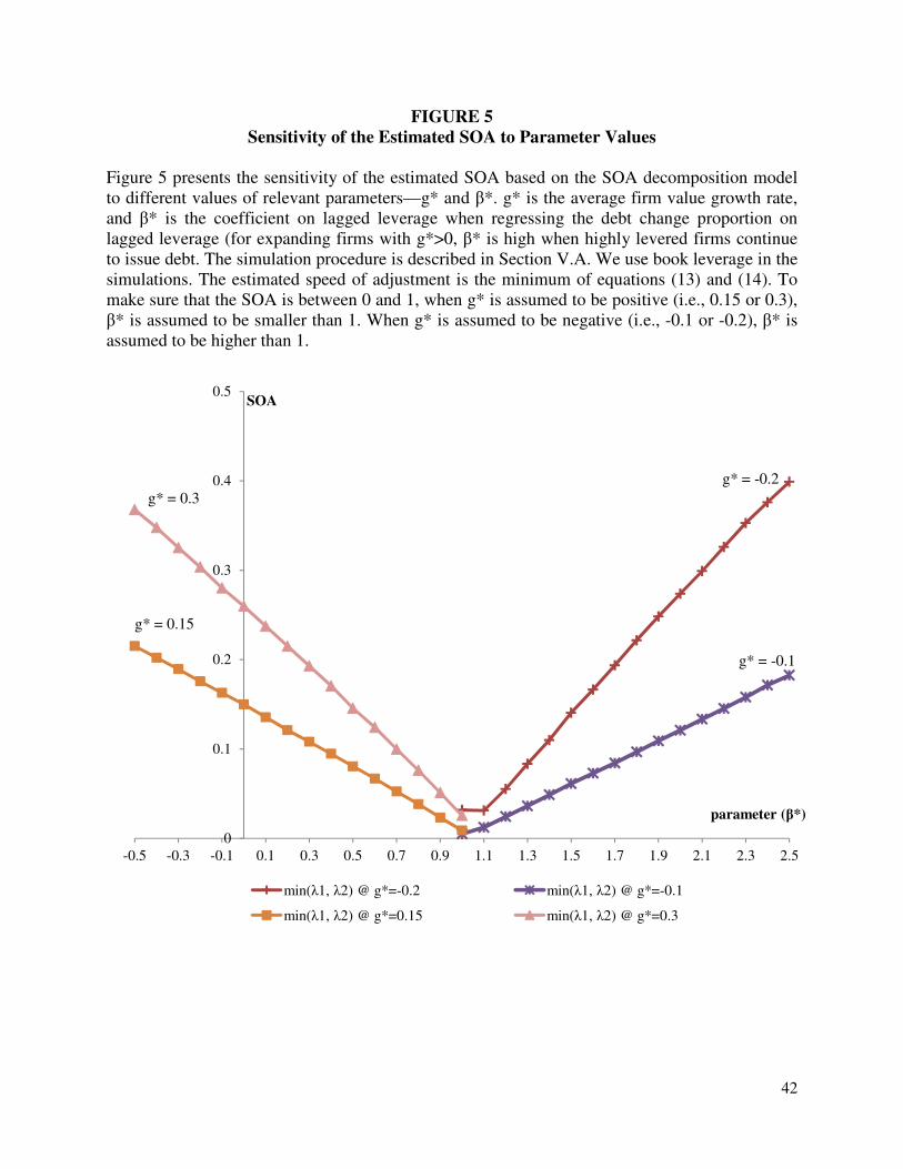
42

FIGURE 5

Sensitivity of the Estimated SOA to Parameter Values

Figure 5 presents the sensitivity of the estimated SOA based on the SOA decomposition model to different values of relevant parameters—g* and β*. g* is the average firm value growth rate, and β* is the coefficient on lagged leverage when regressing the debt change proportion on lagged leverage (for expanding firms with g*>0, β* is high when highly levered firms continue to issue debt. The simulation procedure is described in Section V.A. We use book leverage in the simulations. The estimated speed of adjustment is the minimum of equations (13) and (14). To make sure that the SOA is between 0 and 1, when g* is assumed to be positive (i.e., 0.15 or 0.3), β* is assumed to be smaller than 1. When g* is assumed to be negative (i.e., -0.1 or -0.2), β* is assumed to be higher than 1.

0

0.1

0.2

0.3

0.4

0.5

-0.5 -0.3 -0.1 0.1 0.3 0.5 0.7 0.9 1.1 1.3 1.5 1.7 1.9 2.1 2.3 2.5

SOA

parameter (β*)

min(λ1, λ2) @ g*=-0.2 min(λ1, λ2) @ g*=-0.1

min(λ1, λ2) @ g*=0.15 min(λ1, λ2) @ g*=0.3

g* = -0.1

g* = 0.15

g* = 0.3 g* = -0.2

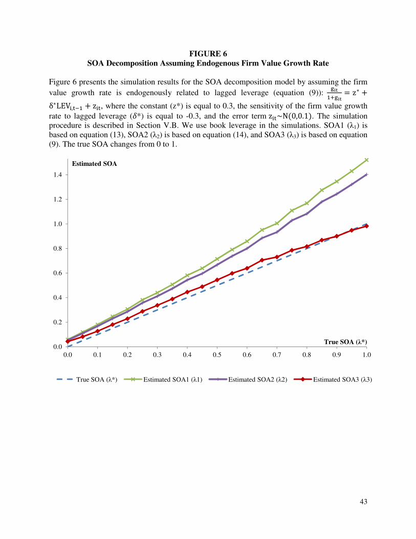
43

FIGURE 6

SOA Decomposition Assuming Endogenous Firm Value Growth Rate

Figure 6 presents the simulation results for the SOA decomposition model by assuming the firm

value growth rate is endogenously related to lagged leverage (equation (9)): -&'

�+-&'= z∗ +

δ∗LEV�,�� + z�, where the constant (z*) is equal to 0.3, the sensitivity of the firm value growth

rate to lagged leverage (R*) is equal to -0.3, and the error term z�~N(0,0.1). The simulation procedure is described in Section V.B. We use book leverage in the simulations. SOA1 (λ1) is based on equation (13), SOA2 (λ2) is based on equation (14), and SOA3 (λ3) is based on equation (9). The true SOA changes from 0 to 1.

0.0

0.2

0.4

0.6

0.8

1.0

1.2

1.4

0.0 0.1 0.2 0.3 0.4 0.5 0.6 0.7 0.8 0.9 1.0

Estimated SOA

True SOA (λ*)

True SOA (λ*) Estimated SOA1 (λ1) Estimated SOA2 (λ2) Estimated SOA3 (λ3)

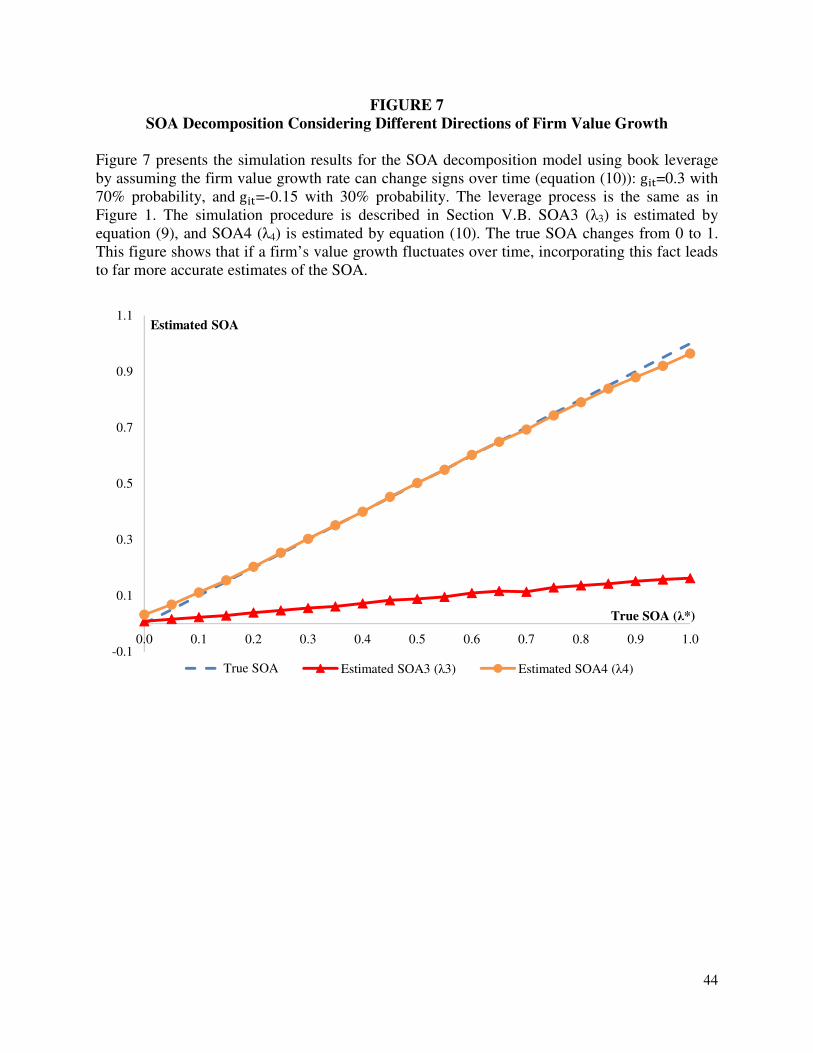
44

FIGURE 7

SOA Decomposition Considering Different Directions of Firm Value Growth

Figure 7 presents the simulation results for the SOA decomposition model using book leverage by assuming the firm value growth rate can change signs over time (equation (10)): g�=0.3 with 70% probability, and g�=-0.15 with 30% probability. The leverage process is the same as in Figure 1. The simulation procedure is described in Section V.B. SOA3 (λ3) is estimated by equation (9), and SOA4 (λ4) is estimated by equation (10). The true SOA changes from 0 to 1. This figure shows that if a firm’s value growth fluctuates over time, incorporating this fact leads to far more accurate estimates of the SOA.

-0.1

0.1

0.3

0.5

0.7

0.9

1.1

0.0 0.1 0.2 0.3 0.4 0.5 0.6 0.7 0.8 0.9 1.0

Estimated SOA

True SOA (λ*)

True SOA Estimated SOA3 (λ3) Estimated SOA4 (λ4)

45

FIGURE 8

SOA Decomposition With and Without Firm-Fixed Effects

Figure 8 presents the simulation results for the SOA decomposition model with and without firm-fixed effects in the leverage partial adjustment model (equation (12)). We assume that the firm value growth rate always has the same sign and has an average equal to 0.3. The simulation procedure is described in Section V.B. We use book leverage in the simulations. SOA1 (λ1) is estimated by equation (13), SOA2 (λ2) is estimated by equation (14), and SOA5 (λ5) is estimated by equation (12). The true SOA changes from 0 to 1.The figure shows that, for a true SOA of less than 0.5, including firm-fixed effects produces an estimated SOA that has a slight upward bias.

0.0

0.1

0.2

0.3

0.4

0.5

0.6

0.7

0.8

0.9

1.0

1.1

0.0 0.1 0.2 0.3 0.4 0.5 0.6 0.7 0.8 0.9 1.0

Estimated SOA

True SOA (λ*)

True SOA (λ*) min(λ1, λ2) [no FE] Estimated SOA5 (λ5) [with FE]

46

FIGURE 9

SOA Simulation Assuming that Firms Target Their Market Leverage Ratios

Figure 9 presents a similar analysis as in Figure 3, except that the simulated firms are assumed to target their market leverage ratios instead of book leverage ratios: Market leverage follows the partial adjustment model with firm-fixed effects (equation (11)) and a true market SOA of 0.3. The book and market SOAs that are plotted are estimated by equation (12), which includes firm-fixed effects and allows the firm value growth rate to change signs. η measures the additional noise (or standard deviation) in the market value growth process relative to the book assets growth process, and m denotes the ratio of the market value growth rate to the book assets growth rate on average, and can be interpreted as a marginal Tobin’s Q proxy. This figure shows that as the market value growth rate changes by a larger magnitude (larger m) or becomes more random (larger η) than the book assets growth rate, the estimated book SOA tends to get smaller relative to the estimated market SOA.

0.00

0.05

0.10

0.15

0.20

0.25

0.30

0.35

0.10 0.20 0.30 0.40 0.50 0.60

SOA

η

Book SOA @ m=1 Book SOA @ m=3Market SOA True Market SOA

47

TABLE 1

List of Papers Using a Dynamic Setting for Leverage

Among 42 empirical papers about capital structure published in five top-tier finance journals (Journal of Finance, Journal of Financial Economics, Review of Financial Studies, Journal of

Financial and Quantitative Analysis, and Financial Management) during 2014 to 2018, this table lists 16 of them that discuss the dynamic leverage adjustment model or the change in the leverage ratio. In these papers, the dependent variable is the leverage ratio or the change in the leverage ratio, and the independent variables include lagged leverage ratio. All of them use the book value debt ratio as a measure for leverage, and ten of them include results using the market value debt ratio.

Paper Include market

leverage? Relevant

tables/figures

Badoer & James (2016, JF) No Table 7 Baghai, Servaes, & Tamayo (2014, JF) No Table 6 Boubaker, Rouatbi, & Saffar (2017, FM) Yes Table 5 Brisker & Wang (2017, FM) Yes Table 5, Table 9 DeAngelo & Roll (2015, JF) Yes Figure 1 DeAngelo, Goncalves, & Stulz (2018, RFS) Yes Table 1 Elsas & Florysiak (2015, JFQA) Yes Table 9 Fu & Tang (2016, FM) No Not reported Halling, Yu, & Zechner (2016, JFE) Yes Table 3, Table 5 Ho, Huang, Lin, & Yen (2016, JFE) Yes Table 3, Table 4 Jiang, Jiang, Huang, Kim, & Nofsinger (2017, FM) No Table 2, Table 4 Leary & Roberts (2014, JF) Yes Table 4 Marciukaityte (2015, FM) Yes Table 4, Table 10 Oztekin (2015, JFQA) Yes Table 1 Phan (2014, JFQA) No Table 5 Walker, Yost, & Zhao (2016, FM) No Table 3, Table 4

48

TABLE 2

Summary Statistics

Table 2 presents the summary statistics of the sample firms extracted from the Compustat database. The sample includes non-financial and non-utility (i.e., excluding SIC within 6000-6999 and within 4900-4999) U.S. firms from 1965 to 2013, with at least 4 consecutive years of data, non-missing values of total assets, and positive values of book and market equity. It includes 124,512 firm-year observations for 9,170 distinct firms. Except for real total assets (1983 $), ln(real total assets), Tobin’s Q, the R&D dummy, and the rated dummy, all other variables are denoted as percentages. All variables are winsorized at their 1st and 99th percentiles prior to computing the numbers that are reported. For leverage, debt is defined to include all liabilities. Detailed definitions of all variables are as follows:

LEVB= book debt/total assets(AT), where book debt = total liabilities(LT)+preferred stocks(PSTKL)-deferred taxes(TXDITC)-convertible debt(DCVT). LEVM=book debt/(book debt+market equity), where market equity = stock price(PRC_F)*shares outstanding(CSHO). TOBINQ=(book debt+market equity)/total assets. EBIT = income before extraordinary items (IB)+interest expense (XINT)+income taxes (TXT) NET_PPE = net property, plant, and equipment (PPENT) RD_DUMMY = 1 if the firm does not report R&D expenses (XRD), and zero otherwises. RATED_DUMMY =1 if the firm has a public debt rating in Compustat, and zero otherwise. IND_MEDIAN_LEVB = median book leverage ratio based on Fama and French (2002) 49-industry classification, denoted in percentage IND_MEDIAN_LEVM = median market leverage ratio based on Fama and French (2002) 49-industry classification, denoted in percentage

Variable Mean Std Min Median Max

LEVB, % 45.78 20.79 5.66 45.34 97.94

LEVM, % 38.56 23.88 1.71 35.96 91.91

TOTAL_ASSETS, $m (1983 $) 797.01 2263.68 7.00 116.17 16360.47

Ln(TOTAL_ASSETS) 18.78 1.76 15.76 18.57 23.52

TOBINQ 1.63 1.19 0.54 1.24 7.73

EBIT/TOTAL_ASSETS, % 6.53 15.73 -71.82 9.13 36.14

NET_PPE/TOTAL_ASSETS, % 30.53 21.76 0.91 25.84 88.51

RD_DUMMY (no R&D expenses=1) 0.55 0.50 0.00 1.00 1.00

XRD/TOTAL_ASSETS, % 3.23 6.79 0.00 0.00 40.51

RATED_DUMMY 0.17 0.38 0.00 0.00 1.00

IND_MEDIAN_LEVB, % 43.87 8.76 21.47 45.09 61.29

IND_MEDIAN_LEVM, % 34.92 14.24 6.85 34.96 69.42

49

TABLE 3

Comparison of Firm Value Growth between Book and Market Value Measures

In Panel A, we compare the mean and variance of the annual book assets growth rate and the

market value growth rate. The book assets growth rate, g�l, is the annual change in total assets

scaled by lagged total assets, and the market value growth rate, g�k, is the annual change in the sum of book debt and market equity scaled by the sum of lagged book debt and lagged market equity. The book assets growth rate and market value growth rate are denoted in decimal format. In Panel B, we first divide firms into two groups according to the directions of book assets growth: a) book assets rise, and b) book assets fall. Then, conditioning on the direction of book assets growth, we further divide each group into three sub-groups based on the relative size of market value growth to book assets growth: 1) market value changes in the same direction but less than book assets; 2) market value changes in different direction with book assets; and 3) market value changes in the same direction but even more than book assets. Each cell shows the number of firms in that sub-group. The last row in each column presents the sum of groups a) and b) within that column. The numbers in square brackets are the percentage of firms in a given sub-group relative to total observations in that row.***, **, and * denote significance level at 1%, 5%, and 10%, respectively.

Panel A: Mean Comparison

Book assets growth

rate (g�l)

Market value growth

rate (g�k) Difference in mean

Mean 0.134 0.148 0.014*** Variance 0.099 0.218

# of obs 112,440 112,440

Panel B: Count of Firms by the Sign and Size of the Firm Value Growth Rate

1) Less change in

market value 2) Different directions

3) More change in market value

a) Rising book assets 18,728 22,939 38,425

[23%] [29%] [48%]

b) Falling book assets 5,833 9,991 16,524

[18%] [31%] [51%]

Sum: a)+b) 24,561 32,930 54,949 [22%] [29%] [49%]

50

TABLE 4

SOA Considering the Different Directions of Firm Value Growth

The bottom row shows the book and market SOA estimates (denoted as λ4) for the Compustat sample of 124,512 firm-years observations from 1965 to 2013 based on equation (10) that considers the different directions of firm value growth:

λ4=z1(1-β1)-w1δ1+δ1(1-β1)f(LEV)+adjustment terms,

where f�LEV�,�� = TE�LEV�,��U − E�LEV�,��� E�LEV�,�� V σ��⁄ , and “adjustment terms”

represents the three terms related to negative firm value growth. All parameters are estimated using OLS regressions without firm-fixed effects. Estimated book SOA (column 1) is calculated based on actual book leverage and actual book assets growth for the Compustat sample. Estimated Market SOA (column 2) is calculated based on actual market leverage and actual market value growth for the Compustat sample. Column 3 presents the market SOA by using the actual market leverage value and assuming that the firm value growth rate is equal to the book assets growth rate. In other words, column 3 estimates the market SOA under the assumption that there is no additional variation of the market value growth rate relative to the book assets growth rate.

Estimated Book SOA

Estimated Market

SOA

Market SOA if

g�k=g�l

w1 0.335

0.267

0.276 β1 0.038

0.162

0.215

z1 0.168

0.285

0.200 δ1 -0.034

-0.159

-0.134

f(LEV) 0.947

0.849

0.849 Adjustment terms -0.025

0.024

-0.025

Estimated SOA (λ4) 0.117 0.192 0.055

51

TABLE 5

Influence of Firm-Fixed Effects

Table 5 compares the influence of firm-fixed effects on the book and market SOA estimates for the Compustat sample. To estimate the size of firm-fixed effects, we first estimate the DPF model for book leverage as in Elsas and Florysiak (2015). Independent variables include lagged book leverage, Tobin’s Q, ln(real total assets), the ratio of EBIT to total assets, the ratio of fixed assets to total assets, R&D dummy, the ratio of R&D to total assets, rated dummy, median of industry book leverage, and firm fixed effects. After estimating the model, we sum up all the time-invariant components in the model that are related to the initial book leverage and within-firm averages of all the explanatory variables, and the summation would be equivalent to the firm-fixed effects term for book leverage (γB) as in equation (11). The firm-fixed effects term for market leverage (γM) is assumed to be the within-firm average of γB divided by Tobin’s Q. In Panel A, we calculate the standard deviation of the firm-fixed effects

term (σh, in percentage), the standard deviation of lagged leverage (σ�, in percentage), and the

ratio between these two standard deviations (σh /σ� , in decimal), based on book value

measures and market value measures, respectively. In Panel B, we adjust the estimated SOA in Panel B of Table 4 by adding the firm-fixed effects correction term using equation (12), denoted as λ5:

λy = �� �λx + dλx� + 4σh� σ��⁄ �,

where λx is the estimated SOA in Table 4 using OLS regressions. In both panels, column 1 and column 2 are the estimates based on the actual book value and market value. Column 3 shows the implied market estimate based on the actual market leverage process but assumes that the firm value growth rate is equal to the book assets growth rate and the firm-heterogeneity term (γ) is the same as book leverage distribution.

Panel A: Size of Firm-Fixed Effects

Book

Estimate Market

Estimate Market Estimate if gM=gB

and γM=γB

σh, % 1.702 3.049 1.702

σ�, % 20.249 23.532 23.532

σh σ�⁄ 0.084 0.130 0.072

Panel B: SOA with Firm-Fixed Effects

λ4 (in Table 4) 0.117 0.192 0.055 λy (adjusted for firm-fixed effects) 0.161 0.257 0.105

52

TABLE 6

The Coefficient β and Different Capital Structure Theories

Table 6 summarizes the expected sign or value of the coefficient β, defined in Proposition 1,

which is the slope of the regression of the net debt proportion on lagged leverage, based on

different capital structure theories. The expression for β is Cov�d� g�⁄ , LEV�,�� σ����⁄ ), where

d� is the net debt change scaled by lagged total assets, g� is the change of total assets scaled by

lagged total assets, and Lev�,�� is lagged leverage. Considering that most firms are expanding in

the real world, we mainly focus on the case of a positive firm value growth rate, g.

Theory

Implication about the relationship between the net debt issuance proportion and lagged leverage (the coefficient β)

Trade off

Highly levered firms are more likely to be over-levered, and hence are less likely to issue debt. � β<0.

Market timing Firms are more likely to issue equity when equity is overvalued.

Overvalued equity tends to result in low leverage. So low levered firms are less likely to issue debt. � β>0.

Pecking order Firms prefer internal funds to debt and then to equity. Debt issuance

depends on cash shortage rather than lagged leverage. � β=0. If urgent external financing is positively correlated lagged leverage, β>0 when debt can be issued, and β<0 when money-losing firms have to issue equity.

Random financing Firms randomly choose to issue debt or equity, and hence debt issuance is

unrelated to lagged leverage. � β=0, and debt issuance also has no correlation with any economic factors such as the shortage of internal funds.