THE STABILITY OF MONEY DEMAND IN CROATIA IN

1149

UDK 332.4:332.5(495.7)

Izvorni znanstveni rad

THE STABILITY OF MONEY DEMAND IN CROATIA

IN POSTSTABILIZATION PERIOD

Autori u članku procjenjuju funkciju potražnje za novcem u Hrvatskoj zanovčane agregate M1 i M1a unutar vektorske autoregresije. Potražnja zanovčanim saldom se povećala nakon uvođenja antiinflacijskog stabilizacijskogprograma godine 1993. Monetarnu politiku je ograničila liberalizacija deviz-nog tržišta i deviznog tečaja, očekivana inflacija je bila smanjena, a kućanstvasu zamijenila ukinutu deviznu štednju domaćom valutom. Rezultat toga je biopromjena u potražnji za novcem.

Introduction

Analysing demand for money in Croatia is important for several reasons:(a) The money demand function in Croatia will be estimated for two mone-

tary aggregates within small vector autoregression (VAR)1. That means that wetake in account simultaneity of the included variables to ensure efficient estima-tion of the long-run coefficients of the model.

(b) Demand for money balances was increased after introducing anti-infla-tion stabilization program on October 4, 1993 by the Croatian government. Na-mely, monetary policy was restrictive with liberalization of foreign exchange mar-ket and exhange rate. Expected inflation was reduced (with appreciation of thenominal and real exhange rate). Housholds replaced their foreign exchange sa-vings with domestic currency and the result was change in the money demand.

* N. Erjavec, docent Ekonomskog fakulteta Sveučilišta u Zagrebu. B. Cota, docent Ekonomskogfakulteta Sveučilišta u Zagrebu. Članak primljen u uredništvu: 05. 06. 2001.

1Analysing monetary aggregate M4 does not lead to sensible outcomes. Diagnostic statisticsof the chosen model are very poor and not acceptable. That is why we exclude that aggregate fromthe analysis. We hope that longer available data series might improve the analysis.

Nataša Erjavec and Boris Cota*

N. ERJAVEC, B. COTA: The Stability of money demand in Croatia in poststabilization periodEKONOMSKI PREGLED, 52 (9-10) 1149-1172 (2001)1150

(c) It is interesting to look in detail at the stability of the money demand fun-ction in a small country which is, and will be, mostly dependent on European mo-netary union. Some papers show that European money demand function has grea-ter stability compared to most estimates on national level (see Artis et al. 1993,Hayo, 1999).

The goal of this paper is to provide estimates of real money demand overpoststabilization period. This is not a complement to the previous work on esti-mation of the demand for real money balances in Croatia (Anušić 1994; Anušićet.al. 1995, Babić, 1998, Payne, 2000) because we undertake more advanced eco-nometric approach i.e. cointegration methodology. This paper can be viewed assome kind of further research and a complement to the estimation transactory de-mand for money (Babić, 2000).

Data and Methodology

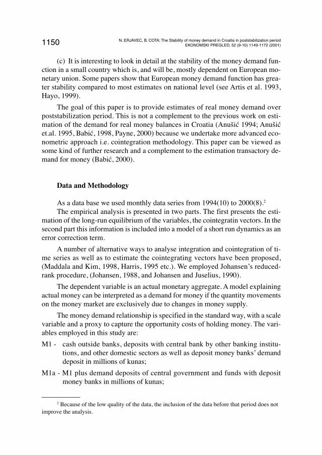
As a data base we used monthly data series from 1994(10) to 2000(8).2

The empirical analysis is presented in two parts. The first presents the esti-mation of the long-run equilibrium of the variables, the cointegratin vectors. In thesecond part this information is included into a model of a short run dynamics as anerror correction term.

A number of alternative ways to analyse integration and cointegration of ti-me series as well as to estimate the cointegrating vectors have been proposed,(Maddala and Kim, 1998, Harris, 1995 etc.). We employed Johansen’s reduced-rank procedure, (Johansen, 1988, and Johansen and Juselius, 1990).

The dependent variable is an actual monetary aggregate. A model explainingactual money can be interpreted as a demand for money if the quantity movementson the money market are exclusively due to changes in money supply.

The money demand relationship is specified in the standard way, with a scalevariable and a proxy to capture the opportunity costs of holding money. The vari-ables employed in this study are:

M1 - cash outside banks, deposits with central bank by other banking institu-tions, and other domestic sectors as well as deposit money banks’ demanddeposit in millions of kunas;

M1a - M1 plus demand deposits of central government and funds with depositmoney banks in millions of kunas;

2 Because of the low quality of the data, the inclusion of the data before that period does notimprove the analysis.

1151N. ERJAVEC, B. COTA: The Stability of money demand in Croatia in poststabilization periodEKONOMSKI PREGLED, 52 (9-10) 1149-1172 (2001)

M4 - M1 plus savings and time deposits, foreign currency deposits as well asbonds and money market instruments;CPI- retail price index, base 1998=100;GDP- collected revenues of the economy as a whole andINT- deposit money banks’ interest rates on deposit in kunas, average.3

Money and income variables are in logarithms. All variables are seasonallyunadjusted. In a view of the theoretical and empirical evidence we estimated thedemand for real money; i.e. we imposed price homogeneity. The results of moneydemand studies are robust with respect to the choice of the deflator so CPI hasbeen chosen as a deflator for the income and money variables.

Before testing for cointegration, the order of integration of the individual ti-me-series must be determined. Tests for unit roots were performed on all of thedata using ADF test (Dickey-Fuller, 1979) and KPSS test (Kwiatkowski, Phillips,Schmidt and Shin 1992). The difference between these two tests is in the formu-lation of the null hypothesis. ADF test has a nonstationarity as a null hypothesisi.e. the null hypothesis is that the variable under investigation has a unit root. Onthe other hand, in the KPSS test we assume that the variable is stationary. It hasbeen suggested (KPSS, 1992) that the tests using stationarity as a null can be usedfor confirmatory analysis, i.e. to confirm our conclusion about unit root tests. Ifboth tests fail to reject the respective nulls or both reject the respective nulls, wedo have a confirmation4. The resultes5 are reported in Table 1. The variables usedin this study are given in the first column of Table 1. The top part of table reportstests of stationarity of the log-levels6 of the variables and the bottom half of theirfirst differences. Columns two and three contain test values for ADF tests with theinformation about use of a constant term or a deterministic trend. The strategy ofadding lags to the ADF regression is based on the objective to remove anyautocorrelation from the residuals, which is tested applying Lagrange Multipliertest.

3 Collected revenues of the economy as a whole is proxy for gross domestic product on amonthly bases. Data on gross domestic product can be obtained only as a quarterly and annual esti-mations. Retail price index is a measure of changes in retail prices of goods and services and it isused as a measure of inflation.

4 The situation is similar to the tests of nontested hypotheses.5 All empirical work was performed with RATS and CATS statistical packages of Doan

(1992).6 Letter L denotes log-transformation.


Table 1

VARIABLES AND UNIT ROOT TESTS

(a) Lavels

Variable ADF value ADF value KPSS value KPSS valueConstant Constant and H

0 stationary H

0 trend

included trend included around a level stationary

LM1 -1,6262(13) -2,3141(12) 0,51822* 0,16580*

LM1a -1,5218(13) -2,5722(13) 0,51627* 0,15585*

LGDP -2,0451(3) -2,3695(15) 0,79601** 0,08888

INT -0,6199(0) -2,0613(0) 4,01508** 0,34440**

LCPI 1,3650(0) -2,1577(0) 7,02585** 0,96301**

(b) First Differences

First diff. ADF value ADF value KPPS value KPPS valueConstant Constant and H

0 stationary H

0 trend

included trend included around a level stationary

∆LM1 -7,1740** (1) -2,9264(4) 0,34082 0,13515

∆LM1a -1,0718(12) -7,0922** (1) 0,33770 0,13385

∆LGDP -31,1538**(0) -3,3002(5) 0,29234 0,13666

∆INT -22,2780** (0) -21,8332** (0) 0,43038 0,16079

∆LCPI -932,6942** (0) -919,9228** (0) 0,32702 0,13230

Notes: ∆ is the first difference operator. One (two) asterisk(s) indicates a rejaction of theNull at 5% (1%) significance level. The critical values for ADF test are taken fromHamilton (1994) and for KPSS test from KPSS (1992).

The appropriate number of lagged differences is determined by adding lagsuntil a LM test fails to reject no serial correlation of order 12 at 5% level. In squarebrackets after the test values, the length of included lags is given. In the fourthcolumn the KPSS test values, testing stationarity around level are given and in thefifth KPSS test values testing trend stationarity of the variables.

As can be seen from Table 1, variables appear to be integrated of order one,i.e. being I(1), although some of the results are sensitive to the number of includedlags. Generally the resultes of KPSS tests confirm the resultes of ADF tests. So inthe remainder of this study all variables are treated as being I(1).


In this paper we analysed a simple model of a demand for money. The ge-neral theoretical long-run relationship is specified as (Hayo, 2000):

(1)

Including variable ∆LCPI, i.e. inflation rate, as additional opportunity costvariable into the cointegrating vector did not lead to sensible outcomes. It is ob-vious because of relatively stable price level over the post-stabilization period.But it does appear to play a role in the short-run dynamics of M1a. Since we usereal variables in the model, inflation should not affect money demand in a perfectworld. However rigidities in the real world means that the inflation rate may helpus to explain money growth.7

Because our primar interest was to study short- and long- term stability of themoney demand function we did not include additional variables in the model, likeother interest rates.8

The empirical estimates for the monetary aggregates are given in the nextsection. First we analyse the money demand function for M1.

Modeling the Demand for M1

The cointegration analysis starts with the following unrestricted VAR model:

(2)

where: Zt = (LM1, LGDP, INT)’, Ψ and Γ

i are matrices of parameters. β is 3 by r

matrix of cointegration vectors, α is 3 by r matrix of the respective loadings ofcointegrating vectors. r is a number of cointegrating vectors of the system, D

t is a

vector of non-stochastic variables: seasonals, constant and dummy variables. ut is

a vector of residuals of the system and k is a lag length of the VAR model.

A descriptive analysis of the variable INT shows that there is a shift in theseries taken place from 1996(6) to 1996(12). This property can be explained byrehabilitation of the two largest regional banks (Riječka banka and Splitska ban-

M

P

GDP

PINT

t t

t

⎛⎝⎜

⎞⎠⎟

=⎛⎝⎜

⎞⎠⎟

( )β

β11

12exp

7 Inflation may be a proxy for the yield of real assets. So changes in real assets will influencethe decision to hold money if real assets are important in investor’s portfolios. M1a contains moneycomponents that are more subject to portfolio decision.

8 If we were interested to maximize the fit of the model, we should have included additionalvariables.

∆ Γ ∆ ΨZ Z Z D ut i

i

k

t t t t= + ′ + +=

−

− −∑1

1

1 1αβ


ka) so we included a step dummy variable D6a12y96 in the system9. During ana-lysed period there were also some events that might affect the relationship bet-ween real money and real income in the Republic of Croatia. Introducing the Va-lue Added Taxes (VAT) at the beginning of 1998 and police and military actionsduring the war appear to have caused structural breaks in the series. So we addi-tionaly added dummy variables PDV, TB and “Oluja” to neutralise those effects10.

In Table 2 we present the results of estimating and testing for the number ofcointegrating vectors using a VAR containing four lags of the variable in lavels.

For the Johansen procedure, there are two test statististics for the number ofcointegrating vectors: the trace (λ

trace) and the maximum value statististics, (λ

max).

In the trace test, the null hypothesis is that the number of cointegrating vectors isless than or equal to r, where r = 0 to 3. In each case the null hypothesisis is testedagainest the general alternative. The maximum eigenvalue test is similar, exceptthat alternative hypothesis is explicit. The null hypotheisis r=0 is tested against thealternative that r=1, r=1 againest r=2 etc.

Table 2

ESTIMATING AND TESTING THE COINTEGRATING VECTORS FOR LM1

H0: r = p-r λ

max λ

trace λ

0 3 36,14** 49,34** 0,4169

1 2 12,92 13,20 0,1753

2 1 0,28 0,28 0,0042

BETA (transposed)

LM1 LGDP INT CONSTANT

1.000 -0.792 0.009 -5.981

Loading of α̂11

= -0,129

Note: ‘**’ Indicates a rejection of the Null at 1% and ‘*’ at 5 % significance level. The cri-tical values are taken from Osterwald-Lenum, (1992) and are only indicative becau-se of the dummy variables.

9 D6a12y96=1 if 1996 (6) ≤ t ≤ 1996 (12), 0 otherwise.10 PDV is a dummy variable defined: PDV=1 for t ≤ 1998 (1) and 0 otherwise, which is intro-

duced to neutralize the permenant effects of introducing the VAT in Croatia at the beginning of 1998.TB is a pulse function defined TB=1 if t=1998(1), 0 otherwise added to the system to neutralize thetransitory effects of introducing a VAT. “Oluja” is a dummy variable defined OLUJA=1 if 1995 (5) ≤t ≤ 1995 (8), 0 otherwise to neutralize the effects of police and military actions “Bljesak” and“Oluja”.


From the resultes in Table 2 we can conclude that there exists one significantcointegrating vector, β̂

1. The relevant adjustement parameter of the loading vector

α̂11

is not small, (-0.129). This implies that a deviation from the long-run equili-brium exert pressure on money growth. The diagnostic statistics of this estimatedo not indicate any statistical problems. Residual analysis of the whole system aswell as of the each variable included in the system is also acceptable11.

The income elasticity of money demand as estimated by β̂1vector is nearly

one. On the other hand, the interest rate enters the cointegration relationship with atheoreticaly consistent sign and its apsolute effect is small. Using our findings ofone cointegrating vector, we computed an appropriate LR- test for testing the res-triction that the income elastisity is unity and the interest rate semi-elasticity iszero. The obtained resultes are presented in Table 3.

Table 3

TESTING RESTRICTIONS ON COINTEGRATING AND ADJUSTMENTVECTORS FOR LM1

Restrictions on β̂1’ = (1,-1,0) β̂

1’=(1,-1,0) β̂

1’=(1,-1,0) β̂

1’=(1,-1,0)

β̂1’

Restrictions on α̂1 unrestricted α̂

1 =(u,0,0) α̂

1 =(u,u,0) α̂

1 =(u,0,u)

α̂

Test statistics χ 2 (2) = 0,34 χ 2 (4) = 1,34 χ 2 (3) = 0,54 χ 2 (3) = 0,98

p-value 0,84 0,86 0,91 0,81

The resulting restricted estimate of the long-run relationship can be called aclassical version of money demand, as it is computed with constraints β

11 = 1 and

β12

imposed on the equation (1). Moreover, additional tests (not included here)show that dummy variables included in the cointegration space are not significant.We continue by keeping these restriction on the cointegrating vector and test forweak exogeneity of the adjusting parameters associated with the income and in-terest rate variable.

11 We reject the hypothesis of the autocorrelation of residuals, for each variable and for a wholesystem, but there is a violation of the assumption of normality. We believe that it is due to INT vari-able. Following Johansen and Juselius (1992), non-normality in the individual variable is not such aproblem, because if that variable prove to be weakly exogenous, in further analysis we can conditionon it (although it remains in a long-run model) and therefore improve the stochastic properties of themodel. This agrees with our results further on.


Performing likelihood ratio tests of the adjustment parameters involving theeigenvalues of the system, we accept the null of weak exogeneity for both GDPand INT jointly (column 3) as well as testing them independently (columns 4 and5). Accordingly, further on we do not analyse a money demand in a system con-test, but through single equation model.

We continue the analysis with imposed restrictions on the weak exogenety ofincome and interest rate variables with the corresponding error correction termECMLM1 which is now calculated as:

ECMLM1=LM1 - LGDP - 4,990. (3)

The next step is to estimate the dynamic error correction model. The moneydemand equation consists of the first differences of the variable LM1, LGDP, INTand LCPI, cointegrating vector as a lagged error correction term, seasonal dum-mies and dummy variables12. Diagnostic statistics of the model are given in Table4.

Table 4

RESIDUAL ANALYSIS13 OF THE FINAL MODEL FOR LM1

TEST FOR AUTOCORRELATION TEST FOR NORMALITY

L-B(16), CHISQ(12)=23,035, p-val = 0.03 CHISQ(2) = 5,168, p-val = 0.08

LM(1), CHISQ(1)=0.162, p-val = 0.69

LM(4), CHISQ(1)=0.002, p-val = 0.97 ARCH(4) = 1.924

As it can be seen, the test statistics indicate model adequacy and we can con-clude that the final model is statisticaly acceptable. In Table 5 actual estimates ofthe ∆LM1 equation is pressented which can be interpreted as a dynamic moneydemand function. As we can see the error correction term has a significant and

12 Variables LGDP and INT are weakly exogenous and are included in the cointegration spaceas well as in the short-run dynamics. Variable LCPI is weakly exogenous included in the short-rundynamics but is excluded from the cointegration space. Dummy variables TB and “Oluja” were notsignificant and were excluded from the further analysis.

13 L-B is Ljung-Box test for residual autocorrelation based on the estimated auto- and cros-scorrelation on the first (T/4) lags, (Ljung and Box, 1978). LM(1) and LM(4) are LM- type tests forthe first and the fourth order autocorrelation (Godfrey, 1988). The test for normality is Shenton-Bowman test, (Doornik and Hansen, 1994). ARCH is a test for AutoRegressive Conditional Hetero-scedasticity, (Engle, 1982).


negative influence on the growth of real money. Thus we can conclude that it notonly has a statistically significant influence but, judging from the parameter size,it is also significant from the economic point of view. The parameter on the errorcorection term indicates an overall impact of 10,9% adjustment every month.

Table 5

ESTIMATION OF ∆LM1 EQUATION

Variable Coefficient “t-value”

∆LM1t-2

-0,308 -2,658

∆LM1t-3

-0,297 -2,932

∆LGDPt

0,097 3,087

∆INTt

-0,031 -2,669

∆INTt-1

-0,055 -4,320

∆INTt-3

-0,064 -4,495

ECMLM1t-1

-0,109 -6,264

D6a12y96 -0,040 -3,400

PDV -0,020 -4,358

The income variable has a positive influence on money growth, which is inaccordance with economic theory. While we found that in the long-run money de-mand appears to be of a classical type in the error correction model there exists asignificant negative effect of interest rate changes, in the actual period and withone and three months lag, on money growth. The influence is more pronounced inthe period three lags apart from the actual value, almost doubled in size. Thisshows the importance of opportunity cost effects for the demand for narrow mo-ney in the short-run. Apart from some money growth lags we find that dummyvariables D6a12y96 and PDV are significant. Because the series are not seaso-nally adjusted, some seasonal dummies are significant, too.

To check the stability of the final one-equation model and constancy of β weperformed a sequence of statistical tests. We chose a sub-sample from 1995(1) to1999(1) as a base period. When testing the constancy of β, the parameter β̂ is firstcalculated for the base period. The constancy of the cointegrating space is thentested using a sequence of tests of the “known vector” β, where the known vectoris represented by chosen β̂, sub-sample estimate have β.

First we perform the Trace test. When analysing the Trace statistic, Figure 1,one would expect the time path of Trace statistic to be upward sloping for j ≤ r,


and constant for j ≤ r. Since our conditional model has rank 1, we expect the timepath of Trace statistic to be upward sloping. Although it seems to be some changesby the end of the series, the general impression is that the time path is indeed up-ward sloping.

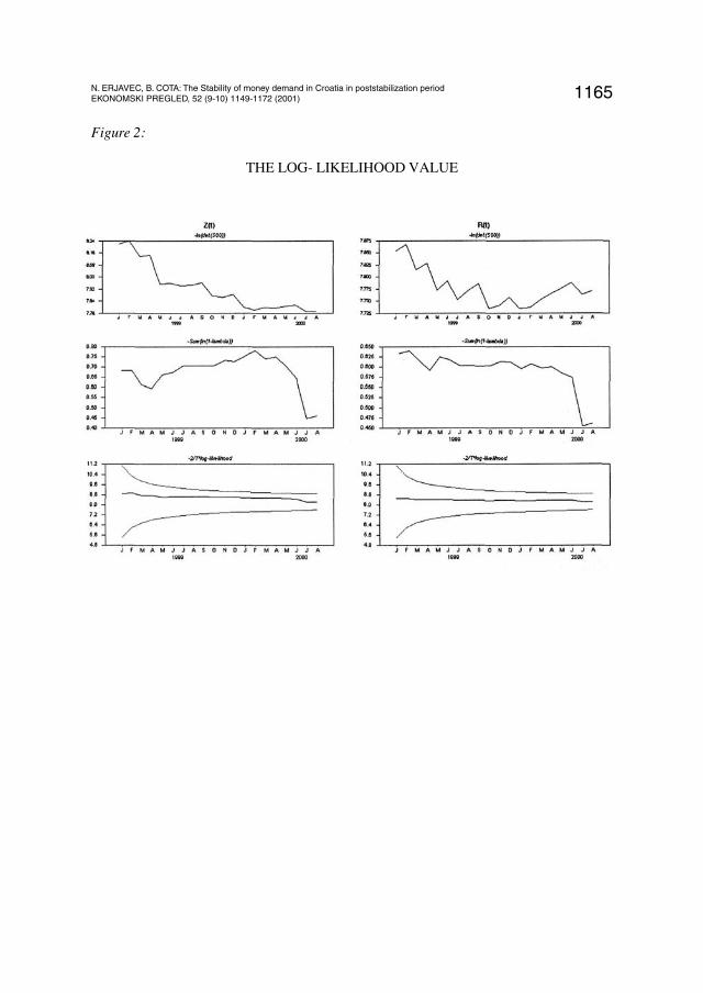
The maximised log-likelihood function, which consists of two factors, is gi-ven in Figure 2. The paths of two components look non-constant, but it is mainlydue to scaling of the graphs. The path for the log-likelihood value is well inside the95% confidence bounds for the full sample.

Figure 3 shows tests of the hypothesis that the full sample estimate of β withthe over-identifying restrictions imposed is in the space spanned by β in each sub-sample. The hypothesis is accepted. This supports the hypothesis of parameterconstancy for the analysed period.

Figure 4 gives plot of the time path of the non-zero eigenvalue together withthe asymptotic 95% error bounds for a sub-sample. As can be seen from Figure 4,the plot does not indicate non-constancy in our model.

Figure 5 presents various plots associated with diagnostic testing of the resi-duals. There are some evidence to suggest that there is a problem around 2000:6.It is not surprising because central government repayed loans to private sector anddeposit money increased. This results with some temporary fluctuations, but notwith a permanent structural break.

At the end, we can conclude that the final model is generally satisfactory,being a well interpretable and statistically acceptable money demand function.

Modeling the Demand for M1a

The same modelling procedure is applied to the monetary aggregate M1a.The resultes of the cointegration analysis in a VAR with four lags are given in Ta-ble 6.


Table 6.

ESTIMATING AND TESTING THE COINTEGRATING VECTORS FOR LM1a

H0: r = p-r λ

max λ

trace λ

0 3 30,70** 44,47** 0,3676

1 2 13,49 13,77 0,1824

2 1 0,28 0,28 0,0042

BETA (transposed)

LM1 LGDP INT CONSTANT

1.000 -0.785 0.002 -5.970

Loading of α̂11

= -0.130

Note: ‘**’ indicates a rejection of the Null at 1% and ‘*’ at 5 % significance level. Thecritical values are taken from Osterwald-Lenum, (1992) and are only indicative be-cause of the dummy variables.

As in the case with money aggregate M1 only one significant vector is found.Compared to narrow money, the estimates of the long-run equilibrium are almostthe same. Again the diagnostic tests are acceptable and do not indicate any modelnon-adequancy. Testing the restrictions on the adjustment and cointegrating vectorwe obtained the results in Table 7.

Table 7

TESTING RESTRICTIONS ON COINTEGRATING AND ADJUSTMENTVECTORS FOR LM1a

Restrictions on β̂1’ = (1,-1,0) β̂

1’=(1,-1,0) β̂

1’=(1,-1,0) β̂

1’=(1,-1,0)

β̂1’

Restrictions on α̂1 unrestricted α̂

1 =(u,0,0) α̂

1 =(u,u,0) α̂

1 =(u,0,u)

α̂1

Test statistics χ 2 (2) = 0,46 χ 2 (4) = 1,67 χ 2 (3) = 0,63 χ 2 (3) = 1,31

p-value 0,80 0,80 089 0,73

Because of the weak exogeneity of both GDP and INT we have to specifyone-equation model. Moreover, the unity restriction on the income elasticity of


money demand as well as interest rate semi-elasticity are accepted again. The fol-lowin error correction term will be included in the model when analysing LM1a.

ECMLM1a=LM1a - LGDP - 4,946 (4)

None of the test statistics, Table 8, indicates a problem and the final modelis statistically acceptable.

Table 8

RESIDUAL ANALYSIS OF THE FINAL MODEL FOR LM1a

TEST FOR AUTOCORRELATION TEST FOR NORMALITY

L-B(16), CHISQ(12)=17,132, p-val = 0.14 CHISQ(2) = 1.078, p-val = 0.56

LM(1), CHISQ(1)=0.028, p-val = 0.87

LM(4), CHISQ(1)=0.098, p-val = 0.76 ARCH(4) = 6.570

The actual estimates of the ∆LM1a equation is presented in Table 9. Again itcan be seen that the income variable has a positive influence on money growth andthat influence is a little bit stronger compared to the case of ∆LM1. The interestrate effects are negative and the values are very simmilar to the case of ∆LM1 mo-ney aggregate. Error correction term has the expected negative size and is statisti-caly significant. The size of the adjustment parameter is now a little bit bigger thenin the case of narrow money, so a long-run disequilibrium influence the short-runbehaviour of money growth more. Inflation is not present in the model with po-sitive impact on the money. It is represented by ∆LCPI variable. The same dummyvariables are significant and their influence, the values of the parameters, are al-most the same as in the case of narrow money. Some of the seasonals are signifi-cant, too.


Table 9

ESTIMATION OF ∆LM1a EQUATION

Variable Coefficient “t-value”

∆LM1at-1

-0,237 -2,155

∆LM1at-2

-0,423 -3,371

∆LM1at-3

-0,267 -2,313

∆LGDPt

0,115 3,474

∆INTt

-0,027 -2,176

∆INTt-1

-0,063 -4,700

∆INTt-3

-0,062 -4,216

∆LCPIt

-1,916 -2,413

ECMLM1t-1

-0,128 -5,824

D6a12y96 -0,047 -3,778

PDV -0,024 -4,357

The parameters constancy is tested through the recursive estimation.

Although it seems to be some changes by the end of the series, as in the caseof narrow money, the general impression is that time path is upward sloping andwithin the critical region.

The path of the log-likelihood value is well inside the 95% confidence bo-unds for the full sample, Figure 7. The test for constancy of the cointegration spa-ce, Figure 8, supports the hypothesis of parameter constancy for the analysed pe-riod.

The time path of the non-zero eigenvalue is well inside the asymptotic 95%error bounds for a sub-sample, which indicates constancy of the parameters in thepartial model.

Apart from the autocorrelation at lag=12, the diagnostic tests of the residualsseem to be generally satisfactory.

Conclusion

The demand for money is treated as demand for real balances. That meansthat the function is homogenous of degree one in the level of prices. Monetaryaggregates M1 and M1a show very similar behaviour during the analysed pe-riod.


We found, in accordance with economic theory, stable long-run and short--run money demand functions. Money demand appears to be of a classical type inthe long run; dominated by economic transactions. The estimated long-run inte-rest rate elasticity for M1 and M1a is zero and income elasticity is unity.

The corresponding error-correction term is an important explanatory vari-able in the short-run M1 and M1a demand functions. Therefore a disequlibrium inthe long-run relationship makes pressure on real money growth. That lies in a factthat the demand for money is transaction one. In the error correction model thereexists a significant and negative effect of interest rate changes on money growth(with one and three months lags). That shows the importance of opportunity costeffects for the demand for narow money and M1a in the short run.

Considering the statistical properties of the estimated models, apart from so-me outliers located at the end of the series, we found no serious evidence of mis-specification. There is the evidence that the D6a12y96 and introducing the ValueAdded Taxes (VAT) at the beginning of 1998 have statistically significant influ-ence on the short-run money demand functions, although their influence, accor-ding to parameter size, is not large. Police and military actions during the war ap-pear not to have any effects.

On the basis of the presented results we can not conclude that monetary poli-cy instruments cause money demand to shift (the parameter values of the corres-ponding variables are not large), so our opinion is that those instruments have be-come more market oriented.

LITERATURA:

1. Anušić, Z.: “The Determinants of Money Demand in Croatia and Simulation of Post- Stabilization Period”, Croatian Economic Survey, Insitute of Economics, Zagreband National Bank of Croatia, 1995.

2. Anušić, Z., Z. Rohatinski and V. Šonje (eds.): “A Road to Low Inflation: Croatia1993-1994”, The Government of the Republic of Croatia.

3. Artis, M. J., R. C. Bladen-Hovell and W. Zhang: “A European Money Demand Func-tion”, in P. R. Masson and M. P. Taylor (eds.), “Policy Issues in the Operation ofCurrency Unions”, Cambridge: Cambridge University Press, 1993., str. 240-263.

4. Babić, A.: “Stopping Hyperinflation in Croatia 1993-1994”, Zagreb Journal of Eco-nomics 2(2), 1998., str. 71-114.

5. Babić, A.: “The monthly Transaction Money Demand in Croatia”, Working Papers,W-5, Croatian National Bank, 2000.

6. Bulletin National Bank of Croatia, various numbers.


7. Dickey, D. A. and W. A. and Fuller: “Distributions of the estimators for autoregres-sive time series with unit root”, Journal of the American Statistical Association, 74,1979., str. 427-431.

8. Doan, A. T.: “User’s Manual: RATS”, Version 4.2., 1992.

9. Doornik, J. A. and Hansen, H.: “An omnibus test for univariate and multivariate nor-mality”, Working paper, Nuffield Collage, Oxford, 1994.

10. Engle, R.: “Autoregressive Conditional Heteroscedasticity with Estimates of the Va-riance of United Kingdom Inflation”, Econometrica, 38, 1982., str. 507-516.

11. Godfrey, L. G.: “Misspecification tests in econometrics. The Lagrange Multiplierprinciple and other approaches”, Cambridge University Press, 1988.

12. Hayo, B.: “The Demand for money in Austria”, Empirical Economics, Vol 25 (4),2000., str. 581-603.

13. Hayo, B.: “Estimating a European Demand for Money”, Scottish Journal of PoliticalEconomy, 46(3), 1999., str. 221-244.

14. Harris, R. I. D.: “Using Cointegration Analysis in Econometric Modeling”, PrenticeHall, London, 1995.

15. Hamilton, J. D.: “Time series analysis, Princeton, 1994.

16. Ljung and Box, G.: “On a measure of Lack of Fit in Time Series Models”, Biomet-rika, 65, 1978., str. 297-303.

17. Johansen, S.: “Statistical Analysis of Cointegration Vectors, Journal of EconomicDynamics and Control, Vol. 12, 1988., str. 231-54.

18. Johansen, S. and K. Juselius: “Maximum likelihood Estimation and Inference onCointegration - with Application to the Demand for Money”, Oxford Bulletin ofEconomics and Statistic, 52, 1990., str. 211-244.

19. Kwiatkowski D. , P.C.B. Phillips, P. Schmidt and Y. Shin: “Testing the Null Hypo-thesis of Stationary against the Alternative of a Unit Root”, Journal of Econometrics,54, 1992., str. 159-178.

20. Maddala G. S. and In-Moo Kim: “Unit Roots, Cointegration and Structural Chan-ge”, Cambridge University Press, Cambridge, 1998.

21. Osterwald-Lenum, M.: “A Not with Fractiles of the Asymptotic Distribution of theMaximum Likelihood Cointegration Rank Test Statistic, Oxford Bulletin of Econo-mics and Statistic, 54, 1992., str. 461-472.

22. Payne, J. E.: “Post Stabilization Estimates of Money Demand in Croatia: The role ofthe Exchange rate and Currency Substitution”, Ekonomski pregled, 11-12, 2000., str.1352-1368.


14 The Trace statistic is scaled by the 90% quantile of the trace distribution derived for a modelwithout exogenous variables or dummies. Asymptotic distribution is different if we are not analysinga standard model, which is the case here, so the lines of critical values are not valid. But our primaryinterest is in the time path of the statistic and the visual inspection of it is not affected by scaling.

Figure 1:

Plot of the Trace Statistic14


Figure 2:

THE LOG- LIKELIHOOD VALUE


Figure 3:

TEST OF CONSTANCY OF β̂

Figure 4:

THE NON-ZERO EIGENVALUE


Figure 5:

RESIDUAL ANALYSIS FOR LM1


Figure 6:

PLOT OF THE TRACE STATISTIC15

15 The lines of critical values are not valid, because of the dummies included in the model.


Figure 7:

THE LOG- LIKELIHOOD VALUE


Figure 8:

TEST OF CONSTANCY OF β


Figure 9:

THE NON-ZERO EIGENVALUE

Figure 10:

RESIDUAL ANALYSIS FOR LM1a


STABILNOST POTRAŽNJE ZA NOVCEM U HRVATSKOJU POSTSTABILIZACIJSKOM RAZDOBLJU

Sažetak

Članak procjenjuje funkciju potražnje za novcem u Hrvatskoj za novčane agregateM1 i Mla unutar vektorske autoregresije. Potražnja za novčanim saldom se povećala nakonuvođenja antiinflacijskog stabilizacijskog programa 4. listopada 1993. Monetarnu politikuje ograničila liberalizacija deviznog tržišta i deviznog tečaja, očekivana inflacija je bilasmanjena, a kućanstva su zamijenila ukinutu deviznu štednju domaćom valutom. Rezultatje bio promjena u potražnji za novcem. Monetarni agregati M1 i Mla su slični u analiziranomperiodu. Našli smo dugoročne i kratkoročne funkcije potražnje za novcem. Potražnja zanovcem se dugoročno pojavljuje u klasičnom obliku u kojem prevladavaju ekonomsketransakcije. Procijenjena dugoročna elastičnost kamatne stope za M1 i Mla je nula a elastič-nost dobiti je jedinstvenost.

Odgovarajući izraz ispravke greške je važna objasnidbena varijabla u kratkoročnimM1 i Mla funkcijama potražnje. Zbog toga neravnoteža u dugoročnom odnosu stvara pritisakna rast kovanog novca. U modelu ispravke greške postoji značajan i negativan učinakpromjena kamatne stope na rast novca. To podrazumijeva važnost učinaka oportunitetnogtroška u potražnji ograničenog novca i M1 u kratkom roku.

Documents

THE STABILITY OF MONEY DEMAND IN CROATIA IN