arX

iv:0

906.

3662

v1 [

stat

.ME

] 1

9 Ju

n 20

09

Statistical Science

2008, Vol. 23, No. 4, 439–464DOI: 10.1214/09-STS282c© Institute of Mathematical Statistics, 2008

The Statistical Analysis of fMRI DataMartin A. Lindquist

Abstract. In recent years there has been explosive growth in the num-ber of neuroimaging studies performed using functional Magnetic Res-onance Imaging (fMRI). The field that has grown around the acquisi-tion and analysis of fMRI data is intrinsically interdisciplinary in natureand involves contributions from researchers in neuroscience, psychology,physics and statistics, among others. A standard fMRI study gives riseto massive amounts of noisy data with a complicated spatio-temporalcorrelation structure. Statistics plays a crucial role in understandingthe nature of the data and obtaining relevant results that can be usedand interpreted by neuroscientists. In this paper we discuss the analy-sis of fMRI data, from the initial acquisition of the raw data to its usein locating brain activity, making inference about brain connectivityand predictions about psychological or disease states. Along the way,we illustrate interesting and important issues where statistics alreadyplays a crucial role. We also seek to illustrate areas where statisticshas perhaps been underutilized and will have an increased role in thefuture.

Key words and phrases: fMRI, brain imaging, statistical analysis, chal-lenges.

1. INTRODUCTION

Functional neuroimaging has experienced an ex-plosive growth in recent years. Currently there exista number of different imaging modalities that al-low researchers to study the physiological changesthat accompany brain activation. Each of these tech-niques has advantages and disadvantages and eachprovides a unique perspective on brain function. Ingeneral, these techniques are not concerned with thebehavior of single neurons, but rather with activ-ity arising from a large group of neurons. However,they differ in what they attempt to measure, aswell as in the temporal and spatial resolution that

Martin A. Lindquist is Associate Professor, Department

of Statistics, Columbia University, New York, New York

10027, USA e-mail: martin@stat.columbia.edu.

This is an electronic reprint of the original articlepublished by the Institute of Mathematical Statistics inStatistical Science, 2008, Vol. 23, No. 4, 439–464. Thisreprint differs from the original in pagination andtypographic detail.

they provide. Techniques such as electroencephalog-raphy (EEG) and magnetoencephalography (MEG)are based on studying electrical and magnetic activ-ity in the brain. They provide temporal resolutionon the order of milliseconds but uncertain spatiallocalization. In contrast, functional magnetic res-onance imaging (fMRI) and positron emission to-mography (PET) provide information on blood flowchanges that accompany neuronal activity with rel-atively high spatial resolution, but with a temporalresolution limited by the much slower rate of brainhemodynamics. While each modality is interestingin its own right, this article focuses on statistical is-sues related to fMRI which in the past few years hastaken a dominant position in the field of neuroimag-ing.

Functional MRI is a noninvasive technique for study-ing brain activity. During the course of an fMRIexperiment, a series of brain images are acquiredwhile the subject performs a set of tasks. Changes inthe measured signal between individual images areused to make inferences regarding task-related acti-vations in the brain. fMRI has provided researchers

1

2 M. A. LINDQUIST

with unprecedented access to the brain in actionand, in the past decade, has provided countless newinsights into the inner workings of the human brain.

There are several common objectives in the anal-ysis of fMRI data. These include localizing regionsof the brain activated by a task, determining dis-tributed networks that correspond to brain func-tion and making predictions about psychological ordisease states. Each of these objectives can be ap-proached through the application of suitable statis-tical methods, and statisticians play an importantrole in the interdisciplinary teams that have beenassembled to tackle these problems. This role canrange from determining the appropriate statisticalmethod to apply to a data set, to the developmentof unique statistical methods geared specifically to-ward the analysis of fMRI data. With the advent ofmore sophisticated experimental designs and imag-ing techniques, the role of statisticians promises toonly increase in the future.

The statistical analysis of fMRI data is challeng-ing. The data comprise a sequence of magnetic reso-nance images (MRI), each consisting of a number ofuniformly spaced volume elements, or voxels, thatpartition the brain into equally sized boxes. Theimage intensity from each voxel represents the spa-tial distribution of the nuclear spin density in thatarea. Changes in brain hemodynamics, in reactionto neuronal activity, impact the local intensity ofthe MR signal, and therefore changes in voxel in-tensity across time can be used to infer when andwhere activity is taking place.

During the course of an fMRI experiment, imagesof this type are acquired between 100–2000 times,with each image consisting of roughly 100,000 vox-els. Further, the experiment may be repeated severaltimes for the same subject, as well as for multiplesubjects (typically between 10–40) to facilitate pop-ulation inference. Though a good number of thesevoxels consist solely of background noise, and canbe excluded from further analysis, the total amountof data that needs to be analyzed is staggering. Inaddition, the data exhibit a complicated temporaland spatial noise structure with a relatively weaksignal. A full spatiotemporal model of the data isgenerally not considered feasible and a number ofshort cuts are taken throughout the course of theanalysis. Statisticians play an important role in de-termining which short cuts are appropriate in thevarious stages of the analysis, and determining their

Fig. 1. The fMRI data processing pipeline illustrates thedifferent steps involved in a standard fMRI experiment. Thepipeline shows the path from the initial experimental designto the acquisition and reconstruction of the data, to its pre-processing and analysis. Each step in the pipeline containsinteresting mathematical and statistical problems.

effects on the validity and power of the statisticalanalysis.

fMRI has experienced a rapid growth in the pastseveral years and has found applications in a widevariety of fields, such as neuroscience, psychology,economics and political science. This has given riseto a bounty of interesting and important statisticalproblems that cover a variety of topics, including theacquisition of raw data in the MR scanner, image re-construction, experimental design, data preprocess-ing and data analysis. Figure 1 illustrates the stepsinvolved in the data processing pipeline that accom-panies a standard fMRI experiment. To date, theprimary domain of statisticians in the field has beenthe data analysis stage of the pipeline, though manyinteresting statistical problems can also be found inthe other steps. In this paper we will discuss eachstep of the pipeline and illustrate the important rolethat statistics plays, or can play. We conclude thepaper by discussing a number of additional statis-tical challenges that promise to provide importantareas of research for statisticians in the future.

2. ACQUIRING fMRI DATA

The data collected during an fMRI experimentconsists of a sequence of individual magnetic reso-nance images, acquired in a manner that allows oneto study oxygenation patterns in the brain. There-fore, to understand the nature of fMRI data and howthese images are used to infer neuronal activity, onemust first study the acquisition of individual MR

THE STATISTICAL ANALYSIS OF fMRI DATA 3

images. The overview presented here is by necessitybrief and we refer interested readers to any num-ber of introductory text books (e.g., Haacke et al.,1999) dealing specifically with MR physics. In ad-dition, it will also be critical in subsequent dataanalysis to have a clear understanding of the sta-tistical properties of the resulting images, and theirdistributional properties will be discussed. Finally,we conclude with a brief discussion linking MRI tofMRI.

2.1 Data Acquisition

To construct an image, the subject is placed intothe field of a large electromagnet. The magnet has avery strong magnetic field, typically between1.5–7.0 Tesla,1 which aligns the magnetization ofhydrogen (1H) atoms in the brain. Within a sliceof the brain, a radio frequency pulse is used to tipover the aligned nuclei. Upon removal of this pulse,the nuclei strive to return to their original alignedpositions and thereby induce a current in a receivercoil. This current provides the basic MR signal. Asystem of gradient coils is used to sequentially con-trol the spatial inhomogeneity of the magnetic field,so that each measurement of the signal can be ap-proximately expressed as the Fourier transformationof the spin density at a single point in the frequencydomain, or k-space as it is commonly called in thefield. Mathematically, the measurement of the MRsignal at the jth time point of a readout period canbe written

S(tj) ≈

∫x

∫yM(x, y)

(1)· e(−2πi(kx(tj)x+ky(tj )y)) dxdy,

where M(x, y) is the spin density at the point (x, y),and (kx(tj), ky(tj)) is the point in the frequency do-main (k-space) at which the Fourier transformationis measured at time tj . Here tj = j∆t is the time ofthe jth measurement, where ∆t depends on the sam-pling bandwidth of the scanner; typically it takesvalues in the range of 250–1000 µs.

To reconstruct a single MR image, one needs tosample a large number of individual k-space mea-surements, the exact number depending on the de-sired image resolution. For example, to fully recon-struct a 64×64 image, a total of 4096 separate mea-surements are required, each sampled at a unique

11 Tesla = 10,000 Gauss, Earths magnetic field = 0.5Gauss, 3 Tesla is 60,000 times stronger than the Earths mag-netic field.

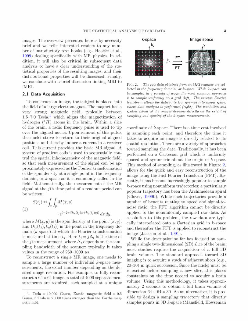
Fig. 2. The raw data obtained from an MRI scanner are col-lected in the frequency domain, or k-space. While k-space canbe sampled in a variety of ways, the most common approachis to sample uniformly on a grid (left). The inverse Fouriertransform allows the data to be transformed into image space,where data analysis is performed (right). The resolution andspatial extent of the images depends directly on the extent ofsampling and spacing of the k-space measurements.

coordinate of k-space. There is a time cost involvedin sampling each point, and therefore the time ittakes to acquire an image is directly related to itsspatial resolution. There are a variety of approachestoward sampling the data. Traditionally, it has beenperformed on a Cartesian grid which is uniformlyspaced and symmetric about the origin of k-space.This method of sampling, as illustrated in Figure 2,allows for the quick and easy reconstruction of theimage using the Fast Fourier Transform (FFT). Re-cently, it has become increasingly popular to samplek-space using nonuniform trajectories; a particularlypopular trajectory has been the Archimedean spiral(Glover, 1999b). While such trajectories provide anumber of benefits relating to speed and signal-to-noise ratio, the FFT algorithm cannot be directlyapplied to the nonuniformly sampled raw data. Asa solution to this problem, the raw data are typi-cally interpolated onto a Cartesian grid in k-spaceand thereafter the FFT is applied to reconstruct theimage (Jackson et al., 1991).

While the description so far has focused on sam-pling a single two-dimensional (2D) slice of the brain,most studies require the acquisition of a full 3Dbrain volume. The standard approach toward 3Dimaging is to acquire a stack of adjacent slices (e.g.,20–30) in quick succession. Since the nuclei must bere-excited before sampling a new slice, this placesconstraints on the time needed to acquire a brainvolume. Using this methodology, it takes approxi-mately 2 seconds to obtain a full brain volume ofdimension 64× 64× 30. As an alternative, it is pos-sible to design a sampling trajectory that directlysamples points in 3D k-space (Mansfield, Howseman

4 M. A. LINDQUIST

and Ordidge, 1989; Mansfield, Coxon and Hykin,1995; Lindquist et al., 2008b). Though this approachwould potentially allow the same number of k-spacepoints to be sampled at a faster rate, the stackedslice approach remains dominant. However, with in-creases in computational power and hardware im-provements, 3D sampling should attract increasedattention.

The process of designing new k-space samplingtrajectories is an interesting mathematical problem,which can easily be generalized to three dimensionsby letting k(t) = (kx(t), ky(t)), kz(t)). The goal is tofind a trajectory k(t) that moves through k-spaceand satisfies the necessary constraints. The trajec-tory is defined as a continuous curve and along thiscurve measurements are made at uniform time inter-vals determined by the sampling bandwidth of thescanner. The trajectory starts at the point (0,0,0)and its subsequent movement is limited byconstraints placed on both its speed and accelera-tion. In addition, there is a finite amount of time thesignal can be measured before the nuclei need to bere-exited and the trajectory is returned to the ori-gin. Finally, the trajectory needs to be space-filling,which implies that each point in the lattice con-tained within some cubic or spherical region aroundthe center of k-space needs to be visited long enoughto make a measurement. The size of this region de-termines the spatial resolution of the subsequent im-age reconstruction. For a more complete formula-tion of the problem, see Lindquist et al. (2008a).The problem bears some resemblance to the trav-eling salesman problem and can be approached inan analogous manner. One application where trajec-tory design is important is rapid imaging (Lindquistet al., 2006, 2008a) and we return to this issue in alater section.

2.2 Statistical Properties of MR Images

As the signal in (1) is measured over two chan-nels, the raw k-space data are complex valued. Itis assumed that both the real and imaginary com-ponent is measured with independent normally dis-tributed error. Since the Fourier transformation isa linear operation, the reconstructed voxel data willalso be complex-valued with both parts followinga normal distribution. In the final stage of the re-construction process, these complex valued measure-ments are separated into magnitude and phase com-ponents. In the vast majority of studies only themagnitude portion of the signal is used in the data

analysis, while the phase portion is discarded. Tra-

ditionally, the phase has not been considered to con-

tain relevant signal information, though models that

use both components (Rowe and Logan, 2004) have

been proposed. It should be noted that the mag-

nitude values no longer follow a normal distribu-

tion, but rather a Rice distribution (Gudbjartsson

and Patz, 1995). The shape of this distribution de-

pends on the signal-to-noise (SNR) ratio within the

voxel. For the special case when no signal is present

(e.g., for voxels outside of the brain), it behaves

like a Rayleigh distribution. When the SNR is high

(e.g., for voxels within the brain) the distribution

is approximately Gaussian. Understanding the dis-

tributional properties of MR images is important,

and this area provides some interesting research op-

portunities for statisticians in terms of developing

methods for estimating the variance of the back-

ground noise and methods for identifying and re-

moving outliers that arise due to acquisition arti-

facts.

2.3 From MRI to fMRI

The data acquisition and reconstruction techniques

outlined in this section provide the means for obtain-

ing a static image of the brain. However, changes

in brain hemodynamics in response to neuronal ac-

tivity impact the local intensity of the MR signal.

Therefore, a sequence of properly acquired brain im-

ages allows one to study changes in brain function

over time.

An fMRI study consists of a series of brain vol-

umes collected in quick succession. The temporal

resolution of the acquired data will depend on the

time between acquisitions of each individual vol-

ume; once the k-space has been sampled, the pro-

cedure is ready to be repeated and a new volume

can be acquired. This is one reason why efficient

sampling of k-space is important. Typically, brain

volumes of dimensions 64×64×30 (i.e. 122,880 vox-

els) are collected at T separate time points through-

out the course of an experiment, where T varies be-

tween 100–2000. Hence, the resulting data consists

of roughly 100,000 time series of length T . On top

of this, the experiment is often repeated for M sub-

jects, where M usually varies between 10 and 40. It

quickly becomes clear that fMRI data analysis is a

time series analysis problem of massive proportions.

THE STATISTICAL ANALYSIS OF fMRI DATA 5

3. UNDERSTANDING fMRI DATA

The ability to connect the measures of brain phys-iology obtained in an fMRI experiment with theunderlying neuronal activity that caused them willgreatly impact the choice of inference procedure andthe subsequent conclusions that can be made. There-fore, it is important to gain some rudimentary un-derstanding of basic brain physiology. The overviewpresented here is brief and interested readers are re-ferred to text books dealing specifically with thesubject (e.g., Huettel, Song and Mccarthy, 2004).In addition, since neuronal activity unfolds both inspace and time, the spatial and temporal resolutionof fMRI studies will limit any conclusions that canbe made from analyzing the data and understand-ing these limitations is paramount. Finally, as rel-atively small changes in brain activity are buriedwithin noisy measurements, it will be important tounderstand the behavior of both the signal and noisepresent in fMRI data and begin discussing how thesecomponents can be appropriately modeled.

3.1 BOLD fMRI

Functional magnetic resonance imaging is mostcommonly performed using blood oxygenation level-dependent (BOLD) contrast (Ogawa et al., 1992) tostudy local changes in deoxyhemoglobin concentra-tion in the brain. BOLD imaging takes advantage ofinherent differences between oxygenated and deoxy-genated hemoglobin. Each of these states has dif-ferent magnetic properties, diamagnetic and para-magnetic respectively, and produces different localmagnetic fields. Due to its paramagnetic proper-ties, deoxy-hemoglobin has the effect of suppressingthe MR signal, while oxy-hemoglobin does not. Thecerebral blood flow refreshes areas of the brain thatare active during the execution of a mental task withoxygenated blood, thereby changing the local mag-netic susceptibility and the measured MR signal inactive brain regions. A series of properly acquiredMR images can therefore be used to study changesin blood oxygenation which, in turn, can be used toinfer brain activity.

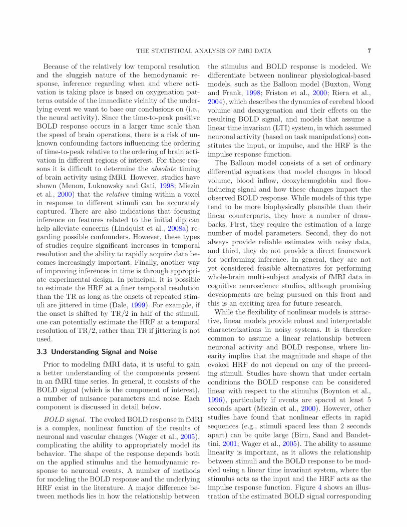
The underlying evoked hemodynamic response toa neural event is typically referred to as the hemo-dynamic response function (HRF). Figure 3A showsthe standard shape used to model the HRF, some-times called the canonical HRF. The increasedmetabolic demands due to neuronal activity leadto an increase in the inflow of oxygenated blood

Fig. 3. (A) The standard canonical model for the HRF usedin fMRI data analysis illustrates the main features of the re-sponse. (B) Examples of empirical HRFs measured over thevisual and motor cortices in response to a visual-motor task.(C) The initial 2 seconds of the empirical HRFs give strongindication of an initial decrease in signal immediately follow-ing activation.

to active regions of the brain. Since more oxygenis supplied than actually consumed, this leads to adecrease in the concentration of deoxy-hemoglobinwhich, in turn, leads to an increase in signal. Thispositive rise in signal has an onset approximately 2seconds after the onset of neural activity and peaks5–8 seconds after that neural activity has peaked(Aguirre, Zarahn and D’Esposito, 1998). After reach-ing its peak level, the BOLD signal decreases to abelow baseline level which is sustained for roughly10 seconds. This effect, known as the post-stimulusundershoot, is due to the fact that blood flow de-creases more rapidly than blood volume, thereby al-lowing for a greater concentration of deoxy-hemoglobinin previously active brain regions.

Several studies have shown evidence of a decreasein oxygenation levels in the time immediately fol-lowing neural activity, giving rise to a decrease inthe BOLD signal in the first 1–2 seconds followingactivation. This decrease is called the initial neg-ative BOLD response or the negative dip (Menonet al., 1995; Malonek and Grinvald, 1996). Figures3B–C illustrate this effect in data collected duringan experiment that stimulated both the visual andmotor cortices. The ratio of the amplitude of the dip

6 M. A. LINDQUIST

compared to the positive BOLD signal depends onthe strength of the magnet and has been reportedto be roughly 20% at 3 Tesla (Yacoub, Le and Hu,1998). There is also evidence that the dip is morelocalized to areas of neural activity (Yacoub, Le andHu, 1998; Duong et al., 2000; Kim, Duong and Kim,2000; Thompson, Peterson and Freeman, 2004) thanthe subsequent rise which appears less spatially spe-cific. Due in part to these reasons, the negative re-sponse has so far not been reliably observed and itsexistence remains controversial (Logothetis, 2000).

3.2 Spatial and Temporal Limitations

There are a number of limitations that restrictwhat fMRI can measure and what can be inferredfrom an fMRI study. Many of these limitations aredirectly linked to the spatial and temporal resolu-tion of the study. When designing an experimentit is therefore important to balance the need foradequate spatial resolution with that of adequatetemporal resolution. The temporal resolution deter-mines our ability to separate brain events in time,while the spatial resolution determines our ability todistinguish changes in an image across spatial loca-tions. The manner in which fMRI data is collectedmakes it impossible to simultaneously increase both,as increases in temporal resolution limit the numberof k-space measurements that can be made in the al-located sampling window and thereby directly influ-ence the spatial resolution of the image. Therefore,there are inherent trade-offs required when deter-mining the appropriate spatial and temporal resolu-tions to use in an fMRI experiment.

One of the benefits of MRI as an imaging tech-nique is its ability to provide detailed anatomicalscans of gray and white matter with a spatial reso-lution well below 1 mm3. However, the time neededto acquire such scans is prohibitively high and cur-rently not feasible for use in functional studies. In-stead, the spatial resolution is typically on the orderof 3 × 3 × 5 mm3, corresponding to image dimen-sions on the order of 64× 64× 30, which can readilybe sampled in approximately 2 seconds. Still, fMRIprovides relatively high spatial resolution comparedwith many other functional imaging techniques. How-ever, it is important to note that the potential highspatial resolution is often limited by a number of fac-tors. First, it is common to spatially smooth fMRIdata prior to analysis which decreases the effectiveresolution of the data. Second, performing popula-tion inference requires the analysis of groups of sub-jects with varying brain sizes and shapes. In order to

compare data across subjects, a normalization pro-cedure is used to warp the brains onto a standardtemplate brain. This procedure introduces spatialimprecision and blurring in the group data. An ob-vious impact of all this blurring is that activation insmall structures may be mislocalized or even missedall together.

Inferences in space can potentially be improvedby advances in data acquisition and preprocessing.The introduction of enhanced spatial inter-subjectnormalization techniques and improved smoothingtechniques would help researchers avoid the mostdramatic effects of blurring the data. Statistical is-sues that arise due to smoothing and normalizationwill be revisited in a later section dealing specificallywith preprocessing. A recent innovation in signal ac-quisition has been the use of multiple coils with dif-ferent spatial sensitivities to simultaneously measurek-space (Sodickson and Manning, 1997; Pruessmannet al., 1999). This approach, known as parallel imag-ing, allows for an increase in the amount of data thatcan be collected in a given time window. Hence, itcan be used to either increase the spatial resolu-tion of an image or decrease the amount of timerequired to sample an image with a certain speci-fied spatial resolution. Parallel imaging techniqueshave already had a great influence on the way datais collected and its role will only increase. The ap-propriate manner to deal with parallel imaging datais a key direction for future research. Designing newways of acquiring and reconstructing multi-coil datais an important area of research where statistics canplay a vital role.

The temporal resolution of an fMRI study de-pends on the time between acquisition of each indi-vidual image, or the repetition time (TR). In mostfMRI studies the TR ranges from 0.5–4.0 seconds.These values indicate a fundamental disconnect be-tween the underlying neuronal activity, which takesplace on the order of tens of milliseconds, and thetemporal resolution of the study. However, the sta-tistical analysis of fMRI data is primarily focused onusing the positive BOLD response to study the un-derlying neural activity. Hence, the limiting factorin determining the appropriate temporal resolutionis generally not considered the speed of data acqui-sition, but rather the speed of the underlying evokedhemodynamic response to a neural event. Since in-ference is based on oxygenation patterns taking place5–8 seconds after activation, TR values in the rangeof 2 seconds are generally deemed adequate.

THE STATISTICAL ANALYSIS OF fMRI DATA 7

Because of the relatively low temporal resolutionand the sluggish nature of the hemodynamic re-sponse, inference regarding when and where acti-vation is taking place is based on oxygenation pat-terns outside of the immediate vicinity of the under-lying event we want to base our conclusions on (i.e.,the neural activity). Since the time-to-peak positiveBOLD response occurs in a larger time scale thanthe speed of brain operations, there is a risk of un-known confounding factors influencing the orderingof time-to-peak relative to the ordering of brain acti-vation in different regions of interest. For these rea-sons it is difficult to determine the absolute timingof brain activity using fMRI. However, studies haveshown (Menon, Luknowsky and Gati, 1998; Miezinet al., 2000) that the relative timing within a voxelin response to different stimuli can be accuratelycaptured. There are also indications that focusinginference on features related to the initial dip canhelp alleviate concerns (Lindquist et al., 2008a) re-garding possible confounders. However, these typesof studies require significant increases in temporalresolution and the ability to rapidly acquire data be-comes increasingly important. Finally, another wayof improving inferences in time is through appropri-ate experimental design. In principal, it is possibleto estimate the HRF at a finer temporal resolutionthan the TR as long as the onsets of repeated stim-uli are jittered in time (Dale, 1999). For example, ifthe onset is shifted by TR/2 in half of the stimuli,one can potentially estimate the HRF at a temporalresolution of TR/2, rather than TR if jittering is notused.

3.3 Understanding Signal and Noise

Prior to modeling fMRI data, it is useful to gaina better understanding of the components presentin an fMRI time series. In general, it consists of theBOLD signal (which is the component of interest),a number of nuisance parameters and noise. Eachcomponent is discussed in detail below.

BOLD signal. The evoked BOLD response in fMRIis a complex, nonlinear function of the results ofneuronal and vascular changes (Wager et al., 2005),complicating the ability to appropriately model itsbehavior. The shape of the response depends bothon the applied stimulus and the hemodynamic re-sponse to neuronal events. A number of methodsfor modeling the BOLD response and the underlyingHRF exist in the literature. A major difference be-tween methods lies in how the relationship between

the stimulus and BOLD response is modeled. Wedifferentiate between nonlinear physiological-basedmodels, such as the Balloon model (Buxton, Wongand Frank, 1998; Friston et al., 2000; Riera et al.,2004), which describes the dynamics of cerebral bloodvolume and deoxygenation and their effects on theresulting BOLD signal, and models that assume alinear time invariant (LTI) system, in which assumedneuronal activity (based on task manipulations) con-stitutes the input, or impulse, and the HRF is theimpulse response function.

The Balloon model consists of a set of ordinarydifferential equations that model changes in bloodvolume, blood inflow, deoxyhemoglobin and flow-inducing signal and how these changes impact theobserved BOLD response. While models of this typetend to be more biophysically plausible than theirlinear counterparts, they have a number of draw-backs. First, they require the estimation of a largenumber of model parameters. Second, they do notalways provide reliable estimates with noisy data,and third, they do not provide a direct frameworkfor performing inference. In general, they are notyet considered feasible alternatives for performingwhole-brain multi-subject analysis of fMRI data incognitive neuroscience studies, although promisingdevelopments are being pursued on this front andthis is an exciting area for future research.

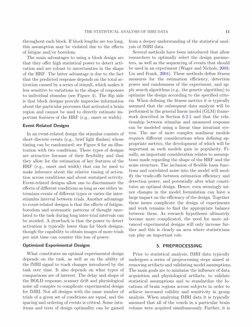
While the flexibility of nonlinear models is attrac-tive, linear models provide robust and interpretablecharacterizations in noisy systems. It is thereforecommon to assume a linear relationship betweenneuronal activity and BOLD response, where lin-earity implies that the magnitude and shape of theevoked HRF do not depend on any of the preced-ing stimuli. Studies have shown that under certainconditions the BOLD response can be consideredlinear with respect to the stimulus (Boynton et al.,1996), particularly if events are spaced at least 5seconds apart (Miezin et al., 2000). However, otherstudies have found that nonlinear effects in rapidsequences (e.g., stimuli spaced less than 2 secondsapart) can be quite large (Birn, Saad and Bandet-tini, 2001; Wager et al., 2005). The ability to assumelinearity is important, as it allows the relationshipbetween stimuli and the BOLD response to be mod-eled using a linear time invariant system, where thestimulus acts as the input and the HRF acts as theimpulse response function. Figure 4 shows an illus-tration of the estimated BOLD signal corresponding

8 M. A. LINDQUIST

to two different types of stimulus patterns. In a lin-ear system framework the signal at time t, x(t), ismodeled as the convolution of a stimulus functionv(t) and the hemodynamic response h(t), that is,

x(t) = (v ∗ h)(t).(2)

Here h(t) is either assumed to take a canonical form,or alternatively modeled using a set of linear basisfunctions.

Another important modeling aspect is that thetiming and shape of the HRF are known to varyacross the brain, within an individual and acrossindividuals (Aguirre, Zarahn and D’Esposito, 1998;Schacter et al., 1997). Part of the variability is dueto the underlying configuration of the vascular bed,which may cause differences in the HRF across brainregions in the same task for purely physiological rea-sons (Vazquez et al., 2006). Another source of vari-ability is differences in the pattern of evoked neuralactivity in regions performing different functions re-lated to the same task. It is important that theseregional variations are accounted for when model-ing the BOLD signal and we return to this issue ina later section.

In general, one of the major shortfalls when an-alyzing fMRI data is that users typically assume acanonical HRF (Grinband et al., 2008), which leavesopen the possibility for mismodeling the signal inlarge portions of the brain (Loh, Lindquist and Wa-ger, 2008). There has therefore been a movementtoward both using more sophisticated models andenhanced model diagnostics. Both of these areas fall

squarely in the purview of statisticians, and promiseto have increased importance in the future.

Noise and nuisance signal. The measured fMRIsignal is corrupted by random noise and various nui-sance components that arise due both to hardwarereasons and the subjects themselves. For instance,fluctuations in the MR signal intensity caused bythermal motion of electrons within the subject andthe scanner gives rise to noise that tends to be highlyrandom and independent of the experimental task.The amount of thermal noise increases linearly asa function of the field strength of the scanner, withhigher field strengths giving rise to more noise. How-ever, it does not exhibit spatial structure and its ef-fects can be minimized by averaging the signal overmultiple data points. Another source of variability inthe signal is due to scanner drift, caused by scannerinstabilities, which result in slow changes in voxel in-tensity over time (low-frequency noise). The amountof drift varies across space, and it is important toinclude this source of variation in your models. Fi-nally, physiological noise due to patient motion, res-piration and heartbeat cause fluctuations in signalacross both space and time. Physiological noise canoften be modeled and the worst of its effects re-moved. In the next section we discuss how to correctfor subject motion as part of the preprocessing stepof the analysis. However, heart-rate and respirationgives rise to periodic fluctuations that are difficult tomodel. According to the Nyquist criteria, it is nec-essary to have a sampling rate at least twice as highas the frequency of the periodic function one seeks

Fig. 4. The BOLD response is typically modeled as the convolution of the stimulus function with the HRF. Varying stimuluspatterns will give rise to responses with radically different features.

THE STATISTICAL ANALYSIS OF fMRI DATA 9

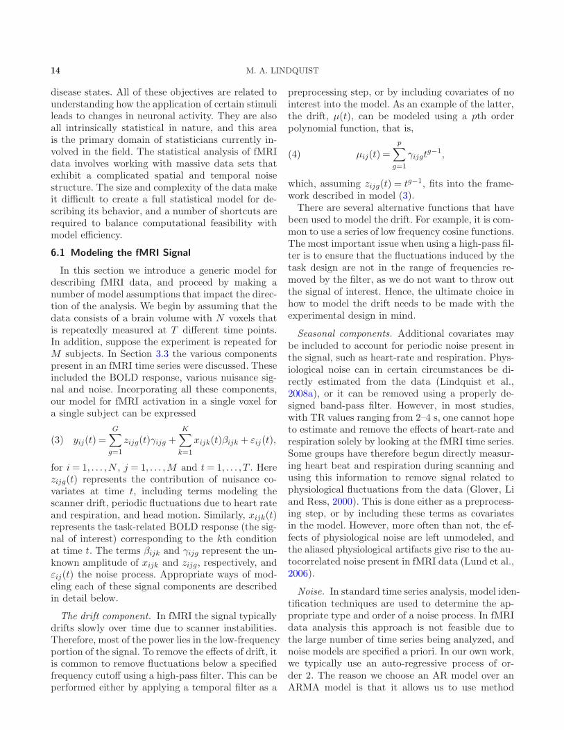
to model. If the TR is too low, which is true in mostfMRI studies, there will be problems with aliasing;see Figure 5A for an illustration. In this situation theperiodic fluctuations will be distributed throughoutthe time course giving rise to temporal autocorrela-tion. Noise in fMRI is typically modeled using eitheran AR(p) or an ARMA(1,1) process (Purdon et al.,2001), where the autocorrelation is thought to bedue to an unmodeled nuisance signal. If these termsare properly removed, there is evidence that the re-sulting error term corresponds to white noise (Lundet al., 2006). Note that for high temporal resolutionstudies, heart-rate and respiration can be estimatedand included in the model, or alternatively removedthrough application of a band-pass filter.

The spatiotemporal behavior of the noise processis complex. Figure 5B shows a time course froma single voxel sampled at high temporal resolution(60 ms), as well as its power spectrum. The powerspectrum indicates periodic oscillations in the sig-nal due to physiological effects and a low-frequencycomponent corresponding to signal drift. At this res-olution it is relatively straightforward to remove theeffects of these nuisance functions by applying anappropriate filter. In contrast, Figure 5C shows atime course sampled at a more standard resolution(1 s). At this resolution, the sampling rate is toolow to effectively model physiological noise and itgives rise to temporal autocorrelation clearly visiblein the accompanying autocorrelation plot. Finally,Figure 5D shows spatial maps of the model parame-ters from an AR(2) model estimated for each voxel’snoise data. It is clear that the behavior of the noiseis not consistent throughout the image, indicatingspatial dependence. In fact, it is clearly possible tomake out rough anatomical detail in the maps, indi-cating higher amounts of variability in certain brainregions.

4. EXPERIMENTAL DESIGN

The experimental design of an fMRI study is com-plicated, as it not only involves the standard issuesrelevant to psychological experiments, but also is-sues related to data acquisition and stimulus pre-sentation. Not all designs with the same number oftrials of a given set of conditions are equal, and thespacing and ordering of events is critical. What con-stitutes an optimal experimental design depends onthe psychological nature of the task, the ability ofthe fMRI signal to track changes introduced by the

task over time and the specific comparisons that oneis interested in making. In addition, as the efficiencyof the subsequent statistical analysis is directly re-lated to the experimental design, it is important thatit be carefully considered during the design process.

A good experimental design attempts to maxi-mize both statistical power and psychological valid-ity. The statistical performance can be characterizedby its estimation efficiency (i.e., the ability to esti-mate the HRF) and its detection power (i.e., theability to detect significant activation). The psycho-logical validity is often measured by the random-ness of the stimulus presentation, as this helps con-trol for issues related to anticipation, habituationand boredom. When designing an experiment thereis inherent trade-offs between estimation efficiency,detection power and randomness. The optimal bal-ance between the three ultimately depends on thegoals of the experiment and the combination of con-ditions one is interested in studying. For example,a design used to localize areas of brain activationstresses high detection power at the expensive of es-timation efficiency and randomness.

While the area of experimental design is a natu-ral domain for statisticians to conduct research, ithas so far been largely unexplored by members ofthe field. Currently there are two major classes offMRI experimental designs: block designs and event-related designs. In the following sections we describeeach type and discuss the applications for whichthey are best suited. In addition, we also discussways of optimizing the experimental design.

Block Designs

In a block design the different experimental condi-tions are separated into extended time intervals, orblocks. For example, one might repeat the processof interest (e.g., finger tapping) during an experi-mental block (A) and have the subject rest duringa control block (B); see Figure 6. The A–B com-parison can than be used to compare differences insignal between the conditions. In general, increas-ing the length of each block will lead to a largerevoked response during the task. This increases theseparation in signal between blocks, which, in turn,leads to higher detection power. However, in con-trast, it is also important to include multiple transi-tions between conditions, as otherwise differences insignal due to low-frequency drift may be confused fordifferences in task conditions. In addition, it is im-portant that the same mental processes are evoked

10 M. A. LINDQUIST

Fig. 5. (A) The Nyquist criteria states that it is necessary to sample at a frequency at least twice as high as the frequencyof the periodic function one seeks to model to avoid aliasing. As an illustration assume that the signal is measured at the timepoints indicated by circles. In this situation it is impossible to determine which of the two periodic signals shown in the plotgive rise to the observed measurements. (B) An fMRI time course measured at a single voxel sampled with 60 ms resolution. Itspower spectrum indicates components present in the signal whose periodicity corresponds to low-frequency drift and physiologicaleffects. (C) An fMRI time course measured with 1 s resolution. The autocorrelation function indicates autocorrelation presentin the signal. (D) Spatial maps of the model parameters from an AR(2) model (i.e. φ1, φ2 and σ), estimated from each voxel’snoise data, indicates clear spatial dependence.

Fig. 6. The two most common classes of experimental design are block designs and event-related designs. In a block design(top) experimental conditions are separated into extended time intervals, or blocks, of the same type. In an event-related design(bottom) the stimulus consists of short discrete events whose timing and order can be randomized.

THE STATISTICAL ANALYSIS OF fMRI DATA 11

throughout each block. If block lengths are too long,this assumption may be violated due to the effectsof fatigue and/or boredom.

The main advantages to using a block design arethat they offer high statistical power to detect acti-vation and are robust to uncertainties in the shapeof the HRF. The latter advantage is due to the factthat the predicted response depends on the total ac-tivation caused by a series of stimuli, which makes itless sensitive to variations in the shape of responsesto individual stimulus (see Figure 4). The flip sideis that block designs provide imprecise informationabout the particular processes that activated a brainregion and cannot be used to directly estimate im-portant features of the HRF (e.g., onset or width).

Event-Related Designs

In an event-related design the stimulus consists ofshort discrete events (e.g., brief light flashes) whosetiming can be randomized; see Figure 6 for an illus-tration with two conditions. These types of designsare attractive because of their flexibility and thatthey allow for the estimation of key features of theHRF (e.g., onset and width) that can be used tomake inference about the relative timing of activa-tion across conditions and about sustained activity.Event-related designs allow one to discriminate theeffects of different conditions as long as one either in-termixes events of different types or varies the inter-stimulus interval between trials. Another advantageto event-related designs is that the effects of fatigue,boredom and systematic patterns of thought unre-lated to the task during long inter-trial intervals canbe avoided. A drawback is that the power to detectactivation is typically lower than for block designs,though the capability to obtain images of more trialsper unit time can counter this loss of power.

Optimized Experimental Designs

What constitutes an optimal experimental designdepends on the task, as well as on the ability ofthe fMRI signal to track changes introduced by thetask over time. It also depends on what types ofcomparisons are of interest. The delay and shape ofthe BOLD response, scanner drift and physiologicalnoise all conspire to complicate experimental designfor fMRI. Not all designs with the same number oftrials of a given set of conditions are equal, and thespacing and ordering of events is critical. Some intu-itions and tests of design optimality can be gained

from a deeper understanding of the statistical anal-ysis of fMRI data.

Several methods have been introduced that allowresearchers to optimally select the design parame-ters, as well as the sequencing of events that shouldbe used in an experiment (Wager and Nichols, 2003;Liu and Frank, 2004). These methods define fitnessmeasures for the estimation efficiency, detectionpower and randomness of the experiment, and ap-ply search algorithms (e.g., the genetic algorithm) tooptimize the design according to the specified crite-ria. When defining the fitness metrics it is typicallyassumed that the subsequent data analysis will beperformed in the general linear model (GLM) frame-work described in Section 6.2.1 and that the rela-tionship between stimulus and measured responsecan be modeled using a linear time invariant sys-tem. The use of more complex nonlinear modelsrequires different considerations when defining ap-propriate metrics, the development of which will beimportant as such models gain in popularity. Fi-nally, an important consideration relates to assump-tions made regarding the shape of the HRF and thenoise structure. The inclusion of flexible basis func-tions and correlated noise into the model will mod-ify the trade-offs between estimation efficiency anddetection power, and potentially alter what consti-tutes an optimal design. Hence, even seemingly mi-nor changes in the model formulation can have alarge impact on the efficiency of the design. Togetherthese issues complicate the design of experimentsand work remains to find the appropriate balancebetween them. As research hypotheses ultimatelybecome more complicated, the need for more ad-vanced experimental designs will only increase fur-ther and this is clearly an area where statisticianscan play an important role.

5. PREPROCESSING

Prior to statistical analysis, fMRI data typicallyundergoes a series of preprocessing steps aimed atremoving artifacts and validating model assumptions.The main goals are to minimize the influence of dataacquisition and physiological artifacts, to validatestatistical assumptions and to standardize the lo-cations of brain regions across subjects in order toachieve increased validity and sensitivity in groupanalysis. When analyzing fMRI data it is typicallyassumed that all of the voxels in a particular brainvolume were acquired simultaneously. Further, it is

12 M. A. LINDQUIST

assumed that each data point in a specific voxel’stime series only consists of a signal from that voxel(i.e., that the participant did not move in betweenmeasurements). Finally, when performing group anal-ysis and making population inference, all individualbrains are assumed to be registered, so that eachvoxel is located in the same anatomical region forall subjects. Without preprocessing the data priorto analysis, none of these assumptions would holdand the resulting statistical analysis would be in-valid.

The major steps involved in fMRI preprocessingare slice timing correction, realignment, coregistra-tion of structural and functional images, normaliza-tion and smoothing. Below each step is discussed indetail.

Slice Timing Correction

When analyzing 3D fMRI data it is typically as-sumed that the whole brain is measured simulta-neously. In reality, because the brain volume con-sists of multiple slices that are sampled sequentially,

Fig. 7. (A) Illustration of slice timing correction. Assumethree brain slices, exhibiting a similar time course, are sam-pled sequentially during each TR (top row). Since the voxelsare sampled at different time points relative to one another,their respective time courses will appear shifted (bottom row).Slice timing correction shifts the time series so they can beconsidered to have been measured simultaneously. (B) Illustra-tion of normalization using warping. A high resolution image(left) is warped onto a template image (center), resulting in anormalized image (right).

and therefore at different time points, similar timecourses from different slices will be temporally shiftedrelative to one another. Figure 7A illustrates thepoint. Assume that three voxels contained in threeadjacent slices exhibit the same true underlying tem-poral profile. Due to the fact that they are sam-pled at different time points relative to one another,the corresponding measured time courses will ap-pear different. Slice timing correction involves shift-ing each voxel’s time course so that one can as-sume they were measured simultaneously. This canbe done either using interpolation or the Fouriershift theorem to correct for differences in acquisi-tion times.

Motion Correction

An important issue involved in any fMRI study isthe proper handling of any subject movement thatmay have taken place during data acquisition. Evensmall amounts of head motion during the course ofan experiment can be a major source of error if nottreated correctly. When movement occurs, the sig-nal from a specific voxel will be contaminated bythe signal from neighboring voxels and the result-ing data can be rendered useless. Therefore, it is ofgreat importance to accurately estimate the amountof motion and to use this information to correctthe images. If the amount of motion is deemed toosevere, it may result in the subject being removedcompletely from the study.

The first step in correcting for motion is to findthe best possible alignment between the input im-age and some target image (e.g., the first image orthe mean image). A rigid body transformation in-volving 6 variable parameters is used. This allowsthe input image to be translated (shifted in the x,y and z directions) and rotated (altered roll, pitchand yaw) to match the target image. Usually, thematching process is performed by minimizing somecost function (e.g., sums of squared differences) thatassesses similarity between the two images. Once theparameters that achieve optimal realignment are de-termined, the image is resampled using interpolationto create new motion corrected voxel values. Thisprocedure is repeated for each individual brain vol-ume.

Coregistration and Normalization

Functional MRI data is typically of low spatialresolution and provides relatively little anatomicaldetail. Therefore, it is common to map the results

THE STATISTICAL ANALYSIS OF fMRI DATA 13

obtained from functional data onto a high resolutionstructural MR image for presentation purposes. Theprocess of aligning structural and functional images,called coregistration, is typically performed using ei-ther a rigid body (6 parameters) or an affine (12parameters) transformation.

For group analysis, it is important that each voxellie within the same brain structure for each individ-ual subject. Of course individual brains have differ-ent shapes and features, but there are regularitiesshared by every nonpathological brain. Normaliza-tion attempts to register each subjects anatomy toa standardized stereotaxic space defined by a tem-plate brain [e.g., the Talairach or Montreal Neuro-logical Institute (MNI) brain]. In this scenario usinga rigid body transformation is inappropriate due tothe inherent differences in the subjects brains. In-stead, it is common to use nonlinear transformationsto match local features. One begins by estimating asmooth continuous mapping between the points inan input image with those in the target image. Next,the mapping is used to resample the input image sothat it is warped onto the target image. Figure 7B il-lustrates the process, where a high resolution imageis warped onto a template image, resulting in a nor-malized image that can be compared with similarlynormalized images obtained from other subjects.

The main benefits of normalizing data are thatspatial locations can be reported and interpretedin a consistent manner, results can be generalizedto a larger population and results can be comparedacross studies and subjects. The drawbacks are thatit reduces spatial resolution and may introduce er-rors due to interpolation.

Spatial Smoothing

It is common practice to spatially smooth fMRIdata prior to analysis. Smoothing typically involvesconvolving the functional images with a Gaussiankernel, often described by the full width of the ker-nel at half its maximum height (FWHM). Commonvalues for the kernel widths vary between 4–12 mmFWHM. There are several reasons why it is com-mon to smooth fMRI data. First, it may improveinter-subject registration and overcome limitationsin the spatial normalization by blurring any resid-ual anatomical differences. Second, it ensures thatthe assumptions of random field theory (RFT), com-monly used to correct for multiple-comparisons, arevalid. A rough estimate of the amount of smooth-ing required to meet the assumptions of RFT is a

FWHM of 3 times the voxel size (e.g., 9 mm for3 mm voxels). Third, if the spatial extent of a re-gion of interest is larger than the spatial resolution,smoothing may reduce random noise in individualvoxels and increase the signal-to-noise ratio withinthe region.

The process of spatially smoothing an image isequivalent to applying a low-pass filter to the sam-pled k-space data prior to reconstruction. This im-plies that much of the acquired data is discarded asa byproduct of smoothing and temporal resolutionis sacrificed without gaining any benefits. Addition-ally, acquiring an image with high spatial resolutionand thereafter smoothing the image does not lead tothe same results as directly acquiring a low resolu-tion image. The signal-to-noise ratio during acquisi-tion increases as the square of the voxel volume, soacquiring small voxels means that signal is lost thatcan never be recovered. Hence, it is optimal in termsof sensitivity to acquire images at the desired resolu-tion and not employ smoothing. Some recent acqui-sition schemes have been designed to acquire imagesat the final functional resolution desired (Lindquistet al., 2008b). This allows for much more rapid im-age acquisition, as time is not spent acquiring in-formation that will be discarded in the subsequentanalysis.

While all the preprocessing steps outlined aboveare essential for the standard model assumptions re-quired for statistical analysis to hold, there needs tobe a clear understanding of the effects they have onboth the spatial and temporal correlation structure.More generally, it is necessary to study the interac-tions among the individual preprocessing steps. Forexample, is it better to perform slice timing correc-tion or realignment first, and how will this choiceimpact the resulting data? Ideally there would beone model for both, that also performs outlier de-tection and correction for physiological noise. Therehas been increased interest in developing generativemodels that incorporate multiple steps at once, andthis is another problem with a clear statistical com-ponent that promises to play an important role inthe future.

6. DATA ANALYSIS

There are several common objectives in the anal-ysis of fMRI data. These include localizing regionsof the brain activated by a certain task, determiningdistributed networks that correspond to brain func-tion and making predictions about psychological or

14 M. A. LINDQUIST

disease states. All of these objectives are related tounderstanding how the application of certain stimulileads to changes in neuronal activity. They are alsoall intrinsically statistical in nature, and this areais the primary domain of statisticians currently in-volved in the field. The statistical analysis of fMRIdata involves working with massive data sets thatexhibit a complicated spatial and temporal noisestructure. The size and complexity of the data makeit difficult to create a full statistical model for de-scribing its behavior, and a number of shortcuts arerequired to balance computational feasibility withmodel efficiency.

6.1 Modeling the fMRI Signal

In this section we introduce a generic model fordescribing fMRI data, and proceed by making anumber of model assumptions that impact the direc-tion of the analysis. We begin by assuming that thedata consists of a brain volume with N voxels thatis repeatedly measured at T different time points.In addition, suppose the experiment is repeated forM subjects. In Section 3.3 the various componentspresent in an fMRI time series were discussed. Theseincluded the BOLD response, various nuisance sig-nal and noise. Incorporating all these components,our model for fMRI activation in a single voxel fora single subject can be expressed

yij(t) =G∑

g=1

zijg(t)γijg +K∑

k=1

xijk(t)βijk + εij(t),(3)

for i = 1, . . . ,N , j = 1, . . . ,M and t = 1, . . . , T . Herezijg(t) represents the contribution of nuisance co-variates at time t, including terms modeling thescanner drift, periodic fluctuations due to heart rateand respiration, and head motion. Similarly, xijk(t)represents the task-related BOLD response (the sig-nal of interest) corresponding to the kth conditionat time t. The terms βijk and γijg represent the un-known amplitude of xijk and zijg, respectively, andεij(t) the noise process. Appropriate ways of mod-eling each of these signal components are describedin detail below.

The drift component. In fMRI the signal typicallydrifts slowly over time due to scanner instabilities.Therefore, most of the power lies in the low-frequencyportion of the signal. To remove the effects of drift, itis common to remove fluctuations below a specifiedfrequency cutoff using a high-pass filter. This can beperformed either by applying a temporal filter as a

preprocessing step, or by including covariates of nointerest into the model. As an example of the latter,the drift, µ(t), can be modeled using a pth orderpolynomial function, that is,

µij(t) =p∑

g=1

γijgtg−1,(4)

which, assuming zijg(t) = tg−1, fits into the frame-work described in model (3).

There are several alternative functions that havebeen used to model the drift. For example, it is com-mon to use a series of low frequency cosine functions.The most important issue when using a high-pass fil-ter is to ensure that the fluctuations induced by thetask design are not in the range of frequencies re-moved by the filter, as we do not want to throw outthe signal of interest. Hence, the ultimate choice inhow to model the drift needs to be made with theexperimental design in mind.

Seasonal components. Additional covariates maybe included to account for periodic noise present inthe signal, such as heart-rate and respiration. Phys-iological noise can in certain circumstances be di-rectly estimated from the data (Lindquist et al.,2008a), or it can be removed using a properly de-signed band-pass filter. However, in most studies,with TR values ranging from 2–4 s, one cannot hopeto estimate and remove the effects of heart-rate andrespiration solely by looking at the fMRI time series.Some groups have therefore begun directly measur-ing heart beat and respiration during scanning andusing this information to remove signal related tophysiological fluctuations from the data (Glover, Liand Ress, 2000). This is done either as a preprocess-ing step, or by including these terms as covariatesin the model. However, more often than not, the ef-fects of physiological noise are left unmodeled, andthe aliased physiological artifacts give rise to the au-tocorrelated noise present in fMRI data (Lund et al.,2006).

Noise. In standard time series analysis, model iden-tification techniques are used to determine the ap-propriate type and order of a noise process. In fMRIdata analysis this approach is not feasible due tothe large number of time series being analyzed, andnoise models are specified a priori. In our own work,we typically use an auto-regressive process of or-der 2. The reason we choose an AR model over anARMA model is that it allows us to use method

THE STATISTICAL ANALYSIS OF fMRI DATA 15

of moments rather than maximum likelihood pro-cedures to estimate the noise parameters. This sig-nificantly speeds-up computation time when repeat-edly fitting the model to tens of thousands of timeseries. Choosing the order of the AR process to be2 has been empirically determined to provide themost parsimonious model that is able to account forautocorrelation present in the signal due to aliasedphysiological artifacts.

The BOLD response. The relationship betweenstimuli and BOLD response is typically modeled us-ing a linear time invariant (LTI) system, where thestimulus acts as the input and the HRF acts as theimpulse response function. See Figure 4 for an illus-tration of how the BOLD response varies depend-ing on the stimuli. A linear time invariant systemis characterized by the following properties: scaling,superposition and time-invariance. Scaling impliesthat if the input is scaled by a factor b, then theBOLD response will be scaled by the same factor.This is important as it implies that the amplitude ofthe measured signal provides a measure of the am-plitude of neuronal activity. Therefore, the relativedifference in amplitude between two conditions canbe used to infer that the neuronal activity was sim-ilarly different. Superposition implies that the re-sponse to two different stimuli applied together isequal to the sum of the individual responses. Finally,time-invariance implies that if a stimulus is shiftedby a time t, then the response is also shifted by t.These three properties allow us to differentiate be-tween responses in various brain regions to multipleclosely spaced stimuli.

In our model we allow for K different conditions tobe applied throughout the course of the experiment(e.g., varying degrees of painful stimuli). The BOLDresponse portion of the model can thus be written

sij(t) =K∑

k=1

βijk

∫hij(u)vk(t− u)du,(5)

where hij(t) is the HRF, vk(t) the stimulus func-tion and βijk the signal amplitude for condition k

at voxel i in the jth subject.

Model summary. For most standard fMRI exper-iments we can summarize model (3) as

yij(t) =p∑

g=1

γijgtg−1

+K∑

k=1

βijk

∫hij(u)vk(t− u)du(6)

+ εij(t),

where εij is assumed to follow an AR(2) process. Inmatrix form this can be written

yij = Zijγij + Xijβij + εij,(7)

where γij = (γij1, . . . , γijp)T , βij = (βij1, . . . ,

βijK)T , Zij is a T × p matrix with columns corre-sponding to the polynomial functions, and Xij is aT × K matrix with columns corresponding to thepredicted BOLD response for each condition.

Further, the model in (7) can be combined acrossvoxels as follows:

Yj = XjBj + ZjGj + Ej.(8)

Here Yj is a T × N matrix, where each column isa time series corresponding to a single brain voxeland each row is the collection of voxels that makeup an image at a specific time point. The matricesXj and Zj are the common design matrices usedfor each voxel. Finally, Bj = (β1j , . . . ,βNj), Gj =(γ1j, . . . ,γNj) and Ej = (ε1j , . . . ,εNj). The vector-ized variance of E is typically assumed to be sepa-rable in time and space. In addition, somewhat sur-prisingly, the spatial covariance is often assumed tobe negligible compared to the temporal covarianceand therefore ignored.

While (8) provides a framework for a full spatio-temporal model of brain activity, it is currently notconsidered a feasible alternative due to the extremecomputational demands required for model fitting.Instead, model (7) is applied to each voxel sepa-rately, and spatial concerns are incorporated at alater stage (see below). Alternatively, the matrix Yj

is sometimes analyzed using Multivariate methodsas described in Section 6.3.

6.2 Localizing Brain Activity

The assumptions that one makes regarding theBOLD response fundamentally impact the analysiswhen using model (7). In most controlled experi-ments it is reasonable to assume that the stimulusfunction vk(t) is known and equivalent to the exper-imental paradigm (e.g., a vector of zeros and oneswhere 1 represents time points when the stimulusis “on” and 0 when it is “off”). If one further as-sumes that the HRF is known a priori, (7) revertsto a multiple regression model with known signal

16 M. A. LINDQUIST

components and unknown amplitudes. These are theassumptions made in the hugely popular GLM ap-proach (Worsley and Friston, 1995; Friston et al.,2002), though the assumption regarding fixed HRFcan be relaxed. However, in many areas of psycho-logical inquiry (e.g., emotion and stress), it may bedifficult to specify information regarding the stimu-lus function a priori. If one is unwilling to make anyassumptions regarding the exact timing of neuronalactivity, alternative methods may be more appropri-ate for analyzing the data. In the next two sectionsboth scenarios will be discussed.

6.2.1 The general linear model approach. The gen-eral linear model (GLM) approach has arguably be-come the dominant way to analyze fMRI data. Itmodels the time series as a linear combination of sev-eral different signal components and tests whetheractivity in a brain region is systematically relatedto any of these known input functions. The simplestversion of the GLM assumes that both the stimu-lus function and the HRF are known. The stimu-lus is assumed to be equivalent to the experimentalparadigm, while the HRF is modeled using a canon-ical HRF, typically either a gamma function or thedifference between two gamma functions (see Fig-ure 5). Under these assumptions, the convolutionterm in the BOLD response is a known function and(7) reverts to a standard multiple linear regressionmodel. The BOLD response can be summarized in adesign matrix X, containing a separate column foreach of the K predictors; see Figure 8 for an examplewhen K = 2.

In the remainder of the section we will, for simplic-ity, assume that the nuisance term Z is accounted forand can be ignored. Further, we assume a separate,but identical, model for each voxel and suppress thevoxel index. Hence, the data for subject j at voxel ican be written

yj = Xjβj + εj,(9)

where εj ∼ N(0,V) with the structure of the covari-ance matrix V corresponding to an AR(2) processwith unknown parameters φ1, φ2 and σ. The modelparameters can be estimated using a Cochrane–Orcutt fitting procedure, where the variance compo-nents are estimated using the Yule–Walker method(Brockwell and Davis, 1998). After fitting the model,one can test for an effect cT βj where c is a contrastvector. The contrast vector can be used to estimatesignal magnitudes in response to a single condition,an average over multiple conditions or the differencein magnitude between two conditions. Hypothesistesting is performed in the usual manner by testingindividual model parameters using a t-test and sub-sets of parameters using a partial F -test. Since thecovariance matrix has to be estimated, a Satterth-waite approximation is used to calculate the effec-tive degrees of freedom for the test statistics. Thisprocedure is repeated for brain voxel and the resultsare summarized in a statistical map consisting of animage whose voxel measurements correspond to thetest statistic calculated at that particular voxel.

While the GLM is a simple and powerful approachtoward modeling the data, it is also extremely rigid.Even minor mismodeling (e.g., incorrect stimulusfunction or HRF) can result in severe power loss,and can inflate the false positive rate beyond thenominal value. Due to the massive amount of data,examining the appropriateness of the model is chal-lenging and standard methods of model diagnosticsare not feasible. Recently some techniques have beenintroduced (Luo and Nichols, 2003; Loh, Lindquistand Wager, 2008) that allow one to quickly deter-mine, through graphical representations, areas inthe brain where assumptions are violated and modelmisfit may be present. However, in the vast major-ity of studies no model checking is performed, call-ing into question the validity of the results. Movingtoward using more sophisticated models, as well as

Fig. 8. In an fMRI experiment with two conditions (A and B), the stimulus function is convolved with a canonical HRFto obtain two sets of predicted BOLD responses. The responses are placed into the columns of a design matrix X and used tocompute whether there is significant signal corresponding to the two conditions in a particular time course.

THE STATISTICAL ANALYSIS OF fMRI DATA 17

increased use of diagnostics, is an important area ofcurrent and future research. In both of these areasstatisticians can play an important role.

As mentioned in Section 3.3, the shape of the HRFmay vary across both space and subjects. Therefore,assuming that the shape of the HRF is constantacross all voxels and subjects may give rise to sig-nificant mismodeling in large parts of the brain. Wecan relax this assumption by expressing the HRF asa linear combination of reference waveforms. Thiscan be done in the GLM framework by convolvingthe same stimulus function with multiple canonicalwaveforms and entering them into multiple columnsof X for each condition. These reference waveformsare called basis functions, and the predictors for anevent type constructed using different basis func-tions can combine linearly to better fit the evokedBOLD responses. The ability of a basis set to cap-ture variations in hemodynamic responses dependsboth on the number and shape of the reference wave-forms. There is a fundamental tradeoff between flex-ibility to model variations and power, as flexiblemodels can model noise and produce noisier parame-ter estimates. In addition, the inclusion of additionalmodel parameters decreases the number of degreesof freedom for the subsequent test statistic.

One of the most flexible models, a finite impulseresponse (FIR) basis set, contains one free parame-ter for every time-point following stimulation in ev-ery cognitive event-type that is modeled (Glover,1999a; Goutte, Nielsen and Hansen, 2000). Thus,the model is able to estimate an HRF of arbitraryshape for each event type in every voxel of the brain.Another possible choice is to use the canonical HRFtogether with its temporal derivative in order to al-low for small shifts in the onset of the HRF. Otherchoices of basis sets include those composed of prin-cipal components (Aguirre, Zarahn and D’Esposito,1998; Woolrich, Behrens and Smith, 2004), cosinefunctions (Zarahn, 2002), radial basis functions (Ri-era et al., 2004), spectral basis sets (Liao et al.,2002) and inverse logit functions (Lindquist and Wa-ger, 2007b). For a critical evaluation of various basissets, see Lindquist and Wager (2007b) and Lindquistet al. (2008c).

Multi-subject analysis. The analysis so far has beenconcerned with single subject data. However, re-searchers typically want to make conclusions on pop-ulation effects, and statistical analysis needs to beextended to incorporate information from a groupof subjects. Multi-subject fMRI data is intrinsically

hierarchical in nature, with lower-level observations(e.g., individual subjects) nested within higher levels(e.g., groups of subjects). Multi-level models providea framework for performing mixed-effects analysison multi-subject fMRI data. In fMRI it is commonto use a two-level model where the first level dealswith individual subjects and the second level dealswith groups of subjects. In the first-level the dataare autocorrelated with a relatively large number ofobservations, while in the second-level we have IIDdata with relatively few observations. The first-levelmodel can be written

y = Xβ + ε,(10)

where y = (yT1 , . . . ,yT

M )T , X = diag(X1, . . . ,XM ),β = (βT

1 , . . . ,βTM )T , ε = (εT

1 , . . . ,εTM )T and Var(ε) =

V where V = diag(VT1 , . . . ,VT

M).The second-level model can be written

β = XGβG + εG,(11)

where εG ∼ N(0, Iσ2G). Here XG is the second-level

design matrix (e.g., separating cases from controls)and βG the vector of second-level parameters. Thetwo-level model can be combined into a single levelmodel, which can be expressed as

y = XXGβG + XεG + ε.(12)

Estimation of the regression parameters and vari-ance components can be performed iteratively, withregression parameters estimated using GLS and vari-ance components estimated using restricted maxi-mum likelihood (ReML) and the EM-algorithm.

Recently, these types of multi-level mixed-effectsmodels have become popular in the neuroimagingcommunity due to their ability to perform valid pop-ulation level inference (e.g., Friston et al., 2002; Beck-mann, Jenkinson and Smith, 2003). However, be-cause of the massive amount of data being analyzedand the fact that it must be feasible to repeatedlyfit the model across all brain voxels, the most com-monly used techniques are by necessity simplistic.For example, they do not readily allow for unbal-anced designs and missing data. However, both is-sues are prevalent in fMRI data analysis. Missingdata may be present in a study because of artifactsand errors due to the complexity of data acquisi-tion (including human error), while unbalanced de-signs are important because of interest in relatingbrain activity to performance and other variablesthat cannot be experimentally controlled. The in-troduction of techniques for performing rapid esti-mation of multi-level model parameters that allow

18 M. A. LINDQUIST

for this type of data is of utmost importance. Multi-level models have been heavily researched in the sta-tistical community, and statisticians can play an im-portant role in developing methods tailored directlyto the complexities of fMRI data analysis.

Spatial modeling. Up to this point the entire anal-ysis procedure outlined in this section has been uni-variate, that is, performed separately at each voxel.Indeed, one of the most common short cuts used inthe field is, somewhat surprisingly, to perform fMRIdata analysis in a univariate setting (the so-called“massive univariate approach”), where each voxelis modeled and processed independently of the oth-ers. At the model-level this approach assumes thatneighboring voxels are independent, which is gen-erally not a reasonable assumption as most activa-tion maps show a clear spatial coherence. In thesesituations the spatial relationship is sometimes ac-counted for indirectly by smoothing the data priorto voxel-wise analysis, and thereafter applying ran-dom field theory to the map of test statistics todetermine statistical significance for the entire setof voxels. Hence, the “massive univariate approach”does take spatial correlation into account at the levelof thresholding using Gaussian random fields. How-ever, while the random field theory approach doeslink voxel-wise statistics, it does not directly esti-mate spatial covariances under a linear model. Wediscuss random field theory further in Section 6.2.3.

Incorporating spatial considerations into the GLMframework has become a subject of increased inter-est in recent years. In the earliest approaches indi-vidual voxel-wise GLMs were augmented with timeseries from neighboring voxels (Katanoda, Matsudaand Sugishita, 2002; Gossl, Auer and Fahrmeir, 2001).Recently, a series of Bayesian approaches have beensuggested. Penny, Trujillo-Barreto and Friston (2005)have proposed a fully Bayesian model with spatialpriors defined over the coefficients of the GLM. Bow-man (Bowman, 2005) presents a whole-brain spatio-temporal model that partitions voxels into function-ally related networks and applies a spatial simulta-neous autoregressive model to capture intraregionalcorrelations between voxels. Finally, Woolrich et al.(2005) have developed a spatial mixture model us-ing a discrete Markov random field (MRF) prior ona spatial map of classification labels. While thesemodels are certainly a step in the right direction, itis clear that the massive univariate approach con-tinues to be exceedingly popular among end usersdue to its relative simplicity.

Some headway has recently been made, but workremains to be done and ideas from spatial statisticscan potentially play an important role. Fitting spa-tial models using Bayesian statistics has been thefocus of much attention lately and several promis-ing approaches have been suggested (e.g., Bowman,2005; Bowman et al., 2008; Woolrich et al., 2005).However, model complexity is sometimes constrainedby the massive amounts of data and there is a clearneed for statisticians with strong training in Bayesiancomputation to optimize the model fitting proce-dure.

6.2.2 Data with uncertain timing of activation. Inmany areas of psychological inquiry—including stud-ies on memory, motivation and emotion—it is hardto specify the exact timing of activation a priori. Inthis situation it may not be reasonable to assumethat either the experimental paradigm or the HRFare known. Therefore, the GLM cannot be directlyapplied to these data sets and alternative methodsare needed. Typically, researchers take a more data-driven approach that attempts to characterize reli-able patterns in the data, and relate those patternsto psychological activity post hoc. One popular ap-proach is independent components analysis (ICA)(Beckmann and Smith, 2005; Calhoun et al., 2001b;McKeown and Makeig, 1998), a member of a fam-ily of analytic methods that also includes principalcomponents and factor analysis. While these meth-ods provide a great deal of flexibility, they do notprovide a formal framework for performing inferenceabout whether a component varies over time andwhen changes occur in the time series. In addition,because they do not contain any model informa-tion, they capture regularities whatever the source.Therefore, they are highly susceptible to noise andcomponents are often dominated by artifacts. Forthese reasons we prefer to use methods from changepoint analysis to model fMRI data with unknownactivation profiles.

In our own work, we use a three step procedurefor modeling such data. In a first stage we employ amulti-subject (mixed-effects) extension of the expo-nentially weighted moving average (EWMA) method(Roberts, 1959), denoted HEWMA (HierarchicalEWMA) (Lindquist and Wager, 2007a), as a sim-ple screening procedure to determine which voxelshave time courses that deviate from a baseline leveland should be moved into the next stage of the anal-ysis. In the second stage we estimate voxel-specific

THE STATISTICAL ANALYSIS OF fMRI DATA 19

distributions of onset times and durations from thefMRI response, by modeling each subject’s onsetand duration as random variables drawn from anunknown population distribution (Robinson, Wagerand Lindquist, 2009). We estimate these distribu-tions assuming no functional form (e.g., no assumedneural or hemodynamic response), and allowing forthe possibility that some subjects may show no re-sponse. The distributions can be used to estimatethe probability that a voxel is activated as a func-tion of time. In the final step we perform spatialclustering of voxels according to onset and durationcharacteristics, and anatomical location using a hid-den Markov random field model (Robinson, Wagerand Lindquist, 2009). This three step procedure pro-vides a spatio-temporal model for dealing with datawith uncertain onset and duration.

There exists a rich literature on sequential andchange point analysis with applications to a widerange of fields. However, to date there have been rel-atively few applications of these methods to fMRIdata. As experimental paradigms and the psycho-logical questions researchers seek to understand be-come more complicated, these methods could pos-sibly play an important role. Therefore, this is anarea where statisticians can make a contribution.

6.2.3 Multiple comparisons. The results of fMRIstudies are usually summarized in a statistical para-metric map (SPM), such as the one shown in Figure9. These maps describe brain activation by color-coding voxels whose t-values (or comparable statis-tics) exceed a certain statistical threshold for signif-icance. The implication is that these voxels are acti-vated by the experimental task. When constructingsuch a map it is important to carefully consider theappropriate threshold to use when declaring a voxelactive. In a typical experiment up to 100,000 hy-pothesis tests (one for each voxel) are performed si-multaneously, and it is crucial to correct for multiplecomparisons. Several approaches toward controllingthe false positive rate have been used; the funda-mental difference between methods lies in whetherthey control the family-wise error rate (FWER) orthe false discovery rate (FDR).

Random Field Theory (RFT) (Worsley et al., 2004)is the most popular approach for controlling theFWER in the fMRI community. Here, the image ofvoxel-wise test statistic values are assumed to be adiscrete sampling of a continuous smooth randomfield. In the RFT approach one begins by estimat-ing the smoothness of the image, which is expressed

Fig. 9. Statistical parametric maps (SPM) are used topresent the results of the statistical analysis. Voxels whosep-values are below a certain threshold are color-coded to signifythat they contain significant task-related signal. The resultsare superimposed onto a high-resolution anatomical image forpresentation purposes.

in terms of resolution elements, or resels (roughlyequivalent to the number of independent compar-isons). Next, using information about the numberof resels and the shape of the search volume, math-ematical theory exists for calculating the expectedEuler characteristic. For large thresholds this valueis equal to the number of clusters of activity thatone would expect by chance at a certain statisticalthreshold. Hence, it can be used to determine theappropriate threshold that controls the FWER at acertain level. RFT is a mathematically elegant ap-proach toward correcting for multiple comparisons.However, like most other methods that control theFWER, it tends to give overly conservative results(Hayasaka and Nichols, 2004). If one is unwillingto make assumptions about the distribution of thedata, nonparametric methods can be used to con-trol the FWER. It has been shown that such meth-ods can provide substantial improvements in powerand validity, particularly with small sample sizes(Nichols and Holmes, 2002).

The false discovery rate (FDR) controls the pro-portion of false positives among all rejected testsand has recently been introduced to the neuroimag-ing community (Genovese, Lazar and Nichols, 2002).The FDR controlling procedure is adaptive in thesense that the larger the signal, the lower the thresh-old. If all of the null hypotheses are true, the FDRwill be equivalent to the FWER. Any procedurethat controls the FWER will also control the FDR.Hence, any procedure that controls the FDR canonly be less stringent and lead to increased power.A major advantage is that since FDR controlling

20 M. A. LINDQUIST

procedures work only on the p-values and not onthe actual test statistics, it can be applied to anyvalid statistical test. In contrast, for the RFT ap-proach the test statistics need to follow a knowndistribution.

The FDR controlling procedure that is most com-monly used in fMRI data analysis is the so-calledBenjamini–Hochberg procedure (Benjamini andHochberg, 1995), where all tests are assumed to beindependent. However, in fMRI data analysis it ismore realistic to assume that tests are dependent,as neighboring voxels are more likely to have sim-ilarly valued p-values. Hence, the introduction ofFDR controlling procedures that incorporate spatialinformation is of utmost importance and an area offuture research for statisticians.

6.3 Assessing Brain Connectivity

Human brain mapping has primarily been used toconstruct maps indicating regions of the brain thatare activated by specific tasks. Recently, there hasbeen an increased interest in augmenting this typeof analysis with connectivity studies that describehow various brain regions interact and how theseinteractions depend on experimental conditions. Itis common in the fMRI literature to distinguish be-tween anatomical, functional and effective connec-tivity (Friston, 1994). Anatomical connectivity dealswith describing how different brain regions are phys-ically connected and can be tackled using diffusiontensor imaging (DTI). Functional connectivity is de-fined as the undirected association between two ormore fMRI time series, while effective connectivityis the directed influence of one brain region on oth-ers. In this work we concentrate on describing thelatter two types of connectivity.

6.3.1 Functional connectivity. The simplestapproach toward functional connectivity analysescompares correlations between regions of interest, orbetween a “seed” region and other voxels through-out the brain. Alternative approaches include us-ing multivariate methods, such as Principal Compo-nents Analysis (PCA) (Andersen, Gash and Avison,1999) and Independent Components Analysis (ICA)(Calhoun et al., 2001b; McKeown and Makeig, 1998),to identify task-related patterns of brain activationwithout making any a priori assumptions about itsform. These methods involve decomposing the T ×

N data matrix, Y, into a set of spatial and temporalcomponents according to some criteria.2

PCA allows one to determine the spatial patternsthat account for the greatest amount of variabilityin a time series of images. This can be achieved byfinding the singular value decomposition of the datamatrix,

Y = USVT ,(13)

where U is an T ×T unitary matrix, S is a T ×N di-agonal matrix with nonnegative elements, and V isan N ×N unitary matrix. The columns of U repre-sent the weighted sum of time series from differentvoxels, while the columns of V contain the voxelweights required to create each component in U.Thus, U represents the temporal components andV the spatial components of the data. The elementsof S represent the amount of variability explainedby each component and are ordered in nonincreas-ing fashion. Hence, the first column of V shows howto weight each of the N voxel time series in order tocapture the most variance in Y, etc. The usefulnessof this technique is twofold: this decomposition canpotentially reveal the nature of the observed signalby finding its linearly independent sources. Also, de-composing the signal and ordering the componentsaccording to their weight is a useful way to simplifythe data or filter out unwanted components, and canbe used in the preprocessing stage as a data reduc-tion tool.

ICA is similar to PCA, but the components arerequired to be independent rather than orthogonal.ICA assumes that Y is a weighted sum of p inde-pendent source signals contained in the p×N sourcematrix X, whose weights are described by a T × p

mixing matrix of weights M, that is,

Y = MX.(14)

Iterative search algorithms are used to estimate M

and X, simultaneously. In order to solve (14), ICAmakes a number of assumptions, the main ones be-ing that the data consist of p statistically indepen-dent components, where at most one componentis Gaussian. The independence assumption entailsthat the activations do not have a systematic over-lap in time or space, while the non-Gaussiantity as-sumption is required for the problem to be well de-fined. An ICA of Y produces spatially independent

2Note that throughout this section we have suppressed thesubject index previously used.

THE STATISTICAL ANALYSIS OF fMRI DATA 21

component images in the matrix X and is usually re-ferred to as spatial ICA (sICA). Performing ICA onYT instead produces temporally independent com-ponent time series and is referred to as temporalICA (tICA).

Both PCA and ICA reduce the data to a lower-dimensional space by capturing the most prominentvariations across the set of voxels. The componentsmay either reflect signals of interest or they may bedominated by artifacts; it is up to the user to deter-mine which are important. Both ICA and PCA as-sume all variability results from the signal, as noiseis not included in the model formulation, thoughnoise-added versions of ICA that account for non-source noise have been introduced (Hyvarinen,Karhunen and Oja, 2001). In ICA, interpretationis made more difficult by the fact that the sign ofthe independent components cannot be determined.In addition, the independent components are notranked in order of appearance and it is thereforenecessary to sift through all of the components tosearch for the ones that are important.

ICA has been successfully applied to single-subjectfMRI data. Extending the approach to allow forgroup inference is currently an active area of re-search. Several techniques for performing multisub-ject ICA have been proposed. The GIFT approach(Calhoun et al., 2001a) consists of temporally con-catenating the data across subjects, and perform-ing ICA decomposition on the resulting data set.In contrast, the tensor ICA (Beckmann and Smith,2005) approach factors multisubject data as a trilin-ear combination of three outer products. This resultsin a three-way decomposition that represents thedata in terms of their temporal, spatial and subject-dependent variations. Finally, Guo and Pagnoni (Guoand Pagnoni, 2008) have proposed a unified frame-work for fitting group ICA models. They considera class of models, assuming independence in thespatial domain, which incorporate existing methodssuch as the GIFT and tensor ICA as special cases.In general, the ability to perform functional connec-tivity analysis in the multisubject domain promisesto be an area of intense research in the future.

6.3.2 Effective connectivity. In effective connec-tivity analysis a small set of regions with a pro-posed set of directed connections are specified a pri-ori, and tests are used to assess the statistical sig-nificance of individual connections. Most effective

connectivity methods depend on two models: a neu-roanatomical model that describes the areas of in-terest, and a model that describes how they are con-nected. Commonly used methods include StructuralEquation Modeling (SEM) (McIntosh and Gonzalez-Lima, 1994) and Dynamic Causal Modeling (DCM)(Friston, Harrison and Penny, 2003).

In SEM the emphasis lies on explaining thevariance-covariance structure of the data. It com-prises a set of regions and directed connections be-tween them. Further, path coefficients are definedfor each link representing the expected change inactivity of one region given a unit change in the re-gion influencing it. The path coefficient indicates theaverage influence across the time interval measured.Algebraically, we can express an SEM model as

Y = MY + ε,(15)

where Y is the data matrix, M is a matrix of pathcoefficients and ε is independent and identically dis-tributed Gaussian noise. This can be rewritten

Y = (I−M)−1ε,(16)

where I represents the identity matrix. The solutionof the unknown coefficients contained in M is ob-tained by studying the empirical covariance matrixof Y. In SEM we seek to minimize the difference be-tween the observed covariance matrix and the oneimplied by the structure of the model (16). The pa-rameters of the model are adjusted iteratively tominimize the difference between the observed andmodeled covariance matrix. All inference rests onthe use of nested models and the likelihood ratiotest (LRT) to determine whether a path coefficientis reliably different from zero.

A number of model assumptions are made whenformulating the SEM. The data are assumed to benormally distributed and independent from sampleto sample. An important consequence of this as-sumption is that SEM discounts temporal informa-tion. Consequently, permuted data sets produce thesame path coefficients as the original data, whichis a major weakness, as the assumption of indepen-dence is clearly violated in the analysis of a singlesubject.

The measurements used in SEM analysis are basedon the observed BOLD response and this ultimatelylimits the scope of any interpretation that can bemade at the neuronal level. Dynamic Casual Model-ing (DCM) (Friston, Harrison and Penny, 2003) is anattempt to move the analysis to the neuronal level.

22 M. A. LINDQUIST

DCM uses a standard state-space design, and treatsthe brain as a deterministic nonlinear dynamic sys-tem that is subject to inputs and produces outputs.It is based on a neuronal model of interacting corti-cal regions, supplemented with a forward model de-scribing how neuronal activity is transformed intomeasured hemodynamic response. Effective connec-tivity is parameterized in terms of the couplingamong unobserved neuronal activity in different re-gions. We can estimate these parameters by perturb-ing the system and measuring the response. Experi-mental inputs cause changes in effective connectivityat the neuronal level which, in turn, causes changesin the observed hemodynamics.

DCM uses a bilinear model for the neuronal leveland an extended Balloon model (Buxton, Wong andFrank, 1998) for the hemodynamic level. In a DCMmodel the user specifies a set of experimental in-puts (the stimuli) and a set of outputs (the ac-tivity in each region). The task of the algorithmis then to estimate the parameters of the system,or the “state variables.” Each region has five statevariables, four corresponding to the hemodynamicmodel and a fifth corresponding to neuronal activ-ity. The estimation process is then carried out usingBayesian methods, where Normal priors are placedon the model parameters and an optimization schemeis used to estimate parameters that maximize theposterior probability. The posterior density is thenused to make inferences about the significance of theconnections between various brain regions.

While many researchers use SEM and DCM in or-der to ascribe causality between different brain re-gions, it is important to keep in mind that the testsperformed by both techniques are based on modelfit rather than on the causality of the effect. Anymisspecification of the underlying model can leadto erroneous conclusions. In particular, the exclu-sion of important lurking variables (e.g., brain re-gions involved in the network but not included in themodel) can completely change the fit of the modeland thereby affect both the direction and strengthof the connections. Therefore, a great deal of careneeds to be taken when interpreting the results ofthese methods.

Granger causality (Roebroeck, Formisano andGoebel, 2005) is another approach that is consid-ered to test effective connectivity. This approachdoes not rely on a priori specification of a struc-tural model, but rather quantifies the usefulness of

past values from one brain region in predicting cur-rent values in another. Granger causality providesinformation about the temporal precedence of rela-tionships among two regions, but is a misnomer be-cause it does not actually provide information aboutcausality.

Let x and y be two time courses of length T

extracted from two voxels. First, each time courseis modeled using a linear autoregressive model ofthe pth order (where p ≤ T − 1). Second, each timecourse model is expanded using the autoregressiveterms from the other voxel, that is,

x(n) =p∑

i=1

a(i)x(n− i)

(17)

+p∑

i=1

b(i)y(n− i) + εx(n),

y(n) =p∑

i=1

a(i)y(n− i)

(18)

+p∑

i=1

b(i)x(n− i) + εy(n),

where both εx and εy are defined to be white noiseprocesses. In this formulation the current value ofboth time courses are assumed to depend both onthe past p-values of its own time course as well asthe past p-values of the other time course. By fit-ting both of these models, one can test whether theprevious history of x has predictive value on thetime course y (and vice versa). If the model fit issignificantly improved by the inclusion of the cross-autoregressive terms, it provides evidence that thehistory of one of the time courses can be used to pre-dict the current value of the other and a Granger-causal relationship is inferred.

While the analysis of brain connectivity has beenan area of intense research the past couple of years,it has primarily been concerned with analyzing con-nectivity between different brain regions. However,there is increasing interest in studying networks thatincorporate information about performance scoreson the task and/or physiological measures. For ex-ample, it may be of interest to determine brain re-gions that mediate changes in heart rate or increasesin reported stress in response to a task (Wager et al.,2008). The incorporation of this information is com-plicated by the fact that the different componentsincluded in the network measure different types of

THE STATISTICAL ANALYSIS OF fMRI DATA 23

responses, possibly on completely different timescales. These types of extensions of current connec-tivity methods are an area where statisticians canplay an important role in the future.

6.3.3 Understanding connectivity. Ultimately, thedistinction between functional and effective connec-tivity is not entirely clear (Horwitz, 2003). If thediscriminating features are a directional model inwhich causal influences are specified and the abilityto draw conclusions about direct vs. indirect connec-tions, then many analyses (e.g., multiple regression)might count as effective connectivity. In the end,it is not the label that is important, but the spe-cific assumptions and robustness and validity of in-ference afforded by each method. When performingconnectivity studies researchers are often interestedin making statements regarding causal links betweendifferent brain regions. However, the idea of causal-ity is a very deep and important philosophical issue(Rubin, 1974; Pearl, 2000). Often a cavalier attitudeis taken in attributing causal effects and the differ-entiation between explanation and causation is of-ten blurred. Properly randomized experimental de-signs permit causal inferences of task manipulationson brain activity. However, in fMRI studies, all thebrain variables are observed, and none are manipu-lated. It is therefore difficult to make strong conclu-sions about causality and direct influences amongbrain regions, because the validity of such conclu-sions is difficult to verify. In general, the area ofbrain connectivity is experiencing certain growingpains. There is a clear need for a discussion of thegoals of the analysis, as well as which model assump-tions are reasonable. To date, many of these criticalissues have not been properly addressed, and termssuch as causality are used inappropriately. In ad-dition, there is also room for introducing new tech-niques for testing connectivity and ultimately we be-lieve ideas from casual inference will come to play arole.

7. ADDITIONAL OPEN STATISTICAL

CHALLENGES

Throughout this paper we have attempted to high-light the many interesting and important statisticalproblems that arise in fMRI research. It is clear thatanalyzing these massive data structures with theircomplex correlation patterns provides a serious chal-lenge for researchers in the field. Many standard sta-tistical techniques are neither appropriate nor feasi-ble for direct application to fMRI data. As experi-mental designs and imaging techniques become more

sophisticated, the need for novel statistical method-ology will only increase. As we look toward the fu-ture, there are many open statistical challenges thatneed to be addressed for fMRI to reach its full poten-tial. We have attempted to highlight many of thesechallenges throughout, but below we discuss severaladditional topics in detail.

Classification and Prediction

There is a growing interest in using fMRI data asa tool for classification of mental disorders, brain-based nosology and predicting the early onset ofdisease. For example, the promise of using fMRIas a screening device in detecting early onset ofAlzheimer’s disease holds obvious appeal. In addi-tion, there has been growing interest in developingmethods for predicting stimuli directly from func-tional data. This would allow for the possibility toinfer information from the scans about the subjectsthought process and use brain activation patternsto characterize subjective human experience. A par-ticularly controversial application has been the ideaof using fMRI for lie detection. The efficient pre-diction of brain states is a challenging process thatrequires the application of novel statistical and ma-chine learning techniques. Various multivariate pat-tern classification approaches have successfully beenapplied to fMRI data in which a classifier is trainedto discriminate between different brain states andthen used to predict the brain states in a new setof fMRI data. To date, efficient preprocessing of thedata has been shown to be more important than theactual method of prediction. However, this is an areathat without a doubt will be the focus of intense re-search in the future and where statisticians are wellpositioned to make a significant impact.

Multi-modal Techniques

In neuroscience there is a general trend towardusing multiple imaging methods in tandem to over-come some of the limitations of each method used inisolation. For example, recent advances in engineer-ing and signal processing allow electroencephalog-raphy (EEG) and fMRI data to be collected simul-taneously (Goldman et al., 2000). EEG has an ex-tremely high temporal resolution (on the order ofms) but poor spatial resolution, while fMRI suf-fers from the opposite problem. By merging thesetwo techniques, the hope is that one can get thebest of both worlds. In another example, diffusion

24 M. A. LINDQUIST

tensor imaging (DTI), a popular technique for mea-suring directional diffusion and reconstructing thefiber tracts of the brain (Le Bihan et al., 2001),can be combined with fMRI to determine appro-priate regions of the brain to include in subsequentconnectivity models. Finally, neuroimaging data arebeing combined with transcranial magnetic stimula-tion (TMS) to integrate the ability of neuroimagingto observe brain activity with the ability of TMSto manipulate brain function (Bohning et al., 1997).Using this technique, one can simulate temporary“brain lesions” while the subject performs certaintasks. One can then attempt to infer causal rela-tionships by studying differences in a brain networkwhen a region is functioning and when it is not.

Combining information from different modalitieswill be challenging to data analysts, if for no otherreason than that the amount of data will signifi-cantly increase. In addition, since the different modal-ities are measuring fundamentally different quanti-ties, it is not immediately clear how to best com-bine the information. This is an extremely impor-tant problem that has already started to become amajor area of research.

Imaging Genetics

The past several decades have seen rapid advancesin the study of human brain function. But perhapseven more impressive have been the advances inmolecular genetics research that have taken placein the same time period. However, despite the enor-mous amount of research performed in both of theseareas, relatively little work has been done on com-bining these two types of data.

Integrating genetics with brain imaging is an im-portant problem that has the potential to funda-mentally change our understanding of human brainfunction in diseased populations. It could provide away to study how a particular subset of polymor-phisms affects functional brain activity. In addition,quantitative indicators of brain function could facil-itate the identification of the genetic determinantsof complex brain-related disorders such as autism,dementia and schizophrenia (Glahn, Thompson andBlangero, 2007). These indicators may also aid ingene discovery and help researchers understand thefunctional consequences of specific genes at the levelof systems neuroscience. Imaging genetics promisesto be an important topic of future research, and tofully realize its promise, novel statistical techniqueswill be needed.

The open statistical challenges discussed in thispaper are by no means complete. Rather, we hopethat they illustrate some of the possible statisticalproblems that may be at the forefront of the statisti-cal analysis of fMRI data in the future. Other prob-lems that will be of importance include the acqui-sition and analysis of real-time fMRI data, the de-velopment of efficient nonlinear models for describ-ing the relationship between stimulus and BOLD re-sponse, and the synthesis of findings across studies(e.g., meta-analyses), among many other things.

A critical job for any statistician involved in thefield will be stressing the need for researchers tostringently state and check model assumptions. Dueto the enormity of the analysis, model assumptionsare typically neither checked nor often even speci-fied. However, for most models even relatively smallamounts of mismodeling can result in severe powerloss, and inflate the false positive rate beyond thenominal value. As inference may be incorrect if modelassumptions do not hold, the lack of diagnostics callssome of the validity of the analysis into doubt. Thisis an area where statisticians must lead the way.

8. CONCLUSIONS

There has been explosive interest in the use offMRI in recent years. The rapid pace of developmentand the interdisciplinary nature of the neurosciencespresent an enormous challenge to researchers. Mov-ing the field forward requires a collaborative teamwith expertise in psychology, neuroanatomy, neuro-physiology, physics, biomedical engineering, statis-tics, signal processing and a variety of other dis-ciplines depending on the research question. Trueinterdisciplinary collaboration is exceedingly chal-lenging, because team members must know enoughabout the other disciplines to be able to talk in-telligently with experts in each field. Due to theimportance that statistics plays in this research, itis important that more statisticians get involved inthese research teams for the methodology to reachits full potential. Through the course of this pa-per, we have attempted to illustrate that many ofthe problems involved in studying these complicateddata structures are intrinsically statistical in nature.As the experimental design and imaging techniquesbecome more sophisticated, the need for novel sta-tistical methodology will only increase, promising anexciting future for statisticians in the field.

THE STATISTICAL ANALYSIS OF fMRI DATA 25

REFERENCES

Aguirre, G. K., Zarahn, E. and D’Esposito, M. (1998).The variability of human, BOLD hemodynamic responses.NeuroImage 8 360–369.

Andersen, A., Gash, D. and Avison, M. J. (1999). Princi-pal component analysis of the dynamic response measuredby fmri: A generalized linear systems framework. MagneticResonance in Medicine 17 785–815.

Beckmann, C. F., Jenkinson, M. and Smith, S. M. (2003).General multi-level linear modelling for group analysis infmri. NeuroImage 20 1052–1063.

Beckmann, C. F. and Smith, S. M. (2005). Tensorial exten-sions of independent component analysis for multisubjectfmri analysis. NeuroImage 25 294–311.

Benjamini, Y. and Hochberg, Y. (1995). Controlling thefalse discovery rate: A practical and powerful approach tomultiple testing. J. Roy. Statist. Soc. Ser. B 57 289–300.MR1325392

Birn, R. M., Saad, Z. S. and Bandettini, P. A. (2001).Spatial heterogeneity of the nonlinear dynamics in the fmribold response. NeuroImage 14 817–826.

Bohning, D. E., Pecheny, A. P., Epstein, C. M., Speer,

A. M., Vincent, D. J., Dannels, W. and George, M.

(1997). Mapping transcranial magnetic stimulation (tms)fields in vivo with mri. Neuroreport 8 2535–2538.

Bowman, F., Caffo, B., Bassett, S. and Kilts, C. (2008).Bayesian hierarchical framework for spatial modeling offmri data. NeuroImage 39 146–156.

Bowman, F. D. (2005). Spatio-temporal modeling of local-ized brain activity. Biostatistics 6 558–575.

Boynton, G. M., Engel, S. A., Glover, G. H. andHeeger, D. J. (1996). Linear systems analysis of func-tional magnetic resonance imaging in human v1. J. Neu-rosci. 16 4207–4221.

Brockwell, P. J. and Davis, R. A. (1998). Time Series:Theory and Methods. Springer. MR0868859

Buxton, R. B., Wong, E. C. and Frank, L. R. (1998).Dynamics of blood flow and oxygenation changes duringbrain activation: The balloon model. Magnetic Resonancein Medicine 39 855–864.

Calhoun, V. D., Adali, T., McGinty, V. B., Pekar,

J. J., Watson, T. D. and Pearlson, G. D. (2001a). fmriactivation in a visual-perception task: Network of areasdetected using the general linear model and independentcomponents analysis. Neuroimage 14 1080–1088.

Calhoun, V. D., Adali, T., Pearlson, G. and Pekar,

J. (2001b). Spatial and temporal independent componentanalysis of functional mri data containing a pair of task-related waveforms. Human Brain Mapping 13 43–53.

Dale, A. M. (1999). Optimal experimental design for event-related fmri. Human Brain Mapping 8 109–114.

Duong, T., Kim, D., Ugurbil, K. and Kim, S. (2000).Spatio-temporal dynamics of the bold fmri signals: Towardmapping columnar structures using the early negative re-sponse. Magnetic Resonance in Medicine 44 231–242.

Friston, K. (1994). Functional and effective connectivity inneuroimaging: A synthesis. Human Brain Mapping 2 56–78.

Friston, K. J., Harrison, L. and Penny, W. (2003). Dy-namic causal modelling. NeuroImage 19 1273–1302.

Friston, K. J., Mechelli, A., Turner, R. and Price,

C. J. (2000). Nonlinear responses in fmri: The balloonmodel, volterra kernels, and other hemodynamics. Neu-roImage 12 466–477.

Friston, K. J., Penny, W., Phillips, C., Kiebel, S.,

Hinton, G. and Ashburner, J. (2002). Classical andBayesian inference in neuroimaging: Theory. NeuroImage16 465–483.

Genovese, C., Lazar, N. and Nichols, T. (2002). Thresh-olding of statistical maps in functional neuroimaging usingthe false discovery rate. NeuroImage 15 870–878.

Glahn, D., C., Thompson, P., M. and Blangero, J.

(2007). Neuroimaging endophenotypes: Strategies for find-ing genes influencing brain structure and function. HumanBrain Mapping 28 488–501.

Glover, G. H. (1999a). Deconvolution of impulse responsein event-related BOLD fMRI. NeuroImage 9 416–429.

Glover, G. H. (1999b). Simple analytic spiral k-space algo-rithm. Magnetic Resonance in Medicine 42 412–415.

Glover, G. H., Li, T. and Ress, D. (2000). Image-basedmethod for retrospective correction of physiological motioneffects in fmri: Retroicor. Magnetic Resonance in Medicine44 162–167.

Goldman, R. I., Stern, J. M., Engel, J., J. and Cohen,

M. S. (2000). Acquiring simultaneous eeg and functionalmri. Clin Neurophysiol 11 1974–1980.

Gossl, C., Auer, D. and Fahrmeir, L. (2001). Bayesianspatiotemporal inference in functional magnetic resonanceimaging. Biometrics 57 554–562. MR1855691

Goutte, C., Nielsen, F. A. and Hansen, L. K. (2000).Modeling the haemodynamic response in fmri using smoothfir filters. IEEE Trans. Med. Imaging 19 1188–1201.

Grinband, J., Wager, T. D., Lindquist, M., Ferrera,

V. P. and Hirsch, J. (2008). Detection of time-varyingsignals in event-related fmri designs. NeuroImage 43 509–520.

Gudbjartsson, H. and Patz, S. (1995). The Rician distribu-tion of noisy MRI data. Magnetic Resonance in Medicine34 910–914.

Guo, Y. and Pagnoni, G. (2008). A unified framework forgroup independent component analysis for multi-subjectfmri data. NeuroImage 42 1078–1093.

Haacke, M. E., Brown, R. W., Thompson, M. R. andVenkatesan, R. (1999). Magnetic Resonance Imaging:Physical Principles and Sequence Design. Wiley.

Hayasaka, S. and Nichols, T. (2004). Combining voxel in-tensity and cluster extent with permutation test frame-work. NeuroImage 23 54–63.

Horwitz, B. (2003). The elusive concept of brain connectiv-ity. NeuroImage 19 466–470.

Huettel, S. A., Song, A. W. and Mccarthy, G. (2004).Functional Magnetic Resonance Imaging. Sinauer Asso-ciates.

Hyvarinen, A., Karhunen, J. and Oja, E. (2001). Inde-pendent Component Analysis. Wiley, New York.

Jackson, J., Meyer, C., Nishimura, D. and Macovski,

A. (1991). Selection of a convolution function for Fourierinversion using gridding [computerised tomography appli-cation]. Medical Imaging, IEEE Transactions on 10 473–478.

26 M. A. LINDQUIST

Katanoda, K., Matsuda, Y. and Sugishita, M. (2002).A spatio-temporal regression model for the analysis of func-tional mri data. NeuroImage 17 1415–1428.

Kim, D., Duong, T. and Kim, S. (2000). High-resolutionmapping of iso-orientation columns by fmri. Nature Neu-roscience 3 164–169.

Le Bihan, D., Mangin, J.-F., Poupon, C., Clark, C. A.,

Pappata, S., Molko, N. and Chabriat, H. (2001). Dif-fusion tensor imaging: Concepts and applications. Journalof Magnetic Resonance Imaging 13 534–546.

Liao, C., Worsley, K. J., Poline, J.-B., Duncan, G. H.

and Evans, A. C. (2002). Estimating the delay of the re-sponse in fMRI data. NeuroImage 16 593–606.

Lindquist, M., Zhang, C., Glover, G., Shepp, L. andYang, Q. (2006). A generalization of the two dimensionalprolate spheroidal wave function method for non-rectilinearmri data acquisition methods. IEEE Transactions in ImageProcessing 15 2792–2804.

Lindquist, M., Zhang, C., Glover, G. and Shepp, L.

(2008a). Acquisition and statistical analysis of rapid 3dfmri data. Statist. Sinica 18 1395–1419.

Lindquist, M., Zhang, C., Glover, G. and Shepp, L.

(2008b). Rapid three-dimensional functional magnetic res-onance imaging of the negative bold response. Journal ofMagnetic Resonance 191 100–111.

Lindquist, M. A., Loh, J., Atlas, L. and Wager, T. D.

(2008c). Modeling the hemodynamic response function infmri: Efficiency, bias and mis-modeling. NeuroImage. Toappear.

Lindquist, M. A. and Wager, T. D. (2007a). Modelingstate-related fMRI activity using change-point theory. Neu-roImage 35 1125–1141.

Lindquist, M. A. and Wager, T. D. (2007b). Validity andpower in hemodynamic response modeling: A comparisonstudy and a new approach. Human Brain Mapping 28 764–784.

Liu, T. and Frank, L. (2004). Efficiency, power, and en-tropy in event-related fmri with multiple trial types: Parti: Theory. NeuroImage 21 387–400.

Logothetis, N. K. (2000). Can current fmri techniques re-veal the micro-architecture of cortex? Nature Neuroscience3 413.

Loh, J., Lindquist, M. A. and Wager, T. D. (2008). Resid-ual analysis for detecting mis-modeling in fmri. Statist.Sinica. MR2468275

Lund, T. E., Madsen, K. H., Sidaros, K., Luo, W. L.

and Nichols, T. E. (2006). Non-white noise in fmri: Doesmodelling have an impact? NeuroImage 29 54–66.

Luo, W.-L. and Nichols, T. E. (2003). Diagnosis and explo-ration of massively univariate neuroimaging models. Neu-roImage 19 1014–1032.

Malonek, D. and Grinvald, A. (1996). The imaging spec-troscopy reveals the interaction between electrical activityand cortical microcirculation: Implication for optical, petand mr functional brain imaging. Science 272 551–554.

Mansfield, P., Coxon, R. and Hykin, J. (1995). Echo-volumar imaging (evi) at 3.0 t: First normal volunteer andfunctional imaging results. Journal of Computer AssistedTomography 19 847–852.

Mansfield, P., Howseman, A. and Ordidge, R. (1989).Volumar imaging using nmr spin echos: Echo-volumarimaging (evi) at 0.1 t. J. Phys. E 22 324–330.

McIntosh, A. and Gonzalez-Lima, F. (1994). Structuralequation modeling and its application to network analysisin functional brain imaging. Human Brain Mapping 2 2–22.

McKeown, M. J. and Makeig, S. (1998). Analysis of fmridata by blind separation into independant spatial compo-nents. Human Brain Mapping 6 160–188.

Menon, R., Luknowsky, D. C. and Gati, J. S. (1998).Mental chronometry using latency resolved functional mri.Proc. Natl. Acad Sci. USA 95 10902–10907.

Menon, R., Ogawa, S., Hu, X., Strupp, J., Andersen,

P. and Ugurbil, K. (1995). Bold based functional mri at4 tesla includes a capillary bed contribution: Echo-planarimaging mirrors previous optical imaging using intrinsicsignals. Magnetic Resonance in Medicine 33 453–459.

Miezin, F., Maccotta, L., Ollinger, J., Petersen, S.

and Buckner, R. (2000). Characterizing the hemody-namic response: Effects of presentation rate, sampling pro-cedure, and the possibility of ordering brain activity basedon relative timing. NeuroImage 11 735–759.

Nichols, T. E. and Holmes, A. P. (2002). Nonparametricpermutation tests for functional neuroimaging: A primerwith examples. Human Brain Mapping 15 1–25.

Ogawa, S., Tank, D., Menon, R., Ellerman, J., Kim, S.,

Merkle, H. and Ugurbil, K. (1992). Intrinsic sig-nal changes accompanying sensory simulation: Functionalbrain mapping and magnetic resonance imaging. Proc. Nat.Acad. Sci. 89 5951–5955.

Pearl, J. (2000). Causality: Models, Reasoning, and Infer-ence. Cambridge Univ. Press. MR1744773

Penny, W., Trujillo-Barreto, N. and Friston, K.

(2005). Bayesian fMRI time series analysis with spatial pri-ors. NeuroImage 24 350–362.

Pruessmann, K., Weiger, M., Scheidegger, M. and Boe-

siger, P. (1999). Sense: Sensitivity encoding for fast mri.Magnetic Resonance in Medicine 42 952–956.

Purdon, P. L., Solo, V., Weissko, R. M. and Brown, E.

(2001). Locally regularized spatiotemporal modeling andmodel comparison for functional MRI. NeuroImage 14 912–923.

Riera, J. J., Watanabe, J., Kazuki, I., Naoki, M.,

Aubert, E., Ozaki, T. and Kawashima, R. (2004). Astate-space model of the hemodynamic approach: Nonlin-ear filtering of bold signals. NeuroImage 21 547–567.

Roberts, S. W. (1959). Control chart tests based on geo-metric moving averages. Technometrics 1 239–250.

Robinson, L. F., Wager, T. and Lindquist, M. (2009).Change point estimation in multi-subject fmri studies. Toappear.

Roebroeck, A., Formisano, E. and Goebel, R. (2005).Mapping directed influence over the brain using grangercausality and fmri. NeuroImage 25 230–242.

Rowe, D. B. and Logan, B. R. (2004). A complex way tocompute fmri activation. NeuroImage 23 1078–1092.

Rubin, D. (1974). Estimating causal effects of treatments inrandomized and non-randomized studies. Journal of Edu-cational Psychology 66 688–701.

THE STATISTICAL ANALYSIS OF fMRI DATA 27

Schacter, D. L., Buckner, R. L., Koutstaal, W., Dale,

A. M. and Rosen, B. R. (1997). Rectangular confidenceregions for the means of multivariate normal distributions.Late onset of anterior prefrontal activity during true andfalse recognition: An event-related fMRI study. NeuroIm-age 6 259–269.

Sodickson, D. and Manning, W. (1997). Simultaneousacquisition of spatial harmonics (smash): Fast imagingwith radiofrequency coil arrays. Magnetic Resonance inMedicine 38 591–603.

Thompson, J., Peterson, M. and Freeman, R. (2004).High-resolution neurometabolic coupling revealed by focalactivation of visual neurons. Nature Neuroscience 7 919–920.

Vazquez, A. L., Cohen, E. R., Gulani, V., Hernandez-

Garcia, L., Zheng, Y., Lee, G. R., Kim, S. G., Grot-

berg, J. B. and Noll, D. C. (2006). Vascular dynamicsand bold fmri: Cbf level effects and analysis considerations.NeuroImage 32 1642–1655.

Wager, T. D., Davidson, M. L., Hughes, B. L.,

Lindquist, M. A. and Ochsner, K. N. (2008). Prefrontal-subcortical pathways mediating successful emotion regula-tion. Neuron 59 1037–1050.

Wager, T. D. and Nichols, T. E. (2003). Optimization ofexperimental design in fmri: A general framework using a

genetic algorithm. NeuroImage 18 293–309.Wager, T. D., Vazquez, A., Hernandez, L. and Noll,

D. C. (2005). Accounting for nonlinear BOLD effects infMRI: Parameter estimates and a model for prediction inrapid event-related studies. NeuroImage 25 206–218.

Woolrich, M. W., Behrens, T. E., Beckmann, C. F. andSmith, S. M. (2005). Mixture models with adaptive spatialregularization for segmentation with an application to fmridata. IEEE Transactions on Medical Imaging 24 1–11.

Woolrich, M. W., Behrens, T. E. and Smith, S. M.

(2004). Constrained linear basis sets for HRF modellingusing variational Bayes. NeuroImage 21 1748–1761.

Worsley, K. J. and Friston, K. J. (1995). Analysis of fMRItime-series revisited-again. NeuroImage 2 173–181.

Worsley, K. J., Taylor, J. E., Tomaiuolo, F. andLerch, J. (2004). Unified univariate and multivariate ran-dom field theory. NeuroImage 23 189–195.

Yacoub, E., Le, T. and Hu, X. (1998). Detecting the earlyresponse at 1.5 tesla. NeuroImage 7 S266.

Zarahn, E. (2002). Using larger dimensional signal subspacesto increase sensitivity in fmri time series analyses. Hum.Brain Mapp. 17 13–16.