The Strategic Implementation of an Investment Process in a

Funds Management Firm

Ron Bird*

Paolo Pellizzari**

Danny Yeung***

Paul Woolley****

The Paul Woolley Centre for the Study of Capital Market Dysfunctionality,

UTS

Working Paper Series 17

Draft: September, 2012

Abstract: One of several important strategic decisions that have to be made by an active

funds management organization is how aggressively it implements its investment process.

In this paper we model this decision on the assumption that the organization’s objective is

to maximise the present value of its future fee income. We then develop the model using

numerical methods in order to demonstrate the impact of several endogenous and

exogenous factors on this optimum active position. In particular we highlight that the most

aggressive funds are likely to be embryonic funds that have the greatest potential to add

value. We also establish that in the event that such funds increase their funds under

management; it will be optimum for them to become more index-like. We demonstrate that

the extent to which the implementation decision for the active process is a function of a

number of factors including the alpha and risk characteristics of the active component of

the portfolio, the risk tolerance of the promoting organization and the relationship between

performance and future fund flows. Our findings have extensive implications ranging from

the choice of investment managers by investors to the functioning of capital markets

*Paul Woolley Centre, University of Technology Sydney and the Finance School,

Waikato University,

**Dept. of Economics, University Ca’ Foscari of Venice

*** Paul Woolley Centre, University of Technology Sydney

****Paul Woolley Centre, London School of Economics

2

1. Introduction

The strategic management of a funds management organisation is extremely complex

and includes making decision related to the design of the investment products, the

development and implementation of the investment process, the marketing of the products,

and the servicing of clients. In this paper will concentrate on one important component in

this long line of decision making, the aggressiveness with which a fund implements it

investment process.

The starting point in our analysis is that each fund already has determined the nature of

its investment product(s) along with a process designed that is consistent with its chosen

investment style for managing this product. For example, the fund may have determined

that it will invest in large cap US equity stocks following a qualitative process based on

identifying stocks with high growth potential. It has chosen an index that is representative

of this style (e.g. large cap growth index) and it will both implement its process relative to

the holdings in this index and also measure its performance relative to that of this index.

We will assume that the manager’s objective for this fund is to maximise the present

value of the fee income that it generates. While recognising that the achievement of this

objective will be influenced by the way that the management handles all of the important

areas outlined above (product design, marketing, client servicing, etc.), we will assume that

the ability of a fund to attract and keep client money is largely determined by its

investment outcomes. What we focus on in this paper is how this translates into the

aggressiveness with which the fund implements its investment process. We will

demonstrate that the optimal strategy will be dependent on a number of fund (and

manager) characteristics and discuss how the behaviour is likely to change over the life of

the fund.

In Section 2 we provide some background to the model that we develop in Section 3. We

proceed in Section 4 to use a numerical example to develop some of the major implications

of the model and then in Section 5 provide an example of how fund managers will behave

over its life Finally, Section 6 provides us with the opportunity to reprise the paper, discuss

some of its implications for investors and the market more generally and indicate areas for

future research.

2. Background

From an investment perspective, the starting point in establishing any fund

management organization is determining its investment products and putting in place the

process, staff and infrastructure for managing the funds1. We assume that all of this is in

place and that it defines the ability of the fund to generate excess returns. The investment

choice on which we concentrate is the actual implementation of the investment process.

One option is for the managers to only take small positions relative to their benchmark,

thus ensuring that there is very low volatility around the benchmark return (i.e. low

tracking error). At the other extreme, the option is to deviate substantially from the

1 Other areas in which planning and implementation have to be undertaken include administration, marketing and client

servicing.

3

benchmark portfolio which will increase the tracking error but also increase the probability

of both under- and out-performance. The objective, when making the decision as to the

aggressiveness with which to run the investment portfolio, is to produce a level of returns

relative to the benchmark that will increase the likelihood of strong growth in funds under

management and so fee income.

Cremers and Petajisto (2009) pointed out that a fund’s portfolio can be separated into

two parts: a 100% position in the benchmark portfolio and n% invested in a long/short

portfolio which incorporates all of the departures of its actual portfolio from the benchmark

portfolio. It is this n% that we call the fund’s active position and it measures the

aggressiveness of the fund in implementing its investment process. In the absence of this

long/short portfolio (i.e. a zero active position), we have an index fund that will realise the

benchmark return with a zero tracking error (i.e. n = 0). If the amount of funds invested in

the long/short portfolios represents a 100% of the total funds invested (n = 100), then there

will be zero investment in the benchmark stocks. A fund’s active position must lie in the

range from 0% to 100% and is created by holding index stocks at a weight other than their

index weight and/or by investing in stocks that lie outside of the index.

The superiority of a particular fund will depend on the ability of the manager and the

quality of the process. In the short run, a number of extraneous factors are likely to swamp

the importance of these attributes in terms of their impact that the active position has on

realised returns. However in the longer-term, the superior funds are likely to win out with

their active positions leading to better investment performance as measured by the

realization of higher excess returns and/or lower tracking error.

The Setting

We commence with a new fund operated by an embryonic organisation which has little

in the way of either reputation or funds under management. We assume that the fund has a

style and process with the expected returns from the active implementation of the process

being defined by a mean, a standard deviation and a correlation between these returns and

those of the benchmark. The objective for the fund is to maximise the contribution that this

fund makes to the valuation of the promoting funds management organisation.

For simplicity, we will assume a direct relationship between fee income and funds

under management2. Numerous studies have analysed the relationship between fund

investment performance and the flow of new money into the fund with the overall finding

being that funds are sticky. That is, poor performing funds are given an extended period

of grace before they begin to lose significant funds while the returns to extremely good

funds are exponential in that top performance is rewarded by a rapid influx of new funds

(Siri and Tufano, 1998; Del Guercio and Tkac, 2008). As pointed out by Milone and

Pellizzari (2009), this performance/fund flow relationship is most likely to reflect the fact

that investors are reticent to fire existing managers but only allocate new funds to managers

that have achieved good recent performance.

Both institutional and retail advisers like to see a sustained period of outperformance

before they are willing to recommend a manager. A survey of advisers to both

institutional and retails investors suggests that a period of outperformance extending for at

2 Variable costs are very low in the funds management industry and so we will ignore them for the purposes of this study.

4

least three years is required before the recommendation of a significant amount of funds to

the manager3. Likewise, we found that a three-year evaluation period was typically inserted

in most investment mandates reflecting resulting in at three-years of underperformance

being tolerated before a recommendation is withdrawn. Foster and Warren (2010) point out

that the value of the option to firing managers in which one loses confidence lies in the

range of 0.2% and 0.4% per annum.

In the light of the discussion above, the proposition put forward in this paper is that the

future growth in funds under management for a particular fund is dependent on the

performance achieved by that fund over a sustained period of time4. Once a certain level of

performance is reached (and exceeded), there will be rapid growth in funds under

management and so fee income. There is a wide range of performance which is neither

good enough to attract a lot of additional funds nor bad enough to result in a significant

loss of existing funds. However, a sustained realisation of poor returns is likely to cause

existing investors to withdraw a significant volume of funds and to dissuade potential

investors for some times from allocating new funds to the manager for an extended period

of time.

One issue of concern for a fund that has enjoyed significant funds growth is the impact

on that further growth will have on the fund’s ability to sustain good performance in the

future. Berk and Green (2004) postulate that that good performance will attract an increase

in funds under management with eventually a level being reached where it becomes more

difficult for the fund to generate positive alpha. Research undertaken by Frank Russell has

found a strong negative relationship between the level of funds under management and

both the excess returns generated by a fund and the extent of its willingness to take active

positions. As a consequence, growth in funds under management will not only

compromise the ability of a fund to generate a positive outcome for investors but it will also

increase the likelihood of the fund experiencing sustained periods of underperformance

which in turn will jeopardise the existing funds that it has under management.

We started this discussion with a fund that had little in the way of either funds under

management or fees. So there is little to lose in the event that the fund experiences

sustained underperformance. However, if this embryonic fund does well it is likely to grow

both in terms of funds under management and reputation. As a consequence the potential

costs of poor performance will increase relative to the potential benefits if it is able to

maintain the good performance into the future. In other words the incentives that a fund

faces are likely to change over its life and this is likely to have significant implications for

the way that it implements its investment strategy.

The most important consequence of this discussion is the link between performance and

future fee income and that the nature of this link is likely to evolve as the circumstances of

the fund change. In the next section, we develop a model that reflects the setting that we

have developed above and we then proceed to use it to evaluate the implications of our

model by way of several numerical examples. However before proceeding to the

3 We informally surveyed six institutional advisers and seven retail advisers to find out their practices for both initiating

the recommendation of a fund and withdrawing this recommendation. 4 In addition there are other factors such as the level of marketing and the pre-existing reputation of either the managers

or the fund family that will also affect the relationship between performance and new funds flow.

5

development of the model, we will first examine what the data tells us about the nature of

the relationships in which we are interested.

Stylised Facts

We examine the CRSP data on mutual funds managing US equity portfolios over the

period from 1995 to 2009 in order to glean information on their behaviour, especially in terms of

the active positions that they take. As discussed previously, we like Cremers and Petajisto (2009)

decompose the active portfolio into a 100% investment in the benchmark portfolio plus a long and

a short portfolio of equal magnitude. The proportion that this long/short portfolio represents of

the total fund (i.e. the active position) is measured as follows:

Active position = 0.5 )(1

,,

N

jjijf wwabs

where the active position is one half of the aggregate of the absolute differences between the

actual fund weighting in a particular stock, wf,j , and the index weighting for that stock, wi,j.

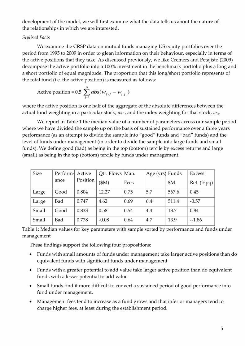
We report in Table 1 the median value of a number of parameters across our sample period

where we have divided the sample up on the basis of sustained performance over a three years

performance (as an attempt to divide the sample into “good” funds and “bad” funds) and the

level of funds under management (in order to divide the sample into large funds and small

funds). We define good (bad) as being in the top (bottom) tercile by excess returns and large

(small) as being in the top (bottom) tercile by funds under management.

Size Perform-

ance

Active

Position

Qtr. Flows

($M)

Man.

Fees

Age (yrs) Funds

$M

Excess

Ret. (%pq)

Large Good 0.804 12.27 0.75 5.7 567.6 0.45

Large Bad 0.747 4.62 0.69 6.4 511.4 -0.57

Small Good 0.833 0.58 0.54 4.4 13.7 0.84

Small Bad 0.778 -0.08 0.64 4.7 13.9 --1.86

Table 1: Median values for key parameters with sample sorted by performance and funds under

management

These findings support the following four propositions:

Funds with small amounts of funds under management take larger active positions than do

equivalent funds with significant funds under management

Funds with a greater potential to add value take larger active position than do equivalent

funds with a lesser potential to add value

Small funds find it more difficult to convert a sustained period of good performance into

fund under management.

Management fees tend to increase as a fund grows and that inferior managers tend to

charge higher fees, at least during the establishment period.

6

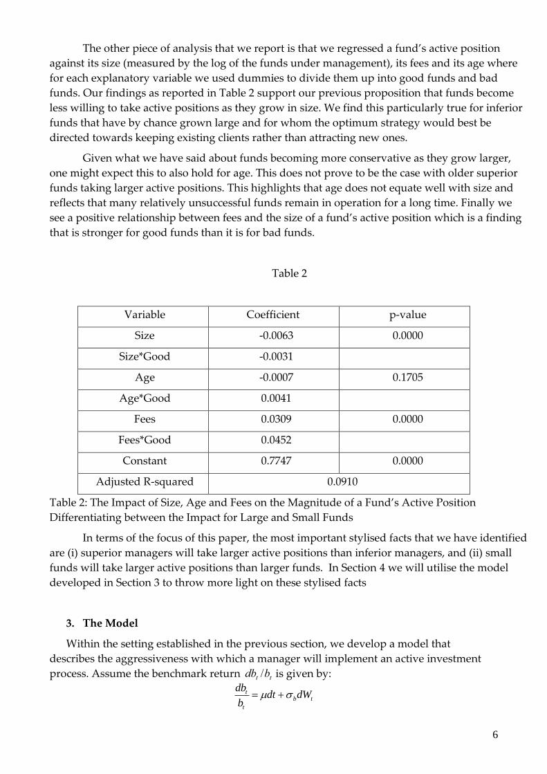
The other piece of analysis that we report is that we regressed a fund’s active position

against its size (measured by the log of the funds under management), its fees and its age where

for each explanatory variable we used dummies to divide them up into good funds and bad

funds. Our findings as reported in Table 2 support our previous proposition that funds become

less willing to take active positions as they grow in size. We find this particularly true for inferior

funds that have by chance grown large and for whom the optimum strategy would best be

directed towards keeping existing clients rather than attracting new ones.

Given what we have said about funds becoming more conservative as they grow larger,

one might expect this to also hold for age. This does not prove to be the case with older superior

funds taking larger active positions. This highlights that age does not equate well with size and

reflects that many relatively unsuccessful funds remain in operation for a long time. Finally we

see a positive relationship between fees and the size of a fund’s active position which is a finding

that is stronger for good funds than it is for bad funds.

Table 2

Variable Coefficient p-value

Size -0.0063 0.0000

Size*Good -0.0031

Age -0.0007 0.1705

Age*Good 0.0041

Fees 0.0309 0.0000

Fees*Good 0.0452

Constant 0.7747 0.0000

Adjusted R-squared 0.0910

Table 2: The Impact of Size, Age and Fees on the Magnitude of a Fund’s Active Position

Differentiating between the Impact for Large and Small Funds

In terms of the focus of this paper, the most important stylised facts that we have identified

are (i) superior managers will take larger active positions than inferior managers, and (ii) small

funds will take larger active positions than larger funds. In Section 4 we will utilise the model

developed in Section 3 to throw more light on these stylised facts

3. The Model

Within the setting established in the previous section, we develop a model that

describes the aggressiveness with which a manager will implement an active investment

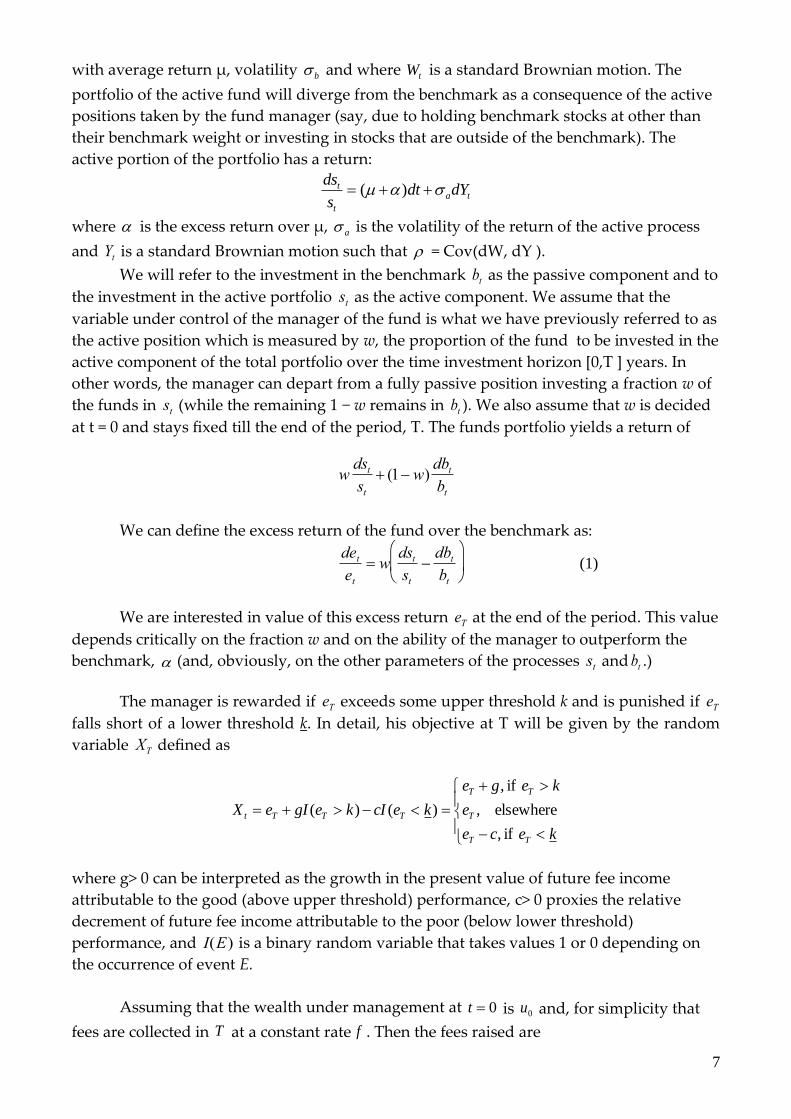
process. Assume the benchmark return

dbt /bt is given by:

tb

t

t dWdtb

db

7

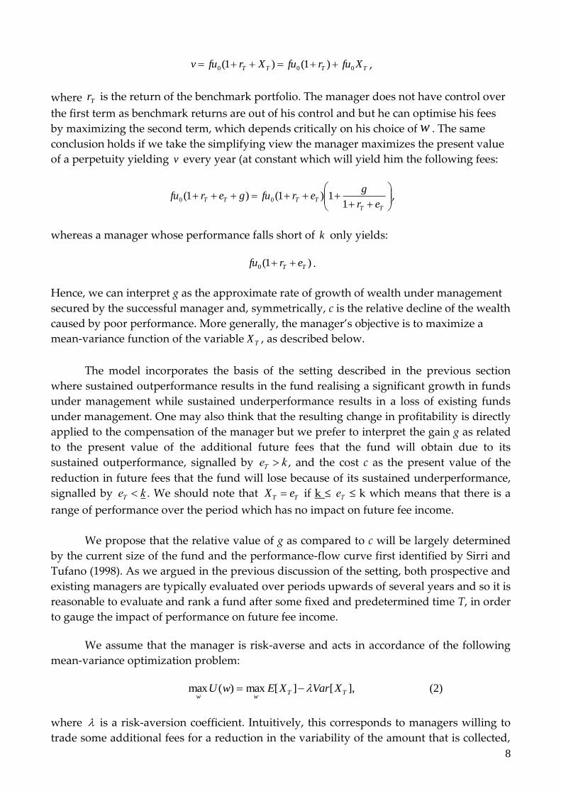
with average return µ, volatility b and where tW is a standard Brownian motion. The

portfolio of the active fund will diverge from the benchmark as a consequence of the active

positions taken by the fund manager (say, due to holding benchmark stocks at other than

their benchmark weight or investing in stocks that are outside of the benchmark). The

active portion of the portfolio has a return:

ta

t

t dYdts

ds )(

where is the excess return over µ, a is the volatility of the return of the active process

and

Yt is a standard Brownian motion such that = Cov(dW, dY ).

We will refer to the investment in the benchmark

bt as the passive component and to

the investment in the active portfolio

st as the active component. We assume that the

variable under control of the manager of the fund is what we have previously referred to as

the active position which is measured by w, the proportion of the fund to be invested in the

active component of the total portfolio over the time investment horizon [0,T ] years. In

other words, the manager can depart from a fully passive position investing a fraction w of

the funds in

st (while the remaining 1 − w remains in

bt ). We also assume that w is decided

at t = 0 and stays fixed till the end of the period, T. The funds portfolio yields a return of

wdst

st (1w)

dbt

bt

We can define the excess return of the fund over the benchmark as:

det

et w

dst

stdbt

bt

(1)

We are interested in value of this excess return

eT at the end of the period. This value

depends critically on the fraction w and on the ability of the manager to outperform the

benchmark,

(and, obviously, on the other parameters of the processes

st and

bt .)

The manager is rewarded if

eT exceeds some upper threshold k and is punished if

eT

falls short of a lower threshold k. In detail, his objective at T will be given by the random

variable

XT defined as

kece

e

kege

kecIkegIeX

TT

T

TT

TTTt

if ,

elsewhere ,

if ,

)()(

where g> 0 can be interpreted as the growth in the present value of future fee income

attributable to the good (above upper threshold) performance, c> 0 proxies the relative

decrement of future fee income attributable to the poor (below lower threshold)

performance, and

I(E) is a binary random variable that takes values 1 or 0 depending on

the occurrence of event E.

Assuming that the wealth under management at 0t is 0u and, for simplicity that

fees are collected in T at a constant rate f . Then the fees raised are

8

TTTT XfurfuXrfuv 000 )1()1( ,

where Tr is the return of the benchmark portfolio. The manager does not have control over

the first term as benchmark returns are out of his control and but he can optimise his fees

by maximizing the second term, which depends critically on his choice of w . The same

conclusion holds if we take the simplifying view the manager maximizes the present value

of a perpetuity yielding v every year (at constant which will yield him the following fees:

TT

TTTTer

gerfugerfu

11)1()1( 00 ,

whereas a manager whose performance falls short of k only yields:

)1(0 TT erfu .

Hence, we can interpret g as the approximate rate of growth of wealth under management

secured by the successful manager and, symmetrically, c is the relative decline of the wealth

caused by poor performance. More generally, the manager’s objective is to maximize a

mean-variance function of the variable TX , as described below.

The model incorporates the basis of the setting described in the previous section

where sustained outperformance results in the fund realising a significant growth in funds

under management while sustained underperformance results in a loss of existing funds

under management. One may also think that the resulting change in profitability is directly

applied to the compensation of the manager but we prefer to interpret the gain g as related

to the present value of the additional future fees that the fund will obtain due to its

sustained outperformance, signalled by

eT k , and the cost c as the present value of the

reduction in future fees that the fund will lose because of its sustained underperformance,

signalled by

eT k . We should note that TT eX if k ≤

eT ≤ k which means that there is a

range of performance over the period which has no impact on future fee income.

We propose that the relative value of g as compared to c will be largely determined

by the current size of the fund and the performance-flow curve first identified by Sirri and

Tufano (1998). As we argued in the previous discussion of the setting, both prospective and

existing managers are typically evaluated over periods upwards of several years and so it is

reasonable to evaluate and rank a fund after some fixed and predetermined time T, in order

to gauge the impact of performance on future fee income.

We assume that the manager is risk-averse and acts in accordance of the following

mean-variance optimization problem:

],[][max)(max TT

wwXVarXEwU (2)

where

is a risk-aversion coefficient. Intuitively, this corresponds to managers willing to

trade some additional fees for a reduction in the variability of the amount that is collected,

9

depending on their personal risk-attitude.

4. Results

This section explores the model of fund behaviour developed in the previous section.

The optimisation problem cannot, to the best of our knowledge, be solved analytically.

Indeed, even if there is a relatively simple expression for the mean of TX , the variance in

(2) involves both the density and the cumulative probability function of normal variables

whose distribution depends on w. Despite the fact that no close-form solution is available

the model is numerically very tractable and optimal active positions under various sets of

assumed values for the parameters can be computed5.

The next subsection will describe the reference parameters. A more general numerical

treatment is then provided in subsection 4.2, where we systematically vary the parameter of

the reference case to explore the effects of asymmetries in the formulation of problem (6).

4.1 A reference example

The model depends on several parameters that describe the passive and active stochastic

processes tt sb , respectively, and other structural exogenous features like g, c and the risk-

aversion coefficient

.

0.05 Avg return of the benchmark

0.00 Avg excess return of the active process

b 0.10 Volatility of the benchmark

a 0.10 Volatility of the active process 0.00 Correlation of active and benchmark

T 3 Time horizon (years)

k 0.05 Upper threshold

k -0.05 Lower threshold

g 0.5 Gain if Te exceeds k at T

c 0.05 Cost if Te is below k at T

0.3 Risk-aversion coefficient

Table 3: Values of the parameters for the reference case. The third column contains a brief

description of each parameter.

The values of the parameters in our example are given in Table 3 and depict a

situation where we have an active fund which might best be described as average (i.e.,

0 ) with both the benchmark and the active component of the portfolio having an

expected annual return of 5% with a volatility of 10%. The two processes are uncorrelated

and the performance of the fund will be evaluated after 3 years. If, at the end of the period,

the fund’s return exceeds that of the benchmark portfolio by 5% (k) or more, TX is

5 The results of this section are obtained using R, available at htpp://cran.rproject.org, making use

of the “integrate” and “optimizatize” functions. The code is available upon request.

10

increased by 5.0g . If, instead, the excess return fall short of the benchmark return by 5%

(k) or more, then c = 0.05 is subtracted to TX . Finally, the fund maximizes a mean-variance

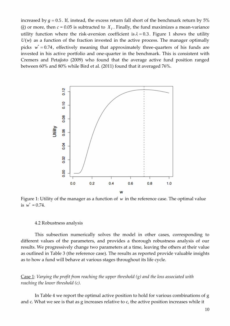
utility function where the risk-aversion coefficient is 3.0 . Figure 1 shows the utility

)(wU as a function of the fraction invested in the active process. The manager optimally

picks 74.0* w , effectively meaning that approximately three-quarters of his funds are

invested in his active portfolio and one-quarter in the benchmark. This is consistent with

Cremers and Petajisto (2009) who found that the average active fund position ranged

between 60% and 80% while Bird et al. (2011) found that it averaged 76%.

Figure 1: Utility of the manager as a function of w in the reference case. The optimal value

is *w = 0.74.

4.2 Robustness analysis

This subsection numerically solves the model in other cases, corresponding to

different values of the parameters, and provides a thorough robustness analysis of our

results. We progressively change two parameters at a time, leaving the others at their value

as outlined in Table 3 (the reference case). The results as reported provide valuable insights

as to how a fund will behave at various stages throughout its life cycle.

Case 1: Varying the profit from reaching the upper threshold (g) and the loss associated with

reaching the lower threshold (c).

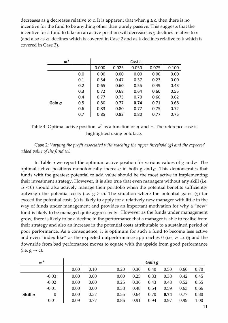
In Table 4 we report the optimal active position to hold for various combinations of g

and c. What we see is that as g increases relative to c, the active position increases while it

11

decreases as g decreases relative to c. It is apparent that when g ≤ c, then there is no

incentive for the fund to be anything other than purely passive. This suggests that the

incentive for a fund to take on an active position will decrease as g declines relative to c

(and also as declines which is covered in Case 2 and as k declines relative to k which is

covered in Case 3).

w* Cost c

0.000 0.025 0.050 0.075 0.100

0.0 0.00 0.00 0.00 0.00 0.00 0.1 0.54 0.47 0.37 0.23 0.00 0.2 0.65 0.60 0.55 0.49 0.43 0.3 0.72 0.68 0.64 0.60 0.55 0.4 0.77 0.73 0.70 0.66 0.62

Gain g 0.5 0.80 0.77 0.74 0.71 0.68 0.6 0.83 0.80 0.77 0.75 0.72 0.7 0.85 0.83 0.80 0.77 0.75

Table 4: Optimal active position *w as a function of g and c . The reference case is

highlighted using boldface.

Case 2: Varying the profit associated with reaching the upper threshold (g) and the expected

added value of the fund (α)

In Table 5 we report the optimum active position for various values of g and

. The

optimal active positions monotonically increase in both g and

. This demonstrates that

funds with the greatest potential to add value should be the most active in implementing

their investment strategy. However, it is also true that even managers without any skill (i.e.

< 0) should also actively manage their portfolio when the potential benefits sufficiently

outweigh the potential costs (i.e. g > c). The situation where the potential gains (g) far

exceed the potential costs (c) is likely to apply for a relatively new manager with little in the

way of funds under management and provides an important motivation for why a “new”

fund is likely to be managed quite aggressively. However as the funds under management

grow, there is likely to be a decline in the performance that a manager is able to realise from

their strategy and also an increase in the potential costs attributable to a sustained period of

poor performance. As a consequence, it is optimum for such a fund to become less active

and even “index like” as the expected outperformance approaches 0 (i.e.

0) and the

downside from bad performance moves to equate with the upside from good performance

(i.e. g c).

w* Gain g

0.00 0.10 0.20 0.30 0.40 0.50 0.60 0.70

-0.03 0.00 0.00 0.00 0.25 0.33 0.38 0.42 0.45

-0.02 0.00 0.00 0.25 0.36 0.43 0.48 0.52 0.55

-0.01 0.00 0.00 0.38 0.48 0.54 0.59 0.63 0.66

Skill α 0 0.00 0.37 0.55 0.64 0.70 0.74 0.77 0.80

0.01 0.09 0.77 0.86 0.91 0.94 0.97 0.99 1.00

12

0.02 1.00 1.00 1.00 1.00 1.00 1.00 1.00 1.00

0.03 1.00 1.00 1.00 1.00 1.00 1.00 1.00 1.00

Table 5: Optimal active position *w as a function of g and

. The reference case is

highlighted using boldface.

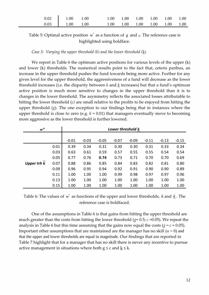
Case 3: Varying the upper threshold (k) and the lower threshold (k).

We report in Table 6 the optimum active positions for various levels of the upper (k)

and lower (k) thresholds. The numerical results point to the fact that, ceteris paribus, an

increase in the upper threshold pushes the fund towards being more active. Further for any

given level for the upper threshold, the aggressiveness of a fund will decrease as the lower

threshold increases (i.e. the disparity between k and k increases) but that a fund’s optimum

active position is much more sensitive to changes in the upper threshold than it is to

changes in the lower threshold. The asymmetry reflects the associated losses attributable to

hitting the lower threshold (c) are small relative to the profits to be enjoyed from hitting the

upper threshold (g). The one exception to our findings being that in instances where the

upper threshold is close to zero (e.g. k = 0.01) that managers eventually move to becoming

more aggressive as the lower threshold is further lowered.

w* Lower threshold

-0.01 -0.03 -0.05 -0.07 -0.09 -0.11 -0.13 -0.15

0.01 0.39 0.34 0.31 0.30 0.30 0.31 0.33 0.34

0.03 0.63 0.61 0.59 0.57 0.55 0.55 0.54 0.54

0.05 0.77 0.76 0.74 0.73 0.71 0.70 0.70 0.69

Upper trh 0.07 0.88 0.86 0.85 0.84 0.83 0.82 0.81 0.80

0.09 0.96 0.95 0.94 0.92 0.91 0.90 0.90 0.89

0.11 1.00 1.00 1.00 0.99 0.98 0.97 0.97 0.96

0.13 1.00 1.00 1.00 1.00 1.00 1.00 1.00 1.00

0.15 1.00 1.00 1.00 1.00 1.00 1.00 1.00 1.00

Table 6: The values of *w as functions of the upper and lower thresholds, k and k . The

reference case is boldfaced.

One of the assumptions in Table 6 is that gains from hitting the upper threshold are

much greater than the costs from hitting the lower threshold (g= 0.5; c =0.05). We repeat the

analysis in Table 6 but this time assuming that the gains now equal the costs (g = c = 0.05).

Important other assumptions that are maintained are the manager has no skill (α = 0) and

that the upper and lower thresholds are equal in magnitude. Our findings that are reported in

Table 7 highlight that for a manager that has no skill there is never any incentive to pursue

active management in situations where both g ≤ c and k ≤ k.

13

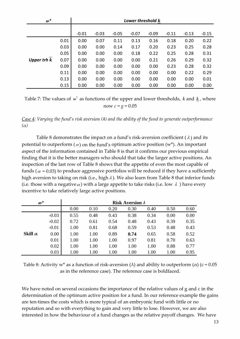
w* Lower threshold

-0.01 -0.03 -0.05 -0.07 -0.09 -0.11 -0.13 -0.15

0.01 0.00 0.07 0.11 0.13 0.16 0.18 0.20 0.22

0.03 0.00 0.00 0.14 0.17 0.20 0.23 0.25 0.28

0.05 0.00 0.00 0.00 0.18 0.22 0.25 0.28 0.31

Upper trh 0.07 0.00 0.00 0.00 0.00 0.21 0.26 0.29 0.32

0.09 0.00 0.00 0.00 0.00 0.00 0.23 0.28 0.32

0.11 0.00 0.00 0.00 0.00 0.00 0.00 0.22 0.29

0.13 0.00 0.00 0.00 0.00 0.00 0.00 0.00 0.01

0.15 0.00 0.00 0.00 0.00 0.00 0.00 0.00 0.00

Table 7: The values of *w as functions of the upper and lower thresholds, k and k , where

now c = g = 0.05

Case 4: Varying the fund’s risk aversion (λ) and the ability of the fund to generate outperformance

(α)

Table 8 demonstrates the impact on a fund’s risk-aversion coefficient (

) and its

potential to outperform (

) on the fund’s optimum active position (w*). An important

aspect of the information contained in Table 8 is that it confirms our previous empirical

finding that it is the better managers who should that take the larger active positions. An

inspection of the last row of Table 8 shows that the appetite of even the most capable of

funds (

= 0.03) to produce aggressive portfolios will be reduced if they have a sufficiently

high aversion to taking on risk (i.e., high

). We also learn from Table 8 that inferior funds

(i.e. those with a negative

) with a large appetite to take risks (i.e. low ) have every

incentive to take relatively large active positions.

w* Risk Aversion λ

0.00 0.10 0.20 0.30 0.40 0.50 0.60

-0.03 0.55 0.48 0.43 0.38 0.34 0.00 0.00

-0.02 0.72 0.61 0.54 0.48 0.43 0.39 0.35

-0.01 1.00 0.81 0.68 0.59 0.53 0.48 0.43

Skill α 0.00 1.00 1.00 0.89 0.74 0.65 0.58 0.52

0.01 1.00 1.00 1.00 0.97 0.81 0.70 0.63

0.02 1.00 1.00 1.00 1.00 1.00 0.88 0.77

0.03 1.00 1.00 1.00 1.00 1.00 1.00 0.95

Table 8: Activity w* as a function of risk-aversion (λ) and ability to outperform (α) (c = 0.05

as in the reference case). The reference case is boldfaced.

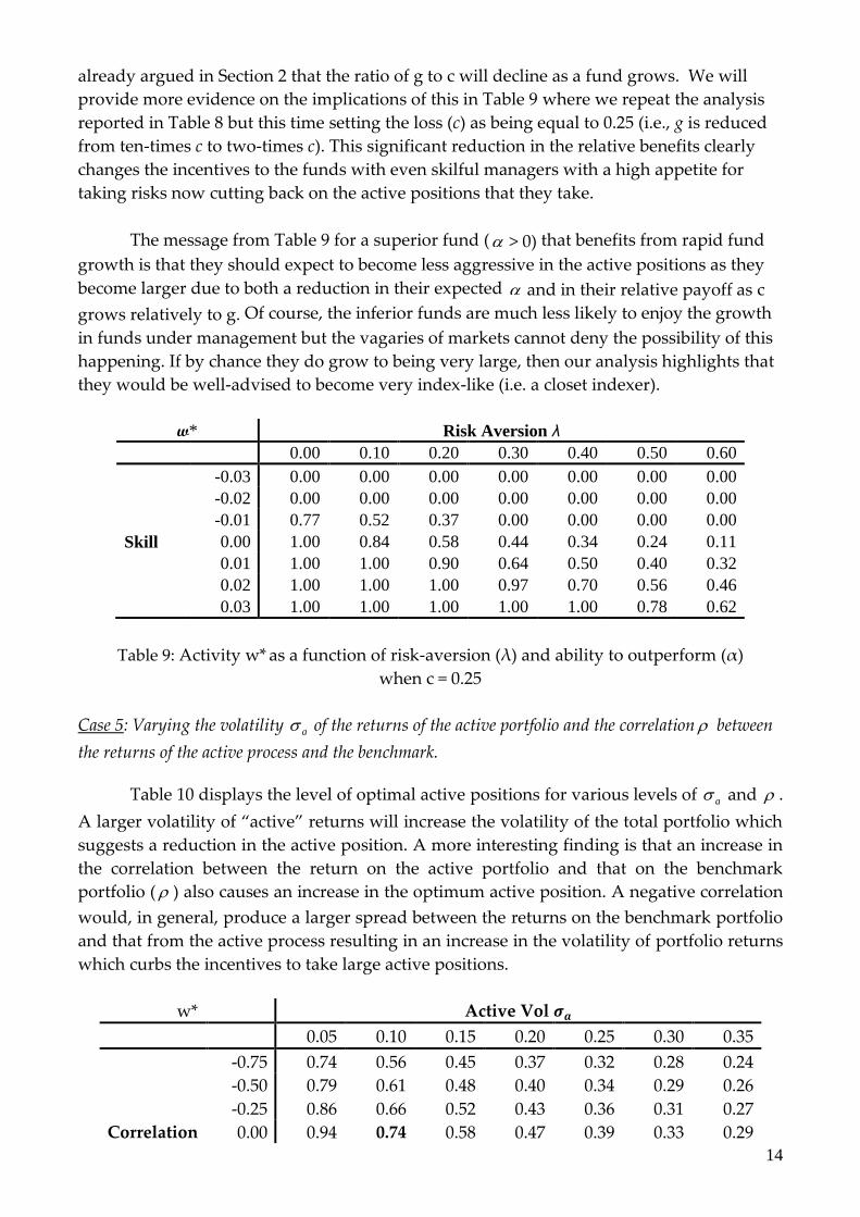
We have noted on several occasions the importance of the relative values of g and c in the

determination of the optimum active position for a fund. In our reference example the gains

are ten-times the costs which is more typical of an embryonic fund with little or no

reputation and so with everything to gain and very little to lose. However, we are also

interested in how the behaviour of a fund changes as the relative payoff changes. We have

14

already argued in Section 2 that the ratio of g to c will decline as a fund grows. We will

provide more evidence on the implications of this in Table 9 where we repeat the analysis

reported in Table 8 but this time setting the loss (c) as being equal to 0.25 (i.e., g is reduced

from ten-times c to two-times c). This significant reduction in the relative benefits clearly

changes the incentives to the funds with even skilful managers with a high appetite for

taking risks now cutting back on the active positions that they take.

The message from Table 9 for a superior fund (

> 0) that benefits from rapid fund

growth is that they should expect to become less aggressive in the active positions as they

become larger due to both a reduction in their expected

and in their relative payoff as c

grows relatively to g. Of course, the inferior funds are much less likely to enjoy the growth

in funds under management but the vagaries of markets cannot deny the possibility of this

happening. If by chance they do grow to being very large, then our analysis highlights that

they would be well-advised to become very index-like (i.e. a closet indexer).

w* Risk Aversion λ

0.00 0.10 0.20 0.30 0.40 0.50 0.60

-0.03 0.00 0.00 0.00 0.00 0.00 0.00 0.00

-0.02 0.00 0.00 0.00 0.00 0.00 0.00 0.00

-0.01 0.77 0.52 0.37 0.00 0.00 0.00 0.00

Skill 0.00 1.00 0.84 0.58 0.44 0.34 0.24 0.11

0.01 1.00 1.00 0.90 0.64 0.50 0.40 0.32

0.02 1.00 1.00 1.00 0.97 0.70 0.56 0.46

0.03 1.00 1.00 1.00 1.00 1.00 0.78 0.62

Table 9: Activity w* as a function of risk-aversion (λ) and ability to outperform (α)

when c = 0.25

Case 5: Varying the volatility a of the returns of the active portfolio and the correlation between

the returns of the active process and the benchmark.

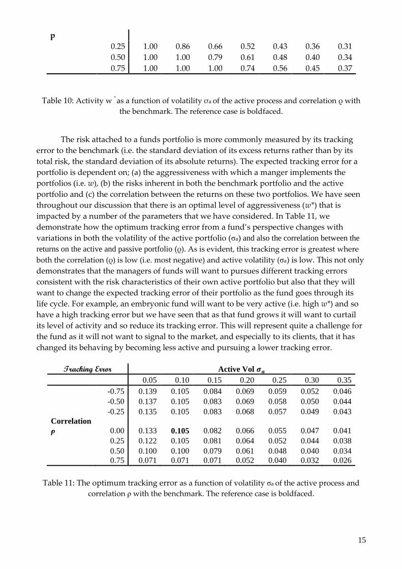
Table 10 displays the level of optimal active positions for various levels of a and .

A larger volatility of “active” returns will increase the volatility of the total portfolio which

suggests a reduction in the active position. A more interesting finding is that an increase in

the correlation between the return on the active portfolio and that on the benchmark

portfolio ( ) also causes an increase in the optimum active position. A negative correlation

would, in general, produce a larger spread between the returns on the benchmark portfolio

and that from the active process resulting in an increase in the volatility of portfolio returns

which curbs the incentives to take large active positions.

w* Active Vol

0.05 0.10 0.15 0.20 0.25 0.30 0.35

-0.75 0.74 0.56 0.45 0.37 0.32 0.28 0.24

-0.50 0.79 0.61 0.48 0.40 0.34 0.29 0.26

-0.25 0.86 0.66 0.52 0.43 0.36 0.31 0.27

Correlation 0.00 0.94 0.74 0.58 0.47 0.39 0.33 0.29

15

p

0.25 1.00 0.86 0.66 0.52 0.43 0.36 0.31

0.50 1.00 1.00 0.79 0.61 0.48 0.40 0.34

0.75 1.00 1.00 1.00 0.74 0.56 0.45 0.37

Table 10: Activity w ∗

as a function of volatility σa of the active process and correlation ρ with

the benchmark. The reference case is boldfaced.

The risk attached to a funds portfolio is more commonly measured by its tracking

error to the benchmark (i.e. the standard deviation of its excess returns rather than by its

total risk, the standard deviation of its absolute returns). The expected tracking error for a

portfolio is dependent on; (a) the aggressiveness with which a manger implements the

portfolios (i.e. w), (b) the risks inherent in both the benchmark portfolio and the active

portfolio and (c) the correlation between the returns on these two portfolios. We have seen

throughout our discussion that there is an optimal level of aggressiveness (w*) that is

impacted by a number of the parameters that we have considered. In Table 11, we

demonstrate how the optimum tracking error from a fund’s perspective changes with

variations in both the volatility of the active portfolio (σa) and also the correlation between the

returns on the active and passive portfolio (ρ). As is evident, this tracking error is greatest where

both the correlation (ρ) is low (i.e. most negative) and active volatility (σa) is low. This not only

demonstrates that the managers of funds will want to pursues different tracking errors

consistent with the risk characteristics of their own active portfolio but also that they will

want to change the expected tracking error of their portfolio as the fund goes through its

life cycle. For example, an embryonic fund will want to be very active (i.e. high w*) and so

have a high tracking error but we have seen that as that fund grows it will want to curtail

its level of activity and so reduce its tracking error. This will represent quite a challenge for

the fund as it will not want to signal to the market, and especially to its clients, that it has

changed its behaving by becoming less active and pursuing a lower tracking error.

Tracking Error Active Vol

0.05 0.10 0.15 0.20 0.25 0.30 0.35

-0.75 0.139 0.105 0.084 0.069 0.059 0.052 0.046

-0.50 0.137 0.105 0.083 0.069 0.058 0.050 0.044

-0.25 0.135 0.105 0.083 0.068 0.057 0.049 0.043

Correlation

p 0.00 0.133 0.105 0.082 0.066 0.055 0.047 0.041

0.25 0.122 0.105 0.081 0.064 0.052 0.044 0.038

0.50 0.100 0.100 0.079 0.061 0.048 0.040 0.034

0.75 0.071 0.071 0.071 0.052 0.040 0.032 0.026

Table 11: The optimum tracking error as a function of volatility σa of the active process and

correlation ρ with the benchmark. The reference case is boldfaced.

16

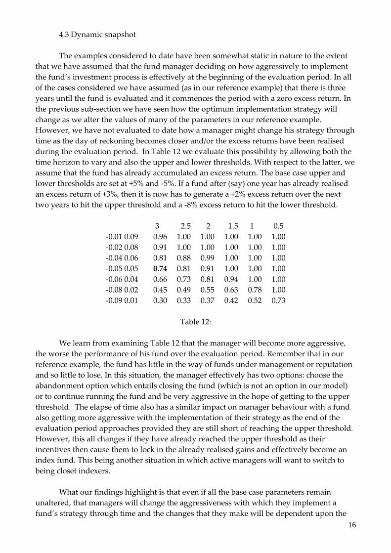
4.3 Dynamic snapshot

The examples considered to date have been somewhat static in nature to the extent

that we have assumed that the fund manager deciding on how aggressively to implement

the fund’s investment process is effectively at the beginning of the evaluation period. In all

of the cases considered we have assumed (as in our reference example) that there is three

years until the fund is evaluated and it commences the period with a zero excess return. In

the previous sub-section we have seen how the optimum implementation strategy will

change as we alter the values of many of the parameters in our reference example.

However, we have not evaluated to date how a manager might change his strategy through

time as the day of reckoning becomes closer and/or the excess returns have been realised

during the evaluation period. In Table 12 we evaluate this possibility by allowing both the

time horizon to vary and also the upper and lower thresholds. With respect to the latter, we

assume that the fund has already accumulated an excess return. The base case upper and

lower thresholds are set at +5% and -5%. If a fund after (say) one year has already realised

an excess return of +3%, then it is now has to generate a +2% excess return over the next

two years to hit the upper threshold and a -8% excess return to hit the lower threshold.

3 2.5 2 1.5 1 0.5

-0.01 0.09 0.96 1.00 1.00 1.00 1.00 1.00

-0.02 0.08 0.91 1.00 1.00 1.00 1.00 1.00

-0.04 0.06 0.81 0.88 0.99 1.00 1.00 1.00

-0.05 0.05 0.74 0.81 0.91 1.00 1.00 1.00

-0.06 0.04 0.66 0.73 0.81 0.94 1.00 1.00

-0.08 0.02 0.45 0.49 0.55 0.63 0.78 1.00

-0.09 0.01 0.30 0.33 0.37 0.42 0.52 0.73

Table 12:

We learn from examining Table 12 that the manager will become more aggressive,

the worse the performance of his fund over the evaluation period. Remember that in our

reference example, the fund has little in the way of funds under management or reputation

and so little to lose. In this situation, the manager effectively has two options: choose the

abandonment option which entails closing the fund (which is not an option in our model)

or to continue running the fund and be very aggressive in the hope of getting to the upper

threshold. The elapse of time also has a similar impact on manager behaviour with a fund

also getting more aggressive with the implementation of their strategy as the end of the

evaluation period approaches provided they are still short of reaching the upper threshold.

However, this all changes if they have already reached the upper threshold as their

incentives then cause them to lock in the already realised gains and effectively become an

index fund. This being another situation in which active managers will want to switch to

being closet indexers.

What our findings highlight is that even if all the base case parameters remain

unaltered, that managers will change the aggressiveness with which they implement a

fund’s strategy through time and the changes that they make will be dependent upon the

17

previous performance of the fund. We have seen in the reference example that it is optimal

for a manager to initially place 74% of his funds in his active portfolio. Assuming that the

fund achieves benchmark performance in the first year, then the manager will increase this

allocation to the active fund to 91%. However, if the fund outperforms the benchmark by

3% in the first year then the manager will reduce the allocation to the active portfolio to

55%

5. A Life-Cycle Example

In this section of the paper we draw upon the previous analysis to provide a specific

example of the behaviour of managers at different stages in their life cycle. In particular, we

consider:

A boutique manager who has little in the way of funds under management. Such a

manager has little to lose as a result of a sustained period of underperformance (i.e. a

low c in our model) and little to prevent them being able to realise the full potential

of their investment process (i.e. no erosion in the ά in our model)

A “mid-cycle” manager who either because of skill or luck has been able to generate a

sustained period of outperformance. As a consequence this manager is in the early

stages of a growth spurt in funds under management resulting in the manager now

having something to lose both in terms of funds being managed and a growing

reputation (i.e. a rising c in our model). Also the growing funds being managed are

beginning to cause a drag on performance and so the manager is already finding

erosion in the potential to add value (i.e. a reduction in ά)6.

A mature manager who again because of skill or luck has been able to generate

sufficient good performance to attract a large amount of funds. As a result the

potential exist for the fund to lose a large amount of funds under management and

the level of funds under management is now making it increasing more difficult for

him to realise his potential to outperform (i.e. a even greater reduction in his ά)

We further consider two managers with differing investment capabilities. We have a

good manager whose investment process is expected to generate positive alphas in the long

run but that this positive alpha will erode with significant growth in his funds under

management. We also have a bad manager whose process is expected to generate negative

alphas in the long run. However, it is far from impossible for our bad manager to generate

sufficiently good investment performance to advance to the mid-cycle, if not mature, stage

of the cycle. For example, a manager with an expected annualised alpha of -1.5% with a

standard deviation of 10% has a 30.0% probability of outperforming by 5% over three years,

and a 27.7% probability of outperforming by 5% over five years. Finally, we assume that the

expected performance (ά) of the bad manager does not erode in the event that he does

significantly grow funds under management.

We use the same procedures as in Section 4 to calculate the optimal active position

(w*) for the two managers at each of the three stages in the cycle largely using the reference

example assumptions as set out in Table 3. The exceptions to these base assumptions are set

6 The point at which these constraints will begin to take effect will vary from market to market largely determined by the

size of the market.

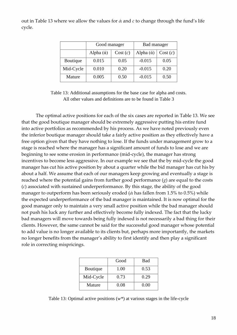
18

out in Table 13 where we allow the values for ά and c to change through the fund’s life

cycle.

Good manager Bad manager

Alpha (ά) Cost (c) Alpha (ά) Cost (c)

Boutique 0.015 0.05 -0.015 0.05

Mid-Cycle 0.010 0.20 -0.015 0.20

Mature 0.005 0.50 -0.015 0.50

Table 13: Additional assumptions for the base case for alpha and costs.

All other values and definitions are to be found in Table 3

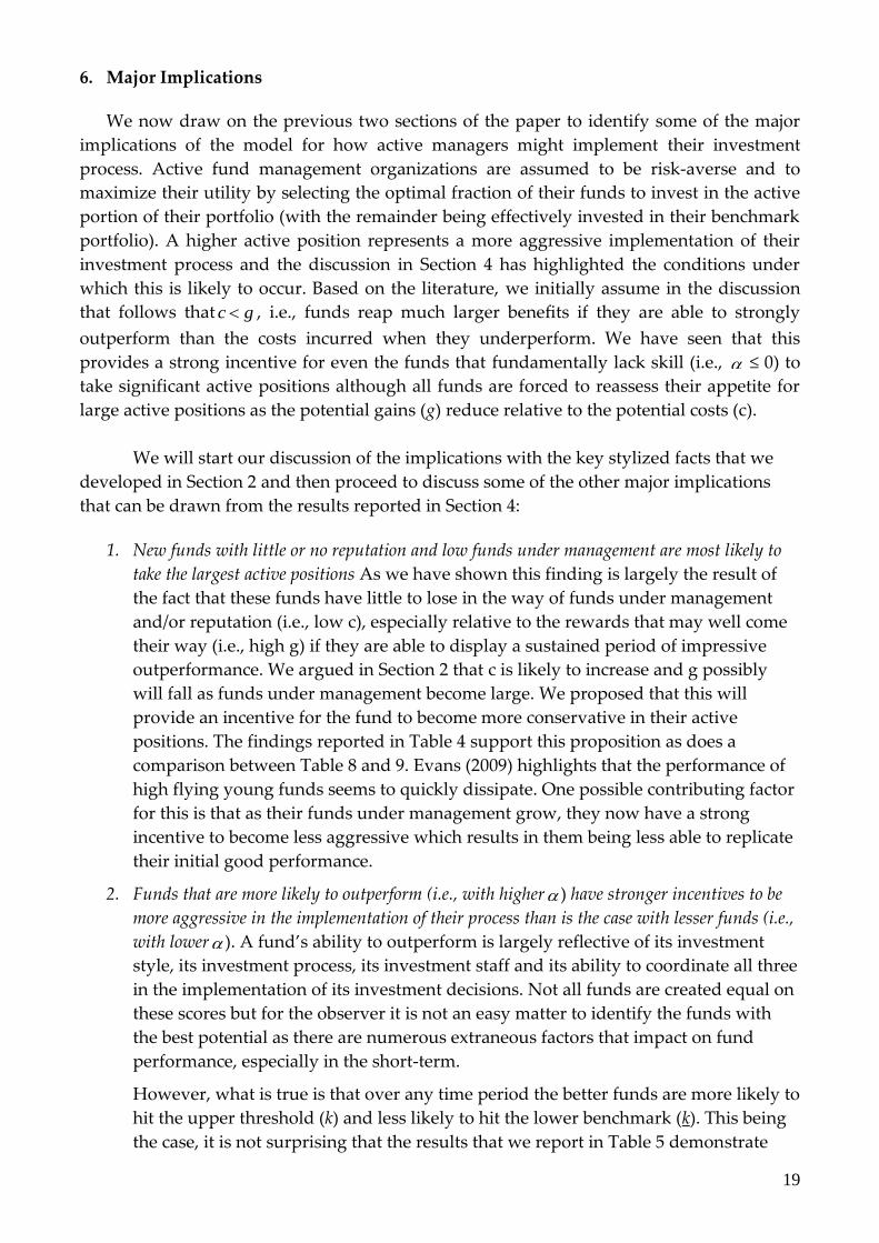
The optimal active positions for each of the six cases are reported in Table 13. We see

that the good boutique manager should be extremely aggressive putting his entire fund

into active portfolios as recommended by his process. As we have noted previously even

the inferior boutique manager should take a fairly active position as they effectively have a

free option given that they have nothing to lose. If the funds under management grow to a

stage is reached where the manager has a significant amount of funds to lose and we are

beginning to see some erosion in performance (mid-cycle), the manager has strong

incentives to become less aggressive. In our example we see that the by mid-cycle the good

manager has cut his active position by about a quarter while the bid manager has cut his by

about a half. We assume that each of our managers keep growing and eventually a stage is

reached where the potential gains from further good performance (g) are equal to the costs

(c) associated with sustained underperformance. By this stage, the ability of the good

manager to outperform has been seriously eroded (ά has fallen from 1.5% to 0.5%) while

the expected underperformance of the bad manager is maintained. It is now optimal for the

good manager only to maintain a very small active position while the bad manager should

not push his luck any further and effectively become fully indexed. The fact that the lucky

bad managers will move towards being fully indexed is not necessarily a bad thing for their

clients. However, the same cannot be said for the successful good manager whose potential

to add value is no longer available to its clients but, perhaps more importantly, the markets

no longer benefits from the manager’s ability to first identify and then play a significant

role in correcting mispricings.

Good Bad

Boutique 1.00 0.53

Mid-Cycle 0.73 0.29

Mature 0.08 0.00

Table 13: Optimal active positions (w*) at various stages in the life-cycle

19

6. Major Implications

We now draw on the previous two sections of the paper to identify some of the major

implications of the model for how active managers might implement their investment

process. Active fund management organizations are assumed to be risk-averse and to

maximize their utility by selecting the optimal fraction of their funds to invest in the active

portion of their portfolio (with the remainder being effectively invested in their benchmark

portfolio). A higher active position represents a more aggressive implementation of their

investment process and the discussion in Section 4 has highlighted the conditions under

which this is likely to occur. Based on the literature, we initially assume in the discussion

that follows that gc , i.e., funds reap much larger benefits if they are able to strongly

outperform than the costs incurred when they underperform. We have seen that this

provides a strong incentive for even the funds that fundamentally lack skill (i.e.,

≤ 0) to

take significant active positions although all funds are forced to reassess their appetite for

large active positions as the potential gains (g) reduce relative to the potential costs (c).

We will start our discussion of the implications with the key stylized facts that we

developed in Section 2 and then proceed to discuss some of the other major implications

that can be drawn from the results reported in Section 4:

1. New funds with little or no reputation and low funds under management are most likely to

take the largest active positions As we have shown this finding is largely the result of

the fact that these funds have little to lose in the way of funds under management

and/or reputation (i.e., low c), especially relative to the rewards that may well come

their way (i.e., high g) if they are able to display a sustained period of impressive

outperformance. We argued in Section 2 that c is likely to increase and g possibly

will fall as funds under management become large. We proposed that this will

provide an incentive for the fund to become more conservative in their active

positions. The findings reported in Table 4 support this proposition as does a

comparison between Table 8 and 9. Evans (2009) highlights that the performance of

high flying young funds seems to quickly dissipate. One possible contributing factor

for this is that as their funds under management grow, they now have a strong

incentive to become less aggressive which results in them being less able to replicate

their initial good performance.

2. Funds that are more likely to outperform (i.e., with higher

) have stronger incentives to be

more aggressive in the implementation of their process than is the case with lesser funds (i.e.,

with lower

). A fund’s ability to outperform is largely reflective of its investment

style, its investment process, its investment staff and its ability to coordinate all three

in the implementation of its investment decisions. Not all funds are created equal on

these scores but for the observer it is not an easy matter to identify the funds with

the best potential as there are numerous extraneous factors that impact on fund

performance, especially in the short-term.

However, what is true is that over any time period the better funds are more likely to

hit the upper threshold (k) and less likely to hit the lower benchmark (k). This being

the case, it is not surprising that the results that we report in Table 5 demonstrate

20

that the optimum active position for a fund increases with its potential to outperform

(i.e., funds with a higher

). We see by comparing Tables 8 and 9 that even these

superior funds will reduce their optimum active positions in line with a reduction in

the relative payoffs stemming from a sustained period of outperformance.

One other issue worth contemplating here is whether it is appropriate to assume that

funds that take the more active positions are the superior managers. Studies by

Cremers and Petajisto (2009) and Bird et al (2011) confirm a positive relationship

between the extent of the active positions taken by Funds and their performance

which provides prima facie evidence in support of the proposition that it is the better

managers that are willing to be more aggressive in implementing their strategies.

Other recent studies that provide support for this proposition include Jiang and

Verado (2012) who found that it is the better performing managers who do not herd

with other managers and Kacperczyk and Seru (2007) who found that a negative

association between a fund’s investment performance and the extent to which it

reacted to changes in analysts’ forecast. Overall, the evidence raises the possibility

that managers might be a relatively good judge of the potential of their fund and so

may provide signals via their investment behaviour including their willingness to

take active positions that are useful to investors when choosing funds in which to

invest.

3. It is not only

that has implications for the optimum active positions but also the impact

that the active positions have on the volatility of the portfolio’s performance. We see from

Table 10 that the optimum active position decreases if the volatility a of the active

process increases and/or it is less correlated with the benchmark. While the first of

these findings is not surprising, the second one is less intuitive and is related to our

initial point that it is the impact of the active position on the risk of the whole

portfolio that is important in determining the optimum level of the active position. A

negative correlation increases the spread between the return on the benchmark

portfolio and that on the actual portfolio (benchmark plus active position). This

translates into an increase in the variance of X, which suggests a more conservative

approach to implementing an active strategy.

4. The attitude to risk of the fund management organization (and managers of individual funds)

will play an important role in determining how aggressive they are in implementing the

fund’s investment process. We see from Table 8 (and Table 9) that the more risk-averse

organisations will be more conservative when implementing the investment process

of the fund (i.e., have a lower *w ). The issue of what determines an organizations

level of risk-aversion is very complex but one factor that may impact on a fund’s

aversion to risk is its reputation. The manager of a fund may wish to protect its

reputation by becoming more conservative in the implementation of the process and

so reduce the probability of sustained underperformance7. This could be tested by

observing the differing behaviour of new boutique fund organisations when

implementing their initial products to see if it is affected by the reputation of the

7 Another factor that would impact on behaviour will be the level of funds under management which will also drive a

more conservative approach because it means that they organization has more at risk.

21

promoters of the funds. For example, those managers who are establishing a

boutique after establishing a good reputation while working with a larger manager

will be more conservative than managers of a boutique who have little in the way of

reputation.

One issue that we have not taken up in our discussion is the potential conflict

between those that manage the fund and those that own the organisation offering

the fund. Where the manager(s) does not hold a large proportion of the equity in the

organisation, it is possible that his attitude to risk (

) is much different to that of the

organisation. For example, the organisation might run numerous funds and be more

interested in the risk that a particular fund brings to its whole portfolio of funds.

Thus a conflict may arise between the organisation offering a particular fund and the

manager of that fund in terms of the aggressiveness with which the process is

implemented. This conflict may become a particular problem where a fund is

“required” to become less aggressive as it grows in size due to past good

performance. This is likely to result in a very capable manager becoming dissatisfied

due to being restrained from displaying his full potential. One way of coping with

the conflicts within the organisation is by increasing the remuneration but this may

not be sufficient to always solve the problem with the possible end result that the

manager leaves the fund. Indeed, the manager may leave and set up his own

boutique where he will have unfettered control over the implementation of the

process.

5. The way that movement in the thresholds will impact on the optimum active position. The

proposition in this paper is that sustained out (under) performance will have a

positive (negative) impact on future fund flows. We have chosen to model sustained

outperformance as requiring the fund to outperform by at least a specified amount

(the upper threshold, k) over a particular time period. This is consistent with the

findings of Sirri and Tufano (1998) that beyond some point outperformance results

in a rapid flow of new funds8.

We show in Table 6 that an increase in the magnitude of the lower threshold (k)

typically results in a slight decrease in the optimum active position. We might expect

to find an analogous relationship between changes in the upper threshold (k) and

the optimum active position with an increase in the magnitude of the upper

threshold resulting in a decrease in the optimum active position. However, we find

the opposite to be the case with the optimum active position (w*) actually increasing

as the upper threshold (k) increases. On reflection, this is not such a surprising

finding when one remembers that the assumed gains from outperformance (g) in our

base case are ten-times greater than the costs (c) associated with underperformance.

When we checked to see what happened in cases where g = c (Table 11), we found

that the optimum active position no longer consistently increased as the upper

8 Our assumption of a substantial fund inflow (outflow) if a positive (negative) threshold excess return is realised within a

specified timeframe is a fairly simple representation of the Sirri and Tufano (1998) findings. However, our prime

consideration in building our model is to keep it both simple and realistic. We could have modelled the Sirri and Tufano

findings with respect to the performance/fund flow relationship more precisely but it would not have introduced any

more realism into the model nor would it have altered our findings.

22

threshold is increased. The optimum active position w* does initially increase where

the upper threshold (k) is initially low relative to the lower threshold (k) but then w*

begins to decrease as k approaches k and becomes zero where k ≥ k.

6. When should an active manager become passive? The answer to this question depends on

the skill of the manager (

), the relative payoffs (g cf c) and the level of the

thresholds (k cf k). For a manager with average skill (

= 0), there will never be a

case to be active when g ≤ c and k ≥ k. In other words, there is never the incentive for

such a manager to implement an active portfolio where the expected gains in future

fee income associated with outperformance are either equal or less than the expected

loses in fees associated with underperformance. Of course this is not the case for a

boutique manager with everything to gain and nothing to lose. The boutique

manager will be relatively active when entering the market even if they lack skill. As

we have seen from our example in Section 5, this will all change as a manager begins

to accumulate asset under management with the incentives being for such a manager

to become increasingly less active and possible eventually reach a situation where

the optimum strategy would be to become totally passive

7. Summary

This paper focuses on what has been a largely neglected aspect of the operations of a

funds management organization, how aggressive should it be in implementing its

investment process. Our approach has been to develop a model based on the presumption

that the organization’s objective is to maximise the present value of its future fee income.

We found that the model provides an explanation for certain behaviour that we observe

and in particular:

Those boutique funds with little reputation or funds under management are likely to

be the most aggressive

Those funds with the greatest capabilities to add value ideally also have strong

incentives to be more aggressive than inferior funds.

Importantly, we found that the optimal strategy for funds whose potential is realised

by way of accumulating very large funds under management would be to become “closet”

indexers. We say this because the organization reaches a point where costs associated with

sustained underperformance (c) increase to a level approaching the potential gains

associated with sustained outperformance. Further, the ability of the fund to outperform is

diluted as its funds under management reaches grow in magnitude. We use the words

“closet” indexers as the fund needs to maintain the appearance of still being active because

of the nature of the active mandate with its investors. Otherwise, it runs the risk of losing

funds not because of poor performance but because it has dramatically strayed from the

undertakings that it has given its clients as to how it will manage their funds9.

It is interesting to speculate on some of the possible implications of our findings for

investors. The first insight for investors is that a willingness to take greater active positions,

9 It is interesting to speculate how a fund can become passive without giving the appearance of being passive. The answer

probably lies in neutralising all of its bets on factors that are likely to cause its performance to depart from its benchmark

which will necessarily mean effectively giving up on its process

23

especially in the case of newer funds may be taken as a positive signal as to the capabilities

of these managers. Cremers and Petajisto (2009) have identified that the more active

managers produce better investment outcomes which our model suggests maybe due to the

superior managers being the more aggressive. This suggests that the active positions taken

by a fund might provide a useful signal when trying to differentiate between the skills of

managers. A number of funds of funds have been developed on the premise of constructing

a portfolio of relatively new aggressively managed funds (e.g. the Russell stable of

Opportunity Funds). Tracing the level of a fund’s active position over time might also

provide a good sign of when to divest from a fund. We have suggested that even superior

funds will reduce their level of aggression in line with significant growth in its funds under

management. Observing this as it occurs may provide a good signal of deterioration in the

performance of the fund and so provide an indication as to when an existing manager

should be replaced.

Our findings also have implication for the functioning of markets that rely on

investors identifying and exploiting investment opportunities and so correcting

mispricings. Presumably the funds that realise sustained outperformance are among the

better at identifying exploitable opportunities. The implications of our models are that it is

likely that these funds will become less active over time resulting in the lesser funds

playing a relatively larger role. This possibility combined with a trend towards more

passive investing (index funds and closet indexers) and investment styles that are

disruptive to markets (e.g. momentum) increases concern as to whether we are seeing a

trend towards increasingly less efficient markets (Bird et al., 2011).

In closing, our paper has provided some interesting insights into an oft-neglected

issue: how do funds determine the level of aggression with which they implement their

investment process. In our discussion we have identified a number of areas which would

well benefit from further research.

References

Berk, J. and R. Green (2004), Mutual Fund Flows and Performance in Rational

Markets, Journal of Political Economy, vol.112, pp. 1269 - 2011

Bird, R., P.Pellizzari and D. Yeung (2011), Performance Implications of Active

Management of Mutual Funds. Paul Woolley Centre Working Paper, University of

Technology Sydney

Cremers, M., and A Petajisto (2009), How Active is Your Fund Manager? A New

Measure that Predicts Performance, Review of Financial Studies, Vol. 22, pp. 3329 – 3365.

Evans, R (2010), Mutual Fund Incubation, The Journal of Finance, vol. 65, pp. 1581 –

1611.

Guercio, D., and P. Tkac, P. (2008). Star Power: The Effect of Monrningstar Ratings

on Mutual Fund Flow, Journal of Financial and Quantitative Analysis, Vol. 43, pp 907–936.

24

Jiang, H. and M. Verado (2012), Does Herding Behavior Reveal Skill? An Analysis of

Mutual Fund Performance, London School of Economics Working Paper

Kacperczyk, M. and A. Seru (2007), Fund Manager Use of Public Information: New

Evidence on Managerial Skills. The Journal of Finance, 62, pp. 485 – 528.

Milone, L. and , Pellizzari, P. (2009). Mutual funds flows and the 'Sheriff of

Nottingham' effect, in C. Hernandez, M. Posada, M. and Lopez-Paredes A. (eds.), Artificial

Economics: the Generative Method in Economics, Springer, pp 117-128.

Sirri, E,. and P. Tufano (1998), Costly Search and Mutual Fund Flows, The Journal of

Finance, vol. 53, pp. 1589 – 1622.