arX

iv:a

stro

-ph/

0610

379v

1 1

2 O

ct 2

006

To appear in “Triggering Relativistic Jets (2005)” RevMexAA(SC)

THE STRUCTURE AND DYNAMICS OF GRB JETS

Jonathan Granot1

RESUMEN

El resumen sera traducido al espanol por los editores. There are several lines of evidence which suggestthat the relativistic outflows in gamma-ray bursts (GRBs) are collimated into narrow jets. The jet structurehas important implications for the true energy release and the event rate of GRBs, and can constrain themechanism responsible for the acceleration and collimation of the jet. Nevertheless, the jet structure and itsdynamics as it sweeps up the external medium and decelerates, are not well understood. In this review I discussour current understanding of GRB jets, stressing their structure and dynamics.

ABSTRACT

There are several lines of evidence which suggest that the relativistic outflows in gamma-ray bursts (GRBs) arecollimated into narrow jets. The jet structure has important implications for the true energy release and theevent rate of GRBs, and can constrain the mechanism responsible for the acceleration and collimation of thejet. Nevertheless, the jet structure and its dynamics as it sweeps up the external medium and decelerates, arenot well understood. In this review I discuss our current understanding of GRB jets, stressing their structureand dynamics.

Key Words: GAMMA RAYS: BURSTS — HYDRODYNAMICS — ISM: JETS AND OUTFLOWS —

RELATIVITY

1. INTRODUCTION

Gamma-ray bursts (GRBs) are produced by ahighly relativistic outflow from a compact source(for a comprehensive recent review see Piran 2005).Early GRB models featured a spherical outflow,mainly for simplicity. However, other astrophysicalsources of relativistic outflows such as active galacticnuclei and micro-quasars are in the form of narrowbipolar jets. One might argue (e.g., Rhoads 1997)that, in analogy to other such sources, GRBs mightalso be collimated into narrow jets.

The initial Lorentz factor during the promptgamma-ray emission is very high, Γ0 ∼

> 100, andtherefore we observe emission mainly from very smallangles, θ ∼

< Γ−10 ∼

< 10−2 rad, relative to our line ofsight. This is a result of relativistic beaming (i.e.aberration of light), an effect of special relativity,which causes an emission that is roughly isotropicin the rest frame of the emitting fluid (as is gener-ally expected under most circumstances) to be con-centrated mostly within an angle of Γ−1 around itsdirection of motion in the lab frame, where Γ ≫ 1is the Lorentz factor of the emitting fluid in the labframe. For this reason, the prompt gamma-ray emis-sion probes a region of solid angle ∼ πΓ−2

0 , or a frac-tion ∼ Γ−2

0 /4 ∼ 10−7 − 10−4.5 of the total solid an-gle, and cannot tell us whether the outflow occupies

1KIPAC, Stanford University, CA, USA.

a larger solid angle.

Therefore, more direct evidence in favor of jetsin GRBs had to await the discovery of afterglowemission in the X-ray (Costa et al. 1997), opti-cal (van Paradijs et al. 1997), and radio (Frail et al.1997), that lasts for days, weeks, and months, respec-tively, after the GRB. The afterglow is believed tobe synchrotron emission from the shocked externalmedium. As the relativistic outflow expands out-wards it sweeps up the surrounding medium anddrives a strong relativistic shock into it, called theforward shock, while the ejecta are decelerated bya reverse shock. Eventually, most of the energyis transfered to the shocked external medium be-hind the forward shock, and the flow approaches aspherical self-similar evolution (Blandford & McKee1976), gradually decelerating as it sweeps up the ex-ternal medium.

This is valid not only for an initially sphericaloutflow, but also for the interior of a jet with anangular size larger than Γ−1

0 (as appears to be thecase for GRB jets, e.g. Panaitescu & Kumar 2002),as long as Γ−1 remains smaller than the angular sizeof the jet and the interior of the jet is out of causalcontact with its edges (i.e. before the jet break time).Therefore, before the jet break time the isotropicequivalent energy of the jet, Eiso, is relevant (both forits dynamics and for the resulting emission), while

1

2 GRANOT

at very late times as the jet becomes sub-relativisticand approaches spherical symmetry its true energy,E, is relevant. In the intermediate regime things aremore complicated, and are discussed in this review.

The forward shock is responsible for the longlived afterglow emission, while the reverse shock pro-duces a shorter lived emission, that peaks in theoptical or NIR on a time-scale of tens of seconds,when the reverse shock crosses the shell of ejecta (the“optical flash”, e.g. Akerlof et al. 1999; Sari & Piran1999a,b; Meszaros & Rees 1999). The shocked out-flow gradually cools adiabatically and the peak ofits emission shifts to lower frequencies, until afterabout a day it peaks in the radio (the “radio flare”Kulkarni et al. 1999b; Frail et al. 2000; Berger et al.2003a). During the afterglow, the Lorentz factor Γof the emitting shocked external medium decreaseswith time as it accumulates more mass, causing thevisible region of θ ∼

< Γ−1 around the line of sightto increase with time. This enables us to probe thestructure of the outflow over increasingly larger an-gular scales.

Different lines of evidence suggest that the rel-ativistic outflows in GRBs are collimated into nar-row jets. A compelling, although somewhat indi-rect, argument comes from the very high values forthe energy output in gamma rays assuming isotropicemission, Eγ,iso, that are inferred for GRBs withknown redshifts, z, which approach and in one case(GRB 991023) even exceed M⊙c2. Such extreme en-ergies in an ultra-relativistic outflow are hard to pro-duce in models involving stellar mass progenitors. Ifthe outflow is collimated into a narrow jet (or bipolarjets) that occupies a small fraction, fb ≪ 1, of thetotal solid angle, then the strong relativistic beamingdue to the very high initial Lorentz factor (Γ0 ∼

> 100)causes the emitted gamma rays to be similarly col-limated. This reduces the true energy output ingamma rays by a factor of f−1

b to Eγ = fbEγ,iso,thus significantly reducing the energy requirements.

Estimates of the energy in the afterglowshock from late time radio observations whenthe flow is only mildly relativistic and starts toapproach spherical symmetry (often called “ra-dio calorimetry”; Frail, Waxman & Kulkarni 2000;Berger, Kulkarni & Frail 2004; Frail et al. 2005) typ-ically yield Ek ∼ 1051.5 erg which lends some sup-port for the true energy being significantly smallerthan Eγ,iso. One should keep in mind, however, thatthese are only approximate lower limits on the trueafterglow energy, and the latter can in principle bemuch higher (see, e.g., Eichler & Waxman 2005).

Furthermore, there is good (spectroscopic) ev-

idence that at least some GRBs of the long-softclass occur together (to within a few days) witha core collapse supernova of Type Ic (Stanek et al.2003; Hjorth et al. 2003). In such cases the averageLorentz factor must be 〈Γ〉 ∼

< 2 for a spherical explo-sion, since the accreted mass does not significantlyexceed the ejected mass, and only a fraction of therest energy of the former can provide the kinetic en-ergy for the latter. Therefore, only a small fraction ofthe ejected mass can reach Γ ∼

> 100 which is requiredin order to power the GRB, and hydrodynamic anal-ysis (Tan, Matzner & McKee 2001; Perna & Vietri2002) shows that it would carry a small fraction ofthe total energy which is insufficient to account forthe high end of the observed values of Eγ,iso. For ajet the ejected mass can be much smaller than theaccreted mass so that 〈Γ〉 ≫ 1 is possible, in addi-tion to the smaller Eγ that is implied by the sameobserved Eγ,iso.

A more direct line of evidence in favor ofa narrowly collimated outflow comes from achro-matic breaks seen in the afterglow light curves ofmany GRBs (Fruchter et al. 1999; Kulkarni et al.1999a; Harrison et al. 1999; Stanek et al. 1999, 2001;Berger et al. 2000; Halpern et al. 2000; Price et al.2001; Sagar et al. 2001; Jensen et al. 2001). In fact,such a “jet break” in the afterglow light curve waspredicted before it was detected (Rhoads 1997, 1999;Sari, Piran & Halpern 1999). The cause of the jetbreak in the light curve is discussed in §2.6.

The properties of GRB jets are of fundamentalimportance since they pertain to the GRB energy re-lease, event rate, and the progenitor model throughits ability to produce a particular jet structure. Inparticular, a good understanding of the jet struc-ture and dynamics are crucial in order to reliablyaddress these vital issues. This review focuses onthe dynamics of the jet as it sweeps up the exter-nal medium and decelerates (§2) and on its angularstructure (§3), stressing the constraints that may bederived from various observations. The conclusionsare discussed in §4.

2. THE JET DYNAMICS

This section begins by presenting three differentapproaches to the calculation of the jet dynamics, inorder of increasing complexity: semi-analytic models(§ 2.1), simplifying the dynamical equations by inte-grating over the radial profile of the jet (§ 2.2), andfull hydrodynamic simulations (§ 2.3). The main re-sults of the different approaches are described andcompared. Next (§ 2.4) there is a brief descriptionof the typical assumptions that are made in order to

JETS IN GAMMA-RAY BURSTS 3

calculate the afterglow emission. The afterglow im-age is discussed in § 2.5 along with potential methodsfor resolving it and constraining its angular size, aswell as how its morphology and the evolution of itssize may help us learn about the jet dynamics andthe external density profile. Finally, the cause of thejet break in the afterglow light curve is discussed in§ 2.6.

2.1. Simple Semi-Analytic Models

The first approach that had been adoptedfor calculating the jet dynamics was using asimple semi-analytic model (Rhoads 1997, 1999).Many different variations on this basic approachhave followed (e.g., Sari, Piran & Halpern 1999;Panaitescu & Meszaros 1999; Kumar & Panaitescu2000; Moderski, Sikora & Bulik 2000;Oren, Nakar & Piran 2004). For simplicity wepresent here an analysis that largely follows themodel of Rhoads (1999), and which captures themain features of this type of models.

The basic underlying model assumptions are (i)a uniform jet within a finite half-opening angle θj

with an initial value θ0 that has sharp edges, (ii)the shock front is part of a sphere at any given labframe time and the emitting fluid behind the forwardshock has a negligible width, (iii) the outer edge ofthe jet is expanding sideways at a velocity cs ∼ c inthe local rest frame of the jet, (iv) the jet velocityis always in the radial direction and θj ≪ 1. Underthese assumptions, the jet dynamics are obtained bysolving the 1D ordinary differential equations for theconservation of energy and particle number.2 Thelateral expansion velocity in the comoving frame, cs,is usually identified with the sound speed, in whichcase cs ≈ c/

√3 while the jet is relativistic. However,

this does not have to be the case: it could in principlebe either much smaller (cs ≪ c), or as large as thethermal speed (i.e. cs ≈ c while the jet is relativistic;Sari, Piran & Halpern 1999).

The lateral size of the jet, R⊥, and its radius, R,are related by R⊥ ≈ θjR. We have

dR⊥ ≈ θjdR + csdt′ ≈(

θj +cs

cΓ

)

dR , (1)

2For the adiabatic energy conserving evolution consideredhere, the equation for momentum conservation is trivial inspherical geometry, and does not constrain the dynamics. Fora narrow (θj ≪ 1) highly relativistic (Γ ≫ 1) jet, the equationfor the conservation of linear momentum in the direction of thejet symmetry axis is almost identical to the energy conserva-tion equation. When the jet becomes sub-relativistic the con-servation of energy and linear momentum force it to approachspherical symmetry, and once it becomes quasi-spherical thenagain the momentum conservation equation becomes irrele-vant.

where dt′ = dtlab/Γ ≈ dR/cΓ and

dθj

dR≈ 1

R

(

dR⊥

dR− θj

)

≈ cs

cR Γ(R). (2)

Eq. 2 suggests that θj ∼ θ0 + cs/cΓ, and there-fore the jet expands significantly when Γ drops to∼ cs/cθ0. This can occur after the edge of thejet becomes visible (when Γ ∼ θ−1

0 ) for cs < c(Panaitescu & Meszaros 1999). Once the jet beginsto expand sideways significantly, then to zeroth orderθj ∝ Γ−1 and therefore energy conservation suggeststhat R ∼ const, since E ∼ Γ2θ2

j R3ρext(R)c2. Here

ρext = AR−k is the external density, which is as-sumed to be a power law in radius.3 As is shownbelow, a more careful analysis shows that Γθj slowlydecreases with radius (Eq. 10) while θj grows veryrapidly with radius (Eq. 13).

The total swept-up (rest) mass, M(R), is accu-mulated as

dM

dR≈ 2π(θjR)2ρext(R) = 2πAR2−kθ2

j (R) , (3)

where the factor of 2 is since a double sided jet isassumed. As long as the jet is relativistic, energyconservation takes the form E ≈ Γ2Mc2, which im-plies that Md(Γ2) = −Γ2dM , and

dΓ

dR= − Γ

2M

dM

dR= −πAR2−kθ2

j (R)Γ(R)

M(R). (4)

One can numerically integrate equations (2), (3), and(4) thus obtaining θj(R), M(R), and Γ(R). Alterna-tively, one can use the relation E ≈ Γ2Mc2 (energyconservation) which reduces the number of free vari-able to two, and solve equations (2) and (4). Chang-ing variables to a dimensionless radius, R ≡ R/Rj,where

Rj =

(

E

πAc2s

)1/(3−k)

, (5)

gives

dθj

dR=

βs

R Γ(R), (6)

dΓ

dR= −β−2

s R2−kθ2j (R)Γ3(R) . (7)

The initial conditions at some small radius R0 ≪ 1(just after the deceleration radius) are θj(R0) = θ0

and

Γ(R0) =

√

3 − k

2

βs

θ0R

−(3−k)/20 . (8)

3We consider here and throughout this review only k < 3for which the shock Lorentz factor decreases with radius for aspherical adiabatic blast wave during the self-similar stage ofits evolution (Blandford & McKee 1976).

4 GRANOT

10−1

100

101

102

R / Rj

Γθj

k = 0

k = 2

100

101

102

103

104

105

R / Rj

θ j /

θ 0

k =

0

k = 2

10−2

10−1

100

101

10−4

10−3

10−2

10−1

100

101

102

R / Rj

Γθ0

k = 0

k = 2

Fig. 1. The jet dynamics according to the simple semi-analytic model that is described in the text (solid lines),that is obtained by numerically solving equations (6) and(7) with the initial conditions given by θj(R0) = θ0 andequation (8). We have used βs = cs/c = 3−1/2, whichcorresponds the the sound speed of a relativistically hotfluid, and show results for a uniform external medium(k = 0) and for a stellar wind (k = 2). Also shown arethe analytic approximations for Rdec < R < Rj (dashed-dotted lines) and for Rj < R < RNR (dashed lines, ac-cording to equations [10], [13] and [14] with b = 1/4).For Γθj at Rj < R < RNR we also show (by the dotted

line) the higher order approximation given in footnote 4.

Equations (6) and (7) imply,

d(Γθj)

dR≈ βs

R− R2−k

β2s

(Γθj)3 . (9)

If one assumes that the first term becomes dominantat R > 1 then this equation implies Γθj ≈ βs ln R,which in turn implies that the second term would bedominant, rendering the original assumption incon-sistent. The same applies if the opposite assumptionis made, that the second term is dominant (in thiscase Γθj ∝ R(k−3)/2 which implies that the first termwould be dominant). This implies that the two terms

10−6

10−5

10−4

10−3

10−2

10−1

100

101

102

103

104

105

106

10−3

10−2

10−1

100

101

102

Tlos / Tlos,j

Γ / Γ

j

t−(3−k)/2(4−k)

t−1/2

k = 2

k = 0

Fig. 2. The jet Lorentz factor Γ as a function of theobserved arrival time of photons emitted along the lineof sight Tlos ≈

∫

dR/2cΓ2, for the simple semi-analyticmodel illustrated in Figure 1 (solid lines). Both Γ andTlos are normalized to their values at Rj extrapolatedfrom R ≪ Rj (Γj and Tlos,j, respectively). Also shownare the asymptotic scalings at Tlos ≪ Tj and Tlos ≫ Tj .

must remain comparable, and therefore4

Γθj ≈ βsR−(3−k)/3 . (10)

A similar conclusion can be reach by taking the ratioof equations (6) and (7) which implies that

d(Γ−3) = β−3s R3−kd(θ3

j ) . (11)

Substituting equation (10) into equation (6)yields

dθj

dR≈ θjR

−k/3 , (12)

and

θj ≈ bθ0 exp

[

3

(3 − k)R(3−k)/3

]

, (13)

Γ ≈ βs

bθ0R(k−3)/3 exp

[

− 3

(3 − k)R(3−k)/3

]

, (14)

where b ≈ 1/4 is determined numerically.The results of this simple semi-analytic model are

illustrated in Figures 1 and 2. In practice, the dy-namical range between the onset of the exponentiallateral spreading of the jet (at Rj) and the non-relativistic transition (at RNR) is quite limited. This

4In order to satisfy equation (9) another term with asmaller power in R is required, Γθj ≈ βs[R(k−3)/3 +

R2(k−3)/3(3 − k)/9], but only the leading term is shown inequation (10). This result is consistent with equation (8) ofKumar & Panaitescu (2000) where the second term in thatequation dominates in the relevant regime.

JETS IN GAMMA-RAY BURSTS 5

fact is ignored in these figures, and a wide dynamicalrange is shown in order to better isolate the charac-teristics of this intermediate stage (Rj < R < RNR).The dynamical transition at R ∼ Rj is much moregradual for a wind environment (k = 2) comparedto a uniform density medium (k = 0). This leadsto a much smoother and more gradual jet breakin the afterglow light curve (Kumar & Panaitescu2000) which would be hard to detect.

The results derived here are somewhat differ-ent than those of Rhoads (1999) who obtained Γ ∝exp(−R) and θj ∝ R−1 exp(R) at Rj < R < RNR

for a uniform external medium (k = 0), and theyare closer (though not identical5) to those of Piran(2000). This demonstrates the sensitivity of suchsemi-analytic models to the exact assumptions thatare made. Nevertheless, despite the differences intheir details, all of these semi-analytic models forthe jet dynamics share a similar main prediction: avery fast lateral expansion (where the jet half open-ing angle θj typically grows exponentially with theradius R) after the jet break time. As is discussed in§2.2 and §2.3, more detailed numerical calculationsof the jet dynamics, which better capture the rele-vant physics, contradict this result and show thatthe degree of lateral expansion is very modest aslong as the jet is relativistic. Therefore, a simpleand useful approximation for (semi-) analytic calcu-lations would be that the jet does not expand side-ways altogether, retaining its original opening angleand evolving as if it were part of a spherical flow, aslong as it is relativistic.

2.2. Intermediate Approach: Integrating over theRadial Profile

The over-simplified treatment of the jet dynam-ics in simple semi-analytic models, and the fact thatdifferent such models obtained different results, putinto question the validity of those results and moti-vated more careful studies of the jet dynamics. Aproper treatment of this problem requires a full hy-drodynamic simulation (in at least 2D) and is dis-cussed in the next subsection. However, since suchsimulations are very challenging numerically, an in-termediate approach between simple semi-analyticmodels and full hydrodynamic simulations can beuseful. This was attempted by Kumar & Granot(2003) and is briefly described here. Under the as-sumption of axial symmetry, the dynamical equa-tions are reduced to two spatial dimensions. The

5The difference arises since there it was assumed thatM(R) ∝ ρext(R)R2

⊥R, while here the differential form is used,

dM ∝ ρext(R)R2⊥

dR.

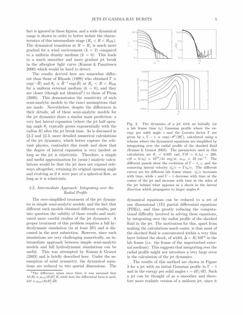
Fig. 3. The dynamics of a jet with an initially (ata lab frame time t0) Gaussian profile where the en-ergy per solid angle ǫ and the Lorentz factor Γ aregiven by ǫ, Γ − 1 ∝ exp(−θ2/2θ2

c ), calculated using ascheme where the dynamical equations are simplified byintegrating over the radial profile of the shocked fluid(Kumar & Granot 2003). The parameters used in thiscalculation are θc = 0.035 rad, Γ(θ = 0, t0) = 200,ǫ(θ = 0, t0) = 1053/4π erg/sr, next = 10 cm−3. Thedifferent panels show the evolution of Γ − 1, ǫ, and thecomoving lateral velocity v′

θ/c = Γvθ/c. The differentcurves are for different lab frame times: v′

θ/c increaseswith time, while ǫ and Γ − 1 decrease with time at thecenter of the jet and increase with time at the sides ofthe jet behind what appears as a shock in the lateraldirection which propagates to larger angles θ.

dynamical equations can be reduced to a set ofone dimensional (1D) partial differential equations(PDEs), and thus greatly reducing the computa-tional difficulty involved in solving these equations,by integrating over the radial profile of the shockedfluid in the jet. The motivation for this, apart frommaking the calculations much easier, is that most ofthe shocked fluid is concentrated within a very thinlayer behind the shock, of width ∆ ∼ R/10Γ2 in thelab frame (i.e. the frame of the unperturbed exter-nal medium). This suggests that integrating over theradial profile might not introduce a very large errorin the calculation of the jet dynamics.

The results of this method are shown in Figure3 for a jet with an initial Gaussian profile in Γ − 1and in the energy per solid angles ǫ = dE/dΩ. Sucha jet can be thought of as a smoother and there-fore more realistic version of a uniform jet, since it

6 GRANOT

Fig. 4. The dynamics of a “structured” jet where initiallyΓ−1 = 200/(1+θ2/θ2

c ) and ǫ = ǫ0/(1−θ2/θ2c ) with ǫ0 =

1053/4π erg/sr, θc = 0.02 rad, and next = 10 cm−3. Theformat is similar to Figure 3. Again v′

θ/c increases withtime while Γ−1 decreases with time. For a structured jet,as opposed to an initially Gaussian jet, a shock does notdevelop in the lateral direction and ǫ(θ) remains almostunchanged as long as the jet is relativistic.

has a roughly uniform core and relatively sharp (butstill smooth) wings. A shock appears to develop inthe lateral direction, because of the very steep initialangular profile in the wings of the Gaussian. Never-theless, the lateral expansion remains modest as longas the jet is relativistic. This can be seen both fromthe small (compared to c) lateral velocity in the co-moving frame, and from the fact that ǫ(θ) does notchange very much compared to its initial distribu-tion. The modest degree of lateral spreading is instark contrast with the results of semi-analytic mod-els.

Figure 4 shows the resulting dynamics for a“structured” jet (which is discussed in §3) whereΓ and ǫ are initially power laws with the angle θfrom the jet symmetry axis, outside of some narrowcore. Again, there is very little lateral expansion (i.e.the comoving lateral velocity remains ≪ c and ǫ(θ)hardly deviates from its initial profile) as long as thejet core is relativistic.

2.3. Hydrodynamic Simulations

The most reliable method for calculating the jetdynamics is using hydrodynamic simulations. Thisis a formidable numerical task for the following rea-sons. First, it requires a hydrodynamic code with

Fig. 5. A 3D view of a relativistic impulsive jet at thelast time step of the simulation (Granot et al. 2001). Theouter surface represents the shock front while the two in-ner faces show the proper number density (lower face)and proper synchrotron emissivity (upper face) in a log-arithmic color scale.

special relativity that is accurate over a large rangein the four velocity u = Γβ, from u ≈ Γ ≫ 1 tou ≈ β ≪ 1. Second, the shocked fluid in the jet isconcentrated in a very thin layer behind the shock,of width ∆ ∼ R/10Γ2 in the lab frame, which isextremely narrow at early times when Γ ≫ 1, andtherefore very hard to resolve properly.

More specifically, from considerations of causal-ity, significant lateral expansion could in princi-pal occur when Γ becomes comparable to θ−1

0 , sothat ideally one would want to start with an ini-tial Lorentz factor Γ0 ≫ θ−1

0 , and in practicewe need at least Γ0θ0 ∼

> a few. Observed jetbreak times suggest 0.05 ∼

< θ0 ∼< 0.2 and there-

fore require Γ0 ∼> 20 − 100. If 100N2 cells are

needed in order to resolve the shell of width ∆ ∼R/10Γ2 then the minimal cell size in the initialtime step (denoted by the subscript ‘0’) needs tobe of the order of δ ∼ 10−6N−1

2 (Γ0/30)−2R0 ∼10−6N−1

2 (Γ0θ0/3)−2(θ0/0.1)2R0. The minimal num-ber of cells required to resolve the initial shell isNmin ∼ θ0R0∆0δ

−2 ∼ 107N22 (Γ0θ0/3)2(θ0/0.1)−1.

The total number of cells in each time step can beNtot ∼ Nmin if the code uses adaptive mesh re-finement (AMR). Otherwise, for a fixed cell size,Ntot/Nmin ∼

> R0/∆0 ∼ 104(Γ0θ0/3)2(θ0/0.1)−2.

Because of the numerical difficulty involved, veryfew attempts have been made so far (Granot et al.2001; Cannizzo et al. 2004). In the following I shall

JETS IN GAMMA-RAY BURSTS 7

100 150 200 250 300 350 400

2

4

6

8

10

12

weighed by number density

weighed by emissivity

maximal values

R=ct

tdays

R /

1017

cm

80 90 100 200 300 400

10−1

100

101

tdays

Γ −

1

weighed by number density

weighed by emissivity

maximal values

100 150 200 250 300 350 4000

0.1

0.2

0.3

0.4

0.5

0.6

0.7

0.8

0.9

θ0

2θ0

weighed by number density

weighed by emissivity

maximal values

tdays

θ

Fig. 6. The jet radius (upper panel), Lorentz factor minusone (middle panel), and angle θ from the jet symmetryaxis (lower panel), as a function of the lab frame timetlab ≈ R/c (in days), from a hydrodynamic simulation(Granot et al. 2001).

concentrate on the results of Granot et al. (2001).6

The initial conditions were a cone of half-openingangle θ0 = 0.2 rad, taken out of the spherical

6The calculations of Cannizzo et al. (2004) suffer frompoor numerical resolution.

Blandford & McKee (1976) self-similar solution withan (isotropic equivalent) energy of Ek,iso = 1052 ergand a uniform external density of next = 1 cm−3.The initial Lorentz factor of the fluid just behind theshock was Γ0 ≈ 16.8 corresponding to Γ0θ0 ≈ 3.4.

The results of the simulation are illustrated inFigures 5 and 6. While the number density doesnot change significantly between the front and thesides of the jet, the emissivity is large only at thefront of the jet, within its initial half-opening angle(θ < θ0), and drops sharply at θ > θ0. This causesthe emissivity weighted values of the Lorentz factorand radius to be close to their maximal values (whichare also obtained at the front of the jet). Whilethe sides of the jet contribute a small fraction ofthe total emissivity, their emission can dominate theobserved flux for lines of sight outside the initial half-opening angle of the jet, as discussed in §3.5. Theoverall egg-shaped structure of the shock front is verydifferent from the quasi-spherical structure assumedin 1D semi-analytic models. Moreover, the degreeof lateral expansion is very modest as long as thehead of the jet is relativistic, in contradiction withthe very rapid lateral expansion predicted by semi-analytic models.

2.4. The Afterglow Emission

The dominant emission mechanism during the af-terglow stage is believed to be synchrotron emission.This is supported by the detection of linear polar-ization at the level of ∼ 1% − 3% in several opti-cal or NIR afterglows (see §3.3), and by the shapeof the broad band spectrum, which consists of sev-eral power-law segments that smoothly join at sometypical break frequencies. Synchrotron self-Compton(SSC; the inverse-Compton scattering of the syn-chrotron photons by the same population of relativis-tic electrons that emits the synchrotron photons) cansometimes dominate the afterglow flux in the X-rays(Sari & Esin 2001; Harrison et al. 2001).

It is usually assumed that the electrons are(practically instantaneously) shock-accelerated intoa power law distribution of energies, dN/dγe ∝ γ−p

e

for γe > γm, and thereafter cool both adiabaticallyand due to radiative losses. Furthermore, it is as-sumed that practically all of the electrons take partin this acceleration process and form such a non-thermal (power-law) distribution, leaving no ther-mal component (which is not at all clear or justi-fied; e.g. Eichler & Waxman 2005). The relativisticelectrons are assumed to hold a fraction ǫe of the in-ternal energy immediately behind the shock, whilethe magnetic field is assumed to hold a fraction ǫB

8 GRANOT

ν2

t1t1/2 ν1/3

t0t1/2

ν(1−p)/2

t(1−

3p)/

4

t3(1−

p)/4

ν−p/2

t(2−

3p)/

4

t(2−

3p)/

4

νsa

(1)

t0

t−3/5 νm

(2)

t−3/2

t−3/2ν

c

(3) t−1/2

t1/2B D G H

ISM scalingsWIND scalings

ISM

sca

lings

WIN

D s

calin

gs spectrum 1

ν2

t1t1/2 ν5/2

t7/4

t5/4

ν(1−p)/2

t(1−

3p)/

4

t3(1−

p)/4

ν−p/2

t(2−

3p)/

4

t(2−

3p)/

4

νm

(4)t−3/2

t−3/2 νsa

(5)

t−(3p+2)/2(p+4)

t−3(p+2)/2(p+4)

νc

(3)

t−1/2

t1/2

B A G H

spectrum 2

ν2

t1t1/2 ν5/2

t7/4

t5/4

ν−p/2

t(2−

3p)/

4

t(2−

3p)/

4

νm

(4)t−3/2

t−3/2 νsa

(6)

t−3(p+1)/2(p+5)

t−(3p+5)/2(p+5)

B A H

Log(

Fν)

spectrum 3

ν2

t1t1/2 ν11/8

t1

t11/1

6

ν−1/2

t−1/

4

t−1/

4

ν−p/2

t(2−

3p)/

4

t(2−

3p)/

4

νac

(7) t3/10

t0 νsa

(8)

t−1/2

t−2/3

νm

(9)

t−3/2

t−3/2

B C F H

spectrum 4

108

1010

1012

1014

1016

1018

ν2

t1t1/2 ν11/8

t1

t11/1

6

ν1/3 t−2/

3

t1/6

ν−1/2

t−1/

4

t−1/

4

ν−p/2

t(2−

3p)/

4

t(2−

3p)/

4

νac

(7)

t3/10

t0ν

sa

(10)

t−1/2

t−8/5ν

c

(11)

t−1/2

t1/2 νm

(9)

t−3/2

t−3/2

B C E F H

ν in Hz

spectrum 5

Fig. 7. The afterglow synchrotron spectrum, calculatedfor the Blandford & McKee (1976) spherical self-similarsolution, under standard assumptions, using the accurateform of the synchrotron spectral emissivity and integra-tion over the emission from the whole volume of shockedmaterial behind the forward (afterglow) shock (for de-tails see Granot & Sari 2002). The different panels showthe five possible broad band spectra of the afterglow syn-chrotron emission, each corresponding to a different or-dering of the spectral break frequencies. Each spectrumconsists of several power law segments (PLSs; each shownwith a different color and labeled by a different letterA–H) that smoothly join at the break frequencies (num-bered 1–11). The broken power law spectrum, whichconsists of the asymptotic PLSs that abruptly join atthe break frequencies (and is widely used in the litera-ture), is shown for comparison. Most PLSs appear inmore than one of the five different broad band spectra.Indicated next to the arrows are the temporal scaling ofthe break frequencies and the flux density at the differ-ent PLSs, for a uniform (ISM) and stellar wind (WIND)external density profile.

of the internal energy everywhere in the shocked re-gion. This is a convenient parameterization of ourignorance regarding the micro-physics of relativisticcollisionless shocks, which are still not sufficiently

well understood from first principals.The spectral emissivity in the co-moving frame

of the emitting shocked material is typically approxi-mated as a broken power-law (in some cases the moreaccurate functional form of the synchrotron emissionis used, e.g. Wijers & Galama 1999; Granot & Sari2002). Most calculations of the light curve assumeemission from an infinitely thin shell, which repre-sents the shock front (some integrate over the volumeof the shocked fluid taking into account the appro-priate radial profile of the flow, e.g. Granot & Sari2002, see Figure 7). One also needs to account forthe different arrival times of photons to the observerfrom emission at different lab frame times and loca-tions relative to the line of sight, as well as the rel-evant Lorentz transformations of the emission intothe observer frame. SSC is included in some (notall) works, although it can also effect the synchrotronemission through the enhanced radiative cooling ofthe electrons.

2.5. The afterglow Image

The apparent surface brightness distribution andsize evolution of the afterglow image on the planeof the sky can potentially provide very useful infor-mation about the structure and dynamics of GRBjets, as well as about the radial dependence of theexternal density. Furthermore, polarimetry (or evenspectral polarimetry) of a resolved afterglow imagecould provide valuable information on the magneticfield structure behind collisionless relativistic shocks,which is not well understood theoretically. However,most GRBs are at cosmological distances (z ∼

> 1)and the angular size of their afterglow image is ofthe order of a micro-arcsecond (µas) after a day orso, making it extremely difficult to resolve the image.

During the self-similar spherical evolution stage(before the jet break time, for a jet), the afterglowimage has circular symmetry around the line of sight(where the surface brightness depends only on thedistance from the center of the image), and is con-fined within a circle on the sky with a radius

R⊥

1016 cm=

3.91(

E52

n0

)1/8 (

tdays

1+z

)5/8

(k = 0)

2.39(

E52

A∗

)1/4 (

tdays

1+z

)3/4

(k = 2)

.

(15)(see Figure 8) where E52 is the isotropic equivalentafterglow kinetic energy in units of 1052 erg, tdays

is the observed time in days, and the external den-sity is assumed to be a power law with the distanceR from the central source, ρext = nextmp = AR−k,where n0 = next/(1 cm−3) for a uniform external

JETS IN GAMMA-RAY BURSTS 9

Fig. 8. Schematic illustration of the equal arrival timesurface (thick black line), namely, the surface from wherethe photons emitted at the shock front arrive at the sametime to the observer (on the far right-hand side). Themaximal lateral extent of the observed image, R⊥, is lo-cated at an angle , where the shock radius and Lorentzfactor are R∗ and Γ∗ = Γsh(R∗), respectively. The areaof the image on the plane of the sky is S⊥ = πR2

⊥. Theshock Lorentz factor, Γsh, varies with radius R and angleθ from the line of sight along the equal arrival time sur-face. The maximal radius Rl on the equal arrival timesurface is located along the line of sight. If, as expected,Γsh decreases with R, then Γl = Γsh(Rl) is the minimalshock Lorentz factor on the equal arrival time surface.(from Granot, Ramirez-Ruiz & Loeb 2005).

density (k = 0), and A∗ = A/(5 × 1011 g cm−1) fora wind-like external density profile (k = 2) as mightbe expected for a massive star progenitor. This cor-responds to an angular radius of

R⊥

dA=

1.61 µasdA,27.7

(

E52

n0

)1/8 (

tdays

1+z

)5/8

(k = 0)

0.98 µasdA,27.7

(

E52

A∗

)1/4 (

tdays

1+z

)3/4

(k = 2)

.

(16)where dA(z) is the angular distance to the source,and dA,27.7 is dA in units of 1027.7 cm ≈ 5×1027 cm. 7

More generally, the afterglow image size duringthe self-similar spherical stage scales with the ob-served time as R⊥ ∝ t(5−k)/2(4−k). The image sizegrows super-luminally with an apparent expansionvelocity of Γsh(R∗)c. The expected afterglow imagesin this self-similar regime are shown in Figures 9 and10. The normalized surface brightness profile withinthe afterglow image is independent of time due tothe self-similar dynamics, and changes only betweenthe different power law segments of the synchrotronspectrum, and for different external density profiles.The image becomes increasingly limb-brightened athigher frequencies, and for smaller values of k.

Below the self-absorption frequency the spe-

7For a standard cosmology (ΩM = 0.27, ΩΛ = 0.73, h =0.72) dA(z) has a maximum value of 5.37×1027 cm (dA,27.7 =1.07) for z = 1.64.

0

0.5

1

1.5

2

2.5

3

β = −p/2

β = (1−p)/2

β = 1/3

β = 2

β = 5/2

k = 0

0 0.2 0.4 0.6 0.8 10

0.5

1

1.5

2

2.5

3

r

Iν

/ <

I ν >

β = −p/2

β = (1−p)/2

β = 1/3

β = 2

β = 5/2

k = 2

Fig. 9. The afterglow images for different power law seg-ments of the spectrum, for a uniform (k = 0) and wind(k = 2) external density profile (from Granot & Loeb2001, calculated for the Blandford & McKee 1976 spher-ical self similar solution, using the formalism ofGranot & Sari 2002). Shown is the surface brightness,normalized by its average value, as a function of thenormalized distance from the center of the image, r =R sin θ/R⊥ (where r = 0 at the center and r = 1 at theouter edge). The image profile changes considerably be-tween different power-law segments of the afterglow spec-trum, Fν ∝ νβ. There is also a strong dependence on thedensity profile of the external medium, ρext ∝ R−k.

cific intensity (surface brightness) represents theRayleigh-Jeans portion of a black-body spectrumwith the blue-shifted effective temperature of theelectrons at the corresponding radius along the frontside of the equal arrival time surface of photons tothe observer (R∗ ≤ R ≤ Rl in Figure 8). Abovethe cooling break frequency the emission originatesfrom a very thin layer behind the shock front wherethe electrons whose typical synchrotron frequency isclose to the observed frequency have not yet hadenough time to significantly cool due to radiativelosses. This results in a divergence of the surface

10 GRANOT

ν << νa νa << ν << νm νm << ν << νc

Fig. 10. An illustration of the expected afterglow imageon the plain of the sky, for three different power lawsegments of the spectrum (from Granot, Piran & Sari1999a,b), assuming a uniform external density and theBlandford & McKee (1976) self-similar solution. The im-age is more limb brightened at power law segments thatcorrespond to higher frequencies.

brightness at the outer edge of the image (Sari 1998;Granot & Loeb 2001).

After the jet break time the afterglow image isno longer symmetric around the line of sight to thecentral source for a general viewing angle (which isnot exactly along the jet symmetry axis), and itsdetails depend on the the hydrodynamic evolutionof the jet (so that in principal it could be used inorder to constrain the jet dynamics). Therefore, arealistic calculation of the afterglow image during themore complicated post-jet break stage requires theuse of hydrodynamic simulation, and still remains tobe done.

The afterglow image may be indirectly resolvedthrough gravitational lensing by a star in an inter-vening galaxy (along, or close to, our line of sightto the source). This is since the angular size of theEinstein radius (i.e. the region of large magnifica-tion around the lensing star) for a typical star at acosmological distance is ∼ 1 µas (hence the namemicro-lensing), and therefore comparable to the af-terglow image size after a day or so. Since the af-terglow image size grows very rapidly with time, dif-ferent parts of the image sample the regions of largemagnification (close to the point of infinite magnifi-cation just behind the lensing star) with time, andtherefore the overall magnification of the afterglowflux as a function of time probes the surface bright-ness profile of the afterglow image. This results in abump in the afterglow light curve which peaks whenthe limb-brightened outer part of the image sweepspast the lensing star, where the peak of the bumpis sharper the more limb-brightened the afterglowimage (Granot & Loeb 2001). It has been suggestedthat an achromatic bump in the afterglow light curveof GRB 000301C after ∼ 4 days might have been dueto micro-lensing (Garnavich, Loeb & Stanek 2000).

10−2

10−1

100

101

102

103

104

1016

1017

1018

1019

t (in days)

2R⊥ (i

n cm

)

model 1; E51/n0=0.8; θ0=0.12

model 2; E51/n0=5; θ0=0.09

ISM (k=0)

model 2; E51/A*=1.2; θ0=0.32

model 1; E51/A*=2; θ0=0.25

wind (k=2)

Fig. 11. Tentative fits to the constraints on the image size(or diameter 2R⊥) of the radio afterglow of GRB 030329at different epochs, for different external density profilesand different assumptions on the lateral spreading of thejet. The physical parameters and external density pro-file for each model are indicated (the viewing angle isalong the jet symmetry axis). Model 1 features relativis-tic sideways expansion in the co-moving rest frame ofthe jet material, while model 2 has no lateral spreading(from Granot, Ramirez-Ruiz & Loeb 2005).

If this interpretation is true, then the shape of thebump in the afterglow light curve requires a limb-brightened afterglow image, in agreement with the-oretical expectations (Gaudi, Granot & Loeb 2001).

The size of the afterglow image at a sin-gle epoch can be estimated from the quenchingof diffractive scintillations in the radio afterglow(Goodman 1997; Frail et al. 1997; Taylor et al. 1997;Waxman, Kulkarni & Frail 1998). The flux be-low the self-absorption frequency can also be usedto constrain the size of the emitting region (e.g.,Katz & Piran 1997; Granot, Ramirez-Ruiz & Loeb2005). A more direct measurement of the imagesize, as well as its temporal evolution, may be ob-tained through very large base-line interferometry inthe radio (i.e. with the VLBA). This was possiblefor only for one radio afterglow so far (GRB 030329;Taylor et al. 2004, 2005), since it requires a rela-tively nearby event (z ∼

< 0.2) with a bright ra-dio afterglow. Nevertheless, it already providesinteresting constraints (Oren, Nakar & Piran 2004;Granot, Ramirez-Ruiz & Loeb 2005, see Figure 11),and better observations in the future may help pindown the jet structure and dynamics, as well as theexternal density profile.

JETS IN GAMMA-RAY BURSTS 11

2.6. What causes the Jet Break?

The jet break in the afterglow light curve hasbeen argued to be the combination of (i) the edge ofthe jet becoming visible, and (ii) fast lateral spread-ing. Both effects are expected to take place aroundthe same time, when the Lorentz factor, Γ, of thejet drops below the inverse of its initial half-openingangle, θ0. This can be understood as follows.

When Γ drops below θ−10 the edge of the jet be-

comes visible, since relativistic beaming limits theregion from which a significant fraction of the emit-ted radiation reaches the observer to within an angleof ∼ Γ−1 around the line of sight (θ ∼

< Γ−1). Oncethe edge of the jet becomes visible, then if there isno significant lateral spreading, only a small fraction(Γθj)

2 < 1 of the visible region is occupied by thejet, and therefore there would be “missing” contri-butions to the observed flux compared to a spheri-cal flow. This would cause a steepening in the lightcurve, i.e. a jet break, where the temporal decay in-dex asymptotically increases by ∆α = (3−k)/(4−k).

When Γ drops below θ−10 , the center of the jet

comes into causal contact with its edge, and thejet can in principal start to expand sideways sig-nificantly. It has been argued that at this stage itwould indeed start to expand sideways rapidly, atclose to the speed of light in its own rest frame. Inthis case, during the rapid lateral expansion phasethe jet opening angle grows as θj ∼ Γ−1 and ex-ponentially with radius (see §2.1). This causes theenergy per solid angle, ǫ, in the jet to drop withobserved time, and the Lorentz factor to decreasefaster as a function of the observed time, which re-sult a steepening in the afterglow light curve com-pared to a spherical flow (where ǫ remains constantand Γ decreases more slowly with the observed time).However, in this case a good part of the visible re-gion remains occupied by the jet (since Γθj remains∼ 1), so that the first cause for the jet break (theedge of the jet becoming visible, and the “missing”contributions from outside the edge of the jet) is nolonger important. Therefore, for fast lateral spread-ing, the jet break is caused predominantly since theenergy per solid angle ǫ decreases with time, and theLorentz factor decreases with observed time fasterthan for a spherical flow.

It is important to keep in mind, however, thatnumerical studies show that the lateral spreading ofthe jet is very modest as long as it is relativistic (see§2.2 and §2.3). This implies that lateral spreadingcannot play an important role in the jet break, andthe predominant cause of the jet break is the “miss-ing” contribution from outside of the jet, once its

10−2

10−1

100

101

102

1

1.25

1.5

1.75

2

2.25

2.5

tobs (days)

α =

− d

log(

Fν) /

dlo

g(t)

ISM

wind

Shape of the Jet Break

p = 2.5, ν > max(νm,νc)

10−1

100

101

102

0.5

1

1.5

2

2.5

3

tobs (days)

α =

− d

log(

Fν) /

dlo

g(t)

semi−analytic model

with no lateral expansion

hydrodynamic

simulation

Shape of the Jet Break

p = 2.5 , νm < ν < νc

Fig. 12. The temporal decay index α as a function of theobserved time (in days) across the jet break in the lightcurve, for p = 2.5. Upper panel: results in the spectralrange ν > max(νm, νc) using a semi-analytic model withno lateral spreading (Granot 2005), for a uniform (k = 0,next = 1 cm−3) and wind (k = 2, A∗ = 1) external den-sity profile, with θ0 = 0.1 and Ek,iso = 2 × 1053 erg.Lower panel: results for the spectral range νm < ν < νc,for θ0 = 0.2 and a uniform density (k = 0, next = 1 cm−3,Ek,iso = 1052 erg); compares the result of a semi-analyticmodel (Granot 2005) to those of a hydrodynamic simu-lation (Granot et al. 2001). In both panels the dashedlines show the asymptotic values of α before and afterthe jet break, for a uniform jet with no lateral spreading,for which ∆α = (3 − k)/(4 − k).

edge becomes visible.

A potential problem with this picture is that ifthe jet half-opening angle remains roughly constant,θj ≈ θ0, the asymptotic change in the temporal de-cay index is only ∆α = 3/4 for a uniform exter-nal medium (k = 0) or even smaller for a wind(∆α = 1/2 for k = 2), while the values inferred

12 GRANOT

from observations are in most cases larger (see Fig-ure 3 of Zeh, Klose & Kann 2006). This apparentdiscrepancy may be reconciled as follows. While theasymptotic steepening is indeed ∆α = (3−k)/(4−k)when lateral expansion is negligible, the value of thetemporal decay index α (where Fν ∝ t−α) initiallyovershoots its asymptotic value. Since the temporalbaseline that is used in order to measure the post-jetbreak temporal decay index α2 is typically no morethan a factor of several in time after the jet breaktime8, tjet, the value of α during this time is largerthan its asymptotic value α2. This causes the valueof ∆α that is inferred from observations to be largerthan its asymptotic value.

The overshoot in the value of α just after thejet break time can nicely be seen in Figure 12, andis much more pronounced in the light curves calcu-lated using the jet dynamics from a hydrodynamicsimulation, compared to the results of a simple semi-analytic model. The cause of this overshoot is thatthe afterglow image is limb-brightened (see Figure9) and therefore the outer edges of the image whichare the brightest are the first region whose contri-bution to the observed flux is “missed” as the edgeof the jet becomes visible. The overshoot is largerthe more limb-brightened the afterglow image (e.g.,for ν > max(νm, νc) in the upper panel of Figure12 compared to νm < ν < νc in the lower panel ofFigure 12). For a wind density (k = 2) the limb-brightening is smaller compared to a uniform den-sity (k = 0), at the same power law segment of thespectrum (see Figure 9), and the Lorentz factor Γdecreases more slowly with the observed time. Be-cause of this no overshoot is seen in the semi-analyticmodel shown in the upper panel of Figure 12 for awind density profile (k = 2), and the jet break issmoother and extends over a larger factor in time.The asymptotic post-jet break value of the temporaldecay index (α2) is approached only when the visi-ble part of the afterglow image covers the relativelyuniform central part, and not its brighter outer edge.

The jet break in light curves calculated fromhydrodynamic simulations is sharper than in semi-analytic models (where the emission is taken to befrom a 2D surface – usually a section of a spherewithin a cone). In semi-analytic models the jet breakis sharpest with no lateral expansion, and becomesmore gradual the faster the assumed lateral expan-sion. For example, in the lower panel of Figure 12,where the viewing angle is along the jet axis and the

8This is usually because the flux becomes too dim to de-tect above the host galaxy, or since a supernova componentbecomes dominant in the optical, etc.

external density is uniform, most of the change inthe temporal decay index α occurs over a factor of∼ 2 in time for the numerical simulation, and overa factor of ∼ 3 in time for the semi-analytic model(which assumes no lateral expansion; the jet breakwould be more gradual with lateral expansion). Forboth types of models, the jet break is more grad-ual and occurs at a somewhat later time for viewingangles further away from the jet symmetry axis butstill within its initial opening angle, although this ef-fect is somewhat more pronounced in semi-analyticmodels (Granot et al. 2001; Rossi et al. 2004).

3. THE JET STRUCTURE

Since the initial discovery of GRB after-glows in the X-ray (Costa et al. 1997), optical(van Paradijs et al. 1997), and radio (Frail et al.1997), many afterglows have been detected and thequality of individual afterglow light curves has im-proved dramatically (e.g., Lipkin et al. 2004). De-spite all the observational and theoretical progress,the structure of GRB jets remains largely an openquestion. This question is of great importance andinterest, since it is related to issues that are funda-mental for our understanding of GRBs, such as theirevent rate, total energy, and the requirements fromthe compact source that accelerates and collimatesthese jets.

In §3.1 a brief overview is given of the main jetstructures that have been discussed in the literatureand the motivation for them. This is followed by adiscussion of the different methods that have beenapplied for constraining the jet structure from ob-servations, which include statistical studies (§3.2), aswell as the evolution of the linear polarization of theafterglow emission (§3.3), and the shape of the after-glow light curves (§3.4). The afterglow light curvesfrom viewing angles outside the initial jet apertureare discussed in §3.5 along with possible implicationsfor X-ray flashes and for the jet structure, while §3.6briefly mentions the search for orphan afterglows.Some implications of recent Swift observations arediscussed in §3.7.

3.1. Existing Models for the Jet Structure

The leading models for the jet structureare (i) the uniform jet (UJ) model (Rhoads1997, 1999; Panaitescu & Meszaros 1999;Sari, Piran & Halpern 1999; Kumar & Panaitescu2000; Moderski, Sikora & Bulik 2000; Granot et al.2001, 2002), where the energy per solid angle, ǫ, andthe initial Lorentz factor, Γ0, are uniform withinsome finite half-opening angle, θj , and sharply drop

JETS IN GAMMA-RAY BURSTS 13

outside of θj ; and (ii) the universal structured jet(USJ) model (Lipunov, Postnov & Prokhorov 2001;Rossi et al. 2002; Zhang & Meszaros 2002), whereǫ and Γ0 vary smoothly with the angle θ from thejet symmetry axis. In the UJ model the differentvalues of the jet break time, tj , in the afterglowlight curve arise mainly due to different θj (and toa lesser extent due to different ambient densities).In the USJ model, all GRB jets are intrinsicallyidentical, and the different values of tj arise mainlydue to different viewing angles, θobs, from the jetaxis.9

The observed correlation, tj ∝ E−1γ,iso (Frail et al.

2001; Bloom, Frail & Kulkarni 2003), implies aroughly constant true energy, E, between differ-ent GRB jets in the UJ model, and ǫ ∝ θ−2 out-side of some core angle, θc, in the USJ model(Rossi et al. 2002; Zhang & Meszaros 2002). Thisis assuming a constant efficiency, ǫγ , for producingthe observed prompt gamma-ray (or X-ray) emis-sion. If the efficiency depends on θ in the USJmodel, for example, then different power laws ofǫ with θ are possible (Guetta, Granot & Begelman2005), such as a core with wings where ǫ ∝θ−3, as is obtained in simulations of the col-lapsar model (Zhang, Woosley & MacFadyen 2003;Zhang, Woosley & Heger 2004).10

The jet structure was initially envisioned to beuniform since this is the simplest jet structure, andarguably also the most natural. Furthermore, italso predicted a jet break in the afterglow lightcurve (Rhoads 1997, 1999; Sari, Piran & Halpern1999), which was soon thereafter confirmed observa-tionally (Fruchter et al. 1999; Kulkarni et al. 1999a;Stanek et al. 1999). The original motivation for theUSJ model was the conceptual simplicity of a uni-versal intrinsic structure for all GRB jets, where theobserved differences (namely in the jet break times)arise due to different viewing angles (instead of beingattributed to an intrinsic difference - in the jet half-opening angle - as in the UJ model). Its exact struc-ture was motivated by the requirement to reproducethe observed afterglow light curves and correlationswith the prompt GRB emission. It had later beensuggested on theoretical grounds that a jet struc-ture with a narrow core and wings where ǫ ∝ θ−2 is

9In fact, the expression for tj is similar to that for a uniformjet with ǫ → ǫ(θ = θobs) and θj → θobs

10Simulations of jets launched by an accretion torus - blackhole system, where the jet does not propagate through astellar envelope, as is expected to arise in binary mergerscenarios which might be relevant to GRBs of the short-hard class, produce a roughly uniform jet with sharp edges(Aloy, Janka & Kuller 2005).

0.2 0.4 0.6 0.8 1 1.2 1.4

0.5

1

1.5

2

2.5

3

3.5

4

4.5x 10

53

θ

dE /

dΩ (

erg

/ 4π

sr)

10−3

10−2

10−1

100

1048

1049

1050

1051

1052

1053

1054

θ

dE /

dΩ (

erg

/ 4π

sr)

universal structured jet

uniform ("top hat") jet

Gaussian jet

2 component jet

"ring" shaped jet

"fan" shaped jet

Fig. 13. An illustration of various jet structures that havebeen discussed in the literature, in terms of the distribu-tion of their energy per solid angle, ǫ = dE/dΩ, withthe angle θ from the jet symmetry axis, both in semi-logarithmic scale (main figure) and in log-log scale (biginset). Both the normalization of dE/dΩ and the typicalangular scale may vary in most models, and their val-ues shown here were chosen to be more or less “typical”.(from Granot 2005).

expected in highly magnetized Poynting flux domi-nated jets (Lyutikov & Blandford 2002, 2003) as wellas in low magnetization hydrodynamic jets in thecontext of the collapsar model (Lazzati & Begelman2005; see, however, Morsony, Lazzati & Begelman2006).

Other jet structures have also been proposed inthe literature. Figure 13 illustrates different jetstructures that have been discussed in the litera-ture in terms of their distribution of ǫ(θ). A jetwith a Gaussian angular profile (Zhang & Meszaros2002; Kumar & Granot 2003) may be thought of asa more realistic version of a uniform jet, where theedges are smooth rather than sharp. A Gaussianǫ(θ) ∝ exp(−θ2/2θ2

c) is approximately intermediatebetween the UJ and USJ models, but it is closer tothe UJ model than to the USJ model with ǫ ∝ θ−2

in the sense that for a Gaussian ǫ(θ) the energy inthe wings of the jet is much smaller than in its core,whereas for a USJ with ǫ ∝ θ−2 wings there is equalenergy per decade in the wings, and therefore thewings contain more energy than the core (by aboutan order of magnitude).

Another jet structure that received some at-tention recently is a two-component jet model(Pedersen et al. 1998; Frail et al. 2000; Berger et al.2003b; Huang et al. 2004; Peng, Konigl & Granot2005; Wu et al. 2005) with a narrow uniform jetof initial Lorentz factor Γ0 ∼

> 100 surrounded by a

14 GRANOT

wider uniform jet with Γ0 ∼ 10 − 30. Theoreticalmotivation for such a jet structure has been foundboth in the context of the cocoon in the collapsarmodel (Ramirez-Ruiz, Celotti & Rees 2002) and inthe context of a hydromagnetically driven neutron-rich jet (Vlahakis, Peng & Konigl 2003). This modelhas been invoked in order to account for sharpbumps (i.e., fast rebrightening episodes) in the af-terglow light curves of GRB 030329 (Berger et al.2003b) and XRF 030723 (Huang et al. 2004). Adifferent motivation for proposing this jet structureis in order to account for the energetics of GRBsand X-ray flashes and reduce the high efficiency re-quirements from the prompt gamma-ray emission(Peng, Konigl & Granot 2005).

More “exotic” jet structures have also been con-sidered. One example is a jet with a cross sec-tion in the shape of a “ring,” sometimes referred toas a “hollow cone” (Levinson & Eichler 1993, 2000;Eichler & Levinson 2003, 2004; Lazzati & Begelman2005), which is uniform within θc < θ < θc + ∆θwhere ∆θ ≪ θc. Another example is a “fan”-or “sheet”-shaped jet (Thompson 2005) where amagnetocentrifugally launched wind from the proto-neutron star, formed during the supernova explosionin the massive star progenitor, becomes relativisticas the density in its immediate vicinity drops and isenvisioned to form a thin sheath of relativistic out-flow that is somehow able to penetrate through theprogenitor star along the rotational equator, forminga relativistic outflow within ∆θ ≪ 1 around θ = π/2(or θc = π/2 − ∆θ/2).11

3.2. Statistical Studies

One approach for constraining the jet structureis through statistical studies of the prompt emis-sion. In particular, a convenient observable is thelog N − log S distribution, where N is the number ofGRBs observed above a limiting peak photon fluxS (Firmani et al. 2004; Guetta, Piran & Waxman2005; Guetta, Granot & Begelman 2005; Xu et al.2005). In this type of study one needs to assumeboth the intrinsic GRB event rate (which is usuallyassumed to follow the star formation rate), and theluminosity function which depends on the jet struc-ture through the isotropic equivalent luminosity L(θ)as a function of the angle θ from the jet symmetryaxis. The latter depends in turn on the angular dis-tribution of the energy per solid angle in the jet ǫ(θ)

11This has been suggested as a possible jet structure withinthis model, but the final jet structure is by no means clear,and other jet structures might also be possible within thismodel (T. A. Thompson 2005, private communication).

Fig. 14. The probability distribution, dN/dzd ln θ, ofthe observed GRB rate as a function of redshift z andviewing angle θ, as predicted by the USJ model (fromNakar, Granot & Guetta 2004). The white contour linesconfine the minimal area that contains 1 σ of the totalprobability. The circles denote the 16 GRBs with knownz and θ from the sample of Bloom, Frail & Kulkarni(2003). (a) The model parameters are similar to thoseof Perna, Sari & Frail (2003). This figure is the 2D re-alization of their Figure 1. (b) Here a limited range inredshift is used, 0.8 < z < 1.7 (containing 10 out of the16 data points), in order to minimize redshift selectioneffects and reduce the sensitivity of the results to theunknown GRB rate. Measurement errors of 20% in ln θ(σln θ = 0.2) were included and a log-normal distributionin the effective duration that they deduced from obser-vations.

and the gamma-ray efficiency ǫγ(θ), whose product(times 4π) provides the isotropic equivalent energyoutput in gamma-rays, Eγ,iso(θ), and the assumeddistribution of the peak isotropic equivalent lumi-nosity for a given Eγ,iso.

For the USJ model ǫ(θ) and ǫγ(θ) are assumedto be power laws in θ and one needs to specify theirpower law indexes, as well as the jet core angle θc

and outer edge θmax (Guetta, Granot & Begelman2005). For the UJ model one needs to specifythe distribution of jet half-opening angles θ0, whichcan be taken to be a power law distribution inthe range θmin < θ0 < θmax. These simple formsof the USJ and UJ models are degenerate, sincethey both produce a power law luminosity function

JETS IN GAMMA-RAY BURSTS 15

(Guetta, Granot & Begelman 2005), which providesan adequate fit to the data. The total rate of en-ergy release in gamma-rays must be the same inboth models (and match the observed rate), wherein the USJ model it is released in fewer more ener-getic events (by a factor of ∼ 10; see equation 14 ofGuetta, Granot & Begelman 2005), while in the UJmodel it is released in more numerous less energeticevents (i.e. the UJ model predicts a larger intrinsicevent rate).

Another statistical approach for constraining thejet structure is through the distribution of the ob-served number of GRBs N as a function of the angleθ that is inferred from the observed jet break times inthe afterglow light curves, where θ corresponds to thejet half-opening angle θ0 in the UJ model and to theviewing angle θobs in the USJ model. The observeddN/dθ distribution agrees reasonably well with thepredictions of the USJ model (Perna, Sari & Frail2003), which had been argued to support the USJmodel (since in the competing UJ model there isan additional freedom in the choice of the proba-bility distribution for θ0 which would make it eas-ier to fit these observations). However, when theknown redshifts z of the GRBs in the same sam-ple are also taken into account, then the predictionsof the USJ model for the two dimensional distribu-tion of observed GRBs with θ and z, dN/dzdθ, isfound to be in very poor agreement with observa-tions (Nakar, Granot & Guetta 2004). This can bebest seen for a relatively narrow range in z (see lowerpanel of Figure 14), in which the USJ model predictsthat most GRBs should be near the upper end ofthe observed range in θ, while in the observed sam-ple most GRBs are near the lower end of that range.Since the available sample was very inhomogeneous(i.e., involved many different detectors), it should betaken with care and cannot be used to rule out theUSJ model. Nevertheless, it strongly disfavors theUSJ model.

3.3. Linear Polarization

Linear polarization at the level of a few percenthas been detected in the optical or NIR afterglowof several GRBs (Covino 1999; Wijers et al. 1999;Rol et al. 2000; Covino 2003), as is illustrated inFigure 15. This was considered as a confirmationthat synchrotron radiation is the dominant emissionmechanism in the afterglow. The most popular ex-planation for the observed linear polarization hadbeen synchrotron emission from a jet (Sari 1999;Ghisellini & Lazzati 1999). In this model the mag-netic field is produced at the afterglow shock and

possesses axial symmetry about the shock normal.In this picture there would be no net polarizationfor a spherical outflow, since the polarization fromthe different parts of the afterglow image would can-cel out, and a jet geometry together with a line ofsight that is not along the jet axis (but still withinthe jet aperture, in order to see the prompt GRB) isneeded in order to break the symmetry of the after-glow image around our line of sight.

For a uniform jet (the UJ model) this predictstwo peaks in the polarization light curve around thejet break time tj , if Γθj < 1 decreases with time att > tj (Ghisellini & Lazzati 1999; Rossi et al. 2004),or even three peaks if Γθj ≈ 1 at t > tj (Sari 1999),where in both cases the polarization vanishes andreappears rotated by 90 between adjacent peaks.The latter is a distinct signature of this model. For astructured jet (the USJ model), the polarization po-sition angle is expected to remain constant in time,while the degree of polarization peaks near the jetbreak time tj (Rossi et al. 2004). A similar qualita-tive behavior is also expected for a Gaussian jet, orother jet structures with a bright core and dimmerwings (although there are obviously some quantita-tive differences).

The different predictions for the afterglow polar-ization light curves for different jet structures raisethe hopes that afterglow polarization observationsmay constrain the jet structure. In practice, how-ever, the situation is much more complicated, mainlysince the observed polarization depends not only onthe jet geometry, but also on the magnetic field con-figuration in the emitting region, which is not knownvery well. For example, an ordered magnetic fieldcomponent in the emitting region (e.g. due to a smallordered magnetic field in the external medium) maydominate the polarized flux, and therefore the po-larization light curves, even if it is sub-dominant inthe emitting region compared to a random (shockgenerated) magnetic field component in terms of thetotal energy in the magnetic field (Granot & Konigl2003). Other models for afterglow polarization in-clude a magnetic field that is coherent over patchesof a size comparable to that of causally connected re-gions (Gruzinov & Waxman 1999), and polarizationthat is induced by microlensing (Loeb & Perna 1998)or by scintillations in the radio (Medvedev & Loeb1999).

An additional complication arises in afterglowlight curves that exhibit variability, since a vari-able afterglow light curve is expected to be ac-companied by a variable polarization light curve,both in the degree of polarization and in its

16 GRANOT

Fig. 15. Summary of afterglow polarization measurementup to 2002 (from Covino 2004). Top panel: degree ofpolarization and position angle for all the positive detec-tions, i.e. upper limits are excluded. Bottom panel: Qand U Stokes parameters for all the available data, i.e.including upper limits.

position angle (Granot & Konigl 2003). Thisprediction has been confirmed in GRB 021004(Rol et al. 2003), where it had been interpretedboth in the context of angular inhomogeneitieswithin the jet (i.e. a “patchy shell”, Nakar & Oren2004) and as discrete episodes of energy injec-tion into the afterglow shock (i.e. “refreshedshocks”, Bjornsson, Gudmundsson & Johannesson2004), and later also in GRB 030329 (Greiner et al.2003).

Perhaps the best monitored polarization lightcurve of a smooth afterglow, which does not suf-fer from the complications mentioned above, isGRB 020813 (Gorosabel et al. 2004) where the po-larization position angle is roughly constant whilethe degree of polarization decreased by a factor of

Fig. 16. Fits of the predicted polarization for differentjet structures and magnetic field configuration to the op-tical afterglow polarization data for GRB 020813 (fromLazzati et al. 2004). The upper panel shows the degreeof polarization and position angle around the jet breaktime, which is also where the observations are concen-trated, while the bottom panel shows the degree of polar-ization over a wider range in time and demonstrates thatthe differences between the various models are more pro-nounced at t

∼< tj . The shaded region denotes the allowed

range for the jet break time tj . The external density istaken to be either uniform (ISM, k = 0) or a stellarwind (Wind, k = 2). The different models are labeledby a three letter acronym where the first letter describesthe magnetic field (‘H’ is for hydrodynamic, i.e. sockproduced magnetic field, while ‘M’ is for magnetized, i.e.with an ordered toroidal magnetic field) while the secondletter describes the jet structure (‘S’ for a structured jet,and ‘H’ for a homogeneous or uniform jet).

JETS IN GAMMA-RAY BURSTS 17

∼ 2 from ∼ 0.5tj to ∼ 2tj . The constant positionangle across the jet break time tj disfavors a uni-form jet with a shock generated magnetic field (Sari1999; Ghisellini & Lazzati 1999), as well as patchesof uniform field (Gruzinov & Waxman 1999) wherethe position angle (as well as the degree of polariza-tion) is expected to change randomly on time scales∆t ∼

< t.Lazzati et al. (2004) have contrasted different

models for the jet structure and magnetic field con-figuration with the polarization data for GRB 020813(see Figure 16), and concluded that the data supporteither (i) a structured jet (USJ) or a jet structurewhere most of the jet energy is in a narrow corewhile its wings contain less energy (such as a Gaus-sian jet) with a shock produced magnetic field (wherethe field is not purely in the plane of the shock butstill possesses significant anisotropy) or (ii) a uni-form jet12 with an ordered toroidal magnetic fieldcomponent which dominates the polarized flux to-gether with a random magnetic field component thatdominates the total flux (and the total magnetic en-ergy) in order for the polarization not to exceed theobserved value.

We conclude that while the afterglow polariza-tion light curves may provide useful constraints onthe jet structure and the magnetic field configurationin the emitting region, it is in practice rather difficultto constrain each of these two ingredients separately.That is, in order to obtain tight constraints on the jetstructure, strong assumptions must be made on themagnetic field configuration, and vice versa. Nev-ertheless, as discussed above, interesting constraintshave already been derived from existing data.

3.4. Afterglow Light Curves

The shape of the afterglow light curves is animportant and relatively robust diagnostic tool forconstraining the jet structure. The afterglow lightcurves (at least starting from a few hours after theGRB) are typically described by an initial power lawflux decay Fν ∝ t−α with 0.7 ∼

< α1 ∼< 1.5 which steep-

ens into a sharper power law decay (1.6 ∼< α2 ∼

< 2.8)at the jet break time tj (Zeh, Klose & Kann 2006).Figure 17 shows an example of the very well mon-itored jet break of GRB 030329. The jet break inthe light curve is usually rather sharp (most of thesteepening occurs within a factor of a few in time)

12Lazzati et al. (2004) find that a structured jet (USJ) withan ordered toroidal field component that dominates the po-larization is still hard to rule out, even though it provides apoor fit to the polarization data of GRB 020813, due to themodel uncertainties regarding the mixing of such an orderedfield component with the shock generated random field.

−1 −0.9 −0.8 −0.7 −0.6 −0.5 −0.4 −0.3 −0.2 −0.1 0log (t− t0) (days)

13

13.5

14

14.5

15

15.5

16

16.5

17

Mag

nitu

de

B−band this paperB−band literatureV−band this paperV−band literatureR−band this paperR−band literature

14.5

14.7

14.9

15.1

15.3

15.5

15.7

15.9

Mag

nitu

de

B−band this paper V−band this paper R−band this paper

−0.40 −0.35 −0.30 −0.25 −0.20log (t − t0) (days)

−0.02

−0.01

0.00

0.01

0.02

Mag

nitu

de

Fig. 17. The jet break of GRB 030329 at three dif-ferent optical bands, with exquisite temporal sampling(from Gorosabel et al. 2006). The upper panel showsa wider time span complemented by data from othergroups, while the middle panel shows the data fromGorosabel et al. (2006), and the lower panel shows theresiduals relative to a fit to a smooth jet break model.The steepening in the temporal decay during the jetbreak is smooth and achromatic.

and the increase in the temporal decay index, ∆α =α2 − α1, is typically in the range 0.7 ∼

< ∆α ∼< 1.4

(Zeh, Klose & Kann 2006). Different jet structuresmay be tested by their ability to reproduce these ob-served properties. Below we describe the resultingconstraints for various jet models.

Uniform Jet: Figure 18 shows the afterglowlight curves for an initially uniform jet whose evo-lution is calculated using a hydrodynamic simula-tion (Granot et al. 2001). The initial conditions area cone of half-opening angle θ0 taken out of the

18 GRANOT

100

101

102

10−7

10−6

10−5

10−4

10−3

10−2

10−1

100

t−2.8

R−band(4.56 x 1014 Hz)

1013Hz

1012Hz

1011Hz

8.46GHz 1.43GHz108Hz

t (in days)

Fν

(in

mJy

)

Fig. 18. Afterglow light curves for an initially uniform jetwhose evolution is calculated using a hydrodynamic sim-ulation, at different observe frequencies, for an observeralong the jet symmetry axis (from Granot et al. 2001).

spherical self-similar Blandford & McKee (1976) so-lution (see §2.3). The shape of the light curves isnicely consistent with those observed in real after-glows, particularly in terms of the sharpness of thejet break, where the observed diversity can be at-tributed to different viewing angles within the jetaperture, θobs < θ0 (see upper panel of Figure 24).

Gaussian Jet: the afterglow light curves for aGaussian jet where ǫ(θ) = ǫ0 exp(−θ2/2θ2

c), that isobserved at viewing angles inside the core of the jet(θobs < θc) are rather similar to those for a uni-form jet (Kumar & Granot 2003; Rossi et al. 2004;Granot, Ramirez-Ruiz & Perna 2005), and reason-ably consistent with afterglow observations.

Structured Jet: one can consider a jet with anarrow core and wings where both ǫ and Γ are ini-tially power laws in the angle θ from the jet symme-try axis: ǫ ∝ θ−a and Γ0 ∝ θ−b, outside some (nar-row) core angle θc. A comparison between the result-ing afterglow light curves and afterglow observationscan then be used to constrain the power law indexesa and b. Such an analysis (Granot & Kumar 2003)suggests that 0 ∼

< b ∼< 1 and a ≈ 2 (or 1.5 ∼

< a ∼< 2.5,

see Figure 19).The upper limit on b comes from the fact that a

large value of b implies a small initial Lorentz fac-tor at large viewing angles, Γ0(θobs ≫ θc), since itis hard for Γ0(θ = 0) to exceed 104. A small initialLorentz factor along the line of sight at large view-ing angles would result in a large decelerations timealong the line of sight and therefore an initially risinglight curve, up to relatively late times, which is notseen in observations. Furthermore Γ0(θobs) ∼

> 100 isneeded in order to produce the prompt gamma-ray

10−2

10−1

100

101

102

103

10−6

10−5

10−4

10−3

10−2

10−1

100

101

102

103

Fν

t−pa=1

b=0

model 1

10−2

10−1

100

101

102

103

10−6

10−5

10−4

10−3

10−2

10−1

100

101

102

103

t−pa=1

b=0

model 2

10−2

10−1

100

101

102

103

10−6

10−5

10−4

10−3

10−2

10−1

100

101

102

103

Fν

t−pa=2

b=0

model 1

10−2

10−1

100

101

102

103

10−6

10−5

10−4

10−3

10−2

10−1

100

101

102

103

t−pa=2

b=0

model 2

10−2

10−1

100

101

102

103

10−6

10−5

10−4

10−3

10−2

10−1

100

101

102

103

t in days

Fν t−p

a=3

b=0

model 1

10−2

10−1

100

101

102

103

10−6

10−5

10−4

10−3

10−2

10−1

100

101

102

103

t in days

t−p

a=3

b=0

model 2

Fig. 19. Afterglow light curves for a structured jetwhere initially ǫ ∝ θ−a and Γ ∝ θ−b outside somecore angle θc (from Granot & Kumar 2003). The dif-ferent curves, from top to bottom, are for viewing an-gles θobs = 0.01, 0.03, 0.05, 0.1, 0.2, 0.3, 0.5, where θc =0.02, p = 2.5, ǫe = ǫB = 0.1, next = 1 cm−3, Γ(θ =0, t0) = 103, and the total energy in the jet is 1052 erg.In model 1 ǫ(θ) does not change with time. In model 2,ǫ(θ, t) evolves such that it is proportional to the averageover its initial distribution, ǫ(θ, t0), over the range in θout to which a sound wave could propagate from t0 upto t (see Granot & Kumar 2003, for details).

emission. Figure 19 shows light curves for b = 0and a = 1, 2, 3 and different viewing angles. Fora = 1 the change in the temporal decay index acrossthe jet break, ∆α, is too small (compared to its ob-served values) and the post-jet break decay slope isnot steep enough. For a = 3 there is either a verypronounced flattening in the light curve before thejet break time or the temporal decay slope after thejet break is extremely steep (neither of which is seenin afterglow observations). This suggests a ≈ 2 (or1.5 ∼

< a ∼< 2.5).

As can be seen from Figure 20, even for a = 2and b = 0 there is a flattening in the light curvebefore the jet break time, which becomes more pro-nounced at large viewing angles (θobs ≫ θc). Thisarises since the bright core of the jet becomes visible,

JETS IN GAMMA-RAY BURSTS 19

Fig. 20. Optical (R-band) light curves (upper panel) andthe temporal decay index (lower panel) for a structuredjet with no lateral spreading (from Rossi et al. 2004), fora = 2, b = 0, Ek,iso(θ = 0) = 2×1054 erg, next = 1 cm−3,ǫe = 0.01, ǫB = 0.005, θc = 1. The different curves arefor different viewing angles, θobs, which are labeled inunits of the jet core angle, θc.

while the value of ǫ along the line of sight is muchsmaller in comparison for large viewing angles, whichmore than compensates for the relatively small frac-tion of the visible region that is occupied by the jetcore. That is, the average energy per solid anglein the observed region initially increases with timeuntil the core of the jet becomes visible, and thendecreases with time. Such a flattening has not beenobserved so for, but since it is most pronounced atlarge viewing angles for which the jet break time islarge and the flux around that time is low, the ob-servations in this parameter range are usually rathersparse, making it hard to rule out this model on thesegrounds.

Two Component Jet Model: the light curvesfor this jet structure have been calculated an-alytically (Peng, Konigl & Granot 2005) or semi-analytically (Huang et al. 2004; Wu et al. 2005), andit has been suggested that this model can account forsharp bumps (i.e., fast rebrightening episodes) in theafterglow light curves of GRB 030329 (Berger et al.2003b) and XRF 030723 (Huang et al. 2004). It hasbeen later demonstrated, however, that effects suchas the modest degree of lateral expansion that is ex-pected in impulsive relativistic jets and the gradual

10−5

10−4

10−3

10−2

10−1

100

101

102

103

10−16

10−15

10−14

10−13

10−12

10−11

10−10

10−9

10−8

10−7

10−6

10−5

10−4

10−3

10−2

10−1

100

tobs (days)

Fν

a "thick ring"

jet structure

Tdec

Fig. 21. Light curves for a jet with an angular struc-ture of a ring, where ǫ is uniform for θc < θ < θc + ∆θ,and sharply drops outside of this range in θ, for variousfractional widths, viewed from within the jet. The upperline is for a uniform jet viewed from along its symme-try axis (θc = θobs = 0, ∆θ = 0.2) and is included forcomparison, while the other lines are for a ring shapedjet with θc = 0.1 and θc/∆θ = 1, 2, 3, 5, 10, from top tobottom, viewed from θobs = θc + ∆θ/2. A uniform ex-ternal density (k = 0), p = 2.5, and no lateral expansionare assumed (from Granot 2005).

hydrodynamic transition at the deceleration epochsmoothen the resulting features in the afterglow lightcurve, so that they cannot produce features as sharpas those mentioned above (Granot 2005). One of themotivations for a two component jet was to alleviatethe efficiency requirements on the prompt gamma-ray emission (Peng, Konigl & Granot 2005) if thewide jet dominates the total energy and late time af-terglow emission, while the narrow jet is responsiblefor the prompt gamma-ray emission. However, themore recent Swift observations, which show a flat de-cay phase in the early X-ray afterglow (Nousek et al.2006), are inconsistent which this picture and sug-gest a high gamma-ray efficiency also for this jetmodel under the standard assumptions of afterglowtheory (Granot, Konigl & Piran 2006).

Ring Shaped Jet: Figure 21 shows light curvesfor a ring shaped jet, viewed from within the emit-ting region, for different fractional width of the ring(Granot 2005). For a thin ring, whose width issmaller than its radius, ∆θ < θc, the jet break isdivided into two distinct and smaller breaks, thefirst occurring when Γ∆θ ∼ 1 − 2 (i.e. when thewidth of the jet becomes visible) and the secondwhen Γθc ∼ 1/2 (i.e. when the whole jet becomesvisible). This is inconsistent with the large steepen-ing that is observed across the jet break, and sug-

20 GRANOT

10−4

10−3

10−2

10−1

100

101

102

10−14

10−13

10−12

10−11

10−10

10−9

10−8

10−7

10−6

10−5

10−4

10−3

10−2

10−1

100

θc = π/2−0.05, ∆θ = 0.1, η = 300

E=1051 erg, n0 = 1 , p = 2.5

b = −p/2

tobs (days)

Fν

θobs=π/2

θobs=π/2−0.05

θobs=π/2−0.1π/2−0.15

π/2−0.2

θobs=π/2−0.3

a "thin fan"

jet structure

Tdec

Fig. 22. Light curves for a jet with an angular structureof a thin fan, with an opening angle of ∆θ = 0.1 centeredon θ = π/2, i.e. θc = π/2 − ∆θ/2 = π/2 − 0.05 (fromGranot 2005).

gests a “thick” ring, with ∆θ ∼> θc. Even for such

a thick ring with ∆θ = θc the jet break is still notquite sharp enough to match observations accordingto the model shown in Figure 21, however, the inclu-sion of some lateral expansion which would tend tosmoothen the edges of the jet and fill in the centerof the thick ring would probably be enough to makethe light curve for ∆θ ∼

> θc consistent with observedafterglow light curves. The fact that the beamingcone extends out to an angle of ∼ Γ−1 from the edgeof the jet further contributes to smoothing the jetbreak for a thick ring jet, and contributes to the ob-served flux from lines of sight near the edge of thejet (Eichler 2005).

Fan Shaped Jet: Figure 22 shows the lightcurves for a jet in the shape of a thin fan, for differentviewing angles. This jet structure is a limiting caseof the ring shaped jet where θc = π/2 − ∆θ/2, andthe jet occupies an angle of ∆θ ≪ 1 centered aroundθ = π/2. In this case the second jet break from thethin ring jet that had been discussed above occursonly when the jet becomes sub-relativistic, and is in-distinguishable from the non-relativistic transition.This leaves only one jet break, when Γ∆θ ∼ 1 − 2and the width of the jet becomes visible. The steep-ening in the flux decay rate across this jet break is atmost half of that for a uniform jet (exactly half withno lateral expansion, and slightly less than half withrapid lateral expansion), and is too small comparedto observations (Granot 2005). This practically rulesout a jet in the shape of a thin fan.

3.5. Off-Axis Viewing Angles

When the jet has relatively sharp edges,then the observed emission from viewing an-gles outside of the jet aperture is very dif-ferent than that from viewing angles withinthe jet aperture (Panaitescu, Meszaros & Rees1998; Panaitescu & Meszaros 1999;Moderski, Sikora & Bulik 2000; Granot et al.2001, 2002; Dalal, Griest & Pruit 2002). If theline of sight is at an angle of ∆θobs outside theedge of the jet (i.e. from the nearest point inthe jet with significant emission; for a uniformjet ∆θobs = θobs − θj) then at early times whenΓ∆θobs ≫ 1 the emitted radiation is stronglybeamed away from the observer. This is sincethe emission is roughly isotropic in the comovingframe of the emitting material in the jet, andit is collimated within an angle of Γ−1 aroundits direction of motion in the lab frame, due torelativistic beaming (i.e. aberration of light). Asthe jet decelerates, the beaming of radiation awayfrom the line of sight becomes weaker, resulting ina rising flux. Eventually, when Γ∆θobs decreases to∼ 1, the beaming cone of the jet encompasses theline of sight (see Figure 23) and the observed fluxpeaks and starts to decay, asymptotically joiningthe decaying light curve for viewing angles withinthe initial jet aperture.

The afterglow light curves for different jet struc-tures, dynamics, and viewing angles are shown inFigure 24. For an initially uniform jet with sharpedges whose evolution is calculated using a hydro-dynamic simulation the rise to the peak in the lightcurve for viewing angles outside the initial jet aper-ture (θobs > θ0) is much more gradual compared toa semi-analytic model where the jet remains uniformwith sharp edges and no lateral expansion.13 This isbecause of the mildly relativistic material at the sidesof the jet whose emission is not strongly beamedaway from such off-axis lines of sight (θobs > θ0) atearly times, and therefore dominates the observedflux early on.

For a Gaussian jet, if both ǫ(θ) and Γ0(θ) havea Gaussian profile (corresponding to a constant restmass per solid angle in the outflow), then the af-terglow light curves are rather similar to those fora uniform jet (Kumar & Granot 2003). If, on theother hand, ǫ(θ) is Gaussian while14 Γ0(θ) = const,then the light curves for off-axis viewing angles

13If lateral expansion is included in such a semi-analyticmodel the rise to the peak in the light curve for θobs > θ0

becomes even steeper, since the beaming cone of the jet ap-proaches and eventually engulfs the line of sight faster.

14This corresponds to a Gaussian angular distribution of

JETS IN GAMMA-RAY BURSTS 21

Fig. 23. An illustrative diagram of the emission from auniform relativistic jet with sharp edges and half-openingangle θ0, that is seen by an off-axis observer whose line ofsight makes an angle θobs > θ0 with the jet axis. Becauseof relativistic beaming (i.e. aberration of light) the emis-sion from each part of the jet is beamed into a narrowcone of half-opening angle γ−1 around its direction of mo-tion in the observer frame. During the prompt emission(and the very early afterglow) the Lorentz factor of thejet is large (γ

∼> 50) and therefore most of the radiation

is strongly beamed away from the line of sight. In thiscase, the little radiation that is observed comes mainlyfrom near the edge of the jet, at the point closest to theline of sight. As the jet decelerates γ decreases with timeand the beaming cone grows progressively wider, causingthe radiation to be less strongly beamed, resulting in arising light curve. The light curve peaks when γ dropsto ∼ (θobs − θ0)

−1 as the line of sight enters the beamingcone of the emitting material at the edge of the jet (themiddle beaming cone in the figure), and subsequentlydecays with time, asymptotically approaching the lightcurve for an on-axis observer (θobs < θ0) at later times.(from Granot, Ramirez-Ruiz & Perna 2005).

(i.e., outside the core of the jet) have a muchhigher flux at early times, compared to a Gaus-sian Γ0(θ) or a uniform jet (see the bottom twopanels of Figure 24), due to a dominant contribu-tion from the emitting material along the line ofsight which has an early deceleration time in thiscase (Granot, Ramirez-Ruiz & Perna 2005). Such ajet structure was considered as a quasi-universal jetmodel (Zhang et al. 2004).

It has been suggested that a uniform jet withsharp edges viewed from slightly outside of itsedge (θ0 < θobs ∼

< 2θ0) would result in an X-ray flash (XRF) or X-ray rich GRB (XRGRB)(Yamazaki, Ioka & Nakamura 2002, 2003, 2004), be-cause of the smaller blue-shift of the prompt emissioncompared to viewing angles within the jet (θobs <θ0). This has also been found to nicely explain the

the rest mass per solid angle, i.e., very little mass near theouter edge of the jet, which is the opposite of what might beexpected due to mixing near the walls of the funnel in themassive star progenitor.

10−5

10−4

10−3

10−2

10−1

100

101

Fν

(mJy

) uniform jet with sharp edges

10−5

10−4

10−3

10−2

10−1

100

101

Fν

(mJy

)

Gaussian jet: ε , Γ0−1 ∝ e−θ2/2θ

0

2

10−2

10−1

100

101

102

10−5

10−4

10−3

10−2

10−1

100

101

t (days)

Fν

(mJy

) Gaussian ε + constant Γ0

101

102

10−6

10−5

10−4 θobs=0 ,0.5θ0

θ01.5θ0

2θ0

3θ0

4θ0 5θ0

t (days)

Fν

(mJy

)

Hydrodynamic simulation of aninitially uniform sharp edged jet

Fig. 24. Afterglow light curves for different jet structures,dynamics, and viewing angles. The top panel is from aninitially uniform jet with sharp edges whose evolution iscalculated using a hydrodynamic simulation (taken fromFigure 2 of Granot et al. 2002). The remaining threepanels are taken from Figure 5 of Granot (2005), wherea simplified jet dynamics with no lateral expansion isused. The second panel is for a uniform jet with sharpedges. The two bottom panels are for a Gaussian jet,in energy per solid angle, and either a Gaussian or auniform initial Lorentz factor. The viewing angles areθobs/θ0 = 0, 0.5, 1, 1.5, 2, 3, 4, 5, where θ0 is the (ini-tial) half-opening angle for the uniform jet (two top pan-els) and the core angle (θc) for the Gaussian jet (twobottom panels). (from Eichler & Granot 2006).

flat early part of the light curve of XRGRB 041006with (θobs − θ0) ∼ 0.15θ0 and XRF 030723 with(θobs − θ0) ∼ θ0 (Granot, Ramirez-Ruiz & Perna2005, see Figure 25), as naturally expected in thismodel, since a larger angular displacement outsidethe edge of the jet should result in a softer promptemission. There is a good case for a viewing angleslightly outside the edge of a uniform sharp edged jetalso in the case of GRB 031203 (Ramirez-Ruiz et al.2005, see Figure 26).

This expectation arises, however, assuming thatthe regions of prominent gamma-ray emission andafterglow emission coincide. If this assumption is re-

22 GRANOT

10−3

10−2

10−1

100

101

102

10−5

10−4

10−3

10−2

10−1

100

t (days)

Fν

(mJy

) 10−3

10−2

10−1

100

101

102

−1.5

−1

−0.5

0

0.5

t (days)

dlog

Fν

/ dlo

gν

10−2

10−1

100

101

102

10−7

10−6

10−5

10−4

10−3

10−2

10−1

100

101

t (days)

Fν

(mJy

)

10−1

100

101

102

−1.5

−1

−0.5

0

t (days)

dlog

Fν

/ dlo

gν

Fig. 25. Tentative fits to the afterglow light curvesof X-ray rich GRB 041006 (upper panel) and X-ray flash XRF 030723 (lower panel) for a uniformsharp edged jet with a constant half-opening angleθ0, viewed from an angle θobs slightly outside of itsedge, with (θobs − θ0) ∼ 0.15θ0 for XRGRB 041006and (θobs − θ0) ∼ θ0 for XRF 030723 (for details seeGranot, Ramirez-Ruiz & Perna 2005). In both panelsthe upper curve is optical (R-band) and the lower curveis X-rays (0.5−6 keV for XRGRB 041006 and 0.5−8 keVfor XRF 030723), while the inset shows the optical andX-ray spectral slopes.

laxed (Eichler & Granot 2006), then an initially flatlight curve may appear in hard and bright GRBs,for lines of sight along which there is bright gamma-ray emission but hardly any afterglow emission. Inthis picture viewing angles outside the region withinthe jet with bright afterglow emission can naturallyaccount for the early flat part of the X-ray after-glows detected by Swift (Nousek et al. 2006). Theseearly flat decay stages cannot be attributed to view-ing angle effects in the USJ model, where there isalways significant afterglow emission along the line

Fig. 26. A tentative fit to the afterglow light curve ofGRB 031203 with a uniform sharp edged jet of half-opening angle θ0 = 5 for different viewing angles θobs

from its symmetry axis (from Ramirez-Ruiz et al. 2005).

of sight.15 In scenarios where a break in the lightcurve is caused by the jet structure and/or dynam-ics, the break is expected to be largely achromatic.

3.6. Orphan Afterglows

For a jet with reasonably sharp edges, the promptGRB emission becomes very dim at viewing anglessignificantly outside the edge of the jet (Γ∆θobs ≫1), and it can therefore be detected only fromwithin or slightly outside the initial jet aperture,Γ0(θobs − θ0) ∼

< a few. From larger viewing anglesthe prompt emission would not be detected. Dur-ing the afterglow, however, the jet decelerates andits beaming cone widens with time, so that the af-terglow emission at late times can become detectableout to much larger viewing angles. Such events, withno detected prompt GRB emission but with detectedafterglow emission in lower frequencies at later times,are called orphan afterglows. While no such orphanafterglow has been detected to date, their potential

15With the possible exception of very large viewing angles,θobs > θmax

∼

> 0.5 rad, if the jet has a sharp outer edge at anangle θmax, however in this case the event would be very dim,and this cannot account for most of the Swift GRBs with anearly flat decay phase.

JETS IN GAMMA-RAY BURSTS 23

for constraining the degree of collimation of the jethas been realized early on (Rhoads 1997).

In addition to “off-axis” orphan afterglows, wherethe prompt emission is not detected due to a view-ing angle outside of the jet, there can also be “on-axis” orphan afterglows, where there is significantafterglow emission along the line of sight from rela-tively early times, but for some reason the promptgamma-ray emission along the line of sight is veryweak (Huang, Dai & Lu 2002; Nakar & Piran 2003).This could occur, for example, if the initial Lorentzfactor along the line of sight is not large enough toavoid excessive pair production (the “compactness”problem), Γ0 ∼

< 100, while it is still sufficiently largein order for the deceleration time tdec to be earlyenough to enable the detection of the afterglow emis-sion (typically tdec ∼

< 1 day for Γ0 ∼> 10).

Many works have analyzed the expected de-tection rate of orphan afterglows, as well asthe constraints on the degree of collimation ofGRB jets from existing surveys, in the X-ray(Woods & Loeb 1999; Nakar & Piran 2003), optical(Dalal, Griest & Pruit 2002; Totani & Panaitescu2002; Nakar, Piran & Granot 2002; Rhoads2003; Rau, Greiner & Schwartz 2006), and ra-dio (Perna & Loeb 1998; Levinson et al. 2002;Gal-Yam et al. 2006). The constraints derived inthis way are still not very severe, but are nev-ertheless becoming increasingly more interesting.Future surveys for orphan afterglows in the X-ray,optical and radio can help constrain the degree ofcollimation of GRB jets, as well as the jet structure.The detection of orphan GRB afterglows wouldprovide an important independent line of evidencein favor of jets in GRBs.

3.7. Some Implications of recent Swift Observations

The ability of the Swift satellite to rapidly andautonomously slew toward GRBs and observe themin X-rays, UV, and optical, has dramatically im-proved our knowledge of the early afterglow emis-sion. In particular it provided excellent coverage ofthe early X-ray afterglow, and enable rapid followupobservations in the optical and NIR by ground basedrobotic telescopes. In the context of jets, there aretwo main new observations which are most relevant.

The first is the lack of a clear jet break in the af-terglow light curve of most Swift GRBs. Even whena break in the light curve does show up, it is oftenchromatic (Panaitescu et al. 2006), i.e. seen in theX-rays but not in the optical, in stark contrast withthe largely achromatic nature that is expected fora jet break. The lack of a clear jet break in many

Swift GRBs can at least in part be attributed tothe larger sensitivity of Swift compared to previousmissions, that causes it to detect dimmer GRBs onaverage, which in turn correspond to wider jets witha later jet break time and lower flux at that time,making it harder to observe a clear jet break. It isnot yet clear whether this explanation can fully ac-count for paucity of clear jet breaks in Swift GRBs.Furthermore, the chromatic breaks that are seen inthe afterglow light curves of some Swift GRBs defi-nitely require a novel explanation.

The second new Swift observation that bears rel-evance for the efficiency of the prompt gamma-rayemission, ǫγ , and for the kinetic energy, Ek, of thejet during the late phases of the afterglow for differ-ent jet structures (following Granot, Konigl & Piran2006), is the flat decay phase in the earlyX-ray afterglow of many Swift GRBs. Pre-Swift studies (Panaitescu & Kumar 2002; Yost et al.2003; Lloyd-Ronning & Zhang 2004) found that theisotropic equivalent kinetic energy in the the af-terglow shock at late times (typically evaluated att = 10 hr), Ek,iso(10 hr), is comparable to theisotropic equivalent energy output in gamma rays,Eγ,iso, i.e. that typically κ ≡ Eγ,iso/Ek,iso(10 hr) ∼1. The gamma-ray efficiency is given by ǫγ =Eγ,iso/(Eγ,iso + Ek,iso,0), where Ek,iso,0 is the initialvalue of Ek,iso corresponding to material with a suf-ficiently large initial Lorentz factor (Γ0 ∼

> 102) thatcould have contributed to the prompt gamma-rayemission. This implies a simple relation, ǫγ/(1 −ǫγ) = κf , where f ≡ Ek,iso(10 hr)/Ek,iso,0 can beestimated from the early afterglow light curve.

If the flat decay phase in the early X-ray af-terglow observed by Swift is interpreted as en-ergy injection (Nousek et al. 2006; Zhang et al. 2006;Panaitescu et al. 2006; Granot & Kumar 2006) thistypically implies f ∼

> 10 and therefore ǫγ ∼> 0.9. This

is a very high efficiency for any reasonable model forthe prompt emission, and in particular for the pop-ular internal shocks model. If the early flat decayphase is not due to energy injection, but is insteaddue to an increase with time in the afterglow effi-ciency, then f ∼ 1 and typically ǫγ ∼ 0.5. Thisis a more reasonable efficiency, but still rather highfor internal shocks. Such an increase in the after-glow efficiency can occur, e.g., if one or more of thefollowing shock micro-physics parameters increaseswith time: the fraction of the internal energy in rel-ativistic electrons, ǫe, or in magnetic fields, ǫB, or thefraction ξe of the electrons that are accelerated to arelativistic power-law distribution of energies. If, inaddition, Ek,iso(10 hr) had been underestimated, e.g.

24 GRANOT

due to the assumption that ξe = 1, then16 κ ∼ ξe andξe ∼ 0.1 would lead to κ ∼ 0.1 and ǫγ ∼ 0.1.

The internal shocks model can reasonably ac-commodate gamma-ray efficiencies of ǫγ ∼

< 0.1,which in turn imply κ ∼

< 0.1. Since the true(corrected for beaming) energy output in gammarays, Eγ = fbEγ,iso where fb = (1 − cos θ0) ≈θ20/2, is clustered around 1051 erg (Frail et al.

2001; Bloom, Frail & Kulkarni 2003), this impliesEk(10 hr) = fbEk,iso(10 hr) = Eγ/κ ∼

> 1052 ergfor a uniform jet. For a structured jet with equalenergy per decade in θ (ǫ ∝ θ−2) in the wings,the true energy in the jet is larger by a factor of1 + 2 ln(θmax/θc) ∼ 10, which implies Ek(10 hr) ∼

>

1053 erg in order to achieve ǫγ ∼< 0.1. Such energies

are comparable (for the UJ model) or even higher(for the USJ model) than the estimated kinetic en-ergy of the Type Ic supernova (or hypernova) thataccompanies the GRB. This is very interesting forthe total energy budget of the explosion.

4. SUMMARY AND CONCLUSIONS

Our current understanding of GRB jets has beenreviewed with special emphasis on the jet dynamics(§2) and structure (§3). The main conclusions are asfollows. Semi-analytic models predict a very rapidsideways expansion of the jet once its Lorentz factordrops below the inverse of its initial half-opening an-gle (§2.1). Numerical studies, however, show a verymodest degree of lateral expansion as long as the jetis relativistic. Such numerical studies include bothan intermediate approach where the hydrodynamicvariables are integrated over the radial profile of thejet, which significantly simplifies the hydrodynamicequations (§2.2), and full hydrodynamic simulations(§2.3).

The full hydrodynamic simulations are the mostreliable of these methods. The fact that the result ofthe intermediate method (described in §2.2) for aninitially Gaussian jet agree rather well with hydro-dynamic simulations of an initially uniform jet withsharp edges, lends credence to its results, which showthat also for a “structured” jet the lateral expansionis very small (even smaller than for an initially uni-form or Gaussian jet, because of the smaller gradi-ents in the lateral direction) and the distribution ofenergy per solid angle remains very close to its initialform as long as the jet is relativistic.

16Eichler & Waxman (2005) have pointed out a degeneracywhere the same afterglow observations are obtained under thesubstitution (E, n) → (E, n)/ξe and (ǫe, ǫB) → ξe(ǫe, ǫB) fora value of ξe in the range me/mp ≤ ξe ≤ 1, instead of theusual assumption of ξe = 1.

The afterglow image is expected to be rather uni-form at low frequencies (radio) and more limb bright-ened at higher frequencies (optical, UV or X-rays).Its morphology and the evolution of its size can helpprobe the jet dynamics and structure, as well as theexternal density profile (§ 2.5).

The observed jet break in the light curve in auniform jet occurs predominantly due to the lack ofcontribution to the observed flux from outside theedges of the jet, once they become visible, and thevery modest lateral expansion does not play an im-portant role (§2.6).

The most popular models for the jet structure arethe uniform jet (UJ) model, where the jet is uniformwithin some finite half-opening angle and has sharpedges, and the universal structured jet (USJ) model,where the jet has a narrow core and wings where theenergy per solid angle drops as a power law (usu-ally assumed to be an inverse square) with the anglefrom the jet symmetry axis. There are also other jetstructures that have been discussed in the literature,which include a Gaussian jet, a two component jetwith a narrow uniform core of initial Lorentz factorΓ0 ∼

> 102 surrounded by a wider uniform componentwith Γ0 ∼ 10 − 30, and jets with a cross section inthe shape of a ring (or “hollow cone”) or a fan (seeFigure 13).

There are various approaches for constraining thejet structure. Statistical studies of the prompt emis-sion are not very conclusive yet, while the observedcombined distribution of jet break times and red-shifts appears to disfavor the USJ model (§3.2). Theevolution of the linear polarization of the afterglowprovides interesting constraints on the jet structureand the magnetic field configuration in the emittingregion (§3.3), but it is difficult to obtain tight con-straints on the jet structure without making strongassumptions about the magnetic field configuration.

The shape of the afterglow light curves is an im-portant and relatively robust diagnostic tool for con-straining the jet structure (§3.4). It can practicallyrule out a jet with a cross section of a narrow ringor a fan, and it constrains the properties of a twocomponent jet. The light curves for viewing anglesslightly outside the (reasonably sharp) edge of a jetwould initially rise or at least be very flat before theyjoin the decaying light curve for lines of sight withinthe (initial) jet aperture (§3.5). This can naturallyaccount for such a flat decay phase observed in thebest monitored pre-Swift X-ray flash (030723) and X-ray rich GRB (041006). It can also explain the earlyX-ray afterglow light curves of many Swift GRBs ifthe regions of prominent gamma-ray and afterglow

JETS IN GAMMA-RAY BURSTS 25

emission do not coincide (Eichler & Granot 2006).However, this cannot be attributed to viewing an-gle effects in the USJ model, while in the Gaussianjet model it suggests that the initial Lorentz factorsignificantly drops outside of the jet core.

Our understanding of the structure and dynam-ics of GRB jets may improve thanks to future ob-servations. These include a dense monitoring of theafterglow emission starting at early times and over awide range of frequencies (radio, mm, NIR, optical,UV, X-ray), polarization measurements with goodtemporal coverage both at early times (much earlierthan the jet break time) and around (i.e. at least afactor of a few before and after) the jet break time,and measuring the evolution of the afterglow imagesize. Surveys for orphan afterglows (§3.6) are al-ready beginning to provide interesting constraints onthe collimation of GRB jets, and future surveys mayalso constrain the jet structure. The detection of or-phan GRB afterglows may also provide an importantindependent line of evidence for jets in GRBs. Re-cent Swift observations (§3.7) show a paucity of clearachromatic jet breaks in the afterglow light curvesas well as chromatic breaks which challenge existingmodels and call for new explanations.

I am grateful to Ehud Nakar, Enrico Ramirez-Ruiz, and Arieh Konigl for useful comments on themanuscript. This research was supported by the USDepartment of Energy under contract number DE-AC03-76SF00515.

REFERENCES

Akerlof, C. W., et al. 1999, Nature, 398, 400Aloy, M. A., Janka, H.-T., & Muller, E. 2005, A&A, 436,

273Berger, E., et al. 2000, ApJ, 545, 56

. 2003a, ApJ, 587, L5

. 2003b, Nature, 426, 154Berger, E., Kulkarni, S. R., & Frail, D. A. 2004, ApJ,

612, 966Bjornsson, Gudmundsson, E. H., & Johannesson, G.

2004, ApJ, 615, L77Blandford, R. D., & McKee, C. F. 1976, Phys. Fluids,

19, 1130Bloom, J. S., Frail, D. A., & Kulkarni, S. R. 2003, ApJ,

594, 674Cannizzo, J. K., Gehrels, N., & Vishniac, E. T. 2004,

ApJ, 601, 380Costa, E., et al. 1997, Nature, 387, 783Covino, S. et al. 1999, A&A, 348, L1

. 2003, A&A, 400, L9

. 2004, in “Gamma-Ray Bursts in the After-glow Era” Third Workshop, ed. M. Feroci, F. Fron-tera, N. Masetti, & L. Piro (San Francisco: ASP), 169

Dalal, N., Griest, K., & Pruet, J. 2002 ApJ, 564, 209Eichler, D. 2005, ApJ, 628, L17Eichler, D., & Granot, J. 2006, ApJ, 641, L5Eichler, D., & Levinson, A. 2003, ApJ, 596, L147

. 2004, ApJ, 614, L13Eichler, D., & Waxman, E. 2005, ApJ, 627, 861Firmani, C., Avila-Reese, V., Ghisellini, G., & Tutukov,

A. V. 2004, ApJ, 611, 1033Frail, D. A., et al. 1997, Nature, 389, 261

. 2000, ApJ, 538, L129

. 2001, ApJ, 562, L55Frail, D. A., Waxman, E., & Kulkarni, S. R. 2000, ApJ,

537, 191Frail, D. A., at al. 2005, ApJ, 619, 994Fruchter, A. S., et al. 1999, ApJ, 519, L13Gal-Yam, A. et al. 2006, ApJ, 639, 331Garnavich, P. M., Loeb, A., & Stanek, K. Z. 2000, ApJ,

544, L11Gaudi, B. S., Granot, J., & Loeb, A. 2001, ApJ, 561, 178Ghisellini, G., & Lazzati, D. 1999, MNRAS, 309, L7Goodman, J. 1997, New Astron., 2, 449Gorosabel, J., et al., 2004, A&A, 422, 113

. 2006, ApJ, 641, L13Granot, J. 2005, ApJ, 631, 1022Granot, J., & Konigl, A., 2003, ApJ, 594, L83Granot, J., Konigl, A., & Piran, T. 2006, MNRAS, 370,

1946Granot, J., & Kumar, P. 2003, ApJ, 591, 1086

. 2006, MNRAS, 366, L13Granot, J., & Loeb, A. 2001, ApJ, 551, L63Granot, J., Miller, M., Piran, T., Suen, W. M., & Hughes,

P. A. 2001, in “GRBs in the Afterglow Era”, ed. E.Costa, F. Frontera, & J. Hjorth (Berlin: Springer),312

Granot, J., Panaitescu, A., Kumar, P., & Woosley, S. E.2002, ApJ, 570, L61

Granot, J., Piran, T., & Sari, R. 1999a, ApJ, 527, 236Granot, J., Piran, T., & Sari, R. 1999b, ApJ, 513, 679Granot, J., Ramirez-Ruiz, E., & Loeb, A. 2005, ApJ, 618,

413Granot, J., Ramirez-Ruiz, E., & Perna, R. 2005, ApJ,

630, 1003Granot, J., & Sari, R. 2002, ApJ, 568, 820Greiner, J., et al. 2003, Nature, 426, 157Gruzinov, A., & Waxman, E. 1999, ApJ, 511, 852Guetta, D., Granot, J., & Begelman, M. C. 2005, ApJ,

622, 482Guetta, D., Piran, T., & Waxman, E. 2005, ApJ, 619,

412Halpern, J. P., et al. 2000, ApJ, 543, 697Harrison, F. A., et al. 1999, ApJ, 523, L121Harrison, F. A., et al. 2001, ApJ, 559, 123Hjorth, J. et al. 2003, Nature, 423, 847Huang, Y. F., Dai, Z. G., & Lu, T. 2002, MNRAS, 332,

735Huang, Y. F., Wu, X. F., Dai, Z. G., Ma, H. T., & Lu,

T. 2004, ApJ, 605, 300Jensen, B. L., et al. 2001, A&A, 370, 909

26 GRANOT

Katz, J. I., & Piran, T. 1997, ApJ, 490, 772Kulkarni, S. R., et al. 1999a, Nature, 398, 389

. 1999b, ApJ, 522, L97Kumar, P., & Granot, J. 2003, ApJ, 591, 1075Kumar, P., & Panaitescu, A. 2000, ApJ, 541, L9Lazzati, D., et al. 2004, A&A, 422, 121Lazzati, D., & Begelman, M. C. 2005, ApJ, 629, 903Levinson, A., & Eichler, D. 1993, ApJ, 418, 386

. 2000, PRL, 85, 236Levinson, A., Ofek, E. O., Waxman, E., & Gal-Yam, A.

2002, ApJ, 576, 923Lipunov, V. M., Postnov, K. A., & Prokhorov, M. E.

2001, Astron. Rep., 45, 236Lipkin, Y. M., et al. 2004, ApJ, 606, 381Lloyd-Ronning, N. M., & Zhang, B. 2004, ApJ, 613, 477Loeb, A., & Perna, R. 1998, ApJ, 495, 597Lyutikov, M., & Blandford, R. D. 2002, in “Beaming and

Jets in Gamma Ray Bursts”, Copenhagen, August12-30, 2002, ed. R. Ouyed, 146

. 2003, preprint (astro-ph/0312347)Medvedev, M. V., & Loeb, A. 1999, ApJ, 526, 697Meszaros, P., & Rees, M. J. 1999, MNRAS, 306, L39Moderski, R., Sikora, M., & Bulik, T. 2000, ApJ, 529,

151Morsony, B. J., Lazzati, D., & Begelman, M. C. 2006,

Submitted to ApJ (astro-ph/0609254)Nakar, E., Granot, J., & Guetta, D. 2004, ApJ, 606, L37Nakar, E., & Oren, Y. 2004, ApJ, 602, L97Nakar, E., & Piran, T. 2003, New Astronomy, 8, 141Nakar, E., Piran, T., & Granot, J. 2002, ApJ, 579, 699Nousek, J. A., et al. 2006, ApJ, 642, 389Oren, Y., Nakar, E., & Piran, T. 2004, MNRAS, 353, L35Panaitescu, A., & Kumar, P. 2002, ApJ, 571, 779Panaitescu, A., & Meszaros, P. 1999, ApJ, 526, 707Panaitescu, A., Meszaros, P., Gehrels, N., Burrows, D.,

& Nousek, J. 2006, MNRAS, 366, 1357Panaitescu, A., Meszaros, P., & Rees, M. J. 1998, ApJ,

503, 314Pedersen, H., et al. 1998, ApJ, 496, 311Peng, F., Konigl, A., & Granot, J. 2005, ApJ, 626, 966Perna, R., & Loeb, A. 1998, ApJ, 509, L85Perna, R., Sari, R., & Frail, D. 2003, ApJ, 594, 379Perna, R., & Vietri, M. 2002, ApJ, 569, L47Piran, T. 2000, Physics Reports, 333, 529

. 2005, Rev. Mod. Phys., 76, 1143Price, P. A., et al. 2001, ApJ, 549, L7Ramirez-Ruiz, E., Celotti, A., & Rees, M. J. 2002, MN-

RAS, 337, 1349Ramirez-Ruiz, E., Granot, J., Kouveliotou, C., Woosley,

S. E., Patel, S. K., & Mazzali, P. A. 2005, ApJ, 625,L91

Rau, A., Greiner, J., & Schwartz, R. 2006, A&A, 449, 79Rhoads, J. E. 1997, ApJ, 487, L1

. 1999, ApJ, 525, 737

. 2003, ApJ, 591, 1097Rol, E. et al. 2000, ApJ, 544, 707

. 2003, A&A, 405, L23Rossi, E., Lazzati, D., & Rees, M. J. 2002, MNRAS, 332,

945Rossi, E., Lazzati, D., Salmonson, J. D., & Ghisellini, G.

2004, MNRAS, 354, 86Sagar, R., Pandey, S. B., Mohan, v., Bhattacharya, D.,

& Castro-Tirado, A. J. 2001, BASI, 29, 1Sari, R. 1998, ApJ, 494, L49Sari, R. 1999, ApJ, 524, L43Sari, R., & Esin, A. A. 2001, ApJ, 548, 787Sari, R., & Piran, T. 1999a, ApJ, 517, L109Sari, R., & Piran, T. 1999b, ApJ, 520, 641Sari, R., Piran, T., & Halpern, J. 1999, ApJ, 519, L17Stanek, K. Z., et al. 1999, ApJ, 522, L39Stanek, K.Z., et al. 2003, ApJ, 591, L17

. 2001, ApJ, 563, 592Tan, J. C., Matzner, C. D., & McKee, C. F. 2001, ApJ,

551, 946Taylor, G. B., Frail, D. A., Beasley, A. J., & Kulkarni,

S. R. 1997, Nature, 389, 263Taylor, G. B., Frail, D. A., Berger, E., & Kulkarni, S. R.

2004, ApJ, 609, L1Taylor, G. B., Momjian, E., Pihlstrom, Y., Ghosh, T., &

Salter, C. 2005, ApJ, 622, 986Thompson, T. A. 2005, Il Nuovo Cimento C, 28, 583Totani, T. & Panaitescu, A. 2002, ApJ, 576, 120van Paradijs, J., et al. 1997, Nature, 386, 686Vlahakis, N., Peng, F., & Konigl, A. 2003, ApJ, 594, L23Waxman, E., Kulkarni, S. R., & Frail, D. A. 1998, ApJ,

497, 288Wijers, R. A. M. J., & Galama, T. J. 1999, ApJ, 523,

177Wijers, R. A. M. J., et al. 1999, ApJ, 523, L33Woods, E., & Loeb, A. 1999, ApJ, 523, 187Wu, X. F., Dai, Z. G., Huang, Y. F., & Lu, T. 2005,

MNRAS, 357, 1197Xu, L., Wu, X. F., & Dai Z. G. 2005, ApJ, 634, 1155Yamazaki, R., Ioka, K., & Nakamura, T. 2002, ApJ, 571,

L31. 2003, ApJ, 593, 941. 2004a, ApJ, 606, L33

Yost, S. A., Harrison, F. A., Sari, R., & Frail, D. A. 2003,ApJ, 597, 459

Zeh, A., Klose, S., & Kann, D. A. 2006, ApJ, 637, 889Zhang, B., Dai, X., Lloyd-Ronning, N. M., & Meszaros,

P. 2004, ApJ, 601, L119Zhang, B., & Meszaros, P. 2002, ApJ, 571, 876Zhang, W., Woosley, S. E., & Heger, A. 2004, ApJ, 608,

365Zhang, W., Woosley, S. E., & MacFadyen, A. I. 2003,

ApJ, 586, 356Zhang, B., et al. 2006, ApJ, 642, 354

JETS IN GAMMA-RAY BURSTS 27

Jonathan Granot: Kavli Institute for Particle Astrophysics and Cosmology, Stanford University, P.O. Box20450, MS 29, Stanford, CA 94309, USA (granot@slac.stanford.edu).