The Structure of Consumer Demand:The Expenditure System of the

CDES Indirect Utility Function;Part I - II : Theory and Application

Bjarne S. Jensen and Paul de Boer

Abstract

In this paper, we unify and extend the analytical and empirical application of the”indirect addilog” expenditure system, introduced by Leser (1941), Somermeyer-Wit (1956) and Houthakker (1960). Using the Box-Cox transform, we presenta parametric analysis of the Houthakker specification of the fundamental in-direct utility function - called the CDES specification (constant differences ofAllen elasticities of substitution) by Hanoch (1975). It is shown that the CDESdemand system is less restrictive than implied by standard parameter restric-tions in the literature, Hanoch (1975), Deaton & Muellbauer (1980), Houthakker(1960), Silberberg & Suen (2001). Our parametric extension implies that Mar-shallian own-price elasticities are no longer restricted to being all larger thanone in absolute value; hence CDES can now naturally exhibit both the in-elastic and elastic own price elasticities of observable (Marshallian) demands.Furthermore, we argue that in computable general equilibrium models (CGE),the CDES compares favorably with other expenditure systems, e.g. the linearexpenditure system (LES), since CDES and LES need the same outside infor-mation for calibration of the parameters, but CDES is not confined to constancyof marginal budget shares (linear Engel curves). Moreover, we show that thenon-homothetic CDES preferences are a simple and natural extension of thehomothetic CES (constant elasticities of substitution) preferences, and, accord-ingly, CDES can more realistically be used in specifying CGE models with ademand side of non-unitary income elasticities. A succint theoretical briefingof the CDES history with general and concise formulas is offered. We illus-trate CDES estimation and the calculation of a comprehensive set of incomeand price elasticities by applying CDES to Danish budget survey data. With alarge number budget items included, coherent numerical values for the income,own, and cross price elasticities, as shown here, seem nowhere calculated andavailable in the voluminous literature.

Keywords: CDES demand systems, non-homothetic preferences, general priceelasticities, CGE modeling, budget data implementation.

JEL classification:

1

1. Introduction

In production and consumer theory, the common origin of the many appliedspecifications of production functions and utility functions are undoubtedly theCD, Cobb & Douglas (1928), and CES (constant elasticities of substitution)forms, Arrow et al (1961), also known as the Bergson family, Samuelson (1965,p.787). A major empirical restriction imposed by CD and CES utility functionswas that such preferences are homothetic - implying unitary income elasticities(Engel curves that are straight lines through the origin). Moreover, the budgetshares are always constant for any prices with CD, but are affected by pricevariation with the CES preferences.

It was subsequently proposed to generalize the CD production function byintroducing positive minimum amounts of capital and labor, Tinbergen (1942,pp. 45-46) : “This function implies that capital and labour may replace eachother completely: in principle one unit of product may be made with as littlecapital or labour as one likes, if only enough of the other factor is used. It seemsmore probable, however, that there is a certain limit below which no possibilityof substitution exists. Graphically this would mean that the production curvein the (L,K) diagram does not approach the axes”.

Shortly after the war, this idea had been introduced in the theory of con-sumption in a series of articles: Klein & Rubin (1948-1949), Samuelson (1948),Geary (1949-1950), and Stone (1954). This function is known as the Klein &Rubin or Stone & Geary utility function , and the derived demand system is thelinear expenditure system (LES), where the marginal budget shares are constant.The income elasticities are not unitary, but the Engel curves are still straightlines, though not rays (from the origin).

In the early 1950s, this shortcoming of the LES model was recognized atStatistics Netherlands by Somermeyer and Wit, who wanted to compare theincome elasticities in the Netherlands in the pre-war period [based on the lastpre-war budget survey (1935/1936)] with those of the post-war period [basedon the first post-war budget survey in 1951], cf. Wit (1957). In this periodwith shortage of data, it was important to use models that were parsimoniousin parameters in order to obtain proper estimated values for these elasticities.Somermeyer & Wit (1956) introduced a budget allocation model, which hadthe same number of parameters to be estimated as the LES demand functions,but without the limitation of the constancy of marginal budget shares. It wasdiscovered later that this budget allocation model had already been introducedby Leser (1941); a fact Somermeyer and Wit were unaware of. They publishedtheir results in Dutch, and hence their estimated expenditure model was notknown to the outside world.

In computable general equilibrium (CGE) modeling, the LES utility functionis often adopted for the description of household preferences. But de Boer &Missaglia (2005) proved that the budget allocation model proposed by Somer-meyer & Wit needs exactly the same outside (calibration) data information - asocial accounting matrix, the income elasticities, and the Frisch parameter - asthe LES in order to assign a numerical value to its parameters.

2

The concept of indirect utility function is due to Hotelling (1932, p.594-5)and Roy (1942, 1947, p.214) - the term to Houthakker (1952, p.157). ThenHouthakker (1960), who was unaware of Somermeyer & Wit (1956) but knewthe Leser (1941) contribution, actually related this budget allocation model toa preference ordering, specified by an additive indirect utility function. For aparticular mathematical form of additive indirect utility functions, Houthakker(1960, p.252) used the name: “indirect addilog preference ordering”. AfterHouthakker’s demonstration, Wit (1960) published the English translation ofthe 1956 and 1957 articles.

It is one of our purposes to rigorously review this indirect utility function ofHouthakker (1960), who in fact suggested mostly negative reaction parameters(βi, defined below). But Hanoch (1975) and others have since imposed suchparameter restrictions that all (except for possibly one) the reaction parametershave to be positive, which empirically is too restrictive, as it prevents manyown-price elasticities of being absolutely less than one (inelastic Marshalliandemand curves).

We present a parametric Box-Cox transform of Houthakker’s specificationof the indirect utility function, which since the seminal contribution of Hanoch(1975) is wellknown as the CDES indirect utility function. We allow relevantreaction parameters to be negative as well as positive, allow complimentaritybetween commodities, allow inferior goods, and accomodates both elastic aninelastic demands with respect to own prices. Consequently, the basic CDES(Houthakker) indirect utility (expenditure) model is fortunately more versatileand general than the restricted form of Hanoch (1975) and others. As we shallemphasize, the CDES expenditure system constitutes - from the very beginningand later - a keystone in creating the foundations of analytical demand theory,and is still a suitable benchmark for many results of empirical demand analysis.

However, as time went on, more and more data became available and theCDES model was abandoned in favor of more general models, like the AlmostIdeal Demand System, introduced by Deaton & Muellbauer (1980a,b). A draw-back of this expenditure model, however, is that the fitted budget shares do notnecessarily lie in the unit interval, and that another important restriction re-quired by the economic theory of consumer optimization [e.g., a Slutsky matrixthat is negative semi-definite with rank (N − 1)] cannot be satisfied (imposed).

The organization of the paper is as follows: Section 2 presents the CDESindirect utility function, gives the parameter restrictions under which it satis-fies the requirements of microeconomic theory (utility maximization for givenprices and given total income/total expenditure); we derive the budget shareexpressions and show that they are a simple and natural generalization of thebudget share formulas of CES. Section 3 is devoted to obtaining the incomeelasticities and to the shape of the Engel curves, whereas the price and sub-stitution elasticities are given in section 4. It is shown that the Allen partialelasticities of substitution exhibit constant differences of elasticities of substi-tution - the CDES indirect utility function. In section 5, we show that theCDES expenditure system is a convenient empirical model for the estimationof income elasticities from budget survey data. Section 6 offers an estimation,

3

based on Danish budget surveys, of the CDES reaction parameters. The dataallow calculation of the income and price elasticities for a classification of 41consumer goods and services. Final comments are found in section 7.

Part I : Theory

2. The CDES Indirect Utility and Expenditure System

Let Yi, i = (1, . . .N), Y = (Y1, ..YN ), denote the quantity demanded (row vector)of a commodity, and Pi its corresponding price. By assumption, consumers wantto attain at least a utility level of U(Y), and the consumers minimize cost forthis purpose. Let C denote the minimum cost (total expenditure) of attainingutility level U(Y) :

C =

N∑

i=1

PiYi (1)

A function U = V (P, C) that gives the maximum utility as a function of - P =(P1, · · ·PN ), C - is an indirect utility function with : homogeneity, monotonicity,convexity and differentiability as regularity properties, cf. Diewert (1974, p.121;1982, p.557), Katzner (1968), Varian (1992, p.102), Mas-Colell (1995, p.56),

(i) homogeneous of degree zero in prices (Pi) and total expenditure (C)

(ii) nonincreasing in prices (Pi), and nondecreasing in total expenditure (C)

(iii) quasi-convex in prices (Pi) and total expenditure (C)

(iv) differentiable in all prices Pi > 0 and in C > 0

The indirect utility function of the so-called “indirect addilog” form is given by

V ∗(P, C) =

N∑

i=1

α∗i (C/Pi)

βi (2)

with the standard parameter restrictions,

α∗i > 0, βi > 0,

N∑

i=1

α∗i = 1 (3)

in Hanoch (1975, p.411), Deaton & Muellbauer (1980a, p.84), Chung (1991,p.42), Jensen & Larsen (2005, p.36), [ambiguously defined in Houthakker (1960,p.252,256) and unspecified in Silberberg & Suen (2001, p.360)].

The demand equations from (2) are obtained by using Roy’s identity, i.e.:

Yi = Di(P, C) = −∂V ∗(P, C)/∂Pi

∂V ∗(P, C)/∂C(4)

4

giving here demand equations Yi and next expenditure (budget) shares ei as:

Di(P, C) =α∗

i βi(C/Pi)βi+1

N∑

j=1

α∗jβj(C/Pj)βi

; ei =PiDi

C=

α∗i βi(C/Pi)

βi

N∑

j=1

α∗jβj(C/Pj)βi

; (5)

Mathematically, it is more general and convenient to rewrite (2) - and hence (5)- in the form of the Box-Cox transformation (technical details, cf. Appendix

A) by first subtracting from (2) the constant:∑N

i=1 α∗i , and secondly, using the

reparameterization:αi = α∗

i βi (6)

to obtain the indirect utility function,

V (P, C) =

N∑

i=1

αi [(C/Pi)

βi − 1

βi] ; Pi > 0, C > 0 (7)

with the imposed normalization restriction:

N∑

i=1

αi = 1 (8)

Our specification (7-8), with preference parameter restrictions , αi > 0, βi ≥ −1,(14), is called the CDES indirect utility function, as explained below, cf. (63).

Regarding the general properties (i)-(iv) above, it is immediately clear fromthe analytical expression, (7), (sum of power functions in C/Pi) that this func-tion satisfies the properties (i) and (iv). In order to verify property (ii), we seethat the derivative of the indirect utility function (7) with respect to C is:

∂V (P, C)

∂C=

∑

i

αiP−βi

i Cβi−1 =∑

i

αi(C/Pi)βiC−1 > 0 (9)

i.e., V (P, C) is increasing in total expenditure C for all Pi > 0, only if

αi > 0 (10)

(a commodity for which the corresponding αi would be zero does not belong tothe consumption bundle of the consumer).

Secondly, we obtain from (7), that under (10):

∂V (P, C)

∂Pi= −αiP

−βi−1i Cβi = −αi(C/Pi)

βiP−1i < 0 (11)

i.e., the CDES indirect utility function V (P, C) is decreasing in every price.

Hence, under the parameter restriction (10), the indirect utility function (7)satisfies the monotonicity property (ii).

5

In order to verify property (iii), we derive from (11):

∂2V (P, C)

∂Pi∂Pj=

{

(βi + 1)αiP−βi−2i Cβi = (βi + 1)αi(C/Pi)

βiP−2i > 0 ; i = j

0 i 6= j(12)

Hence the CDES indirect utility function (7) is strictly convex in prices andconsequently strictly quasi-convex in prices with (10), only if

βi > −1 (13)

Van Daal (1983) has shown that the indirect utility function (7) is strictly quasi-convex, if and only if

αi > 0, βi ≥ −1 (14)

where the last equality sign may apply for at most one commodity index of i.

Consequently, under the parameter restrictions, (10), (13), or (14), the CDESindirect utility function (7) satisfies the requirements, (i)-(iv), imposed by op-timizing consumer theory. The underlying dual CDES direct utility function,however, does not have a closed analytical form, as discussed further below.

Thus, we have proven that the standard form (2-3) can fruitfully (larger empir-ical scope) be generalized such that some of the parameters βi in the form (7)are economically allowed to be negative, i.e., to be more precise:

∃ i : −1 < βi < 0 (15)

(where we disregarded the special case that at most one βi is allowed to be equalto -1, see (14), and that one, or more, even all βi = 0, see the Appendix).

The CDES Expenditure System

Applying Roy’s identity to CDES, (7), gives - using (9), (11) - the Marshalliandemand functions:

Yi = Di(P, C) = −∂V (P, C)/∂Pi

∂V (P, C)/∂C=

αi(C/Pi)βi+1

N∑

j=1

αj(C/Pj)βj

(16)

Nice asymptotic properties of these demand functions can be demonstrated as:

lim Di =

∞ for Pi → 00 for Pi → ∞

0 for C → 0(17)

The non-satiation for (Pi → 0) is mathematically important in CGE context.

6

Pre-multiplication of (16) with (Pi/C) gives the budget shares :

ei =PiYi

C=

PiDi

C=

αi(C/Pi)βi

N∑

j=1

αj(C/Pj)βj

,

N∑

i=1

ei = 1 (18)

In (7), (18), the parameters, αi, may be called, “intensity (relative)coefficients”,and the parameters, βi, “reaction parameters” (sensitivity to changes in, C/Pi),cf. Appendix A. The lower the value of βi (i.e., the closer it is to -1), the more“urgent” is the consumption of this item, at least at lower income levels. Forfurther discussions, see Somermeyer & Langhout (1972).

It follows from the positive αi (10) that every budget share, (ei), (18), isbounded from below by zero, and together with (8) that every share, (ei), isalso bounded from above by one. Let β denote the budget weighted (ei) sum ofthe reaction parameters (βi):

β =

N∑

j=1

ejβj > −1 (19)

With Marshallian demands, (16), we get after some manipulations, cf. AppendixB, the basic Marshallian first-order derivatives, Barten & Boehm (1982, p.415):

∂Di

∂C= (1 + βi − β)(Di/C) (20)

∂Di

∂Pi= −(1+βi)(Di/Pi)+βi(DiDi/C);

∂Di

∂Pj= βj(DiYj/C);

∂Dj

∂Pi= βi(DiYj/C)

(21)Thus, by (20) and (21), the typical derivatives Sij in the Slutsky matrix are:

Sii(P, C) =∂Di

∂Pi+

∂Di

∂CDi = −(1 + βi)(Di/Pi) + (1 + 2βi − β) (DiDi/C) (22)

Sij(P, C) =∂Di

∂Pj+

∂Di

∂CDj = (1 + βi + βj − β) (DiDj/C) = Sji (23)

i.e., the Slutsky matrix, S(P, C), is symmetric, as it should be. The Slutskyequations (22-23) were called the “Fundamental Equation of Value Theory” byHicks (1946, p.309).

Moreover, the Slutsky (“substitution”) matrix represent the price (own- andcross) derivatives of the Hicksian demand functions, Yi = Hi(P, U), i.e.,

∂Hi(P, U)

∂Pi= Sii(P, C) ;

∂Hi(P, U)

∂Pj= Sij(P, C) (24)

In view of (13), (19), the off-diagonal elements of the Slutsky matrix (23) may benegative, zero or positive; hence the Hicksian demand functions, Yi = Hi(P, U),

7

implied by the CDES indirect utility function allow for complementarity, indif-ference, and substitutability between commodities. As we permit βi, cf.(15), tobe in the interval: (-1,0), we easily allow for complementarity. With the restric-tion, βi > 0, (3), substitutability is likely to be dominant; but we must fairlynote, as stressed by Hanoch (1975, p.412) that all βi > 0 also permit some pairsof complements, since (23) may be negative, if βi and βj are sufficiently small(relative to β). Nevertheless, much more flexibility in many applications , asseen in the empirical section below, is obtained without this restriction, βi > 0.Finally, Van Driel (1974) has shown that the Slutsky matrix is negative semi-definite with rank (N-1), if and only if (14) holds true.

The term β, (19), increases monotonically with larger C, since

∂β

∂C= [

N∑

j=1

ej (βj − β)2] C−1 > 0 (25)

cf. Appendix B, where also the price derivative of β, (19), is derived as

∂β

∂Pj= −βj (βj − β)

Dj

C(26)

Before turning to the income elasticities, price and substitution elasticities forparticular commodities of the CDES expenditure system, we briefly considerbudget share formulas of the wellknown CES indirect utility function,

V (P, C) =

[

N∑

i=1

αi (C/Pi)σ−1

]

1

σ−1

(27)

and they are:

ei =αi(C/Pi)

σ−1

∑Nj=1 αj(C/Pj)σ−1

=αi(Pi)

1−σ

∑Nj=1 αj(Pj)1−σ

=αi

∑Nj=1 αj(Pi/Pj)σ−1

(28)

where σ denotes the elasticity of substitution.It follows from the comparison of (28) with (18) that when βi = σ − 1

(constant) the CDES expenditure system reduces to CES. Therefore the CDESindirect utility and its expenditure system is a simple and natural parametricgeneralization of the CES preferences; cf. Jensen & Larsen (2005, p.36). HenceCDES can directly be seen as a tractable extension of relevance for many con-sumer and CGE models.

3. Income elasticities and the shape of Engel curves

Income elasticities of CDES Marshallian demand functions, Yi = Di(P, C)

First we summarize the findings of Somermeyer & Langhout (1972). For easeof exposition, we define:

−1 < βmin = minj

βj ; βmax = maxj

βj (29)

8

Then it follows from (19) and (29) that:

βmin ≤ β ≤ βmax (30)

By definition, it follows from multiplying (20) with (C/Di) that the expenditure(“income”) elasticities, E(Di, C), of Marshallian demands Di(P, C) become:

E(Di, C) = 1 + βi − β = 1 +

N∑

j=1

(βi−βj)ej (31)

or else

E(Dj , C) = 1 + βj − β = 1 −

N∑

i=1

ei(βi−βj) (32)

The higher βi, the higher is E(Di, C). The CDES income (expenditure, C)elasticties of Di(P, C) satisfy the condition of Engel aggregation:

N∑

j=1

ejE(Dj , C) =

N∑

j=1

ej(1 + βj − β) = 1 +

N∑

j=1

ejβj −

N∑

j=1

ejβ = 1 (33)

Although every E(Di, C), cf. β, (19), declines with larger C, we see by (29) and(31), that the whole set (i = 1...N) of income elasticities are lower-bounded aswell as upper-bounded:

−βmax ≤ 1 + βi − βmax ≤ E(Di, C) ≤ 1 + βi − βmin (34)

By (34), the maximal lower boundary of the set is at most one, while the minimalupper boundary of the set is at least one. The lower boundary is zero or negative(allowing for inferior commodities), if:

βi ≤ βmax − 1 (35)

Because we economically permit βi belonging to the interval (-1,0), cf.(15), ourCDES demand system more easily allows for the existence of some inferior goodsthan the former restriction, βi > 0, (3).

It follows from the formulas of the income elasticities (31) that a commodityis a necessity (inelastic), when βi < β, and a luxury (elastic), whenever βi > β.Although every E(Di, C) like β is varying with C [changing between “income”groupes (rich/poor) and changing over time], we note from (31-32) that,

E(Di, C) − E(Dj , C) = βi − βj ⇔ E(Di, C) = E(Dj , C) + βi − βj (36)

i.e., the differences between the CDES income elasticities of various commodi-ties (items) are invariant (constant). In other words, a stable hierarchy (ranking)exists between all the item groupes in the income (C) sensitivity of their de-mand/expenditures (Di/PiDi). The ranking of the income elasticities is robust,and it corresponds to the ranking of their “reaction parameters ”, cf. (36).

9

Engel curves

Let Ci = PiDi denote the expenditure on a commodity; locally, we have, (31),

E(Di, C) = E(Ci, C) = 1 + βi − β ; E(ei, C) = βi − β (37)

Hence (36) also applies to E(Ci, C) and E(ei, C), i 6= j. Using the Marshalliandemand functions, cf. (16), (17), it is analogously proven by Somermeyer &Langhout (1972) that:

limC→0

Ci = Pi limC→0

Di = 0 (38)

and

limC→∞

Ci = Pi limC→∞

Di =

∞ if βi > βmax − 1finite if βi = βmax − 10 if βi < βmax − 1

(39)

Property (38) means that the Engel (item specific expenditure) curves - Ci =gi(C) - start from the origin, while properties (39) imply the possibility of threemain types of Engel curves to occur with CDES Marshallian demands, viz.:

(1) unlimited monotonic increase(2) monotonic increase to a maximum (saturation) level, and(3) decrease towards zero after having reached a maximum level.

For more details, as well as an application to the Netherlands, we refer toSomermeyer & Langhout (1972).

4. Price and substitution elasticities

Price elasticities of CDES Marshallian demands, Yi = Di(P, C)

The own-price elasticities, E(Di, Pi), and the cross-price elasticities, E(Di, Pj),of Marshallian demand functions are easily obtained by multiplying (21) with,respectively, (Pi/Di), (Pj/Di); we get the formulas as,

E(Di, Pi) = −(1 + βi) + βiei = −1 − βi(1 − ei) < 0 ; βi > −1 (40)

E(Di, Pj) = βjej =

{

< 0> 0

(41)

The higher βi, the (absolutely) higher is E(Di, Pi). It follows from generalproperties of price elasticities that

E(Ci, Pi) = E(ei, Pi) = −βi(1 − ei) (42)

E(Di, Pj) = E(Ci, Pj) = E(ei, Pj) = βjej (43)

It is seen that the own-price elasticities (40) have rich possibilities of individualvariation, but they are all negative, which a priori exclude “Giffen goods” (inpractice of little relevance) from the CDES system. It is evident from (40)

10

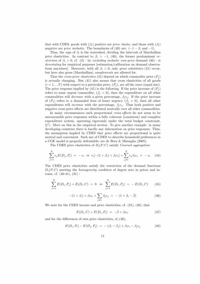
that with CDES: goods with (βi) positive are price elastic, and those with (βi)negative are price inelastic. The boundaries of (40) are: (−1 − βi and −1).

Thus, the sign of βi is the watershed, dividing the intervals of Marshallianprice elasticities. In contrast to βi > −1, (40), the former predominant re-striction of βi > 0, cf. (3) - by excluding inelastic own-price demand (40) - isdevestating for empirical purposes [estimation/calibration on demand observa-tions anywhere]. Moreover, with all βi > 0, only gross substitutes (41) occur,but here also gross (Marshallian) complements are allowed for.

Thus the cross-price elasticities (41) depend on which commodity price (Pj)is actually changing. But (41) also means that cross elasticities of all goods(i = 1, ...N) with respect to a particular price, (Pj), are all the same (equal size).The price response implied by (41) is the following. If the price increase of (Pj)refers to some urgent commodity, (βj < 0), then the expenditure on all othercommodities will decrease with a given percentage, βjej. If the price increaseof (Pj) refers to a demanded item of lesser urgency (βj > 0), then all otherexpenditures will increase with the percentage, βjej . Thus both positive andnegative cross price effects are distributed neutrally over all other commodities.

In many circumstances such proportional cross-effects do not seem to beunreasonable price responses within a fully coherent (consistent) and completeexpenditure system, operating rigorously under the total budget constraint,(C). More on this in the empirical section. To give another example: in manydeveloping countries there is hardly any information on price responses. Thus,the assumption implied by CDES that price effects are proportional is quiteneutral and convenient. Such use of CDES to describe household preferences ina CGE model is properly defendable; see de Boer & Missaglia (2005).

The CDES price elasticities of Di(P, C) satisfy Cournot aggregation:

N∑

j=1

ejE(Dj , Pi) = − ei ⇔ ei[−(1 + βi) + βiei] +

N∑

j 6=i

ejβiei = − ei (44)

The CDES price elasticities satisfy the restriction of the demand functionsDi(P, C) meeting the homogeneity condition of degree zero in prices and in-come, cf. (40-41), (31) :

N∑

j=1

E(Di, Pj) + E(Di, C) = 0 ⇔

N∑

j=1

E(Di, Pj) = − E(Di, C) (45)

−(1 + βi) + βiei +∑

j 6=i

βjej = − (1 + βi − β) (46)

We note for the CDES income and price elasticities, cf. (31), (40), that

E(Di, C) + E(Di, Pi) = −β + βiei (47)

and for the differences of own price elasticities, cf.,(40),

E(Di, Pi) − E(Dj , Pj) = − (βi − βj) + βiei − βjej (48)

11

Compared to (36), the sum/differences in (47), (48) are not exactly constant,but nearly so, when large number of commodities are involved (small ei).

Price elasticities (Slutsky) of CDES Hicksian demands, Yi = Hi(P, U)

The Slutsky - “compensated (Hicksian) demand” - elasticities, E(Hi, Pj), followdirectly from the Slutsky elements (derivatives), (22-23), and (31), (40-41) as:

E(Hi, Pi) = (Pi/Di)Sii = E(Di, Pi)+eiE(Di, C) = −(1+βi)+(1+2βi−β)ei < 0(49)

E(Hi, Pj) = (Pj/Di)Sij = E(Di, Pj)+ejE(Di, C) = (1+βi+βj−β)ej =

{

< 0> 0(50)

As far the “pure” (Hicksian) price responses (50) are concerned, there is con-siderable flexibility, both respect to the signs (complementarity, indifference,substitutability), and the numerical values of these “pure” cross-price elastici-ties. Behind the gross price elasticity values (40-41), there clearly exist freedomfor distinct ”income effects” and “substitution effects”, (49-50), of any pricechanges wihin the CDES demand/expenditure/budget system, (16), (18). Grosscomplements (41) may be Hicksian substitutes (50).

The utility level constraint associated with Hicksian demands Hi(P, U) issatisfied by CDES Slutsky elasticities, (49-50):

N∑

j=1

PjSji = 0 ⇔

N∑

j=1

ejE(Hj , Pi) = eiES(Yi, Pi) +∑

j 6=i

ejES(Yj , Pi) = 0

(51)

−ei(1 + βi) + ei(1 + 2βi − β)ei +∑

j 6=i

ej(1 + βi + βj − β)ei = 0 (52)

N∑

j=1

ejE(Hj , Pi) =N

∑

j=1

ej [E(Dj , Pi) + eiE(Dj , C)] = 0 (53)

A homogeneity of degree zero in prices for Hi(P, U) is met by CDES elasticities:

N∑

j=1

PjSij = 0 ⇔

N∑

j=1

E(Hi, Pj) = E(Hi, Pi) +∑

j 6=i

E(Hi, Pj) = 0 (54)

−(1 + βi) + (1 + 2βi − β)ei +∑

j 6=i

(1 + βi + βj − β)ej = 0 (55)

Allen partial elasticity of substitution of CDES Hicksian demands, Yi = Hi(P, U)

As gradually became clearer with the progress in economic science, there wereequivalent (“dual”) ways to describe consumer preferences and to obtain con-sumer demand systems. The neoclassical postulate underlying the derivation

12

of demand (Marshallian) systems was constrained utility maximization - MaxU(Y ), sub PY = C - which is here also a maintained hypothesis. However, evenfor analytically tractable parametrizations of the direct utility, U(Y ), the explicitform of the Marshallian demand functions, Di(P, C), could seldom be given, asDi(P, C) were only implicitly determined by solving the set of Lagrangian first-order conditions. Hence it turned out to be more convenient to assume thisconsumer max-problem actually solved and draw (check) some of its implica-tions, i.e parametrize instead an indirect utility function U = V (P, C) and useRoy’s identity to get the consumer (Marshallian) demand, Di(P, C) - as doneabove, (7), (16) with CDES. Moreover, besides explicitly obtaining Marshalliandemand functions Di(P, C) and the observable budget shares, ei(P, C) in termsof the indirect utility parameters (e.g., the “reaction parameters”, βi), we canstill analyze the substitution properties [implied by of U(Y )] by also calculatingall the relevant (Allen-partial) elasticities of substitution, (σij) in terms of theparameters of the indirect utility function, V (P, C). The key is the Slutskyequations of the derivatives (elasticities) connecting Marshallian and Hicksiandemands. The Slutsky equations must hold (“integrability conditions”) irrespec-tive of the alternative procedures (dual) for obtaining the Marshallian/Hicksiandemands. The Slutsky elements, Sij , (23) are symmetric, while the elasticities,ES(Yi, Pj), (50), are not symmetric, but substitution elasticities (σij) are to besymmetric.

The Allen partial elasticities of substitution, (σij), can be obtained by “nor-malizing” the Slutsky derivatives/elasticities, (22-23), (49-50), as:

σii = (C/DiDi) Sii = E(Hi, Pi)/ei = E(Di, Pi)/ei + E(Di, C) < 0 (56)

σij = (C/DiYj) Sij = E(Hi, Pj)/ej = E(Di, Pj)/ej + E(Di, C) =

{

< 0> 0

(57)N

∑

j=1

ejσji =

N∑

j=1

ejE(Hj , Pi)/ei =

N∑

j=1

ej [E(Dj , Pi)/ei + E(Dj , C)] = 0 (58)

N∑

j=1

ejσij =

N∑

j=1

E(Hi, Pj) =

N∑

j=1

E(Di, Pj) + E(Di, C) = 0 (59)

The aggregation property (58) is called the Allen aggregation, Allen (1938,p.504), and it is here seen to be satisfied as a combination of the Cournot aggre-gation (44) and Engel aggregation (33). Using symmetry of (σij), the restriction(59) now also follows from the homogeneity condition, cf. (45), (54).

As wellknown, the Allen elasticities of substitution, (σij) were originallynot obtained from Sij itself, but instead were derived from the (ij)-elementsof the inverse bordered Hessian matrix of the direct utility U(Y ), Allen (1938,p. 512, 504). Only later was Sij(P, C) of Marshallian demands obtained fromthe Hessian matrix of the expenditure function, C = e(P, U) in the context of

13

Hicksian demands,

∂Hi(P, U)

∂Pj= Sij(P, C) =

∂2e(P, U)

∂Pi∂Pj(60)

which fits the “normalization” and the Slutsky interpretation in (56-57), seeHanoch (1978, p. 290); cf. Takayama (1985, p. 144). The great analytical-economic advantage of indirect utility function U = V (P, C) is that also thesubstitution properties can be expressed explicitly in the parameters of V (P, C).

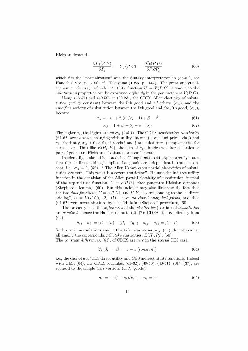
Using (56-57) and (49-50) or (22-23), the CDES Allen elasticity of substi-tution (utility constant) between the i’th good and all others, (σii), and thespecific elasticity of substitution between the i’th good and the j’th good, (σij),become:

σii = −(1 + βi)(1/ei − 1) + βi − β (61)

σij = 1 + βi + βj − β = σji (62)

The higher βi, the higher are all σij (i 6= j). The CDES substitution elasticities(61-62) are variable, changing with utility (income) levels and prices via β andei. Evidently, σij > 0 (< 0), if goods i and j are substitutes (complements) foreach other. Thus like E(Hi, Pj), the sign of σij decides whether a particularpair of goods are Hicksian substitutes or complements.

Incidentally, it should be noted that Chung (1994, p.44-45) incorrectly statesthat the “indirect addilog” implies that goods are independent in the net con-cept, i.e., σij = 0, (62). “ The Allen-Uzawa cross-partial elasticities of substi-tution are zero. This result is a severe restriction”. He uses the indirect utilityfunction in the definition of the Allen partial elasticity of substitution, insteadof the expenditure function, C = e(P, U), that generates Hicksian demands(Shephard‘s lemma), (60). But this incident may also illustrate the fact thatthe two dual functions, C = e(P, U), and U(Y ) - corresponding to the “indirectaddilog”, U = V (P, C), (2), (7) - have no closed analytical forms, and that(61-62) were never obtained by such ‘Hicksian/Shepard” procedure, (60).

The property that the differences of the elasticities (partial) of substitutionare constant - hence the Hanoch name to (2), (7): CDES - follows directly from(62),

σij − σkl = (βi + βj) − (βk + βl) ; σik − σjk = βi − βj (63)

Such invariance relations among the Allen elasticities, σij , (63), do not exist atall among the corresponding Slutsky elasticities, E(Hi, Pj), (50).The constant differences, (63), of CDES are zero in the special CES case,

∀i βi = β = σ − 1 (constant) (64)

i.e., the case of dual CES direct utility and CES indirect utility functions. Indeedwith CES, (64), the CDES formulas, (61-62), (49-50), (40-41), (31), (37), arereduced to the simple CES versions (of N goods):

σii = −σ(1 − ei)/ei ; σij = σ (65)

14

E(Hi, Pi) = −σ(1 − ei) ; E(Hi, Pj) = σej (66)

E(Di, Pi) = −σ(1− ei)− ei = −σ + (σ − 1)ei ; E(Di, Pj) = (σ − 1)ej (67)

E(Di, C) = E(Ci, C) = E(ei, C) + 1 = 1 (68)

If the pattern of income-, price-, and substitution elasticities in the CDES de-mand (expenditure) system may theoretically be viewed as rather restrictive,the range and scope in the CES system, (65-68), is evidently much narrower. Inaddtion to (68), the empirical drawback of CES is that the own-price elasticities(67) are all either larger or smaller than one, cf. βi > 0 above, (40). In relationto household budget survey data, the CES demand system makes no sense.

For the specification of consumer demands in applied (computable) generalequilibrium (CGE) models, the functional forms commonly used are CD, LESand CES, Shoven & Whalley (1992, p.95). A nesting structure for homoth-etic CES preferences can increase the scope for (65-67), but not at all for (68).For several purposes (consumer theory, interpretability, tractability), the moregeneral CDES demand system has certainly merits vis-a-vis alternative specifi-cations currently used in CGE models.

Fundamental Equation of Value Theory - Marshallian and Hicksian Demand

On this CDES background and its elasticity numbers, we next search for someclues about the magnitudes and general numerical pattern among various priceelasticities.

The Engel aggregation logically implies that some income elasticties are tobe larger and some other must be smaller than 1. No such numerical rule forthe size of elasticities are implied by the budget constraint for the set of own-price elasticities. They can all exceed one (elastic) or all be inelastic withoutlogically violating any conditions imposed by consumer demand theory or bud-get constraints. But own-price elasticities have several explicit relationshipsto cross-price elaticities and income elasticities that are useful for understand-ing/checking the actual numerical values of Marshallian own-price elasticities.

The Cournot aggregation implied by the budget constraint does give some in-dication about the connections between Marshallian price elastcities, mentionedby Marschak (1943, p. 27), and seen by rewriting (44) as,

ei [ 1 + E(Di, Pi) ] = − [

N∑

j 6=i

ej E(Yj , Pi) ] (69)

Thus, unless E(Di, Pi) = −1, the cross elasticities of the other commodities (Yj)with respect to own price (Pi) cannot all vanish; moreover, if E(Di, Pi) is elastic(inelastic), then at least one of the Marshallian cross price elasticities must beposetive (negative), i.e. be a gross (Marshallian) substitute (complement).

By the homogeneity of degree zero in prices and income, cf. (45), we have

E(Di, Pi) = − [N

∑

j 6=i

E(Di, Pj) ] − E(Di, C) (70)

15

E(Di, Pi) = E(Hi, Pi) − ei E(Di, C) (71)

E(Di, Pi) = − [

N∑

j 6=i

E(Hi, Pj) ] − ei E(Di, C) (72)

E(Di, Pi) = − [

N∑

j 6=i

ejσij ] − ei E(Di, C) = − [

N∑

j 6=i

ejσji ] − ei E(Di, C)

(73)E(Di, Pi) = eiσii − ei E(Di, C) = ei [ σii − E(Di, C) ] (74)

E(Di, Pj) = E(Hi, Pj) − ej E(Di, C) (75)

E(Di, Pj) = ejσij − ej E(Di, C) = ej [ σij − E(Di, C) ] (76)

Assuming no inferior goods, it is immediately seen from (70) that if the com-modity (Di) has a larger number of Marshallian substitutes (complements),then the absolute larger (smaller) becomes the Marshallian own-price elasticityof (Di). The homogeneity equation (70) also shows very clearly the fallacy intaking the income elasticty, E(Di, C), (with opposite sign) as an approximationto the Marshallian own price elasticity, E(Di, Pi). For, even if each of the crossprice elasticties, E(Di, Pj), is negligible, their sum is not necessarily negligible,since there is many of them. [That the sum in (47) is close to a nonzero constantis a particular property of CDES demand that obviously calls for some empiricalrelaxation in a further generalization of the indirect utility function, (7)].

Regarding the homogeneity (70), it seems worth stressing that Slutsky (1952,[equation (56); 1915 ]) demonstrated (70) - but in derivative form insteadof elasticities - as a consequence of the the symmetry relations (23); Schultz(1935, p.458) saw, (70), be “economically as probably the most signicant con-sequence” of Slutsky symmetry. As Hicksian and Allen aggregation above il-lustrated, symmetry together with Engel- and Cournot aggregation imply theMarshallian homogeneity property (70), a formula expressing in proper elastic-ities the Marshallian demand version of the decompostion of a price change intosubstitution(cross-price) effects and income effects.

Next, the ability of the so-called Hicksian (Slutsky) own-price elasticty,E(Hi, Pi), (49), to separate and properly absorb in (71) all the cross-priceelasticities of (70) is nontrivial either. But cross-price effects in (71) are onlyconcealed and reappear by homogeneity of Hicksian Yi(P, U), (56), (59), as

E(Hi, Pi) = eiσii = − [N

∑

j 6=i

ejσij ] = − [∑

j 6=i

E(Hi, Pj) ] (77)

By (70), (71), (77), we may also state the homogeneity property of Marshalliandemands by alternatively expressing (decomposing) the own-price elasticitiesas,

E(Di, Pi) = ei [ σii − E(Di, C) ] (78)

16

CDES literature comments

A few comments on the genesis of CDES demand add some further insights intoits system character and its natural place among other demand systems. Howdid it come about and what were the motivations ?

Leser (1941) wanted to measure the price and income elasticities of thedemand for various commodities. But the complete set of these elasticitiesshould satisfy the restrictions imposed by the theory of utility maximizationunder a budget constraint. The budget constraint implied that the set of income-and price elasticities of Marshallian demands must meet the restriction of Engelaggregation, (33), and Cournot aggregation, (44).

Then the symmetry imposed in terms of the Hicks-Allen relations (substitu-tion elasticities), gave the right-hand side of the equations (56-59), Leser (1941,p. 45) - cleverly adapted from Hicks & Allen (1934, p. 201). But like many oth-ers, he had little interest in the cross-price elasticities of demand, as the relevantnumber of alternative goods or composites to consider is an empirically difficultissue. However, the cross-price elasticities could not be ignored by just puttingthem equal zero, since then the Cournot aggregation (44) is violated, except forthe trivial case with also the own-price elasticities of minus one. Compatiblewith maximizing utility and a budget constraint, Leser (1941, p.43) assumed: “The cross-elasticities of demand depend only on the nature of the good whoseprice changes, and not on the nature of the good for which the effect is studied”- i.e., like (41), which together with (40) satisfies the Cournot aggregation (44).

Income elasticities that are all constant would not comply with Engel ag-gregation (33), except for unitary elasticity. Hence the traditional “double-logarithmic” expenditure functions (Engel curves) - cf. the power function innumerator of (16), (18), widely used and estimated for single commodities -could not be applied to all commodities in the budget and satisfy (33). How-ever, by combining these numerators with the suitable common denominatorexpression, cf. (16), (18), the parameter (βi) is no longer a constant incomeelasticity, but only a “reaction parameter” that particularly affects the demandelasticities of this good (i). Furthermore, the proper demand and budget func-tions, (16), (18), now generate varying income elasticities (31) that satisfy Engelaggregation (33). Evidently, the “reaction parameter” (βi) naturally stands outin the E(Di, C) formula and indeed, differences between the income elasticitiesof goods are solely determined by the differences of their respective “reaction co-efficients”, (36). By working from the budget formula (18) and through partialderivations, Leser (1941, p.49) obtained the income- and own- price elasticityformulas, stated in (31),(40). As he was not, beyond Cournot aggregation,interested in cross-price effects, he did not work out the CDES substitutionelasticities involved: (61-62). For the record, we mention that Leser in factobtained the lower boundary value (βi > −1), (40); Leser (1941, p. 49).

Houthakker (1960) studied the implications of assuming additivity of directand indirect utility functions for demand elasticities. The topic of this semi-nal paper was continued in Samuelson (1965, 1969), Houthakker (1965), Hicks(1969) and Hanoch (1975) with important issues for the understanding of the

17

CDES system.The additivity property of any indirect utility function was shown, Houthakker

(1960, p.250), generally to imply that the cross-price elasticies, E(Di, Pj), ∀i,are equal - i.e., it is not a special property of the additive CDES form (7), whichjust implied the distinct CDES parameter expression, (41). Regarding incomeelasticities, indirect additivity has the consequences, Hanoch (1975, p.410):

E(Di, C) − E(Dj , C) = σik − σjk (79)

The CDES parametric version of (79) was seen above in (63), (36).The implication of additivity of any direct utility function was that ratio

of cross-price elasticities is equal to the ratio of their income (C) elasticities,Houthakker (1960, p.248), cf. Deaton & Muellbauer (1980a, p. 138) :

E(Di, Pj)/E(Dk, Pj) = E(Di, C)/E(Dk, C) ; ∀i E(Di, Pj) 6= 0 ; N ≥ 3(80)

Generally, Marshallian cross-price elasticities are again here severely restrictedby additivity of the direct utility function, U(Y ). If some particular preferenceorderings were both directly and indirectly additive, then Houthakker noted thatall income elasticities must be equal, and hence unitary, i.e.,

[U(Y ) = V (P, C) ∧ additive] ⇒ E(Di, C) = 1 , i = (1, ..., N) (81)

The restrictions, (∀i E(Di, Pj) 6= 0 ; N ≥ 3), in (80) for obtaining (81)were added by Samuelson (1969, p. 357) in response to Hicks (1969). Cross-price elasticities of zero would render the left-hand side of (80) meaningless andfurther deductions from it vacuous. This exception of zero cross price elasticitiesis the CD case with both (dual) additive direct and indirect utility functions.The CD case - where (81) holds - must formally be treated separately to avoidindeterminate expressions, cf. (105), Appendix. Henceforth, the CD case is bythe restriction in (80) excluded from (81) and (82-87) below.

If the functional form with power functions was adopted for the so-called“direct addilog” utility function (with bi replacing βi), cf. (2), and Houthakker(1960, p.252),

U∗(Y ) =

N∑

i=1

a∗i (Yi)

bi ; ∀i bi 6= 0 (82)

then the ratio (80) becomes constant :

E(Di, Pj)/E(Dk, Pj) = E(Di, C)/E(Dk, C) = bi/ bk (83)

where the last equality easily followed from a consideration of the income elas-ticities, Houthakker (1960, p. 253).

Allen-partial elasticities of substitution for the pair of additive power spec-ifications were not considered in Houthakker (1960). The CES form (Arrow-Chenery-Minhas-Solow, 1961) had not yet appeared, and the multi-good CES

18

version came in Uzawa (1962). Regarding (82), we easily get by (57) and (83)the following expressions (the second by using symmetry):

σij/σkj = bi/ bk ; σij/σkl = (σij/σkj)(σjk/σlk) = (bi/ bk)(bj/ bl) (84)

The property that the ratios of the elasticities (partial) of substitution are con-stant made - CRES - the proper name for the Houthakker direct utility function(82). Gorman (1965) studied the general class of CRES functions, and par-ticular CRES subclasses were analyzed in Mukerji (1963) and Hanoch (1971,1975).

The constant ratios, (84), are equal to one in the special case,

∀i bi = b = (σ − 1)/σ (constant) , σ 6= 1 (85)

and the CRES specification, (82), is then reduced the CES direct utility function- with the set of CES elasticities given above, (65-68). In short, the special casesof CDES and CRES being dual CES preference orderings are, cf. (64), (85),

CDES = CES = CRES ⇔ [U∗(Y ) : bi = b] = [V ∗(P, C) : βi = β] (86)

or[ U(Y ) = V (P, C) ∧ additive ] ⇔ [ σij = σ ] (87)

The CES form of the direct/indirect utility functions is the only functional formwith the property of self-duality. The only way indirect additivity (includingCDES) and direct additivity (including CRES) can be dual (equivalent prefer-ences) is by both additivities collapsing to CES form, (87). A nice and importantparametric pair of CES forms occurs with the value: σ = 2, cf. (85), (82), (105),Samuelson (1965, p.795), Solow (1956, p.77), Jensen & Larsen (2005, p.78):

U(Y ) =N

∑

i=1

(αiYi)1

2 ⇔ V (P, C) =N

∑

i=1

αi (C/Pi) (88)

Since constant returns to scale is a predominant property of long-run productionfunctions, CES and CRESH (homogeneity restricted CRES), Hanoch (1971), arenatural elements of the supply side in CGE models. For consumption (demandside) however, CES and any homothetic preferences, (81) would jettison solidempirical and observable evidence on budget shares from budget studies sinceEngel (1857). CDES represents nonhomothetic preferences - C can formally notbe separated in (7), except for (86) - which is one of its fundamental meritsamong tractable preference orderings.

The approach to demand analysis and expenditure systems by Somermeyeret al (1956, 1972) was that of “flexible functional form“ under the maintainedhypothesis of constrained utility maximization. By experimenting with linear,hyperbolic, power, and exponential specifications and their respective parame-ter restrictions, it turned that the nonlinear power specification was desirablefrom several criteria, parsimony of parameters, ease of interpretation, compu-tational ease and sensible robustness outside the range of observed data. That

19

the power specification is flexible and hard to replace for demand functions tobe derivable from a utility function was noted by Arrow (1961, p. 177). Thusthe demand functions (budget shares) (16), (18) came into focus, and their rel-evant parameter intervals was to be scrutinzed. The non-negativity of demand(Di) for every non-negative price and income (C) was ensured by positive (αi),(16); this restriction is involved with the monotonicity requirements (9-11). Thesecond-order Slutsky conditions (negative semi-definiteness of the substitutionmatrix),(9-11) implied the restrictions on (βi) - as obtained by Van Driel (1974)mentioned above. Essentially these restrictions imposed by the maintained hy-pothesis of an underlying (unknown) strictly quasi-concave direct utility functionis by duality reflected in condition (14) of strictly quasi-convexity of the explicitindirect utility function of CDES. A hard and long story of empirical work andexperimentation is now codified in the proper intervals of the parameters in (7).

Part II : Application

5. Estimation of reaction parameters from budget surveys

The consumer prices here do not vary, and they are the same for all households;we add an index (h = 1, · · ·H) to denote households. Hence the CDES budgetshare equations (18) of the households are :

eih =αi(Ch/Pi)

βi

∑Nj=1 αj(Ch/Pj)βj

(89)

Wit (1957, 1960) proposed selecting a reference commodity (which without lossof generality is the first one), and using the following transformation of (89):

log

(

eih

e1h

)

= log eih − log e1h = γi + (βi − β1) log(Ch) + εih i = 2, · · · , N (90)

where εih is the disturbance term, and where the constant term is,

γi = log αi − log α1 − (βi log Pi − β1 log P1) (91)

It follows from (90) that with this procedure we can only estimate the differencesof the “reaction parameters” of interest, βi − β1.

By defining,

yi =

(log ei1 − log e11)...

(log eiH − log e1H)

; X =

1 log C1

......

1 log CH

; (92)

β∗i =

[

γi

βi − β1

]

; εi =

εi1

...εiH

20

we can rewrite (90) as:

yi = Xβ∗i + εi i = 2, · · · , N (93)

i.e. to a seemingly unrelated regression (SUR) model with identical explanatoryvariables - for which it is known that ordinary least squares (applied to eachequation separately) is efficient, (Heij et al., 2004, p.687).

Due to problems of data availability, the reference commodity will vary be-tween countries (and periods); but irrespective of the particular choice of ref-erence commodity, comparison of results is simple, as each set of parameterestimates can consistently be transformed to another reference by,

(βi − β1) − (βm − β1) = βi − βm (94)

Hence the actual choice of reference commodity does neither affect the calcula-tion of income (C) elasticities. Moreover, if just one estimated price elasticitywas known from other sources, then we can calculate the corresponding reactionparameter estimate from (40-41) - which together with the estimated differences(93) will give us the absolute values of all reaction parameters (βi). Thereby, thecomplete set of CDES price elasticities can be derived, as we shall demonstrate.

6. Budget Shares, Estimates of βi − β2 and E(Di,C)

Classification of consumer goods(services) and social strata

The universal human wants (needs) have, in various amounts, included at leastthree main categories of consumer goods: 1. Food, 2. Clothing, 3. Shelter.

As to the provision for other wants and fancies, Adam Smith (p.34) says:“Every man is rich or poor according to the degree in which he can afford toenjoy the necessaries, conveniences, and amusements of human life.”

In more detail on these wants and fancies, Smith (pp.182-183) continues:“Cloathing and lodging, household furniture, and what is called equipage, arethe principal objects of the greater part of those wants and fancies. The richman consumes no more food than his poor neighbor. In quality it may be verydifferent, and to select and prepare it may require more labor and art; but inquantity it is very nearly the same.

But compare the spacious palace and great wardrobe of the one, with thehovel and the few rags of the other, and you will be sensible that the differencebetween their cloathing, lodging, and household furniture, is almost as great inquantity as it is in quality. The desire for food is limited in every man by thenarrow capacity of the human stomach; but the desire of the conveniencies andornaments of building, dress, equipage, and the household furniture, seems tohave no limit or certain boundary.”

Budget surveys have until 1970’s often exclusively focused on the expenditurepatterns (“standard of living costs”) of employee households (wage and salaryearners), since a subsidiary purpose was to obtain “weights” (ei) for the calcu-lation of various official price indexes that regulated nominal wage contracts.

21

Hence, less variation in ornaments of lodging and dress, etc., (“life styles”) areexpected for such households than those quoted from Adam Smith. But his clas-sification of goods into: necessaries, conveniences, and amusements resemblesmodern measurements by income elasticities, E(Di, C): below, around, largerthan unity, as the budget constraint (Engel aggregation) implies.

The classification of consumer goods and services that was used in the Dan-ish Consumer Survey (employee households) of 1971, is shown in Table 1. Itcovers seven main categories: 1. Food and Beverages 2. Clothing and Footwear3. Housing 4. Dwelling Operations 5. Medical Care and Health 6. Leisure7. Transport. Each category consists of a varied set of sub-items; the com-plete expenditure pattern is described by a total number (N) of 41 items. Thecoresponding 41 budget shares, (ei), for two life-cycle groups (junior-/seniorfamilies), is seen in Table 1.

The sampling design and random selection of around 1000 household inthe 1971 survey from 1 million employee households may briefly be described.The households were interviewed, made detailed expenditure accounting for onemonth, and they were successsively chosen throughout the year to offset seasonalinfluence on spending patterns. The stratifications of household units were basedon several criteria: geography (metropolitan, provincial), age of members andnumber of children, social groupings (occupational status in private and publicsector). We have here chosen to use the budget shares from a demographic typeof the household stratification into 8 life-cycles groupes; but only two groupesare shown in Table 1. The junior families have only children below 7 years,whereas the senior families include no longer any children and the house wife isabove 45 years - these senior households are not retired (pensioners), as at least50 percent of the total income of any household in this consumer survey mustbe factor (wage, salary) income.

Factor Income and Transfers (welfare, children allowances, unemploymentbenefits) gives Gross Income. The latter with deductions of Direct Taxes (in-come, real estate, social insurance) gives Disposable Income, which is splitbetween Total Consumption (C) and Gross Saving (S). The published bud-get shares of various consumer expenditure usually have disposable income asthe denominator. Since the relationship between Disposable Income and GrossSaving varies across life-cycle groupes, the differences in consumer expenditurepatterns are, theoretically and empirically, more adequately described (and re-calculated by us) as budget shares with the total consumption (C) as denom-inator. Table 1 shows the average budget shares (ei) of the life-cycle groupeswith their respective average (yearly) totals (C) : 42557 DKK and 40831 DKK.

Regarding the expenditure pattern of the junior and senior families in ta-ble 1, we cannot be surprised to see that budget shares of (milk products) and(beer,wine) are significantly higher (lower) for the junior families; the seniorsenjoys higher quality foods at home (meat,9) and outside (restaurants,35). Thehousing cost (gross rents,17) takes a higher toll on the young families. Health ex-penditures (medical products,29) are slightly higher for the seniors. Apart fromthe items mentioned, the average budget shares of the two life-cycles groupesare overall remarkly similar. Cars (transport equipment, insurance,auto repairs,

22

gasoline,41,39-37) became significant budget items for both the juniors and se-niors in the years around 1971. The expenditures on transport equipment (41)[like housing,(19)] refer “user cost” of these physical assets [i.e.,not to their as-set (purchase) price]. The “user costs” are not calculated as “imputed rents(services)”, but made up of cash payments on down-payments, consumer credit,mortgage interest that are recorded with renting (owning) these durable assets.

Within the two life-cycle groupes, several sampling units will have zero ex-penditures on a number of the items listed in Table 1; there are non-smokers,some are vegetarians, other eschew alcholic beverages, and many have no auto-mobiles. In terms of consumer modelling, the nonzero budget shares in Table 1each refer to budget shares of a representative consumer, evaluated at, respec-tively, (C = 42557, C = 40831). The main categories (subtotals, Table 1) inthe Danish expenditure pattern for employee household in 1971 are similar tothose for employees in other Scandinavian countries at that time (Sweden,1969,Norway, 1973), cf. SU (1977, p.226).Remark 1. Former Budget Studies. Sampling surveys of budget data fromemployee household have been collected and compared by government agenciesfor a long time. A single table of budget shares from the first and most famous,Engel (1857), of all family expenditure studies is quoted here in Table 1 A,because it has acted as benchmark for later inquiries, and because it is seldomseen anywhere in the literature, except

23

Table 1: Classification of Consumer Goods and Servicesand Budget Shares (100 ei , i = 1, ... 41) of Social Strata.

Junior SeniorFamilies Families

1. Food and Beverages:

1 Bread (cereals) 2.44 2.392 Butter 0.64 0.763 Margarine (fats, oils) 0.64 0.654 Sugar (confectionary) 0.85 0.985 Milk (cream, yoghurt) 2.23 1.636 Cheese (curd) 0.64 0.767 Other foods 1.81 2.178 Vegetables (fruits) 3.08 3.049 Meat 5.63 7.27

10 Fish 0.64 0.9811 Coffee (tea, cocoa) 1.38 1.9512 Soft drinks (mineral water) 0.53 0.7613 Beer 1.27 1.8414 Wine and spirits 0.96 1.7415 Tobacco products 3.50 3.80

Sum 1-15: 26.24 30.72

2. Clothing and Footwear:

16 Clothing 5.73 5.8617 Footwear (shoes, boots) 1.38 0.98

Sum 16-17: 7.11 6.84

3. Housing:

18 Fuel (gas, liquids) and light 4.25 4.4519 Gross rents (water rates, mortgage) 17.62 12.04

Sum 18-19: 21.87 16.49

24

Junior SeniorFamilies Families

4. Dwelling Operations:

20 Glassware (tableware, utensils) 0.96 0.7621 Household textiles (furnishings) 0.85 0.9822 Household machines (appliances) 1.70 1.0823 Furniture (fixtures, carpets) 3.61 3.4724 Non-durable household goods 2.12 2.1725 Household services (domestic services) 0.85 0.5426 Communication (post, telephone) 0.96 1.4127 Radio and television sets 1.17 1.7428 Miscellanous (services n.e.c.) 4.46 2.82

Sum 20-28: 16.68 14.97

5. Medical Care and Health:

29 Medical and pharmaceutical products 0.53 1.0830 Medical services (physicians, nurses) 0.85 0.8731 Personal care (barber, beauty shops) 1.27 1.63

Sum 29-31: 2.65 3.58

6. Leisure:

32 Personal goods (jewellery, watches, rings) 0.96 0.8733 Leisure equipment (camera, musical, boats) 2.65 3.1534 Entertainment (comfort, cultural services) 2.23 3.1535 Restaurants (cafes, hotels, lodging services) 1.49 3.8036 Books and papers (magazines) 2.12 1.95

Sum 32-36: 9.45 12.92

7. Transport:

37 Gasoline (oil) 3.61 3.1538 Auto repairs (transport equipment) 2.55 2.1739 Other transport expenses (insurance, taxes) 2.44 2.1740 Transport services (bus, train, taxi, rent) 1.70 1.9541 Transport equipment (vehicle purchases) 5.73 5.10

Sum 37-41: 16.03 14.54

Sum 1-41: 100.00 100.00

Total Consumption Expenditures (average) DDK 42557 40831

Source: Statistiske Undersgelser No. 34, Copenhagen (1977, p. 238-45).

25

Marshall (1920). We have changed Marshall’s item descriptions a little bit - inaccordance with Engel’s original expenditure classification; cf. Stigler (1954, p.98) on the origin of the Engel data and the early collections of budgetary datain Europe and USA. By induction and the evidence of Table 1A, Engel (1857,p. 28) felt justified to state as a general empirical law: “ The poorer a familyis, the larger share of the total expenditures must be allotted to the provisionof nourishment (nahrung, food)”. Engel’s law has never been refuted anywhere,and is confirmed in all subsequent surveys, Houthakker (1957), irrespective ofclimatic or cultural conditions. As stressed by Engel (1857, p. 33), the generallaw refers to the budget share and not to the level (absolute size) of the foodexpenditures - which in fact were 66% higher for family type (150− 200£) thanthe level in family type (45 − 60£).

The variations of the budget shares with income for other items in Table1A also reflect some basic patterns and historical tendencies (with exceptionsand gradual shifts) observed ever since in many empirical consumer demandstudies. The structural consistency exhibited by consumption patterns is ofgreat importance from the viewpoints of demand theory, empirical methods, andapplications. In accordance with these assumptions, a thorough investigationof family budget data and market statictics was carried out by Wold & Juren(1952) so as to obtain a unified historical description of the demand structurein Sweden; one picture of their budget data is shown in Table 1B. Finally, theaverage budget shares of income groupes in Leser’s paper are given in Table 1C.

A remarkable feature of the Tables: 1 - 1C, is the stability of the budgetshare for the item, Fuel & Light, in 150 years. The budget shares of Clothingin Table 1A-1B imply for a long time an income elasticity slightly below one.The high income elasticity of housing is a characteristic feature of demand inScandinavia as is already evident from budget shares in Table 1B.

For the income (disposable) variable, the frequency distribution of the sam-pling units (households) within the two life-cycle groupes of Table 1 are shownin Table 1D. For each of these income intervals for Junior and Senior families,we could as in Table 1 calculate all the average budget shares; their patternwould look similar to Table 1A-1C - with also Engel’s law always confirmed.

However, instead of tabulating 41 budget shares by discrete income (to-tal expenditure) intervals, the entire sample of the respective Junior and Seniorfamilies are now used to estimate the CDES parameters, cf.(90), with here butter(j = 2) as reference commodtiy. The estimated parameters, ranked accordingto size for both life-cycle groupes, are shown in Table 2. We have given theparameter estimates without indicating the standard errors (or t-values) in Ta-ble 2; they are availlable in Jensen (1980, p.283-85), but here omitted as suchstandard deviations carry little weight as economic-statistical significance indi-cators, on grounds explained by Wold (1952, p. 260). Statistically, estimatesthat are closer to zero (middle of Table 2) are less significant than large negative(positive) parameter estimates at the end of the rankings. Economically, therange of the reaction parameters (βi), (13), place many item values meaningfulclose to zero.

26

Table 1A. Budget Shares of Social Strata : Saxony 1857.

Proportions of the Expenditure of the Family of-

Items of ExpenditureWorkman with an Workman with an Workman with anyearly income of yearly income of yearly income of

45 - 60 £ 90 - 120 £ 150 - 200 £

1 Food (beverage, tobacco, taverns) 62.0 55.0 50.02 Clothing (footwear, jewellery) 16.0 18.0 18.03 Lodging (rent, utensils, furniture) 12.0 12.0 12.04 Light and Fuel (wood,coal, gas,oil) 5.0 5.0 5.05 Education (culture, church) 2.0 3.5 5.56 Public Protection (taxes) 1.0 2.0 3.07 Care of Health (medical, pharma) 1.0 2.0 3.08 Personal Services 1.0 2.5 3.5

Totals 100.0 100.0 100.0

Source: Marshall (1920, p. 115); Engel (1857, 1895, p. 30).

Table 1B. Budget Shares of Social Strata : Sweden 1913-1933.

Industrial worker families Middle class familiesItem group

1913 1923 1933 1923 19331 Nourishment 50.4 47.8 40.0 31.5 28.52 Clothing 14.2 16.0 14.6 14.5 14.43 Fuel, Light, Laundry 6.4 6.5 6.1 6.2 6.04 Housing 13.3 11.6 16.9 13.5 18.25 Furniture (furnishings) 4.7 4.8 5.2 7.1 6.46 Personal Services (domestic) 1.0 0.5 0.4 4.2 3.37 Hygiene (medical care) 1.8 2.3 3.2 2.8 3.38 Education (culture, travel) 5.0 6.2 7.0 9.2 9.79 Other Expenditures 3.1 4.2 6.6 11.0 10.2

All expenditures 100.0 100.0 100.0 100.0 100.0

Source: Wold (1952, p. 20); Recalculation with all expenditures = C.

Table 1C. Budget Shares : Families in the U.S.A. 1918-19

Item group 100 ei

1 Food 38.92 Clothing 16.23 Fuel, Light 5.44 Rent 13.65 Furnishings 5.06 Miscellaneous 20.9

Total 100.0

Source: Leser (1941, p. 53).

27

In judging the validity and reliability of the parameter estimates, a main crite-rion will the overall consistency obtained for the different budget items withinand between social strata, and proper comparisons and checks with specific evi-dence from other sources and periods. Looking at the point estimates in Table 2for the two family types, a main feature of the results is that a stable hierarchyexists between the item groupes in their preference and demand sensitivity, aswas evident in budget shares of Table 1 discussed above.

The CDES expenditure (“income”) elasticities of the 41 consumer goods andservices, satisfying Engel aggregation, are shown in Table 3. The methods andformulas employed in calculating the elasticities in Table 3 from Table 1 andTable 2 have been explained above in section 3. Hence with butter (j = 2) asreference commodity of the estimates in Table 2 and (32), we get for butter

E(D2, C) = 1 −

41∑

i=1

ei(βi−β2) = 1 − β2 = 1 − 0.48614 = 0.51386 (95)

for the Junior families, and for the Senior families :

E(D2, C) = 1 − β2 = 1 − 0.19075 = 0.80925 (96)

- evaluated at, respectively, (C = 42557, C = 40831). All the other elasticitiesin Table 3 are then calculated from (36), (95),(96), and Table 2 as, respectively,

E(Di, C) = E(D2, C) + βi − β2 = 0.51386 + βi − β2 (97)

E(Di, C) = 0.80925 + βi − β2 (98)

The main feature of the results obtained in Table 3 (with the same ranking asin Table 2) is the overall similarity that subsists between the commodity classesin their expenditure (income) sensitivity for the two life-cycle groupes (apartfrom some obvious differences already mentioned, cf. Table 1). Since the sampleaverage of C was higher for the Junior groupe, the item elasticities E(Di, C)should ceteris caribus be smaller for the Junior families, cf. (25), (32), and theirsize in Table 3 comply with such tendency.

Several food items are among the necessities with the lowest elasticities,although fancy food also exists among the luxuries for both groups (rank 31, 35).Clothing, footwear, and goods and services associated with dwelling operationshave elasticities around one. Housing, furniture, and cars are the high elasticitygoods for Juniors, and latter good also tops the list for the Senior families.The CDES elasticities in Table 3 display a pattern and numerical values thatconform with the general picture of abundant empirical demand studies.

28

Table 2 : Ranking of the Reaction Parameter Estimates: (βi − β2)

Junior Families Senior Families

Rank Commodity Class βi − β2 Rank Commodity Class βi − β2

1 Bread -0.29404 1 Margarine -0.562342 Margarine -0.25465 2 Bread -0.394383 Sugar -0.24830 3 Coffee -0.337234 Coffee -0.21253 4 Miscellaneous -0.255525 Tobacco -0.20813 5 Fuel and light -0.231226 Milk -0.12385 6 Tobacco -0.249247 Fuel and light -0.06171 7 Soft drinks -0.238928 Butter - 8 Personal goods -0.187899 Radio, tv sets 0.01635 9 Meat -0.18665

10 Medical products 0.04118 10 Medical products -0.1027611 Other nondurable goods 0.09349 11 Other nondurable goods -0.0935512 Cheese 0.09450 12 Household machines -0.0792013 Household textiles 0.10560 13 Milk -0.0574914 Vegetables 0.11840 14 Medical services -0.0491115 Meat 0.12885 15 Beer -0.0488816 Household machines 0.15462 16 Books and papers -0.0234517 Glassware 0.20301 17 Fish -0.0082918 Fish 0.23152 18 Butter -19 Soft drinks 0.27881 19 Cheese 0.0320020 Leisure equipment 0.34423 20 Entertainment 0.0612021 Beer 0.34631 21 Household textiles 0.0724422 Entertainment 0.37195 22 Personal care 0.0888823 Auto repairs 0.37212 23 Furniture 0.0968424 Clothing 0.38976 24 Sugar 0.0999025 Gasoline 0.42036 25 Auto repairs 0.1216426 Footwear 0.43999 26 Vegetables 0.1242927 Personal goods 0.54508 27 Glassware 0.1391228 Medical services 0.58257 28 Gross rents 0.1793629 Wine and spirits 0.58607 29 Footwear 0.2473330 Personal care 0.60113 30 Other transport 0.2973631 Other foods 0.64302 31 Transport services 0.3418632 Other transport 0.66149 32 Clothing 0.3709933 Books and papers 0.68632 33 Radio, tv sets 0.3925434 Gross rents 0.71112 34 Gasoline 0.4221835 Restaurants 0.74708 35 Other foods 0.4533536 Household services 0.78325 36 Wine and spirits 0.6457237 Miscellaneous 0.86186 37 Leisure equipment 0.6950038 Transport services 0.91800 38 Household services 0.7097339 Furniture 1.04451 39 Communication 0.8991140 Communication 1.33410 40 Restaurants 1.0242041 Transport equipment 1.78225 41 Transport equipment 1.32967

β2 =∑

41

i=1ei(βi − β2) 0.48614 β2 =

∑

41

i=1ei(βi − β2) 0.19075

29

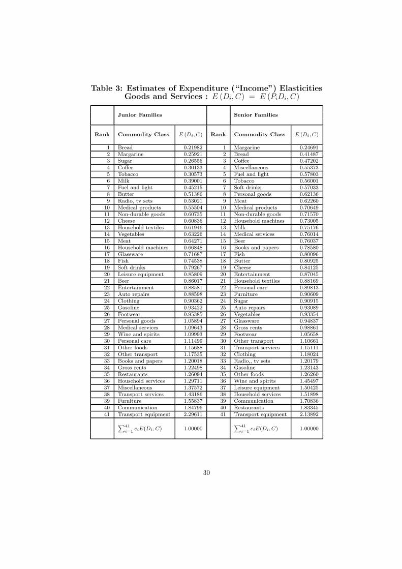
Table 3: Estimates of Expenditure (“Income”) ElasticitiesGoods and Services : E (Di, C) = E (PiDi, C)

Junior Families Senior Families

Rank Commodity Class E (Di, C) Rank Commodity Class E (Di, C)

1 Bread 0.21982 1 Margarine 0.246912 Margarine 0.25921 2 Bread 0.414873 Sugar 0.26556 3 Coffee 0.472024 Coffee 0.30133 4 Miscellaneous 0.553735 Tobacco 0.30573 5 Fuel and light 0.578036 Milk 0.39001 6 Tobacco 0.560017 Fuel and light 0.45215 7 Soft drinks 0.570338 Butter 0.51386 8 Personal goods 0.621369 Radio, tv sets 0.53021 9 Meat 0.62260

10 Medical products 0.55504 10 Medical products 0.7064911 Non-durable goods 0.60735 11 Non-durable goods 0.7157012 Cheese 0.60836 12 Household machines 0.7300513 Household textiles 0.61946 13 Milk 0.7517614 Vegetables 0.63226 14 Medical services 0.7601415 Meat 0.64271 15 Beer 0.7603716 Household machines 0.66848 16 Books and papers 0.7858017 Glassware 0.71687 17 Fish 0.8009618 Fish 0.74538 18 Butter 0.8092519 Soft drinks 0.79267 19 Cheese 0.8412520 Leisure equipment 0.85809 20 Entertainment 0.8704521 Beer 0.86017 21 Household textiles 0.8816922 Entertainment 0.88581 22 Personal care 0.8981323 Auto repairs 0.88598 23 Furniture 0.9060924 Clothing 0.90362 24 Sugar 0.9091525 Gasoline 0.93422 25 Auto repairs 0.9308926 Footwear 0.95385 26 Vegetables 0.9335427 Personal goods 1.05894 27 Glassware 0.9483728 Medical services 1.09643 28 Gross rents 0.9886129 Wine and spirits 1.09993 29 Footwear 1.0565830 Personal care 1.11499 30 Other transport 1.1066131 Other foods 1.15688 31 Transport services 1.1511132 Other transport 1.17535 32 Clothing 1.1802433 Books and papers 1.20018 33 Radio,, tv sets 1.2017934 Gross rents 1.22498 34 Gasoline 1.2314335 Restaurants 1.26094 35 Other foods 1.2626036 Household services 1.29711 36 Wine and spirits 1.4549737 Miscellaneous 1.37572 37 Leisure equipment 1.5042538 Transport services 1.43186 38 Household services 1.5189839 Furniture 1.55837 39 Communication 1.7083640 Communication 1.84796 40 Restaurants 1.8334541 Transport equipment 2.29611 41 Transport equipment 2.13892

∑

41

i=1eiE(Di, C) 1.00000

∑

41

i=1eiE(Di, C) 1.00000

30

7. Reaction Parameters, Price and Substitution Elasticities

The information about the estimated differences (βi −β2) in Table 2 were suffi-cient for calculating income elasticities of CDES demand, (16), (97); adding anarbitrary constant to all the βi - parameters would not change the elasticity withthe respect to C in (16) - whereas any particular price elasticity would clearlybe affected by such additive constant in every βi. Thus CDES price elasticitiescannot be calculated from Table 2; moreover, the ’reaction parameters’(βi) can-not be fully recovered from just family budget surveys (expenditure data). Butthey are as ’invariances’ (basic parameters) - in contrast to continuously chang-ing income and price elasticities - the ultimate empirical objective to obtain forthe CDES indirect utility function and demand system, (7), (16).

As mentioned at the end of section 5, extraneous information (literaturesurveys, benchmark observations, calibration procedures) on any single priceelasticity will in combination with Table 2 allow full identification and estimationof all the parameters, (βi). Our parameter calibrations will be based on the priceelasticity of butter that is a well-defined homogeneous good and a classic articleof many demand studies - convenient also as being our reference commodity.

Hence by (16), the reaction parameter for butter will be calibrated as

β2 = [E(D2, P2) − 1]/(1 − e2) (99)

Market statistics in the form of time series are often seen as the principal mate-rial for the estimation of direct price and cross price elasticities. However, ourelasticity and parameter in (99) do not refer to total butter market demand,but instead to butter demand elasticities segmented to our life-cycle groups.Accordingly information from specialized demand studies are called for ; suchfood demand analyses are available, since our life cycle categories have beenstandard for a long time in many countries.

Calculations of β2 by (99) - for different butter price elasticities and with e2

from Table 1 - are collected in Table 4a. The starred price elastities appear asthe most plausible ones for several reasons. They are partly in line with butterelasticities seen for our family types in Wold & Juren (1952, p. 266-69, 285-88),conform properly with the income elasticities, (95),(96), and fit in appropriatelywith the wider implications of the corresponding β2 (and β) values upon all theother price elasticities, as explained below.

Table 4a. Reaction Parameter β2, β, and E(D2,P2).

Junior Families Senior Families

E(D2, P2) β2 β E(D2, P2) β2 β

-0.9 -0.10064 0.38550 -0.9* -0.10066 0.09009-0.8 -0.20128 0.28486 -0.8 -0.20131 -0.01056-0.7* -0.30192 0.18422-0.6 -0.40256 0.08358

31

Table 4: Ranking and Size of Reaction Parameter Estimates: (βi)

Junior Families Senior Families

Rank Commodity Class βi Rank Commodity Class βi

1 Bread -0.59596 1 Margarine -0.663002 Margarine -0.55657 2 Bread -0.495043 Sugar -0.55022 3 Coffee -0.437894 Coffee -0.51445 4 Miscellaneous -0.356185 Tobacco -0.51005 5 Fuel and light -0.331886 Milk -0.42577 6 Tobacco -0.349907 Fuel and light -0.36363 7 Soft drinks -0.339588 Butter -0.30192 8 Personal goods -0.288559 Radio, tv sets -0.28557 9 Meat -0.28731

10 Medical products -0.26074 10 Medical products -0.2034211 Non-durable goods -0.20843 11 Non-durable goods -0.1942112 Cheese -0.20742 12 Household machines -0.1798613 Household textiles -0.19632 13 Milk -0.1581514 Vegetables -0.18352 14 Medical services -0.1497715 Meat -0.17307 15 Beer -0.1495416 Household machines -0.14730 16 Books and papers -0.1241117 Glassware -0.09891 17 Fish -0.1089518 Fish -0.07040 18 Butter -0.1006619 Soft drinks -0.02311 19 Cheese -0.0686620 Leisure equipment 0.04231 20 Entertainment -0.0394621 Beer 0.04439 21 Household textiles -0.0282222 Entertainment 0.07003 22 Personal care -0.0117823 Auto repairs 0.07020 23 Furniture -0.0038224 Clothing 0.08784 24 Sugar -0.0007625 Gasoline 0.11844 25 Auto repairs 0.0209826 Footwear 0.13807 26 Vegetables 0.0236327 Personal goods 0.24316 27 Glassware 0.0384628 Medical services 0.28065 28 Gross rents 0.0787029 Wine and spirits 0.28415 29 Footwear 0.1466730 Personal care 0.29921 30 Other transport 0.1967031 Other foods 0.34110 31 Transport services 0.2412032 Other transport 0.35957 32 Clothing 0.2703333 Books and papers 0.38440 33 Radio,, tv sets 0.2918834 Gross rents 0.40920 34 Gasoline 0.3215235 Restaurants 0.44516 35 Other foods 0.3526936 Household services 0.48133 36 Wine and spirits 0.5450637 Miscellaneous 0.55994 37 Leisure equipment 0.5943438 Transport services 0.61608 38 Household services 0.6090739 Furniture 0.74259 39 Communication 0.7984540 Communication 1.03218 40 Restaurants 0.9235441 Transport equipment 1.48033 41 Transport equipment 1.22901

β =∑

41

i=1eiβi 0.18422 β =

∑

41

i=1eiβi 0.09009

32

This selection of (β2) from Table 4a together with Table 2 finally give thesizes for the complete set of reaction parameters, listed in Table 4. Meaningfulinterpretation and comparison between the numbers for junior/senior familieswere not possible (despite correct ranking) in Table 2, as β2 was unknown andmight be widely different for such life-cycle groupes. Overall the numbers inTable 4 now look more similar (min, range) for the two family types, althoughnatural differences in their preferences still exist. As to Junior families, thesix items at the top of the table are more ’urgent necessities’ than those ofthe Seniors. On the other hand, the average urgency (rigidity) level (β) issomewhat lower for the Juniors, respectively. The location and different sizes ofitem specific reaction parameters (βi) will affect the pattern of price elasticitiesof demand for the two family types.

The Marshallian and Slutsky price elasticities (own, cross), and the Allensubstitution elasticities - calculated from Table 4 and Table 1 according to theirparametric formulas given in section 3 - are together with income elasticitiesexhibited for the respective life-cycle groupes in Tables 5A-5B, Tables 6A-6B.For ease of discussion and numerical accuracy evaluations, the item budgetshares (100ei) are included in these tables - as are the exact consistency checksby the Engel and Cournot aggregations and homogeneity restrictions.

As seen from the listed own-(direct) price elasticities of commodities in Table5A and Table 6A, the Marshallian and Slutsky own-price elasticities have nearlythe same size (differing in most cases only on second decimals). Evidently, the“income effect” of own-price changes upon Marshallian price elasticities arevery small, when a large number of commodities (and hence individually smallbudget shares) are involved, cf. (49). Since no inferior goods were actuallyobserved (estimated) for neither Junior nor Senior families in Table 3, all theMarshallian price elasticities in Tables 5A and Table 6A are abslolutely largerthan the corresponding Slutsky (“compensated”) elasticity.

We see for CDES income and price elasticities, Tables 5A, 6A, cf. (31), (40),

E(Di, C) + E(Di, Pi) = −β + βiei ; β = 0.18422, β = 0.09009 (100)

and for the differences of price elasticities, cf. (40),

E(Di, Pi) − E(Yj , Pj) = − (βi − βj) + βiei − βjej (101)

Compared to (36), the sum/differences in (100), (101) are not exactly constant,but nearly so, when large number of items are involved (small ei).

33

Table 5 A. Junior Families : Income- and Own-Price Elasticities.

R Commodity Class 100ei E(Di, C) E(Di, Pi) E(Hi, Pi) σii

1 Bread 2.44161 0.21982 -0.41859 -0.41322 -16.924092 Margarine 0.63694 0.25921 -0.44697 -0.44532 -69.915393 Sugar 0.84926 0.26556 -0.45445 -0.45219 -53.245904 Coffee 1.38004 0.30133 -0.49265 -0.48849 -35.396605 Tobacco 3.50318 0.30573 -0.50782 -0.49710 -14.190086 Milk 2.22930 0.39001 -0.58372 -0.57502 -25.793947 Fuel and light 4.24628 0.45215 -0.65181 -0.63261 -14.897928 Butter 0.63694 0.51386 -0.70000 -0.69673 -109.386149 Radio, tv sets 1.16773 0.53021 -0.71776 -0.71157 -60.93629

10 Medical products 0.53079 0.55504 -0.74064 -0.73769 -138.9817111 Non-durable goods 2.12314 0.60735 -0.79599 -0.78310 -36.8838912 Cheese 0.63694 0.60836 -0.79390 -0.79002 -124.0336413 Household textiles 0.84926 0.61946 -0.80534 -0.80008 -94.2098214 Vegetables 3.07856 0.63226 -0.82213 -0.80266 -26.0726915 Meat 5.62633 0.64271 -0.83666 -0.80050 -14.2278216 Household machines 1.69851 0.66848 -0.85520 -0.84384 -49.6813517 Glassware 0.95541 0.71687 -0.90203 -0.89518 -93.6958118 Fish 0.63694 0.74538 -0.93005 -0.92530 -145.2717419 Soft drinks 0.53079 0.79267 -0.97701 -0.97280 -183.2759420 Leisure equipment 2.65393 0.85809 -1.04118 -1.01841 -38.3737321 Beer 1.27389 0.86017 -1.04382 -1.03286 -81.0798222 Entertainment 2.22930 0.88581 -1.06847 -1.04872 -47.0425123 Auto repairs 2.54777 0.88598 -1.06841 -1.04584 -41.0490524 Clothing 5.73248 0.90362 -1.08280 -1.03100 -17.9852525 Gasoline 3.60934 0.93422 -1.11416 -1.08044 -29.9346226 Footwear 1.38004 0.95385 -1.13616 -1.12300 -81.3741627 Personal goods 0.95541 1.05894 -1.24083 -1.23072 -128.8149928 Medical services 0.84926 1.09643 -1.27826 -1.26895 -149.4191029 Wine and spirits 0.95541 1.09993 -1.28143 -1.27092 -133.0233030 Personal care 1.27389 1.11499 -1.29540 -1.28119 -100.5735531 Other foods 1.80467 1.15688 -1.33494 -1.31406 -72.8145732 Other transport 2.44161 1.17535 -1.35079 -1.32209 -54.1482233 Books and papers 2.12314 1.20018 -1.37624 -1.35075 -63.6205234 Gross rents 17.62208 1.22498 -1.33709 -1.12122 -6.3625935 Restaurants 1.48620 1.26094 -1.43854 -1.41980 -95.5323236 Household services 0.84926 1.29711 -1.47724 -1.46622 -172.6478137 Miscellaneous 4.45860 1.37572 -1.53497 -1.47363 -33.0515038 Transport services 1.69851 1.43186 -1.60561 -1.58129 -93.0985939 Furniture 3.60934 1.55837 -1.71578 -1.65954 -45.9789540 Communication 0.95541 1.84796 -2.02232 -2.00466 -209.8210541 Transport equipment 5.73248 2.29611 -2.39547 -2.26384 -39.49149

100.00000 1.00000

100∑

ei

∑

eiE(Di, C)

34

Table 5 B. Junior Families : Own Price and Cross Price Elasticities.

R Commodity Class 100ei E(D1, Pi) E(H1, Pi) E(Hi, P1) σ1i = σ1i

1 Bread 2.44161 -0.41859 -0.41322 -0.41322 -16.924092 Margarine 0.63694 -0.00355 -0.00214 -0.00822 -0.336753 Sugar 0.84926 -0.00467 -0.00281 -0.00807 -0.330404 Coffee 1.38004 -0.00710 -0.00407 -0.00719 -0.294635 Tobacco 3.50318 -0.01787 -0.01017 -0.00709 -0.290236 Milk 2.22930 -0.00949 -0.00459 -0.00503 -0.205957 Fuel and light 4.24628 -0.01544 -0.00611 -0.00351 -0.143818 Butter 0.63694 -0.00192 -0.00052 -0.00200 -0.082109 Radio, tv sets 1.16773 -0.00333 -0.00077 -0.00161 -0.06575

10 Medical products 0.53079 -0.00138 -0.00022 -0.00100 -0.0409211 Non-durable goods 2.12314 -0.00443 0.00024 0.00028 0.0113912 Cheese 0.63694 -0.00132 0.00008 0.00030 0.0124013 Household textiles 0.84926 -0.00167 0.00020 0.00057 0.0235014 Vegetables 3.07856 -0.00565 0.00112 0.00089 0.0363015 Meat 5.62633 -0.00974 0.00263 0.00114 0.0467516 Household machines 1.69851 -0.00250 0.00123 0.00177 0.0725217 Glassware 0.95541 -0.00095 0.00116 0.00295 0.1209118 Fish 0.63694 -0.00045 0.00095 0.00365 0.1494219 Soft drinks 0.53079 -0.00012 0.00104 0.00480 0.1967120 Leisure equipment 2.65393 0.00112 0.00696 0.00640 0.2621321 Beer 1.27389 0.00057 0.00337 0.00645 0.2642122 Entertainment 2.22930 0.00156 0.00646 0.00708 0.2898523 Auto repairs 2.54777 0.00179 0.00739 0.00708 0.2900224 Clothing 5.73248 0.00504 0.01764 0.00751 0.3076625 Gasoline 3.60934 0.00427 0.01221 0.00826 0.3382626 Footwear 1.38004 0.00191 0.00494 0.00874 0.3578927 Personal goods 0.95541 0.00232 0.00442 0.01130 0.4629828 Medical services 0.84926 0.00238 0.00425 0.01222 0.5004729 Wine and spirits 0.95541 0.00271 0.00481 0.01230 0.5039730 Personal care 1.27389 0.00381 0.00661 0.01267 0.5190331 Other foods 1.80467 0.00616 0.01012 0.01370 0.5609232 Other transport 2.44161 0.00878 0.01415 0.01415 0.5793933 Books and papers 2.12314 0.00816 0.01283 0.01475 0.6042234 Gross rents 17.62208 0.07211 0.11085 0.01536 0.6290235 Restaurants 1.48620 0.00662 0.00988 0.01624 0.6649836 Household services 0.84926 0.00409 0.00595 0.01712 0.7011537 Miscellaneous 4.45860 0.02497 0.03477 0.01904 0.7797638 Transport services 1.69851 0.01046 0.01420 0.02041 0.8359039 Furniture 3.60934 0.02680 0.03474 0.02350 0.9624140 Communication 0.95541 0.00986 0.01196 0.03057 1.2520041 Transport equipment 5.73248 0.08486 0.09746 0.04151 1.70015

100.00000 -0.21982 0.00000 0.00000 0.00000

100∑

ei

∑

E(Y1, Pi)∑

ES(Y1, Pi)∑

eiES(Yi, P1)∑

eiσ1i

35

Table 6 A. Senior Families : Income- and Own-Price Elasticities.

R Commodity Class 100ei E(Di, C) E(Di, Pi) E(Hi, Pi) σii

1 Margarine 0.65076 0.24691 -0.34132 -0.33971 -52.202522 Bread 2.38612 0.41487 -0.51678 -0.50688 -21.242793 Coffee 1.95228 0.47202 -0.57066 -0.56145 -28.758644 Miscellaneous 2.81996 0.55373 -0.65387 -0.63825 -22.633475 Fuel and light 4.44685 0.57803 -0.68288 -0.65718 -14.778446 Tobacco 3.79610 0.56001 -0.66339 -0.64213 -16.915517 Soft drinks 0.75922 0.57033 -0.66300 -0.65867 -86.756658 Personal goods 0.86768 0.62136 -0.71396 -0.70857 -81.662379 Meat 7.26681 0.62260 -0.73357 -0.68833 -9.47224

10 Medical products 1.08460 0.70649 -0.79879 -0.79113 -72.9420611 Non-durable goods 2.16920 0.71570 -0.81001 -0.79448 -36.6256512 Household machines 1.08460 0.73005 -0.82210 -0.81418 -75.0671713 Milk 1.62690 0.75176 -0.84443 -0.83220 -51.1524014 Medical services 0.86768 0.76014 -0.85153 -0.84494 -97.3792115 Beer 1.84382 0.76037 -0.85322 -0.83920 -45.5143816 Books and papers 1.95228 0.78580 -0.87832 -0.86298 -44.2035917 Fish 0.97614 0.80096 -0.89212 -0.88430 -90.5916218 Butter 0.75922 0.80925 -0.90000 -0.89397 -117.7479919 Cheese 0.75922 0.84125 -0.93187 -0.92548 -121.8988420 Entertainment 3.14534 0.87045 -0.96179 -0.93441 -29.7077121 Household textiles 0.97614 0.88169 -0.97206 -0.96345 -98.7005022 Personal care 1.62690 0.89813 -0.98842 -0.97380 -59.8565423 Furniture 3.47072 0.90609 -0.99632 -0.96487 -27.8003024 Sugar 0.97614 0.90915 -0.99925 -0.99038 -101.4587025 Auto repairs 2.16920 0.93089 -1.02053 -1.00034 -46.1155326 Vegetables 3.03688 0.93354 -1.02292 -0.99457 -32.7496627 Glassware 0.75922 0.94837 -1.03817 -1.03097 -135.7938428 Gross rents 12.03905 0.98861 -1.06923 -0.95021 -7.8927429 Footwear 0.97614 1.05658 -1.14524 -1.13493 -116.2672330 Other transport 2.16920 1.10661 -1.19244 -1.16843 -53.8647831 Transport services 1.95228 1.15111 -1.23650 -1.21402 -62.1849632 Clothing 5.85683 1.18024 -1.25450 -1.18538 -20.2392233 Radio,, tv sets 1.73536 1.20179 -1.28682 -1.26596 -72.9512034 Gasoline 3.14534 1.23143 -1.31141 -1.27268 -40.4624335 Other foods 2.16920 1.26260 -1.34504 -1.31766 -60.7439436 Wine and spirits 1.73536 1.45497 -1.53561 -1.51036 -87.0343337 Leisure equipment 3.14534 1.50425 -1.57565 -1.52834 -48.5905838 Household services 0.54230 1.51898 -1.60577 -1.59753 -294.5853739 Communication 1.40998 1.70836 -1.78720 -1.76311 -125.0451540 Restaurants 3.79610 1.83345 -1.88849 -1.81889 -47.9146841 Transport equipment 5.09761 2.13892 -2.16636 -2.05733 -40.35870

100.00000 1.00000

100∑

ei

∑

eiE(Di, C)

36

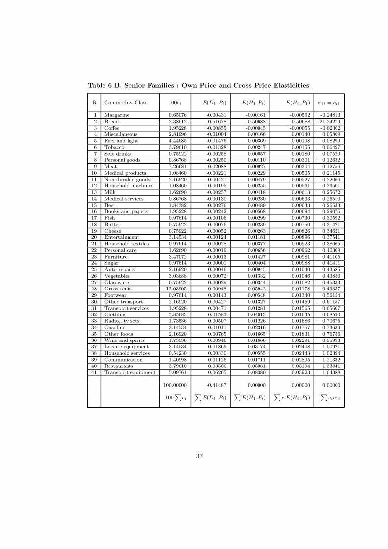
Table 6 B. Senior Families : Own Price and Cross Price Elasticities.

R Commodity Class 100ei E(D1, Pi) E(H1, Pi) E(Hi, P1) σ1i = σi1

1 Margarine 0.65076 -0.00431 -0.00161 -0.00592 -0.248132 Bread 2.38612 -0.51678 -0.50688 -0.50688 -21.242793 Coffee 1.95228 -0.00855 -0.00045 -0.00055 -0.023024 Miscellaneous 2.81996 -0.01004 0.00166 0.00140 0.058695 Fuel and light 4.44685 -0.01476 0.00369 0.00198 0.082996 Tobacco 3.79610 -0.01328 0.00247 0.00155 0.064977 Soft drinks 0.75922 -0.00258 0.00057 0.00180 0.075298 Personal goods 0.86768 -0.00250 0.00110 0.00301 0.126329 Meat 7.26681 -0.02088 0.00927 0.00304 0.12756

10 Medical products 1.08460 -0.00221 0.00229 0.00505 0.2114511 Non-durable goods 2.16920 -0.00421 0.00479 0.00527 0.2206612 Household machines 1.08460 -0.00195 0.00255 0.00561 0.2350113 Milk 1.62690 -0.00257 0.00418 0.00613 0.2567214 Medical services 0.86768 -0.00130 0.00230 0.00633 0.2651015 Beer 1.84382 -0.00276 0.00489 0.00633 0.2653316 Books and papers 1.95228 -0.00242 0.00568 0.00694 0.2907617 Fish 0.97614 -0.00106 0.00299 0.00730 0.3059218 Butter 0.75922 -0.00076 0.00239 0.00750 0.3142119 Cheese 0.75922 -0.00052 0.00263 0.00826 0.3462120 Entertainment 3.14534 -0.00124 0.01181 0.00896 0.3754121 Household textiles 0.97614 -0.00028 0.00377 0.00923 0.3866522 Personal care 1.62690 -0.00019 0.00656 0.00962 0.4030923 Furniture 3.47072 -0.00013 0.01427 0.00981 0.4110524 Sugar 0.97614 -0.00001 0.00404 0.00988 0.4141125 Auto repairs 2.16920 0.00046 0.00945 0.01040 0.4358526 Vegetables 3.03688 0.00072 0.01332 0.01046 0.4385027 Glassware 0.75922 0.00029 0.00344 0.01082 0.4533328 Gross rents 12.03905 0.00948 0.05942 0.01178 0.4935729 Footwear 0.97614 0.00143 0.00548 0.01340 0.5615430 Other transport 2.16920 0.00427 0.01327 0.01459 0.6115731 Transport services 1.95228 0.00471 0.01281 0.01565 0.6560732 Clothing 5.85683 0.01583 0.04013 0.01635 0.6852033 Radio,, tv sets 1.73536 0.00507 0.01226 0.01686 0.7067534 Gasoline 3.14534 0.01011 0.02316 0.01757 0.7363935 Other foods 2.16920 0.00765 0.01665 0.01831 0.7675636 Wine and spirits 1.73536 0.00946 0.01666 0.02291 0.9599337 Leisure equipment 3.14534 0.01869 0.03174 0.02408 1.0092138 Household services 0.54230 0.00330 0.00555 0.02443 1.0239439 Communication 1.40998 0.01126 0.01711 0.02895 1.2133240 Restaurants 3.79610 0.03506 0.05081 0.03194 1.3384141 Transport equipment 5.09761 0.06265 0.08380 0.03923 1.64388

100.00000 -0.41487 0.00000 0.00000 0.00000

100∑

ei

∑

E(D1, Pi)∑

E(H1, Pi)∑

eiE(Hi, P1)∑

eiσ1i

37

8. Final Comments

To summarize, the expenditure system of the CDES indirect utility function:

38

Appendix A. The Box-Cox transformation of a variable

In mathematics, the Box-Cox transformation of a variable x is defined as:

x(λ) =xλ − 1

λ(102)

If λ = 1, then (apart from the constant -1) the variable is linear.If λ → 0, the limits of the numerator and the denominator are equal to zero.Hence we apply de l’Hopital’s rule. We first take the derivative of numeratorand denominator with respect to λ, and take the limit again:

limλ→0

xλ − 1

λ= lim

λ→0

xλ log(x)

1= log(x) (103)

where log denotes the natural logarithm.In econometrics, the Box-Cox transformation is used when we wish to esti-

mate a model, but we are not sure, whether the variables should be included, orwhether their logarithms should be used. The model is estimated in the form ofthe Box-Cox transformation, and it is tested, whether the parameter λ is equalto one, corresponding to the inclusion of the variables, or whether λ is equal tozero, in which case the logarithm of the variables should be used; see Heij et.al. (2005, pp. 297-301) for more details.

In the context of economic theory, the Box-Cox transformation can alsoadvantageously be used in the definition of the indirect utility function of theCDES specification and associated expenditure systems:

V (P, C) =

N∑

i=1

αi(C/Pi)

βi − 1

βi(104)

If βi = 0, then the term, (C/Pi)βi−1

βi, has to be replaced by : log(C/Pi).

If all βi = 0, then CDES (104) can be reduced to,

V (P, C) =

N∑

i=1

αi log(C/Pi) (105)

i.e., to the indirect utility function of the Cobb-Douglas transform.If all βi = σ − 1, then CDES (104) becomes the CES indirect utility function,

V (P, C) =

[

N∑

i=1

αi (C/Pi)σ−1

]

1

σ−1

(106)

In practice, when the CDES model (104) is econometrically estimated, the event- that an estimated coefficient, βi, is zero - is not impossible, but occurs with aprobability of measure zero. That is why (105) is not treated in our main text.

In our exposition, we mentioned the result of Van Driel (1974) and of VanDaal (1982) that at most one βi-parameter is allowed to be: −1. It means thatfor this particular commodity the corresponding term in the indirect utilityfunction should be replaced by : (C/Pi)

−1. But in practice, this special case isagain not impossible, but the probability of occurrence is of measure zero.

39

Appendix B. Derivation of Marshallian demand derivatives

Derivation of the Marshallian demand relation (16) with respect to C gives,

∂Di

∂C=

∂αi(C/Pi)βi+1/∂C

∑

αj(C/Pj)βj−

αi(C/Pi)βi+1∂

(∑

αj(C/Pj)βj /∂C

)

[∑

αk(C/Pk)βk ]2

= (1 + βi)Di

C− Di

∂(∑

αj(C/Pj)βj /∂C

)

∑

αk(C/Pk)βk

= (1 + βi)Di

C−

Di

C

∑

βjej = (1 + βi − β)Di

C(107)

where use has been made of (16), (18), (19). Hence (107) establishes (20).Regarding price derivatives, we first consider the case, i 6= j. Then, Pj

only appears in the denominator, and the derivative of (16) with respect to Pj

becomes [similar result with interchanging the index (i) and (j)],

∂Di

∂Pj= αi(C/Pi)

βi+1 ∂(∑

αk(C/Pk)βk)−1

∂Pj

= −αi(C/Pi)

βi+1

∑

αk(C/Pk)βk×

∂(

αj(C/Pj)βj

)

/∂Pj∑

αk(C/Pk)βk= βj

(

DiDj

C

)

(108)

Secondly, we consider the case, i = j. Then, the term Pi appears in the numer-ator as well as in the denominator of (16). Derivation with respect to Pi gives,after reduction,

∂Di

∂Pi=

∂(

αi(C/Pi)βi+1

)

/∂Pi∑

αk(C/Pk)βk+ βi

(Di)2

C= −(1 + βi)

Di

Pi+ βi

(Di)2

C(109)

Hence (108) and (109) establish (21).Regarding the proof of the derivative (25) of β, (19), we have

∂β

∂C=

∑ ∂ej

∂Cβj =

∑ ∂(PjDjC−1)

∂C=

∑

[

PjC−1 ∂Dj

∂C− C−2PjDj

]

βj

= C−1∑

[

Pj∂Dj

∂C− ej

]

βj (110)

The last expression can, using (107), be rewritten as:

C−1∑

ej(βj − β)βj = C−1∑

ej(βj − β)2 > 0 (111)

where the latter equality is obtained using:∑

ej(βj − β) = 0. Hence (111)establishes (25).

As to the price derivative of β, (19), we get, using (108) and (109):

∂β

∂Pj=

∑

i

βi∂ei

∂Pj

40

=∑

i

βi∂(PiDi/C)

∂Pj=

Djβj

C+

∑

i

Piβi

C

[

βjDiDj

C− (1 + βi)

Di

Piδij

]

= −Djβ

2j

C+

Djβj

C

∑

i

PiDi

Cβi = −βj (βj − β)

Dj

C(112)

Hence (112) establishes (26). From (112) we next obtain:

∂β

∂ lnPj= Pj

∂β

∂Pj= −βj (βj − β)ej (113)

Dedication. This paper is dedicated to: Professor W.H. Somermeyer, Di-rector of the Econometric Institute from 1966 until his untimely death on 31May 1982; visiting professor at the Copenhagen Business School, Fall 1979.

Acknowledgement.

41

References

[1] Allen, R. G. D. (1936), Professor Slutsky’s theory of consumer’s choice,Review of Economic Studies, 3, 120-129.

[2] Allen, R. G. D. and A.L. Bowley (1935),Family Expenditure, P.S. King &Son, London.

[3] Allen, R. G. D. (1950), The Substitution Effect in Value Theory, EconomicJournal, 60, 675-685.

[4] Arrow, K. J. (1961), Additive logarithmic demand functions and the Slut-sky relations, Review of Economic Studies, 28, 176-181.

[5] Arrow, K.J., H.B. Chenery, B. Minhas, R.M. Solow (1961), Capital-laborsubstitution and economic efficiency, Review of Economics and Statistics,42, 225-250.

[6] Arrow, K.J. and M.D. Intriligator (1982), ed. Handbook of MathematicalEconomics, Vol.2, North-Holland, Amsterdam.

[7] Barnett, W. A. (1979), Theoretical Foundations for the Rotterdam Model,Review of Economic Studies, 46, 109-130.

[8] Barten, A.P. (1967), Evidence on the Slutsky Conditions of Demand Equa-tions, Review of Economics and Statistics, 49, 77-84.

[9] Barten, A.P. (1968), Estimating Demand Equations, Econometrica, 36,213-251.

[10] Barten, A.P. (1969), Maximum Likelihood Estimation of a Complete Sys-tem of Demand Equations, European Economic Review, 1, 7-73.

[11] Barten, A.P. and E. Geyskens (1974), The Negativity Condition in Con-sumer Demand, European Economic Review, 6, 227-260.

[12] Barten, A.P. (1977), The System of Consumer Demand Functions Ap-proach: A Review, Econometrica, 45, 23-51.

[13] Barten, A.P. and V. Boehm (1982), Consumer Theory, Chapter 9, in Arrowand Intriligator (1982).

[14] Cobb, C.W. and P.H. Douglas (1928), A theory of production, AmericanEconomic Review, Papers and Proceedings, XVIII, 139-165.

[15] Chung, J.W. (1994), Utility and Production Functions, Blackwell, Oxford.

[16] Cramer, J.S. (1970), Interaction of price and income in consumer demand,European Economic Review, 1, 428-436.

[17] Deaton, A.S. (1974), A reconsideration of the empirical implications ofadditive preferences, Economic Journal, 84, 338-348.

42

[18] Deaton, A.S. (1975), The Measurement of Income and Price Elasticities,European Economic Review, 6, 261-273.

[19] Deaton, A.S. and J. Muellbauer (1980a), Economics and Consumer Behav-ior, Cambridge University Press, Cambridge.

[20] Deaton, A.S. and J. Muellbauer (1980b), An Almost Ideal Demand System,American Economic Review, 70, 312-326.

[21] De Boer, P.M.C. and M. Missaglia (2005), Introducing the Indirect Ad-dilog System in a Computable General Equilibrium Model: a Case Studyfor Palestine, Report EI 2005-25 of the Econometric Institute, ErasmusUniversity Rotterdam, the Netherlands.

[22] Diewert, W.D. (1974), Applications of Duality Theory, Chapter 3, in In-triligator and Kendrick (1974).

[23] Diewert, W.D. (1982), Duality Approaches to Microeconomic Theory,Chapter 12, in Arrow and Intriligator (1982).

[24] Engel, E. (1857), Die Productions- and Consumptionsverhaeltnisse desKoenigreichs Sachsen, Zeitschrift des Statistischen Bureaus des KoeniglichSaechsishen Ministerium des Inneren, No. 8-9, Sonntag, November 22,1857; reprint, Bulletin of the International Statistical Institute,(1895), 9,1-54.

[25] Engel, E. (1895), Die Lebenshaltung belgischer Arbeiterfamilien frueherand jetzt, Bulletin of the International Statistical Institute, 9, 1-124, withan Appendix, 1-54.

[26] Frisch, R. (1959), A Complete Scheme for Computing All Direct and CrossDemand Elasticities in a Model with Many Sectors, Econometrica, 27, 177-196.

[27] Fuss, M. and D. McFadden (1978), ed. Production Economics: A DualApproach to Theory and Applications, Vol.1, North-Holland, Amsterdam.

[28] Geary, R.C. (1949-1950), A Note on a Constant Utility Index of the Costof Living, Review of Economic Studies, 18, 65-66.

[29] Goldberger, A.S. (1970), A Cross-Country of Consumer Expenditure Pat-terns, European Economic Review, 2, 357-400.

[30] Hanoch, G. (1971), CRESH Production Functions, Econometrica, 39, 695-712.

[31] Hanoch, G. (1975), Production and Demand Models with Direct and Indi-rect Implicit Additivity, Econometrica, 43, 395-419.

[32] Hanoch, G. (1978), Polar Functions with Constant Two Factors - One PriceElasticities, Chapter II.3, in Fuss and McFadden (1978).

43

[33] Heij, C., P.M.C. de Boer, P.H. Franses, T.Kloek and H.K. van Dijk (2004),Econometric Methods with Applications in Business and Economics, Ox-ford University Press, Oxford.

[34] Hicks, J.R. and R.G.D. Allen (1934), A Reconsideration of the Theory ofValue. Part I-II, Economica, 1, 52-57, 196-219.

[35] Hicks, J.R. (1969), Direct and Indirect Additivity, Econometrica, 37, 353-354.

[36] Houthakker, H.S. (1952), Compensated Changes in Quantities and Quali-ties Consumed, Review of Economic Studies, 19, 155-64.

[37] Houthakker, H.S. (1957), An International Comparison of Household Ex-penditure Patterns Commemorating the Centenary of Engel’s Law , Econo-metrica, 25, 532-51.

[38] Houthakker, H.S. (1960), Additive Preferences, Econometrica, 28, 244-257.

[39] Houthakker, H.S. (1965), A Note on Self-Dual Preferences, Econometrica,33, 797-801.

[40] Houthakker, H.S. (1965), New Evidence on Demand Elasticities, Econo-metrica, 33, 277-288.

[41] Intriligator, M.D. and D.A. Kendrick (1974), ed., Frontiers of QuantitativeEconomics, Vol.2, North-Holland, Amsterdam.

[42] Jensen, B.S. (1980),Expenditure System for the Danish Household Sector,Symposium i Annvendt Statistik, NEUCC, Lyngby, Denmark, 263-296.

[43] Jensen, B.S. and M. E. Larsen (2005), General Equilibrium Dynamics ofMulti-Sector Growth Models, Journal of Economics, Suppl. 10, 17-56.

[44] Joergensen, E. (1965), Income-Expenditure Relations of Danish Wage andSalary Earners, Statistical Inquires No. 14, Statistical Department, Copen-hagen.

[45] Katzner, D.W. (1968), A Note on the Differentiability of Consumer De-mand Equations, Econometrica, 36, 415-418.

[46] Klein, L.R. and H. Rubin (1948-1949), A Constant-Utility Index of theCost of Living, Review of Economic Studies, 15, 84-87.

[47] Kloek, T. and H. Theil (1965), International Comparisons of Prices andQuantities Consumed, Econometrica, 33, 535-556.

[48] Kreps, D.M. (1995), A Course in Microeconomic Theory, Harvester Wheat-sheaf, New York.

[49] Leser, C.E.V. (1941), Family Budget Data and Price-Elasticities of De-mand, Review of Economic Studies, 9, 40-57.

44

[50] Leser, C.E.V. (1964), Forms of Engel curves, Econometrica, 32, 443.

[51] Lluch, C. and A. Powell (1975), International Comparisons of ExpenditurePatterns, European Economic Review, 5, 275-303.

[52] Marschak, J. (1943), Demand Elasticities Reviewed, Econometrica, 11, 25-34.

[53] Mas-Colell, A., M.D. Whinston and J.R. Green (1995), Microeconomic The-ory, Oxford University Press, New York.

[54] Marshall, A. (1920), Principles of Economics, 8.ed., Macmillan, London.

[55] Mukerji, V. (1963), A Generalized SMAC Function with Constant Ratiosof Elasticity of Substitution, Review of Economic Studies, 30, 233-236.

[56] Parks, R.W. (1969), System of Demand Equations: An Empirical Compar-ison of Alternative Functional Forms, Econometrica, 37, 629-650.

[57] Pollak, R.A. and T.J. Wales (1969), Estimation of the Linear ExpenditureSystem, Econometrica, 37, 611-628.

[58] Pollak, R.A. (1972), Generalized Separability, Econometrica, 40, 431-453.

[59] Prais, J.S and H. S. Houthakker (1971), Analysis of Family Budgets, 2.ed,Cambridge University Presss, London.

[60] Roy, R. (1947), La Distribution du Revenue entre les Divers Biens, Econo-metrica, 15, 205-225.

[61] Sato, K. (1972), Additive Utility Functions with Double-Log Demand Func-tions, Journal of Political Economy, 80, 102-124.

[62] Samuelson, P.A. (1948), Some Implications of Linearity, Review of Eco-nomic Studies, 30, 88-90.

[63] Samuelson, P.A. (1950), The Problem of Integrability in Utility Theory,Economica, 17, 355-385.

[64] Samuelson, P.A. (1965), Using Full Duality to Show that SimultaneouslyAdditive Direct and Indirect Utilities implies Unitary Price Elasticity ofDemand, Econometrica, 33, 781-796.

[65] Samuelson, P.A. (1969), Corrected Formulation of Direct and Indirect Ad-ditivity, Econometrica, 37, 355-359.

[66] Silberberg, E. and W. Suen (2001), The Structure of Economics, A Math-ematical Analysis, 3. edition, McGraw-Hill, Singapore.

[67] Smith, Adam (Edwin Cannan, 6.ed.), The Wealth of Nations, Vol. 1,Methuen, London, 1961.

45

[68] Somermeyer, W.H. and J.W.W.A. Wit (1956), Een Verdeelmodel (an Al-location Model), Report M14, Statistics Netherlands, Voorburg.

[69] Somermeyer, W.H. and A. Langhout (1972), Shapes of Engel Curves andDemand Curves: Implications of the Expenditure Model, Applied to DutchData, European Economic Review, 3, 351-386.

[70] Stone, R. (1954), Linear Expenditure System and Demand Analysis: anApplication to the British Pattern of Demand, Economic Journal, 64, 511-532.

[71] SU, Nr. 34 (1977), Oekonomiske Forhold i Loenmodtagerhusstande: For-brugsundersoegelsen 1971, Danmarks Statistik, Koebenhavn.

[72] Theil, H. (1965), The Information Approach to Demand Analysis, Econo-metrica, 33, 67-87.

[73] Tinbergen, J. (1942), Professor Douglas’ Production Function, Revue del’Institut International de Statistique, 10, 37-48.

[74] Van Daal, J. (1983), On the Utility Functions of the Indirect Addilog Bud-get Allocation Model, Report 8304, Econometric Institute, Erasmus Uni-versity Rotterdam, The Netherlands.

[75] Van Driel, J. (1974), Consumer Expenditure Allocation Models, Report7405, Econometric Institute, Erasmus University Rotterdam, The Nether-lands.

[76] Varian, H.R. (1992), Microeconomic Analysis, 3. edition, Norton, NewYork.

[77] Wit, J.W.W.A. (1957), Inkomenselasticiteiten in 1935/’36 and 1951 voorNederland: Toepassing van een Model van Inkomensbesteding, Statistischeen Econometrische Onderzoekingen, Statistics Netherlands, Voorburg, 27-41.

[78] Wit, J.W.W.A. (1960), Income Elasticities in 1935/’36 and 1951 in theNetherlands: an Application of a Model for Income Spending, StatisticalStudies, Vol. 10, Statistics Netherlands, Voorburg.

[79] Wold, H. (1940), Efterfrgan p Jordbruksprodukter och dets Kaenslighet forPris- og Indkomstforaendringer, S.O.U.: 16, Stockholm.

[80] Wold, H. (1952), Demand Analysis, John Wiley & Sons, New York.

[81] Wold, H. (1970), Giffen‘s Paradox and the Marshallian Demand Curve,The Manchester School, 38, 65-71.

46

Addresses of authors: Bjarne S. Jensen, Department of Economics, Copen-hagen Business School, Solbjerg Plads 3, DK-2000 Frederiksberg, Denmark,e-mail: bsj.eco@cbs.dk - Paul de Boer, Department of Econometrics, ErasmusUniversity Rotterdam, P.O. Box 1738, NL-3000 DR Rotterdam, The Nether-lands, e-mail: pmdeboer@few.eur.nl.

47