Embed Size (px)
Citation preview
ANNALS OF PHYSICS 144, 81-106 (1982)
The Structure of the Space of Solutions of Einstein’s Equations II:
Several Killing Fields and the Einstein-Yang-Mills Equations
JUDITH M. ARMS
Department of Mathematics, University of Washington, Seattle, Washington 98195
JERROLD E. MARSDEN
Department of Mathematics, Universit.v of California, Berkeley, Calgornia 94720
AND
VINCENT MONCRIEF
Department of Physics, Yale Universitv, P.O. Box 6666, New Haven, Connecticut 065/I
Received April 27, 1982
The space of solutions of Einstein’s vacuum equations is shown to have conical singularities
at each spacetime possessing a compact Cauchy surface of constant mean curvature and a nontrivial set of Killing fields. Similar results are shown for the coupled Einstein-Yang-Mills
system. Combined with an appropriate slice theorem, the- results show that the space of geometrically equivalent solutions is a stratified manifold with each stratum being a symplectic manifold characterized by the symmetry type of its members.
Contents. Introduction. 1. The Kuranishi map and its properties. 2. The momentum constraints. 3. The Hamiltonian constraints. 4. The Einstein-Yang-Mills system. 5.
Discussion and examples.
This paper is the second part of Fischer et al. (1980) and is a companion of Arms et al. (19:81). In Fischer et al. (1980) we studied the space &? of solutions to Einstein’s vacuum equations near a spacetime (V, (4’g,) which has a compact Cauchy surface of constant mean curvature and with k = k(‘4’g,) = (dim of the space of Killing fiellds of “‘g,) = 1. Here we study the case k > 1 and extend the results to the coupled Einstein-Yang-Mills equations by utilizing the present methods together with known results for the pure Yang-Mills case from Moncrief (1977) and Arms (1981). In Arms el’ al. (1981) it was shown how to deal with the case k > 1 in case all the Killing fields are spacelike. The present paper builds on these techniques.
81 0003.4916/82/130081-26$05.00/O
Copyright C 1982 by Academic Press. Inc. All nghfs of reproductmn in any form reserved.
82 ARMS,MARSDEN,ANDMONCRIEF
If k = 0, i.e., (4)g,, has only trivial Killing fields, then it has been known for some time that B is a smooth manifold near (4)g0. This was established in the period 1973- 1975 through the work of Fischer, Marsden and Moncrief-see Fischer et al. (1980) for references. The analogous results for the pure Yang-Mills equations are due to Moncrief (1977) and, for the Einstein-Yang-Mills equations, to Arms (1979). Combined with an appropriate slice theorem (see Fischer et al. (1980), Isenberg and Marsden (1982) and references therein) and the reduction methods of Marsden and Weinstein (1974), one sees that B/(gauge transformations) is a smooth symplectic manifold near such “‘g,. For k 2 1, which is usually regarded as the most interesting case, g is no longer smooth and so B/(gauge transformations) is considerably more complicated. In fact, it becomes a stratified symplectic manifold, as is explained in .Isenberg and Marsden (1982).
Briefly, Fischer et al. (1980) proved that for k = 1, B has a conical singularity at (4)g0; i.e., near “)g,, B can be written in a suitable chart as the zero set of a homogeneous quadratic function. The generators of this cone consist of those symmetric two tensors (4)h such that
(9 (4)h satisfies the linearized Einstein equations
D Ein(‘4’g,) . (4)h = 0,
where Ein(‘4’g) is the Einstein tensor formed from a metric (4’g and D denotes the Frechet derivative and
(ii) the Taub conserved quantities vanish:
I (4)X. [D2 Ein(‘4’g,) . ((4’h, (4)h)] . (4)2Z d3Z = 0, z
where ‘4)X is a Killing field for (4)g0, C is a compact Cauchy surface and (4’Zz is its forward pointing unit normal.
It follows that a necessary and suflcient condition for a solution (4’h of the linearized equations to be tangent to a curve of solutions to Einstein’s equations passing through (4’g0 is that (ii) holds.
The principal result of this paper is
THEOREM. The preceding statement for k(‘4’g,) = 1 also holds for k(‘4’g,) > 1 and similar results hold for the Einstein-Yang-Mills system.
The precise function spaces employed in this theorem were detailed in Fischer et al. (1980) and will be assumed implicitly here.
The case k(‘4’g,) > 1 includes more interesting examples than the case k(‘4’g,) = 1. In particular, it includes the flat spacetime T3 x R (with k = 4) which was the example which began the subject in the seminal paper of Brill and Deser (1973).
The proof of the above theorem occupies Sections l-3 of the paper. A crucial tool
EINSTEIN’S EQUATIONS 83
required for k > 1 that was not needed for k = 1 is the “Kuranishi map,” a mapping that was used originally by Kuranishi (1965) in studies of deformations of complex structures and applied by Atiyah et al. (1978) to the study of Euclidean Yang-Mills fields. As was shown by Arms et al. (198 l), this technique may be used to prove the theorem in the case all the Killing fields are spacelike. The general plan of our proof in the general case is to combine the Kuranishi approach, which is able to deal with all the momentum constraints and a certain projection of the Hamiltonian constraint, with a special Morse lemma-type argument for the Hamiltonian constraint.
Section 1 reviews the definition and some basic properties of the Kuranishi map. In particular, we see that this map (restricted to a slice) is symplectic and that its inverse was implicitly defined in Fischer et al. (1980).
Section 2 shows that the Kuranishi map enables one to solve all of the momentum constraints and Section 3 then shows how to subsequently solve the Hamiltonian constraint by a special argument. This last step relies on a suitable infinite dimen- sional Morse lemma due to Tromba (1976) and Golubitsky and Marsden (1982).
Section 4 extends the results to the Einstein-Yang-Mills system, the Einstein- Maxwell system being a special case. There is a peculiar difficulty posed by this system. Namely, with the set up most natural from the bundle viewpoint, the super- momentum constraint is a cubic function of the fields, a situation which causes havoc with the Kuranishi method. This difficulty is overcome by a special parametrization of the shift and gauge shift (X, v), which, in effect, transforms the constraint to an equivalent quadratic one. When this is done, the methods proceed in a way similar to the vacuum case.
The final section discusses the singularities and how symmetry is broken by means of a collection of remarks and examples. The relationship to the work of Jantzen (1979) is briefly mentioned. Finally, a mechanism for symplectically desingularizing the solution space is discussed.
From our work in Fischer et al. (1980), it’ is enough to study the constraint equations. We now recall some of the notation that will be used in this connection. The reader should consult Fischer et al. (1980) for additional explanation and details.
Let M be a compact 3-manifold and A the space of (Ws,P, s > 3/p + 1) Riemanni,an metrics on M and let P = T*_X denote the “natural” cotangent bundle of L1; i.e., t.he fiber of T*A over g E M consists of all symmetric 2-contravariant tensor densities x (of class IV-‘~“). The constraint set of the vacuum Einstein equations on a 4-dimensional spacetime in which M is embedded as a compact hyper- surface, is the set
GF = V’(O),
where @: T*A* (densities on M) x (one-form densities on M) is defined by @(g, 7~) = (Z( g, 7c), f( g, x)) and X and / are given by
R(g, n> = iv . n’ - +(trace z’)*) --R(g)}p(g)
84 ARMS, MARSDEN, AND MONCRIEF
and
.P(g, 7c)i = -27ci’,j.
Here 7c = rc’ 0 p(g), ,u( g) is the volume form of g, and R(g) is the scalar curvature of g.
The vacuum Einstein equations for a metric (4)g are equivalent to the constraint equations @(g, n) = 0 for the induced Cauchy data (g, rc) on a hypersurface C and the evolution equations
a g ( 1 = -J 0 D@(g, 7r)*
N
at n ( 1 x
relative to a given spacetime slicing. Here J is the (almost) complex structure on T*-X given by
Ib 0 --
J= i ! P(g)
e4g) 0
where Ib and r# are the index lowering and raising operators relative to g. The adjoint D@(g, n)* is taken relative to the L* metric on T*.M given by
In this formula, . denotes contraction using the base point g and the natural pairing between (densities) x (one-form densities) and (functions) x (vector fields). Thus D@( g, n)*: (functions x vector fields) -+ Ttg,nj(T*M), and one can compute it explicitly. (See Fischer et al. (1980) for the formula.)
The (weak) symplectic structure on T*A is given by
which is independent of (g, rr). Note that .J2 = -1, 31 is symplectic, and is orthogonal and skew adjoint with respect to ((, )).
The Killing fields of (4)g are in one-to-one correspondence with elements of ker D@( g, rc)* by means of perpendicular and parallel projection: X+ (Xi, X,,).
The following fundamental decomposition of Moncrief (1975) will be used (Fischer et al., 1980, Theorem 2.5):
T,,,,,(T*A) = range(-J o D@(g, n)*) @ range(D@(g, rc)*)
0 [ker(D@( g, n) 0 J) n ker D@( g, z)]. W
EINSTEIN’S EQUATIONS 85
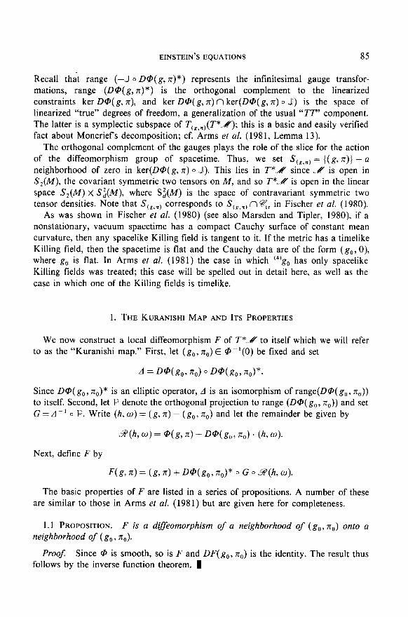
Recall that range (-J o D@(g, x)*) represents the infinitesimal gauge transfor- mations, range (D@(g, n)*) is the orthogonal complement to the linearized constraints ker D@( g, n), and ker D@( g, Z) n ker(D@( g, X) 0 JJ) is the space of linearized “true” degrees of freedom, a generalization of the usual “TT” component. The latter is a symplectic subspace of Tcg,=, (T*M); this is a basic and easily verified fact about Moncrief s decomposition: cf. Arms et al. (198 1, Lemma 13).
The orthogonal complement of the gauges plays the role of the slice for the action of the diffeomorphism group of spacetime. Thus, we set ScRqx) = {(g, rc)} + a neighborhood of zero in ker(D@(g, n) o JJ). This lies in T*M since _H is open in S,(M), the covariant symmetric two tensors on M, and so T*..H is open in the linear space S,(IM) x S:(M), where S:(M) is the space of contravariant symmetric two tensor densities. Note that ScglR) corresponds to Scp,R) n U;;, in Fischer et al. (1980).
As was shown in Fischer et af. (1980) ( see also Marsden and Tipler, 1980) if a nonstation,ary, vacuum spacetime has a compact Cauchy surface of constant mean curvature, then any spacelike Killing field is tangent to it. If the metric has a timelike Killing field, then the spacetime is flat and the Cauchy data are of the form (g,, 0), where g, is flat. In Arms et al. (198 1) the case in which (4)g0 has only spacelike Killing fields was treated; this case will be spelled out in detail here, as well as the case in which one of the Killing fields is timelike.
1. THE KURANISHI MAP AND ITS PROPERTIES
We now construct a local diffeomorphism F of T*M to itself which we will refer to as the “Kuranishi map.” First, let (g,, q,) E V’(O) be fixed and set
A = D@(g,, no) 0 D@(g,, no>*.
Since D@( g,, q-J* is an elliptic operator, A is an isomorphism of range(D@( g,, x0)) to itself. Second, let P denote the orthogonal projection to range (D@( g,, n,,)) and set G = A-’ o P. Write (h, o) = (g, X) - (g,, n,) and let the remainder be given by
.R(h, 0) = @(g, n> -@q&J, 710) . (h, w).
Next, define F by
F(g, n> = (g, n) + D@(g,, q,>* 0 G 0 9th co>.
The basic properties of F are listed in a series of propositions. A number of these are similar to those in Arms et al. (1981) but are given here for completeness.
1.1 PROPOSITION. F is a d@eomorphism of a neighborhood of (g,, q,) onto a neighborhood of (g,, q).
ProoJ: Since @ is smooth, so is F and DF(g,, q) is the identity. The result thus follows by the inverse function theorem. 1
86 ARMS,MARSDEN,AND MONCRIEF
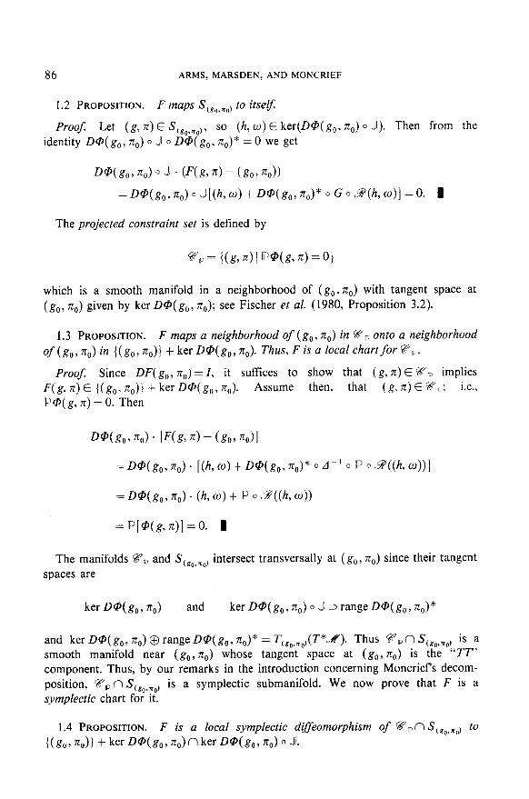
1.2 PROPOSITION. F maps S~no,no~ to itself.
Proof: Let (g, n> E ScgO,ROJ, so (h, o) E ker(D@( g,, q,) 0 JJ). Then from the identity D@( g,, rcO) 0 J o D@( g,, rrO) * = 0 we get
m(g,,,q,)oJ . (F(g,~)-(g,,%>) = mqg,, TC,,) 0 JJ[(~, w) + m(g,, q,)* 0 G 0 s(k ~11 = 0. 1
The projected constraint set is defined by
which is a smooth manifold in a neighborhood of (g,, q,) with tangent space at (g,, rr,,) given by ker D@( g,, z,,); see Fischer et al. (1980, Proposition 3.2).
1.3 PROPOSITION. F maps a neighborhood of (g,, x0) in q Ip onto a neighborhood of (g,, q,) in ((g,, n,,)} + ker D@( g,, q,). Thus, F is a local chart for gp.
ProojI Since DF(g,, x0) = I, it suffices to show that (g, rz) E gp implies F( g, n) E ((g,, n,)) + ker D@( g,, q,). Assume then, that (g, n) E gV: i.e., Ip@( g. n) = 0. Then
D@(g,, no> . [f’(g, 7~) - (go, no>]
= m( g,, no) e (h, w) + p 0 .g((h, W))
=lP[@(g,7r)]=O. I
The mamfoids G?3ip and SCgO+,) intersect transversally at (g,, z,,) since their tangent spaces are
ker D@(g,, no) and ker D@(g,, q,) 0 J 1 range D@(g,, n,>*
and ker D@( g,, rc,,) @ range D@( g,, n,)* = TC,,,,,,(T*y/Y). Thus E’,n SCp,,+,) is a smooth manifold near (g,, q,) whose tangent space at (g,, rr,,) is the “TT’ component. Thus, by our remarks in the introduction concerning Moncriefs decom- position, g71p n SCgO,xOj is a symplectic submanifold. We now prove that F is a symplectic chart for it.
1.4 PROPOSITION. F is a local symplectic dSffeomorphism of qpn Slno.xa, to {(g,, T,)} + ker D@(g,, q,)n kerD@(g,, F,) 0 JJ.
EINSTEIN’S EQUATIONS 87
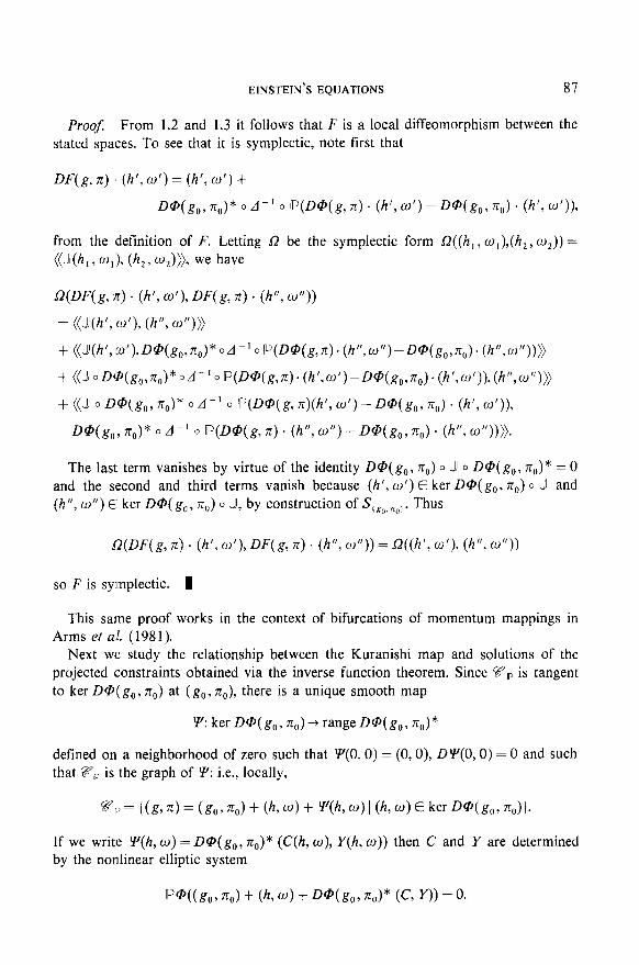
ProoJ From 1.2 and 1.3 it follows that F is a local diffeomorphism between the stated spaces. To see that it is symplectic, note first that
DF( g, n) (h’, w’) = (h’, w’) +
D@(g,, To)* 0 A-’ 0 P(D@( g, 7c) ’ (h’, 0’) - D@( g,, 710) * (II’, w’)),
from the definition of F. Letting R be the symplectic form Q((h,, o,),(h,, wZ)) = ((.W,, q>, (h,, WA)>, we have
Q(DF( g, ;T) . (h’, co’), DF( g, z) . (h”, co”))
= ((J(h’, co’), (h”, u”)})
+ ((Jq’, Ito’ ),D~(g,,~,)*oA-‘~IP(D~(g,n).(h”,w”)-D~(g,,~,)~(h”.w”))))
+ ((JoD@(g,,n,)*oA-‘0 IP(D@(g,n). (h’,o’)-D@(g,,n,). (h’,w’)),(h”,o”)})
+ ((JJ 0 D@(g,, n,,)* 0 A-’ 0 ip(D@( g, n)(h’, w’) - D@(g,, q)) . (A’, OJ’)),
D@(g,, To)* 0 A-’ fJ P(D@( g, 7c) * (h”, 0”) - my g,, 7rJ * (h”, co”)))).
The last term vanishes by virtue of the identity D@( g,, x0) 0 J 0 D@(g,, Q)* = 0 and the slecond and third terms vanish because (h’, w’) E ker D@(g,,, ?‘cO) 0 $ and (h”, w”) E ker D@( g,, 71~) o J, by construction of ScgO,XO). Thus
Q(DF( g, n) . (h’, co’), DF( g, n) . (A”, co”)) = fi((h’, w’), @“, @“)I
so F is sylmplectic. 1
This same proof works in the context of bifurcations of momentum mappings in Arms et al!. (1981).
Next we study the relationship between the Kuranishi map and solutions of the projected constraints obtained via the inverse function theorem. Since qP is tangent to ker D@I(g,, rc,,) at (g,, rcO), there is a unique smooth map
Y:kerD@(g,,n,)-+rangeD@(g,,n,)*
defined on a neighborhood of zero such that Y(0, 0) = (0, 0), D!P(O, 0) = 0 and such that VP is the graph of Iy: i.e., locally,
If we write Y(h, W) = D@(g,, rcJ* (C(h, w), Y(h, 0)) then C and Y are determined by the nonlinear elliptic system
~@((g,, q) + (k w> + D@(g,, %J* (CT Y)) = 0.
88 ARMS,MARSDEN, AND MONCRIEF
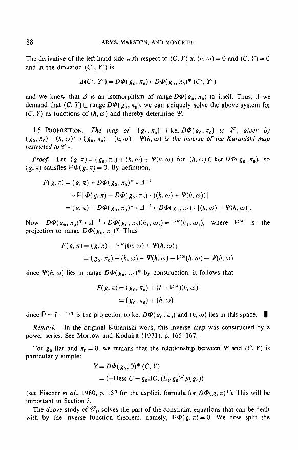
The derivative of the left hand side with respect to (C, Y) at (h, w) = 0 and (C, Y) = 0 and in the direction (C’, Y’) is
d(C’, Y’) = D@(g,, q)) 0 D@(g,, no)* (C’, Y’)
and we know that A is an isomorphism of range D@( g,, rr,,) to itself. Thus, if we demand that (C, Y) E range D@( g,, rcr,), we can uniquely solve the above system for (C, Y) as functions of (h, o) and thereby determine Y.
1.5 PROPOSITION. The map of ((g,,,n,)} + kerD@(g,,n,) to g0 given by (g,, q,) + (h, w) tr (g,, q,) + (h, w) + !P(h, o) is the inverse of the Kuranishi map restricted to VP.
Proof. Let (g, rr) = (g,, rr,,) -t (h, w) + Y’(h, o) for (h, o) E ker D@( g,, n,), so (g, rr) satisfies P@( g, n) = 0. By definition,
F(g,n)=(g,Ir)+D~(g,,n,)*oA~’
0 p[@s(g, n) - Wg,, xi,> . ((k 0) + W, w,,l
= (g, z) - D@(g,, q,)* 0 A-’ 0 D@(g,, T,> . [(h, w) + ‘f’Y(k u)l.
Now D@(g,, no)* 0 A-’ 0 Dc?(g,, q,)(h,, co,)= IP*(h,, CO,), where P* is the projection to range DQi(g,, rrO)*. Thus
F(g,71)=(g,7L)--IP*lth,u)+ y@,w)j
= (go, q,) + (h, u) + Y(h, 0) - p*(h, u) - V, a)
since Y(h, o) lies in range D@(g,, x0)* by construction. It follows that
F(g, r>= (g,,, T,> + (I- p*)(k w)
= (go > 4 + (k w>
since a = I - P* is the projection to ker D@(g,, rr,,) and (h, o) lies in this space. 1
Remark. In the original Kuranishi work, this inverse map was constructed by a power series. See Morrow and Kodaira (1971), p. 165-167.
For g, flat and rr,, = 0, we remark that the relationship between !P and (C, Y) is particularly simple:
y= D@(g,, o)* (C, y>
= (-Hess C - g,AC, 6% gJ#,4g,))
(see Fischer et al., 1980, p. 157 for the explicit formula for D@(g, rr)*). This will be important in Section 3.
The above study of gP solves the part of the constraint equations that can be dealt with by the inverse function theorem, namely, P@(g, 7~) = 0. We now split the
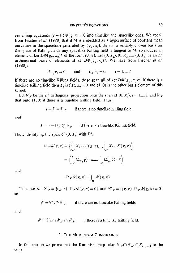
EINSTEIN’S EQUATIONS 89
remaining equations (I- P) @(g, rc) = 0 into timelike and spacelike ones. We recall from Fisch’er et al. (1980) that if A4 is embedded as a hypersurface of constant mean curvature i,n the spacetime generated by (g,, n,), then in a suitably chosen basis for the space of Killing fields any spacelike Killing field is tangent to M, so induces an element of ker D@( g,, n,)* of the form (0, X). Let (0, X,), (0, X,) ,..., (0, X,) be an L2 orthonormal basis of elements of ker D@( g,, x0)*. We have from Fischer et al. (1980):
Lx,kh=O and Q-4) = 0, i = l,.... 1.
If there are no timelike Killing fields, these span all of ker D@(g,, rr,,)*. If there is a timelike Killing field then g, is flat, x,, = 0 and (1,0) is the other basis element of this kernel.
Let P, be the L2 orthogonal projection onto the span of (0, Xi), i = l,..., I, and P, that onto (1,O) if there is a timelike Killing field. Thus,
I-P=lPy if there is no timelike Killing field
and
I-lP=PIp,@P, if there is a timelike Killing field.
Thus, identifying the span of (0, Xi) with R’.
Thus, we set qr= ((g,rc)I P,@(g,n)=O) and gp= {(g,n)I P,@(g,n)=O) so
F=FpnFr if there are no timelike Killing fields
and
F=Fpng,,ng,, if there is a timelike Killing field.
2. THE MOMENTUM CONSTRAINTS
In this section we prove that the Kuranishi map takes &n %? In Scno,zoj to the cone
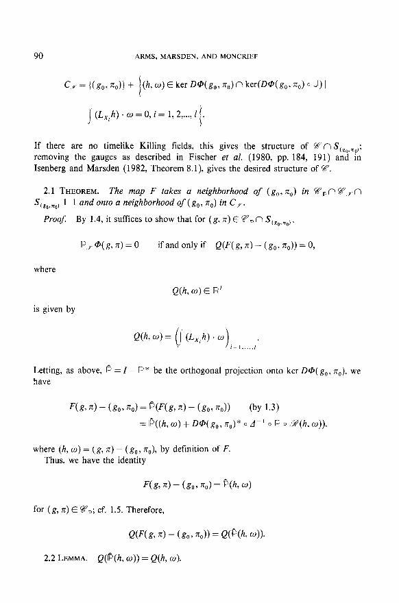
90 ARMS,MARSDEN.AND MONCRIEF
c,={(g,,~Jl+ (h,w)EkerD~(g,,n,)nker(D~(g,,~,)o9)1 I I (L,& . 0 = 0, i = 1, 2 ,..., 1 i .
If there are no timelike Killing fields, this gives the structure of ‘Z n SCgglxO,; removing the gauges as described in Fischer et al. (1980, pp. 184, 19 1) and in Isenberg and Marsden (1982, Theorem 8. l), gives the desired structure of g.
2.1 THEOREM. The map F takes a neighborhood of (g,, n,) in gP n 97 pn S cg,,n,j l-l and onto a neighborhood of (g,, q,) in C,.
Proof: By 1.4. it suffices to show that for (g, n) E g”,n S,Ro,Ro),
~,@(g,~)=o if and only if Q(F( g, z) - (g,, x0)) = 0,
where
is given by
Q(k 0) = 1' (Lx+) - CL) . i=l,..../ Letting, as above, P = I - P * be the orthogonal projection onto ker D@( g,, rr,,), we have
F(g, n) - (go, T,) = &Fk, 7~) - (go, no>> (by 1.3)
= @((h, o) + D@(g,, n,)* 0 A-’ 0 fF o.S?(h, co)).
where (h, w) = (g, 7~) - (g,, Q), by definition of F. Thus, we have the identity
F(g, n>- (go, %I = p(h, 0)
for (g, z) E @n; cf. 1.5. Therefore,
Q(F(g, x>- (go, T,)) = Q(p(k WI>-
2.2 LEMMA. Q(P(h, w)) = Q@, 0).
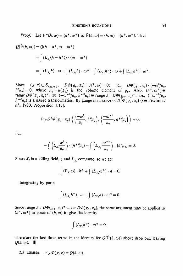
EINSTEIN'S EQUATIONS
Proof Let P*(h, o) = (h*, w*) so p(h, w) = (h, o) - (h*, w*). Thus
91
Q(&h, o)) = Q(h -A*, w - co*)
= ( (L,Jh - II*)) * (w - w*>
= 1 (L,,h) * 0 - I’ (L,;h) . co* -J (L,jz*). w +I (L&z”) * w*.
Since (g! n> E ~~ga,no~, D@(g,, 7cJ 0 J(h, 0) = 0; i.e., D@(g,, no). (--d/p,. h#p,) = 0. where ,q, = p( g,) is the volume element of g,. Also, (h*, CD*) E rangeD@(,p,, 74J*, so (-w*~/P~, h*#p,) E range J 0 D@(g,, q)*; i.e., (-u*“/p,, h*#& is a gauge transformation. By gauge invariance of D*@( g,, rr,,) (see Fischer et al., 1980, Proposition 1.12),
i.e.,
Since Xi is a killing field, b and Lxi commute, so we get
J (LXi4. h* + )'(Lp*)* h=O.
Integrating by parts,
I'(Lx,h*)* w+ I‘(Lxih)*w*4
Since range J 0 D@( g,, q,)* c ker D@( g,, q,), the same argument may be applied to (h*, o*) in place of (h, W) to give the identity
j‘(Lxih*) * w* = 0.
Therefore the last three terms in the identity for Q(P(h, o)) above drop out, leaving Q(k ~1. I
2.3 LEMMA. p, @(g, 7~) = Q(k 0).
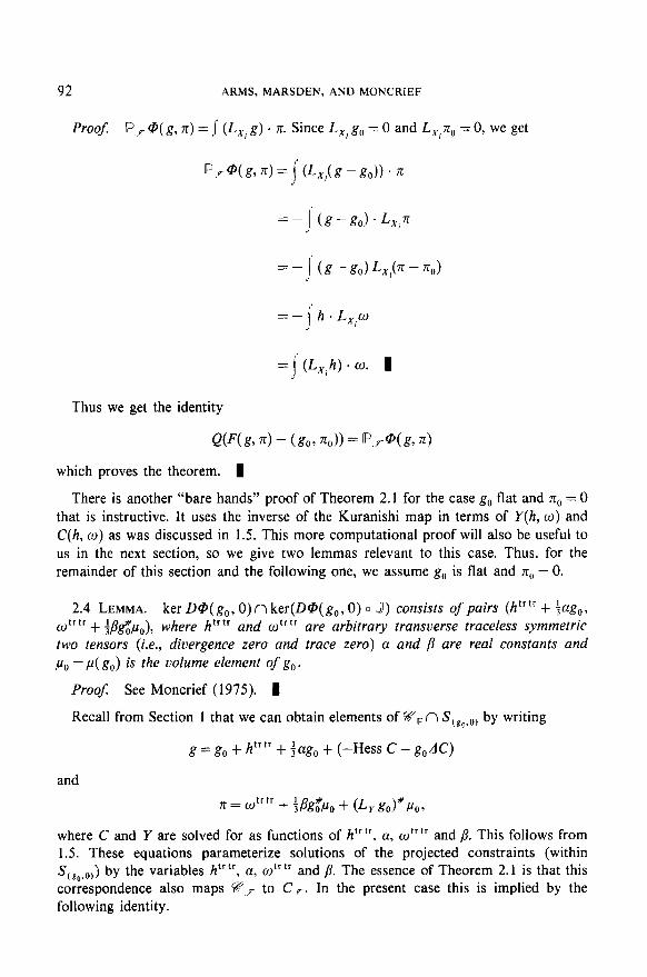
92 ARMS,MARSDEN,AND MONCRIEF
Proof: ~,@(g, r) = I Lid * z Since LXi g, = 0 and Lxin, = 0, we get
b @‘(g7 xl = j v& - &I)) . 71
=- &g,)*L,in !
xz- i
h . Lxiw
= I‘ (Lxih) - w. 1
Thus we get the identity
QF(g> n> - (go, d) = ‘?,@(g, n>
which proves the theorem. 1
There is another “bare hands” proof of Theorem 2.1 for the case g, flat and rcO = 0 that is instructive. It uses the inverse of the Kuranishi map in terms of Y(h, o) and C(h, w) as was discussed in 1.5. This more computational proof will also be useful to us in the next section, so we give two lemmas relevant to this case. Thus, for the remainder of this section and the following one, we assume g, is flat and x0 = 0.
2.4 LEMMA. ker D@(g,, O)f? ker(D@(g,, 0) o JJ) consists of pairs (htrtr + fag,, cotrtr + $g&,), where h”” and co”” are arbitrary transverse traceless symmetric two tensors (i.e., divergence zero and trace zero) a and j3 are real constants and ,uO = ,u( g,) is the volume element of g,.
ProoJ See Moncrief (1975). 1
Recall from Section 1 that we can obtain elements of &,n St,O,,, by writing
g=g, + h”” + fag, + (-Hess C - g,dC)
and 7I = (Jr tr
+ mhJ + (LY&)#PW
where C and Y are solved for as functions of h”“, a, w”” and /3. This follows from 1.5. These equations parameterize solutions of the projected constraints (within s (,,.,,) by the variables htrtr, a, co”” and p. The essence of Theorem 2.1 is that this correspondence also maps gF to C,,. In the present case this is implied by the following identity.
EINSTEIN'S EQUATIONS
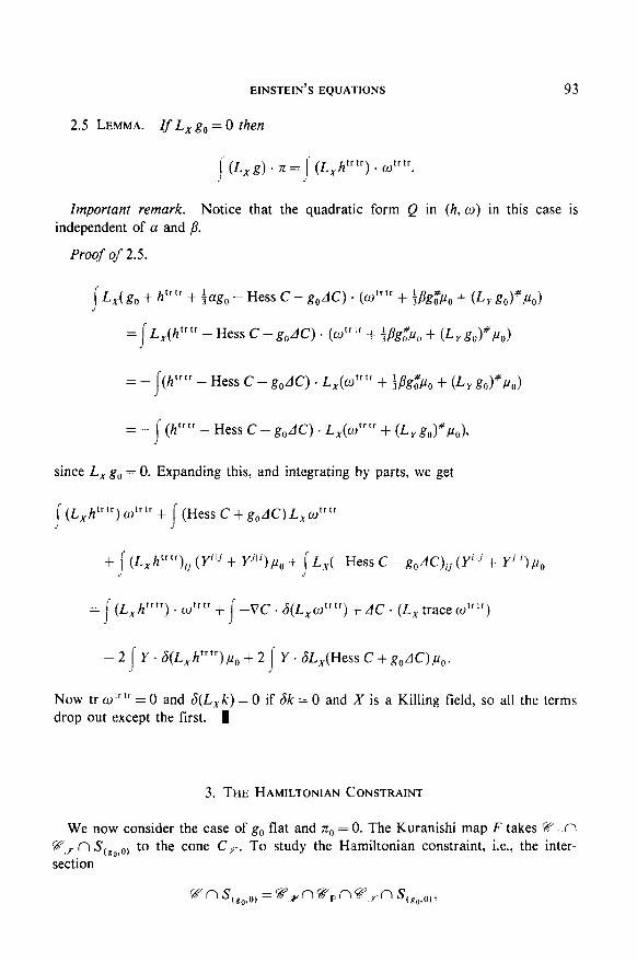
2.5 LEMMA. If L,g, = 0 then
93
(_ (L,g). 7c= I’(L,h”“). cdrtr.
Important remark. Notice that the quadratic form Q in (h, w) in this case is independent of a and /3.
Proof of 2.5.
! *L,(g,+ htrtr + iag,, - Hess C - g,dC) . (mtr” + $pg&, + (L,. g,)“p,,)
= I
L,(h”” - Hess C -g&C) . (w” tr + $3g&, + (L, g,)“cr,)
= - I
(,t*t* - Hess C - g,dC) . Lx(utrtr + $g&, + (L,g,)#,u,,)
Hess C - g,dC) . L,(cc)“~~ + (L, g,)#,Q
since L, g, = 0. Expanding this, and integrating by parts, we get
(LXht’t’) wt’t’ + (Hess C + g,dC) LXw””
+ ,f (Lxhtrtr)ij (Y’lj + Yj”)p,, + 1 L,y(-F[ess C - g,dC), (Yi’,j + Y”‘)p,,
= ,(LXhtrtr) . wtrtr !
+ -VC . G(Lxwtrtr) t AC . (L, trace utr tr)
- 2 j Y. 6(L,h”“),uUo + 2 j Y. GL,(Hess C + g,dC)pu,.
Now tr w” tr = 0 and d(L,k) = 0 if 6k = 0 and X is a Killing field, so all the terms drop out except the first. 1
3. THE HAMILTONIAN CONSTRAINT
We now consider the case of g, flat and z,, = 0. The Kuranishi map F takes F’,n
cn %,),W to the cone C,,. To study the Hamiltonian constraint, i.e., the inter- section
94 ARMS,MARSDEN,ANDMONCRIEF
it will be necessary to do some explicit calculations and make use of the fact that the cone C,, does not depend on the variables a and p (see 2.4 and 2.5). To carry this out, it will be more convenient to use the inverse Kuranishi map.
From 1.5 and 2.4 we have smooth mappings
Y(htrtr, a, 0” tr, /I) and C(hf’f’, a, utrtr, p>
which, together with their first derivatives, vanish at zero, and have the following property: for any a and /I and any (/ztrtr, w”‘~) satisfying
)‘(~xihtr’r)w’rtr=O, i= I,..., k, (3.1)
where X r ,..., X, are the Killing fields of g,, the data
g=g()+h”” + fag,, - Hess C - g,dC,
71 = otr tr + ~P&o + (LJ &J#Pu, (3.2)
lie in gP n g, n Scgo,oj. Thus, the mappings (Y, C) parametrize a full neighborhood of (g,, 0) in @,n @‘,n ScgO,,) in terms of solutions (/ztrtr, o”“) of (3.1) and (a,p). Note that cone (3.1) restricts (/ztrtr, mtrtr ) but leaves (a,/?) unrestricted.
Consider now the following afline submanifold of T*LX:
F = {(g, + h”, 0) E T*A 1 h” is covariant constant with respect to g,).
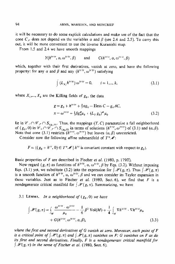
Basic properties of F are described in Fischer et al. (1980, p. 179ff). Now.regard (g, n) as functions of h” tr, a, wtr tr, p by Eqs. (3.2). Without imposing
Eqs. (3.1) yet, we substitute (3.2) into the expression for J~fg, z). Thus Jz( g, r) is a smooth function of h” tr, a, co” tr, /I and we can consider its Taylor expansion in these variables. Just as in Fischer et al. (1980, Sect. 6), we find that F is a nondegenerate critical manifold for sR( g, n). Summarizing, we have
3.1 LEMMA. In a neighborhood of (g,, 0) we have
+ G(hfrtr, utrtr, a,P), (3.3)
where the first and second derivatives of G vanish at zero. Moreover, each point of F is a critical point of s Z( g, 7~) and J Z( g, n) vanishes on F; G vanishes on F as do its first and second derivatives. Finally, F is a nondegenerate critical manifold for I Z( g, z) in the sense of Fischer et al. (1980, Sect. 6).
EINSTEIN’S EQUATIONS 95
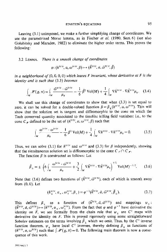
Leaving (3.1) unimposed, we make a further simplifying change of coordinates. We use the pa.rametrized Morse lemma, as in Fischer et al. (1980, Sect. 6) (see also Golubitsky and Marsden, 1982) to eliminate the higher order terms. This proves the following:
3.2 LEMMA. There is a smooth change of coordinates
cp: (htr tr, a, w” tr, p) ++ (h” tr, a, Gtr tr, j?)
in a neighborhood of (0, 0, 0,O) which leaves F invariant, whose derivative at F is the identity and is such that (3.3) becomes
-trtr
jMc;%yg,x)= j, Gtrt;ow LB’ Vol(M) + f j Vi”” . VP’p,. (3.4) hf
We shall use this change of coordinates to show that when (3.3) is set equal to zero, it can be solved for a double-valued function p = p*(htrtr, a, mtr tr). This will show that the solution set is tangent and diffeomorphic to the cone on which the Taub conserved quantity associated to the timelike killing field vanishes; i.e., to the cone CT defined to be the set of (htrtr, a, mtrtr, p) such that
w trtr
. 0”” -$8’vol(M)+$luVh”“. Vh”“p, = 0. (3.5)
PO
Thus, we can solve (3.1) for h”” and wtrtr and (3.3) for p independently, showing that the simultaneous solution set is diffeomorphic to the cone C p fI Cr.
The function /3 is constructed as follows: Let
& = * 6 j, ~‘r’r . cfjtrtr + ;i, vjptr . oprtrpo) “2 vo1pf-“2. (3.6)
PO
Note that (3.6) defines two functions of (htrtr, wtrtr), each of which is smooth away from (0.0). Let
tr tr (h, , a*, o;~~,/I*) = (p-‘(htrtr, G, fitrtr,&). (3.7)
This defines /I, as a function of (hfrtr, 5, titrtr) and mappings v* : (Jtrtr, c, Gtrtr) t-+ (htrtr, a+, WY”). From the fact that cp and o-’ have derivative the identity on F, we see formally from the chain rule that v* are C’ maps with derivative the identity on F. This is proved rigorously using some straightforward Sobolev estimates on the terms involving p, which we omit. Thus, by the C’ inverse function theorem, w* have local C’ inverses, thereby defining /I, as functions of
(h trtr, (r, mtrtr) such that jZ(g, z) = 0. The following main theorem is now a conse- quence of this work.
96 ARMS,MARSDEN,AND MONCRIEF
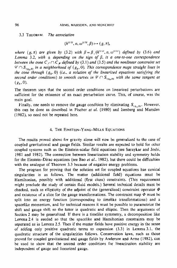
3.3 THEOREM. The association
(h lr tr, a, co” tr, p) I--+ (g, n),
where (g,z) are given by (3.2) with /j=/?*(htrtr,a,otrtr) defined b-v (3.6) and Lemma 3.2, with f depending on the sign of /I, is a one-to-one correspondence between the cone Cp n C., defined by (3.1) and (3.5) and the nonlinear constraint set
g n s~,o,o, in a neighborhood of (g,, 0). This correspondence maps straight lines in the cone through (g,, 0) (i.e., a solution of the linearized equations satisfying the second order conditions) to smooth curves in @n ScRoSOj with the same tangent at
(gw 0).
The theorem says that the second order conditions on linearized perturbations are sufftcient for the existence of an exact perturbation curve. This, of course, was the main goal.
Finally, one needs to remove the gauge condition by eliminating Sc,O,O,. However. this can be done as described in Fischer et al. (1980) and Isenberg and Marsden (1982), so need not be repeated here.
4. THE EINSTEIN-YANG-MILLS EQUATIONS
The results proved above for gravity alone will now be generalized to the case of coupled gravitational and gauge fields. Similar results are expected to hold for other coupled systems such as the Einstein-scalar field equations (see Saraykar and Joshi, 1981 and 1982). The connection between linearization stability and symmetry holds for the Einstein-Dirac equations (see Bao et al., 1982), but there could be difficulties with the analogue of Theorem 3.3 because of negative energy problems.
The program for proving that the solution set for coupled equations has conical singularities is as follows. The matter (additional field) equations must be Hamiltonian, possibly with additional (first class) constraints. (This requirement might preclude the study of certain fluid models.) Several technical details must be checked, such as ellipticity of the adjoint of the (generalized) constraint operator @ and existence of a slice for the gauge transformations. The constraint map @ must be split into an energy function (corresponding to timelike transformations) and a spacelike momentum, and for technical reasons it must be possible to parametrize the shift and gauge shift so the latter is quadratic and elliptic. Then the arguments of Section 2 may be generalized. If there is a timelike symmetry, a decomposition like Lemma 2.4 is needed so that the spacelike and Hamiltonian constraints may be separated as in Lemma 2.5. Then if the matter fields have positive energy in the sense of adding only positive quadratic terms to expansion (3.3) in Lemma 3.1, the quadratic structure of the singularities follows. Conservation laws, such as those proved for coupled gravitational and gauge fields by Anderson and Arms (1982), can be used to show that the second order conditions for linearization stability are independent of gauge and linearized gauge.
EINSTEIN’S EQUATIONS 97
The first few steps of this program have been carried out in previous papers for gravity calupled to gauge fields (Arms, 1979) and to certain massless scalar fields (Saraykar and Joshi, 1981 and 1982). Thus it is already known in these cases that the solution set can have singularities only at symmetric fields. In this section we complete the program for the gauge field case.’
As in the case of gravity alone, it suffices to study the constraint equations. We follow the notation of Arms (1979) except for some modifications noted below; calculations that appear in that reference are omitted.
Let 2l be the set of (WS*p, s > 3/p + 1) gauge field potentials on a Cauchy surface M in spacetime, i.e., connections on a fixed principal fiber bundle B over M. An element of VI will be represented by a Lie algebra-valued pseudotensorial one-form A on a neighborhood in M; A = u*w, where o is a local cross section of the bundle B and w is the connection. We assume that the Lie algebra admits an adjoint action invariant, positive definite inner product, denoted below by :. Let T*‘u be the (L’) cotangent bundle of 2I; thus q E Z’TU is a tensorial dual Lie algebra-valued vector density, the “negative electric field density,” and T*‘u is the phase space for the Yang-Mills field. Initial data for the coupled Einstein-Yang-Mills system are elements (g, A, 71, q) E P = T*(& x 2l), where -4, g, and 7c are as for gravity alone.
The constraint equations as given in Arms (1979) will not work in the program outlined above. The spacelike momentum comes in two pieces, the total super- momentum .X and a constraint .a’ on the Yang-Mills initial data which generalizes Gauss’ law. As stated in Arms (1979), (r, ,X) is not quadratic in (g, A. X, II), and this creates technical difficulties, as mentioned above. Fortunately, the situation is remedied Iby using, in essence, the old trick of adding a multiple of one constraint (in Dirac’s language, a “weakly zero” quantity) to another. In terms of the momentum mapping, this corresponds to choosing a different embedding of @, the diffeomorphism group on M, into the group S3 of bundle automorphisms (i.e., combined coordinate and gauge transformations) on B.
In the notation of Arms (1979) this procedure may be described as follows. The spacelike momentum (,P, .a) gives a contribution
H, = I
X. Y- + V:.X= {X’(-27~:,~ + &A& -Ay*j + C;,Af’A;)) M i M
+ V”(q’ + Cc A%$)} OlJ ab J C
to the total superhamiltonian. Here Cz, are the structure constant of the Lie algebra in a suitable basis. Integrating by parts one can re-express H, as
H,=l‘ X..?++ f.3, -M
I The case of the massless scalar field seems to be somewhat simpler than the present case. since there are no additional constraint equations. (The massive scalar field violates the strong energy condition, and several important steps in the program fail: see Saraykar and Joshi (1981) and especially (1982))
98
where
ARMS, MARSDEN, AND MONCRIEF
<5= -27c:,j + qjaA;,j - (qj,A&
= -27c:,j + q’,Aj4, - (rjj,Ay),j
and
The new supermomentum (7,X) is now quadratic and the constraints (3,X) = (0,O) are equivalent to (X,X) = (0,O). We shall give a more intrinsic description of this procedure below. To simplify the notation we write (4,X) for the new (quadratic) spacelike momentum and (X, I’) for the new generalized shift.
The pair 0 = (~P,~Z’) is the momentum map for the action of 3’ on P (via pullback). Now 3P3 is a semi-direct product of the diffeomorphism group Q3 and the gauge transformation group Y (bundle automorphisms that cover the identity). The group Y sits naturally in JS3, and has the momentum map X = 6 . v, where 6. indicates the doubly covariant divergence. On the other hand a3 has no natural copy in ~3’~. There is an action of 8’ on P, used in Arms (1979), which is most easily described in terms of its infinitesimal generators. An element of the Lie algebra of g3 is a vector field X on M. For each point (g, A, rc, q) E P, lift X horizontally to B, using the connection A. Let x indicate this lifted vector field, and let q be the tensorial object on B corresponding to r]. The infinitesimal generator at (g, A, 7c, ‘I) of the 33 action on P is then given by (L,g, a*Lp, L,n, a*Lxfj). (For a more concrete description, see Arms (1979), at the end of Section IIIB.) However, the momentum map for this action (S in the reference), is cubic in A and v.
To eliminate the cubic term, we proceed as follows. Choose a point (g,, A,,, no, qO) E P, and lift X horizontally with respect to A,. This lifted field generates an action on B which in turn gives rise via pullback to an action on P. The momentum map .P for this action is the new .P given above; in invariant notation, it is given by
where /I is the “magnetic field density” and x indicates the ordinary cross product in an orthonormal frame. (For more details on notation, see Arms (1979)).
The Hamiltonian Z for the coupled fields is given by
c-v= {n’ r 7c’ -f(trn’)*-R+$(~‘1~‘+/3’1P’)},u(g),
where rr’ is the tensor part of rc, and 1 indicates contraction using both metrics (g and the Lie algebra metric). Let @ = (Z, .P,X). This modification does not change the principal part of the operator D@, so the calculations in Arms (1979) show that D@* is elliptic. The coupled constraint equations are given by
@=O
EINSTEIN’S EQUATIONS 99
and the evolution equations are
(4.1)
where N and X are the lapse and shift of the spacelike slicing and V specifies the evolution of the Yang-Mills gauge. (Here J again represents the almost complex structure associated with the natural symplectic structure on the cotangent bundle P and the obvious L’metric.) From Eq. (4.1) one sees that a simultaneous symmetry of the fields is an element (N, X, v> E ker D@*, where N and X are the components of a Killing field (as for gravity alone) and V is the (infinitesimal) gauge transformation needed to preserve the gauge field potential under the Killing field flow.
Many of the arguments in the introduction and section one follow verbatim with the new Qi and obvious notational changes such as replacing (g, n), by (g, A, 7c, v) and (N, X) by (N, X, V). The fundamental decomposition, its interpretation, the orthogonal slice, the construction of the Kuranishi map F, and Propositions 1.1 through 1.5 all hold for the coupled case with no essential change in the proof.
The arguments of sections 2 and 3, dealing with spacelike and timelike constraints corresponding to particular symmetries, require a fairly explicit characterization of those symmetries on a constant mean curvature hypersurface M. By the arguments of Arms (1979, Sect. IVB) it follows that on M a symmetry (N, X, v> E ker D@* satisfies either (a) N = 0 (i.e., all symmetries are tangent to M), or (b) N is constant and the initial data is trivial (i.e., g and A are flat and 7~ and v are zero). In case (a), the “spacelike” case, there is a basis of ker D@* of the form {(0, Xi, Vi) 1 i = l,..., 1, Lxig = 0, Lxi7z = 0, Lxiq = [q, Vi] and L,,A = DV,}; in case (b), there is a basis with (l,O, 0) as one element and the rest of the basis like that in case (a).
Let ip, be the L* orthogonal projection onto the span of ((0, Xi, Vi)} and ip * the projection onto (1, 0,O). Thus the ith component of Ip, o @ is given by
i [xi..P+ vi:.lq
M
and
Itfollowsthatif~~={(g,A,71,rl)IiPo~=O},~~={(g,A,~,r7):IP,o~=O~,and ~~={(g,A,~r,rl)IIP,o~=O},then
t7=53$n5ge in case (a)
=FpnGYen%$ in case (b),
whereI--iP=IP,@lP,.
100 ARMS,MARSDEN,AND MONCRIEF
We first consider gp n go, analogous to G&n @F as in Section 2. For the Einstein-Yang-Mills case, we need something playing the role of a slice for the .J4 action. The mapping playing the role of the momentum map for this action is @ = (2, O), where 0 = (f,X). Thus, range JJ o D@* plays the role of the tangent space to the g4 orbit at (g,, A,, x,,, v,,)). As in Moncrief s decomposition ((M) in the introduction),
ker D@ o 9 = ker(DZ o S) n ker(DX o J) n ker(DR o JJ)
is the orthogonal complement to the orbit. Thus, as in Fischer et al. (1980, Sect. 5.5),
so = {(gorgon x0, rto)l + pv
where % is a suitably small ball in ker D@ o J (in a suitable Ws*p metric), plays the role of a slice for the 94 action.
Now we have, analogous to Theorem 2.1,
4.1 THEOREM. The map F maps SS$ n Ve n So locally l-l onto the cone
c, = I(go, ~0’~0’rl0)1 + {(h, b, w, 19) E ker D@ n ker D@ o J 1 Q(h, b, o, 0) = O),
where Q = P,(O - DO) = P,(@ -D@).
The proof is a straightforward generalization (by modification of notation) of the proof of Theorem 2.1.
In case (a), removing the gauges as in Fischer et al. (1980) completes the main results. For case (b), an analog to the decomposition in Lemma 2.4 is needed to separate the timelike (Hamiltonian) and spacelike constraints. Such a decomposition follows from Proposition 1.5 generalized to the coupled case and computations in Arms (1979): points (g, A, rr, v) E %p n So near (go, A,, no, qo) satisfying case (b) may be expressed as
g=g, + h”” +fag,-HessC-dCg,,
A =Ao+b”,
7c = (Jr” + (fPd + &4Y)POl
q = 8” - (DU)po,
(4.2)
where (C, Y, U) E domain of D@*, is a function of h” tr, bt’, w” tr, otr, a, and p given by the (generalized) Y map of Proposition 1.5, and bt’ and 8” have vanishing gauge covariant divergence.
Note that g and rz in Eq. (4.2) are unchanged from Section 2. Thus Lemma 2.5 remains valid in the coupled case, and Lemma 3.1 is unchanged except for the addition of a positive quadratic term
: Mwrl+Pv/~o. I
EINSTEIN’S EQUATIONS 101
Then the lrest of the proof of the conical structure of FP n go f-7 gX follows exactly as before.
Thus woe obtain the following when g, and A, are flat and rrO = 0, ‘lo = 0.
4.2 THEOREM. There is a l-1 correspondence between a neighborhood of (g,, A,, O., 0) in the cone C, f-? C, f~ S, and a neighborhood of ( g,, A,, 0,O) in the nonlinear constraint set %Y n S, which maps straight lines in the cone through (g,, A,, O., 0) to a smooth curve in F n S, with the same tangent at (g,, A,, 0,O).
This result has the same interpretation as for gravity: solutions of the linearized constraint equations are nonspurious, i.e., are linearization stable, if and only if the second order conditions 0 = j+,,., (N,X v>. D*@(g,,& ~0, rl,)((h, b, 0, S), (h, b, w, 0)) are satisfied on the hypersurface. As we have already mentioned, these second order conditions are actually hypersurface and gauge invariant, using the conservation laws of Anderson and Arms (1982).
5. DISCUSSION
This paper completes our study of linearization stability and the local structure of the space of solutions for the Einstein and Einstein Yang-Mills equations on spacetimes possessing a compact Cauchy surface with constant mean curvature. We have shown that the space of solutions has a quadratic singularity at every solution possessing a group of symmetries of dimension at least one. Using second order conditions, we have identified those linearized solutions which can be used in an honest perturbation expansion. This section discusses a few miscellaneous issues relevant to our results.
The Second Order Conditions
For vacuum gravity, the necessary and sufficient conditions that a linearized solution (4’h at (4)go be tangent to a curve “‘g(L) of exact vacuum solutions satisfying “)go = (4)g(0) is that the Taub conserved quantities vanish identically,
I ‘4’X . [D2 Ein(‘4’go) . ((4)h, “‘h)] . (4)Zz d3C = 0
-r
for all killing fields (4)X of the metric (4)go. These quantities comprise the momentum map for the isometry group of (4)go acting on the linearized theory. (For purely spacelike symmetries one can show this directly. For a timelike symmetry this is the known fact that i s, (1,0) . D*@( g, O)((h, w), (h, w)) d3Z is a Hamiltonian for the perturbations-this is the second variation method.)
The proofs in Fischer et al. (1980) and the present paper on the space of solutions worked with the constraint equations directly. The role of the Taub quantities is to show that the order conditions are hypersurface independent and gauge invariant.
In Section 4 we treated the Einstein-Yang-Mills equations by studying the
102 ARMS, MARSDEN, AND MONCRIEF
constraints on a given hypersurface. To show analogously that the conditions are hypersurface independent and gauge invariant, and hence an intrinsic property of the spacetime solution set, one needs the Einstein-Yang-Mills analogue of the conserved Taub quantities treated from a covariant point of view. This aspect may be found in Anderson and Arms (1982).
The Symplectic Space of True Degrees of Freedom
If one wishes to divide out by the gauge group (diffeomorphisms of spacetime for gravity, bundle automorphisms over the identity for Yang-Mills and bundle automorphisms over diffeomorphisms for the Einstein-Yang-Mills equations), then a suitable slice theorem is needed. For the pure Yang-Mills equations (with a compact group), such a slice theorem is relatively routine (see, for example, Singer, 1978, Babelon and Vialett, 1981, and Kondracki and Rogulski, 1981). For vacuum gravity, see Isenberg and Marsden (1982). Using a combination of the methods from these papers should enable one to prove a slice theorem for the Einstein-Yang-Mills equations.
Using such a slice theorem, the results of Fischer et al. (1980), this paper and Arms et al. (1981) (especially Lemma IS), one can show that the space of solutions modulo gauge transformations is a stratified symplectic manifold, i.e., a stratified manifold, each stratum of which is symplectic. The procedure for vacuum gravity is spelled out in Isenberg and Marsden (1982). It is also shown there, using the slice theorem and York parametrization, that the generic points consisting of spacetimes with no symmetries is an open dense set. Thus the generic symplectic stratum in the reduced space is also open and dense.
For pure Yang-Mills fields, the results of Arms (1981) can similarly be used to establish the analogous results in that case. For the Einstein-Yang-Mills equations the symplectic stratification follows from the results of Section 4, this paper, and an Einstein-Yang-Mills slice theorem.
Respecting Symmetry Types
In the context of general momentum mappings, Arms et al. (1981) Theorem 4’ showed that the Kuranishi map preserves the symmetry type for any Lie subalgebra 8 = S,()? the symmetry (= isotropy) algebra of x,,. That is, solutions of the nonlinear problem with symmetry type 8 are mapped to those elements in the cone consisting of the linearized solutions satisfying the second order conditions and having the same symmetry type 8.
For the momentum constraints and for the Yang-Mills constraints, this remains true by essentially the same methods. This is also basically true for the full constraints as well, but the Hamiltonian constraint must be treated by a separate argument. If (4)g0 has a timelike Killing field, then (4)g0 is flat and we may choose Z so that tr k = 0. If we are looking for nearby solutions which also have a timelike Killing field, then this amounts to studying the space of flat 3-metrics which can be done as in Fischer and Marsden (1975). If 8 does not include time translations then the result can be dealt with by the Kuranishi method.
EINSTEIN’S EQUATIONS 103
We note that with C fixed, rc = 0 and g flat, g can change its spacelike isometry group; i.e., there can be branching within the flat metrics. However, this cannot happen for Z = T3; this follows from Proposition 8.1 of Fischer et al. (1980).
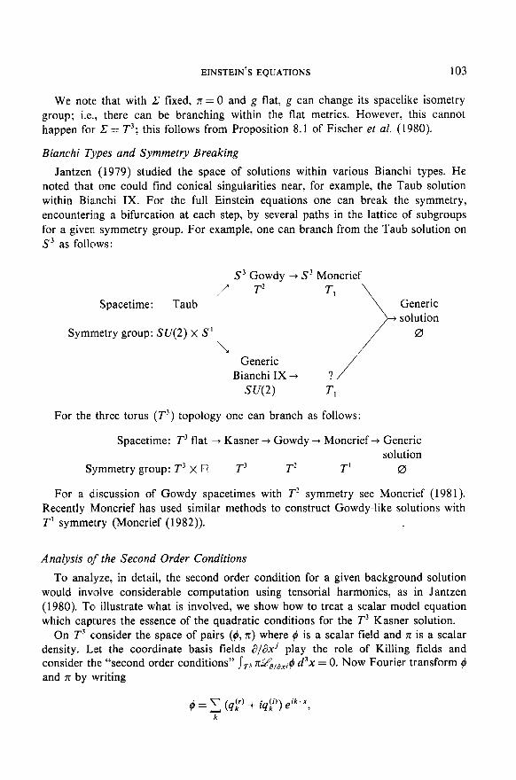
Bianchi Types and Symmetry Breaking
Jantzen (1979) studied the space of solutions within various Bianchi types. He noted that one could find conical singularities near, for example, the Taub solution within Bia.nchi IX. For the full Einstein equations one can break the symmetry, encountermg a bifurcation at each step, by several paths in the lattice of subgroups for a given. symmetry group. For example, one can branch from the Taub solution on S3 as follows:
S3 Gowdy + S3 Moncrief /” TZ T,
Spacetime: Taub
Symmetry group: SU(2) X S’ \
Generic Bianchi IX + ? .;
Generic solution
0
SW) T,
For the three torus (T3) topology one can branch as follows:
Spacetime: T3 flat + Kasner + Gowdy + Moncrief + Generic solution
Symmetry group: T3 x R T3 T2 T’ 0
For a d.iscussion of Gowdy spacetimes with T2 symmetry see Moncrief (198 1). Recently Moncrief has used similar methods to construct Gowdy-like solutions with T’ symmetry (Moncrief (1982)).
Analysis qf the Second Order Conditions
To anal:yze, in detail, the second order condition for a given background solution would involve considerable computation using tensorial harmonics, as in Jantzen (1980). To illustrate what is involved, we show how to treat a scalar model equation which captures the essence of the quadratic conditions for the T3 Kasner solution.
On T3 c:onsider the space of pairs (4, Z) where 4 is a scalar field and rc is a scalar density. Lset the coordinate basis fields a/ax’ play the role of Killing fields and consider the “second order conditions” I,, Zga,axj $ d3x = 0. Now Fourier transform 4 and 7c by writing
Q = 5 (4:’ + is:)) eik’x, k
104
and
ARMS, MARSDEN, AND MONCRIEF
where k ranges over the appropriate discrete lattice for T3. The linear reality conditions q f) = 4”: ant) p$ = -pyL, etc., that restrict the q’s and p’s are assumed satisfied.
The second order conditions take the form
Changing variables according to qf’ = (l/@)(Q;’ + I’;‘), py’ = (l/d) (Pr’ - Qy’), etc., and restricting the sum to range only over the independent k’s (note that k and -k give the same contribution), we get
Now choose three independent lattice vectors such as e”’ = (1, 0, 0), e’*’ = (0, 1,0) and ec3) = ( 0, 0, 1) and rewrite the second order conditions as
(Pg,)* - (Qg,)’ = Rj(Q, f’), j= 1, 2, 3.
The crucial point is that R, does not depend upon {Pi:{,, Qs!,, P(” Qz%, PL$,, et*,, Q$,}, and similarly for R, and R,. This can be seen by inspection from the above expressions. Thus we can choose the variables in the set complementary to (QFJ,, Pg,} arbitrarily and then solve the three independent “cone” equations
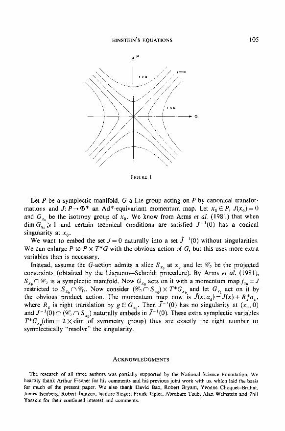
(PF$)* - (Q$)’ = Rj(Q, P) = rj.
Thus the singularity structure is that of P2 - Q’ = r with r a variable parameter. See Fig. 1.
The divergence constraint in relativity for the T3 Kasner solution is similar; indeed the tensor indices decouple and do not materially affect the above arguments.
Resolving Singularities2
The question of resolving the singularities in the space of solutions may be important for quantization or other purposes (cf. Sniatycki, 1982). What we seek is to include our solution space into the solution space for a modified problem with no singularities. We describe the idea in a general symplectic context, as in Arms et al. (1981).
* We thank R. Bryant for remarks on “marked surfaces” which motivated the discussion here.
EINSTEIN’S EQUATIONS 105
FIGURE I
Let P be a symplectic manifold, G a Lie group acting on P by canonical transfor- mations and J: P-1 t5* an Ad*-equivariant momentum map. Let x,, E P, J(x,) = 0 and G,. be the isotropy group of x,,. We know from Arms et al. (1981) that when dim G,, > 1 and certain technical conditions are satisfied J-‘(O) has a conical singularity at x0.
We want to embed the set J= 0 naturally into a set J-‘(O) without singularities. We can enlarge P to P x T*G with the obvious action of G, but this uses more extra variables than is necessary.
Instead, assume the G-action admits a slice S,, at x0 and let @& be the projected constraints, (obtained by the Liapunov-Schmidt procedure). By Arms et al. (198 l), SXO n gP is a symplectic manifold. Now G,, acts on it with a momentum map j,” = J restricted to S,0 n 5?$. Now consider (‘?$ n SX,) x T*Gxo and let G,” act on it by the obvious product action. The momentum map now is J(x, a,) = J(x) + R,*a,, where R, is right translation by g E G,.. Then I-‘(O) has no singularity at (x,, 0) and J-‘(O) f7 (FP fl S,J naturally embeds in J-‘(O). These extra symplectic variables T*G,&dim = 2 x dim of symmetry group) thus are exactly the right number to symplectically “resolve” the singularity.
ACKNOWLEDGMENTS
The research of all three authors was partially supported by the National Science Foundation. We heartily thank Arthur Fischer for his comments and his previous joint work with us. which laid the basis
for much of the present paper. We also thank David Bao, Robert Bryant, Yvonne Choquet-Bruhat, James Isenbtag, Robert Jantzen, Isadore Singer, Frank Tipler, Abraham Taub, Alan Weinstein and Phil Yasskin for their continued interest and comments.
106 ARMS, MARSDEN, AND MONCRIEF
REFERENCES
I. ANDERSON AND J. ARMS (1982). In preparation.
J. ARMS (1979). J. Math. Phys. 20 443-453. J. ARMS (1981). Math. Proc. Cambridge Philos. Sot. 90 361-372. J. ARMS, J. MARSDEN, AND V. MONCRIEF (1981). Commun. Mafh. Phys. 78 455-478.
M. F. ATIYAH, N. J. HITCHIN. AND I. M. SINGER (1978). Proc. R. Sot. London Ser. A 362 425-461. 0. BABELON AND C. M. VIALLET (1981). Commun. Math. Ph.vs. 81 515-525.
D. BAO, J. ISENBERG. AND P. YASSKIN (1982). In preparation.
D. BRILL AND S. DESER (1973). Commun. Math. Phys. 32 291-304. A. FISCHER AND J. MARSDEN (1975). Duke Math. J. 42 519-547.
A. FISCHER, J. MARSDEN. AND V. MONCRIEF (1980). Ann. Inst. Henri Poincare 33 147-194. M. GOLUBITSKY AND J. MARSDEN (1982). The Morse lemma in infinite dimensions via singularity
theory, SIAM J. Math. An., in press. J. ISENBERG AND J. MARSDEN (1982). Ph.vs. Rep., in press.
R. JANTZEN (1979). Commun. Math. Phvs. 64 21 l-232. R. JANTZEN (1980). In “Essays on General Relativity” (F. Tipler, Ed.), Academic Press, New York. W. KONDRACKI AND J. ROGULSKI (1981). The stratification structure in the space of gauge equivalent
Yang-Mills connections, preprint. M. KURANISHI (1965). In “Proceedings of Conference on Complex Analysis, Minneapolis. 1964” (A.
Aeppli et al., Eds), Springer-Verlag, Berlin/New York. J. MARSDEN AND F. TIPLER (1980). Phys. Rep. 66 109-139.
J. MARSDEN AND A. WEINSTEIN (1974). Rep. Math. Phys. 5 121-130. V. MONCRIEF (1975). J. Math. Phys. 16 493-498.
V. MONCRIEF (1976). J. Math. Phys. 17 1893-1902. V. MONCRIEF (1977). Ann. Phys. 108 387400.
V. MONCRIEF (1981). Ann. Phys. 132 87-107. V. MONCRIEF (1982). Ann. Phys. 141, 83-103.
J. MORROW AND K. KODAIRA (1971). “Complex Manifolds,” Holt, Rinehart and Winston, New York.
R. V. SARAYKAR AND N. E. JOSHI (1981). J. Math. Phys. 22 343-347. R. V. SARAYKAR AND N. E. JOSHI (1982). J. Math. Phys. 23, 1738.
I. M. SINGER (1978). Commun. Math. Phys. 60 7-12. J. SNIATYCKI (1982). In “Proceedings, Summer School on Theoretical Physics, Clausthal,” to appear.
A. J. TROMBA (1976). Can J. Math. 28 64&652.