Embed Size (px)
Citation preview
Forschungsinstitut zur Zukunft der ArbeitInstitute for the Study of Labor
DI
SC
US
SI
ON
P
AP
ER
S
ER
IE
S
The Subversive Nature of Inequality:Subjective Inequality Perceptions and Attitudesto Social Inequality
IZA DP No. 9406
October 2015
Andreas Kuhn
The Subversive Nature of Inequality:
Subjective Inequality Perceptions and Attitudes to Social Inequality
Andreas Kuhn Swiss Federal Institute for Vocational Education and Training,
University of Lucerne and IZA
Discussion Paper No. 9406 October 2015
IZA
P.O. Box 7240 53072 Bonn
Germany
Phone: +49-228-3894-0 Fax: +49-228-3894-180
E-mail: [email protected]
Any opinions expressed here are those of the author(s) and not those of IZA. Research published in this series may include views on policy, but the institute itself takes no institutional policy positions. The IZA research network is committed to the IZA Guiding Principles of Research Integrity. The Institute for the Study of Labor (IZA) in Bonn is a local and virtual international research center and a place of communication between science, politics and business. IZA is an independent nonprofit organization supported by Deutsche Post Foundation. The center is associated with the University of Bonn and offers a stimulating research environment through its international network, workshops and conferences, data service, project support, research visits and doctoral program. IZA engages in (i) original and internationally competitive research in all fields of labor economics, (ii) development of policy concepts, and (iii) dissemination of research results and concepts to the interested public. IZA Discussion Papers often represent preliminary work and are circulated to encourage discussion. Citation of such a paper should account for its provisional character. A revised version may be available directly from the author.
IZA Discussion Paper No. 9406 October 2015
ABSTRACT
The Subversive Nature of Inequality: Subjective Inequality Perceptions and Attitudes to Social Inequality*
This paper shows that higher levels of perceived wage inequality are associated with a weaker (stronger) belief into meritocratic (non-meritocratic) principles as being important in determining individual wages. This finding is robust to the use of an instrumental-variable estimation strategy which takes the potential issue of reverse causality into account, and it is further corroborated using various complementary measures of individuals’ perception of the chances and risks associated with an unequal distribution of economic resources, such as their perception of the chances of upward mobility. I finally show that those individuals perceiving a high level of wage inequality also tend to be more supportive of redistributive policies and progressive taxation, and that they tend to favor the political left, suggesting a feedback effect of inequality perceptions into the political-economic sphere. Taken together, these findings suggest that high levels of perceived wage inequality have the potential to undermine the legitimacy of market outcomes. JEL Classification: D31, D63, J31 Keywords: inequality perceptions, attitudes to social inequality, support of redistribution, legitimacy of market outcomes, beliefs about the causes of economic success, political preferences Corresponding author: Andreas Kuhn Swiss Federal Institute for Vocational Education and Training Kirchlindachstrasse 79 3052 Zollikofen Switzerland E-mail: [email protected]
* I thank Hans Pitlik, Justina Fischer, Alois Stutzer, and several participants at the 2013 Annual Meeting of the European Public Choice Society for helpful comments and suggestions on an early draft of this paper, and Sally Gschwend-Fisher for proofreading the manuscript.
1 Introduction
Many OECD countries have seen significant increases in inequality in the past few decades,
including the United States as well as several continental European countries (e.g. Atkinson,
2008). Besides their direct and obvious impact through the re-allocation of economic resources
to and from different socio-economic groups, changes in a country’s aggregate distribution might
also have repercussions in the political-economic sphere if they influence individuals’ beliefs
about the legitimacy of market outcomes. Indeed, several theoretical papers (e.g. Alesina and
Angeletos, 2005; Alesina et al., 2012; Benabou and Tirole, 2006) made a convincing argument
that changes in the aggregate level of inequality might influence individuals’ attitudes towards
social inequality, such as their beliefs about the importance of non-meritocratic principles in
determining individual wages, and that these changes in attitudes might eventually feed back
into the effective distribution of economic resources because they might affect distributional
parameters ultimately set by voters, such as marginal tax rates on income.
The goal of this paper is to directly test the hypothesis that inequality affects the legitimacy
of market-based outcomes. The paper presents, against this broader background, empirical es-
timates of the effect of individuals’ subjective perceptions of wage inequality in their country of
residence on their attitudes to social inequality, focusing on individuals’ subjective beliefs that
meritocratic, or non-meritocratic, factors are important in determining wages. In contrast to
most previous studies on the topic, however, this paper focuses on a broad array of attitudes
the perceived level of inequality potentially affects, rather than only on a single attitudinal
measure.1 The second key feature of this study is that the empirical analysis is based on an
individual-level measure of subjective inequality perceptions, rather than on some objective
and highly aggregated measure of inequality. Using a unique measure of individual-level per-
ceptions of wage inequality, I find that higher levels of perceived inequality are significantly and
substantively associated with a stronger (weaker) belief in labor markets functioning according
to non-meritocratic (meritocratic) principles. In this sense, a higher perceived level of wage
inequality indeed appears to subvert the legitimacy of market outcomes. This result holds true
1While previous evidence has mostly focused on the impact of inequality on subjective wellbeing, bothBjørnskov et al. (2013) and Schneider (2012) have argued that the perceived fairness of the wage distributionmediates the effect of inequality on wellbeing, suggesting that a focus on a broader set of outcomes might yieldinteresting insights into the overall attitudinal effects of inequality. Note, however, that neither of these studieshas estimated the direct effect of inequality (perceptions) on attitudes.
1
when I account for potential reverse causality using an instrumental-variable approach, and
I further corroborate it using a variety of complementary outcomes reflecting an individual’s
perceptions of the chances and risks associated with an unequal distribution of wages, his or
her attitudes towards the role of government and progressive taxation, as well as his or her
general political preferences. In line with the results for individuals’ beliefs about the reasons
for getting ahead, these additional estimates show that higher inequality perceptions lead to
a stronger (weaker) awareness or salience of the risks (chances) potentially associated with
inequality, as well as a stronger support of government intervention aiming to reduce existing
inequalities, of progressive taxation, and of the political left. Finally, and importantly, I also
find that those individuals with higher inequality perceptions are less satisfied with their own
wages.2
The key conceptual challenge in addressing these questions empirically is the need for an
individual-level measure of inequality perceptions. Simply relying on a more or less easily
available objective, yet also highly aggregated, measure of inequality would ignore the fact
that people appear to hold widely different, and often heavily biased perceptions of the overall
distribution of economic resources (e.g. Chambers et al., 2014; Cruces et al., 2013; Kuhn, 2011;
Norton and Ariely, 2011; Osberg and Smeeding, 2006).3 If we acknowledge that individuals
have different, and presumably biased, perceptions of wage inequality, the use of an objective
measure of inequality in the empirical analysis would simply fail to reflect heterogeneity of this
kind, potentially implying inconsistencies in the estimated effect of inequality on attitudes.4 In
fact, the available empirical evidence shows that individuals’ perceptions of wage levels and/or
inequality are, in part, directly related to socio-economic factors (e.g. Kuhn, 2011; Schneider,
2012), suggesting that part of the observed variation in individual-level (mis-)perceptions of
inequality is indeed of a systematic nature (implying a potential bias when this source of
variation is ignored when estimating the impact of inequality on attitudes). To take these
2This last finding is insofar especially important as it allows me to directly relate my findings to the existingempirical evidence on the subject which has, as discussed in more detail below, up until now almost exclusivelyfocused on the association between inequality and individuals’ subjective wellbeing (Senik, 2005, provides asurvey of this literature).
3Other studies have focused on individual perceptions of alternative economic phenomena, such as tax rates(Gemmell et al., 2004) or corruption (Olken, 2009).
4There is, of course, also a more practical reason for favoring individual-level inequality perceptions overaggregate-level inequality measures. Because there is much more variation in individual-level inequality percep-tions, it will presumably be easier to get reasonably precise estimates when using inequality perceptions ratherthan some objective measure of inequality.
2
issues into account, the empirical analysis of this paper will therefore be based on a simple yet
intuitive empirical measure of individual-level inequality perceptions, following the procedure
proposed by and described in more detail in Kuhn (2011).
In contrast to the approach chosen in this paper, however, most previous papers studying
the impact of inequality on individuals’ attitudes used some objective, rather than subjective,
measure of inequality as their key regressor – assuming, at least implicitly, that people correctly
perceive the prevailing level of inequality. While earlier studies focused on highly aggregated
measures of inequality (Verme, 2011, provides a survey of studies focusing on the association be-
tween country-level inequality measures and individual-level measures of subjective wellbeing),
more recent studies have shifted their focus towards more disaggregated measures of inequality,
arguing that people do not care as much about the aggregate distribution of market wages
as they care about the comparison to smaller and much more specific reference groups, such
as their coworkers, their friends, and/or their neighbors.5 The latter group of studies does
allow for variation in inequality perceptions across individuals, but only because of different
comparison groups, not because of biased perceptions of wages or wage differentials per se.
Remarkably, these studies consistently tend to find a negative association between inequal-
ity and subjective wellbeing, independent of the exact definition of the comparison group.6 For
example, Clark and Oswald (1996) show in a sample of British workers that both job and wage
satisfaction are significantly and negatively associated with an individual’s comparison income,
given by the predicted wage from a conventional wage regression, while holding the absolute
level of income constant. Ferrer-i-Carbonell (2005) reports a similar result for Germany. She
defines individuals with similar education, age, and location of residence as the comparison
group and finds that well-being increases the larger an individual’s income is with respect to
that of the comparison group while holding the absolute level of income constant. Luttmer
(2005), in contrast, matches individual-level survey data to information on local average house-
hold incomes from representative survey data from the US, using a strictly spatially defined
comparison group. He finds that, even after controlling for an individual’s own income, self-
5This lines up well with Clark and Senik (2010), who find that most individuals, if asked directly, confirmthat such comparisons are at least somewhat important for them. Moreover, individuals most often comparethemselves with their colleagues (i.e. their coworkers).
6Only few papers have directly focused on behavioral, instead of attitudinal, effects of inequality, such as onindividual work effort. In contrast to the (much larger) literature focusing on subjective wellbeing, the findingsare considerably more mixed (e.g. Charness and Kuhn, 2007; Clark et al., 2010; Cornelissen et al., 2011).
3
reported happiness is lower the higher average earnings are in an individual’s neighborhood.
Clark et al. (2009), using a similar approach and using data from Denmark, show that subjective
well-being depends on one’s relative rank within narrowly defined neighborhoods. Similarly,
Schwarze and Harpfer (2007) report a negative relation between pre tax-and-transfer inequal-
ity and life satisfaction across regions in West Germany, while Winkelmann and Winkelmann
(2010) report a negative association between aggregate-level inequality measures and economic
wellbeing across municipalities in Switzerland as well.
The assumption that people have unbiased perceptions of the prevailing level of inequality
has, however, been relaxed in two more recent studies. Both studies manipulate individuals’
information about wage differentials in a field experiment. Both studies provide indirect evi-
dence of people potentially having misperceptions of the true level of inequality, since a minor
information treatment is able to influence individuals’ attitudes. In the first of these studies,
Card et al. (2012) randomize the access to information about coworkers’ wages in a sample
of university employees, providing arguably more compelling evidence on the causal effect of
coworkers’ wages on one’s job satisfaction than most studies mentioned so far. Consistent with
the evidence from the majority of observational studies, however, they also find that com-
parison income has a strong negative effect on individual job satisfaction. Finally, in another
randomized field experiment, Kuziemko et al. (2015) manipulate individuals’ information about
income inequality. They find that providing individuals with this information has large effects
on whether inequality is viewed as a pressing problem, but only small effects on individuals’
support for governmental intervention with regard to the distribution of income.
Finally, yet on a somewhat more general level, this paper also adds to the small number
of empirical studies documenting that economic events or circumstances influence individuals’
attitudes and beliefs. In one of these studies, for example, Di Tella et al. (2007) show that
granting property rights to squatters strongly influences their market beliefs. Similarly, Giuliano
and Spilimbergo (2014) show that the macroeconomic context at the time of youth (i.e. growing
up during a boom versus during a recession) influences individuals’ beliefs about the importance
of own effort and luck in getting ahead, their demand for redistribution, as well as their trust in
public institutions. In line with the results from these studies, this paper shows that attitudes
towards inequality are, in part, shaped by the prevailing level of inequality, and thus the paper
4
also adds to our general understanding of how attitudes and preferences are formed and how
they evolve over time.
The remainder of this paper proceeds as follows. The next section presents the data sources
and discusses the selection of the sample as well as the construction of the key variables, i.e.
attitudes to social inequality and individual-level inequality perceptions. Section 3 presents a
few descriptives for the key variables. Section 4 discusses the econometric framework, while
section 5 presents and discusses the resulting estimates. Section 6 concludes.
2 Data and Measures
2.1 Data Source
The empirical analysis fully relies on data from the “Social Inequality” cumulation of the years
1987, 1992, 1999, and 2009 (ISSP Research Group, 2014a,b). These data are a collection of
several national-level surveys focusing specifically on attitudes to social inequality, administered
and made available by the International Social Survey Programme (ISSP).7 They represent one
of the best available sources of quantitative data to study individuals’ perceptions of inequality
and their attitudes to social inequality across countries and over time.
One of the key advantages of these data is that they cover a large number of observations
from various countries and that they stretch over a relatively long period of time, for at least
a subset of the participating countries (appendix table A.1 shows the number of individual
observations by country and year). Another attractive feature of the data is that they contain
a large number of items related to individuals’ attitudes to social inequality, including, for
example, individuals’ beliefs about the causes of economic success or their stated support of
progressive taxation. On the other hand, however, there have been many changes to the survey
design over time, with the practical consequence that the number of items available in all four
rounds of the survey is rather limited (more on this below; see sections 3.1 and 4.2).
7More information is available from the organization’s website (www.issp.org). The data are available toresearchers from the GESIS data archive (www.gesis.org/en/issp/home).
5
2.2 Sample Selection
The sample used in the main part of the empirical analyses is determined by the availability of
the dependent variable and the key regressor (i.e. individual-level inequality perceptions). As
noted above, relatively few of the survey items are available in identical form in all four years of
the survey. This implies that there are potentially large differences in the effective sample size for
the different outcome measures, irrespective of any additional nonresponse issues. Fortunately,
however, the series of items used to construct the key regressor are available in all four years
(though not necessarily for all countries) in principle, but there have been a few changes over
time to that set of items as well (cf. footnote 9 below).
2.3 Attitudes to Social Inequality
The following paragraphs discuss the various outcome measures available from the ISSP surveys
(see also table 1, which contains the full list of survey items used as outcomes, and which is
discussed in more detail in section 3.1 below).
Beliefs About the Causes of Economic Success
The outcome measures of primary interest are several attitudinal questions from the ISSP
surveys which explicitly focus on individuals’ beliefs about the causes of economic success.
Overall, there are twenty-six different items dealing with individuals’ beliefs on this issue, and
they can be further grouped into three distinct sets of items describing different dimensions of
individuals’ beliefs about the causes of economic success, namely: (i) beliefs about the reasons
for getting ahead, (ii) beliefs about the incentivizing effect of inequality, and (iii) pay norms.
Note that the first two sets of items relate to individuals’ perception of the wage-setting process,
while the third set of items asks individuals about their normative views regarding the factors
that should ideally be important in determining wages.
The first group of items asked individuals about the reasons, from their subjective point of
view, for getting ahead in their country of residence. For example, one of the items in this group
asked respondents whether they thought that coming from a wealthy family was important for
getting ahead (here, as for most other items, respondents could indicate their agreement with
the statement on a five-point scale running from one to five; see table 1 for details). Because
6
this group of items contains variables describing both meritocratic (e.g. education and effort)
as well as non-meritocratic (e.g. knowing the right people) mechanisms, an even more nuanced
analysis of this specific dimension of attitudes to social inequality will be possible.
Then there are, secondly, several questions asking individuals’ whether they believe that
inequality has, at either the individual or the aggregate level, an incentivizing effect on economic
actors. For example, respondents were asked whether they thought that wage differentials
between people with different educational attainment are necessary as an individual incentive
for choosing a higher educational attainment in the first place, or whether they thought that
large differences in pay are necessary for a country’s prosperity.
Finally, a third set of items asked individuals to state how wages should ideally be deter-
mined from their point of view. In other words, individuals were asked about their subjective
pay norms (somewhat mirroring the first group of items, which asked them about the actual
mechanisms determining pay). Here, for example, people were asked to state whether they
thought that individual pay should be determined according to the attained level of education,
or whether they would prefer compensation to depend on whether someone has to support
children. As for individuals’ beliefs about the reasons for getting ahead, it is also possible to
distinguish between pay norms related to either meritocratic or non-meritocratic principles.
The Perception of Chances and Risks Associated with Inequality
A second broader subject the survey covers, composed of a total of eleven distinct items,
describes individuals’ perceptions of both chances and risks potentially associated, at least in
respondents’ perceptions, with economic resources being distributed more or less unequally.
The main hypothesis here is individuals who perceive wage inequality to be higher will tend to
perceive chances to be less obvious and risks to be more relevant than individuals who perceive
inequality to be low.
A first item of interest in this context asked individuals whether they thought that they
“stand a good chance of improving their standard of living”, which might be thought of as a
subjective measure of perceived upward mobility. One might hypothesize that those individuals
who perceive a high level of inequality are, ceteris paribus, less likely to agree with this statement
if they, as argued above, perceive that non-meritocratic factors drive wage differentials. That is,
7
assuming that people perceive access to higher wages to be mainly driven by non-meritocratic
mechanisms, it appears likely that those who perceive a high level of wage inequality are less
likely to believe in their own upward-mobility.
Another potentially interesting outcome in this context is individuals’ satisfaction with their
own wages. Again, if individuals believe that wages are (co-)determined by factors beyond an
individual’s control, such as coming from a wealthy family or having well-educated parents,
then we would probably also expect them to be less satisfied with their own wages (i.e. an
individual’s own compensation from work likely appears unfair, relative to those with higher
wages, if higher wages are mostly achieved through factors not related to one’s own ability or
effort).8
A third item of interest describes individuals’ normative assessment of the overall level of
inequality (as they personally perceive it). In this regard, respondents were directly asked to
state if they thought that “income differences are too large” in their country of residence. Note
that the item does not ask about the perception of the absolute level of inequality, but about
the perceived level of inequality relative to some legitimate level.
Fourth and finally, individuals were also asked to evaluate whether any broader conflicts
exist in society from their point of view, such as between the poor and the rich, or between
unemployed and employed workers. The hypothesis here is that a higher perceived level of wage
inequality goes hand in hand with people being more likely to perceive more general conflicts
between different socio-economic groups in their society.
The Role of Government and Support of Progressive Taxation
A further set of interesting items relates to the proper role of government towards redistribution
and the provision of goods and services and to individuals’ explicit support of progressive
taxation. Again, if higher inequality perceptions are associated with a weaker belief in market
justice, one would presumably also expect that higher inequality perceptions go hand in hand
with a stronger support for government intervention and progressive taxation – to counteract
the perceived malfunctioning of markets in the allocation of economic resources.
In the survey, individuals were asked with regard to the role of government to evaluate
8Also, as noted in the introduction, almost all of the previous empirical papers on the subject have focusedexclusively on the association between inequality and some measure of wage or general satisfaction; this outcomethus also allows me to compare and relate my own results to that specific strand of the literature.
8
whether they thought that the government is responsible for offering access to several goods and
services such as providing a decent living standard for the unemployed. Regarding progressive
taxation, individuals had to evaluate whether people with high incomes should pay higher taxes,
or whether they thought that taxes for people with high income are high enough or not.
Political Preferences and Political Participation
Finally, the ISSP surveys also contain a few items on respondents’ general political preferences;
that is, their preferences towards either the political left or the political right, as well as their
participation at the most recent national-level elections. I aggregate the three available items
on political identification, as all three items ask about individuals’ party preferences, and I use
the remaining item on whether someone had voted at the last election in one’s country as a
rough measure of an individual’s political participation.
2.4 Inequality Perceptions and Distributional Norms
Inequality Perceptions
One of the most distinguishing features of the ISSP data on social inequality is a series of
questions about the level of compensation for people working in various specific occupations,
such as an unskilled worker in a factory or a doctor in general practice. For each of these
occupations, respondents in the survey were asked to estimate both the actual level of earnings
as well as the level of earnings that they would consider as legitimate (actual and ethical wage
estimates, for short, in the following).9
Noting that an individual’s set of actual wage estimates roughly describes the wage differ-
entials he or she perceives to exist, these wage estimates can be used to construct a simple
yet highly intuitive measure of inequality perceptions at the level of the individual, denoted
by Gactuali in what follows (see Kuhn, 2011, for additional details concerning the construction
and interpretation of this measure). Put simply, though, Gactuali is probably best thought of as
9The list of occupations for which these individual wage estimates were elicited changed considerably overthe different rounds of the survey. Fortunately, however, four specific occupations were part of this list in allfour rounds of the survey; namely: (i) an unskilled worker in a factory, (ii) a doctor in general practice, (iii)a cabinet minister in the national government, and (iv) the chairman of a large national company. In theconstruction of individual-level inequality perceptions, I only use wage estimates for these four occupations tomake the measure as comparable as possible over time.
9
aggregating the information available in the set of actual wage estimates for any given individ-
ual into a single number and, in this sense, as roughly approximating an individual’s perceived
overall distribution of market wages. In fact, Gactuali is actually constructed in such a way that
it has the same interpretation as a conventional Gini coefficient – with the key difference being
that Gactuali does not describe the “true” (i.e. objectively measured) distribution of wages but
the distribution of wages as perceived by individual i. Consequently, note that there is varia-
tion in the Gini coefficient because of its subjective nature – in contrast to the conventional,
objective measurement of inequality where there is but one Gini coefficient for a given country
and a given point in time – as long as individuals have different perceptions of what people in
different occupations actually earn. This turns out to be true empirically, as mentioned in the
introduction and as shortly discussed in section 3.2 below.
Distributional Norms
An analogous argument suggests that individuals’ estimates of occupational wages that they
judge as legitimate can be used to construct an individual-level measure of the legitimate level
of inequality, denoted by Gethicali in what follows. Similar to the individual inequality perceptions
above, Gethicali may be best understood as a rough summary measure of the wage distribution
that a given individual i judges as fair, based on his or her set of ethical wage estimates for people
working in different occupations, and thus Gethicali roughly reflects an individual’s distributional
norms. As the measure is constructed in the same way as individuals’ inequality perceptions,
it can also be interpreted as a Gini coefficient. In contrast to Gactuali however, Gethical
i describes a
purely hypothetical situation, and thus there is no corresponding aggregate statistic as in the
case of inequality perceptions.
Practically, it might be important to control for distributional norms when estimating the
effect of inequality perceptions on attitudes towards social inequality because they are likely
to have an influence individuals’ attitudes to social inequality per se, and because previous
empirical studies have shown that inequality perceptions and distributional norms are strongly
correlated with each other (Kuhn, 2011).
10
3 Descriptives
3.1 Attitudes to Social Inequality
Table 1 presents a few sample descriptives for the full set of outcome measures eventually
considered in the empirical analysis below. Whenever possible, items were recoded in such a
way that larger values indicate a stronger degree of agreement with the underlying question or
statement from the survey. Note that a common issue across many of the items listed in table
1 is that they do not appear in all four rounds of the survey (section 4.2 below will discuss how
I deal with this issue empirically).
Table 1
Panels (a) to (c) show descriptives for all the items describing an individual’s beliefs about
the causes of economic success, the functional role an unequal distribution of wages eventually
plays, and about different pay norms. All related items are measured on a scale running from
1 to 5. Interestingly, the mean values from panels (a) to (c) suggest quite unambiguously that
people, on average, have quite a strong belief in the proper functioning of labor markets, as
they tend to perceive meritocratic mechanisms to be considerably more important than non-
meritocratic ones. Specifically, mean item values for meritocratic principles are close to about 4
throughout, while averages for items asking about the importance of non-meritocratic principles
are mostly below 3 (implying that these factors, on average, are not regarded as important in
determining one’s pay).
Consistent with this pattern, panel (d) shows that individuals also tend to believe that they
have a good chance of improving their standard of living (mean item value of about 3, also on
a scale taking on values between 1 and 5). Nonetheless, most people appear to be somewhat
dissatisfied with their own wages, according to the mean values of the two items related to
wage satisfaction, both equal to about 2.3 points (again on a scale running from 1 to 5). Next,
panel (e) shows that an overwhelming majority of the sample perceives the income differences
in their country of residence to be too large (mean item value of more than 4 on a scale from
1 to 5). This also appears to be reflected in the mean values for the items relating to the
perception of conflicts within society, as the items most clearly related to groups with large
income differentials appear to receive the strongest agreement. Generally, it appears that many
11
people perceive a relatively high level of conflict in their societies (note that the scale runs from
1 to 4 only for the items in panel (e); the mean values of these items are therefore not directly
comparable to the averages of the other items).
Descriptives for individuals’ beliefs about the proper role of government, as well as their
support for progressive taxation, are shown in panel (f). It is evident from the descriptives
that a majority of the sample believes that the government should play a decisive role in the
provision of a number of services, including the financing of education and the provision of social
security (most items averaging values between about 3.6 and 4), and that most individuals are
in support of progressive taxes as well (average agreement equal to 3.3 and 4, respectively).
Finally, panel (g) shows that the average respondent in the pooled ISSP sample weakly
tends to identify with the political left (here, the scale again runs from 1 to 5, with higher
values denoting that an individual leans towards the political right). Finally, about 79% of the
respondents state that they participated at the last elections. Below, I will use this item as a
rough measure of an individual’s level of political participation.
3.2 Inequality Perceptions
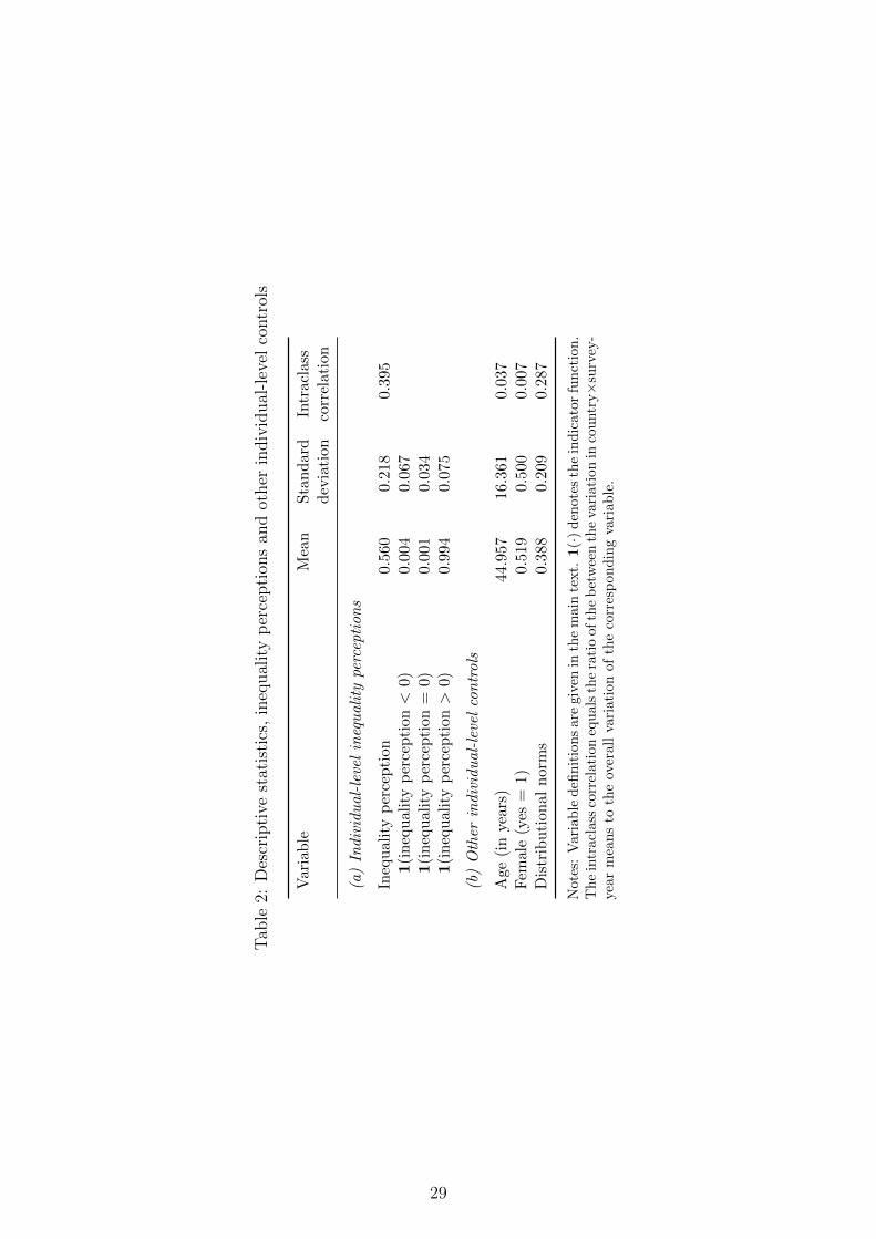
Panel (a) of table 2 presents descriptives for subjective inequality perceptions. In the overall
sample, inequality perceptions average 0.56 Gini points with a standard deviation of about
0.218 (remember that inequality perceptions can, in principle, be interpreted the same way as
a conventional Gini coefficient).
Table 2
The table also shows that very few individuals (less than one percent of the overall sample)
perceive no wage differentials across the different occupations at all, resulting in Gactuali being
exactly equal to zero.10 More important for the empirical analysis, however, note that there
is huge variation in individual perceptions of wage inequality. This quite clearly shows that
individuals really do have widely different perceptions of wage inequality, consistent with the
10Somewhat counterintuitively, the table also shows that there are a few observations with negative inequalityperceptions. This results if an individual reverses the rank ordering of the occupations (with respect to theirwages) for which subjective wage estimates are available, and which are used to construct individual-levelinequality perceptions. Kuhn (2011) provides a more detailed discussion of this issue.
12
literature mentioned in the introduction. This in turn implies that there might be large discrep-
ancies between the effective level of inequality and the level of inequality individuals perceive.11
At the same time, the high intraclass correlation (about 0.395) suggests that inequality per-
ceptions are quite strongly correlated with each other within country×year cells. Thus, there
appear to be large differences in country averages of individual-level inequality perceptions,
reflecting not only differences in the true level of inequality, but also differences in, for example,
the way and intensity the issue of inequality is treated in the media.
3.3 Other Individual-level Controls
Panel (b) of table 2 shows descriptives for the other three individual-level controls used in the
analysis below. The descriptives of age and gender are as expected, with a mean age of about
45 years and slightly more women than men in the sample. More interestingly, note how small
the intraclass correlation for these two variables is – compared to inequality perceptions.
Finally, descriptives for distributional norms reveal, not surprisingly, that the legitimate
level of wage inequality is considerably smaller than the perceived level. Also, the correspond-
ing intraclass correlation shows that distributional norms are less strongly correlated within
country×survey-year than inequality perceptions.
4 Empirical Framework
4.1 Baseline Estimates
To quantify the effect of inequality perceptions on individuals’ attitudes to social inequality, I
will estimate the parameters of a series of regression models that all share the following basic
form:
yit = α + βGactual
it + γxit + ψj[i]t + εit, (1)
with yit denoting attitudes to social inequality of individual i living in country j and having
participated in the survey in year t, and with Gactualit denoting an individual’s perceived level of
11This, of course, also implies that there may be research contexts where simply working with objective dataon inequality, instead of inequality perceptions, might be misleading.
13
wage inequality in his or her country of residence. β is the parameter of primary interest because
it quantifies, under appropriate specifications of the model, the partial effect of inequality
perceptions on individuals’ attitudes to social inequality (oviously, I expect β > 0).
Furthermore, all of the specifications shown below include a full set of country×survey-
year fixed effects, denoted by ψj[i]t in the equation above. The fixed effects will pick up any
systematic differences across countries and years, even if not directly observable in the data at
hand. Most importantly, perhaps, note that the inclusion of these fixed effects will net out any
existing differences across countries and time in the objective, aggregate level of wage inequality.
Moreover, most of the regression specifications shown below will add a few individual-level
control variables, denoted by xit in equation (1). Because most of the available controls at the
individual level are potentially endogenous in the current context, however, I will only include
few such controls; namely: age, gender, and distributional norms.12 A second, more practical
but no less important issue is the fact that there is a considerable amount of missing information
with respect to many of these potential controls (due to both nonresponse and, again, to the
fact that many potentially interesting controls do not appear consistently in all four rounds
of the survey). Thus, the inclusion of additional controls would also lead to an often much
smaller, and potentially very selective, subsample available for the empirical analysis.13
That said, there is of course a similar concern with inequality perceptions and distributional
norms being endogenous as well. This concern is more difficult to deal with empirically, and it
is therefore held back until section 4.3 below.
4.2 Stacking the Data to Estimate Average Effects within Groups
of Similar Items
With a total of forty-nine distinct survey items, there are almost too many potentially inter-
esting outcome variables. It is therefore desirable to have a succinct way to estimate some kind
12In other words, most potential control variables at the individual level are suspect of being influenced byinequality perceptions, implying that specifications including these variables as controls would potentially biasthe estimate of parameter β (i.e. these variables probably constitute “bad controls” in the language of Angristand Pischke, 2008). For example, one can imagine that individuals who have been socialized to have a strongbelief in non-meritocratic principles might choose a different educational track or occupation than those whobelieve that these mechanisms are not very important.
13Nonetheless, appendix table A.3 shows a few selected estimates based on a larger set of individual-levelcontrols. Reassuringly, the comparison shows that the inclusion of additional controls does not have a largeimpact on the interesting parameter estimates.
14
of average effects across items that focus on the same broader conceptual issue.
For this reason, I will focus, for most of the items considered in the empirical analysis, on
estimates that rely on data stacked across several survey items rather than reporting estimates
for single items. In the case where the estimation is based on stacked data, I thus focus on
parameter estimates derived from a regression model with a slightly different structure:
yict = α + βGactual
it + γxit + ψj[i]t + εict, (2)
with yict denoting outcome y of individual i in year t and for item c belonging to some larger
group of related items c = 1, . . . , C; with the total number of items C being larger than one
(if there is only a single item, we are back to equation (1)). A first thing to note is that this
procedure would – if all the items grouped together were available for exactly the same set of
observations – scale up the original sample size by a factor exactly equal to the number of items
grouped together.14 However, in practice, because most of the items considered in the analysis
do not appear in all four years of the survey (less than a quarter of all the items considered),
because items appear in different rounds of the survey, and because of different nonresponse
patterns across items, items which appear in more rounds of the survey will implicitly be given
more weight than those that appear in fewer rounds (a similar argument applies to differences
in the number of observations due to potentially different nonresponse patterns). The fact that
relatively few items are observed in all four rounds of the survey is also the main reason why I
cannot simply use average outcomes as the dependent variable – which would otherwise be the
more natural way of aggregating several items together.
In those specifications where several items are stacked together in the way described above,
I report standard errors clustered by individual to take the fact that the data contain repeated
observations from the same person into account. At the same time, clustered standard errors
will also correct for the inflation of the sample size due to stacking various outcomes from the
same individuals (note that observations for different outcomes but the same individual have
exactly the same values on all the regressors).15
14For example, if there were three (i.e. C = 3) survey questions relating to the same conceptual subject, andif all three items were observed for exactly the same set of observations, then stacking the data would result ina sample exactly three times as large as the original sample size.
15In fact, if the items were perfectly correlated with each other within any given individual, then this procedurewould simply duplicate the information already available in the original data. This would mechanically deflate
15
The main practical advantage of this procedure is that it allows me to reduce the dimension-
ality of the data at hand considerably. Specifically, instead of reporting estimates for each of
the 49 distinct items listed in table 1, the results reported below focus on 14 different outcomes
only (these outcomes mostly represent groups of items or, in a few exceptional cases, single
items).
4.3 Two-Stage Least Squares Estimates
One additional concern with simple OLS estimates of β based on equation (1) is the potential
endogeneity of inequality perceptions due to attitudes about social inequality and inequality
perceptions being determined simultaneously. Thus, in estimating the effect of inequality per-
ceptions on attitudes, ideally one has to net out the potential reverse effect, running from
attitudes to inequality perceptions.
To account for this potentially relevant issue, I will also present two-stage least squares
(2SLS) estimates of the effect of inequality perceptions on individuals’ attitudes to social in-
equality. I will use region-within-country means of subjective inequality perceptions as instru-
ment for an individual’s inequality perceptions.16 The main argument underlying this instru-
ment is that individual inequality perceptions are most likely influenced by the perceptions of
people around them, such as their colleagues at work, their neighbors, or their relatives. At the
same time, individual-level perceptions arguably have a negligible effect on mean perceptions in
a given region. Even though somewhat less obvious, it might also be reasonable to assume that
mean inequality perceptions have no direct effect on individual attitudes to social inequality.17
The associated first-stage regression thus takes the following basic form:
Gactual
it = π0 + π1Gactual
k[i]t + π2xit + ψj[i]t + εi, (3)
conventional standard errors, but standard errors clustered by individual would take properly account of thisissue.
16Dustmann and Preston (2001), for example, propose a similar logic for using an instrument at a higher levelof spatial aggregation in their study on the effect of immigrants inflows on natives’ attitudes to immigration.
17That is, it is implicitly assumed that the instrument has only an indirect effect on the endogenous variable.In the context here, this assumption implies that region-within-country means of inequality perceptions haveno direct effect on the outcome(s) other than through their effect on individual-level inequality perceptions.One potential concern with the specific instrument proposed here is that variation in the instrument might alsoreflect regional differences in the effective level of inequality (which are otherwise not taken into account in theanalysis). In that case, the 2SLS estimates are likely to overestimate the effect of inequality perceptions onattitudes.
16
with Gactualit denoting individual-level perceptions of inequality, and with G
actual
k[i]t denoting mean
inequality perceptions in region-within-country k and survey-year t, which is used as instrument
for individual-level inequality perceptions. The remaining regressors in equation (3) are the
same as those discussed in the context of equation (1) above. Specifically, note that it is still
possible to control for country fixed-effects because there is within-country variation in the
instrument (i.e. K > J). As usual, π1 and its associated standard error are informative about
the strength of the instrument, and the tables below will report the F-statistic associated with
the null hypothesis that the instrument has no partial effect on the endogenous variable.
5 Results
5.1 Beliefs about the Causes of Economic Success
The first set of estimates, shown in table 3, relates to individuals’ beliefs about the causes
of economic success, and I start with the results for individuals’ beliefs about the reasons for
getting ahead. In this and the following two tables, all estimates are based on groups of several
survey items, as discussed in section 4.1 above (the exact number of items which are grouped
together is noted in the bottom of each table).
Table 3
The first five columns report estimates of the partial effect of inequality perceptions on
people’s belief that non-meritocratic mechanisms are important in determining individuals’
wages. The following five columns report analogous estimates related to individuals’ beliefs
that meritocratic mechanisms determine differences in pay. In each of the two panels, the first
three columns report OLS estimates, while the remaining two columns show the corresponding
2SLS estimates. For each point estimate reported (in this and all of the following tables), I
also present (in brackets) an estimate of the approximate elasticity, evaluated at mean values,
of the respective outcome measure with respect to individual-level inequality perceptions.
The estimate reported in the first column of table 3 is from a regression which includes
the full set of country×survey-year fixed effects but no other controls. This first specification
yields a positive and highly significant point estimate, implying that a higher perceived level of
17
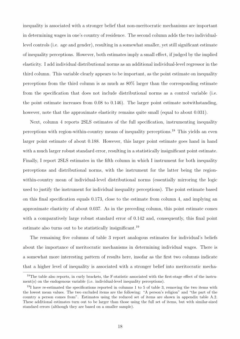
inequality is associated with a stronger belief that non-meritocratic mechanisms are important
in determining wages in one’s country of residence. The second column adds the two individual-
level controls (i.e. age and gender), resulting in a somewhat smaller, yet still significant estimate
of inequality perceptions. However, both estimates imply a small effect, if judged by the implied
elasticity. I add individual distributional norms as an additional individual-level regressor in the
third column. This variable clearly appears to be important, as the point estimate on inequality
perceptions from the third column is as much as 80% larger than the corresponding estimate
from the specification that does not include distributional norms as a control variable (i.e.
the point estimate increases from 0.08 to 0.146). The larger point estimate notwithstanding,
however, note that the approximate elasticity remains quite small (equal to about 0.031).
Next, column 4 reports 2SLS estimates of the full specification, instrumenting inequality
perceptions with region-within-country means of inequality perceptions.18 This yields an even
larger point estimate of about 0.188. However, this larger point estimate goes hand in hand
with a much larger robust standard error, resulting in a statistically insignificant point estimate.
Finally, I report 2SLS estimates in the fifth column in which I instrument for both inequality
perceptions and distributional norms, with the instrument for the latter being the region-
within-country mean of individual-level distributional norms (essentially mirroring the logic
used to justify the instrument for individual inequality perceptions). The point estimate based
on this final specification equals 0.173, close to the estimate from column 4, and implying an
approximate elasticity of about 0.037. As in the preceding column, this point estimate comes
with a comparatively large robust standard error of 0.142 and, consequently, this final point
estimate also turns out to be statistically insignificant.19
The remaining five columns of table 3 report analogous estimates for individual’s beliefs
about the importance of meritocratic mechanisms in determining individual wages. There is
a somewhat more interesting pattern of results here, insofar as the first two columns indicate
that a higher level of inequality is associated with a stronger belief into meritocratic mecha-
18The table also reports, in curly brackets, the F-statistic associated with the first-stage effect of the instru-ment(s) on the endogenous variable (i.e. individual-level inequality perceptions).
19I have re-estimated the specifications reported in columns 1 to 5 of table 3, removing the two items withthe lowest mean values. The two excluded items are the following: “A person’s religion” and “the part of thecountry a person comes from”. Estimates using the reduced set of items are shown in appendix table A.2.These additional estimates turn out to be larger than those using the full set of items, but with similar-sizedstandard errors (although they are based on a smaller sample).
18
nisms being important in determining individual pay, while the remaining three columns (which
include distributional norms as a control) indicate that higher inequality perceptions induce
a weaker belief into the importance of meritocratic mechanisms. Thus, the more demanding
specifications point to a negative, though rather weak effect (implied elasticity of about -0.039
to -0.036) of inequality perceptions on the belief that meritocratic principles are important in
determining pay.
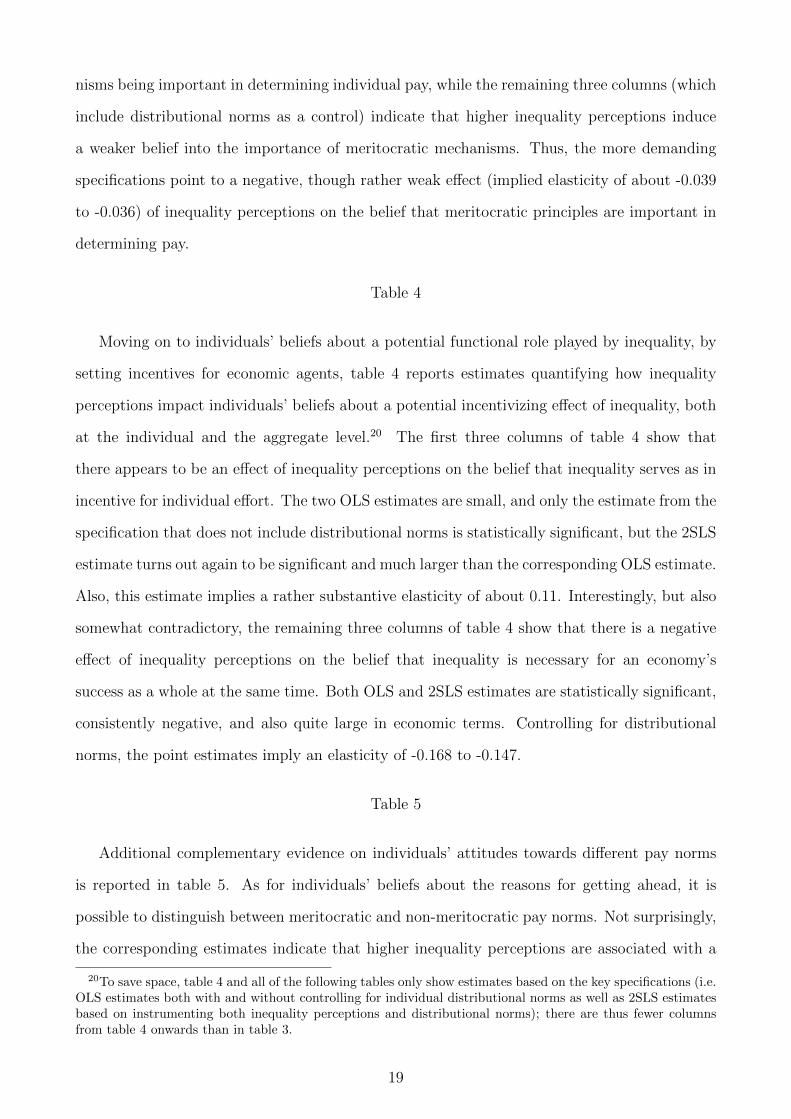
Table 4
Moving on to individuals’ beliefs about a potential functional role played by inequality, by
setting incentives for economic agents, table 4 reports estimates quantifying how inequality
perceptions impact individuals’ beliefs about a potential incentivizing effect of inequality, both
at the individual and the aggregate level.20 The first three columns of table 4 show that
there appears to be an effect of inequality perceptions on the belief that inequality serves as in
incentive for individual effort. The two OLS estimates are small, and only the estimate from the
specification that does not include distributional norms is statistically significant, but the 2SLS
estimate turns out again to be significant and much larger than the corresponding OLS estimate.
Also, this estimate implies a rather substantive elasticity of about 0.11. Interestingly, but also
somewhat contradictory, the remaining three columns of table 4 show that there is a negative
effect of inequality perceptions on the belief that inequality is necessary for an economy’s
success as a whole at the same time. Both OLS and 2SLS estimates are statistically significant,
consistently negative, and also quite large in economic terms. Controlling for distributional
norms, the point estimates imply an elasticity of -0.168 to -0.147.
Table 5
Additional complementary evidence on individuals’ attitudes towards different pay norms
is reported in table 5. As for individuals’ beliefs about the reasons for getting ahead, it is
possible to distinguish between meritocratic and non-meritocratic pay norms. Not surprisingly,
the corresponding estimates indicate that higher inequality perceptions are associated with a
20To save space, table 4 and all of the following tables only show estimates based on the key specifications (i.e.OLS estimates both with and without controlling for individual distributional norms as well as 2SLS estimatesbased on instrumenting both inequality perceptions and distributional norms); there are thus fewer columnsfrom table 4 onwards than in table 3.
19
stronger belief in non-meritocratic pay norms, at least when distributional norms are held con-
stant (note that the relevant OLS estimate switches its sign in this case, depending on whether
distributional norms are held constant or not). Conditional on the inclusion of distributional
norms, however, OLS and 2SLS estimates again appear consistent with each other (and again,
2SLS estimates turn out considerably larger than their OLS counterparts). Including distri-
butional norms as a control variable also makes a difference regarding the effect of inequality
perceptions on meritocratic pay norms. While the OLS estimate for the simpler specification
turns out positive, it becomes negative once distributional norms are also taken into account.
Moreover, note that OLS and 2SLS estimates appear inconsistent in this case, with the OLS es-
timate suggesting a negative effect, and the corresponding 2SLS estimate pointing to a positive
effect of inequality perceptions on the importance of meritocratic pay norms.
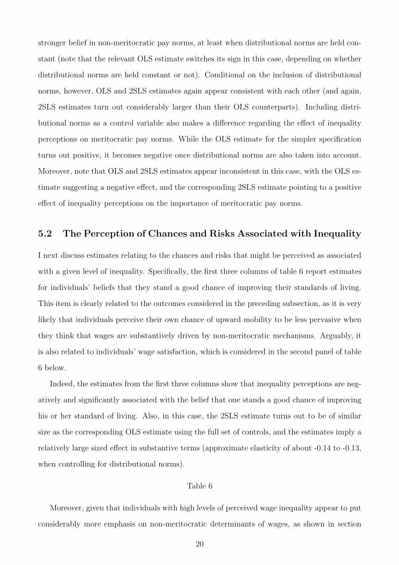
5.2 The Perception of Chances and Risks Associated with Inequality
I next discuss estimates relating to the chances and risks that might be perceived as associated
with a given level of inequality. Specifically, the first three columns of table 6 report estimates
for individuals’ beliefs that they stand a good chance of improving their standards of living.
This item is clearly related to the outcomes considered in the preceding subsection, as it is very
likely that individuals perceive their own chance of upward mobility to be less pervasive when
they think that wages are substantively driven by non-meritocratic mechanisms. Arguably, it
is also related to individuals’ wage satisfaction, which is considered in the second panel of table
6 below.
Indeed, the estimates from the first three columns show that inequality perceptions are neg-
atively and significantly associated with the belief that one stands a good chance of improving
his or her standard of living. Also, in this case, the 2SLS estimate turns out to be of similar
size as the corresponding OLS estimate using the full set of controls, and the estimates imply a
relatively large sized effect in substantive terms (approximate elasticity of about -0.14 to -0.13,
when controlling for distributional norms).
Table 6
Moreover, given that individuals with high levels of perceived wage inequality appear to put
considerably more emphasis on non-meritocratic determinants of wages, as shown in section
20
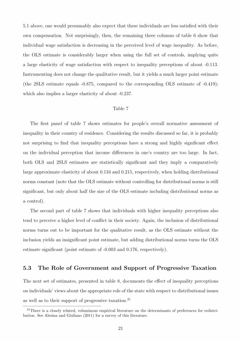
5.1 above, one would presumably also expect that these individuals are less satisfied with their
own compensation. Not surprisingly, then, the remaining three columns of table 6 show that
individual wage satisfaction is decreasing in the perceived level of wage inequality. As before,
the OLS estimate is considerably larger when using the full set of controls, implying quite
a large elasticity of wage satisfaction with respect to inequality perceptions of about -0.113.
Instrumenting does not change the qualitative result, but it yields a much larger point estimate
(the 2SLS estimate equals -0.875, compared to the corresponding OLS estimate of -0.419);
which also implies a larger elasticity of about -0.237.
Table 7
The first panel of table 7 shows estimates for people’s overall normative assessment of
inequality in their country of residence. Considering the results discussed so far, it is probably
not surprising to find that inequality perceptions have a strong and highly significant effect
on the individual perception that income differences in one’s country are too large. In fact,
both OLS and 2SLS estimates are statistically significant and they imply a comparatively
large approximate elasticity of about 0.134 and 0.215, respectively, when holding distributional
norms constant (note that the OLS estimate without controlling for distributional norms is still
significant, but only about half the size of the OLS estimate including distributional norms as
a control).
The second part of table 7 shows that individuals with higher inequality perceptions also
tend to perceive a higher level of conflict in their society. Again, the inclusion of distributional
norms turns out to be important for the qualitative result, as the OLS estimate without the
inclusion yields an insignificant point estimate, but adding distributional norms turns the OLS
estimate significant (point estimate of -0.003 and 0.176, respectively).
5.3 The Role of Government and Support of Progressive Taxation
The next set of estimates, presented in table 8, documents the effect of inequality perceptions
on individuals’ views about the appropriate role of the state with respect to distributional issues
as well as to their support of progressive taxation.21
21There is a closely related, voluminous empirical literature on the determinants of preferences for redistri-bution. See Alesina and Giuliano (2011) for a survey of this literature.
21
Table 8
Consistent with the previous results, the first three columns of table 8 show that a higher
level of perceived inequality is statistically significantly associated with stronger support for
government intervention. That is, people who perceive a high level of wage inequality appear
to be considerably more supportive of intervention by the state. Both OLS and 2SLS estimates
are statistically significant and positive and, again, including distributional norms as a control
yields a much larger OLS estimate and instrumenting yields a still larger point estimate. When
controlling for distributional norms, both OLS and 2SLS estimate imply a relatively large quan-
titative effect of inequality perceptions (as indicated by the comparatively large approximate
elasticity of about 0.097 and 0.188, respectively).
The remaining three columns of table 8 show estimates on individuals’ support of progres-
sive taxation. Again, I find that there is a positive, and statistically highly significant, effect
of inequality perceptions on the support of progressive taxation. The pattern is similar to the
preceding results concerning the role of the state; with the OLS estimate approximately dou-
bling when distributional norms are included as a control, and with a yet higher 2SLS estimate.
Also, the economic size of the estimates is quite large, with an approximate elasticity about
0.11 to about 0.165, depending on the specification.
5.4 Political Preferences and Political Participation
The final set of estimates, reported in table 9, focuses on the effect of inequality perceptions
on individuals’ political preferences as well as their general political participation. The first
three columns of table 9 report estimates for respondents’ identification with the political right
(that is, higher values on the dependent variable signify a stronger identity with the political
right), while the remaining three columns focus on individuals’ more general degree of political
participation, measured by a single item asking about participation at the last election held in
a respondent’s country of residence.
Table 9
Not surprisingly, and consistent with the results presented so far, the first three columns of
table 9 show that higher inequality perceptions are associated with people being significantly
22
less (more) likely to state that they identify with the political right (left). Again, controlling
for individual distributional norms, both OLS and 2SLS estimate imply quite a large effect of
inequality perceptions on political preferences (with an approximate elasticity of about -0.102
and -0.309, respectively).
Finally, the evidence with respect to voting – as a measure of an individual’s general political
participation – is somewhat mixed. The two OLS estimates suggest that political participation
is increasing in an individual’s inequality perception, while the 2SLS estimate turns out to be
small and statistically insignificant. If anything, then, a high perceived level of wage inequality
seems to increase political participation.
6 Conclusions
In this paper, I use a simple yet intuitive empirical measure of individual-level inequality per-
ceptions to estimate how these subjective perceptions affect individuals’ attitudes to and beliefs
about social inequality. Using a broad variety of different outcomes reflecting the diverse di-
mensions of attitudes to social inequality, the empirical analysis shows that a higher level of
perceived wage inequality is statistically significantly associated with a weaker belief into the
proper functioning of (labor) markets. Specifically, I find that individuals who perceive wage
inequality to be high tend to be less (more) likely to believe that wage differentials are driven by
meritocratic (non-meritocratic) principles. Consistent with previous empirical evidence, these
individuals are also less likely to be satisfied with their own compensation from work. Taken
together, these results suggest that a high perceived level of wage inequality has the potential
to undermine the legitimacy of market outcomes. The results are also consistent with the argu-
ment that there is a feedback process running from (the perception of) inequality to attitudes
to social inequality.
I further show that this result is robust to the use of an instrumental-variable estimation
strategy which uses regional means of inequality perceptions as an instrument for individual-
level inequality perceptions. In general, 2SLS estimates turn out to be larger (in absolute
terms) yet mostly consistent with the corresponding OLS estimates. Moreover, the implied
approximate elasticities of attitudes and beliefs with respect to inequality perceptions reveal
that the quantitative size of the estimates effects appear to be plausible. While most of the
23
estimates describing the effect of inequality perceptions on attitudes to social inequality are
statistically significant, most of the corresponding elasticities appear to be small or of moderate
size.
Finally, the results presented in this paper also add to the available empirical evidence
showing that subjective perceptions of economic phenomena shape individuals’ attitudes and
beliefs. The results of this paper show that attitudes to and beliefs about economic inequality
are, in part, influenced by individuals’ perception of the prevailing level of wage inequality in
their country of residence. This in turn implies that changes in inequality might indeed bring
about corresponding changes in attitudes towards social inequality.
24
References
Alesina, A. and Angeletos, G. (2005). Fairness and Redistribution. American Economic Review ,95(3), 960–980.
Alesina, A. and Giuliano, P. (2011). Preferences for Redistribution. In Handbook of SocialEconomics , volume 1A, chapter 4. Elsevier.
Alesina, A., Cozzi, G., and Mantovan, N. (2012). The evolution of ideology, fairness andredistribution. Economic Journal , 122(565), 1244–1261.
Angrist, J. D. and Pischke, J.-S. (2008). Mostly harmless econometrics: An empiricist’s com-panion. Princeton University Press.
Atkinson, A. B. (2008). The changing distribution of earnings in OECD countries . OxfordUniversity Press.
Benabou, R. and Tirole, J. (2006). Belief in a just world and redistributive politics. QuarterlyJournal of Economics , 121(2), 699–746.
Bjørnskov, C., Dreher, A., Fischer, J. A., Schnellenbach, J., and Gehring, K. (2013). Inequalityand happiness: When perceived social mobility and economic reality do not match. Journalof Economic Behavior & Organization, 91, 75–92.
Card, D., Mas, A., Moretti, E., and Saez, E. (2012). Inequality at Work: The Effect of PeerSalaries on Job Satisfaction. American Economic Review , 102(6), 2981–3003.
Chambers, J. R., Swan, L. K., and Heesacker, M. (2014). Better off than we know distortedperceptions of incomes and income inequality in America. Psychological Science, 25(2),613–618.
Charness, G. and Kuhn, P. (2007). Does pay inequality affect worker effort? Experimentalevidence. Journal of Labor Economics , 25(4), 693–723.
Clark, A. and Oswald, A. (1996). Satisfaction and comparison income. Journal of PublicEconomics , 61(3), 359–381.
Clark, A. and Senik, C. (2010). Who compares to whom? The anatomy of income comparisonsin Europe. Economic Journal , 120(544), 573–594.
Clark, A. E., Westergard-Nielsen, N., and Kristensen, N. (2009). Economic satisfaction and in-come rank in small neighbourhoods. Journal of the European Economic Association, 7(2/3),519–527.
Clark, A. E., Masclet, D., and Villeval, M. C. (2010). Effort and comparison income: Experi-mental and survey evidence. Industrial & Labor Relations Review , 63(3), 407–426.
Cornelissen, T., Himmler, O., and Koenig, T. (2011). Perceived unfairness in CEO compensa-tion and work morale. Economics Letters , 110(1), 45–48.
Cruces, G., Truglia, R., and Tetaz, M. (2013). Biased perceptions of income distributionand preferences for redistribution: Evidence from a survey experiment. Journal of PublicEconomics , 98, 100–112.
Di Tella, R., Galiani, S., and Schargrodsky, E. (2007). The formation of beliefs: Evidence fromthe allocation of land titles to squatters. Quarterly Journal of Economics , 122(1), 209–241.
25
Dustmann, C. and Preston, I. (2001). Attitudes to ethnic minorities, ethnic context and locationdecisions. Economic Journal , 111(470), 353–373.
Ferrer-i-Carbonell, A. (2005). Income and well-being: an empirical analysis of the comparisonincome effect. Journal of Public Economics , 89(5-6), 997–1019.
Gemmell, N., Morrissey, O., and Pinar, A. (2004). Tax perceptions and preferences over taxstructure in the United Kingdom. Economic Journal , 114(493), F117–F138.
Giuliano, P. and Spilimbergo, A. (2014). Growing up in a recession. Review of EconomicStudies , 81(2), 787–817.
ISSP Research Group (2014a). International Social Survey Programme: Social Inequality I-IV- ISSP 1987-1992-1999-2009. GESIS Data Archive, Cologne. ZA5890 Data File Version 1.0.0.
ISSP Research Group (2014b). International Social Survey Programme: Social Inequality I-IVadd on - ISSP 1987-1992-1999-2009. GESIS Data Archive, Cologne. ZA5891 Data file Version1.1.0.
Kuhn, A. (2011). In the eye of the beholder: Subjective inequality measures and individuals’assessment of market justice. European Journal of Political Economy , 27(4), 625–641.
Kuziemko, I., Norton, M. I., and Saez, E. (2015). How elastic are preferences for redistribution?evidence from randomized survey experiments. American Economic Review , 105(4), 1478–1508.
Luttmer, E. (2005). Neighbors as Negatives: Relative Earnings and Well-Being. QuarterlyJournal of Economics , 120(3), 963–1002.
Norton, M. and Ariely, D. (2011). Building a better America - one wealth quintile at a time.Perspectives on Psychological Science, 6(1), 9–12.
Olken, B. (2009). Corruption perceptions vs. corruption reality. Journal of Public Economics ,93(7), 950–964.
Osberg, L. and Smeeding, T. (2006). “Fair” inequality? Attitudes toward pay differentials: theUnited States in comparative perspective. American Sociological Review , 71(3), 450–473.
Schneider, S. (2012). Income inequality and its consequences for life satisfaction: What role dosocial cognitions play? Social Indicators Research, 106(3), 419–438.
Schwarze, J. and Harpfer, M. (2007). Are people inequality averse, and do they prefer redistri-bution by the state? Evidence from German longitudinal data on life satisfaction. Journalof Socio-Economics , 36(2), 233–249.
Senik, C. (2005). Income distribution and well-being: what can we learn from subjective data?Journal of Economic Surveys , 19(1), 43–63.
Verme, P. (2011). Life satisfaction and income inequality. Review of Income and Wealth, 57(1),111–127.
Winkelmann, L. and Winkelmann, R. (2010). Does Inequality Harm the Middle Class? Kyklos ,63(2), 301–316.
26
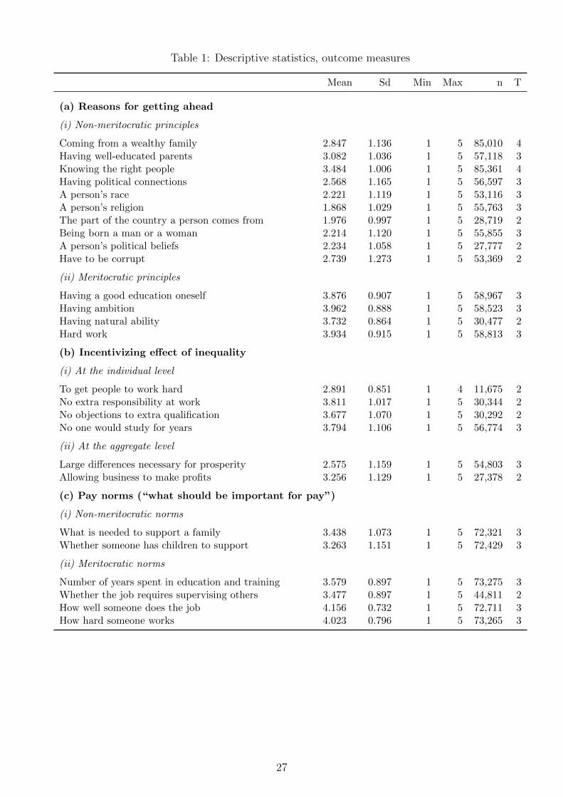
Table 1: Descriptive statistics, outcome measures
Mean Sd Min Max n T
(a) Reasons for getting ahead
(i) Non-meritocratic principles
Coming from a wealthy family 2.847 1.136 1 5 85,010 4Having well-educated parents 3.082 1.036 1 5 57,118 3Knowing the right people 3.484 1.006 1 5 85,361 4Having political connections 2.568 1.165 1 5 56,597 3A person’s race 2.221 1.119 1 5 53,116 3A person’s religion 1.868 1.029 1 5 55,763 3The part of the country a person comes from 1.976 0.997 1 5 28,719 2Being born a man or a woman 2.214 1.120 1 5 55,855 3A person’s political beliefs 2.234 1.058 1 5 27,777 2Have to be corrupt 2.739 1.273 1 5 53,369 2
(ii) Meritocratic principles
Having a good education oneself 3.876 0.907 1 5 58,967 3Having ambition 3.962 0.888 1 5 58,523 3Having natural ability 3.732 0.864 1 5 30,477 2Hard work 3.934 0.915 1 5 58,813 3
(b) Incentivizing effect of inequality
(i) At the individual level
To get people to work hard 2.891 0.851 1 4 11,675 2No extra responsibility at work 3.811 1.017 1 5 30,344 2No objections to extra qualification 3.677 1.070 1 5 30,292 2No one would study for years 3.794 1.106 1 5 56,774 3
(ii) At the aggregate level
Large differences necessary for prosperity 2.575 1.159 1 5 54,803 3Allowing business to make profits 3.256 1.129 1 5 27,378 2
(c) Pay norms (“what should be important for pay”)
(i) Non-meritocratic norms
What is needed to support a family 3.438 1.073 1 5 72,321 3Whether someone has children to support 3.263 1.151 1 5 72,429 3
(ii) Meritocratic norms
Number of years spent in education and training 3.579 0.897 1 5 73,275 3Whether the job requires supervising others 3.477 0.897 1 5 44,811 2How well someone does the job 4.156 0.732 1 5 72,711 3How hard someone works 4.023 0.796 1 5 73,265 3
27
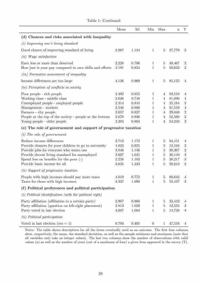
Table 1: Continued
Mean Sd Min Max n T
(d) Chances and risks associated with inequality
(i) Improving one’s living standard
Good chance of improving standard of living 2.987 1.124 1 5 27,779 2
(ii) Wage satisfaction
Earn less or more than deserved 2.228 0.796 1 5 49,467 2How just is your pay compared to own skills and efforts 2.191 0.834 1 5 50,622 2
(iii) Normative assessment of inequality
Income differences are too large 4.126 0.969 1 5 85,125 4
(iv) Perception of conflicts in society
Poor people - rich people 2.492 0.855 1 4 82,510 4Working class - middle class 2.026 0.748 1 4 81,090 4Unemployed people - employed people 2.314 0.844 1 4 25,184 2Management - workers 2.546 0.800 1 4 81,510 4Farmers - city people 2.057 0.827 1 4 29,048 2People at the top of the society - people at the bottom 2.679 0.936 1 4 52,560 2Young people - older people 2.204 0.804 1 4 54,243 3
(e) The role of governement and support of progressive taxation
(i) The role of governement
Reduce income differences 3.710 1.172 1 5 84,151 4Provide chances for poor children to go to university 4.023 0.925 1 5 12,104 2Provide jobs for everyone who wants one 3.846 1.156 1 5 30,367 2Provide decent living standard for unemployed 3.697 1.045 1 5 36,110 3Spend less on benefits for the poor (-) 2.238 1.103 1 5 38,217 3Provide basic income for all 3.635 1.233 1 5 28,613 2
(ii) Support of progressive taxation
People with high incomes should pay more taxes 4.019 0.773 1 5 80,642 4Taxes for those with high incomes 3.337 1.090 1 5 53,107 3
(f) Political preferences and political participation
(i) Political identification (with the political right)
Party affiliation (affiliation to a certain party) 2.907 0.966 1 5 33,442 4Party affiliation (question on left-right placement) 2.813 1.029 1 5 12,555 3Party voted in last election 3.007 1.004 1 5 14,720 4
(ii) Political participation
Voted in last election (yes = 1) 0.794 0.405 0 1 47,516 4
Notes: The table shows descriptives for all the items eventually used as an outcome. The first four columnsshow, respectively, the mean, the standard deviation, as well as the sample minimum and maximum (note thatall variables only take on integer values). The last two columns show the number of observations with validvalues (n) as well as the number of years (out of a maximum of four) a given item appeared in the survey (T).
28
Tab
le2:
Des
crip
tive
stat
isti
cs,
ineq
ual
ity
per
cepti
ons
and
other
indiv
idual
-lev
elco
ntr
ols
Vari
ab
leM
ean
Sta
nd
ard
Intr
acla
ssd
evia
tion
corr
elat
ion
(a)
Indiv
idu
al-
leve
lin
equ
ali
type
rcep
tion
s
Ineq
uali
typ
erce
pti
on0.
560
0.21
80.3
951
(in
equ
alit
yp
erce
pti
on<
0)0.
004
0.06
71
(in
equ
alit
yp
erce
pti
on=
0)0.0
010.
034
1(i
neq
ual
ity
per
cep
tion
>0)
0.99
40.
075
(b)
Oth
erin
div
idu
al-
leve
lco
ntr
ols
Age
(in
year
s)44.9
5716.3
610.0
37F
emale
(yes
=1)
0.51
90.
500
0.0
07D
istr
ibu
tion
aln
orm
s0.3
880.
209
0.2
87
Not
es:
Var
iab
ledefi
nit
ion
sare
giv
enin
the
main
text.
1(·)
den
ote
sth
ein
dic
ato
rfu
nct
ion
.T
he
intr
acla
ssco
rrel
atio
neq
uals
the
rati
oofth
eb
etw
een
the
vari
ati
on
inco
untr
y×
surv
ey-
year
mea
ns
toth
eov
erall
vari
ati
on
of
the
corr
esp
on
din
gva
riab
le.
29
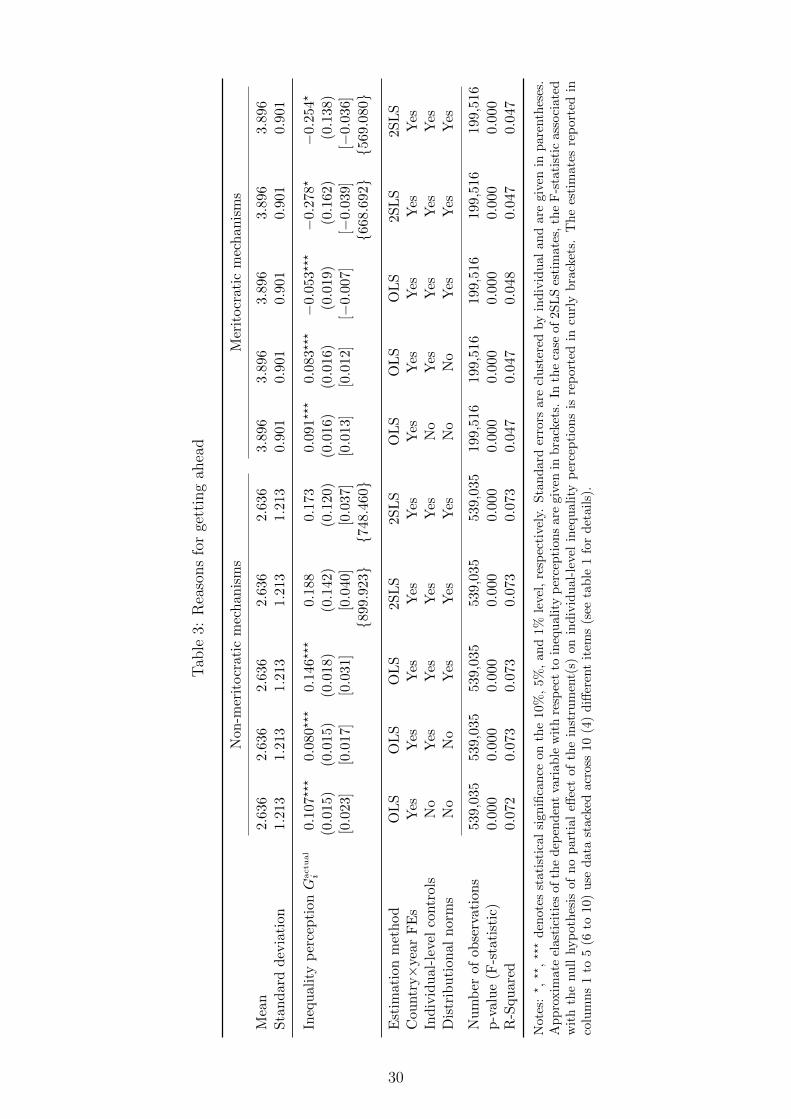
Tab
le3:
Rea
sons
for
gett
ing
ahea
d
Non
-mer
itocr
atic
mec
han
ism
sM
erit
ocr
atic
mec
han
ism
s
Mea
n2.
636
2.63
62.
636
2.63
62.
636
3.89
63.
896
3.8
963.
896
3.89
6S
tan
dard
dev
iati
on1.2
13
1.21
31.
213
1.21
31.
213
0.90
10.
901
0.9
010.
901
0.90
1
Ineq
uali
typ
erce
pti
onG
actu
al
i0.
107???
0.08
0???
0.1
46???
0.18
80.
173
0.09
1???
0.0
83???−
0.0
53???
−0.
278?
−0.2
54?
(0.0
15)
(0.0
15)
(0.0
18)
(0.1
42)
(0.1
20)
(0.0
16)
(0.0
16)
(0.0
19)
(0.1
62)
(0.1
38)
[0.0
23]
[0.0
17]
[0.0
31]
[0.0
40]
[0.0
37]
[0.0
13]
[0.0
12]
[−0.0
07]
[−0.
039]
[−0.0
36]
{899.9
23}
{748.4
60}
{668.6
92}
{569.0
80}
Est
imati
on
met
hod
OL
SO
LS
OL
S2S
LS
2SL
SO
LS
OL
SO
LS
2SL
S2S
LS
Cou
ntr
y×
year
FE
sY
esY
esY
esY
esY
esY
esY
esY
esY
esY
esIn
div
idu
al-
leve
lco
ntr
ols
No
Yes
Yes
Yes
Yes
No
Yes
Yes
Yes
Yes
Dis
trib
uti
on
aln
orm
sN
oN
oY
esY
esY
esN
oN
oY
esY
esY
es
Nu
mb
erof
obse
rvati
on
s539,
035
539
,035
539,
035
539,
035
539,
035
199,
516
199,
516
199,
516
199,
516
199,
516
p-v
alu
e(F
-sta
tist
ic)
0.0
00
0.00
00.
000
0.00
00.
000
0.00
00.
000
0.0
000.
000
0.00
0R
-Squ
ared
0.0
72
0.07
30.
073
0.07
30.
073
0.04
70.
047
0.0
480.
047
0.04
7
Not
es:
?,??,???
den
otes
stat
isti
cal
sign
ifica
nce
onth
e10
%,
5%,
an
d1%
leve
l,re
spec
tive
ly.
Sta
nd
ard
erro
rsare
clu
ster
edby
ind
ivid
ual
an
dare
giv
enin
pare
nth
eses
.A
pp
roxim
ate
elas
tici
ties
ofth
ed
epen
den
tva
riab
lew
ith
resp
ect
toin
equ
ali
typ
erce
pti
on
sare
giv
enin
bra
cket
s.In
the
case
of
2S
LS
esti
mate
s,th
eF
-sta
tist
icass
oci
ate
dw
ith
the
nu
llhyp
oth
esis
ofn
op
arti
aleff
ect
ofth
ein
stru
men
t(s)
on
ind
ivid
ual-
level
ineq
uali
typ
erce
pti
on
sis
rep
ort
edin
curl
yb
rack
ets.
Th
ees
tim
ate
sre
port
edin
colu
mn
s1
to5
(6to
10)
use
dat
ast
acked
acro
ss10
(4)
diff
eren
tit
ems
(see
tab
le1
for
det
ail
s).
30
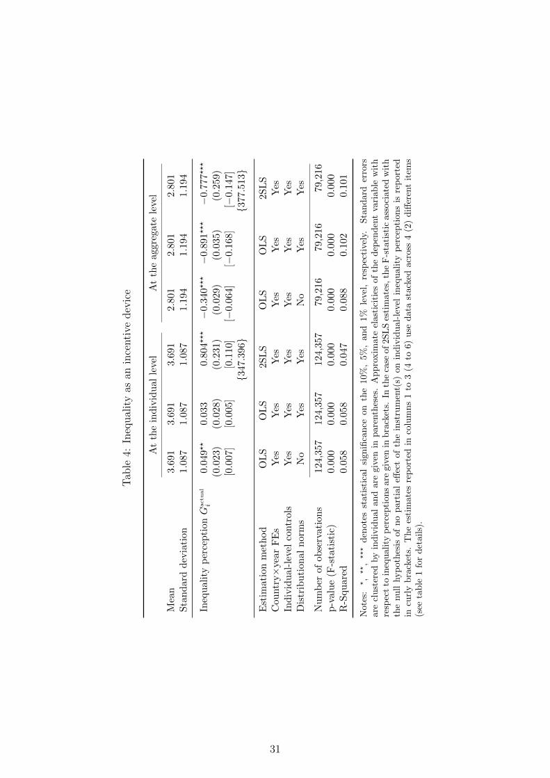
Tab
le4:
Ineq
ual
ity
asan
ince
nti
vedev
ice
At
the
ind
ivid
ual
leve
lA
tth
eag
greg
ate
leve
l
Mea
n3.
691
3.69
13.
691
2.8
012.8
012.
801
Sta
nd
ard
dev
iati
on1.0
871.
087
1.08
71.1
941.1
941.
194
Ineq
uali
typ
erce
pti
onG
actu
al
i0.
049?
?0.0
330.
804???−
0.3
40???−
0.8
91???
−0.
777?
??
(0.0
23)
(0.0
28)
(0.2
31)
(0.0
29)
(0.0
35)
(0.2
59)
[0.0
07]
[0.0
05]
[0.1
10]
[−0.0
64]
[−0.1
68]
[−0.
147]
{347.3
96}
{377.5
13}
Est
imat
ion
met
hod
OL
SO
LS
2SL
SO
LS
OL
S2S
LS
Cou
ntr
y×
year
FE
sY
esY
esY
esY
esY
esY
esIn
div
idu
al-l
evel
contr
ols
Yes
Yes
Yes
Yes
Yes
Yes
Dis
trib
uti
on
al
norm
sN
oY
esY
esN
oY
esY
es
Nu
mb
erof
obse
rvat
ion
s12
4,35
712
4,35
712
4,35
779
,216
79,2
1679
,216
p-v
alu
e(F
-sta
tist
ic)
0.0
000.
000
0.00
00.0
000.0
000.
000
R-S
qu
ared
0.0
580.
058
0.04
70.0
880.1
020.
101
Not
es:
?,
??,
???
den
otes
stat
isti
cal
sign
ifica
nce
on
the
10%
,5%
,an
d1%
leve
l,re
spec
tive
ly.
Sta
nd
ard
erro
rsar
ecl
ust
ered
by
ind
ivid
ual
and
are
giv
enin
pare
nth
eses
.A
pp
roxim
ate
elast
icit
ies
of
the
dep
end
ent
vari
ab
lew
ith
resp
ect
toin
equ
alit
yp
erce
pti
ons
are
giv
enin
bra
cket
s.In
the
case
of
2SL
Ses
tim
ate
s,th
eF
-sta
tist
icass
oci
ate
dw
ith
the
nu
llhyp
oth
esis
ofn
op
arti
aleff
ect
of
the
inst
rum
ent(
s)on
ind
ivid
ual-
leve
lin
equ
ali
typ
erce
pti
on
sis
rep
ort
edin
curl
ybra
cket
s.T
he
esti
mat
esre
port
edin
colu
mn
s1
to3
(4to
6)
use
data
stack
edacr
oss
4(2
)d
iffer
ent
item
s(s
eeta
ble
1fo
rd
etai
ls).
31
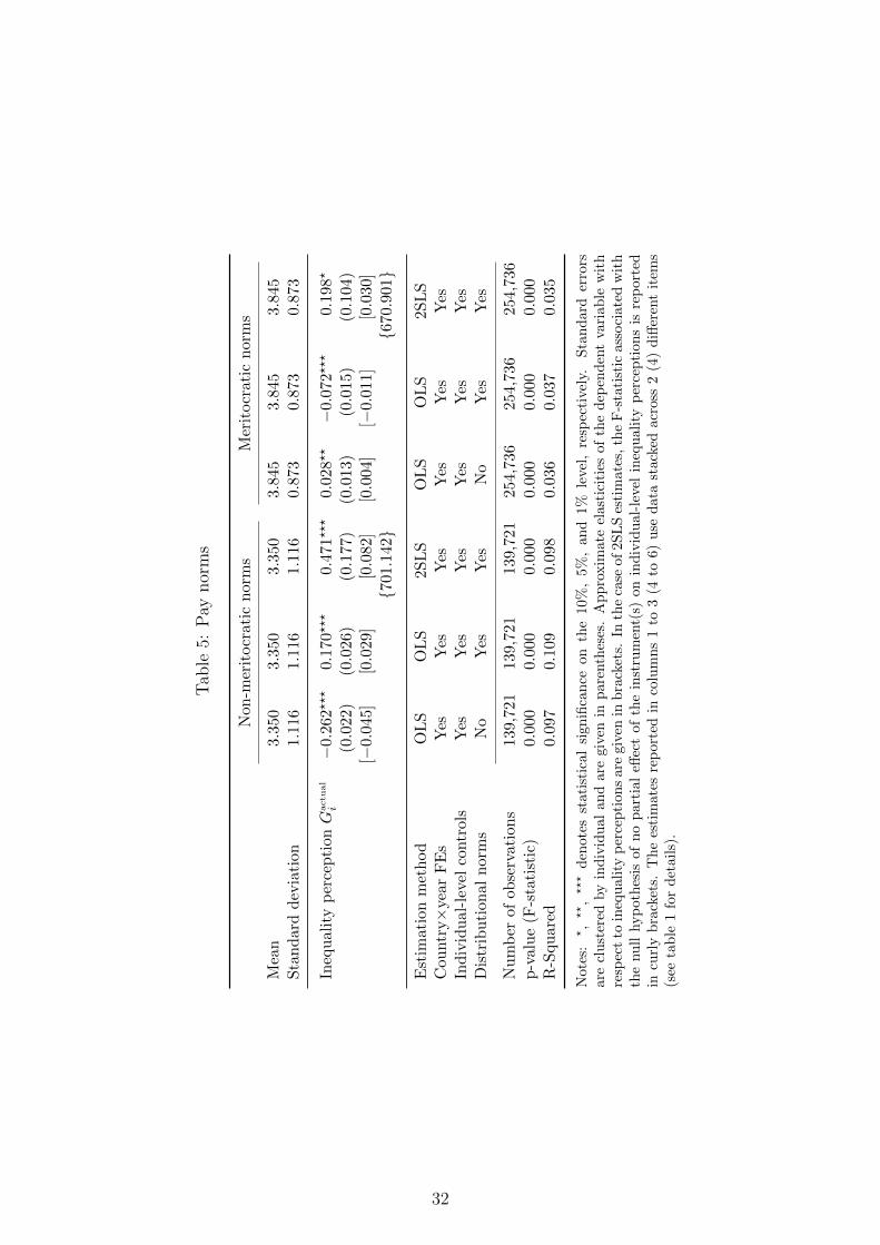
Tab
le5:
Pay
nor
ms
Non
-mer
itocr
atic
nor
ms
Mer
itocr
atic
nor
ms
Mea
n3.3
503.
350
3.35
03.
845
3.8
453.
845
Sta
nd
ard
dev
iati
on1.1
161.
116
1.11
60.
873
0.8
730.
873
Ineq
uali
typ
erce
pti
onG
actu
al
i−
0.26
2???
0.17
0???
0.4
71???
0.02
8??−
0.0
72???
0.19
8?
(0.0
22)
(0.0
26)
(0.1
77)
(0.0
13)
(0.0
15)
(0.1
04)
[−0.
045]
[0.0
29]
[0.0
82]
[0.0
04]
[−0.0
11]
[0.0
30]
{701.1
42}
{670.9
01}
Est
imat
ion
met
hod
OL
SO
LS
2SL
SO
LS
OL
S2S
LS
Cou
ntr
y×
year
FE
sY
esY
esY
esY
esY
esY
esIn
div
idu
al-l
evel
contr
ols
Yes
Yes
Yes
Yes
Yes
Yes
Dis
trib
uti
on
al
norm
sN
oY
esY
esN
oY
esY
es
Nu
mb
erof
obse
rvat
ion
s13
9,72
113
9,72
113
9,72
125
4,73
625
4,73
625
4,73
6p
-valu
e(F
-sta
tist
ic)
0.0
000.
000
0.00
00.
000
0.0
000.
000
R-S
qu
ared
0.09
70.
109
0.09
80.
036
0.0
370.
035
Not
es:
?,
??,
???
den
otes
stat
isti
cal
sign
ifica
nce
on
the
10%
,5%
,an
d1%
leve
l,re
spec
tive
ly.
Sta
nd
ard
erro
rsar
ecl
ust
ered
by
ind
ivid
ual
and
are
giv
enin
pare
nth
eses
.A
pp
roxim
ate
elast
icit
ies
of
the
dep
end
ent
vari
ab
lew
ith
resp
ect
toin
equ
alit
yp
erce
pti
ons
are
giv
enin
bra
cket
s.In
the
case
of
2SL
Ses
tim
ate
s,th
eF
-sta
tist
icass
oci
ate
dw
ith
the
nu
llhyp
oth
esis
ofn
op
arti
aleff
ect
of
the
inst
rum
ent(
s)on
ind
ivid
ual-
leve
lin
equ
ali
typ
erce
pti
on
sis
rep
ort
edin
curl
ybra
cket
s.T
he
esti
mat
esre
port
edin
colu
mn
s1
to3
(4to
6)
use
data
stack
edacr
oss
2(4
)d
iffer
ent
item
s(s
eeta
ble
1fo
rd
etai
ls).
32
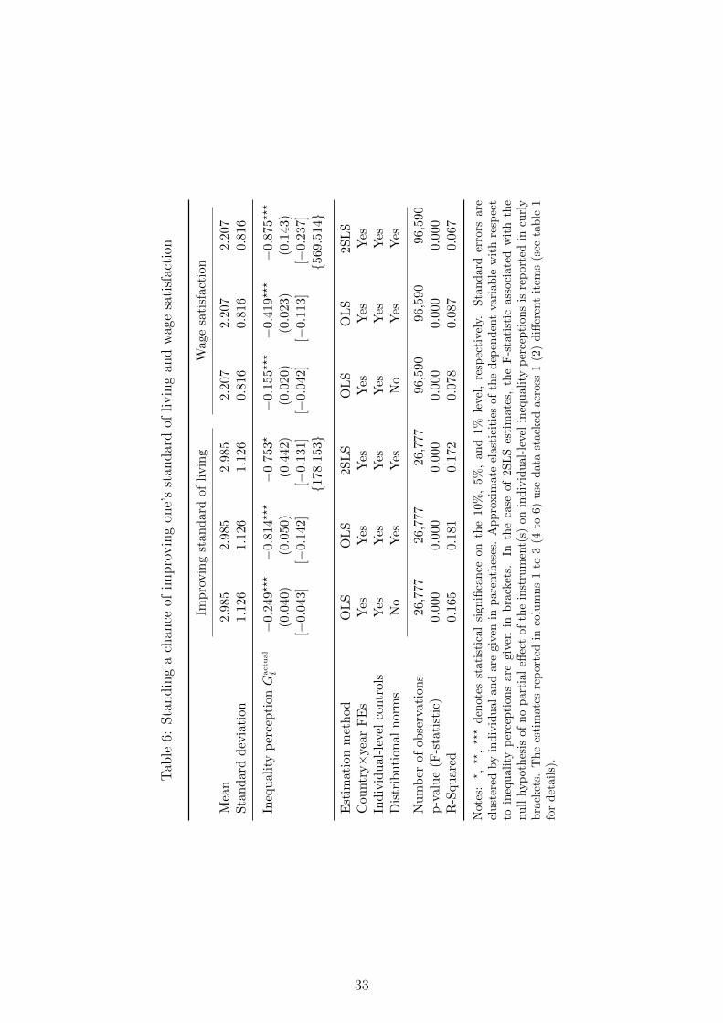
Tab
le6:
Sta
ndin
ga
chan
ceof
impro
vin
gon
e’s
stan
dar
dof
livin
gan
dw
age
sati
sfac
tion
Imp
rovin
gst
and
ard
ofli
vin
gW
age
sati
sfac
tion
Mea
n2.9
852.9
852.
985
2.2
072.2
072.
207
Sta
nd
ard
dev
iati
on1.1
261.1
261.
126
0.8
160.8
160.
816
Ineq
ual
ity
per
cep
tionG
actu
al
i−
0.24
9???−
0.81
4???
−0.7
53?
−0.1
55???−
0.4
19???
−0.
875?
??
(0.0
40)
(0.0
50)
(0.4
42)
(0.0
20)
(0.0
23)
(0.1
43)
[−0.
043]
[−0.
142]
[−0.1
31]
[−0.0
42]
[−0.1
13]
[−0.
237]
{178.1
53}
{569.5
14}
Est
imat
ion
met
hod
OL
SO
LS
2SL
SO
LS
OL
S2S
LS
Cou
ntr
y×
year
FE
sY
esY
esY
esY
esY
esY
esIn
div
idu
al-l
evel
contr
ols
Yes
Yes
Yes
Yes
Yes
Yes
Dis
trib
uti
onal
nor
ms
No
Yes
Yes
No
Yes
Yes
Nu
mb
erof
ob
serv
atio
ns
26,7
7726
,777
26,7
7796
,590
96,5
9096
,590
p-v
alu
e(F
-sta
tist
ic)
0.0
000.0
000.
000
0.0
000.0
000.
000
R-S
qu
ared
0.16
50.1
810.
172
0.0
780.0
870.
067
Not
es:
?,
??,
???
den
otes
stat
isti
cal
sign
ifica
nce
on
the
10%
,5%
,an
d1%
leve
l,re
spec
tive
ly.
Sta
nd
ard
erro
rsare
clu
ster
edby
ind
ivid
ual
and
are
give
nin
pare
nth
eses
.A
pp
roxim
ate
elast
icit
ies
of
the
dep
end
ent
vari
ab
lew
ith
resp
ect
toin
equ
alit
yp
erce
pti
ons
are
give
nin
bra
cket
s.In
the
case
of
2S
LS
esti
mate
s,th
eF
-sta
tist
icass
oci
ate
dw
ith
the
nu
llhyp
oth
esis
ofn
opar
tial
effec
tof
the
inst
rum
ent(
s)on
ind
ivid
ual-
level
ineq
uali
typ
erce
pti
on
sis
rep
ort
edin
curl
yb
rack
ets.
Th
ees
tim
ates
rep
orte
din
colu
mn
s1
to3
(4to
6)
use
data
stack
edacr
oss
1(2
)d
iffer
ent
item
s(s
eeta
ble
1fo
rd
etai
ls).
33
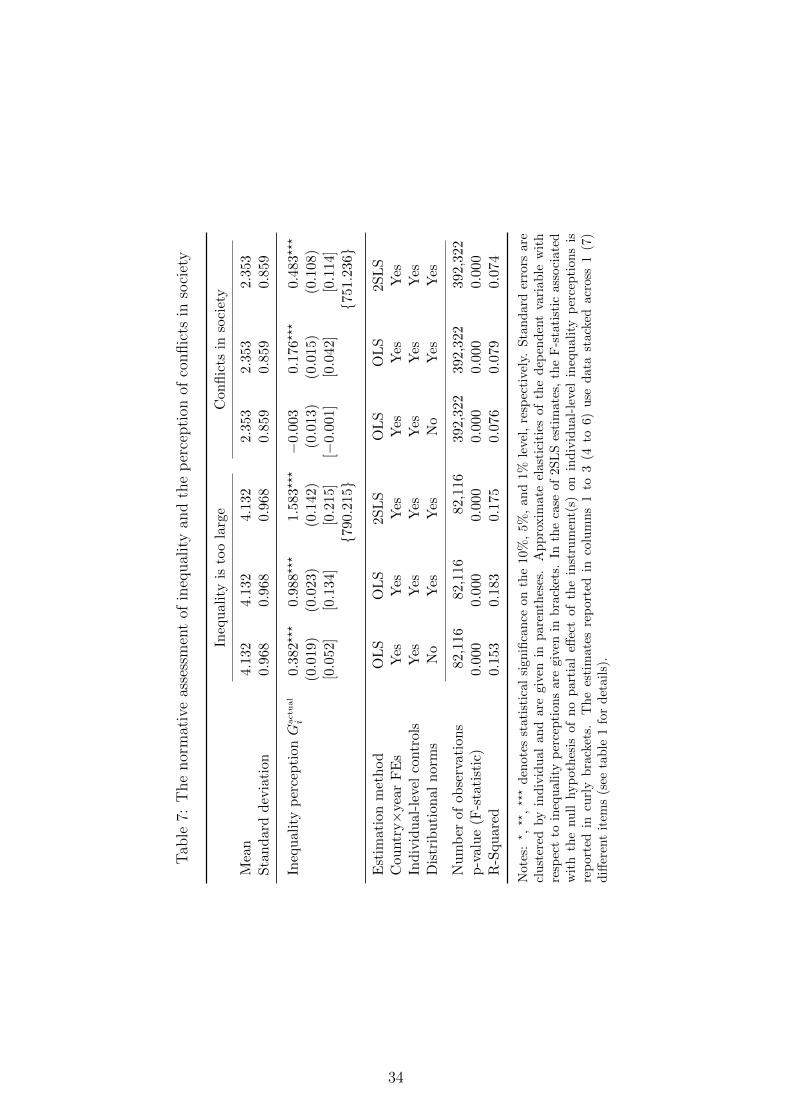
Tab
le7:
The
nor
mat
ive
asse
ssm
ent
ofin
equal
ity
and
the
per
cepti
onof
conflic
tsin
soci
ety
Ineq
ual
ity
isto
ola
rge
Con
flic
tsin
soci
ety
Mea
n4.
132
4.13
24.
132
2.3
532.
353
2.35
3S
tan
dar
dd
evia
tion
0.96
80.
968
0.96
80.8
590.
859
0.85
9
Ineq
uali
typ
erce
pti
onG
actu
al
i0.3
82???
0.9
88???
1.58
3???−
0.00
30.
176???
0.48
3???
(0.0
19)
(0.0
23)
(0.1
42)
(0.0
13)
(0.0
15)
(0.1
08)
[0.0
52]
[0.1
34]
[0.2
15]
[−0.
001]
[0.0
42]
[0.1
14]
{790.2
15}
{751.2
36}
Est
imati
on
met
hod
OL
SO
LS
2SL
SO
LS
OL
S2S
LS
Cou
ntr
y×
year
FE
sY
esY
esY
esY
esY
esY
esIn
div
idu
al-l
evel
contr
ols
Yes
Yes
Yes
Yes
Yes
Yes
Dis
trib
uti
on
al
norm
sN
oY
esY
esN
oY
esY
es
Nu
mb
erof
obse
rvat
ion
s82
,116
82,1
1682
,116
392,
322
392,
322
392,
322
p-v
alu
e(F
-sta
tist
ic)
0.00
00.
000
0.00
00.0
000.
000
0.00
0R
-Squ
ared
0.1
530.
183
0.17
50.0
760.
079
0.07
4
Not
es:
?,??,???
den
otes
stat
isti
cal
sign
ifica
nce
on
the
10%
,5%
,an
d1%
level
,re
spec
tive
ly.
Sta
ndard
erro
rsare
clu
ster
edby
ind
ivid
ual
and
are
give
nin
pare
nth
eses
.A
pp
roxim
ate
elast
icit
ies
of
the
dep
end
ent
vari
ab
lew
ith
resp
ect
toin
equ
alit
yp
erce
pti
ons
are
giv
enin
bra
cket
s.In
the
case
of
2S
LS
esti
mate
s,th
eF
-sta
tist
icass
oci
ate
dw
ith
the
nu
llhyp
oth
esis
ofn
op
arti
al
effec
tof
the
inst
rum
ent(
s)on
ind
ivid
ual-
leve
lin
equ
ali
typ
erce
pti
on
sis
rep
orte
din
curl
yb
rack
ets.
Th
ees
tim
ate
sre
port
edin
colu
mn
s1
to3
(4to
6)
use
data
stack
edacr
oss
1(7
)d
iffer
ent
item
s(s
eeta
ble
1fo
rd
etail
s).
34
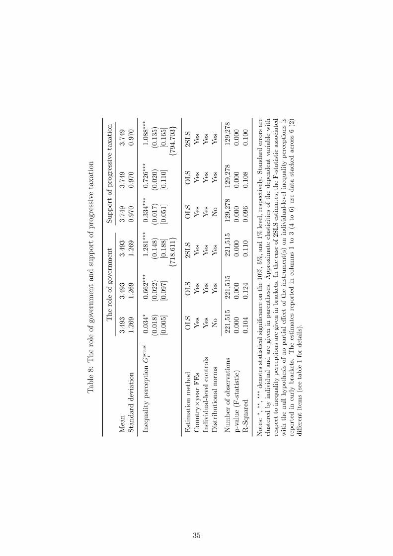
Tab
le8:
The
role
ofgo
vern
men
tan
dsu
pp
ort
ofpro
gres
sive
taxat
ion
Th
ero
leof
gove
rnm
ent
Su
pp
ort
ofp
rogr
essi
veta
xat
ion
Mea
n3.
493
3.49
33.
493
3.74
93.
749
3.74
9S
tan
dar
dd
evia
tion
1.2
691.
269
1.26
90.
970
0.97
00.
970
Ineq
ual
ity
per
cep
tion
Gactu
al
i0.
034?
0.66
2???
1.2
81???
0.33
4???
0.72
6???
1.0
88???
(0.0
18)
(0.0
22)
(0.1
48)
(0.0
17)
(0.0
20)
(0.1
35)
[0.0
05]
[0.0
97]
[0.1
88]
[0.0
51]
[0.1
10]
[0.1
65]
{718.6
11}
{794.7
03}
Est
imati
on
met
hod
OL
SO
LS
2SL
SO
LS
OL
S2S
LS
Cou
ntr
y×
year
FE
sY
esY
esY
esY
esY
esY
esIn
div
idu
al-
leve
lco
ntr
ols
Yes
Yes
Yes
Yes
Yes
Yes
Dis
trib
uti
onal
nor
ms
No
Yes
Yes
No
Yes
Yes
Nu
mb
erof
ob
serv
atio
ns
221,
515
221,
515
221,
515
129,
278
129,
278
129,
278
p-v
alu
e(F
-sta
tist
ic)
0.0
000.
000
0.00
00.
000
0.00
00.
000
R-S
qu
ared
0.1
040.
124
0.11
00.
096
0.10
80.
100
Not
es:
?,??,???
den
otes
stat
isti
cal
sign
ifica
nce
on
the
10%
,5%
,an
d1%
leve
l,re
spec
tivel
y.S
tan
dard
erro
rsare
clu
ster
edby
indiv
idu
alan
dar
egi
ven
inp
are
nth
eses
.A
pp
roxim
ate
elast
icit
ies
of
the
dep
end
ent
vari
ab
lew
ith
resp
ect
toin
equal
ity
per
cep
tion
sar
egiv
enin
bra
cket
s.In
the
case
of
2S
LS
esti
mate
s,th
eF
-sta
tist
icass
oci
ate
dw
ith
the
nu
llhyp
oth
esis
ofn
op
arti
al
effec
tof
the
inst
rum
ent(
s)on
ind
ivid
ual-
leve
lin
equ
ali
typ
erce
pti
on
sis
rep
orte
din
curl
yb
rack
ets.
Th
ees
tim
ate
sre
port
edin
colu
mn
s1
to3
(4to
6)
use
data
stack
edacr
oss
6(2
)d
iffer
ent
item
s(s
eeta
ble
1fo
rd
etail
s).
35
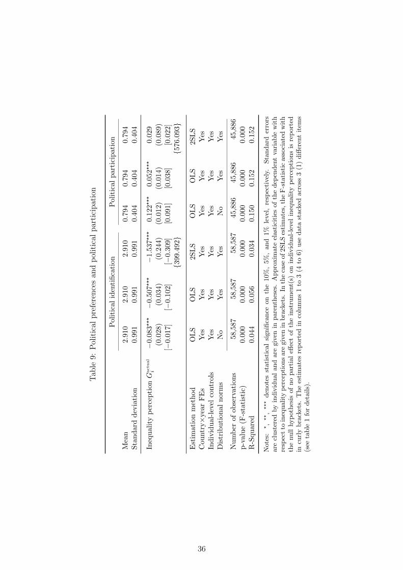
Tab
le9:
Pol
itic
alpre
fere
nce
san
dp
olit
ical
par
tici
pat
ion
Pol
itic
alid
enti
fica
tion
Pol
itic
alp
arti
cip
atio
n
Mea
n2.9
102.9
102.9
100.
794
0.79
40.
794
Sta
nd
ard
dev
iati
on
0.9
910.9
910.9
910.
404
0.40
40.
404
Ineq
uali
typ
erce
pti
onG
actu
al
i−
0.0
83???−
0.5
07???
−1.5
37???
0.1
22???
0.05
2???
0.0
29(0.0
28)
(0.0
34)
(0.2
44)
(0.0
12)
(0.0
14)
(0.0
89)
[−0.0
17]
[−0.1
02]
[−0.3
09]
[0.0
91]
[0.0
38]
[0.0
22]
{399.4
92}
{576.0
93}
Est
imat
ion
met
hod
OL
SO
LS
2SL
SO
LS
OL
S2S
LS
Cou
ntr
y×
year
FE
sY
esY
esY
esY
esY
esY
esIn
div
idu
al-l
evel
contr
ols
Yes
Yes
Yes
Yes
Yes
Yes
Dis
trib
uti
on
al
norm
sN
oY
esY
esN
oY
esY
es
Nu
mb
erof
obse
rvat
ion
s58
,587
58,5
8758
,587
45,8
8645
,886
45,8
86p
-valu
e(F
-sta
tist
ic)
0.0
000.0
000.0
000.
000
0.00
00.
000
R-S
qu
are
d0.
044
0.0
560.0
340.
150
0.15
20.
152
Not
es:
?,
??,
???
den
otes
stat
isti
cal
sign
ifica
nce
on
the
10%
,5%
,an
d1%
leve
l,re
spec
tive
ly.
Sta
nd
ard
erro
rsar
ecl
ust
ered
by
ind
ivid
ual
and
are
giv
enin
pare
nth
eses
.A
pp
roxim
ate
elast
icit
ies
of
the
dep
end
ent
vari
ab
lew
ith
resp
ect
toin
equ
alit
yp
erce
pti
ons
are
giv
enin
bra
cket
s.In
the
case
of
2SL
Ses
tim
ate
s,th
eF
-sta
tist
icass
oci
ate
dw
ith
the
nu
llhyp
oth
esis
ofn
op
arti
aleff
ect
of
the
inst
rum
ent(
s)on
ind
ivid
ual-
leve
lin
equ
ali
typ
erce
pti
on
sis
rep
ort
edin
curl
ybra
cket
s.T
he
esti
mat
esre
port
edin
colu
mn
s1
to3
(4to
6)
use
data
stack
edacr
oss
3(1
)d
iffer
ent
item
s(s
eeta
ble
1fo
rd
etai
ls).
36
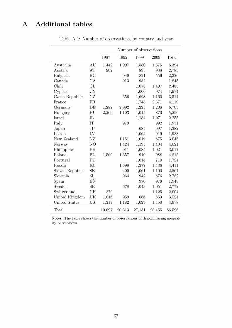
A Additional tables
Table A.1: Number of observations, by country and year
Number of observations
1987 1992 1999 2009 Total
Australia AU 1,442 1,997 1,580 1,375 6,394Austria AT 902 895 988 2,785Bulgaria BG 949 821 556 2,326Canada CA 913 932 1,845Chile CL 1,078 1,407 2,485Cyprus CY 1,000 974 1,974Czech Republic CZ 656 1,698 1,160 3,514France FR 1,748 2,371 4,119Germany DE 1,282 2,992 1,223 1,208 6,705Hungary HU 2,269 1,103 1,014 870 5,256Israel IL 1,184 1,071 2,255Italy IT 979 992 1,971Japan JP 685 697 1,382Latvia LV 1,064 919 1,983New Zealand NZ 1,151 1,019 875 3,045Norway NO 1,424 1,193 1,404 4,021Philippines PH 911 1,085 1,021 3,017Poland PL 1,560 1,357 910 988 4,815Portugal PT 1,014 710 1,724Russia RU 1,698 1,277 1,436 4,411Slovak Republic SK 400 1,061 1,100 2,561Slovenia SI 964 942 876 2,782Spain ES 970 978 1,948Sweden SE 678 1,043 1,051 2,772Switzerland CH 879 1,125 2,004United Kingdom UK 1,046 959 666 853 3,524United States US 1,317 1,182 1,029 1,450 4,978
Total 10,697 20,313 27,131 28,455 86,596
Notes: The table shows the number of observations with nonmissing inequal-ity perceptions.
37
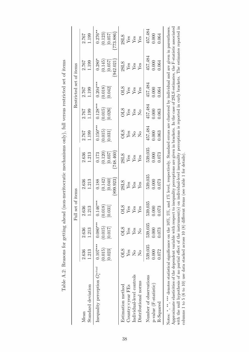
Tab
leA
.2:
Rea
sons
for
gett
ing
ahea
d(n
on-m
erit
ocr
atic
mec
han
ism
son
ly),
full
vers
us
rest
rict
edse
tof
item
s
Fu
llse
tof
item
sR
estr
icte
dse
tof
item
s
Mea
n2.
636
2.63
62.
636
2.63
62.
636
2.76
72.
767
2.76
72.
767
2.76
7S
tan
dard
dev
iati
on1.2
13
1.21
31.
213
1.21
31.
213
1.19
91.
199
1.19
91.
199
1.19
9
Ineq
ual
ity
per
cep
tion
Gactu
al
i0.
107?
??
0.0
80???
0.1
46???
0.18
80.
173
0.15
0???
0.12
8???
0.20
4???
0.2
80?
0.27
6??
(0.0
15)
(0.0
15)
(0.0
18)
(0.1
42)
(0.1
20)
(0.0
15)
(0.0
15)
(0.0
18)
(0.1
45)
(0.1
23)
[0.0
23]
[0.0
17]
[0.0
31]
[0.0
40]
[0.0
37]
[0.0
31]
[0.0
26]
[0.0
42]
[0.0
57]
[0.0
57]
{899.9
23}
{748.4
60}
{942.0
21}
{773.8
86}
Est
imati
on
met
hod
OL
SO
LS
OL
S2S
LS
2SL
SO
LS
OL
SO
LS
2SL
S2S
LS
Cou
ntr
y×
year
FE
sY
esY
esY
esY
esY
esY
esY
esY
esY
esY
esIn
div
idu
al-
leve
lco
ntr
ols
No
Yes
Yes
Yes
Yes
No
Yes
Yes
Yes
Yes
Dis
trib
uti
onal
nor
ms
No
No
Yes
Yes
Yes
No
No
Yes
Yes
Yes
Nu
mb
erof
ob
serv
ati
on
s53
9,0
3553
9,03
553
9,03
553
9,03
553
9,03
545
7,48
445
7,48
445
7,48
445
7,48
445
7,48
4p
-val
ue
(F-s
tati
stic
)0.0
00
0.00
00.
000
0.00
00.
000
0.00
00.
000
0.00
00.
000
0.00
0R
-Squ
ared
0.0
72
0.07
30.
073
0.07
30.
073
0.06
30.
063
0.06
40.
064
0.06
4
Not
es:
?,??,???
den
otes
stat
isti
cal
sign
ifica
nce
onth
e10
%,
5%
,an
d1%
leve
l,re
spec
tive
ly.
Sta
nd
ard
erro
rsare
clu
ster
edby
ind
ivid
ual
an
dare
giv
enin
pare
nth
eses
.A
pp
roxim
ate
elas
tici
ties
ofth
ed
epen
den
tva
riab
lew
ith
resp
ect
toin
equ
ali
typ
erce
pti
on
sare
giv
enin
bra
cket
s.In
the
case
of
2S
LS
esti
mate
s,th
eF
-sta
tist
icass
oci
ate
dw
ith
the
nu
llhyp
oth
esis
ofn
op
arti
aleff
ect
ofth
ein
stru
men
t(s)
on
ind
ivid
ual-
leve
lin
equ
ali
typ
erce
pti
on
sis
rep
ort
edin
curl
yb
rack
ets.
Th
ees
tim
ate
sre
port
edin
colu
mn
s1
to5
(6to
10)
use
dat
ast
acked
acro
ss10
(8)
diff
eren
tit
ems
(see
tab
le1
for
det
ail
s).
38
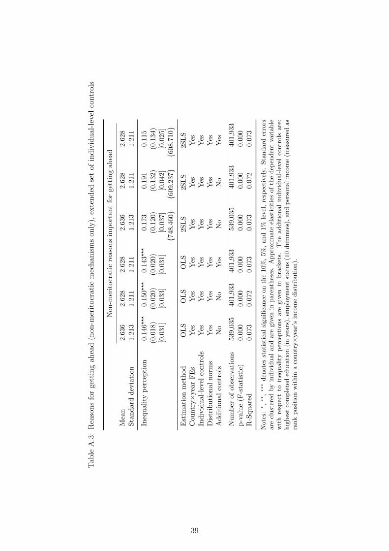
Tab
leA
.3:
Rea
sons
for
gett
ing
ahea
d(n
on-m
erit
ocr
atic
mec
han
ism
son
ly),
exte
nded
set
ofin
div
idual
-lev
elco
ntr
ols
Non
-mer
itocr
atic
reas
ons
imp
orta
nt
for
gett
ing
ahea
d
Mea
n2.
636
2.62
82.
628
2.63
62.
628
2.62
8S
tan
dard
dev
iati
on
1.2
131.
211
1.21
11.
213
1.21
11.
211
Ineq
ual
ity
per
cep
tion
0.1
46???
0.15
0???
0.1
43???
0.17
30.
191
0.11
5(0.0
18)
(0.0
20)
(0.0
20)
(0.1
20)
(0.1
32)
(0.1
34)
[0.0
31]
[0.0
33]
[0.0
31]
[0.0
37]
[0.0
42]
[0.0
25]
{748.4
60}
{609.2
37}
{608.7
10}
Est
imati
on
met
hod
OL
SO
LS
OL
S2S
LS
2SL
S2S
LS
Cou
ntr
y×
year
FE
sY
esY
esY
esY
esY
esY
esIn
div
idu
al-
leve
lco
ntr
ols
Yes
Yes
Yes
Yes
Yes
Yes
Dis
trib
uti
onal
nor
ms
Yes
Yes
Yes
Yes
Yes
Yes
Ad
dit
ion
alco
ntr
ols
No
No
Yes
No
No
Yes
Nu
mb
erof
obse
rvat
ion
s53
9,03
540
1,93
340
1,93
353
9,03
540
1,93
340
1,93
3p
-val
ue
(F-s
tati
stic
)0.0
000.
000
0.00
00.
000
0.00
00.
000
R-S
qu
are
d0.0
730.
072
0.07
30.
073
0.07
20.
073
Not
es:
?,??,???
den
otes
stat
isti
cal
sign
ifica
nce
on
the
10%
,5%
,an
d1%
leve
l,re
spec
tive
ly.
Sta
nd
ard
erro
rsar
ecl
ust
ered
by
ind
ivid
ual
and
are
giv
enin
pare
nth
eses
.A
pp
roxim
ate
elast
icit
ies
of
the
dep
end
ent
vari
ab
lew
ith
resp
ect
toin
equ
alit
yp
erce
pti
on
sare
giv
enin
bra
cket
s.T
he
ad
dit
ion
al
ind
ivid
ual-
leve
lco
ntr
ols
are
:h
igh
est
com
ple
ted
edu
cati
on(i
nye
ars
),em
plo
ym
ent
statu
s(1
0d
um
mie
s),
an
dp
erso
nal
inco
me
(mea
sure
das
ran
kp
osit
ion
wit
hin
aco
untr
y×
year’
sin
com
ed
istr
ibu
tion
).
39