THE SURVIVAL OF NOISE TRADERS IN FINANCIAL … SURVIVAL OF NOISE TRADERS IN FINANCIAL MARKETS * J. Bradford De Long, Andrei Shleifer, Lawrence H. Summers, and Robert J. Waldmann Harvard

THE SURVIVAL OF NOISE TRADERS IN FINANCIAL MARKETS*

J. Bradford De Long, Andrei Shleifer, Lawrence H. Summers, and Robert J. Waldmann

Harvard University and NBER, University of Chicago and NBER, Harvard University and NBER,

and European University Institute, respectively

ABSTRACT

We present a model of portfolio allocation by noise traders with incorrect expectations about

return variances. For such misperceptions, noise traders who do not affect prices can earn higher

expected returns than rational investors with similar risk aversion. Moreover, such noise traders can

come to dominate the market, in that the probability that they eventually have a high share of total

wealth is close to one. Noise traders come to dominate despite their taking of excessive risk and their

higher consumption. We conclude that the case against their long run viability is not as clearcut as

commonly supposed.

Sat, Jul 14, 1990 1 Survival

I. INTRODUCTION

Economists have long asked whether investors who misperceive asset returns can survive in

a competitive asset market such as a stock or a currency market. The classic answer, given by

Friedman (1953), is that they cannot. Friedman argued that mistaken investors buy high and sell

low, as a result lose money to rational investors, and eventually lose all their wealth. In response,

Figlewski (1979) pointed out that it might take irrational investors a very long time to lose their

entire wealth, but he agreed that in the long run those who choose their portfolios irrationally are

doomed. Advocates of the importance of traders with incorrect expectations—or “noise traders”—

for the determination of asset prices (Shiller, 1984; Kyle, 1985; Black, 1986; and Campbell and

Kyle, 1986) simply assume an outside source of new noise traders and do not deal with their

performance over time.

In an earlier paper (De Long, Shleifer, Summers, and Waldmann, 1990) we questioned the

presumption that traders who misperceive returns do not survive. Since noise traders who are on

average bullish bear more risk than do investors holding rational expectations, as long as the

market rewards risk-taking such noise traders can earn a higher expected return even though they

buy high and sell low on average. The relevant risk need not even be fundamental: it could simply

be the risk that noise traders’ asset demands will become even more extreme tomorrow than they

are today and bring losses to any investor betting against them. Because Friedman’s argument

does not take account of the possibility that some patterns of noise traders’ misperceptions might

lead them to take on more risk, it cannot be correct as stated.

But this objection to Friedman does not settle the matter, for expected returns are not an

appropriate measure of long run survival. Even when noise traders have a higher expected wealth

because they take on more risk, they might end up bankrupt with high probability and extremely

wealthy with low probability (Samuelson, 1971, 1977). To adequately analyze whether noise

traders are likely to persist in an asset market, one must describe the long run distribution of their

and rational investors’ wealth, not just the level of expected returns.

In this paper we take a first step in considering the long run distribution of wealth and

examine a model in which noise traders do not affect prices. If they did affect prices, the returns on


assets would depend on the distribution of wealth between noise traders and rational investors.

This added complication would make obtaining analytical solutions for our model very difficult.

The assumption that noise traders do not affect prices enables us to deal with the implications of

their misperceptions for the long-run distribution of their wealth rather than just for expected

returns, but not with Friedman’s concern that noise traders buy high and sell low. Strictly speak-

ing, we provide comparative statics results for long-run wealth distributions taking prices as given.

To describe the long run evolution of rational investor and noise trader wealth, we adopt the

following definitions of “survival” and “dominance”:

• Survival : A given group of investors x “survives in the long run” if its share of the economy’s

total wealth does not approach zero almost surely as time passes, i.e. if:

(1) There are ε1, ε

2 > 0 such that for all times t: Prob{ωt

x > ε

1} > ε2,

where ωtx is the share of the economy’s total wealth at time t that belongs to investor group x.

• Dominance : A given group of investors x “dominates” another group y if after sufficient time the

probability that group x has a higher share of wealth than group y is greater than 1/2. That is, no

matter what the initial relative wealth levels ω0x and ω0y of the two groups,

(2) There is a t0 such that for every time t>t0: Prob{ωtx > ωt

y} > 21

.

As long as the distribution of gross returns is the same across periods and entails no risk of losing

all one’s wealth, (2) implies (2’):

(2’) For every positive integer n, there is a tn such that for every time t > tn:

Prob{ωtx > ωt

y} > n

n-1

In the context of our model, (1) and (2) hold if and only if the expected rate of change of log wealth

is higher for group x than for group y. Subject to the assumptions that return distributions are


unchanging and do not allow for a negative 100% return, if group x survives, then it dominates.

But the distinction between the two concepts is worth preserving for situations in which return dis-

tributions do change over time.

We analyze the evolution of the wealth of noise traders and rational investors using these

definitions of “survival” and “dominance” in a model with infinitely lived investors. We allow for

the possibility that excessive risk taking brings noise traders virtually certain ruin. We also take

account of the fact that noise traders falsely believe that they can earn excess returns, as a result

overestimate their wealth, and possibly consume too much thereby reducing their survival

prospects.

In our model, noise traders falsely believe that a particular asset is mispriced and take

positions in it to exploit this perceived mispricing. Because the positions they assume do not

properly hedge market risk, such noise traders wind up bearing more market risk than rational

investors with the same wealth and degree of risk aversion. Since the extra market risk that noise

traders bear is priced, they have earn a higher average rate of change of log wealth than rational

investors as long as investors are more risk averse than is implied by log utility. It is well known

that the closer an investor’s utility is to log, the higher will be his expected rate of change of log

wealth. In our model, noise traders’ misperceptions make them unwittingly hold portfolios closer to

those that would be held by investors with log utility, and so give them a higher geometric average

rate of return.

Moreover, we show that noise traders as a group might survive and come to dominate

rational investors in wealth even when on average a rational investor dominates any noise trader of

a fixed type in wealth. Excess consumption, excess bearing of market risk because of a failure to

properly hedge, and excess bearing of idiosyncratic risk associated with individual securities that

noise traders favor together impart a downward drift to each individual noise trader’s wealth

relative to that of an average rational investor. But the wealth of noise traders as a group relative to

that of rational investors as a group need not tend toward zero, for the downward drift imparted by

idiosyncratic risk does not affect noise traders’ collective wealth. If idiosyncratic risk is large, each

individual noise trader with high probability fails to survive in the market, but noise traders as a


whole can nevertheless survive. Evolution may leave an ever-shrinking army of ever-richer fools

who collectively dominate the market.

Since the rate at which invididuals’ wealth grows depends on how close their coefficient of

relative risk aversion is to one—how close their preferences are to log utility—noise traders can

only exhibit a faster rate of wealth accumulation if their misperceptions cause them to mimic

rational investors with relative risk aversion closer to 1. If as we believe is likely rational investors

are more risk averse than log utility, noise traders can exhibit faster rates of wealth accumulation

only if their misperceptions of returns lead them to hold portfolios corresponding to a greater risk

tolerance. We show in this paper that there is a large class of plausible misperceptions that would

lead to this result.

Our model considers the long-run evolution of relative wealth in an environment in which

noise traders do not affect prices. But it can also be interpreted in a context where noise traders do

exert pressure on prices and thus, as Friedman indicates, buy high and sell low. As the noise trader

share of wealth drops, the price pressure they exert and the degree to which they buy high and sell

low drop also. For these reasons, the conditions necessary for the dominance of noise traders when

they do not affect prices translate into conditions necessary for their survival (but not dominance)

when they do.

Section II motivates our assumptions about noise traders’ misperceptions of returns by dis-

cussing the misperceptions of subjects of psychological experiments. Section III lays out a one

period model and calculates the expected returns earned by noise traders and rational investors. It

also shows that the utility cost of being a noise trader is small. Section IV considers a dynamic

model of wealth accumulation with infinitely lived rational investors and noise traders, and

explores noise traders’ chances for long run survival in the market. Section V reinterprets our

conditions for the dominance of noise traders in the case where their trades do not affect prices as

conditions for the long run survival in the marketplace of noise traders when their trades do affect

prices. Section VI concludes.


II. THE PLAUSIBILITY OF MISPERCEPTIONS

In this paper we assume that noise traders are poor assessors of probability distributions,

especially of variances. Moreover we assume that the misperceptions of different noise traders

about a particular asset are correlated, for if all traders confused about the returns on a stock have

different misperceptions, their trades will cancel out.1 We justify this assumption by summarizing

some psychological evidence on systematic judgment errors made by experimental subjects.

Experiments reveal that individuals are consistently poor assessors of probabilities. They

use a variety of heuristics to estimate probabilities that can lead to biases (Tversky and Kahneman,

1974) that are not random but instead correlated across subjects. People agree which particular

player has a “hot hand” (Gilovich, Valone, and Tversky, 1985), and they see the same nonexistent

trends and patterns in artificially generated as in real stock price series (Andreassen and Kraus,

1987).

We focus on one of the best documented baises: the tendency to underestimate variances

and to be overconfident (Alpert and Raiffa, 1959; Einhorn and Hogarth, 1978; Lichtenstein,

Fischoff, and Phillips, 1982). Experts and novices alike are too certain about their predictions

given the true odds of being wrong. Alpert and Raiffa’s (1959) original finding that business

school students are overconfident has been confirmed for many different populations using a

variety of questions on which respondents had varying degrees of expertise (Tversky and

Kahneman, 1971; Slovic, 1982). CIA analysts, experienced psychologists, and physicians are all

overconfident. Overconfidence in the precision of one’s estimate does not arise from lack of

concern by experimental subjects for the accuracy of their distributions: students were more

overconfident when their performance was linked to grades than when it was not. Moreover,

overconfidence gets worse, not better, when the difficulty of the task increases (Langer, 1975).

In addition, overconfidence in the precision of one’s estimate is likely to become more

extreme over time as those who succeed attribute their success to their own skill and judgment. In

Langer’s words, “heads I win, tails it’s chance.” In asset markets, the richest individuals may well

be those who placed large bets on very risky gambles and won. Their success would naturally tend

to reinforce their confidence in their own hunches whether or not such confidence is justified.


This psychological literature provides suggestive hints of how noise traders might tend to

behave. First, perceptions of risks and opportunities might well be strongly correlated across

agents, and might depend on past patterns of prices and volume in not very rational ways. Second,

noise traders might fail to accurately assess expected returns—although it is hard to predict in what

direction any systematic bias might lie. Third, and most important, no matter what return they

expect, many investors are likely to be overconfident. They are likely both to have hunches, and to

underestimate the risk that they are assuming when they choose portfolios based on these hunches.

The following two sections demonstrate that “overconfidence” in this sense is likely to make

investors bear more systematic risk than they desire and to give them a higher geometric mean rate

of return.

III. A ONE-PERIOD MODEL

This section develops a one-period model that serves as the basis for the multiperiod, infi-

nite-horizon model considered in section IV. We first present our assumptions about noise traders’

beliefs. We then compute the distributions both of rational investors’ and noise traders’ wealth as a

function of each type’s perceptions of asset returns. We show that noise traders earn higher

expected returns than rational investors for a large set of possible misperceptions.

Assumptions of the Model

Investment opportunities consist of one safe asset paying a known gross return (1+r), and a

continuum of risky assets indexed by i in the interval [0,1]. The return on the risky asset i is:

(3) Ri = ρ + η + εi ,

where ρ is the average dividend paid on all risky assets, and η and the εi are uncorrelated mean

zero random variables satisfying E(η) = E(εi) = 0, E(η2) = ση2, and E(εi2) = σi2. Under these

assumptions all assets have a market β of one. This simplifies the algebra without loss of gener-

ality. Returns are assumed to be exogenous, with no investor having an effect on the price of any


risky asset. The supply of assets is thus assumed to be infinitely elastic.

In this section, we focus on a single type of noise trader who misperceives the return distri-

bution of a single risky asset i. In section IV we consider a continuum of types of noise traders,

with each type misperceiving the return distribution on only one of the continuum of risky assets.

We index noise trader types by the same i that indexes risky assets. Noise traders of type i cor-

rectly perceive the distribution of returns of every asset except i, but they falsely believe that the

distribution of asset i’s net returns is given not by (3) but by:

(4) (R^

)i = r + µ(ρ − r) + τ(η + εi) ,

for some parameters µ and τ. A caret (^) above a variable denotes the noise traders’ perception of

the variable.

The parameters µ and τ allow noise traders to have different misperceptions of the mean

and variance of the returns on asset i. A noise trader’s µ describes his opinion about the mean

return on asset i. If µ≠1 then noise traders of type i misperceive the expected return on asset i:

(5) E(R^)i = µ(ρ − r) + r ≠ E(Ri) = ρ .

If µ is greater (less) than one, then noise traders overestimate (underestimate) asset i’s expected

return. The parameter τ describes the opinion about the standard deviation of the return on asset i.

If τ≠1, then noise traders misperceive both asset i’s idiosyncratic variance and its market β:

(6) (σ^)i2

= τ2σi2 ≠ σi

2 ,

(7) (β^)i = τ ≠ 1 .

Note that noise traders have the same misperception of each component of the variance of the

return on asset i.

Given his own perception of the distribution of returns, each investor maximizes:

(8) E(U) = E(W1) - 2W0

(1 + r)

γ

σw2 ,

where W1 is the wealth of the investor at the end of the period, σ2w is its variance, W0 is the

investor’s initial wealth, γ is the coefficient of relative risk aversion, and expectations are taken


using each investor’s own beliefs. The investor’s local degree of absolute risk aversion is inversely

proportional to his expected end of period wealth that appears in the denominator of (8). In

continuous time, maximizing (8) is equivalent to maximizing a constant relative risk aversion

utility function. As long as both mean excess returns (ρ-r) and variances are small, and excess

returns are not large relative to variances, (8) is a good approximation to constant relative risk

aversion utility.

Because noise traders affect asset quantities but not prices, we can calculate the equilibrium

portfolio allocations of noise traders and rational investors separately. Rational investors maximiz-

ing (8) hold equal infinitesimal amounts of each risky asset to avoid idiosyncratic risk. They there-

fore invest a share of their wealth α(1+r) in the equally-weighted market portfolio of risky assets,

where:

(9) α = γσ

η2

ρ − r

Rational investors invest the rest of their wealth in the riskless asset.

Noise traders do not confine their investments to positions in the riskless asset and the

diversified equally-weighted risky market portfolio. They also perceive an additional investment

opportunity in asset i. Because noise traders believe that asset i is mispriced, they choose to hold it

in a proportion different from its infinitesimal share of the risky market portfolio. This perceived

mispricing of asset i does not, however, make noise traders wish to hold a different amount of the

common risk factor η. Noise traders hedge their holdings of i using the market portfolio so that

they (falsely) believe that their additional investment in i has no effect on their exposure to

aggregate market risk.

The net result is that noise traders’ portfolios are made up of three pieces. The first is their

investment of α(1+r)W0 in the equally weighted risky market portfolio, which is identical to the

risky market holdings of rational investors. The second is their holding of the riskless asset. The

third is their investment in the perceived zero-β portfolio (henceforth PZBP) for asset i. A unit of

this PZBP consists of a position long one unit of asset i and short τ units of the market. This unit


has a net cost of (1-τ), carries what noise traders believe to be no exposure to market risk, carries in

fact unit exposure and in noise traders’ opinion τ exposure to the idiosyncratic risk εi, and has in

noise traders’ estimation a non-zero expected return.

Since its true β is not zero, the PZBP actually earns an excess expected return relative to the

riskless rate:

(10) Riz - r = (1-τ)(ρ − r + η) + ε i ,

But noise traders (falsely) believe that this PZBP has a different excess return that arises not from

its covariance with the market but from their false perception that asset i is mispriced. Noise

traders believe this excess return on the PZBP will on average be:

(11) (R^

)i - r = (µ − τ)(ρ − r) + τεi .

If µ-τ > 0, then noise traders believe that asset i is underpriced and so they go long its PZBP, and

its PZBP has a positive β if τ < 1. If µ-τ < 0, then noise traders think that asset i is overpriced and

they sell short its PZBP, and its PZBP has a negative β if τ >1. Noise traders (falsely) believe that

the PZBP has idiosyncratic but no market risk, and so they hold a quantity λi(1+r)W0 of the PZBP,

where:

(12) λi = γτ2σi

2

(µ − τ)(ρ − r)

.

The difference between noise traders’ and rational investors’ share of wealth held in the riskless

asset is (1-τ)(1+r)λi.

The Difference in Expected Returns

Given these holdings, the expected end-of-period wealth of a noise trader of type i is:

(13) E(W1n)= W0

n(1 + r){ 1 +

γση2

(ρ − r) 2

+ γτ2σi

2

(1-τ)(µ − τ)(ρ − r) 2} .

The expected end-of-period wealth of a rational investor is:


(14) E(W1s)= W0

s(1 + r) {1 +

γση2

(ρ − r) 2} .

The first term inside the brackets in (13) and (14) captures the return all market participants would

earn if the safe asset provided their sole investment opportunity. The second term captures the

return everyone earns because they can invest in the risky market as well as in the riskless asset.

The third term captures the difference in expected return that the noise traders earn because they

misperceive the distribution of returns on asset i, take a non-zero position in asset i’s PZBP, and so

bear a different amount of market risk than they intend.

If τ=1—if noise traders perceive βi correctly whether or not they misperceive the mean

return on asset i—then noise traders earn the same expected return as do rational investors because

the true expected excess return on the PZBP of asset i is zero. Noise traders do, however, bear a

positive amount of asset i’s idiosyncratic risk and as a result hold inefficient portfolios.

If µ=τ then expected returns are again equal. Noise traders hold the same portfolio as ratio-

nal investors because noise traders believe that asset i is correctly priced. Because their belief that

it has a larger β offsets their perception of its higher excess return, they do not hold any of asset i’s

PZBP.

If µ=1 and τ≠1—if noise traders correctly perceive the mean return on asset i but misper-

ceive the variance—then they always earn a higher expected return. In this case noise traders nec-

essarily hold portfolios that carry a larger degree of systematic risk than do rational investors. If

noise traders underestimate βi they think that asset i is underpriced, go long its PZBP, and so hold

more of the risky market than do rational investors because their underestimation of βi gives the

PZBP a positive covariance with the market. If noise traders overestimate βi they think asset i is

overpriced, sell short its PZBP, and as a result hold more of the risky market than do rational

investors because their overestimation of βi gives their PZBP a negative covariance with the mar-

ket.


Proposition 1: A noise trader who misperceives only the variance of returns on a single risky asset

earns higher expected returns than does a rational investor.

Proof: By inspection of equations (13) and (14).

Note that both overconfident and underconfident noise traders can earn higher expected

returns. As we suggested in section II, overconfidence, meaning τ < 1, is likely to be the more

important case empirically. In addition, if there are restrictions on short sales then underconfident

noise traders find themselves unable to hold their optimal portfolio since it involves selling asset i

short. By contrast, overconfident investors need only to buy asset i and reduce their holdings of the

market, without actually selling the market short for τ close to one.

Equations (13) and (14) reveal that noise traders earn lower expected returns than do ratio-

nal investors only if (1-τ)(µ−τ) is negative. This will hold only if the misperception of the mean

return is in the same direction as, and greater than, the misperception of the standard deviation of

returns. Misperceptions of mean returns associated with the same degree of misperceptions of

standard deviations—if, say, investors overestimate the entire return distribution by a constant

proportion—will not lead noise traders to receive lower expected returns.

Figure 1 suggests that noise traders may well earn higher expected returns, for they do so on

three-fourths of the plane in (µ,τ) space. If noise traders’ µ’s and τ’s are randomly and

symmetrically distributed around (1, 1), then the probability that a given noise trader earns a higher

expected return is three-fourths. The empirical finding of widespread overconfidence suggests that

people are likely to underestimate standard deviations by more than they underestimate means.

IV. A MULTI-PERIOD MODEL

We assume that both noise traders and rational investors have infinite horizon constant rela-

tive risk aversion utility functions, and optimally choose their consumption and investment plans

given their beliefs. We assume that noise traders of type i continue to misperceive the returns on

asset i by the same amount in every period: they do not learn from their mistakes. We assume for


simplicity that noise traders correctly perceive the means of all return distributions (µ =1). This

assumption greatly simplifies the algebra, and reflects our lack of evidence on the sign of µ. In this

framework we consider the evolution of the wealth of a continuum of noise traders, where each

noise trader misperceives the return distribution on a different asset i.

Even if noise traders earn higher expected returns in every single period, they might not

come to dominate the market with high probability in the long run. Three factors keep higher

expected returns from translating immediately into a higher share of long run wealth. First, noise

traders who (falsely) believe they have a profit-making trading opportunity overestimate their

permanent income and as a result consume too much. This slows down their wealth accumulation.

Second, having a higher period-by-period expected return is not identical to long-run domi-

nance in wealth. As the time horizon increases, the distribution of the average per period gross

return earned by an investor who places constant wealth shares in different assets approaches log

normal and is thus highly skew. With a high probability noise traders might then become poorer

than rational investors, but with a low probability they might become vastly richer. Noise traders’

wealth share might asymptotically approach zero with probability one—they might fail to

“survive” in the market on our definition—even if they have a higher expected wealth (Samuelson,

1971).

Last, each individual type of noise trader holds an inefficient portfolio. Noise traders of

type i bear a finite amount of idiosyncratic risk of asset i, and so their portfolios have more variance

than necessary to attain their actual level of expected returns. This risk further increases the vari-

ance of noise traders’ returns and so leaves them with an even smaller probability of having a high

relative wealth share. We analyze the evolution of noise traders’ wealth taking into account these

three factors by first showing that idiosyncratic risk reduces the survival probabilities of individual

noise traders but not of noise traders as a whole, then embedding the one-period model of the

previous section in an infinite period context and considering how the skewness of the distribution

of expected returns affects noise traders’ survival prospects, and last analyzing how excess

consumption impedes noise traders’ wealth accumulation. We thus arrive at conditions for the


long-run survival and dominance of noise traders.

Noise Traders’ Individual and Aggregate Wealth

The extra risk imparted by the inefficiency of noise traders’ portfolios is eliminated if we

examine the total wealth of a group of noise traders with misperceptions distributed over different

stocks. If noise traders of each type i misperceives the variance of stock i by the same τ, then noise

traders as a whole bear no idiosyncratic risk and hold an efficient portfolio.

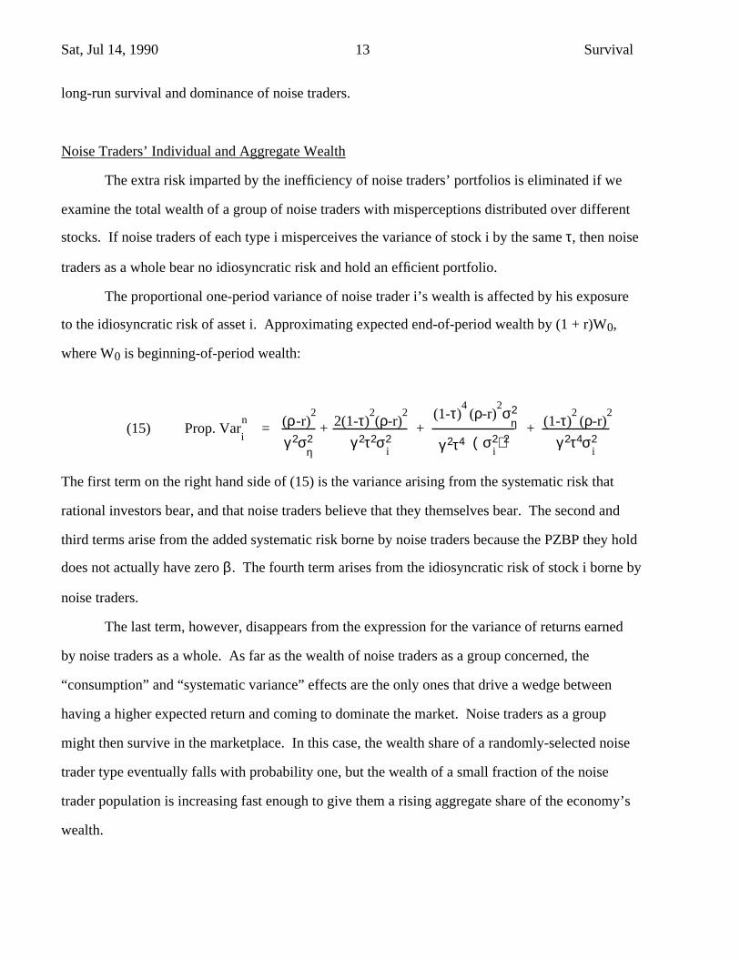
The proportional one-period variance of noise trader i’s wealth is affected by his exposure

to the idiosyncratic risk of asset i. Approximating expected end-of-period wealth by (1 + r)W0,

where W0 is beginning-of-period wealth:

(15) Prop. Vari

n=

γ 2ση2

(ρ-r)2

+ γ 2τ2σ

i2

2(1-τ)2(ρ-r)

2

+ (

(1-τ)4

(ρ-r)2σ

η2

+ γ 2τ4σ

i2

(1-τ)2

(ρ-r)2

σi2)2γ 2τ4

The first term on the right hand side of (15) is the variance arising from the systematic risk that

rational investors bear, and that noise traders believe that they themselves bear. The second and

third terms arise from the added systematic risk borne by noise traders because the PZBP they hold

does not actually have zero β. The fourth term arises from the idiosyncratic risk of stock i borne by

noise traders.

The last term, however, disappears from the expression for the variance of returns earned

by noise traders as a whole. As far as the wealth of noise traders as a group concerned, the

“consumption” and “systematic variance” effects are the only ones that drive a wedge between

having a higher expected return and coming to dominate the market. Noise traders as a group

might then survive in the marketplace. In this case, the wealth share of a randomly-selected noise

trader type eventually falls with probability one, but the wealth of a small fraction of the noise

trader population is increasing fast enough to give them a rising aggregate share of the economy’s

wealth.


Distinguishing Between High Expected Returns and Dominance

For the moment, we neglect consumption and consider only the returns on noise traders’

and rational investors’ portfolios. Assume that investors live forever, face an unchanging distribu-

tion of period-by-period returns, and exhibit constant relative risk aversion. Such investors devote

the same portfolio share to a given asset each period. Their wealth is multiplied by an i.i.d. random

variable (1 + Rt) each period. Taking logs, the random variable ln(1 + Rt) is added to the log of

wealth each period. The law of large numbers tells us that the average expected rate of change, g,

of log wealth is:

(16) g = E(ln(1+Rt)) ≈ ln(1+r) + E(R

t - r) -

2

V(Rt)

taking a second-order Taylor approximation around 1+r, and where V(Rt) is the one period

proportional variance of wealth as in (15).

To evaluate the relative survival chances of noise traders and rational investors, we

therefore consider the difference in their expected rates of change of log wealth, which is

approximately equal to:

(17) E(Rs - R

n) -

2

V

s - V

n

where V is the one period ahead proportional systematic variance of each type’s holdings. The

second “drift” term reflects the likelihood that agents whose returns have a higher variance end up

with lower wealth. Occasional large negative realization of returns decrease such investors’ capital

bases and reduce the future absolute change in their wealth so much that they might eventually

have lower total wealth even if they earn higher period-by-period expected returns. As a result,

investors for whom a larger drift outweighs their advantage of a higher expected return neither

survive nor dominate the market in terms of wealth. If examined after a sufficiently long time

interval, in an overwhelming proportion of cases investors with a higher expected rate of change of

log wealth are richer.

The difference between the expected changes of log wealth for noise traders and rational

investors considered as groups is:


(18)γτ2σi

2

(1-τ) 2(ρ−r)

2{1 - γ

1

- 2γτ

2σi

2

(1-τ) 2σ

η2} .

Because the leading common factor is always positive, the sign of the difference in expected log

wealth changes depends on the terms inside the brackets. The leading 1 inside the brackets reflects

the greater expected returns that noise traders earn because of their unwittingly greater exposure to

systematic risk. The second and third terms capture the increase in aggregate return variance that

this exposure entails.

The third term is small if τ is close to one. In this case as long as investors are more risk

averse than investors with logarithmic utility (have γ>1), considered as a group noise traders who

misperceive variances survive and come to dominate the market. For each γ > 1 there is some δ >

0 such that if |τ-1| < δ then noise traders as a group have a higher expected change in log wealth.

Such noise traders are confused about variances, but their confusion is sufficiently small that the

higher expected return more than outweighs the larger drift induced by the greater variance.

Note, however, that if γ≤1 there is no misperception of the variance of the return distribu-

tion that delivers a higher expected change in log wealth for noise traders. This point is equivalent

to the observation that an investor wishing to maximize the long-run average rate of return earned

on his portfolio should choose portfolio shares as if he had logarithmic utility, i.e. γ=1 (Samuelson,

1971). An investor with γ>1 does not choose such a portfolio because he is sufficiently averse to

low wealth realizations to forego at least some long-run expected return in order to reduce risk.

This implies that all investors who take a position that bears marginally more systematic risk—

even by mistake, as in the case of noise traders—have a higher expected change in log wealth, and

therefore come to dominate rational investors in wealth. Another implication of this is that no type

of noise trader can dominate a rational investor with logarithmic utility.

Conversely, an investor with γ<1 bears too much risk to maximize the long-run average rate

of return on his portfolio. He values the occasional high realization of wealth enough to accept a

substantial chance of having low wealth generated by a risky portfolio. Such an investor could


increase his long-run average rate of return and improve his survival potential by reducing his

holdings of the risky asset. We find the case γ<1 unattractive because investors less risk averse

than log utility fall victim to the St. Petersburg paradox (Samuelson, 1976). Such investors are

willing to pay an infinite amount for a gamble that pays zero with a probability arbitrarily close to

one and pays finite amounts in every state of the world. As we discuss below, γ less than 1 is not

an empirically plausible case.

Consumption

We now turn to the effects of noise traders’ misperceptions on their consumption. If

investors live-- forever, maximize the same approximation to a constant relative risk aversion

utility function as in section III, and face an unchanging distribution of returns, then their

consumption is given by:

(19) ct

= Wt{ γ

γ−1 E(Rt+1

) - 2

γ V(Rt+1

) +

γδ}

where expectations are taken with respect to the perceived distribution of returns (Merton, 1969),

and where δ is the subjective rate of time preference. Since all noise traders consume the same

fraction of wealth, aggregation causes no problems.

Noise traders in this case consume more than do rational investors. They (falsely) believe

that their portfolios have a risk-adjusted net rate of return higher than those of rational investors by:

(20) λi2τ2σi

2 =2γτ

2σi

2

(1−τ) 2(ρ−r)

2

.

Noise traders’ misperceptions lead them to consume a fraction of their wealth higher than that con-

sumed by rational investors by:

(21)W

n

c

n

- W

s

c

s

=2γ 2τ2σ

i2

(γ−1)(1−τ) 2(ρ−r)

2


Conditions for the Long-Run Survival of Noise Traders

Combining (21) with (18) gives an expression for the difference of the expected changes of

noise traders’ and rational investors’ log aggregate wealth. The set of investors with the higher

geometric mean growth rate both survives in the market and comes to dominate in wealth. Noise

traders come to dominate the market in the long run if:

(22)γτ2σi

2

(1-τ)2(ρ−r)2{1 -

γ

1

2γτ2

(1-τ)2(σi2

ση2) -

2γ

γ − 1} > 0 .+

Leaving aside the positive common factor, this expression consists of three pieces. The

leading “1” reflects the higher expected returns earned by noise traders. The final piece arises from

noise traders’ excess consumption. Note that the additional consumption effect is always out-

weighed by the extra return effect. Even though noise traders consume a higher fraction of their

wealth than do rational investors, the average rate of wealth accumulation of noise traders who

misperceive variances alone is always higher than that of rational investors.

The middle two terms of (22) reflect the downward relative drift imposed on the geometric

mean of noise traders’ relative returns by the extra variance of their portfolios. Examination of

(22) reveals that when γ>1 noise traders with small misperceptions survive and come to dominate

the market. We can further simplify (22) to:

(23) (γ − 1) − ( τ

1 − τ)2{σi

2

ση2} > 0 .

By inspection, if γ > 1 (23) holds for τ sufficiently close to one. Moreover, if idiosyncratic risk is

large relative to market risk then (23) holds as long as τ is not too close to zero. Only noise traders

whose misperceptions of returns are truly extraordinary would then fail to dominate the market.

Equations (22) and (23) demonstrate that for all parameters of the return distribution, there are

plausible misperceptions by noise traders that allow them to survive and to dominate the market.


Proposition 2 : For any parameters of the return distribution there exists a δ such that if |τ-1| < δ,

then noise traders who misperceive variances with parameter t survive and come to dominate the

market.

Proof : By inspection of equation (23).

Not only are noise traders who misperceive variances by a small amount and are more risk

averse than log utility guaranteed to survive in the market, but there are many types of noise traders

who misperceive variances by a large amount and yet exhibit a faster degree of wealth

accumulation than rational investors.

A simple calibration exercise demonstrates the empirical plausibility of this result.

Estimates of investors’ degree of relative risk aversion rarely fall below two and are often above

ten. The highest coefficients come from studies that try to reconcile the large risk premia observed

on assets with the relatively smooth growth path of consumption (Mehra and Prescott, 1985; Hall,

1988; and Weil, 1989). Weil in particular finds that representative investor models fit the observed

equity premium only for coefficients of relative risk aversion of 20 or more.2 Similarly, Hall

(1988) finds that the coefficient of relative risk aversion, which in his model is equal to the

intertemporal elasticity of substitution in consumption, is greater than 10. Estimates of relative risk

aversion from individual data are smaller, but they are still greater than one. Friend and Blume

(1975) find using individual household data on portfolio holdings that the degree of relative risk

aversion is greater than two. Gertner (1990) cites a number of studies that generate estimates of

the coefficient of relative risk aversion between 1.5 and 15.

In order to calibrate σi2/ση2, note that market-model regressions of individual security

returns on market returns usually produce R2’s of 0.1 or so, and rarely produce R2’s greater than

0.2 (Roll, 1988). An R2 of .2 corresponds to a σi2/ση2 of 5.

Using these parameter values to calibrate equation (23) reveals that even noise traders who

are grossly overconfident will as a group exhibit higher rates of wealth accumulation. For γ=3 and

σi2/ση2 = 5, equation (23) implies that noise traders who misperceive standard deviations and


have any τ > 0.24—believe that the variance of returns on the assets they favor are not less than 6

% of the true variance—will exhibit higher rates of wealth accumulation. Even for γ=2 and σi/ση

= 1, noise traders will exhibit faster rates of wealth accumulation if they have a τ > 1/2.

We conclude that there is, in fact, a presumption that overconfident investors—even grossly

overconfident investors—will tend to control a higher proportion of the wealth invested in

securities markets as time passes. This presumption is based on the empirical observations that (a)

most investors appear to be more risk averse than log utility, and (b) idiosyncratic risk is large

relative to systematic risk. Under these conditions, investors who are mistaken about the precision

of their estimate of the returns expected from a particular stock will end up taking on more

systematic risk. Taken as a group, these investors will exhibit faster rates of wealth accumulation

than fully rational investors with risk aversion greater than that given by log utility.

V. INVASION

We have interpreted our model as a model of the long run survival and dominance of noise

traders in an environment where they do not affect prices. Our results also apply, with a more

restricted interpretation, to models in which noise traders exert price pressure and distort prices

against themselves. Our conditions sufficient for the dominance of noise traders in a model in

which they do not affect prices have another interpretation in a model where noise traders do affect

prices as conditions sufficient for noise traders to be able to successfully invade the economy, in

the sense that a small group of noise traders introduced into the economy will find that their wealth

share tends to grow, not shrink, over time. Our sufficient conditions can further be interpreted as

conditions sufficient for noise traders to survive in the long run, in the sense of having a share of

the economy’s wealth that is with finite probability bounded away from zero for all time.

When noise traders have an infinitesimal share of wealth, they distort prices and returns

only an infinitesimal amount away from fundamental values. Hence if noise traders have a higher

average rate of wealth accumulation, then they can “invade” even if they distort prices. If their


wealth share is infinitesimal, noise traders will exert negligible price pressure and so their wealth

share will tend to grow. Noise traders therefore survive, in the sense that their wealth share does

not drop toward zero in the long run with probability one. Our analysis of the long run tendency of

the noise trader share in models where they do affect prices is limited to these statements about

“invasion” and “survival.” We can make no statements about the conditions for noise trader domi-

nance in this context, because as soon as they acquire a nontrivial share of wealth they begin to

affect prices in a nontrivial way, and our model and analysis no longer apply.

These results imply that population composed entirely of rational investors is not

“evolutionarily stable” (Maynard Smith, 1982). If a small number of noise traders are introduced

into the population, their relative wealth tends to grow. Noise traders can successfully “invade” the

population. In a world in which investors occasionally “mutated” and changed from noise trader to

rational investor or vice versa, it would be surprising to find a population composed almost entirely

of rational investors.

VI. CONCLUSION

We have presented a model of portfolio allocation by noise traders who form incorrect

expectations chiefly about the variance of the return distribution of a particular asset. We showed

that for plausible misperceptions, such noise traders as a group can not only earn higher returns

than do rational investors but also survive and dominate the market in terms of wealth in the long

run. Such long run success of noise traders occurs despite their excessive risk taking and excessive

consumption. The case against their long run viability is by no means as clearcut as is commonly

supposed.

The main limitation of our model is that it does not allow noise traders to affect prices.

This paper therefore cannot address Friedman’s main point: that noise traders buy high and sell

low. In our earlier paper (De Long, Shleifer, Summers, and Waldmann, 1990) we have shown that

noise traders can earn higher expected returns than rational investors even when they buy high and

sell low. But the model of our earlier paper could not deal with survival and dominance because


the wealth of investors was held fixed. The next step in this literature, then, is to arrive at a

tractable model in which noise traders affect prices and in which survival and dominance can be

analyzed. The answers afforded by such a model would go a long way toward settling the question

raised by Friedman (1953).


REFERENCES

Alpert, M. and Raiffa, H. 1959. A Progress Report on the Training of Probability Assessors.Reprinted in Kahneman, D.; Slovic, P.; and Tversky, A. (eds.) 1982. Judgment Under Uncertainty: Heuristics and Biases. Cambridge, U.K.: Cambridge University Press.

Andreassen, P., and Kraus, S. 1987. Intuitive Prediction by Extrapolation: The Stock Market,Exponential Growth, Divorce, and the Salience of Change. Harvard University mimeo.

Black, F. 1986. Noise. Journal of Finance Proceedings 41 (July): 529-43.

Campbell, J.Y., and Kyle, A.S. 1986. Smart Money, Noise Trading, and Stock Price Behavior.Princeton University mimeo.

De Long, J. B.; Shleifer,A.M.; Summers, L.H.; and Waldmann, R.J. 1990. Noise Trader Risk inFinancial Markets. Journal of Political Economy 98 (August): 703–38.

Einhorn , H., and Hogarth, R. 1978. Confidence in Judgment: Persistence of the Illusion ofValidity Psychological Review 85 (September): 395-416.

Figlewski, S. 1979. Market ‘Efficiency’ in a Market with Heterogeneous Information. Journal of Political Economy 86 (August): 581-97.

Friedman, M. 1953. The Case for Flexible Exchange Rates. In Essays in Positive Economics. Chicago: University of Chicago Press.

Friend, I., and Blume, M. 1975. The Demand for Risky Assets. American Economic Review 65(December): 900-922.

Gertner, R. 1990. Game Shows and Economic Behavior: Risk Taking on Card Sharks. Universityof Chicago Business School mimeo.

Gilovich, T.; Valone, R.; and Tversky, A. 1985. The Hot Hand in Basketball: On theMisperception of Random Sequences. Cognitive Psychology 17 (July): 295-314.

Hall, R. 1988. Intertemporal Substitution in Consumption. Journal of Political Economy 96(April): 339–57.

Kahneman, D., and Tversky, A. 1973. On the Psychology of Prediction. Psychological Review 80(July): 237-51.

Kahneman, D.; Slovic, P.; and Tversky, A. (eds.) 1982. Judgment Under Uncertainty: Heuristics and Biases . Cambridge, UK: Cambridge University Press.

Kyle, A.S. 1985. Continuous Auctions and Insider Trading. Econometrica 53 (November): 1315-36.

Langer, E.J. (1975). The Illusion of Control. Journal of Personality and Social Psychology 32(August): 311-28.

Lease, R.C.; Lewellen, W.G.; and Schlarbaum, G.G. 1974. The Individual Investor: Attributes andAttitudes. Journal of Finance 29 (May): 413-33.

Lichtenstein, S.; Fischhoff, B.; and Phillips, L. 1982. Calibration of Probabilities: The State of the


Art as of 1980. In Kahneman, D.; Slovic, P.; and Tversky, A. (eds.) 1982. Judgment Under Uncertainty: Heuristics and Biases. Cambridge, UK: Cambridge University Press.

Maynard Smith, J. 1982. Evolution and the Theory of Games. Cambridge, UK: CambridgeUniversity Press.

Mehra, R., and Prescott, E. 1985. The Equity Premium: A Puzzle. Journal of Monetary Economics 15 (March): 145–61.

Merton, R. 1969. Optimal Portfolio Selection by Dynamic Stochastic Programming. Review of Economics and Statistics 51 (August): 247–57.

Pagano, M. 1989. Trading Volume and Asset Liquidity. Quarterly Journal of Economics 104(May): 255–74.

Roll, R. 1988. R2. Journal of Finance Proceedings 43 (July): 541–66.

Samuelson, P.A. 1971. The ‘Fallacy’ of Maximizing the Geometric Mean in Long Sequences ofInvesting or Gambling. Proceedings of the National Academy of Sciences 68 (October):2493-6.

Samuelson, P.A. 1977. St. Petersburg Paradoxes. Journal of Economic Literature 15 (March): 24–55.

Shiller, R. 1984. Stock Prices and Social Dynamics. Brookings Papers on Economic Activity (Fall): 457-98.

Slovic, P. 1982. Toward Understanding and Improving Decisions. In Howell, W. (ed.) Human Performance and Productivity . Hillsdale, NJ: Erlbaum Press.

Stein, J. 1987. Informational Externalities and Welfare-Reducing Speculation. Journal of Political Economy 95 (December): 1123-45.

Tversky, A., and Kahneman, D. 1971. The Belief in the ‘Law of Small Numbers’. Psychological Bulletin 76 (August): 105-10.

Tversky, A., and Kahneman, D. 1974. Judgment Under Uncertainty: Heuristics and Biases. Science 185 (September 27): 1124-31.

Weil, P. 1989. The Equity Premium Puzzle and the Risk-Free Rate Puzzle. Journal of Monetary Economics 24 (November): 401-21.


Rational investorsearn higher returns

overestimation of mean return

correct perception of mean return

underestimation of mean return

µ = 1

τ = 1 overestimation ofstandard deviationcorrect perception of

standard deviation

underestimation ofstandard deviation

45˚

µ = τ

Noise traders earnhigher returns


FIGURE 1

AREA OF ( ) SPACE WHERE NOISE TRADERS EARN HIGHER RETURNS

THAN RATIONAL INVESTORS


NOTES

*We would like to thank the Alfred P. Sloan and Russell Sage Foundations for financial support.

We are also grateful to David Cutler, James Poterba, and especially the referee from the Journal of

Business for helpful comments.

1Pagano (1987) studies thin markets where, even though noise traders’ misperceptions are

uncorrelated, their trades need not cancel out. We assume that markets are thick enough that the

law of large numbers applies.

2Although, as he points out, such models are then unable to fit the relatively low realized safe real

rate of return.

Documents

THE SURVIVAL OF NOISE TRADERS IN FINANCIAL … SURVIVAL OF NOISE TRADERS IN FINANCIAL MARKETS * J. Bradford De Long, Andrei Shleifer, Lawrence H. Summers, and Robert J. Waldmann Harvard