Embed Size (px)
Citation preview
The t Distribution and its Applications
James H. Steiger
Department of Psychology and Human DevelopmentVanderbilt University
James H. Steiger (Vanderbilt University) 1 / 51
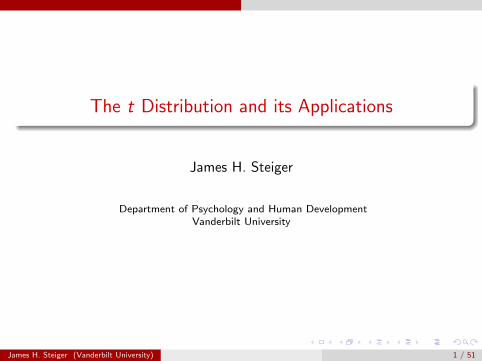
The t Distribution and its Applications1 Introduction
2 Student’s t Distribution
Basic Facts about Student’s t
3 Relationship to the One-Sample t
Distribution of the Test Statistic
The General Approach to Power Calculation
Power Calculation for the 1-Sample t
Sample Size Calculation for the 1-Sample t
4 Relationship to the t Test for Two Independent Samples
Distribution of the Test Statistic
Power Calculation for the 2-Sample t
Sample Size Calculation for the 2-Sample t
5 Relationship to the Correlated Sample t
Distribution of the Correlated Sample t Statistic
6 Distribution of the Generalized t Statistic
Sample Size Estimation in the Generalized t
7 Power Analysis via Simulation
James H. Steiger (Vanderbilt University) 2 / 51
Introduction
Introduction
In this module, we review some properties of Student’s t distribution.
We shall then relate these properties to the null and non-nulldistribution of three classic test statistics:
1 The 1-Sample Student’s t-test for a single mean.
2 The 2-Sample independent sample t-test for comparing two means.
3 The 2-Sample “correlated sample” t-test for comparing two meanswith correlated or repeated-measures data.
We then discuss power and sample size calculations using thedeveloped facts.
James H. Steiger (Vanderbilt University) 3 / 51
Student’s t Distribution
Student’s t Distribution
In a preceding module, we discussed the classic z-statistic for testinga single mean when the population variance is somehow known.
Student’s t-distribution was developed in response to the reality that,unfortunately, σ2 is not known in the vast majority of situations.
Although substitution of a consistent sample-based estimate of σ2
(such as s2, the familiar sample variance) will yield a statistic that isstill asymptotically normal, the statistic will no longer have an exactnormal distribution even when the population distribution is normal.
The question of precisely what the distribution of
Y • − µ0√s2/n
(1)
is when the observations are i.i.d. normal was answered by “Student.”
James H. Steiger (Vanderbilt University) 4 / 51
Student’s t Distribution Basic Facts about Student’s t
Student’s t Distribution
The pdf and cdf of the t-distribution are readily available online atplaces like Wikipedia and Mathworld.
The formulae for the functions need not concern us here — they arebuilt into R.
The key facts, for our purposes, are summarized on the following slide.
James H. Steiger (Vanderbilt University) 5 / 51
Student’s t Distribution Basic Facts about Student’s t
Student’s t Distribution
The t distribution, in its more general form, has two parameters:
1 The degrees of freedom, ν
2 The noncentrality parameter, δ
When δ = 0, the distribution is said to be the “central Student’s t,”or simply the “t distribution.”
When δ 6= 0, the distribution is said to be the “noncentral Student’st,” or simply the “noncentral t distribution.”
The central t distribution has a mean of 0 and a variance slightlylarger than the standard normal distribution. The kurtosis is alsoslightly larger than 3.
The central t distribution is symmetric, while the noncentral t isskewed in the direction of δ.
James H. Steiger (Vanderbilt University) 6 / 51
Student’s t Distribution Basic Facts about Student’s t
Student’s t DistributionDistributional Characterization
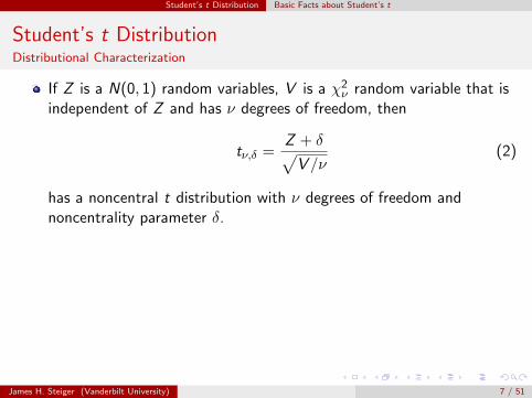
If Z is a N(0, 1) random variables, V is a χ2ν random variable that is
independent of Z and has ν degrees of freedom, then
tν,δ =Z + δ√
V /ν(2)
has a noncentral t distribution with ν degrees of freedom andnoncentrality parameter δ.
James H. Steiger (Vanderbilt University) 7 / 51
Relationship to the One-Sample t Distribution of the Test Statistic
Distribution of the 1-Sample t
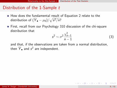
How does the fundamental result of Equation 2 relate to thedistribution of (Y • − µ0)/
√s2/n?
First, recall from our Psychology 310 discussion of the chi-squaredistribution that
s2 ∼ σ2 χ2n−1
n − 1(3)
and that, if the observations are taken from a normal distribution,then Y • and s2 are independent.
James H. Steiger (Vanderbilt University) 8 / 51
Relationship to the One-Sample t Distribution of the Test Statistic
Distribution of the 1-Sample t
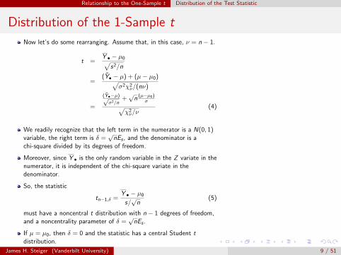
Now let’s do some rearranging. Assume that, in this case, ν = n − 1.
t =Y • − µ0√
s2/n
=(Y• − µ) + (µ− µ0)√
σ2χ2ν/(nν)
=
(Y•−µ)√σ2/n
+√
n (µ−µ0)σ√
χ2ν/ν
(4)
We readily recognize that the left term in the numerator is a N(0, 1)variable, the right term is δ =
√nEs , and the denominator is a
chi-square divided by its degrees of freedom.
Moreover, since Y • is the only random variable in the Z variate in thenumerator, it is independent of the chi-square variate in thedenominator.
So, the statistic
tn−1,δ =Y • − µ0
s/√
n(5)
must have a noncentral t distribution with n − 1 degrees of freedom,and a noncentrality parameter of δ =
√nEs .
If µ = µ0, then δ = 0 and the statistic has a central Student tdistribution.
James H. Steiger (Vanderbilt University) 9 / 51
Relationship to the One-Sample t The General Approach to Power Calculation
The General Approach to Power Calculation
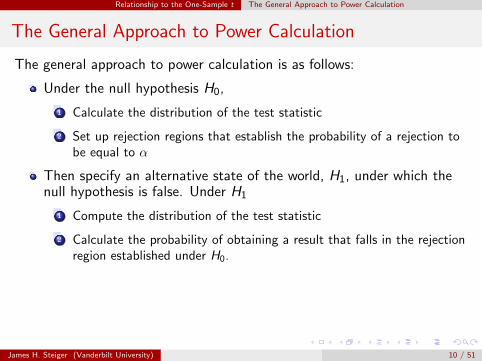
The general approach to power calculation is as follows:
Under the null hypothesis H0,
1 Calculate the distribution of the test statistic
2 Set up rejection regions that establish the probability of a rejection tobe equal to α
Then specify an alternative state of the world, H1, under which thenull hypothesis is false. Under H1
1 Compute the distribution of the test statistic
2 Calculate the probability of obtaining a result that falls in the rejectionregion established under H0.
James H. Steiger (Vanderbilt University) 10 / 51
Relationship to the One-Sample t The General Approach to Power Calculation
The General Approach to Power Calculation
Note the following key points:
Developing expressions for the exact null and non-null distributions ofthe test statistic often requires some specialized statistical knowledge.
In general, it is much more likely that expressions for the nulldistribution of the test statistic will be available than expressions forthe non-null distribution.
Fortunately, statistical simulation will often provide a reasonablealternative to exact calculation.
James H. Steiger (Vanderbilt University) 11 / 51
Relationship to the One-Sample t Power Calculation for the 1-Sample t
Power Calculation for the 1-Sample t
Power calculation for the 1-Sample t is straightforward if we followthe usual steps.
Suppose, as with the z-test example, we are pursuing a 1-Samplehypothesis test that specifies H0 : µ ≤ 70 against the alternative thatH1 : µ > 70. We will be using a sample of n = 25 observations, withα = 0.05.
If the null hypothesis is true, the test statistic will have a central tdistribution with n − 1 = 24 degrees of freedom.
The (one-tailed) critical value will be
> qt(0.95, 24)
[1] 1.710882
What will the power of the test be if µ = 75 and σ = 10?
James H. Steiger (Vanderbilt University) 12 / 51
Relationship to the One-Sample t Power Calculation for the 1-Sample t
Power Calculation for the 1-Sample t
In this case, the non-null distribution is noncentral t, with 24 degreesof freedom, and a noncentrality parameter of√
nEs =√
25(75− 70)/10 = 2.5.
So power is the probability of exceeding the rejection point in thisnoncentral t distribution.
> 1 - pt(qt(0.95, 24), 24, 2.5)
[1] 0.7833861
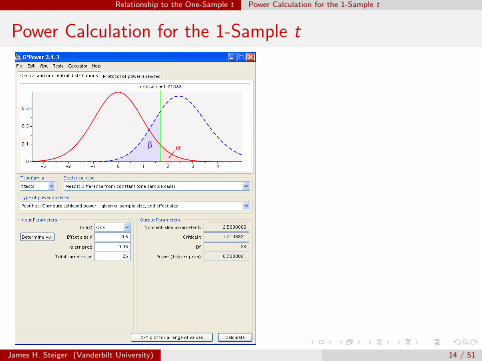
Gpower gets the identical result, as shown on the next slide.
James H. Steiger (Vanderbilt University) 13 / 51
Relationship to the One-Sample t Power Calculation for the 1-Sample t
Power Calculation for the 1-Sample t
James H. Steiger (Vanderbilt University) 14 / 51
Relationship to the One-Sample t Power Calculation for the 1-Sample t
Power Calculation for the 1-Sample t
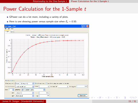
GPower can do a lot more, including a variety of plots.
Here is one showing power versus sample size when Es = 0.50.
James H. Steiger (Vanderbilt University) 15 / 51
Relationship to the One-Sample t Power Calculation for the 1-Sample t
Power Calculation for the 1-Sample t
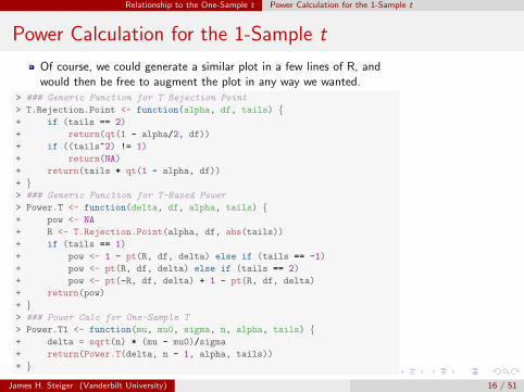
Of course, we could generate a similar plot in a few lines of R, andwould then be free to augment the plot in any way we wanted.
> ### Generic Function for T Rejection Point
> T.Rejection.Point <- function(alpha, df, tails) {+ if (tails == 2)
+ return(qt(1 - alpha/2, df))
+ if ((tails^2) != 1)
+ return(NA)
+ return(tails * qt(1 - alpha, df))
+ }> ### Generic Function for T-Based Power
> Power.T <- function(delta, df, alpha, tails) {+ pow <- NA
+ R <- T.Rejection.Point(alpha, df, abs(tails))
+ if (tails == 1)
+ pow <- 1 - pt(R, df, delta) else if (tails == -1)
+ pow <- pt(R, df, delta) else if (tails == 2)
+ pow <- pt(-R, df, delta) + 1 - pt(R, df, delta)
+ return(pow)
+ }> ### Power Calc for One-Sample T
> Power.T1 <- function(mu, mu0, sigma, n, alpha, tails) {+ delta = sqrt(n) * (mu - mu0)/sigma
+ return(Power.T(delta, n - 1, alpha, tails))
+ }
James H. Steiger (Vanderbilt University) 16 / 51
Relationship to the One-Sample t Power Calculation for the 1-Sample t
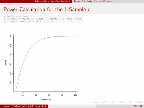
Power Calculation for the 1-Sample t> ### Plot Power Curve
> curve(Power.T1(75, 70, 10, x, 0.05, 1), 10, 100, xlab = "Sample Size",
+ ylab = "Power", col = "red")
20 40 60 80 100
0.5
0.6
0.7
0.8
0.9
1.0
Sample Size
Pow
er
James H. Steiger (Vanderbilt University) 17 / 51
Relationship to the One-Sample t Sample Size Calculation for the 1-Sample t
Sample Size Calculation for the 1-Sample t
In the 1-sample z test for a single mean, we saw in Psychology 310that it is possible to develop an equation that directly calculates thesample size required to yield a desired level of power.
However, in most cases, a closed-form solution for n is not available,because the shape of the test statistic changes along with its locationand spread as a function of n and the effect size.
Consequently, in most cases iterative methods must be employed.These methods try an initial value for n, compute an “improvementdirection”, and step the value of n in that direction, until thedifference between the computed power and desired power dropsbelow a target value.
With modern software, the target n is found in less than a second formost problems.
James H. Steiger (Vanderbilt University) 18 / 51
Relationship to the One-Sample t Sample Size Calculation for the 1-Sample t
Sample Size Calculation for the 1-Sample t
Modern power calculation software handles many of the classic casesin parametric statistics. However, in more complex circumstances,remember that, through the use of R’s extensive simulation andplotting capabilities, you can obtain power curves and sample-sizecalculations in situations that “canned” software cannot handle.
The approach is simple. Plot power versus sample size, then home inon a narrow region of the plot to determine just where sample sizebecomes barely large enough to yield desired power.
James H. Steiger (Vanderbilt University) 19 / 51
Relationship to the One-Sample t Sample Size Calculation for the 1-Sample t
Sample Size Calculation for the 1-Sample tAn Example
Example (Sample Size Calculation)
Let’s try calculating the required sample size to achieve a power of0.95 when Es = 0.80, and the test is two-sided with α = 0.01. We’lluse the graphical approach. Here is a preliminary plot. Notice againthat Es can be input directly by setting µ0 = 0 and σ = 1 and settingµ = Es .In a couple of seconds, we have the required n narrowed down tobetween 30 and 35.
James H. Steiger (Vanderbilt University) 20 / 51
Relationship to the One-Sample t Sample Size Calculation for the 1-Sample t
Sample Size Calculation for the 1-Sample tAn Example
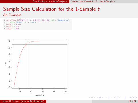
> curve(Power.T1(0.8, 0, 1, x, 0.01, 2), 10, 100, xlab = "Sample Size",
+ ylab = "Power", col = "red")
> abline(h = 0.95)
> abline(v = 30)
> abline(v = 35)
20 40 60 80 100
0.3
0.4
0.5
0.6
0.7
0.8
0.9
1.0
Sample Size
Pow
er
James H. Steiger (Vanderbilt University) 21 / 51
Relationship to the One-Sample t Sample Size Calculation for the 1-Sample t
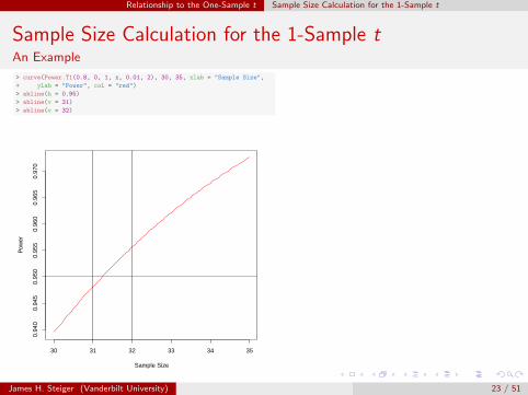
Sample Size Calculation for the 1-Sample tAn Example
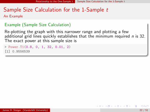
Example (Sample Size Calculation)
Re-plotting the graph with this narrower range and plotting a fewadditional grid lines quickly establishes that the minimum required n is 32.The exact power at this sample size is
> Power.T1(0.8, 0, 1, 32, 0.01, 2)
[1] 0.9556539
James H. Steiger (Vanderbilt University) 22 / 51
Relationship to the One-Sample t Sample Size Calculation for the 1-Sample t
Sample Size Calculation for the 1-Sample tAn Example
> curve(Power.T1(0.8, 0, 1, x, 0.01, 2), 30, 35, xlab = "Sample Size",
+ ylab = "Power", col = "red")
> abline(h = 0.95)
> abline(v = 31)
> abline(v = 32)
30 31 32 33 34 35
0.94
00.
945
0.95
00.
955
0.96
00.
965
0.97
0
Sample Size
Pow
er
James H. Steiger (Vanderbilt University) 23 / 51
Relationship to the One-Sample t Sample Size Calculation for the 1-Sample t
Sample Size Calculation for the 1-Sample tAn Example
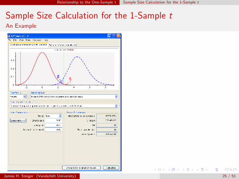
Example (Sample Size Calculation)
GPower automates the process, and yields the identical answer, as shownbelow.
James H. Steiger (Vanderbilt University) 24 / 51
Relationship to the One-Sample t Sample Size Calculation for the 1-Sample t
Sample Size Calculation for the 1-Sample tAn Example
James H. Steiger (Vanderbilt University) 25 / 51
Relationship to the t Test for Two Independent Samples Distribution of the Test Statistic
Distribution of the 2-Sample t
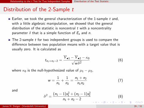
Earlier, we took the general characterization of the 1-sample t and,with a little algebraic manipulation, we showed that the generaldistribution of the statistic is noncentral t with a noncentralityparameter δ that is a simple function of Es and n.
The 2-sample t for two independent groups is used to compare thedifference between two population means with a target value that isusually zero. It is calculated as
tn1+n2−2 =Y •1 − Y •2 − κ0√
w σ2(6)
where κ0 is the null-hypothesized value of µ1 − µ2,
w =1
n1+
1
n2=
n1 + n2
n1n2(7)
and
σ2 =(n1 − 1)s2
1 + (n2 − 1)s22
n1 + n2 − 2(8)
James H. Steiger (Vanderbilt University) 26 / 51
Relationship to the t Test for Two Independent Samples Distribution of the Test Statistic
Distribution of the 2-Sample t
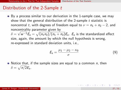
By a process similar to our derivation in the 1-sample case, we mayshow that the general distribution of the 2-sample t statistic isnoncentral t, with degrees of freedom equal to ν = n1 + n2 − 2, andnoncentrality parameter given byδ =√
w−1Es =√
(n1n2)/(n1 + n2)Es . Es is the standardized effectsize, again, the amount by which the null hypothesis is wrong,re-expressed in standard deviation units, i.e.,
Es =µ1 − µ2 − κ0
σ(9)
Notice that, if the sample sizes are equal to a common n, thenδ =
√n/2Es .
James H. Steiger (Vanderbilt University) 27 / 51
Relationship to the t Test for Two Independent Samples Power Calculation for the 2-Sample t
Power Calculation for the 2-Sample t
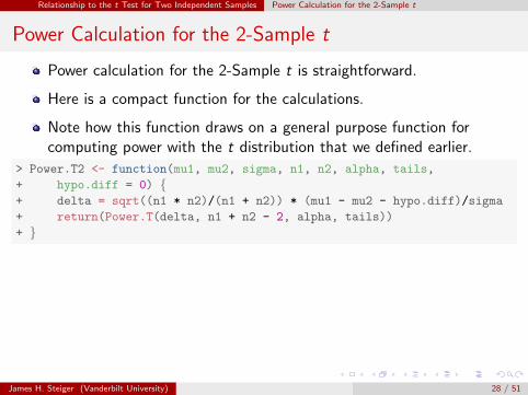
Power calculation for the 2-Sample t is straightforward.
Here is a compact function for the calculations.
Note how this function draws on a general purpose function forcomputing power with the t distribution that we defined earlier.
> Power.T2 <- function(mu1, mu2, sigma, n1, n2, alpha, tails,
+ hypo.diff = 0) {+ delta = sqrt((n1 * n2)/(n1 + n2)) * (mu1 - mu2 - hypo.diff)/sigma
+ return(Power.T(delta, n1 + n2 - 2, alpha, tails))
+ }
James H. Steiger (Vanderbilt University) 28 / 51

Relationship to the t Test for Two Independent Samples Power Calculation for the 2-Sample t
Power Calculation for the 2-Sample t
Suppose we wish to calculate the power to detect Es = 0.50, whenn1 = n2 = 20, α = .05, and the test is 2-sided.
Again, note how we “trick” the power analysis function by enteringµ2 = 0, σ = 1, and replacing µ2 with Es .
> Power.T2(0.5, 0, 1, 20, 20, 0.05, 2)
[1] 0.337939
James H. Steiger (Vanderbilt University) 29 / 51
Relationship to the t Test for Two Independent Samples Sample Size Calculation for the 2-Sample t
Sample Size Calculation for the 2-Sample t
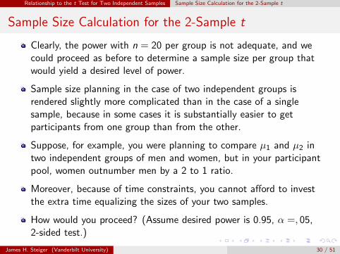
Clearly, the power with n = 20 per group is not adequate, and wecould proceed as before to determine a sample size per group thatwould yield a desired level of power.
Sample size planning in the case of two independent groups isrendered slightly more complicated than in the case of a singlesample, because in some cases it is substantially easier to getparticipants from one group than from the other.
Suppose, for example, you were planning to compare µ1 and µ2 intwo independent groups of men and women, but in your participantpool, women outnumber men by a 2 to 1 ratio.
Moreover, because of time constraints, you cannot afford to investthe extra time equalizing the sizes of your two samples.
How would you proceed? (Assume desired power is 0.95, α =, 05,2-sided test.)
James H. Steiger (Vanderbilt University) 30 / 51
Relationship to the t Test for Two Independent Samples Sample Size Calculation for the 2-Sample t
Sample Size Calculation for the 2-Sample tUnequal Group Proportions
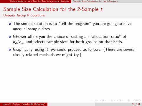
The simple solution is to “tell the program” you are going to haveunequal sample sizes.
GPower offers you the choice of setting an “allocation ratio” ofn2/n1, and selects sample sizes for both groups on that basis.
Graphically, using R, we could proceed as follows. (There are severalclosely related methods we might try.)
James H. Steiger (Vanderbilt University) 31 / 51
Relationship to the t Test for Two Independent Samples Sample Size Calculation for the 2-Sample t
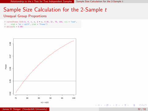
Sample Size Calculation for the 2-Sample tUnequal Group Proportions
> curve(Power.T2(0.5, 0, 1, x, 2 * x, 0.05, 2), 75, 100, col = "red",
+ xlab = "n1 = n2/2", ylab = "Power")
> abline(h = 0.95)
75 80 85 90 95 100
0.94
0.95
0.96
0.97
0.98
n1 = n2/2
Pow
er
James H. Steiger (Vanderbilt University) 32 / 51
Relationship to the t Test for Two Independent Samples Sample Size Calculation for the 2-Sample t
Sample Size Calculation for the 2-Sample tUnequal Group Proportions
In a few seconds, we can determine that n1 = 79 and n2 = 158 willproduce power slightly exceeding 0.95.
In fact, we still would have power slightly exceeding 0.95 if wedropped n2 to 157.
However, given the guesswork involved and the probability of at leastminor assumption violations, such hairsplitting seems unnecessaryand, indeed, somewhat pedantic.
James H. Steiger (Vanderbilt University) 33 / 51
Relationship to the Correlated Sample t Distribution of the Correlated Sample t Statistic
Distribution of the Correlated Sample t Statistic
In the correlated sample t statistic, n observations are observed fortwo groups.
These observations represent either matched (or correlated) samples,or repeated measures on the same individuals.
The correlated sample t statistic is actually a 1-sample t calculatedon the difference scores.
The null hypothesis compares the mean of the difference scores with ahypothesized mean difference κ0, which usually is set equal to zero.
Consequently, the distribution of the correlated sample t is noncentralt, with n − 1 degrees of freedom, and a noncentrality parameter of
δ =√
nE ∗s =√
nµ1 − µ2 − κ0
σdiff(10)
James H. Steiger (Vanderbilt University) 34 / 51
Relationship to the Correlated Sample t Distribution of the Correlated Sample t Statistic
Distribution of the Correlated Sample t StatisticA Caveat
Clearly, we can process the power and sample size calculations for thecorrelated sample t with essentially the same mechanics as we usedfor the 1-sample t. You will note that the GPower input dialog for thecorrelated sample test looks virtually identical to the input dialog forthe 1-sample test.
However, it is important to realize that, in a conceptual sense, the“standardized effect size” we input in the 2-sample correlated sampletest is not the same as in the 2-sample independent sample case.This is why I marked it with an asterisk.
James H. Steiger (Vanderbilt University) 35 / 51
Relationship to the Correlated Sample t Distribution of the Correlated Sample t Statistic
Distribution of the Correlated Sample t StatisticA Caveat
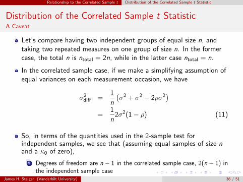
Let’s compare having two independent groups of equal size n, andtaking two repeated measures on one group of size n. In the formercase, the total n is ntotal = 2n, while in the latter case ntotal = n.
In the correlated sample case, if we make a simplifying assumption ofequal variances on each measurement occasion, we have
σ2diff =
1
n
(σ2 + σ2 − 2ρσ2
)=
1
n2σ2(1− ρ) (11)
So, in terms of the quantities used in the 2-sample test forindependent samples, we see that (assuming equal samples of size nand a κ0 of zero),
1 Degrees of freedom are n− 1 in the correlated sample case, 2(n− 1) inthe independent sample case
James H. Steiger (Vanderbilt University) 36 / 51
Relationship to the Correlated Sample t Distribution of the Correlated Sample t Statistic
Distribution of the Correlated Sample t StatisticA Caveat
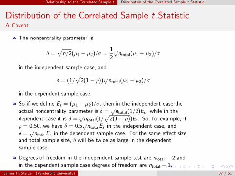
The noncentrality parameter is
δ =√
n/2(µ1 − µ2)/σ =1
2
√ntotal(µ1 − µ2)/σ
in the independent sample case, and
δ = (1/√
2(1− ρ))√
ntotal(µ1 − µ2)/σ
in the dependent sample case.
So if we define Es = (µ1 − µ2)/σ, then in the independent case theactual noncentrality parameter is δ =
√ntotal(1/2)Es , while in the
dependent case it is δ =√
ntotal(1/√
2(1− ρ))Es . So, for example, ifρ = 0.50, we have δ = 0.5
√ntotalEs in the independent case, and
δ =√
ntotalEs in the dependent sample case. For the same effect sizeand total sample size, δ will be twice as large in the dependentsample case.
Degrees of freedom in the independent sample test are ntotal − 2 andin the dependent sample case degrees of freedom are ntotal − 1.
James H. Steiger (Vanderbilt University) 37 / 51
Relationship to the Correlated Sample t Distribution of the Correlated Sample t Statistic
Distribution of the Correlated Sample t StatisticA Caveat
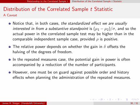
Notice that, in both cases, the standardized effect we are usuallyinterested in from a substantive standpoint is (µ1 − µ2)/σ, and so theactual power in the correlated sample test may be higher than in thecomparable independent sample case, provided ρ is positive.
The relative power depends on whether the gain in δ offsets thehalving of the degrees of freedom.
In the repeated measures case, the potential gain in power is oftenaccompanied by a reduction of the number of participants.
However, one must be on guard against possible order and historyeffects when planning the administration of the repeated measures.
James H. Steiger (Vanderbilt University) 38 / 51
Relationship to the Correlated Sample t Distribution of the Correlated Sample t Statistic
Distribution of the Correlated Sample t StatisticA Caveat
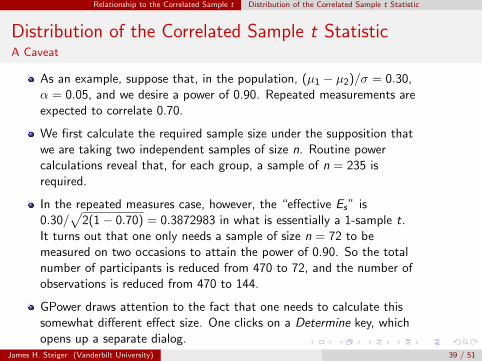
As an example, suppose that, in the population, (µ1 − µ2)/σ = 0.30,α = 0.05, and we desire a power of 0.90. Repeated measurements areexpected to correlate 0.70.
We first calculate the required sample size under the supposition thatwe are taking two independent samples of size n. Routine powercalculations reveal that, for each group, a sample of n = 235 isrequired.
In the repeated measures case, however, the “effective Es” is0.30/
√2(1− 0.70) = 0.3872983 in what is essentially a 1-sample t.
It turns out that one only needs a sample of size n = 72 to bemeasured on two occasions to attain the power of 0.90. So the totalnumber of participants is reduced from 470 to 72, and the number ofobservations is reduced from 470 to 144.
GPower draws attention to the fact that one needs to calculate thissomewhat different effect size. One clicks on a Determine key, whichopens up a separate dialog.
James H. Steiger (Vanderbilt University) 39 / 51
Relationship to the Correlated Sample t Distribution of the Correlated Sample t Statistic
Distribution of the Correlated Sample t StatisticAssumptions
The assumptions for the correlated sample t test are a bit differentfrom those of the 2-sample independent sample test.
The correlated sample test requires the assumption of bivariatenormality, which is a stronger condition than having data in eachcondition be normally distributed.
The correlated sample test, on the other hand, does not require theassumption of equal variances, because the two sets of observationsare collapsed into one prior to the final calculations.
James H. Steiger (Vanderbilt University) 40 / 51
Relationship to the Correlated Sample t Distribution of the Correlated Sample t Statistic
Power Calculation in the Correlated Sample tAssumptions
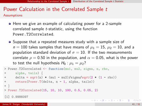
Here we give an example of calculating power for a 2-samplecorrelated sample t-statistic, using the functionPower.T2Correlated.
Suppose that a repeated measures study with a sample size ofn = 100 takes samples that have means of µ1 = 15, µ2 = 10, and apopulation standard deviation of σ = 10. If the two measurementscorrelate ρ = 0.50 in the population, and α = 0.05, what is the powerto test the null hypothesis H0 : µ1 = µ2?
> Power.T2Correlated <- function(mu1, mu2, sigma, n, rho,
+ alpha, tails) {+ delta = sqrt(n) * (mu1 - mu2)/sigma/sqrt(2 * (1 - rho))
+ return(Power.T(delta, n - 1, alpha, tails))
+ }> Power.T2Correlated(15, 10, 10, 100, 0.5, 0.05, 2)
[1] 0.9986097
James H. Steiger (Vanderbilt University) 41 / 51
Distribution of the Generalized t Statistic
Distribution of the Generalized t Statistic
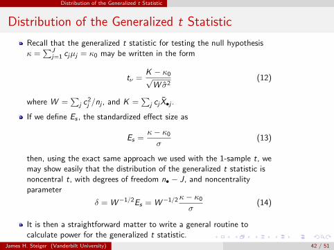
Recall that the generalized t statistic for testing the null hypothesisκ =
∑Jj=1 cjµj = κ0 may be written in the form
tν =K − κ0√
W σ2(12)
where W =∑
j c2j /nj , and K =
∑j cj X•j .
If we define Es , the standardized effect size as
Es =κ− κ0
σ(13)
then, using the exact same approach we used with the 1-sample t, wemay show easily that the distribution of the generalized t statistic isnoncentral t, with degrees of freedom n• − J, and noncentralityparameter
δ = W −1/2Es = W −1/2κ− κ0
σ(14)
It is then a straightforward matter to write a general routine tocalculate power for the generalized t statistic.
James H. Steiger (Vanderbilt University) 42 / 51
Distribution of the Generalized t Statistic
Power Calculation for the Generalized t
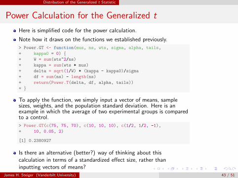
Here is simplified code for the power calculation.
Note how it draws on the functions we established previously.
> Power.GT <- function(mus, ns, wts, sigma, alpha, tails,
+ kappa0 = 0) {+ W = sum(wts^2/ns)
+ kappa = sum(wts * mus)
+ delta = sqrt(1/W) * (kappa - kappa0)/sigma
+ df = sum(ns) - length(ns)
+ return(Power.T(delta, df, alpha, tails))
+ }
To apply the function, we simply input a vector of means, samplesizes, weights, and the population standard deviation. Here is anexample in which the average of two experimental groups is comparedto a control.
> Power.GT(c(75, 75, 70), c(10, 10, 10), c(1/2, 1/2, -1),
+ 10, 0.05, 2)
[1] 0.2380927
Is there an alternative (better?) way of thinking about thiscalculation in terms of a standardized effect size, rather thaninputting vectors of means?
James H. Steiger (Vanderbilt University) 43 / 51
Distribution of the Generalized t Statistic Sample Size Estimation in the Generalized t
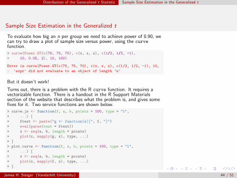
Sample Size Estimation in the Generalized t
To evaluate how big an n per group we need to achieve power of 0.90, wecan try to draw a plot of sample size versus power, using the curvefunction.
> curve(Power.GT(c(75, 75, 70), c(x, x, x), c(1/2, 1/2, -1),
+ 10, 0.05, 2), 10, 100)
Error in curve(Power.GT(c(75, 75, 70), c(x, x, x), c(1/2, 1/2, -1), 10,
: ’expr’ did not evaluate to an object of length ’n’
But it doesn’t work!
Turns out, there is a problem with the R curve function. It requires avectorizable function. There is a handout in the R Support Materialssection of the website that describes what the problem is, and gives somefixes for it. Two service functions are shown below.
> curve.js <- function(f, a, b, points = 100, type = "l",
+ ...) {+ ftext <- paste("g <- function(x){", f, "}")+ eval(parse(text = ftext))
+ x <- seq(a, b, length = points)
+ plot(x, mapply(g, x), type, ...)
+ }> plot.curve <- function(f, a, b, points = 100, type = "l",
+ ...) {+ x <- seq(a, b, length = points)
+ plot(x, mapply(f, x), type, ...)
+ }
James H. Steiger (Vanderbilt University) 44 / 51
Distribution of the Generalized t Statistic Sample Size Estimation in the Generalized t
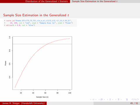
Sample Size Estimation in the Generalized t
> curve.js("Power.GT(c(75,75,70),c(x,x,x),c(1/2,1/2,-1),10,0.05,2)",
+ 10, 100, col = "red", xlab = "Sample Size (n)", ylab = "Power")
> abline(h = 0.9, col = "blue")
20 40 60 80 100
0.4
0.6
0.8
1.0
Sample Size (n)
Pow
er
James H. Steiger (Vanderbilt University) 45 / 51
Distribution of the Generalized t Statistic Sample Size Estimation in the Generalized t
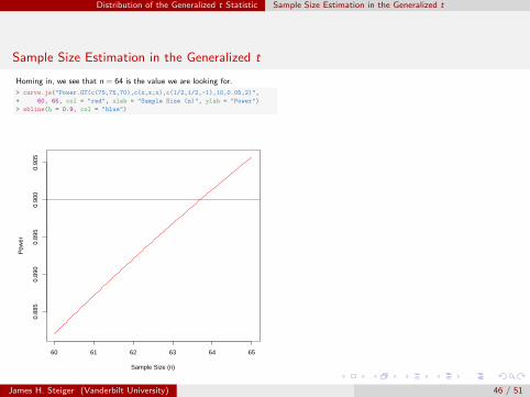
Sample Size Estimation in the Generalized t
Homing in, we see that n = 64 is the value we are looking for.
> curve.js("Power.GT(c(75,75,70),c(x,x,x),c(1/2,1/2,-1),10,0.05,2)",
+ 60, 65, col = "red", xlab = "Sample Size (n)", ylab = "Power")
> abline(h = 0.9, col = "blue")
60 61 62 63 64 65
0.88
50.
890
0.89
50.
900
0.90
5
Sample Size (n)
Pow
er
James H. Steiger (Vanderbilt University) 46 / 51
Power Analysis via Simulation
Power Analysis via Simulation
Because R has advanced functions for computing distributions, andbecause we know formulas for the noncentrality parameter, we can, as wehave seen, construct power functions easily, and use them to computerequired sample size.
However, suppose we needed to compute power for the 1-Sample t and wehad no idea what the non-null distribution of the test statistic is.Presumably, we know the null distribution, otherwise we wouldn’t be usingthe test statistic.
How could we then proceed to perform power calculation and/or samplesize estimation?
James H. Steiger (Vanderbilt University) 47 / 51
Power Analysis via Simulation
Power Analysis via Simulation
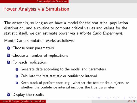
The answer is, so long as we have a model for the statistical populationdistribution, and a routine to compute critical values and values for thestatistic itself, we can estimate power via a Monte Carlo Experiment.
Monte Carlo simulation works as follows:
1 Choose your parameters
2 Choose a number of replications
3 For each replication:
1 Generate data according to the model and parameters
2 Calculate the test statistic or confidence interval
3 Keep track of performance, e.g., whether the test statistic rejects, orwhether the confidence interval includes the true parameter
4 Display the results
James H. Steiger (Vanderbilt University) 48 / 51
Power Analysis via Simulation
Power Analysis via Simulation
There is an introduction to Monte Carlo simulation in Lab 04 ofPsychology 310.
Here, we write a brief program to estimate the power of a 1 sample t test,based on an input value of Es , n, and α. We’ll assume that the situation isthe same as earlier in the lecture. We have a 1-sided null hypothesis thatµ ≤ 70, with the true situation that µ = 75 and σ = 10. What is thepower if n = 25?
James H. Steiger (Vanderbilt University) 49 / 51
Power Analysis via Simulation
Power Analysis via Simulation
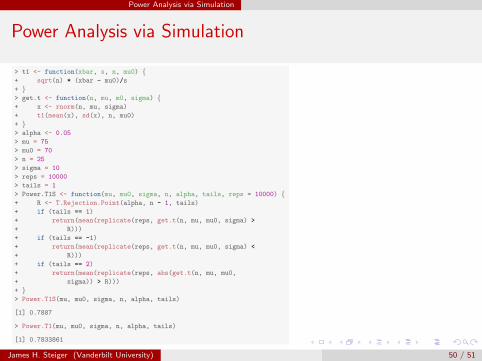
> t1 <- function(xbar, s, n, mu0) {+ sqrt(n) * (xbar - mu0)/s
+ }> get.t <- function(n, mu, m0, sigma) {+ x <- rnorm(n, mu, sigma)
+ t1(mean(x), sd(x), n, mu0)
+ }> alpha <- 0.05
> mu = 75
> mu0 = 70
> n = 25
> sigma = 10
> reps = 10000
> tails = 1
> Power.T1S <- function(mu, mu0, sigma, n, alpha, tails, reps = 10000) {+ R <- T.Rejection.Point(alpha, n - 1, tails)
+ if (tails == 1)
+ return(mean(replicate(reps, get.t(n, mu, mu0, sigma) >
+ R)))
+ if (tails == -1)
+ return(mean(replicate(reps, get.t(n, mu, mu0, sigma) <
+ R)))
+ if (tails == 2)
+ return(mean(replicate(reps, abs(get.t(n, mu, mu0,
+ sigma)) > R)))
+ }> Power.T1S(mu, mu0, sigma, n, alpha, tails)
[1] 0.7887
> Power.T1(mu, mu0, sigma, n, alpha, tails)
[1] 0.7833861
James H. Steiger (Vanderbilt University) 50 / 51
Power Analysis via Simulation
Power Analysis via Simulation
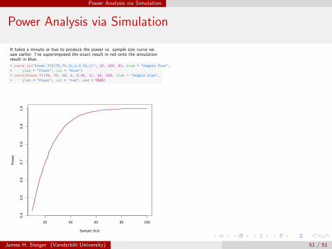
It takes a minute or two to produce the power vs. sample size curve wesaw earlier. I’ve superimposed the exact result in red onto the simulationresult in blue.
> curve.js("Power.T1S(75,70,10,x,0.05,1)", 10, 100, 91, xlab = "Sample Size",
+ ylab = "Power", col = "blue")
> curve(Power.T1(75, 70, 10, x, 0.05, 1), 10, 100, xlab = "Sample Size",
+ ylab = "Power", col = "red", add = TRUE)
20 40 60 80 100
0.4
0.5
0.6
0.7
0.8
0.9
1.0
Sample Size
Pow
er
James H. Steiger (Vanderbilt University) 51 / 51