Embed Size (px)
Citation preview
N. GREGORY MANKIW Harvard University
The Term Structure of
Interest Rates Revisited
THE RELATIONSHIP between long-term and short-term interest rates is crucial for macroeconomic policy evaluation. Since the short-term interest rate is the opportunity cost of holding money, it is widely believed that the Federal Reserve has more direct control over short- term than over long-term interest rates in the United States. Yet if capital is costly to adjust or takes time to place into use, investment decisions may depend on long-term interest rates. The term structure of interest rates thus appears central to the monetary transmission mechanism. Unfortunately, the determinants of the term structure remain poorly understood.
This paper uses data from the United States, Canada, the United Kingdom, and Germany to examine various hypotheses regarding the term structure. My goal is to see whether the experiences of these four countries since 1960 can help provide a general explanation of the term structure. In the United States many observers believe the large varia- .tions in the long-term interest rate since 1979 are not adequately explained by movements in short-term interest rates. Of particular interest is whether the experience of the United States in these and earlier years merely reflects an unusual historical episode.' If it does, it would be
I am grateful to James Poterba, Andrei Shleifer, and members of the Brookings Panel for helpful discussions, and to Miles Kimball for excellent research assistance and discussions.
1. See the comments by Lawrence Weiss on N. Gregory Mankiw and Lawrence H. Summers, "Do Long-Term Interest Rates Overreact to Short-Term Interest Rates?" BPEA, 1:1984, pp. 243-47. Weiss suggests that the U.S. experience since the early 1960s may be anomalous.
61

62 Brookings Papers on Economic Activity, 1:1986
inappropriate to draw any general conclusions from this experience or to extrapolate this experience into the future.
This study is in part motivated by apparent differences between recent experience in the United States and experience elsewhere. In 1985, the rate on long-term government bonds in the United States exceeded the rate on three-month Treasury bills by more than 300 basis points. By contrast, the long-term interest rate in the United Kingdom was more than 100 basis points below the short-term interest rate. Interpreting such divergent national experiences is the primary purpose of studying the term structure more generally.
The most prevalent explanation of the term structure is the expecta- tions theory, which posits that the expected holding returns on bonds of different maturities are equalized, or that they differ by constant term premiums.2 The theory implies that long rates depend on current and expected short rates. The slope of the yield curve, the spread between long rates and short rates, reflects the market's forecast of changes in interest rates. According to the expectations theory, market participants must have expected interest rates to rise in the United States and fall in the United Kingdom.
The test of the expectations theory entails examining whether a steeply sloped yield curve portends an increase in interest rates. Of course, market expectations need not always be realized, since new developments may intercede. Under the assumption of rational expec- tations, however, the expectations theory implies that a steeply sloped yield curve should on average signal an increase in interest rates. In one of the earliest discussions of the expectations theory in 1938, Frederick Macaulay described this implication but asserted that "experience is more nearly the opposite."3
2. For discussions of the expectations theory, see Robert J. Shiller, "The Volatility of Long-Term Interest Rates and Expectations Models of the Term Structure," Journal of Political Economy, vol. 87 (December 1979), pp. 1190-1219; Robert J. Shiller, John Y. Campbell, and Kermit L. Schoenholtz, "Forward Rates and Future Policy: Interpreting the Term Structure of Interest Rates," BPEA, 1:1983, pp. 173-217; and Mankiw and Summers, "Do Long-Term Interest Rates Overreact?" For a review of the older literature on the expectations theory, see Reuben A. Kessel, The Cyclical Behavior of the Term Structure of Interest Rates (National Bureau of Economic Research, 1965).
3. Frederick R. Macaulay, Some Theoretical Problems Suggested by the Movements of Interest Rates, Bond Yields and Stock Prices in the United States Since 1856 (National Bureau of Economic Research, 1938), p. 33.
N. Gregoty Mankiw 63
Experience continues to be intransigent. The data I examine here provide only partial support for the expectations theory. Whenever the long-term government bond rate has greatly exceeded the three-month interest rate, the short rate has indeed tended subsequently to rise; the long rate, however, has not. In fact, to the extent that the slope of the yield curve forecasts long rates at all, it does so in the direction opposite to the one predicted by the theory.
Fluctuations in the slope of the yield curve therefore largely reflect changes in the term premium-the extra return markets provide on long- term, compared with short-term, debt. Without an explicit theory of the term premium, however, this characterization of the data has limited value. In the last part of the paper I therefore turn to two leading theories of the term premium to examine whether changes in perceived risk or changes in relative asset supplies, such as those triggered by debt management policy, could plausibly explain the failure of the expecta- tions theory. Neither theory seems able to explain observed interest rate fluctuations.
A First Look at the Data
This section presents a preliminary examination of the data analyzed in the remainder of this paper. I present some notation and definitions, discuss sample statistics with an eye toward the similarities and differ- ences among countries, and examine fluctuations in the term structure during the 1980s.
NOTATION AND DEFINITIONS
Let r, denote the short-term interest rate and R, denote the long-term interest rate. In particular, r, is the one-period yield, such as the three- month Treasury bill rate in quarterly data, and R, is the yield on a long- term coupon bond, such as the ten- or twenty-year government bond rate. Throughout this paper I approximate the long-term bond as a consol, that is, an infinitely lived security paying a fixed coupon each period.
If P, is the price of a consol paying $1.00 each period, the yield on the
64 Brookings Papers on Economic Activity, 1:1986
consol is defined as
For example, if the infinite stream of payments costs $20.00, the long- term interest rate is 0.05, or 5 percent; $20.00 invested today generates 0.05 x $20.00 = $1.00 each period hereafter. For some purposes it is more useful to use the price of the consol; for others, the yield.
It is important to distinguish between a bond's yield and its holding return. The holding return is the return one receives from buying the bond in one period, holding it until the next period, and selling it for the prevailing price. For a one-period interest rate, the yield and the holding return are identical, since the bond matures in the second period. Hence, rt refers here to both the yield and the holding return on a short-term bond.
Let Ht denote the holding return on a consol between period t and period t + 1. By holding the consol for one period an investor receives the $1.00 coupon payment and the capital gain of Pt+,1 - Pt. Therefore, the holding return is
1 + Pt+1 -Pt (2) H,= Pt
The holding return can also be expressed in terms of the yield using equation 1:
(3) H,--Rt,- RtI
For some purposes, it is useful to consider the following linearized expression for the holding return:
(4) H, R - p
where p is a constant equaling an average long rate. If the long-term interest rate remains unchanged between t and t + 1,
the holding return equals the yield. If the long rate rises, the investor realizes a capital loss on the bond, and the holding return is less than the yield. Similarly, if the long rate falls, the investor realizes a capital gain, and the holding return exceeds the yield.
N. Gregory Mankiw 65
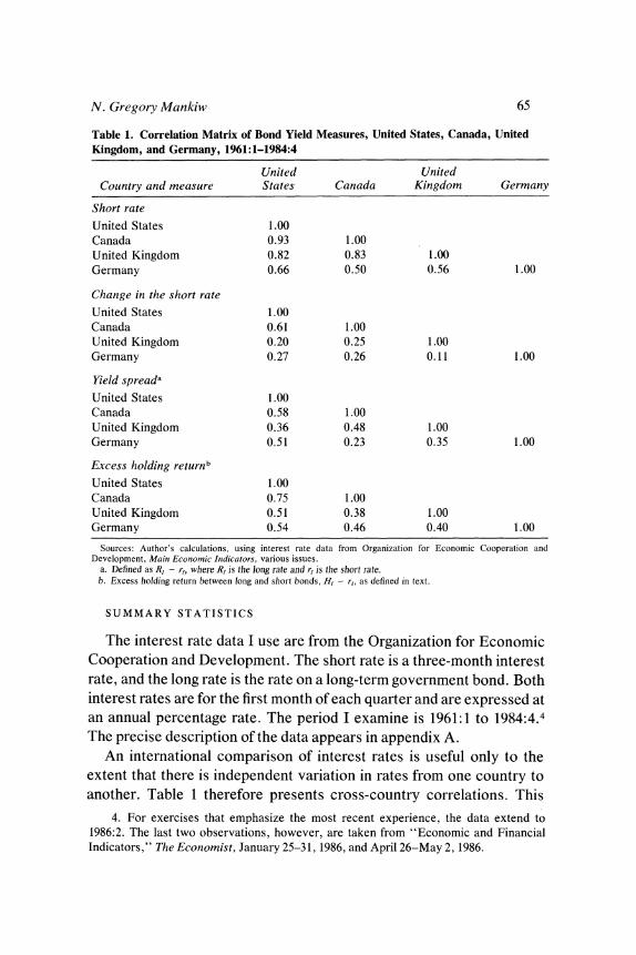
Table 1. Correlation Matrix of Bond Yield Measures, United States, Canada, United Kingdom, and Germany, 1961:1-1984:4
United United Country and measure States Canada Kingdom Germany
Short rate
United States 1.00 Canada 0.93 1.00 United Kingdom 0.82 0.83 1.00 Germany 0.66 0.50 0.56 1.00
Change in the short rate
United States 1.00 Canada 0.61 1.00 United Kingdom 0.20 0.25 1.00 Germany 0.27 0.26 0.11 1.00
Yield spreada
United States 1.00 Canada 0.58 1.00 United Kingdom 0.36 0.48 1.00 Germany 0.51 0.23 0.35 1.00
Excess holding returnb
United States 1.00 Canada 0.75 1.00 United Kingdom 0.51 0.38 1.00 Germany 0.54 0.46 0.40 1.00
Sources: Author's calculations, using interest rate data from Organization for Economic Cooperation and Development, Main Econiomnic Indicators, various issues.
a. Defined as R, - r,, where R, is the long rate and r, is the short rate. b. Excess holding return between long and short bonds, H, - r,, as defined in text.
SUMMARY STATISTICS
The interest rate data I use are from the Organization for Economic Cooperation and Development. The short rate is a three-month interest rate, and the long rate is the rate on a long-term government bond. Both interest rates are for the first month of each quarter and are expressed at an annual percentage rate. The period I examine is 1961:1 to 1984:4.4 The precise description of the data appears in appendix A.
An international comparison of interest rates is useful only to the extent that there is independent variation in rates from one country to another. Table 1 therefore presents cross-country correlations. This
4. For exercises that emphasize the most recent experience, the data extend to 1986:2. The last two observations, however, are taken from "Economic and Financial Indicators," The Economist, January 25-31, 1986, and April 26-May 2, 1986.
66 Brookings Papers on Economic Activity, 1:1986
table shows that the level of the three-month interest rate is highly correlated across the four countries, but that the quarterly change is not. Because interest rates gradually drifted up in most countries during this period, the quarterly change correlations are more telling. In most cases, this correlation is below 0.3. The sole exception is the correlation between the United States and Canada, but even here, the correlation is only 0.61. In general, therefore, there appears to be substantial inde- pendent movement in interest rates in these four countries.
Table 1 also presents the cross-country correlations of the spread between the long rate and the short rate and of the difference in quarterly holding return between the long bond and the short bond. These correlations, generally in the neighborhood of 0.5, show enough inde- pendent variation to warrant a comparison of the term structures of the four countries.
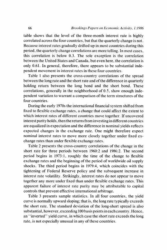
During the early 1970s the international financial system shifted from fixed to flexible exchange rates, a change that could affect the extent to which interest rates of different countries move together. If uncovered interest parity holds, then the returns from investing in different countries are equalized in expectation and the difference in nominal yields reflects expected changes in the exchange rate. One might therefore expect nominal interest rates to move more closely together under fixed ex- change rates than under flexible exchange rates.
Table 2 presents the cross-country correlations of the change in the short rate for three periods between 1960:2 and 1986:2. The second period begins in 1973:1, roughly the time of the change to flexible exchange rates and the beginning of the period of worldwide oil supply shocks. The third period begins in 1979:4, which coincides with the tightening of Federal Reserve policy and the subsequent increase in interest rate volatility. Strikingly, interest rates do not appear to move together any more under fixed than under flexible exchange rates. This apparent failure of interest rate parity may be attributable to capital controls that prevent effective international arbitrage.
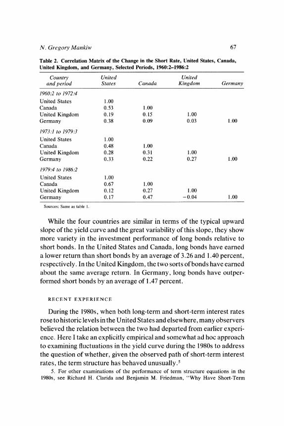
Table 3 presents sample statistics. In all four countries, the yield curve is normally upward sloping; that is, the long rate typically exceeds the short rate. The standard deviation of the long-short spread is also substantial, however, exceeding 100 basis points in each country. Hence, an "inverted" yield curve, in which case the short rate exceeds the long rate, is not especially unusual in any of these countries.
N. Gregoty Mankiw 67
Table 2. Correlation Matrix of the Change in the Short Rate, United States, Canada, United Kingdom, and Germany, Selected Periods, 1960:2-1986:2
Country United United and period States Canada Kingdom Germany
1960:2 to 1972:4 United States 1.00 Canada 0.53 1.00 United Kingdom 0.19 0.15 1.00 Germany 0.38 0.09 0.03 1.00
1973:1 to 1979:3 United States 1.00 Canada 0.48 1.00 United Kingdom 0.28 0.31 1.00 Germany 0.33 0.22 0.27 1.00
1979:4 to 1986:2 United States 1.00 Canada 0.67 1.00 United Kingdom 0.12 0.27 1.00 Germany 0.17 0.47 - 0.04 1.00
Sources: Same as table 1.
While the four countries are similar in terms of the typical upward slope of the yield curve and the great variability of this slope, they show more variety in the investment performance of long bonds relative to short bonds. In the United States and Canada, long bonds have earned a lower return than short bonds by an average of 3.26 and 1.40 percent, respectively. In the United Kingdom, the two sorts of bonds have earned about the same average return. In Germany, long bonds have outper- formed short bonds by an average of 1.47 percent.
RECENT EXPERIENCE
During the 1980s, when both long-term and short-term interest rates rose to historic levels in the United States and elsewhere, many observers believed the relation between the two had departed from earlier experi- ence. Here I take an explicitly empirical and somewhat ad hoc approach to examining fluctuations in the yield curve during the 1980s to address the question of whether, given the observed path of short-term interest rates, the term structure has behaved unusually.5
5. For other examinations of the performance of term structure equations in the 1980s, see Richard H. Clarida and Benjamin M. Friedman, "Why Have Short-Term
~~~~~ t.- rq t-- O C
o t coo
g X t q ̂ tz
o N 0
i~~~~~C C) t-
o : ooo
. o N
;~~~~r 0 b O 00 0ct-
f
cu~~~~~~~~~~~~~c
m X :;oo4
;E 910 U U o
68
N. Gregory Mankiw 69
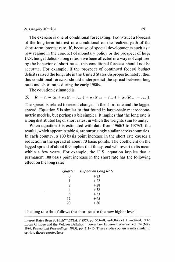
The exercise is one of conditional forecasting. I construct a forecast of the long-term interest rate conditional on the realized path of the short-term interest rate. If, because of special developments such as a new regime in the conduct of monetary policy or the prospect of huge U.S. budget deficits, long rates have been affected in a way not captured by the behavior of short rates, this conditional forecast should not be accurate. For example, if the prospect of continued federal budget deficits raised the long rate in the United States disproportionately, then this conditional forecast should underpredict the spread between long rates and short rates during the early 1980s.
The equation estimated is
(5) Rt - rt= xo + xt (rt - rt-1) + Ox2(rt l - rt_2) + x3 (Rt-I - rt-1).
The spread is related to recent changes in the short rate and the lagged spread. Equation 5 is similar to that found in large-scale macroecono- metric models, but perhaps a bit simpler. It implies that the long rate is a long distributed lag of short rates, in which the weights sum to unity.
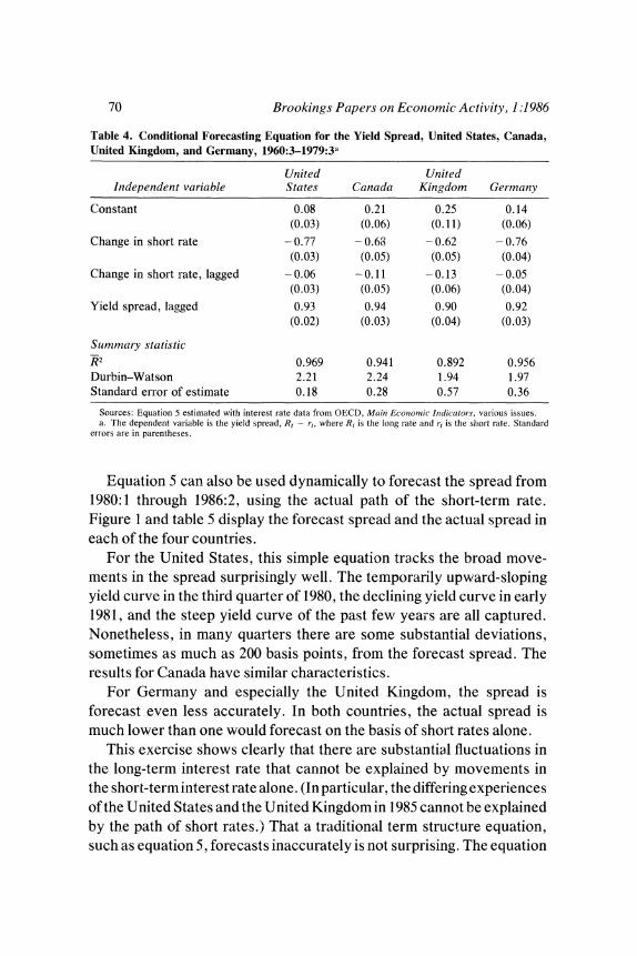
When equation 5 is estimated with data from 1960:3 to 1979:3, the results, which appear in table 4, are surprisingly similar across countries. In each country, a 100 basis point increase in the short rate causes a reduction in the spread of about 70 basis points. The coefficient on the lagged spread of about 0.9 implies that the spread will revert to its mean within a few years. For example, the U.S. equation implies that a permanent 100 basis point increase in the short rate has the following effect on the long rate:
Quarter Impact on Long Rate
0 +23 1 +22 2 +28 4 +38 8 +53
12 +65 20 +80
The long rate thus follows the short rate to the new higher level.
Interest Rates Been So High?" BPEA, 2:1983, pp. 553-78; and Olivier J. Blanchard, "The Lucas Critique and the Volcker Deflation," American Economic Review, vol. 74 (May 1984, Papers and Proceedings, 1983), pp. 211-15. These studies obtain results similar in spirit to those reported here.
70 Brookings Papers on Economic Activity, 1:1986
Table 4. Conditional Forecasting Equation for the Yield Spread, United States, Canada, United Kingdom, and Germany, 1960:3-1979:3a
United United Independent variable States Canada Kingdom Germany
Constant 0.08 0.21 0.25 0.14 (0.03) (0.06) (0.11) (0.06)
Change in short rate - 0.77 - 0.68 - 0.62 - 0.76 (0.03) (0.05) (0.05) (0.04)
Change in short rate, lagged - 0.06 -0.11 -0.13 - 0.05 (0.03) (0.05) (0.06) (0.04)
Yield spread, lagged 0.93 0.94 0.90 0.92 (0.02) (0.03) (0.04) (0.03)
Summary statistic W2 0.969 0.941 0.892 0.956 Durbin-Watson 2.21 2.24 1.94 1.97 Standard error of estimate 0.18 0.28 0.57 0.36
Sources: Equation 5 estimated with interest rate data from OECD, Maini Ecotnotmiic Indicators, various issues. a. The dependent variable is the yield spread, R, - r1, where RI is the long rate and r1 is the sliort rate. Standard
errors are in parentheses.
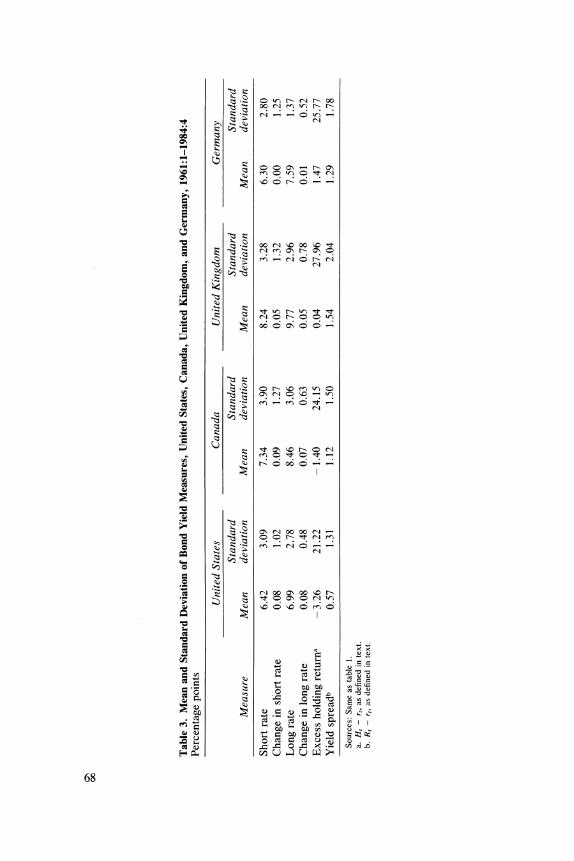
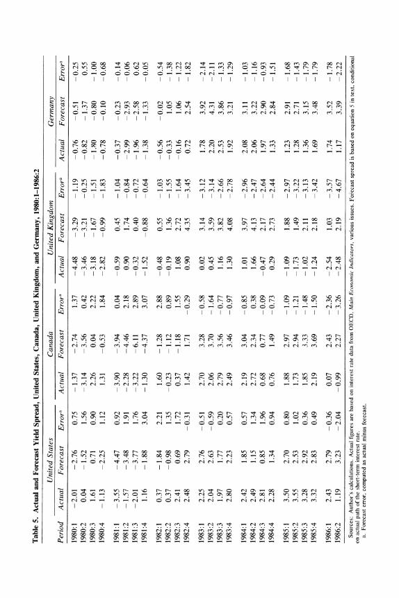
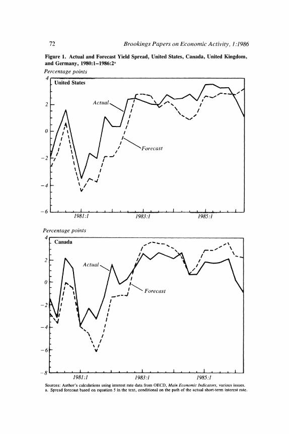
Equation 5 can also be used dynamically to forecast the spread from 1980:1 through 1986:2, using the actual path of the short-term rate. Figure 1 and table 5 display the forecast spread and the actual spread in each of the four countries.
For the United States, this simple equation tracks the broad move- ments in the spread surprisingly well. The temporarily upward-sloping yield curve in the third quarter of 1980, the declining yield curve in early 1981, and the steep yield curve of the past few years are all captured. Nonetheless, in many quarters there are some substantial deviations, sometimes as much as 200 basis points, from the forecast spread. The results for Canada have similar characteristics.
For Germany and especially the United Kingdom, the spread is forecast even less accurately. In both countries, the actual spread is much lower than one would forecast on the basis of short rates alone.
This exercise shows clearly that there are substantial fluctuations in the long-term interest rate that cannot be explained by movements in the short-term interest rate alone. (In particular, the differing experiences of the United States and the United Kingdom in 1985 cannot be explained by the path of short rates.) That a traditional term structure equation, such as equation 5, forecasts inaccurately is not surprising. The equation
V) r o o CI C\ W) n C) ) C) ) N rn 0 q r - 0C
c rq ) 00 r- N lc 0 lc n lc CI 0 C) n CI 00 lc r- rn rn 00 lc C
C t t rq "t rn v) "t v) rq Nt Nc 0 Nc r- :t I< r-- rq rq r--
C\ C- CO 00 v) c rq v) t C\ CIA 00 0 - rn r- 00 C\b^ 00 rn C\tb
> C)~~~~~~~~~~~~~~~~~~~~~~~~~~~~ 00 (4 00 rq C\ C) rq rq 00 C\ t 00 ) rq v) tc C) Nc r- C\ C\ rq , ,t ,O N
0o0 v) C\ O v) ,t C) Cb ) ,t C) c t rq 5 r- c CA )-t
;Y- k- CI "t I <tO 00 C\ r- 0 C\ v) C\ 00 t r- r- v) 00 C\rn C 00 C) oc (
=~~~~~~~~~~~- .0 CA 00 00 C) c t b t r- C\ r- b O obt C\ t
g~~~~~~~~~~~~r r- Oq r- v) O, O Ot C) r- ^t C\ C\ N c N N L, rq rn C)C > l l l l l q
Q~~~~~~~~C .0 OqC )r - q C cC \C q0 c 0 nV \r-C rn rqr \U qr c r n " - ) - t r- ~ - 0r-0 )(
= X ? X ~rq n rq O XoX <6 6 CD (Z; Z tt
ec _q r t 00 r- 00 ^ t O0 C\ C\ tc r- OC\ ObON . . . . . . . . . . . . . . . . . . . . . . . . . .
CA CA t n On O A OA OA OA O A OA O
O CAl _<
f.j
X k b (N N t t X o b X o < o X t b b < X o ^ o A o ?
0 ov 00 0 00 oo o0 oo o0 oo oo 0 00 0 00 00 0 oo 00 o0 00 o0 00 00 00
72 Brookings Papers on Economic Activity, 1:1986
Figure 1. Actual and Forecast Yield Spread, United States, Canada, United Kingdom, and Germany, 1980:1-1986:2a
Percentage points 4
United States
2g A~~~~ct Xa 2
-2 > \\u\/ Forecast
-4 _ I
6~~~
1981:1 1983.1 1985:1
Percentage points 4
Canada 0 ft.
2- Actual
-2 1
NJ~~
-6 v
-8 . 1981 :1 1983:1 1985 :1
Sources: Author's calculations using interest rate data from OECD, Main Economic Indicators, various issues. a. Spread forecast based on equation 5 in the text, conditional on the path of the actual short-term interest rate.
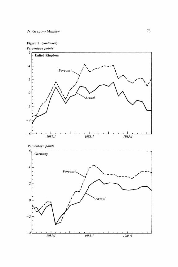
N. Gregory Mankiw 73
Figure 1. (continued)
Percentage points 6
United Kingdom
4 A
Percentage points
6 Germanyl
Forecast
2
0
- 2 _ < , , , / ~~ActAl ta -2
-4 I. I . . I . 1981.1 1983:1 1985:1
74 Brookings Papers on Economic Activity, 1:1986
takes little account of factors, such as the policy environment, that shape investors' expectations, which in turn are crucial to the determination of the long rate.6 In the remainder of this paper, therefore, I examine hypotheses tied more closely to economic theory in an attempt to shed light on the determinants of the term structure.
The Expectations Theory of the Term Structure
In this section I examine the expectations theory of the term structure. To anticipate the results, the data for all four countries appear inconsis- tent with the theory. In particular, the spread between the long-term interest rate and the short-term interest rate is positively related to the subsequent excess return on the long-term bond. In appendix B, I discuss whether measurement error can plausibly explain this finding and conclude that it probably cannot.
Define the term premium as the expected difference between the holding return on a long bond and the holding return on a short bond. That is,
(6) Ot-Et(Ht-rt)
where Et represents the expectation conditional on information available at time t. The term premium represents the extra return expected for holding the long-term asset rather than the short-term asset. It is instructive to write equation 6 in terms of yields using equation 4. Simple rearrangement shows that
(7) Rt- rtR)(EtRt+p-Rt)p + Ot.
The spread between the long rate and the short rate reflects both the expected change in the long rate and the term premium.
If the expectation is removed from equation 6, the difference between the actual holding returns can be written as the sum of the term premium and the expectation error. That is,
(8) Ht-rt Ot+ut+1,
6. This is merely an application of the Lucas critique. Robert E. Lucas, Jr., "Econometric Policy Evaluation: A Critique," in Karl Brunner and Allan H. Meltzer, eds., The Phillips Curve and Labor Markets, Carnegie-Rochester Conference Series on Public Policy, vol. 1 (Amsterdam: North-Holland, 1976), pp. 19-46.
N. Gregory Mankiw 75
where v+ 1 is the difference between the actual and expected returns on the long bond. As equation 4 shows, it represents the "news" about the long rate. In particular,
(9) _t+ _ ~ (Rt +i-pEtRt+ 1)p
Equation 8 merely decomposes the difference in holding return into the anticipated component, the term premium, and the unanticipated com- ponent, the expectation error.
FORECASTING EXCESS RETURNS
The expectations theory of the term structure is the hypothesis that the term premium, Ot, is constant through time. To make this hypothesis operational, I combine it with the hypothesis that expectations are rational, that is, that the expectation error, vt+ 1, is not forecastable with information available at time t. This joint hypothesis implies that the excess holding return,
(10) Ht - rt 0 + ut+ 1,
is not forecastable using variables known at time t. A standard test of the expectations theory is to regress the excess return on any such variable and to see whether it has the predicted coefficient of zero. That is, one estimates
(11) Ht-rt = (x + 13Xt + ut+I
and tests the null hypothesis that X = 0. The theory thus provides a large array of potential tests. Indeed, there
is almost no end to the list of variables that can be tried on the right-hand side of equation 11 in an attempt to invalidate the theory. One should thus be wary when interpreting any reported rejection. Given a sufficient number of attempts, some variable is bound to produce a "significant" rejection. Of course, a finding attributable to such data mining is not truly significant; instead, the t-statistics should be discounted according to the number of unsuccessful attempts at rejecting the theory.
Perhaps a better strategy is to limit the number of tests of the theory. In particular, one might limit the number of candidate Xt variables to those that, if the expectations theory were false, might reasonably be expected to forecast excess returns.
76 Brookings Papers on Economic Activity, 1:1986
One variable that might forecast the excess return is lagged values of the excess return. Since lagged values of vt+I are known at time t, the excess return is serially uncorrelated under the expectations theory. By contrast, if the term premium varied through time (depending on some business-cycle variable, for example), it would plausibly be serially correlated. Equation 8 suggests that such serial correlation in the term premium would appear in the excess return.
A second variable that would plausibly forecast the excess return is the spread between the long rate and the short rate, Rt - rt. Equation 7 suggests that variation in the term premium would be reflected in this spread. A natural test is to use the spread as the forecasting variable in equation 1 1.7
THE PREDICTIVE POWER OF THE SPREAD
The implication of the theory discussed above is a negative one: excess returns should not be forecastable. One can reexpress the theory in a more positive way. In particular, when equation 10 is written in terms of yields using equation 4, it becomes:
(12) Rt+I-Rt = -pO + p(Rt - rt) - pvt+,
that is, the spread between the long rate and the short rate-the slope of the yield curve-should forecast the change in the long-term interest rate. If the yield curve is steeply sloped, the long rate should on average rise; if the yield curve is relatively flat or negatively sloped, the long rate should on average fall. A standard test of the theory is to regress the change in the long rate on the spread to see if the spread accurately signals changes in the long rate.
7. A word about the statistical theory underlying this sort of test: since the null hypothesis (the expectations theory) implies that X, and , +l are uncorrelated, one can use ordinary least squares when estimating equation 11. The justification of the use of the t- statistic to test the null hypothesis, however, is based on asymptotic distribution theory. The crucial question is whether the asymptotic distribution provides a good approximation in typical sample sizes, such as one hundred quarterly observations. Monte Carlo experiments I have done with Matthew Shapiro show that if X, is highly autocorrelated (close to a random walk), one tends to reject the null hypothesis too often. The excess return and the spread are not so highly autocorrelated, however. I therefore rely on the accuracy of the asymptotic distributions throughout this paper. See N. Gregory Mankiw and Matthew D. Shapiro, "Do We Reject Too Often? Small Sample Properties of Tests of Rational Expectations Models," Economics Letters, vol. 20 (January 1986), pp. 139-45.
N. Gregory Mankiw 77
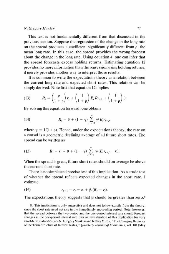
This test is not fundamentally different from that discussed in the previous section. Suppose the regression of the change in the long rate on the spread produces a coefficient significantly different from p, the mean long rate. In this case, the spread provides the wrong forecast about the change in the long rate. Using equation 4, one can infer that the spread forecasts excess holding returns. Estimating equation 12 provides no more information than the regression using holding returns; it merely provides another way to interpret those results.
It is common to write the expectations theory as a relation between the current long rate and expected short rates. This relation can be simply derived. Note first that equation 12 implies
(13) Rt (1P)rt +(1 Et R t+l (1 + .
By solving this equation forward, one obtains
(14) Rt= 0 + (1 - y) >E yiEtrt+j, j = o
where y = 1/(1 + p). Hence, under the expectations theory, the rate on a consol is a geometric declining average of all future short rates. The spread can be written as
x (15) Rt -rt = 0 + (I1-ay) E: yi(Etrt+j -rt). j = o
When the spread is great, future short rates should on average be above the current short rate.
There is no simple and precise test of this implication. As a crude test of whether the spread reflects expected changes in the short rate, I estimate
(16) rt+I-rt = a + 3 (Rt - rt).
The expectations theory suggests that 3 should be greater than zero.8
8. This implication is only suggestive and does not follow exactly from the theory, since the short rate need not rise in the immediately succeeding period. Note, however, that the spread between the two-period and the one-period interest rate should forecast changes in the one-period interest rate. For an investigation of this implication for very short-term maturities, see N. Gregory Mankiw and Jeffrey Miron, "The Changing Behavior of the Term Structure of Interest Rates," Quarterly Journal of Economics, vol. 101 (May
78 Brookings Papers on Economic Activity, 1:1986
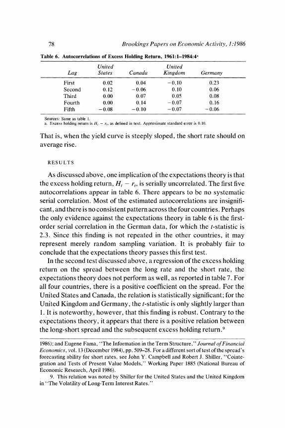
Table 6. Autocorrelations of Excess Holding Return, 1961:1-1984:4a
United United Lag States Canada Kingdom Germany
First 0.02 0.04 -0.10 0.23 Second 0.12 - 0.06 0.10 0.06 Third 0.00 0.07 0.05 0.08 Fourth 0.00 0.14 - 0.07 0.16 Fifth - 0.08 -0.10 - 0.07 - 0.06
Sources: Same as table 1. a. Excess holding return is Ht - rt, as defined in text. Approximate standard error is 0.10.
That is, when the yield curve is steeply sloped, the short rate should on average rise.
RESULTS
As discussed above, one implication of the expectations theory is that the excess holding return, Ht - rt, is serially uncorrelated. The first five autocorrelations appear in table 6. There appears to be no systematic serial correlation. Most of the estimated autocorrelations are insignifi- cant, and there is no consistent pattern across the four countries. Perhaps the only evidence against the expectations theory in table 6 is the first- order serial correlation in the German data, for which the t-statistic is 2.3. Sin-ce this finding is not repeated in the other countries, it may represent merely random sampling variation. It is probably fair to conclude that the expectations theory passes this first test.
In the second test discussed above, a regression of the excess holding return on the spread between the long rate and the short rate, the expectations theory does not perform as well, as reported in table 7. For all four countries, there is a positive coefficient on the spread. For the United States and Canada, the relation is statistically significant; for the United Kingdom and Germany, the t-statistic is only slightly larger than 1. It is noteworthy, however, that this finding is robust. Contrary to the expectations theory, it appears that there is a positive relation between the long-short spread and the subsequent excess holding return.9
1986); and Eugene Fama, "The Information in the Term Structure," Journal of Financial Economics, vol. 13 (December 1984), pp. 509-28. Foradifferent sort of test of the spread's forecasting ability for short rates, see John Y. Campbell and Robert J. Shiller, "Cointe- gration and Tests of Present Value Models," Working Paper 1885 (National Bureau of Economic Research, April 1986).
9. This relation was noted by Shiller for the United States and the United Kingdom in 'The Volatility of Long-Term Interest Rates."
N. Gregory Mankiw 79
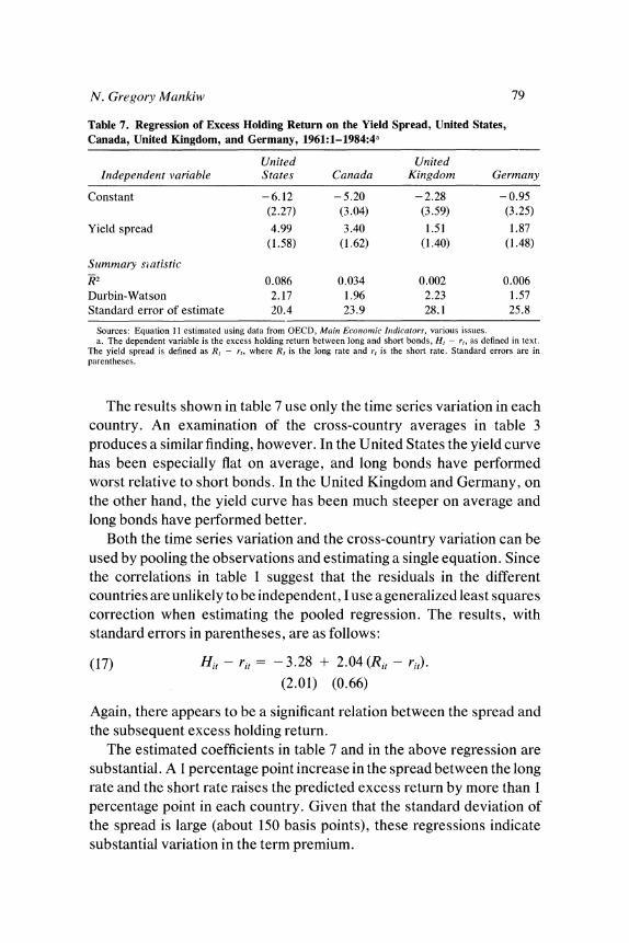
Table 7. Regression of Excess Holding Return on the Yield Spread, United States, Canada, United Kingdom, and Germany, 1961:1-1984:4a
United United Independent variable States Canada Kingdom Germany
Constant - 6.12 - 5.20 - 2.28 - 0.95 (2.27) (3.04) (3.59) (3.25)
Yield spread 4.99 3.40 1.51 1.87 (1.58) (1.62) (1.40) (1.48)
Summary statistic R2 0.086 0.034 0.002 0.006 Durbin-Watson 2.17 1.96 2.23 1.57 Standard error of estimate 20.4 23.9 28.1 25.8
Sources: Equation 11 estimated using data from OECD, Mainz Econiomic Indicators, various issues. a. The dependent variable is the excess holding return between long and short bonds, H, - r,, as defined in text.
The yield spread is defined as R, - rt, where Rt is the long rate and rt is the short rate. Standard errors are in parentheses.
The results shown in table 7 use only the time series variation in each country. An examination of the cross-country averages in table 3 produces a similar finding, however. In the United States the yield curve has been especially flat on average, and long bonds have performed worst relative to short bonds. In the United Kingdom and Germany, on the other hand, the yield curve has been much steeper on average and long bonds have performed better.
Both the time series variation and the cross-country variation can be used by pooling the observations and estimating a single equation. Since the correlations in table 1 suggest that the residuals in the different countries are unlikely to be independent, I use a generalized least squares correction when estimating the pooled regression. The results, with standard errors in parentheses, are as follows:
(17) Hit - rit= - 3.28 + 2.04 (Rit - rit) (2.01) (0.66)
Again, there appears to be a significant relation between the spread and the subsequent excess holding return.
The estimated coefficients in table 7 and in the above regression are substantial. A 1 percentage point increase in the spread between the long rate and the short rate raises the predicted excess return by more than 1 percentage point in each country. Given that the standard deviation of the spread is large (about 150 basis points), these regressions indicate substantial variation in the term premium.
80 Brookings Papers on Economic Activity, 1:1986
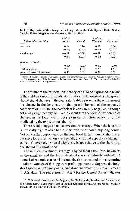
Table 8. Regression of the Change in the Long Rate on the Yield Spread, United States, Canada, United Kingdom, and Germany, 1961:1-1984:4a
United United Independent variable States Canada Kingdom Germany
Constant 0.14 0.16 0.07 0.04 (0.05) (0.08) (0. 10) (0.07)
Yield spread -0.11 - 0.08 - 0.01 - 0.03 (0.04) (0.04) (0.04) (0.03)
Summaty statistic R 2 0.076 0.029 - 0.009 - 0.003 Durbin-Watson 2.10 1.87 2.29 1.63 Standard error of estimate 0.46 0.63 0.79 0.52
Sources: Equation 12 estimated using interest rate data from OECD, Maint Ecotionzic Inidicators, various issues. a. The dependent variable is the change in the long-term interest rate, R,+1 - R,. The yield spread is defined as
Rt - rt. Standard errors are in parentheses.
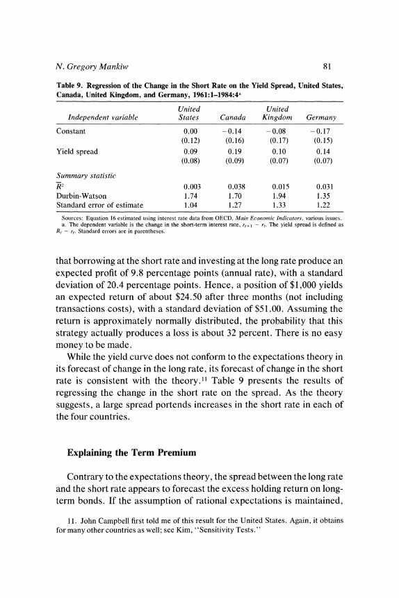
The failure of the expectations theory can also be expressed in terms of the yield on long-term bonds. As equation 12 demonstrates, the spread should signal changes in the long rate. Table 8 presents the regression of the change in the long rate on the spread. Instead of the expected coefficient of p : 0.02, the coefficient is consistently negative, although not always significantly so. To the extent that the yield curve forecasts changes in the long rate, it does so in the direction opposite to that predicted by the expectations theory. 10
These results suggest a naive investment strategy. When the long rate is unusually high relative to the short rate, one should buy long bonds. Not only is the coupon yield on the long bond higher than the short rate, but since long rates will on average fall, one should expect a capital gain as well. Conversely, when the long rate is low relative to the short rate, one should buy short bonds.
The implied investment strategy is by no means risk-free, however, as the small R2 and the large standard error of estimate indicate. A numerical example can best illustrate the risk associated with attempting to take advantage of this apparent profit opportunity. Suppose the long- short spread is 319 basis points, two standard deviations above its mean in U.S. data. The regression in table 7 for the United States indicates
10. This result also obtains for Belgium, the Netherlands, Sweden, and Switzerland. See Harold Kim, "Sensitivity Tests of the Expectations Term Structure Model" (Under- graduate thesis, Harvard University, 1986).
N. Gregory Mankiw 81
Table 9. Regression of the Change in the Short Rate on the Yield Spread, United States, Canada, United Kingdom, and Germany, 1961:1-1984:4a
United United Independent variable States Canada Kingdom Germany
Constant 0.00 -0.14 - 0.08 - 0.17 (0.12) (0.16) (0.17) (0.15)
Yield spread 0.09 0.19 0.10 0.14 (0.08) (0.09) (0.07) (0.07)
Summary statistic
R 2 0.003 0.038 0.015 0.031 Durbin-Watson 1.74 1.70 1.94 1.35 Standard error of estimate 1.04 1.27 1.33 1.22
Sources: Equation 16 estimated using interest rate data from OECD, Maini Econiomic Intdicators, various issues. a. The dependent variable is the change in the short-term interest rate, rt+ - rt. The yield spread is defined as
Rt - rt. Standard errors are in parentheses.
that borrowing at the short rate and investing at the long rate produce an expected profit of 9.8 percentage points (annual rate), with a standard deviation of 20.4 percentage points. Hence, a position of $1,000 yields an expected return of about $24.50 after three months (not including transactions costs), with a standard deviation of $51.00. Assuming the return is approximately normally distributed, the probability that this strategy actually produces a loss is about 32 percent. There is no easy money to be made.
While the yield curve does not conform to the expectations theory in its forecast of change in the long rate, its forecast of change in the short rate is consistent with the theory.11 Table 9 presents the results of regressing the change in the short rate on the spread. As the theory suggests, a large spread portends increases in the short rate in each of the four countries.
Explaining the Term Premium
Contrary to the expectations theory, the spread between the long rate and the short rate appears to forecast the excess holding return on long- term bonds. If the assumption of rational expectations is maintained,
11. John Campbell first told me of this result for the United States. Again, it obtains for many other countries as well; see Kim, "Sensitivity Tests."
82 Brookings Papers on Economic Activity, 1:1986
this finding implies that the term premium varies through time and is positively correlated with this spread.
Of course, to say that the term premium is time-varying is to say no more than that the expectations theory of the term structure fails. Without an explicit theory of the term premium, it is not clear how to make use of this finding. The next step is therefore to seek an explanation for the variation in the term premium.
RISK AS AN OMITTED VARIABLE
Perhaps the most natural explanation of the term premium is that it represents the extrareturn necessary to compensate investors forbearing the extra risk associated with long-term bonds. (As discussed later, the term premium could in principle be negative, in which case investors require compensation for holding short-term bonds.) In this section, I consider various measures of risk to see whether they can help explain the apparent variation in the term premium.
Let RISK be some measure of the risk associated with holding a long- term bond. It is natural to posit that the term premium is positively related to RISK. That is,
(18) 0 ca RISK,.
One would expect that fluctuations in RISK would also be reflected in the spread between the long rate and the short rate, implying that the spread would forecast excess holding returns. In principle, therefore, the hypothesis that there are substantial fluctuations in perceived risk could explain the rejection of the expectations theory reported above.
If RISK were observable, it would be natural to test this hypothesis by estimating the following regression:
(19) Ht-rt = a + a (Rt - rt) + y (RISK).
If the spread forecasts the holding return because it is proxying for RISK, then 3 in this regression should fall to zero when RISK is explicitly included.
A necessary condition for RISK to explain the rejection of the expectations theory is that RISKt and Rt - rt be positively correlated. If they are not correlated, then the addition of RISK into the regression will not change the coefficient on the spread. Another test of the risk
N. Gregoiy Mankiw 83
hypothesis, therefore, is to estimate
(20) RISK, = a + a (Rt - r).
The hypothesis predicts that the coefficient on the spread is greater than zero. That is, the long bond is risky when the yield curve is steeply sloped.
Unfortunately, RISK is not observable. We can, however, obtain imperfect proxies for it. Measurement error in RISK will bias the estimates of equation 19 but will not bias the estimates of equation 20 as long as the measurement error is uncorrelated with the spread. For this reason, I restrict my attention to this second implication of the risk hypothesis.
INTEREST RATE VOLATILITY
Holding a short-term bond for one period produces a risk-free nominal return. By contrast, holding a long-term bond for one period produces a highly risky return, since the capital gain depends on the next period's price, Pt+ , or, equivalently, on the next period's long rate, Rt + . The more volatile the long rate, the more risky is the long-term bond. If investors are risk averse, they should require a greater expected return to hold long-term bonds when they are riskier. One might therefore expect greater interest rate volatility to be associated with a greater term premium. 12
A casual examination of the sample statistics in table 3 lends some plausibility to the volatility hypothesis. The standard deviation of the excess holding return is smallest in the United States and greatest in the United Kingdom. As this hypothesis predicts, the average long-short spread is also smallest in the United States and greatest in the United Kingdom. We also see in table 3, however, that the within-country variation in the spread is greater than the across-country variation in
12. This sort of risk measure has been useful in understanding the term structure for maturities of less than one year. For recent examples, see David S. Jones and V. Vance Roley, "Rational Expectations and the Expectations Model of the Term Structure: A Test Using Weekly Data," Journal of Monetat-y Economics, vol. 12 (September 1983), pp. 453- 65; and Robert F. Engle, David M. Lilien, and Russell P. Robins, "Estimating Time Varying Risk Premia in the Term Structure: The ARCH-M Model" (University of California, San Diego, 1985).
84 Brookings Papers on Economic Activity, 1:1986
these sample averages. Before examining whether this hypothesis is consistent with the international evidence, it is natural to examine whether the hypothesis can shed light on the large time series variation in the spread in each of these countries.
Consider one measure of ex post, or actual, volatility:
Pt+?I - P (21) VOLt =
VOL is the absolute value of the percentage change in the price of the long-term bond. Equation 1 can be used to rewrite equation 21 as
(22) VOLt = | - Rt+ I
Hence, VOLt also measures the absolute percentage change in the long rate. A plausible model is that the relevant measure of RISK is ex ante, or expected, volatility. That is,
(23) RISKt c' Et (VOLe).
If expected volatility were observable, then the tests could proceed as discussed above.
Any test of this volatility hypothesis must take into account the fact that expected volatility is not directly observable. Actual volatility, however, is observable and can be viewed as an imperfect proxy for expected volatility. The rational expectations hypothesis implies that the measurement error-the difference between actual and expected volatility-is uncorrelated with the spread at time t.
I therefore test the volatility hypothesis by examining the relation between the long-short spread and actual volatility. I estimate
(24) VOLt = a + a (Rt - rt).
If the spread is proxying for expected volatility, then it should be positively related to actual volatility. Hence, the volatility hypothesis predicts that 3 is greater than zero. 13
13. Note, however, that there will be much variation in actual volatility that is not forecastable. Hence, the R2 in this regression is not expected to be large.
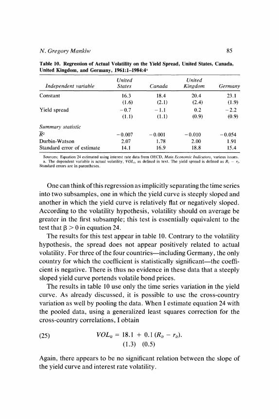
N. Gregory Mankiw 85
Table 10. Regression of Actual Volatility on the Yield Spread, United States, Canada, United Kingdom, and Germany, 1961:1-1984:4a
United United Independent variable States Canada Kingdom Germany
Constant 16.3 18.4 20.4 23.1 (1.6) (2.1) (2.4) (1.9)
Yield spread -0.7 -1.1 0.2 -2.2 (1.1) (1.1) (0.9) (0.9)
Summary statistic R 2 - 0.007 - 0.001 -0.010 - 0.054 Durbin-Watson 2.07 1.78 2.00 1.91 Standard error of estimate 14.1 16.9 18.8 15.4
Sources: Equation 24 estimated using interest rate data from OECD, Maint Ecotionoic Intdicators, various issues. a. The dependent variable is actual volatility, VOLt, as defined in text. The yield spread is defined as Rt - rt.
Standard errors are in parentheses.
One can think of this regression as implicitly separating the time series into two subsamples, one in which the yield curve is steeply sloped and another in which the yield curve is relatively flat or negatively sloped. According to the volatility hypothesis, volatility should on average be greater in the first subsample; this test is essentially equivalent to the test that 3 > 0 in equation 24.
The results for this test appear in table 10. Contrary to the volatility hypothesis, the spread does not appear positively related to actual volatility. For three of the four countries-including Germany, the only country for which the coefficient is statistically significant-the coeffi- cient is negative. There is thus no evidence in these data that a steeply sloped yield curve portends volatile bond prices.
The results in table 10 use only the time series variation in the yield curve. As already discussed, it is possible to use the cross-country variation as well by pooling the data. When I estimate equation 24 with the pooled data, using a generalized least squares correction for the cross-country correlations, I obtain
(25) VOLi, = 18.1 + 0.1 (Rit - rit) (1.3) (0.5)
Again, there appears to be no significant relation between the slope of the yield curve and interest rate volatility.
86 Brookings Papers on Economic Activity, 1:1986
CONSUMPTION COVARIABILITY
According to finance theory, the relevant measure of the risk of an asset is its nondiversifiable, or systematic, risk. To the extent that an asset's risk is diversifiable, an investor does not require a greater return to hold that asset. The apparent failure of the volatility hypothesis may be attributable to the fact that it does not distinguish between diversifiable and nondiversifiable risk.
Much recent work has used the consumption-based capital asset pricing model to link product markets and financial markets.14 The consumption CAPM implies that the expected excess return on an asset depends on its covariability with consumption growth. In particular, it implies
(26) Ot Et (Ht - rt) = A cov (Ht - rt, Ct+Il / Ct),
where C is consumption, A is the coefficient of relative risk aversion of the typical investor, and cov denotes the conditional covariance.15 If long bonds earn a high return when consumption falls, then long bonds are a hedge against bad times. In this case, investors do not need an incentive to hold long bonds; the term premium is low or negative. Similarly, if long bonds earn a low return when consumption falls, then holding long bonds exacerbates consumption risk, in which case inves- tors require a large term premium.
Depending on the source of the shocks hitting the economy, it is possible to imagine that long bonds have either positive or negative consumption covariability. Positive shocks to productivity would plau- sibly raise interest rates through investment demand and raise consump-
14. See Lars Peter Hansen and Kenneth J. Singleton, "Stochastic Consumption, Risk Aversion, and the Temporal Behavior of Asset Returns," Journal of Political Economy, vol. 91 (April 1983), pp. 249-65; Robert J. Shiller, "Consumption, Asset Markets and Macroeconomic Fluctuations," in Karl Brunner and Allan H. Meltzer, eds., Economic Policy in a World of Change, Carnegie-Rochester Conference Series on Public Policy, vol. 17 (Amsterdam: North-Holland, 1982), pp. 203-38; and N. Gregory Mankiw and Matthew D. Shapiro, "Risk and Return: Consumption Beta Versus Market Beta," Review of Economics and Statistics, forthcoming.
15. See Sanford Grossman and Robert J. Shiller, "Consumption Correlatedness and Risk Measurement in Economies with Non-traded Assets and Heterogeneous Informa- tion," Journal of FinancialEconomics, vol. 10 (July 1982), pp. 195-210. More specifically, A is the harmonic mean of investors' coefficient of relative risk aversion.
N. Gregory Mankiw 87
tion through permanent income, implying a negative consumption beta for long bonds. On the other hand, increases in government purchases, to be followed by tax increases, might increase interest rates while reducing consumption, implying a positive consumption beta. Increases in inflation would probably raise nominal interest rates without having any major effect on consumption. There is thus no obvious presumption regarding the size or sign of the consumption covariance. If the source of the shocks changes, this theory predicts that the consumption covar- iance and thus the term premium will change as well.
The testing strategy I propose for this consumption beta model parallels that for the volatility hypothesis. Define the actual consumption covariability as
(27) ccovt [(Ht - rt) - (Ht - rt)][(Ct+1!Ct) - (Ct+1!Ct)],
where a bar over a variable indicates the sample mean. 16 The actual covariability of the excess holding return with consumption growth is measured by ccovt. The consumption beta model suggests that the term premium is proportional to the conditional expectation of ccov. That is,
(28) Ot = A Et(ccovt).
According to this model, the spread forecasts the excess holding return because it is proxying for variation in the consumption beta.
I estimate the following regression:
(29) ccovt = a + a (Rt - rt).
If variation in the consumption beta explains the variation in the term premium reported above, then 3 in equation 29 should be greater than zero. The model has a more specific prediction, however. Since an increase in the spread raises the expected excess holding return by a factor of about 2, the model predicts 3 is about 2/A, where A is again the coefficient of relative risk aversion. Note, however, that because all the data, including consumption growth rates, are measured at a percentage annual rate, a coefficient of 800/A should be expected. Since the coefficient of relative risk aversion is usually thought to be between 0.5 and 8, the theory predicts a coefficient between 100 and 1,600.
16. My use of the sample mean does not take account of variation in the conditional mean of the excess return and consumption growth. Since the predictability (R2) of these two variables is small, this approximation is probably very accurate.
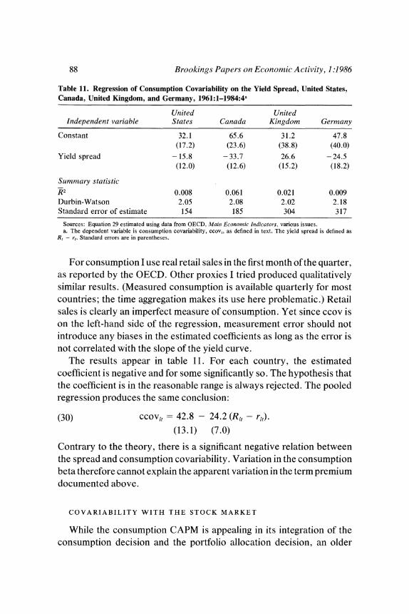
88 Brookings Papers on Economic Activity, 1:1986
Table 11. Regression of Consumption Covariability on the Yield Spread, United States, Canada, United Kingdom, and Germany, 1961:1-1984:4a
United United Independent variable States Canada Kingdom Germany
Constant 32.1 65.6 31.2 47.8 (17.2) (23.6) (38.8) (40.0)
Yield spread - 15.8 - 33.7 26.6 - 24.5 (12.0) (12.6) (15.2) (18.2)
Summary statistic R 2 0.008 0.061 0.021 0.009 Durbin-Watson 2.05 2.08 2.02 2.18 Standard error of estimate 154 185 304 317
Sources: Equation 29 estimated using data from OECD, Mainz Economic Intdicators, various issues. a. The dependent variable is consumption covariability, ccov,, as defined in text. The yield spread is defined as
R, - r,. Standard errors are in parentheses.
For consumption I use real retail sales in the first month of the quarter, as reported by the OECD. Other proxies I tried produced qualitatively similar results. (Measured consumption is available quarterly for most countries; the time aggregation makes its use here problematic.) Retail sales is clearly an imperfect measure of consumption. Yet since ccov is on the left-hand side of the regression, measurement error should not introduce any biases in the estimated coefficients as long as the error is not correlated with the slope of the yield curve.
The results appear in table 11. For each country, the estimated coefficient is negative and for some significantly so. The hypothesis that the coefficient is in the reasonable range is always rejected. The pooled regression produces the same conclusion:
(30) ccovit = 42.8 - 24.2 (Rit - rit) (13.1) (7.0)
Contrary to the theory, there is a significant negative relation between the spread and consumption covariability. Variation in the consumption beta therefore cannot explain the apparent variation in the term premium documented above.
COVARIABILITY WITH THE STOCK MARKET
While the consumption CAPM is appealing in its integration of the consumption decision and the portfolio allocation decision, an older
N. Gregory Mankiw 89
tradition in finance suggests using the covariance with the market return as the appropriate measure of risk. One can view the consumption CAPM as using consumption growth as the ideal proxy for the market return: individuals increase consumption when the return on all their assets, including human capital, has been above normal and decrease their consumption when the return has been below normal. The apparent failure of the consumption CAPM to explain the variation in the term premium, however, leaves open the question of whether some other measure of the market return can more successfully shed light on the term strticture.
Perhaps the most standard measure of risk uses the return on the stock market as the market return. Matthew Shapiro and I examined the return on a cross-section of 464 stocks listed on the New York Stock Exchange. We found that the covariance with the Standard and Poor's index is more related to average return than is the covariance with consumption growth.17 That is, stocks appear to be priced using the more standard market beta rather than the consumption beta. This finding suggests that the covariability of return with a stock market index may better explain fluctuations in the term structure as well.
One possible argument for the use of the market covariance is that the stock market may provide a better measure of the consumption changes of the typical investor than does aggregate consumption. To the extent that aggregate consumption is dominated by individuals who are liquidity constrained, the empirical implementation of the consumption CAPM is called into question. One can view the standard capital asset pricing model as essentially using the stock market index as a proxy for the consumption of the typical investor.
With this interpretation, it is natural to repeat the above test using a stock market index in the place of retail sales. In particular, I replace consumption growth in equation 27 with the excess return on the stock market. The test then proceeds as before.
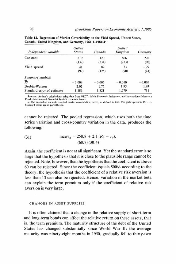
Table 12 contains the results of regressing the actual market covaria- bility (mcov) on the spread. Perhaps the most salient feature of these results is the large standard errors; in no country is the coefficient statistically significant. In three of the four countries, the coefficient is positive, however, and the hypothesis that it is in the plausible range
17. Mankiw and Shapiro, "Risk and Return."
90 Brookings Papers on Economic Activity, 1:1986
Table 12. Regression of Market Covariability on the Yield Spread, United States, Canada, United Kingdom, and Germany, 1961:1-1984:4a
United United Independent variable States Canada Kingdom Germany
Constant 219 120 606 270 (132) (234) (233) (90)
Yield spread 41 82 33 -29
(97) (125) (90) (41)
Summary statistic R2 - 0.009 - 0.006 - 0.010 - 0.005 Durbin-Watson 2.02 1.75 1.95 1.93 Standard error of estimate 1,186 1,821 1,779 711
Sources: Author's calculations using data from OECD, Main Economic Indicators, and International Monetary Fund, International Financial Statistics, various issues.
a. The dependent variable is actual market covariability, mcov,, as defined in text. The yield spread is R, - r,. Standard errors are in parentheses.
cannot be rejected. The pooled regression, which uses both the time series variation and cross-country variation in the data, produces the following:
(31) mcovit = 258.8 + 2.1 (Rit - rit) (68.7) (30.4)
Again, the coefficient is not at all significant. Yet the standard error is so large that the hypothesis that it is close to the plausible range cannot be rejected. Note, however, that the hypothesis that the coefficient is above 60 can be rejected. Since the coefficient equals 800/A according to the theory, the hypothesis that the coefficient of a relative risk aversion is less than 13 can also be rejected. Hence, variation in the market beta can explain the term premium only if the coefficient of relative risk aversion is very large.
CHANGES IN ASSET SUPPLIES
It is often claimed that a change in the relative supply of short-term and long-term bonds can affect the relative return on these assets, that is, the term premium. The maturity structure of the debt of the United States has changed substantially since World War II: the average maturity was ninety-eight months in 1950, gradually fell to thirty-two

N. Gregoty Mankiw 91
months in 1975, and then rose to forty-five months in 1980.18 Such changes can in principle explain fluctuations in the term premium.
While changes in asset supplies might affect the term premium, it is unlikely that they can fully explain the changing term premium implied by the regressions in table 7. First, since the standard deviation of the spread exceeds 150 basis points and the coefficient on the spread is about 2, these regressions imply that the standard deviation of the term premium exceeds 300 basis points. Yet available estimates imply that asset supplies cannot have that great an effect. Using data from 1960 to 1980, Benjamin Friedman estimates that a$ 100 billion shift in government debt from short to long bonds increases the term premium by only 16 basis points. 19 (In 1970, the middle of this period, the total privately held debt was only $217 billion.) Jeffrey Frankel estimates even smaller effects of debt management.20
Second, the maturity structure of the debt changes only gradually. It does not change greatly quarter to quarter or year to year. In contrast, the term premium implied by the results in table 7 fluctuates more quickly. In particular, the eighth autocorrelation of the spread is only slightly larger than zero, implying that a high value of the term premium today does not convey much information on the term premium in eight quarters. If the maturity structure of the public debt were the primary cause of the fluctuating term premium, the term premium would be much more highly serially correlated.
Hence, it appears that the term premium is too volatile and not sufficiently serially correlated to be easily explained by fluctuations in the relative supply of long and short bonds.
Conclusion
As is unfortunately common in economics, more questions remain open than have been resolved. It is easier to show that the expectations
18. Benjamin M. Friedman, "Debt Management Policy, Interest Rates, and Economic Activity" (Harvard University, 1985).
19. Benjamin M. Friedman, "Crowding Out or Crowding In? Evidence on Debt- Equity Substitutability" (Harvard University, 1985).
20. Jeffrey A. Frankel, "Portfolio Crowding-Out Empirically Estimated," Quarterly Journal of Economics, vol. 100 (1985 Supplement), pp. 1041-65.
92 Brookings Papers on Economic Activity, 1:1986
theory of the term structure fails than to explain why. Neither changes in bond price volatility, nor changes in nondiversifiable risk, nor changes in relative asset supplies can satisfactorily explain the apparently large variation in the term premium and thus the failure of the expectations theory.
The elusiveness of an empirically satisfactory explanation for the behavior of the term structure is disappointing. Since the long-term interest rate is probably crucial to the determination of aggregate demand, the inability to account for fluctuations in term structure is all the more frustrating. Developing theoretically plausible and empirically testable theories of the term premium should remain high on the research agenda.
APPENDIX A
Data Description
THIS APPENDIX describes the data used in this paper. All the data are for the first month of each quarter and are from data banks maintained by Data Resources, Inc. Listed below are the sources from which DRI takes the data, along with the description taken from those sources.
Short-Term Interest Rates
Source: Organization for Economic Cooperation and Development, Main Economic Indicators.
United States: Rate on three-month Treasury bills, average of daily rates during the week of the last Monday of the month.
Canada: Rate on three-month Treasury bills, average of last weekly issue in month.
United Kingdom: Rate on ninety-one-day Treasury bills, average rate of allotment on last issue of month.
Germany: Rate on three-month loans (Frankfurt), monthly averages of daily data.
N. Gregory Mankiw 93
Long-Term Interest Rates
Source: Organization for Economic Cooperation and Development, Main Economic Indicators.
United States: Yield on long-term government bonds, ten years and over, monthly averages of daily rates.
Canada: Yield on long-term government bonds, last Wednesday of month.
United Kingdom: Yield on government bonds, 2.5 percent consols, last Friday of month.
Germany: Yield on long-term government bonds.
Stock Prices: Industrial Share Prices
Source: International Monetary Fund, International Financial Sta- tistics.
United States: Laspeyres index of Standard and Poor's Corporation for 400 industrials on the New York Exchange based on daily closing quotations.
Canada: Closing quotations at the end of the month on the Montreal Stock Exchange for sixty-five industrial shares.
United Kingdom: Monthly average of daily quotations of 500 industrial ordinary shares.
Germany: Monthly average of daily quotations covering approxi- mately 95 percent of common shares of industrial companies with headquarters in Germany.
APPENDIX B
Can Measurement Error Explain the Failure of the Expectations Theory?
ONE POSSIBLE EXPLANATION for the rejection of the expectations theory is measurement error in the interest rate data. This problem is potentially
94 Brookings Papers on Economic Activity, 1:1986
important for the long rate. Often long-term interest rates are not inferred directly from the market price of actual bonds, because bonds of the correct maturity may not be available. Instead, the long rate is read off a yield curve that is fit using the bond yields that are available. This interpolation may be a source of measurement error.
The bias that this measurement error induces is consistent with the observed failure of the expectations theory. For instance, if Rt is measured too high, then the measured spread, Rt - rt, will be too high; equation 4 shows that the measured excess holding return, Ht - rt, will be too high as well. Hence, measurement error could induce the positive relation reported in table 7.
A direct test of the measurement error hypothesis is possible. In particular, lagged values of the long-short spread can be used as instru- mental variables to reestimate the regressions in table 7. Two conditions are necessary for this procedure to be valid. First, the lagged spread must be uncorrelated with the measurement error in the current spread, which is the case if the measurement error is serially uncorrelated. (This condition seems a plausible identifying assumption. Below I discuss the possibility of serially correlated measurement error.) Second, the lagged values of the spread must be correlated with the true value of the current spread. This second condition can be checked by examining the adjusted R2 from the first-stage regression (the regression of the current spread on the lagged spreads). The instrumental variable procedure therefore appears a relatively easy way to test for the importance of measurement error in generating the rejections of the expectations theory.
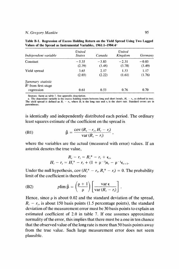
Table B-I presents the regressions from table 7 reestimated with this instrumental variables procedure. The coefficient on the spread remains positive in each case, although usually somewhat smaller. Also in each case the standard error is larger, so the null hypothesis that the coefficient is zero cannot be rejected. While these results are not sufficiently strong to rule out the measurement error hypothesis, neither do they point to measurement error as a likely candidate to explain the failure of the expectations theory reported above.
A second way to gauge the practical importance of measurement error is to calculate directly how much error is necessary to generate the coefficients reported in table 7. Assume that the short rate is measured accurately and that the long rate is subject to measurement error, E, that
N. Gregoty Mankiw 95
Table B-1. Regression of Excess Holding Return on the Yield Spread Using Two Lagged Values of the Spread as Instrumental Variables, 1961:1-1984:4a
United United Independent variable States Canada Kingdom Germany
Constant - 5.35 - 3.83 -2.31 - 0.03 (2.39) (3.48) (3.78) (3.49)
Yield spread 3.65 2.17 1.53 1.17 (2.03) (2.22) (1.61) (1.76)
Summary statistic R2 from first-stage
regression 0.61 0.53 0.76 0.70
Sources: Same as table 7. See appendix description. a. The dependent variable is the excess holding return between long and short bonds, H, - r,, as defined in text.
The yield spread is defined as R, - r,, where R, is the long rate and rt is the short rate. Standard errors are in parentheses.
is identically and independently distributed each period. The ordinary least squares estimate of the coefficient on the spread is
(B 1) =co (Rt - rt, Ht - rt)
where the variables are the actual (measured with error) values. If an asterisk denotes the true value,
Rt - - r=t +- Et
Ht - rt = Ht* - rt + (1 + p-D)Et - P-1Et+l.
Under the null hypothesis, cov (Ht* - rt, Rt* - rt) = 0. The probability limit of the coefficient is therefore
(B2) plim K p ) Lvar(R, - rE )
Hence, since p is about 0.02 and the standard deviation of the spread, Rt - rt, is about 150 basis points (1.5 percentage points), the standard deviation of the measurement error must be 30 basis points to explain an estimated coefficient of 2.0 in table 7. If one assumes approximate normality of the error, this implies that there must be a one in ten chance that the observed value of the long rate is more than 50 basis points away from the true value. Such large measurement error does not seem plausible.
96 Brookings Papers on Economic Activity, 1:1986
The above calculation assumes that the measurement error is serially uncorrelated. If instead + is the first-order serial correlation of the measurement error, then the estimate of the coefficient in table 7 converges to
(B3) plim ? = p ) LvarE(R, r,)1
Hence, if the measurement error is positively serially correlated (+ > 0), which seems the most likely case, its standard deviation must be even larger than 30 basis points to explain the observed coefficient.
In summary, measurement error can in principle explain the reported rejection of the expectations theory. The results using the instrumental variables procedure are unfortunately indecisive. Yet the amount of measurement error necessary to generate the reported rejection is implausibly large. I therefore conclude that measurement error is prob- ably not the source of the rejection of the expectations theory.
Comments and Discussion
Stephen M. Goldfeld: Gregory Mankiw has provided us with an infor- mative paper on the term structure of interest rates, a time-honored topic that has been the source of an extraordinary amount of empirical work. One prominent use of term structure equations is in macroeconometric models, a stylized version of which would include the short-term interest rate in the money demand and supply equations and the long-term interest rate as a component of the cost of capital in the investment equations. A term structure equation then permits the model to be "closed." Indeed, some models have term structure equations for both government securities and various types of private securities, with what might be called risk-structure equations bridging the gap between alter- native types of securities of the same maturity.
At a more substantive level, investigations of the term structure have served as a testing ground for theories of expectations formation and asset pricing. While some studies have examined surveys of explicit interest rate forecasts, more typically the mechanism for expectations formation is analyzed only indirectly. There are a variety of approaches to asset pricing-including the capital asset pricing model, arbitrage pricing, and demand-supply models-but the so-called expectations theory has received the most attention. It is now generally agreed, however, that much of the early work on testing the expectations theory was flawed, largely because of the failure to specify properly exactly what was being tested. Current practice, which identifies the expecta- tions theory with the joint hypotheses of constant term premiums and rational expectations, has permitted more precise tests of the theory.
Mankiw's paper is squarely in this modern tradition, and he finds that the expectations theory does not stand up to close scrutiny. Of course,
97
98 Brookings Papers on Economic Activity, 1:1986
even before this paper there was a growing literature, to which Mankiw and my fellow discussant Robert J. Shiller have contributed, suggesting that the expectations theory cannot be fully reconciled with the data. What is new about the present paper is the multicountry emphasis and the careful examination of the roles of risk and measurement error to attempt to explain the formal rejection of the theory.
Mankiw begins by examining the data for four countries, noting that there are substantial divergences in interest rate movements, so that there is likely to be a payoff to a multicountry study. He further notes that there are dramatic differences across countries in the relative investment performance of long- and short-term securities. Unfortu- nately, this interesting observation is not explored. Rather, Mankiw turns to a set of ad hoc term structure equations to examine the question of whether post-1979 interest rate experience has been unusual. I am somewhat unsure what to make of this exercise and Mankiw seems a bit ambivalent as well. For the United States and Canada, except for the most recent period, the equations seem to extrapolate reasonably well. For the United Kingdom and Germany the equations clearly drift off. While this is certainly evidence of a problem, the use of dynamic simulation may, at least visually, overstate the instability.' A more explicit test of stability might help clarify the issue. In any event, something has gone wrong, and Mankiw concludes from this and from the fact that such equations should in principle be unstable in the face of regime shifts, that models that are theoretically more sound should be tested.
Mankiw's basic test of the expectations theory relies on the obser- vation that, under the maintained hypotheses, the excess holding return should not be forecastable. Putting it in this negative way leads to an embarrassing number of tests of the theory, since any variable can potentially be used to forecast the excess holding return. To keep things manageable, Mankiw restricts attention to the lagged excess holding period return and the spread between the long and short rates. The theory passes the first test but fails the second, in that the spread yields
1. For example, a one-time shift in the intercept of the equation would yield a steady- state dynamic simulation error of ten to fifteen times the size of the shift, given Mankiw's estimates. I note, with some irony, that this point has often been used to downplay the instability in money demand.
N. Gregory Mankiw 99
a positive coefficient in all four countries, and significantly so for two of them. A related test that regresses the change in the long rate on the spread yields qualitatively similar results.
In carrying out these tests, Mankiw makes a number of simplifying assumptions. First, he calculates the holding return on the assumption that the long-term bond is a consol. Second, he uses a linearity assump- tion in performing his long-rate test. (Had the linearity assumption been used to calculate holding returns, this second test would have been identical to his basic test.) Third, he ignores the post-1979 increase in interest rate variability, which probably introduces some heteroscedas- ticity into his estimating equations. While these simplifying assumptions could affect his test statistics, evidence from other studies that have avoided the assumptions suggests that his conclusions are likely to be robust to variations in these assumptions.
There are two other aspects of his tests for which the consequences are less clear. First, it is not clear from the description of the data whether, except for the United Kingdom, the implicit maturity of the long-term rates is constant. If not, the tests could be picking up the time- varying mixing of constant term premiums rather than reflecting non- constant term premiums. In other words, rejection of the expectations theory may partly result from the use of inappropriate data. Second, the diverse historical experience cited by Mankiw would seem to warrant the use of country-specific intercepts in pooling the data for the four countries.
Despite these quibbles, it is clear that Mankiw's paper adds to the evidence against the expectations theory. It seems natural to ask whether the form of his rejection of the theory has important economic conse- quences and whether one can explain why the rejection occurs. Mankiw addresses both of these questions, the first only briefly. As to economic significance, while Mankiw's results suggest there might be money to be made, he points out that the implied investment strategy may be quite risky. This seems to beg the prior question of whether the results yield a straightforward investment strategy that does make money. There are at least two caveats on this score. The first is the issue of transactions costs, which are ignored in Mankiw's calculation. The second stems from the fact that the in-sample behavior of the equations is not sufficient to establish that there is money to be made. Rather, one needs something
100 Brookings Papers on Economic Activity, 1:1986
like rolling estimation and an out-of-sample analysis. It would be interesting to explore the implication of these factors for an investment strategy.
Mankiw pays considerably more attention to the question of why the expectations theory is rejected. One possible explanation that Mankiw considers is that measurement error of long-term rates is responsible for the rejection. He shows that use of instrumental variables renders the spread insignificant in his basic test for all four countries, but he is unwilling to conclude that this explains the results. His reluctance is based on a calculation that suggests that the variance of the measurement error necessary to explain his results is implausibly large. While this calculation is based on sophisticated reasoning, there are some potential loose ends. First, his calculated measurement variance is only an estimate and is therefore itself imprecise. Unfortunately, no estimate of this imprecision is readily available. Second, it would be possible to redo Mankiw's calculation based on some other variable that also caused the rejection of the expectations theory. This would give another reading on the implied measurement error needed to explain the results. As these comments suggest, I have a hunch there may be a bit more to the measurement story than Mankiw suggests, especially since the problem of nonconstant maturities can be interpreted as a measurement error. This notwithstanding, Mankiw's analysis of the measurement issue is to be applauded. Indeed, many empirical studies could benefit from a similar examination.
A second possible explanation of the rejection of the expectations theory is that the theory neglects risk considerations. Maintaining the assumption of rational expectations, the absence of which would also cause rejection of the expectations theory, Mankiw sets out to relate variations in term premiums to risk variables. The exercise is not guided by a precise hypothesis as to the role of risk, but nevertheless strikes me as reasonably and carefully done. Despite considerable effort, however, the punch line is negative, and we are left with no satisfactory explanation of the rejection of the expectations theory. As Mankiw concludes, this leaves an important question on the research agenda.
Robert J. Shiller: The spread, S, between the long-term interest rate, R,, and the short-term interest rate, r, should, by the rational expecta-
N. Gregory Mankiw 101
tions theory of the term structure, be high when short rates can be predicted to increase in the not-too-distant future and low when short rates can be predicted to decrease.
Gregory Mankiw's equation 15 for the spread, R, - r, expresses this hypothesis. His expression can be written in the alternative form:
(1) St =EtS*,
(2)~~~~~~~~~~~~~~~~~~~~~~~~~C (2) S,*-o + E jA rt+j.
j=1
Thus, St is the expectation, conditional on information at time t, of S,*, the "ex post rational" or "perfect foresight" spread. If there were perfect foresight, then the expectations model of the term structure would imply that St would equal S*. In turn, S* is determined by a moving average of expected future changes in short-term interest rates. It is high when the short-term interest rate will increase in the not-too- distant future, low when the short-term interest rate will decrease in the not-too-distant future. Equation 2 implies that the standard deviation of St should not be more than that of S,*, and that a regression of S* on St should produce a slope coefficient of 1.00.
Mankiw says of his equation 15 that "there is no simple and precise test of this implication." What he does to verify equation 15 is not strictly rigorous, as he notes. By checking whether the next period's change in the short rate tends to be high when the spread is high, he is not really checking whether short rates tend to increase on average over the relevant not-too-distant future. He is right that no simple test is available. Since S* is not observed, there is no immediate way to compare St with S*. What is the "not-too-distant future" referred to above? The distance into the future that the distributed lead in equation 2 above implies is determined by the value of -y, the discount rate. For y equal to 0.985 (with quarterly data, corresponding to an average interest rate, p, of about 6 percent) the half-life of the distributed lead is about a decade, a fairly long time when compared with the one quarter change he employs.
We can estimate a forecasting equation for short-term interest rates and compute from it an optimal forecast of S*. If St is in the information set used to forecast, then the optimal forecast of S* should equal St. John Campbell and I estimated a forecasting equation using a vector autore-
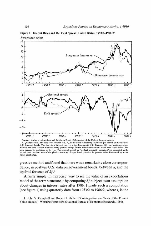
102 Brookings Papers on Economic Activity, 1:1986
Figure 1. Interest Rates and the Yield Spread, United States, 1953:2 1986:2a
Percentage points 16
14 12
10 Long-term interest rate
8 - ..
6
6 ~ ~ ~ ~ ~ ~ ~ ~ ~ ~ *~~~~~Short-term interest rate
2..
0 . 1955:1 1960:1 1965:1 1970:1 1975:1 1980:1 1985:1
4 s , i Rational spread
-2 fuYield spreadshr r
1955:1 1960:1 1965:1 1970:1 1975:1 1980:1 1985:1 Sources: Author's calculations and data from Board of Governors of the Federal Reserve system. a. Quarterly data. The long-term interest rate, Ri, is the yield to maturity in percent per annum on twenty-year
U.S. Treasury bonds. The short-term interest rate, rt, is the three-month U.S. Treasury bill rate, aucom uverage. Ae data are from the first month of every quarter, except for the 1986:2 observation, which used April 4 data. The yield spread, S,, is defined as R, - rt. The rational spread, or "perfect foresight" spread, S,*, is computed as the spread over the short rate of the yield to maturity of a par bond priced at its present value discounted by actual future short rates.
gressive method and found that there was a remarkably close correspon- dence, in postwar U.S. data on government bonds, between S, and the optimal forecast of S,* .
A fairly simple, if imprecise, way to see the value of an expectations model of the term structure is by computing S,* subject to an assumption about changes in interest rates after 1986. I made such a computatio-n (see figure 1) using quarterly data from 1953:2 to 1986:2, where rt is the
1. John Y. Campbell and Robert J. Shiller, "Cointegration and Tests of the Present Value Models," Working Paper 1885 (National Bureau of Economic Research, 1986).
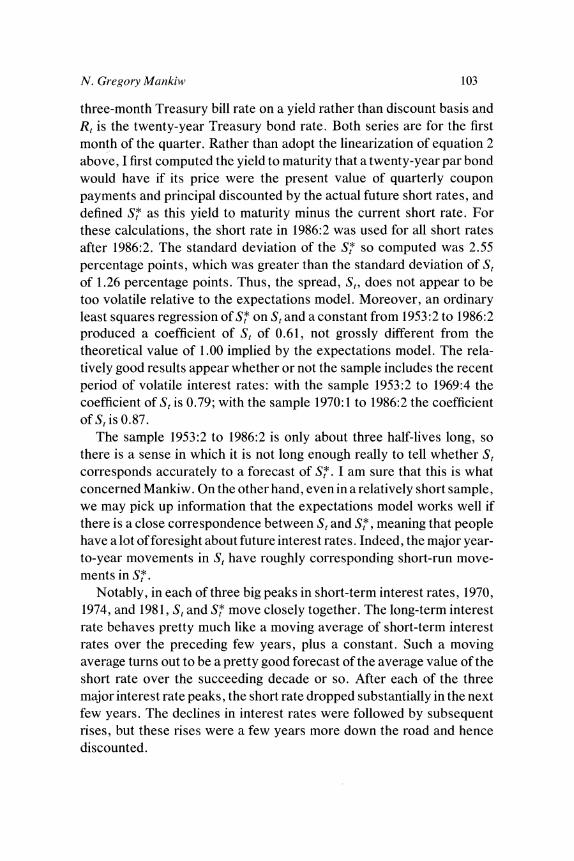
N. Gregory Mankiw 103
three-month Treasury bill rate on a yield rather than discount basis and R, is the twenty-year Treasury bond rate. Both series are for the first month of the quarter. Rather than adopt the linearization of equation 2 above, I first computed the yield to maturity that a twenty-year par bond would have if its price were the present value of quarterly coupon payments and principal discounted by the actual future short rates, and defined S* as this yield to maturity minus the current short rate. For these calculations, the short rate in 1986:2 was used for all short rates after 1986:2. The standard deviation of the S* so computed was 2.55 percentage points, which was greater than the standard deviation of St of 1.26 percentage points. Thus, the spread, St, does not appear to be too volatile relative to the expectations model. Moreover, an ordinary least squares regression of S* on St and a constant from 1953:2 to 1986:2 produced a coefficient of St of 0.61, not grossly different from the theoretical value of 1.00 implied by the expectations model. The rela- tively good results appear whether or not the sample includes the recent period of volatile interest rates: with the sample 1953:2 to 1969:4 the coefficient of St is 0.79; with the sample 1970:1 to 1986:2 the coefficient of St is 0.87.
The sample 1953:2 to 1986:2 is only about three half-lives long, so there is a sense in which it is not long enough really to tell whether St corresponds accurately to a forecast of S*. I am sure that this is what concerned Mankiw. On the other hand, even in a relatively short sample, we may pick up information that the expectations model works well if there is a close correspondence between St and S*, meaning that people have a lot of foresight about future interest rates. Indeed, the major year- to-year movements in St have roughly corresponding short-run move- ments in St*.
Notably, in each of three big peaks in short-term interest rates, 1970, 1974, and 1981, St and S* move closely together. The long-term interest rate behaves pretty much like a moving average of short-term interest rates over the preceding few years, plus a constant. Such a moving average turns out to be a pretty good forecast of the average value of the short rate over the succeeding decade or so. After each of the three major interest rate peaks, the short rate dropped substantially in the next few years. The declines in interest rates were followed by subsequent rises, but these rises were a few years more down the road and hence discounted.

104 Brookings Papers on Economic Activity, 1:1986
Why, if S, behaves so well with regard to S,*, does a regression of excess holding return on the spread (Mankiw's table 7) give such a large and significant coefficient? Mankiw concludes that variables plausibly related to time-varying risk premiums will not provide the answer, and he raises the possibility of measurement error. He shows in appendix B that a small (relative to the variability of the spread itself) serially uncorrelated measurement error that is also uncorrelated with the actual interest rates might account for the large coefficient in table 7. He notes that a serially uncorrelated measurement error with a standard deviation of only 30 basis points could account for a slope coefficient of 2.00. For his results with the U.S. data, where the estimated coefficient was almost 5, the standard deviation of the measurement error would have to be about 40 basis points. Since 30 or 40 basis points represent small errors relative to the standard deviation of St itself, which is nearly 150 basis points, such a measurement error would have little effect on the regres- sions of S* on St. Such measurement error might then reconcile the favorable results in the prediction of S,* by St with the unfavorable results in table 7. But Mankiw doubts that measurement error could be so large.
Since measurement errors are indeed unlikely to be so large, it is natural to wonder whether the same model might hold if the same error term, E, has another interpretation. One appealing interpretation of Mankiw' s results is that E is not measurement error but some proxy for exogenous time-varying risk premiums or for changing attitudes or fashions in investing.
However, not just any scenario along these lines can be reconciled with these data.
Mankiw does not note how large the standard deviation of Ht - rt would be if there were a 30 basis point serially uncorrelated measurement error on the long rate. With p = 0.015 and the standard deviation of E equal to 30, the standard deviation of [(1 + p)Et - et+ J/P on an annual basis would be 28 percentage points, considerably more than the actual standard deviation of Ht - rt (as reported in Mankiw's table 3) of 21 percentage points. Note also that, as he reports in table 3, the standard deviation of the actual quarter-to-quarter change in the long rate for the United States is 48 basis points. If there were a serially uncorrelated measurement error of 40 basis points, then this measurement error would contribute 40 times V2, or 57 basis points, more than the total standard deviation of the change.
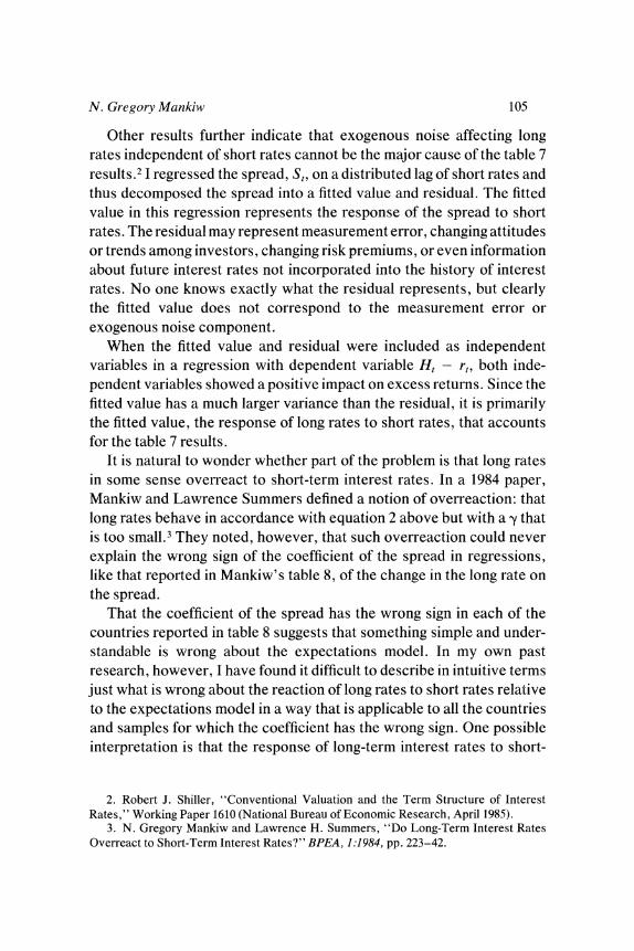
N. Gregory Mankiw 105
Other results further indicate that exogenous noise affecting long rates independent of short rates cannot be the major cause of the table 7 results.2 I regressed the spread, S, on a distributed lag of short rates and thus decomposed the spread into a fitted value and residual. The fitted value in this regression represents the response of the spread to short rates. The residual may represent measurement error, changing attitudes or trends among investors, changing risk premiums, or even information about future interest rates not incorporated into the history of interest rates. No one knows exactly what the residual represents, but clearly the fitted value does not correspond to the measurement error or exogenous noise component.
When the fitted value and residual were included as independent variables in a regression with dependent variable H, - r, both inde- pendent variables showed a positive impact on excess returns. Since the fitted value has a much larger variance than the residual, it is primarily the fitted value, the response of long rates to short rates, that accounts for the table 7 results.
It is natural to wonder whether part of the problem is that long rates in some sense overreact to short-term interest rates. In a 1984 paper, Mankiw and Lawrence Summers defined a notion of overreaction: that long rates behave in accordance with equation 2 above but with a y that is too small.3 They noted, however, that such overreaction could never explain the wrong sign of the coefficient of the spread in regressions, like that reported in Mankiw's table 8, of the change in the long rate on the spread.
That the coefficient of the spread has the wrong sign in each of the countries reported in table 8 suggests that something simple and under- standable is wrong about the expectations model. In my own past research, however, I have found it difficult to describe in intuitive terms just what is wrong about the reaction of long rates to short rates relative to the expectations model in a way that is applicable to all the countries and samples for which the coefficient has the wrong sign. One possible interpretation is that the response of long-term interest rates to short-
2. Robert J. Shiller, "Conventional Valuation and the Term Structure of Interest Rates," Working Paper 1610 (National Bureau of Economic Research, April 1985).
3. N. Gregory Mankiw and Lawrence H. Summers, "Do Long-Term Interest Rates Overreact to Short-Term Interest Rates?" BPEA, 1:1984, pp. 223-42.
106 Brookings Papers on Economic Activity, 1:1986
term interest rates is too smooth.4 A distributed lag regression of long rates on short rates tends to produce a pattern of lag weights that looks too much like a simple exponential decay curve. The exponential decay pattern for distributed lag coefficients seems to apply to a number of sample periods. There should instead generally be a "notch" in the distributed lag at one lag, because of an extrapolative component to short-term interest rates.
With the data in figure 1, a regression of the change in long rates, R, I - Rt, on the spread, S, produces much the same results as Mankiw reports in his table 8: a slope coefficient of - 0. 10, which is significant at the 0.01 level. If long rates are instead R,'- R, + 0.3(rt -. rt ) so that the distributed lag response of the long rate, Rt', to short rates has a notch at one lag, then the coefficient in a regression of R?, 1(1) - Rt' on the spread St'-Rt' - r, produces a slope coefficient that is nearly zero. Still, the spread, St', is hardly any different from the spread we observe: the correlation between St' and St is 0.97.
It seems, therefore, as if people use casual memory or rule of thumb to judge what to expect of interest rates and thus do not properly distinguish sharply between the once-lagged interest rate and the current or twice-lagged interest rate. Putting it another way, while their expec- tations are not far off the mark, there may be a tendency to price long- term bonds with a simple conventional valuation rule.
This may be the main reason for the wrong sign in the table 8 regressions. A less important reason appears to be the above-noted independent noise in long-term interest rates. It is possible to describe a scenario in which the error term, t, had a standard deviation of 50 basis points and a (quarterly) autocorrelation coefficient of 0.9. Then by Mankiw's equation B3 the error term alone would tend to make i equal to something like 0.85 for the countries studied. Such an error term would also be consistent with the results of the instrumental variables regression in table B-1. The standard deviation of [(1 + p)Et - Et]/p
would be 15 percentage points, so that the error term, E, would account for most of the volatility of quarterly holding period returns. By this measure, long-term interest rates would show substantial excess vola- tility relative to the expectations model, and yet the excess volatility
4. Shiller, "Conventional Valuation and the Term Structure of Interest Rates."
N. Gregoty Mankiw 107
would be only a minor contributing factor to the rejection of the expectations model in table 8.
In light of this scenario, how can we explain the recent dramatic drop in the long-term interest rate, Rt? In the data plotted in figure 1, the decline from October 1985 to April 1986 was 2.79 percentage points, a drop rivaled only by the 2.98 percentage point drop between July 1982 and January 1983. The latest decline is certainly unique in that it occurred when the short rate, rt (figure 1), fell only 0.99 percentage point over the two quarters, in contrast to 4.31 percentage points between July 1982 and January 1983.
We thus have in the latest drop in long rates a drop in the spread that is not explained by an increase in short rates, as is usual.
The latest decline in the spread might be attributed to a sharp decline in the noise term, E, let us say an exogenous change in investor attitudes.
By the parameter values in the scenario described above, the decline in E would have to be unusually large by historical standards. However, we should not apply historical standards to Et at a time when time series properties of interest rates are clearly changing. The recent volatility of interest rates and unusual concern with government deficits may well have increased the variance of E. Psychologists have shown that the variability of attitude change is not constant but is heavily influenced by salient events. The expectations theory of the term structure is no reason not to ascribe most of the recent drop in the spread to capricious public attitude change.
General Discussion
Albert Wojnilower suggested that the relative supplies of new secu- rities of differing maturities ought to be more integrally incorporated into studies of the interest rate term structure. A major objective in the borrowing decisions of the Treasury, the largest issuer of securities in the U.S. market, is to keep the average maturity of the debt approxi- mately constant, with little if any attention paid to the relative cost of borrowing at different maturities. James Tobin interjected that the Treasury has indeed made peculiar choices regarding maturities, in recent years issuing long-term securities at market rates exceeding their own predictions by several hundred basis points. If the Treasury pays
108 Brookings Papers on Economic Activity, 1:1986
no attention to the costs of borrowing at different maturities, Wojnilower continued, it may be unrealistic to expect the purchasers of Treasury securities to perfectly arbitrage expected returns. Mankiw responded that previous work has found relative interest rates to be insensitive to relative asset supplies. Moreover, relative supplies of securities of different maturities change slowly, so that shifts in relative supplies cannot explain short-run variation in the term structure.
William Poole recommended comparing securities of constant dura- tion rather than those of constant maturity. The maturity of a portfolio equals the weighted average of the time remaining until the principal is due, with the weight for each bond equal to the nominal dollar value of the principal. The average duration of a portfolio equals the weighted average of the time remaining until future coupon and principal payments are due, with the weights reflecting the present value of the payments to be made at each date. Hence, duration is responsive to the level of the interest rate. Average duration shrinks when the interest rate rises because more of the present value of the stream of payments associated with a bond becomes concentrated in the first few years.
A number of participants wondered how changes in the institutional environment over time might have affected the structure of interest rates. George Perry was especially interested in the figure in Robert Shiller's discussion. Assuming that investors have accurately forecast changes in the short-term interest rate, he noted, the bottom panel of the figure implies a relatively stable long-term bond premium of about 200 basis points from the early 1950s through 1970, roughly equal returns on long-term and short-term securities during the 1970s, and a premium for holding short-term securities of about 400 basis points during the first half of the 1980s. Neither Mankiw nor his discussants offered any explanation for these long-term shifts in their formal presentations. However, Mankiw noted that the premium for holding long-term rather than short-term securities cannot necessarily be inferred from Shiller's plot; the expectational errors implicit in this plot tend to be serially correlated, so that one big surprise could create the persistent divergence in the figure.
Several participants discussed possible determinants of the term structure that were not included in Mankiw's analysis. Wojnilower mentioned recent institutional changes: the move from fixed to flexible exchange rates; changes in the debt management policy of the Treasury;

N. Gregorv Mankiw 109
new financial regulations; and interest rate controls. He also reasoned that changes in the monetary policy regime such as the one that occurred in October 1979 might have affected expectations of the possible paths of future short-term rates. Mankiw responded that the estimated rela- tionships among interest rates looked very similar across subperiods, including the subperiods before and after flexible exchange rates and those before and after the Federal Reserve's 1979 shift in emphasis from interest rates to monetary aggregates. While further investigation might unearth something interesting, he acknowledged, preliminary explora- tions did not look promising.
Tobin added that the term structure could at times reflect different expectations of buyers and sellers, in contrast to the usual rational expectations assumption that all participants use the same information and model of the economy. For example, during the depression, Keynes had conjectured that lenders expected interest rates to rise toward their historical average, while borrowers did not foresee the economic events that would justify such a rise. During the 1970s and early 1980s, lenders may have been so conditioned by a long period of capital losses in bonds that they feared still higher bond prices, while borrowers did not foresee economic events that would justify such high long-term rates. Tobin added that preferred habitats of borrowers and lenders with respect to the maturity of debt might differ for other reasons as well and that these differences might vary through time, contributing to the observed variation in the term structure.
William Branson noted that securities markets were linked interna- tionally and that investors chose not just between long- and short-term rates within one country, but between rates in different countries. An analysis that exploited data from several countries more fully would have to consider the relations among interest rates in different countries, along with the exchange rates linking them.
Tobin noted that the equations in table 7 implied quite different term premiums across countries, with the expected steady-state return from holding a long bond rather than a series of short securities ranging from 114 basis points to 350 basis points. One might well ask why there should be a term premium at all if rates are not changing; in effect, the table 7 equations simply reproduce the average spread between long rates and short rates for the period over which they are estimated, without revealing the underlying reasons for the spread. Beyond the question of

110 Brookings Papers on Economic Activity, 1:1986
why there should be any spread, there is the question of why it should be so different across countries. George von Furstenberg suggested that one explanation might be international differences in tax codes. For example, in Germany capital gains on bonds held six months or longer are tax free, whereas in the United States such gains are taxed at 40 percent of the rate applicable to earned income. Offsetting this, German banks receive a credit against non-interest-bearing reserves equal to 10 percent of their holdings of short-term government securities. This would imply that short-term interest rates should be 10 percent lower than otherwise relative to long-term rates. Wojnilower noted that the yield curves for corporate securities and for municipal bonds are quite different; a careful examination of the differences between these two markets might yield useful insights concerning determinants of the term structure.
Von Furstenberg questioned the comparability of the German data with that for other countries. Until recently, the German government issued no short-term securities and very few long-term securities. The three-month interest rate for Germany is of necessity a commercial paper rate, while that for the other three countries compared by Mankiw is a government security rate. Market quotations for the German long- term government bond rate were not available until the 1970s. It is noteworthy that the three-month Treasury bill rate averages 100 to 150 basis points below the three-month Eurodollar rate, while the German three-month rate used by Mankiw averages above the three-month Euromark rate. This makes it doubtful that Mankiw's series on long- and short-term German rates can be compared in a term structure equation. It also makes cross-country comparisons of the term structure equations suspect.