THE THEORY AND APPLICATION INEAR OPTIMAL … · THE THEORY AND APPLICATION OF LINEAR ... Mr. W. Shed and Mr. C. Mesiah for computing services and Mrs. J. Martino ... a scalar expression

f

This Docunlent

AFFDL-TR-65-28 l4PFroduced FromnBesttAvailable Copy

THE THEORY AND APPLICATION OF

INEAR OPTIMAL CONTROL

S~~~~EDMU'ND G;. IRYA.SKI A.N'D I3ICIIAW) V. W11171 E.CK

CORNELL ,,i'RON.\>A TIC.I. LA( )t..\ TORY, INC(.

TECIINICA\ IR.EPOR)T AFFI)I ,-II-fi5-28

C L. A pl I N f2 0 U S EFOTF•T.' ~i.ir1 -1-0 ANID

_,'- J..\NUAIY 1966

;UZ' Ut '

SDistribution of This Document Is UnlimitedI

AIR FORCE FLIGHT DYNAMICS LABORATORYRESEARCH AND TECHNOLOGY I)IVISION

AIR FORCE SYSTEMS COMMANDWRIGHT-PATTERSON AIR FORCE BASE, OHIO

NOTICES

When %overnment drawings, specifications, or other data are used for anypurpose other than in connection with a definitely related Government procure-ment operation, the United States Government thereby incurs no responsibilitynor any obligation whatsoever; and the fact that the Government may haveformulated, furnished, or in any way supplied the said drawings, specifications,or other data, is not to be regarded by implication or otherwise as in anymanner licensing the holder or any other person or corporation, or conveyingany rights or permission to manufacture, use, or sell any patented inventionthat may in any way be related thereto.

Copies of this report should not be returned to the Aeronautical SystemsDivision unless return is required by security considerations, contractualobligations, or notice on a specific document.

600 - February 1966 - 773-32-683

- ,,�.,', V.

t .

ii

.4.

BLANK PAGE

I V

4

.1

/ I.>7.; A �rw'-'��"---- - ... Ia L.tI

AFFDL-TR-65-28

THE THEORY AND APPLICATION OFLINEAR OPTIMAL CONTROL

EDMUND G. RYNASKI AND RICHARD F. WHITBECK

Jo sI

IfI

/'D stributdon of This Document I. Unlimited

FOREWORD

The research documented in this report was performed for the AirForce Flight Dynamics Laboratory of the Research and Technology Division,Wright-Patterson Air Force Base, Ohio. by the Flight Research Departmentof the Cornell Aeronautical Laboratory, Inc.. of Buffalo. New Ynrk. Thismiucy was Gone under Air Force Contract No. AF33(615)-1541, Project No.8219 'Stability and Control Investigation". and Task No. 821904. The pro-ject ---. administred- by Mr. Frank George oi the Flight Dynamics Labora-tory. The work was performed primarily by the principal investigator,Mr. Edmund Rynaski, and by Dr. Richard Whitbeck.

Important suggestions and guidance were provided by Mr. R. Andersonof the Flight Dynamics Laboratory, and by Mr. W. Deazley, Mr. J. N. Ball,and Mr. J. M. Schuler of Cornell. Grateful acknowledgement is made toMr. W. Shed and Mr. C. Mesiah for computing services and Mrs. J. Martinoand Miss D. Kantoreki for their report preparation skills. The researchdocumented in this report is based upon the original theories developed byDr. R.E. Kalman and Dr. S.S.L. Chang.

This report is being published simultaneously as Cornell AeronauticalLaboratory Report No. IH-1943-F-I.

Manuscript released by authors October 1965 for publication as anAFFDL Technical Report.

This technical report has been reviewed and is approved.

C. D. M rTBDO*Mlt# Co•nwl C1te1a DimbAF PUght ftneos Laboeatory

-I- m m m m m m m m m m m m m m m I

.4-

ABSTRACT

Linear optimal control theory has produced an important synthesistechnique for the design of linear multivariabla systems. In the presentstudy, efficient design procedures, based on the general optimal theory.have been developed. These procedures make use of design techniques whichare similar to the conventional methods of control system analysis. Specifi-cally, a scalar expression is developed which relates the closed-loop polesof the multi-controller, multi-output optimal system to the weighting param-eters of a quadratic performance index. Methods asalogous to the root locusand Bode plot techniques are then developed for the systematic analysis ofthis expression. Examples using the aircraft longitudinal equations of motionto represent the object to be controlled are presented to illustrate design pro-cedures which can Us carried out in either the .ime or frequency domain*.Both the model-4n-the-performance-index and model-following concepts areemployed in several of the examples to illustrate the model approach tooptimal design.

iii

TABLE OF CONTENTS

Section Page

I INTRODUCTION ...... .. . ..... . 1Background. .. 2 . . . .Reader's Guide . . . . . . . . . . 5

2 SURVEY OF LINEAR OPTIMAL SOLUTIONTECHNIQUES . . . . . . . . . . . . . . . 7

2.1 Introduction. . . . . . . . . . . . . . 7

2.2 The Method Attributable to R.E. Kalman (Reference 1) . 7

2. 3 The Method of Merriam (Reference 5) . . . . . . . 9

2.4 Pontryagin's Technique (Reference 4) . . . . . . . 11

2.5 The Method of Chang (Reference 3) .... • . . . 13

2.6 Direct Solution. 16

3 THE ROOT SQUARE LOCUS . . . . . . . . . 20

3.1 The General Problem * . * . . ....... 20

3.2 The Root Square Locus Derivation . . . . . . .. 21

3.3 Numerical Example -Root Square Locus. .. . . . 31

3.4 Root Square Locus - Control Rate in thePerformance Index . . . 36

3.5 Root Square Locus - Output Rates'in thePerformance Index ............ , 39

3.6 Root Square Locus - Model in thePerformance Index . . . . . a .0. . . . . . 41

3.7 Model and Plant Exactly Matchable . . . . . . . . 44.

4 THE SINGLE CONTROLLER LINEAR OPTIMAL SYSTEM 574,1 Introduction. . , . . . . . . . . . . . . . 57

4,2 Feedback Gains as a Function of Q and R. . . . . . 57

4.3 Performance Index for Restricted Feedback ..... 60

5 LONGITUDINAL SHORT PERIOD OPTIMAL

FLIGHT CONTROL . . . . ......... 64

5.1 Introduction. . . . . . . • . . . . • , 64

5.2 A Design Philosophy . .. . . . . . . . . . 64

5.3 Numerical Example of Analysis Over a Flight Range . . 68

iv

TABLE OF CONTENTS

(CONTINUED)

Section Page

6 MINIMIZATION IN THE FREQUENCY DOMAIN -rT'U QWI- ~TtT W i A 13T A nT W rnirf~U T Lif 9L

6.1 Introduction . . . . .. .... ... 76

6.2 Theory for the Optimum Transfer Function # . • • 76

6.3 The Optimum Control . .. .. . . ..... 81

6.4 Examples . . .a o * a o @ a . 83

6.5 The Problem of a Type Zero Plant . . .... . . 86

6.6 Problem of Obtaining a "Good" Low Frequency ResponseWhen no Free Integrator Appears ..... . a • * a 87

6.7 The Problem of the Free Integrator UsingS.S.L. Chang's Approach . . . . . . . .. . . 88

6.8 Equivalence Between the Time Domain State VectorApproach and the Frequency Domain Approach ... 90

7 MINIMIZATION IN THE FREQUENCY DOMAIN -THE MULTIVARIABLE PROBLEM. . . . .0. . . 98

7.1 Introduction. . . .. .. .. .. . . . . 98

7.2 The Regulator Problem. . . . o . . a . # . . 98

7. 3 Factorization of the Matrix . . . . . . . . . o 101

7.4 Direct Formulation in the Frequency Domainin Terms of Transfer Functions . ... . . . L . 105

7.5 Factorlzation Example . . . . . . . . . . . . 105

7.6 A Direct Solution of the Optimal Control Law . . . . 1087.7 Model Following. . . . . . ....... 114

8 USE OF BODE PLOTS IN LINEAR OPTIMAL DESIGN. . 124

8.1 Introduction. . . . . . . . .. . . . . . . . 124

8.2 Single Variable Case* .. . , . .e • a • • • 124

8.3 Extension to Multivariable Case . . . . . . . . . 126

8.4 Steps in a Frequency Domain Design Procedure. . . . 130

8.5 Design Problem with Bode Plots. . . . . . . . . 130

9 A MULTIVARIABLE EXAMPLE. . . . . . . . . 145

9.1 Equations of Motion . ........... 145,

9.2 Model in the Performance Index. . . . . . • 147,

9.3 A Complex Model-Following Design Problem . . • . 158

9.4 An Alternate Design Philosophy for Model Following . . 178

V

I TABLE OF CONTENTS(CONCLUDED)

1j 16 CON5CLUSIONS . 180

U.EU'KENCES * . * * . * ** . . . . . 182

APPEHIWMI - DE VE LPMIENT OF H [is - F-1 P- S A M A MnT%1

OF TRUMP=FUFUNCTIONS. . ...... 8

SPPZEM U - DE VELOPMENT OF G'[-Is - F'J H'QHfIs - 01

vi

T TC'rI eC% C11111ItrAm

Figure Page

I Single Output Block Diagram . . ........ 13

2 Alternate Block Diagram ........... . is

3 Root Square Locus Plot - Single Input Example . . . 34

4 Flow Diagram of Optimal Regulator. . . . . . . . 35

5 Root Square Locue - Model in the PerVforrmaivce Iin. 0 49

6 Locus of the Roots of the Optimal System Model in thePerformance Index . . . . . . . a . .. a . 55

7 Locus of the Roots of the Optimal System -Position Feedback Only*. . . .... .. &1

8 Locus ofZeros of (,)kt () . ..... . .*

9 Sketch of the Poles of the Optimal System forSeveral Values of k . . . . * 0 . * . . a .. . 67

10 Root Square Locus for the Performance Criterion

2V' ;•f((h:.3AX,)q#PrAS4]d$ - Power Approach. . * 73II Root Square Locus for the Performance Criterion

2V. 1fe ,.3s r, r'• 9]dt - Mach= 0. 5. h = Sea Lem] 7312 Root Square Locus for the Performance Criteriom

2V., ((5k #, RA id t 1 Mach z 0. 9. h = Sea Leval 74

13 Root Square Locus for the Performance Criterion2V g " ((d ~ ##o4&.,M~k0- Mach = l+, h =Sea Level, 7

S014 Root Square Locus for the Performance Criterion

2V" PA •••'Ae dldt"- Mach = 0. 6. h :w 40. O00 ft.: 75

15 Root Square Locus for the Performance Criterion

2V [(Avf#(-.J~wpi"qe rA&sJ81d Mach = 2+, h =60P 06W ft 7516 Single Control Optimal System ........ . 7617 Single Control - Single Output Optimal System . . * Si18 Single Output Optimal System . . . .... . s8

19 Block Diagram of /•U .. .. .... 91

20 Feedback Configuration. . ...... . . .# 93

21 Closed-Loop Configuration. . . . . . .*. . . 96

22 Alternate Feedback Configuration . . . . . . . . 97

23 Block Diagram of System with Two Controls andaSingle Output* . . o . • . . • . . . 106

24 Open-Loop Plant . . ..... .. .11. 1725 A Specific Feedback Configuration . . . . .. . 121

vii

5~W . -7-- __ _

LIST OF FIGURES(CONTINUED)

26 Single-Input, Single-Output Model-Following System . . 121

27 First Unity Feedback Form . .. ..... 125

28 Second Unity Feedback Form . . . . ...... 125

29 Expanded Plot of the "0* Line" on a Nichols Chart. . . 127

30 First Feedback Form for Multivariable System. . . . 129

31 Second Feedback Form for Multivariable System . . . 12932 Block Diagram of Open-Loop System . . . . . . . 131

33 Unity Feedback Form for Design Problem ..... 13.2

34 Bode Plot of First Stage, 9,,q = 2.4. .4. . . . . 135

35 Bode Plot of First Stage, .,/q, Variable . . . .. 136

36 Closed-Loop Poles asa Function of q9/r . . . .. 138

37 Closed-Loop Roots with q/"/r as a Parameter . . . . 141

38 Closed-Loop Roots for 9, i q5 as a Function of I.,/r . 144

39 Realizable Part of the Model-in-the-PerforrrAnce-IndexRootSquare Locus . . . . . . .... . . . 157

40 Unity Feedback Block Diagram for FindingClosed-Loop Poles ............. 165

41 Ulf //, 9 , q/ as the Parameter. . . . 168

42 idru/e,/4 "3/1•1 as the Parameter ........ 168

43 •/ut ,'q2 /r as the Parameter ....... 169

44 elf , as the Parameter .... 169

45 9/q, Versus r,-/r, . . . . . . . . . . . . 17046 Block Diagram for Approximate Expression . . . . . 17147 l/rn , •'Z/•, as the Parameter . .. .. .. 172

48 Block Diagram Describing Approximate Root Square Locus 173

49 1,ll, r ,f•lr, / 1 //OO . . . . . .... . . . 17450 ,rfal 1,, . . . . . . . . z7451 Plant and Model Root Locations in the Complex Plane. . 175

52 6V Response of Model and Plant . . . . .... 177

F 53 Ao Response of Model and Plant. . . . . . . . 177

"54 Plant and Model Roots for Alternate Design Philosophy . 179

I-I Flow Diagram of Two-Input, Two-Output System . . . 186

S~viii

LIST OF TABLES

Table Page

1 AERODYNAMIC DERIVATIVES . . . . . . . . 68

2 TRANSFER FUNCTION PARAMETERS . . . . .. 69

3 AERODYNAMIC DERIVATIVES . . . . . . . . . 146,

4 GAINS SYNTHESIZED FROM DESIGN PROCEDURE . . 176

ix

72'

LIST OF SYMBOLS

Vmi~ni- £

state vector; whose components define the variables of thefirst-order set of equations of motion of the plant

the output vector; defined by a transformation on t , theset appearing in the performance index

a the control vector; the input to the plant

the optimal control vector; the input motion that forces theplant to respond optimally

the adjoint state vector; the undetermined multiplier of theEuler- Lagrange equations

%(s) the Laplace transformed state vector

y(s) the Laplace transformed output vector

a,(s) the Laplace transformed control vector

•g,(s) the Laplace transformed optimal control vector

Zt(s) the Laplace transformed adjoint state vector

generalized deterministic disturbance vector

a(s) the Laplace transformed disturbance vector

vector defined to be analytic in the left-half plane

model state variable

fictitious state vector associated with the model in theperformance index; # =/"

(s) a vector consisting of polynomial entries which define thenumerators of the optimal control

Matr ice s

P" n x n matrix; matrix of constants that define the interactionsamong the state variables of the plant

Q n x p input matrix; matrix of constants defining the effectof a control on the state rates

/1r x n matrix transformation on x that define a the output,y = Hx

x

Matrices (continued)

Q r x r matrix of constants that weight the output in theperformance index

p x p matrix of constants weighting the control in theperformance index

L. the model system inatrix; matrix of constants definingthe interactions among the model state variables

matrix of constants weighting the output rates in theperformance index

Smatrix of numbers weighting the derivative of the statein the performance index

T matrix of constants weighting the control rates in theperformance index; collinear transformation % ut

to transform the state vector to a set of uncoupled equations

Svariable of the Riccati equation

matrix of feedback gains, Id R-'fQ P

identity matrix

A. modal matrix

[Is-F•' transition matrix of the plant

(s = W(s) = matrix of transfer functions relating the outputsy. (s) to the inputs uj (s)

W$) = H Is- F] = transition matrix of the output

Matrix and Vector Notation and Abbreviations

[ ] denotes a matrix or a vector

I i denotes a determinant

LI transpose of a vector or a matrix

[ ]' inverse of a matrix

[I"' adjugate of a matrix defined by ] [AA]"'/A1

] conjugate of a polynomial matrix of s, W(-s) = W(s)

[ ], conjugate transpose of a polynomial matrix of a,

xi

,lit4

I Matrix and Vector Notation and Abbreviations (Continued). .i ..

- "& . .... -,aa.roLn5 in the is-' row and J1" column

j (~O) initial conditions of a vector

[ ]i the ith component of a vector

lhp left-hand planerhp right-half planemin minimumlir limitsup supremum - least upper bound

or. optimumd~n dimension

Determinants and Scalars

D(s) characteristic polynomial of the open-loop plant, D(s) I I s-F1

1(S) characteristic polynomial of the optimal system, d(v)vjIs.FkI

Atj firstminor obtained'by deleting the ith row and jth columnof JIB - Fl

5() :s = (-s)

Aq kid second minoI obtained by deleting the ith and kth rows andthe jth and Itn columns of IIs - FI

$= 0d j&) , Laplace transform variable

V/ the performance index, 2V

the integrand of the performance index, 7 1 ' (YIQY #URa')r(s) left-half plane poles of W5•8(Ob*a(s)D)excluding

the open-loop poles, D(s)

the Lagrangian function; ekf = * 1'. (- 0 ) Pi+.

the Hamiltonian function, 2=e - * ,.;V (F'i %,&)

Aircraft Notation

incremental pitching velocity, deg/sec

A 0 incremental pitch angle, deg

b OC incremental angle of attack, dog

16V incremental change in airspeed* ft/eec

xii

a Min-.

Aircraft Notation (Continued)

-A- S

incremental change in thrust, lb'

CO short period natural frequency, rad/sec

short period damping ratio

cot phugoid natural frequency, rad/sec

phugoid damping ratio

i

0,

xill

!I

SECTION 1

INTRODUCTION

AI his report cescribes the results of a study of the characteristics of!•linear optimal control. As used in this report. a system describable by a metL c••.•••o n s t nt" coe= fftc tnt lirear differen~tial equation~syseof motionsyteis saidby ...to~ |belin-

ear, Optimal control is a technique for control system synthesis by which**'iunique control input motions are specified that minimize a functionaleromac of the ms-Stions'of the system. This functional is called a efrac index. Linear

"'optimal control is an optimal control synthesis procedure for linear systorn,whereby the control motions are uniquely determined by a feedback law con-

'sisting of a constant linear sum of the variables, or states of the system.

Mathematically, the problem can be defined as follows:

* • For some initial condition of the state, • (0), find the control •, thatmninimizes the quadratic performance index

2V- We* 'Q)dt

"subject to the natural constraint of the linear, constant coefficient equations ofmotion of the plant written in the first-order form

The performance index is a scalar quantity consisting of an infinite in-tegral of sums of quadratic functions of the outputs and the control inputs to

, the system. Using linear optimal control, this index supersedes all conven-tional performance criteria such as rise time, overshoot, damping ratio, etc.It becomes necessary then, to express control system performance in termsSof the elements within the performance index. In order to select this perform-ance index properly, it is important to be able to predict the closed-loop char-acteristics of the system in terms of conventional performance criteria. Iflinear optimal control can satisfy most conventional criteria, it will be a use-ful tool for linear system design. If it inherently provides additional advan-tages, then linear optimal control becomes an important tool in the design oflinear control systemo,.

In this report, the relationships between conventional design criteriaand optimal design criteria are investigated to determine whether or not op-timal control can satisfy conventional design criteria; it can. In addition,other aspects of optimal control are investigated to determine if additional ad-vantages exist by designing a system using linear optimal control. They doexist. Seldom, if ever, does a relatively new technique produce design ad-vantages without limitations and disadvantages. Linear optimal control is re-stricted in its usage and does possess disadvantages if not properly used.

"4 •Linear optimal control is a general multivariable systhesis technique.Multi-controller, multi-output systems of high order can be conceptuallydesigned very quickly using a digital computer and a unique control systemwill be specified for any one performance index. Using conventional techniquesand criteria, a multi-controller design can be a tedious chore. Frequently,

ii~i -

the resulting system configuration will not be unique.

The use of linear optimal control techniques guarantees that the re-sulting closed-loan avnkt~w will ha -ahlkl. Th' ,.C•.,•J- "..4- . k..L* .S ,I .

plex frequency plane is eliminated as an area where closed-loop roots mayexist. This feature of the technique can be important when the vehicle to becontrolled is inherently unstable or flexible. The difficulty is that it may notalways be possible to physically mechanize a system designed to stabilize anunstable vehicle or to minimize bending mode flexibility.

The closed-loop transient response of a linear optimal system tends tobe smooth and well behaved. As the output is weighted heavily with respect tothe control, the closed-loop response closely resembles the response of aButterworth filter, whose transient response has little overshoot ( r = . 707for a second-order system) and whose frequency response is flat. Frequently,a linear optimal system has dynamic characteristics that an engineer strivesfor when using trial-and-error, conventional control system design procedures.Using optimal techniques, the controller motions can be qualitatively controlled.If a particular optimal design requires control input amplitudes larger than isdesired, it is necessary only to increase the weighting of the control portionwithin the performance index, penalizing control motions more heavily. In thisway, the control amplitudes may be reduced with, of course, an accompanyingdecrease in the speed of response of the closed-loop system.

The primary limitations of linear optimal control lie with the selectionand interpretation of the performance index and the possible difficulty in phy-sically mechanizing the resulting optimal control law. It appears easiest toselect a performance index for the design of a completely automatic regulatingsystem. For instance, it is not difficult to conceive of a performance index tosatisfy many of the requirements of an automatic mid-air refueling system.In this application it is possible to identify dynamic variables that must be min-imized, such as relative position errors between the two aircraft and the bend-ing moments of the refueling aircraft. On the other hand, it is not knownwhether a quadratic performance index ban be selected for the design of sta-bility augmentation systems. Acceptable flying qualities are defined in termsof conventional dynamic criteria, such as short period natural frequency,damping ratio and lift curve slopes, and these quantities must be related tolinear optimal design criteria before definite judgments can be made. How-ever, because of the smoothness and generally well behaved dynamic charac-teristics of linear optimal systems, there is reason to believe that systemsdesigned by linear optimal techniques will be judged acceptable for manualoperations.

BACKGROUND

The solution to the linear optimal control problem probably evolvedfrom the calculus of variations but its significar -e was not fully appreciateduntil R. E. Bellman and L. S. Pontryagin rigidly stated the conditions underwhich an optimum exists. The complete solution in the time domain was re-cently obtained by at least two prominent control system theorists, R. E. Kal-man (Reference 1) and C.W. Merriam III (Reference 5). Kalman and Merriamhave not only rigorously obtained mathematical proofs of the solution and

1

related theoretical aspects of the problem, but have been instrumental in de-veloping digital computer programs for machine solution of large multi-controller oroblems. in th. fr.qiny Anmnin. *I%^ ,n.i__ina • s 1.t_ -.,h W-.

was extended by Mssrs. G. Newton, L. Gould and J. Kaiser. The problemwith quadratic control constraint was solved completely in the scalar case byS. S. L. Chang (Reference 3).

Under Air Force Contract AF33(657)-7498, the Flight Research Depart-ment of the Cornell Aeronautical Laboratory investigated the application oflinear optimal control techniques to several control system problems associ-ated with aerospace vehicles using the digital computer program developed byT.S. Englar and R.E. Kalman (Reference 2).

It was found that the design technique has definite merit. Stable, well-behaved closed-loop systems can be conceptually specified using linear optimalcontrol techniques. Large multivariable systems can be easily handled andmany closed-loop optimal systems can be computed in a relatively short per-iod of time. It was also discovered that, with practice, the control systemdesigner could often qualitatively relate the parameters of the performanceindex to those dynamic characteristics known to yield an acceptable flight con-trol system.

This report describes the results of an intensive study whose objectivewas to obtain relationships among the performance index parameters and theclosed-loop optimal dynamics. The results show that the weighting parametersand the closed-loop poles are directly related. Both time and frequency domainapproaches were used to minimize the integral performance index. The timedomain approach used conventional calculus of variations techniques. The fre-quency domain approach uses Parseval's theorem in the manner advanced byS. S. L. Chang. Equivalence between the two methods can be demonstrated.The time domain approach uses the characteristic equation of the Euler-Lagrange and constraining equations to obtain a root square locus expression.The optimal control is shown to be governed by the matrix Riccati equation.The frequency domain approach shows that the conditions for optimality re-quire the solution of a matrix Wiener-Hopf equation. A determinant can beextracted from the Wiener-Hopf equation that results in a root square locusexpression for the closed-loop poles. The optimal control can be obtained bysolving the Wiener-Hopf equation either by:

I. spectral factoring, or2. a direct solution technique.

Many examples (both single-input and multi-input) are given in this re-port to demonstrate certain characteristic~s of linear optimal control. Exam-ples of the root square locus and the equivalent Bode plots are numerous.Many of the examples use the equations of longitudinal aircraft motion to des-cribe the object to be controlled.

The use of models to obtain a desirable closed-loop optimal system isalso studied in this report. Specifically, the model can be included in the de-sign objectives in two ways: the model can be included in the design as aninput (as an uncontrollable part of the plant) or the model can be mathematicallyincluded in the performance index only. Examples to illustrate model proce-dures are given.

3

A significant start has been made on the problem of determining use -ful relationships between the feedback gains and the performance index. Inthe case of the single controller, the problem has been solved through the useof the root square locus expression as a design aid. :For the single-input,singie-output case, it is shown that a perlormance index can be formulated toyield specific feedback gains, closed-loop frequencies and damping, or spe-cific ateady state -characteristics to a specified input.

The report describes the exact relationships that exisý between theperformance index parameters al&d the closed-loop optimal system poles.Because of this, one of the primary relationships between good aircraft fly-ing qualities and optimal control c haracteristics has been established. How-ever, more research is necessary to describe, in a usable, easily predictableform, the relationships between the optimal control law and the performanceindex.

This report places primary emphasis upon the relationships that existamong the parameters of the performance index and the resulting dynamiccharacteristics of the closed-loop optimal system. It is felt that a basic un-derstanding of these relationships, and the optimal systems that they produce,is a prerequisite to their actual application. Optimal control can be anothervaluable addition to the design tools available to the flight control system de-signer. Some of the pertinent areas of application are emphasized in the ex-amples included in this report. It is felt that this report will contribute to abetter understanding of the technique, and accelerate its application to appro-priate problems of control system design.

In Section 2 the optimal regulator of a second-order single-input,single-output system is obtained using the notation and basic techniques of11. Z. Kalman, C.W. Merriam III, L.S. Pontryagin, S.S.L. Chang and a di-rect solution technique. The object of this section is to show that a unique op-timal regulator is obtained regardless of the technique used. This sectionalso shows that the techniques are basically the same, requiring the solution ofa Riccati equation when formulated in the time domain and a Wiener-Hopfequation when formulated in the frequency domain.

In Section 3 of this report, the root square locus expression is devel-oped. The integral is minimized by satisfying the Euler-Lagrange equations,whose characteristic determinant contains the closed-loop poles of the optimalsystem and adjoint. This characteristic determinant is manipulated into aroot square locus expression. Performance indices containing control rates,output rates and models are considered, and the corresponding root squarelocus expressions are obtained.

Section 4 discusses some of the aspects of the single-input system,and shows that the problem is simply solved. The performance index can berelated to the closed-loop dynamics and the optimal feedback gains. A per-formance index can be formulated to yield a predetermined feedback gain,including no feedback from a state variable, if desired. In general, however,negative values of 91i in the performance index must be allowed.

Section 5 shows how optimal control techniques can be effectively used

4

to specify a control system design for the longitudinal short period control ofa modern, high performance fighter aircraft.

The theory of the optimal control law for a system with a single controlvariable and a single output variable, using the frequency domain technique ofS.S. L. Chang, is considered in Section 6. Several examples are given to il-lustrate the application oi the method and to point out some difficult pointswhich occur in the theory. The equivalence between Chang's method and thetime domain approach is demonstrated.

The frequency domain approach of Section 6 is extended to the multi-variable situation in Section 7. It is shown that the frequency domain relationof interest is a matrix equation of the Wlener-Hopf type. This matrix equttioncan then be solved using either of two methods:

1. spectral factorization, or2. a direct method.

Examples are given to demonstrate the factorization approach and the directmethod.

A subsection is included to show how one arrives at the matrix Wiener-Hopf equation when the basic description of the system is given in terms oftransfer functions rather than a set of first-order differential equations. Thesection concludes with a theoretical development of the model-following tech-nique and a method for synthesizing the feedback gains required by the optimalsolution.

In Section 8, the use of Bode plots in linear optimal design is outlinedin detail. A relatively complicated design problem, involving a jet fighterin a power approach, is used to illustrate the application of the concept. Thesection concludes with the outline of a frequency domain design procedure.

A more complex multivariable example of the use of the root squarelocus and the equivalent Bode plots is given in Section 9. The problems ofdynamically matching a small jet to a proposed supersonic transport are il-lustrated using both the model-in-the-performance-index technique and themodel-following concept.

This report is concerned with the solution of the problem involving aquadratic performance index. This index has shown to yield acceptable de-signs for many applications. One can always speculate on whether or not abetter design would have been obtained if a different performance index hadbeen used as the design criteria. Several excellent reports have been writtendescribing the characteristics of systems designed using other performanceindices (for instance, see References 16 and 17) and solutions to these prob-lems using a suitable and realistic control constraint may eventually lead to avery useful set of design tools for the practicing engineer.

READER'S GUIDE

Most of the comments on the uses and abuses of linear optimal controlare contained within the introduction and conclusions of this report. Thosewho are not mathematically minded, or those busy management people whodecline to become too technically involved are urged to read only the Abstract,

5

Introduction and Conclusions.

Those who are more theoretically inclined would find Sections 3 and 7most challenging. Section 3 contains most of the developments in the time do-main and is the source for the derivation of the multi-output, multi-controllerroot square locus expression. Section 7 derives the frequency domain matrixWiener-Hopf equation and describes a direct method for solving the Wiener-Hopi equation.

The engineer interested in optimal control, but either not familiar withmatrix manipulations or who prefers relatively simple examples, will find thatSections 2, 4 and 6 will provide him with a fair understanding of the relation-ships between conventional and optimal design procedures.

Section 5 illustrates how the root square locus concept might be usedfor flight control system analysis and conceptual design, while Section 8 out-lines the use of Bode plots in linear optimal design.

"Finally, two multi-output, multi-controller examples are presented inSection 9 in connection with the use of models to obtain satisfactory and ac-ceptable linear optimal control system designs.

Therefore, a reader may satisfy his curiosity about linear optimal con-trol to any extent he desires. It is hoped that many will find the time to ex-amine the contents of this report in detail, for it is believed by the authorsthat a powerful linear control system design technique will soon develop fromlinear optimal theory.

i

6

SECTION 2

~tJ~VJorJ J.LL'4EA±% OPrLLLALi SUJ.LULiN TLCHNiWUZ

2.1 INTRODUCTION

As a technical introduction to a study of linear optimal control, it wasdecided to review some of the solution techniques in use today. This reviewis accomplished by solving the same simple problem using several of thesetechniques. This section serves to illustrate that the techniques are quitesimilar, and all require the solution of a Riccati equation or its equivalent.Because the solution to the linear optimal control problem is unique, thesesimilarities should come as no surprise. The main differences lie in the gen-erality of the problem that can be solved, and these differences are brieflydiscusued at the end of the section. Although this section serves as back-ground material, knowledge of the contents is not a prerequisite to under-standing the technical developments of later sections.

We shall choose as a simple example the single-input, single-outputsecond-order system completely describable by the transfer function

Ur(s) -S= (Z) )It is desired to find the optimal control law that minimizes the integral

2V 4 ,a /(Z)t 0-2)

for any initial condition on the state vector.

2.2 THE METHOD ATTRIBUTABLE TO R. E. KALMAN (REFERENCE 1)

It is necessary to write the transfer function Equation 2-1 in first-order equation form,

F"% + a 14X(2-3)

Specifically, for this example there results .4

0 -P ()1 (2-4)It has been proved (Reference 1) that the solution to this problem can be ex-

pressed as a feedback control law

0 -a - - po (2-5)

where P is the steady state solution of the matrix Riccati equation

S- PF" # *'P- Pet 18"-' P # /'QA/ (2-6)

The matrix P is symmetrical and has two solutions. Kalman has shownthat one solution will yield a realizable closed-loop system, guaranteed sta-bility of the closed loop for the sufficient condition of non-negative definiteQ and positive definite R matrices. This can be shown by considering the

7

• ,7 , 14 ,i•.. _ _ _ _ _ _ _ _ _ _ _ _ . .

Integrand of the performance index to be a Lyapounov Function, but this proofwill not be shown here.

The solution to the particular example of this section can be obtainedby subatltutIrAg the appropriate matrices into the Riccati equation (2-6) andsolving for the steady state of the P matrix.

-- [ l ] ]

Lit LAI i: o (2-7)This yields the three following scalar equations

00 (2-8)0 , U • t," ll= - ,

Solving, there results for AS and psg

b r. 5.j

ar ar Zb 2h OXG

The optimal feedback control law is given by

o1 -- k= - ,G'P% -r~

•r" a,- •'o -'

The closed-loop optimal regulator is given by:

8

"-b--"--

2.3 THE METHOD OF MERRIAM (REFERENCE 5)

The system is again written in the first-order form:

t

The performance index isE )It),• di """fI

where

Richard Bellman has proven that the relationship that minimize@ E is given by

a (k) U tr414+~ - (2-13)

where

S t - (2-14)

Substituting 2-12 and 2-14 into 2-13, and realising that as T approaches infin-ity E(t) approaches a constant value and OE/pt 0 0, the result is

W$ ~a +r 94, alms~ ~ cdm 2.5Differentiating with respect to u yields the control law that minimizes Equa.tion 2-15, and therefore the performance index. ,

2ra a -o

a a'A j~(2-16)

Merriam now assumes the following form for E:

J= k - 03/ 2' k-1 4*2 '2 + £S( 1(2-17)

where the k's are constants resulting from the requirement that T. o in theperformance index.

Then, assuming that ktg= ks,

-- 2 -k, ok, -. , + 'A.) •

a02 ((2-18)

Substituting Equation 2-18 into 2-16 yields

it.- AS k- k,,%-At-k'I5* %) (2-19)

Now substituting 249. into 2.- 15 yields an expression from which the constantsk can be determined.

~ f'4 (k& - kt2 'Ot - k, %,)2 + 2'~ (-Xk, k.1,,% # 4t~

+ 2(-kz4,-s, ~kis4 a vs)Lb%, - .a Ys-2 A, k1-k,-k2,1, -9j2 ] u0 (-0

Expanding and equating terms of the same powers of x to zero yieldsthe following set of quadratic equations:

Powers in 0 -l[' O a)

' 2k~ (b 'oý ks "no b)

•,AI - ,b-/. 0 . c)

''2k Zk,,bk,2 sa Ufs-2k, kis 0 - d)

=0

10

It is clear that Equations 2-21c, d and f are the same as Equations2 - 8. It can also be seen from Equation 2-21a and a that ke, and As are zerofor this example. Therefore,

X. of Equation 2-21

1010 of Equation 2-8

and Equation 2-16 may be written the same as Equation 2-10, leading to theidentical closed-loop optimal system.

2.4 PONTRYAGIN'S TECHNIQUE (REFERENCE 4)

Pontryagin also uses the first-order form to define a linear system:

b% -s #aeLThe performance index is defined as

0 ru)de

To the original system a now vector in added, and the new system isdefi, ad as follows:

i' 0o "X, %16,.OO

hL -, -us-22)

A Hamiltonian function X-L Z t0 is generated, which for this par-ticular example becomes:

. • (, /, • so f-(.bI-a$,, ., ) (2-23)

A second function M * %?3( is defined. From theorem I (Reference 4, page19), M($V, s) = 0 and since the system is linear and continuous,

Substituting, there results-- - ,, .o,

from which the optimal control law is obtained

•... 2... (2-24)

11

Substituting 2-24 into 2-23 gives the result

9 0[ ,,'4*(..r ± z + (2-25).A -- 4 " . / J L r o / _ J

The Hamiltonian is such to satisfy the Hamiltonian system of partialdifferential equations

•o.O

(2-26)

Therefore, As is a constant and can be set equal to 1. Performing the oper-

ations of Equation 2-26, the result is

~ a)

b)* (2-27)

C- c)

- ,d)2P

Equations, 2-27 define the optimal system and they must be solved toobtain the expression for the synthesis of the optimal system. It can be shownthat a solution will be obtained by assuming

where the 0 are constant for this problem.

*y' O: (2-28)

Substituting 2-28 and 2-27c and d into 2-27a and b, and grouping terms inand xj yields

12

Y,,,

:, .,

~(~I o+20,),o (-2,

Equation 2-29 is satisfied if the following three equations are satisfied.

ig,"• 2 ,b ' 0 b, o ÷,ýx 02q .o 2-t0 -b0, .

(230

2r 2 -

2r

_.e ¢8 -. 201 = 0

But Equations 2-30 are identical to the ticcati equations 2-8 when (04,is set equal to 2.P• again demonstrating that the optimal system requires asolution of the same set of equations and, of course, yields identical results.

2.,5 THE METHOD OF CHANG (REFERENCE 3)

Chang's method was designed for deterministic and statistical inputs,and is not directly applicable to the regulator problem. However, using thetheory extension described in Section 6. 3, the optimal system can be obtained.

Figure 1. Single Output Block Diagram

The block diagram of Figure 1 where

W(s) - fixed system elements (transfer function)u(s) u control (input to the fixed elements)R(s) a closed-loop system input*) •error signal

Wc(s) * compensating network (to be designed once theoptimal u is specified)

13

w -

leads to the Wiener-Hopf equation:

*,I W(S) W(s u - (S) X,(IF) -(2-31)

when the performance index is0

In Equation 2-31, • (s) represents a rational polynomial that can haveno poles in the left-half plane while the optimal control, ug , can have no polesin. the right-half plane.

The solution to Equation 2-31 isF W(-s I('1

U a ('- [ Y(-u) , (2-33)

where the symbol [ I+ means that one expandsW(-s) I(s)

in partial fractions and retains only those terms with left-half plane poles.

The term Y i (1k' W/(s) W(-s)] +

is found by factoring k÷ W(s) /(-s)

into a product with one component having all its poles and zeros in the left-half plane while the other has right-half plane poles and zero. One then picksL~~ ~ W "(s)' W W('-|* 9)to be the left-half plane factor, " "

For this example, the equivalent regulator formulation is

W s) .0 a£ S

~~()~* (- ________

where a, b, and c have the same meaning as the previous examples. %(o) and

Xj(0) are initial conditions. Applying Equation 2-31, one finds

of uo + (s + .) 4e.. [ (2-34)

By direct substitution into Equation 2-33, the optimal control is found to be

Sa 0 4, a ,$., 5,,____,.__,

,, 12- 35 )

144l

which simplifies to

s 2 44 s46 (-) P2- 1 1UO aL ja_/ (-01

In Equation 2-36, only the roots of the equation s0 + as + b 0 contribute

to the partial fraction expansion.

Solving for B and W• , in terms of a and b, one finds

k S6T/TS (2-38)

S-a 2b, 2/ -

The closed-loop natural frequency is given by Equation 2-38 and agreeswith the results obtained by the other methods.

State vectors do not appear in this frequency domain formulation of theproblem and one cannot use the equation

to synthesize the feedback configuration. However, one can choose to workwith the block diagram of Figure 2 and the performance index

2V k

where e - • is the system error. The feedback found would be identical tothat found using the other solution techniques.

Figure 2. Alternate Block Diagram

15

2.6 DIRECT SOLUTION

It can be shown that there is really no need, for relatively simplesingle-input, single-output systems as used in this example, to resort to thestep-by-step procedures of optimal control system synthesin n•ilinAAA in ,,alnethe techniques of Kalman, Pontryagin, Merriam or Chang in determining theoptimal feedback control law. The feedback gains can be obtained directlyfrom the expressions for the optimal closed-loop regulator and its adjoint(i.e., its right-half plane mirror image). The optimal feedback control lawis shown by Kalman to be of the form

1A' - - k Y

and the closed-loop optimal system is

i-(F-ae9%whose characteristic equation is

lie-(F- kA)l 0 (2-39)

The spectral factored product of the characteristic equation of the op-timal system and its adjoint is given by

It will be shown in Section 3, specifically Equation 3-20, that the char-acteristic equation of the optimal system and its adjoint is given by:

0=o (2-41)

Equating Equations 2-40 and 2-41 will yield expressions relating the feedbackgains K with F, G, H, Q and R of the optimal system. There results

.rs-F" e vI

z s-(F'-4) I9-Is(~~' M (2-42)

Substituting the parameters of the particular example that is being used,

S -1 0 0

S - -s b÷c=h, b s÷a 0 e%/

b÷0k, w÷= -- -,=-9 0 -s b

0 0 -1 -s=

or

r

16

Therefore:

5- s'(.#k 2 (&. 6k).b.,t~s- s(a'-b).Ab2 C';0 (2-43)r

Equating powers of s yields:

+ 211* / gke 0

(2-44)

CC d

These feedback gains again lead to the same optimal systems as obtained bythe other techniques.

The advantages of this direct solution are clear. The feedback gainsare expressed directly as function of q and r. The right-hand side of Equation2-42 is the expression from which the root square locus is derived. A rootsquare locus can be' performed beforehand, yielding the values of the closed-loop left-hand plane roots. A polynomial can be formed by these roots andequated directly to the characteristic equation of the optimal system, Equa-tion 2-39. The feedback gains would then be obtained as linear functions ofthe coefficients of the polynomial formed from the root square locus plot.

A numirical example of this technique is given in Section 5 where it isalso shown that the q's and r's can be chosen to yield feedback gains from se-lected parameters of the system. It should be cautioned, however, that thistechnique has been found to work only for single-input systems. If a multi-variable optimal system must be designed, the Riccati equation must be solvedor the technique of Section 7 must be used.

The similarities between these techniques of solution for linear systemsare apparent. They all lead to a set of quadratic equations, the matrix Riccatiequation. The method of proof of the existence of the optimum varies some-what between the different methods of solution, but the greatest differenceamong the techniques is the notational language used. The similarities can besummarized briefly in a few paragraphs.

Bellman, of course, is famous for his Principle of Optimality and dy-namic programming. He has demonstrated that the optimal solution using theperformance criterion

V J(Q*2*d~.3d (2-45)

17

is obtained from the equation

Lin at ,,. 0 (2-46)

wherete

and Merriam obtained a synthesis of the optimal system in closed form byassuming a form for Veot

Kalman demonstrated that Equation 2-46 was essentially the Hamilton-Jacobi partial differential equation

a~ vg / )0 (2-48)

where

o9 ~p~t m a~ *t.3p~ (2-49)

where Kalmnan's 9VU • (2-50)

Kalman also demonstrated that the solution to the Hamilton-Jacobi equation iseqtivalent to a solution of the canonical equations

If the space X x U is unbounded, the canonical equations can be reducedto the Riccati quadratic first-order differential equation

P-- PF+- 'P- P 'I"•'•W0/4'Q// (2-52)

by substituting p = Px into the canonical equations. The matrices F, G and Hare the plant matrices as defined by Kalman.

Pontryagin has proven the existence of the function 2aki. , which whenmaximized with respect to the control u, can lead to the optimum control sys-tem. It is clear that Pontryagin's adjoint variable, ik , Kalman's co-state, p,and Bellman's gradient vector, 9V., /Ox , are related by constants for thelinear system.1

For the simple example illustrated in this section, any of these solu-tion techniques can be used with about equal ease. The major differences inthe methods lie with the types of problems that can be solved.

18

The maximum principle appears applicable to almost every tvDe of dy-namic system, linear or nonlinear-, and the widest variety of performancecriterion. It is not a solution technique, however. The maximum principlestates the conditions under which an optimum exists, but it is up to the ingen-uity of the design engineer to find a solution to the Hamiltonian system ofequations that maximizes the Hamiltonian function.

It appear s that the parameter expansion method of Merriam and themethod attributable to Kalman are capable of solving the same variety of prob-lems. Time-varying systems, having finite or infinite performance indexintegrals, are handled by either method and there appears to be no basic lim-itation to the order of the system or the number of control inputs.

The frequency domain solution method requires a performance indexin which the upper limit is infinity and a plant that has a Laplace transformdescription. These requirements admit the existence of a transport lag, ortime delay, which do not invalidate the solution technique. The frequency do-mair, approach to linear optimal control shows how a time delay is to be treated.This is not apparent when using the time domain approach of Merriam orKalman.

The direct solution technique is the simplest and the easiest to perform,particularly if a root square locus plot is used to spectral factor the poles ofthe optimal system and its adjoint. At present# this technique applies only tosingle-input systems, but it should be extendable to multi-input systems.

19

-, -

SECTION 3

THE ROOT SQUARE LOCUS

3.1 THE GENERAL PROBLEM

S.S. L. Chang (Reference 3) has shown that there can be associatedwith optimal systems involving a quadratic performance index, a root squarelocus plot involving the poles of the optimal system and the adjoint (right-half plane image) system. Dr. Chang considered only single-control, single-output systems, however. and it is of definite interest to expand this concept.A digital program now exists to obtain the optimum of large, multivariablesystems, but there is no quantitative method for predicting the closed-looproots of the optimum system. A multivariable root square locus expressionwill help the control system designer relate the parameters of the perform-ance index to the dynamics of the closed-loop optimal system. It is desiredto obtain a matrix multivariable expression for the poles of the closed-loopoptimal system. It is also of interest to obtain expressions for the root squarelocus of quadratic performance index forms containing the derivatives of thecontrol and the output variables.

The use of an integral whose upper limit approaches infinity, andwhose integrand is a quadratic function of the state and the control variablesof a linear system, to express control system requirements can be formulatedas a standard problem in the theory of the Calculus of Variations. The exactproblem is treated in almost any standard text (see. for instance, C. Fox,"Introduction to the Calculus of Variations". Oxford, 1950. Sec. 4.8, p. 94).

The general variational problem treated is to find the extremum ofthe integral i,

No it"oa t (3.1)

subject to the differential constraint

on(X ta 0 (3-2)

By taking the appropriate variations (see Fox), the two classical Euler-*Lagrange partial differential equations are obtained: (two equations becausethere are two dependent variables)

• " -0 (1, an arbitrary9*dt~dt~ (X Jfunction of time (33)

that is to be9)/ a aly 9M determined)

9??167) - (3-4)

These Euler-Lagrange equations can be obtained another way. Definea function

20

S- ;z* ÷/ 1,' (3-5)

The Euler-Lagrange equations are then simply:d oa-9 -- i ~ a-/9W W ("M (3-6)

Sd t a(3-7)

The phase of linear optimal control of immediate interest falls withinthe general form of Equations 3-1 and 3-2with, however, several importantlimitations.

1. The constraining equation is linear.2. The integrand contains quadratic. forms only.3. The limits of the integral are usually taken between

zero and infinity.

With these alterations, the problem can be defined as follows:Determine the control u that minimizes the integral

2V~~. (19 Y, 4 WRIA )0 4• 'Si0 }0fV of (Ap # .aT (3-8)

subject to the constraintF, 0 ÷ +u a" 0 A-l/ (3-9)

where Q and S are non-negative definite symmetric matrices (the non-negativerequirement guarantees stability, a sufficient but not a necessary condition).R and T are positive definite.

F is an n x n system matrix

G is an n x p input matrix describing the effect of aninput on the system.

The solutions to the problem stated above require at least piecewiseexistence of the second time derivative of the dependent variables % and tA

3.2 THE ROOT SQUARE LOCUS DERIVATIONThe linear optimal problem usually formulated is a simplification of

the more general equations (3-8 and 3-9). The integral to be minimized is:

ZV f7zU) dt e.(4'6t a)dt ut (3-10)

The constraining equation is, as usual,

i *% (3-11)

21

.o•l..........

,, , .

The Lagrangian is formed

Obtaininj the gradients as indicated by the Euler equations (3-6 and 3-7),

.- = - [ O) Wi~l0FX ARR -;

o,4 2

The Euler equations reduce to

S+ ./'"Q +F'Z -0 (3N-o)

,/ '+ " m-0 (3-13)

Solving Equation 3-13 for iA yields the control( U• ) that minimizes theintegral, Equation 3-10:

Uo "" C'Z• (3-14)

There are three equations then that define the optimal system; thetwo Euler equations and the restraining equation. Theme three equations are,in a partitioned matrix form:

[~i r0 16r~ (a)0 0 12 a' (b) (3-15)_ -W0.• 0 -F'. (c)

It has been shown by Kalman and others that the control law is governed by amatrix equation called the Riccati equation. To obtain this matrix Riccatiequation, substitute Equation 3-14 into 3-15a and consider the resulting equa-tion along with 3-15c:

-FY *, 'v,-,a =z 0 (a)(3-16)

H.,'Q/.,/+ ZF- .0 (b)

Then let Xu -N, #L - P*P, . Substituting for i into Equation 3-16band multiplying Equation 3-16a by P yields:

P 12 - P *'1 , p "''P0 0 P is a symmetric (a)matrix which is (3-17)

/tyl N Ay F, " 0 a function of time (b)

22

-~ 1~ -

I 'I .....

Solving for P4 in Equation 3-17a and substituting into Equation 3-17b

yields

or - P* # P•' "P ta I 'Pz *A#AV%

- 1 PF + F"P- PcR'Qt' P +/AI' l (3-18)

which is the matrix Riccati equation.

Kalman (Reference 1) has shown that IC(O)OP"(o)o(O) is the optimum val-ue of the performance index, whose value approaches a constant as the upperlimit of the performance index approaches infinity. Because this report onlytreats the performance index whoqe upper limit is infinite, the steady statesolution of the Riccati equation is required. Setting the left-hand side ofEquation 3-18 to zero yields the solution for P(ce) , and therefore the valueof I -P(ma)s( for the optimal feedback control law of Equation 3-14.

The Riccati equation is a matrix quadratic equation in P. It has,therefore, two solutions and it is found that one solution yields a stable closed-loop optimal system, and the other produces an unstable adjoint, or imagesolution. Because it can be shown that the performance index V is a Lypanounovfunction (Reference 1), the optimal closed-loop system for this case is stable.The .iccati equation therefore yields an optimal and stable closed-loop solution.

To demonstrate the character of the closed-loop roots of the optimalsystem and its adjoint, take the Laplace transform of Equation 3-16a and thenegative of Equation 3-16b

..j... 1(3:19)

The characteristic equation of the closed-loop set of Equations 3-19 isgiven by the determinant expression

S(- 9s) - 0 (3-20)

This determinant contains the closed-loop poles of the complete optimalsolution; therefore it must have a stable left-half plane set of poles and an un-stable set of closed-loop poles. Letov (Reference 1) has proven that ifAl(8)is a root of Equation 3-20, #,r(-s) must also be a root. Assume that theterms HeQH and GR-IG' are zero, that is, there is no performance index as-sociated with the problem, and the system is open loop. Under these condi-tions, the adjoint system is merely the adjoint of the plant. Equation 3-20becomes AsA. i-lII~ ~o(-1

4 (-9)A (6) 1 X= 9 F1 -/" -F11-: 0o (3-21)0 -Z$-/="

Equation 3-21 then expresses a system whose roots are images of eachother reflected about the jcO axis of a complex frequency s-plane, where

23

J&".

I =r + jcO Notice that if the original system Fy 0 t&Gu is unstable, itsadjoint *i -- F*~ is stable and vice versa. Also, if the original plant containedboth a. stabi. and an unstable parts the adjoint would have both a stable and anunsitable parts, with tht unatabi.e part af the plant, now the stable part of theadjoint. Equation 3-21 contains two complete sets of poles. In the left-halfplane are the stable part Lof the plant &W the stable part of the adjoint. Theright-half -plane contains the unstable, plant poles and the reflected stablePlant, poles, Now add a performsancq index to the problem, i.ea., assume thatH1'QH and OW 0 terms in Equation 3-20 are finite, with the OR- lG' termmuch smhaaller than the HWQH term.' The roots of the determinant of. Equation3-20 change slightly from their open-loop values of Equation 3.21. The aig-nificont observation is that those roots of Equation 3-P0 that start out in theleft-half plane always remain in. the left-half plane (for Q non-negativedefinite and R. positive definite) and those roots in the right-half plane remainhin the right-half plane. The roots in the left-half plane are the poles of theoptimal realizable system. It wtill be showjn that the roots of Eguation 3-20,and thelrefore thg. pola$ of the optimal gvutem (and its adioint) oe savrdefinite functioni of Q and R. in' a ane escribable by I root sauage locus.,

Before an expression, for the multivariable root square locus-is dei-velopeds, it is important, to notice. that if the system matrix F is of order nothe determinant of Equation 3-19, which defines the closed-loop system andits adjointo contains exactly 2 n clo'sed-loop roots. ýThe- Riccati equiation has2-n solutions as well; n solutions, which: define a stable closed-loop system

and n which define an unstable system. The realisable closed-loop systemwill therefore have n stable poles, exactly the same number as the open-loop

system.eThe determinant of Equation 3-19 defines the roots of the closed-loop

optimal systemi and its adjoint, and it can certainly be used to find these poles,bu~t a more convenient and useful expression can be developed to conform with

j S. S. L. Chang' a single -input, single-output expression of Reference 3.

The variational equations obtained after taking a Laplace transform ofEquations 3-15 ,and rearranging, are:

0 Is-F -Q j 0) (3-22)

where the roots of the optimal system and its adjoint are given by

-Is-F' 0W'Al 0Ii ~s)(-s a 0 Is0C m (3-23)

CD 0

This determinant can be conveniently expanded by using the GsaazaJltsa4.AlgorithM of Gauss (see, for instance, F.R. Gantmachers "Matrix Theory"Chelsea Publishing, 1960). The resulting expression in

24

a~ ) a (s r -rII •!* . a ............ . ... .... ... . ........ ... 0• (3 .,4)

vhich holds if [Is - F], [-Is - F'] are square and for values of a such thatI-F1 0 O, -Is - 'l 0 0. The deteirmialnat.! I1 - FIandl--, F' jar. thedeterminants that define the characteristic equations of the open-loop systemand its adjoint. By definition, they are the determinants of square matuicemand are equal to sero only at the values of 9 equal to the open-loop poles ofthe system.

Defining Izw-r I F 0 I-X,-1 -D.

Equation 3-24 can be written

li s)- D i24'([-r.F']'w'l4,i z.. c I" 0However, since D5 a 0 define@ the poles of the open-loop plant and its adjoint,they are not part of the closed-loop optimal system amd adjoint. The scalarexpression that defines the locus of poles of the closed-loop system and itsadjoint is given by

i •' j•e-r]'W.'u (Ls-?J'" I - 0or

o rI I . ! " ' E r s - F ' 1 ,' ' e H -F- - .] " I .P ( 3 .2 5 )

Equation 3-25 defines a root square 'locus. The form is conventional and allof the root locus techniques now in use can be employed to solve Equation 3-25.

It is shown in Appendix I that Equation 3-25 can be written in the form

J, v~e [ -]'[(0] l00 (3426)where, by definition,

SANE OUTPUT VARIABLE

* s) -I))

UUU = I_,, ,

H [Z -- 6 -Cs) *: Z 'go

ILL(3-27)

a5

is a matrix of transfer or weighting functions of the n outputs to the p inputsto the pen-loop system. It has been found convenient to use the symbolW(U) a (S) j on occasion during this report for the purpose of compactnessand because it is not weali0ti to define a division process in matrix notation.It is .also found that

" e F' '.T -F"' "J-1 n We , .I.• -i W.,v(19 (3-28)

is the transpose of Equation 3-27 with s replaced by -a.

Inother words , SAME INPUT VARIABLE --

B-

Si 0

MI

---Up* (3-29)iA

So it can be seen that the matrix form of the multivartable root squarelocus is very similar to the form described by Chang (Reference 3) for thescalar, single-Input, single-output case.

Several short examples will demonstrate the computations involved inthe root square locus expression.

Single-Input, Single-Output System

Consider the system described simply by the transfer function

'I Dand the design criterion, or performance index

2VmJ(qv'÷ rns)da

where i = the output of the system= the input to the system

9= a scalar, the weighting parameter for the output= a scalar. the weighting parameter for the input

Substituting into the expression for the root square locus yields

a (-s) T-5) - 0 (3-30)

26

* 4

This is of exactly the same form as developed in Reference 3.

Sinule-OuttDt. Dual-nInni int .,a

Consider the single-output, dual-input system as shown in the blockdiagram below:

Let the performance index be

The expression for the root square locus becomes:

[[C .0 AI fitOr

Y;. as8Isf( 1 8)

(3-31)

It can be seen that the closed-loop poles of the optimal system and itsadjoint are a function of two parameters, # / r1 and 4 / Equation 3-31can be written,

27

Two individual root square loci are required, with parameters q/• and

Two-Input, Two-Output System

A a a Afnal exfaim-ple, Consider the two-input, two-output system asshown below.

with the design performance criterionU

0

oSubstitutin in Equation 3-26 as before the root square locus expression be-

1 0 N(-s) /YS-) q0 N" s) NIS)!

Lo1 VOW 0AD(s [ o rINn ) No (-)J0 qs J[N,(s) NU(')or

__+ ____ 'N q fN .0

28

which expands to:

S*= " S ' f " "t * "1' 5A P0

(Dl 0 ra 0 98 Ne Pss Ri ýVx (3-32)

It would appear from Equation 3-32 that the last termo with 11(v.)e,would produce a puzzling situation, where the number of closed-loop rootswould be doubled. It has been shown, however# that the expression for theroot square locus is derived from Equation 3-23, which contains only 2 n roots,those of the optimal system and its adjoint. It must be then that a factor Dois common to both the numerator and the denominator of the last term ofEquation 3-32. Such a factor is in fact common to both numerator and denom-inator, and this can be shown by an expansion of minors of the original F ma-trix from which the transfer functions were obtained.

Consider the last term in Equation 3-32, which canbe written

where

Nit NX2-NMa 82 1 NI - -C] (3-33)

and where the H, G and F matrices come from the original equations of motion

i =- • F ÷ o / (3-34)

If Equation 3.34 is of second order and there are two inputs and two outputs,

there appears in the root square locus

(11&11Std- IINLxs-F] '0I HIIF~IQ 35(H and G must be square)

(3-35

Equation 3-35 can be written

(,N N- N,, ,,) - IH I11s- F ' Ia I (3-36)

since II ,-I l "s (Reference 14, page 42).

Z9

For a second-order system, n = 2 and Equation 3-36 is reducible to

I( , .. - a A3I-37)("If 'VS2 - Z3 N .. o IM I. I

so that the last term i-n -- u."tlo 3.......m

9f9z P' r-PS (Nit,,,I- Ni z ,)(Ait-) ,,) ,- , , 0•No,"'ll' I9S' 07

q, pa -, • '1NI1' I (3-38)

If H and G are not square, the system reduces to a single.input, single-output problem and the term in the root square locus given by Equation 3-38does not exist.

For the vast majority of systems, G and H are not square, but thesame kind of cancellation has been shown to occur in every example that hasbeen tried. As an example, consider the fourth-order system:

" Al , A A, - A1,, "et 91

A_- A% -A3 A42 0 0

"A1j, A 2,4 -Am Atj L94 t

0 0 f0 O 0 f ]3-39)

where A = the minors of aij in I Is - F I= A; ith row, jth column deleted.

The "transfer function" or weighting function matrix J4 rs-F]'Qbe come s:

F e 1e Li, A,, ~ . 71,A - g,,A,, q~ gA X-9,0,-q A 4IZXs-FI Is-el I (3-40)

I-l/ N` ..= -9ttA14 -9atA3#*q41A4. -9j.,A 11-4÷S A 4L I zs-ri

and the determinant of the above matrix becomes

i:,. Iz,-' 2l N], ,,, Its"Fl2 {(Q9e,,,, e, 2 )(A,.,A,,-A,1 ,A,,,)

÷ 9,= I(AtA34-Af A3p)-93,9U(As,$A#3-A0sA4)1 (3-41)

30

Using the determinant identity (see for instance Network Analysis and Feed-bjack Amolifier Design, by Bode, page 54).

J1 A IAb,ad - Aab Acd -A .2A

where I Ali any determinanta, c are any two deleted rows of I AIb, d are any two deleted columns of IAlAabl cd if called the second minor of IAIAij as called the first minor of JAI

Equation 3-41 becomes:

I iv,, No a jIz$-FI (g,, 9,, A,,,54 - 9g, .9 As,,,

(yg,, 9,, - #,, )A,

Z_ I A,,-gg, A Vg, #,v* (981##j - ff? Q,,)4,,,,S13.42)This proves that for this example, IsI - F J cancels out of the last term

in the root square locus. Appendix II describes in more detail the proof thatI Is - Fl I -Is - F' I is common to the quadratic terms in the, root square locusexpression, showing that the quadratic terms can be obtained from an expan-sion of minors after the columns of the G matrix have replaced certain col-umns of the F matrix.

3.3 NUMERICAL EXAMPLE - ROOT SQUARE LOCUS

Consider the ailrcraft equations of motion given by:

SM,6A A . A o&.€ 4 M &d is *Ms A£ Pitch AccelerationEquation

A;A as. Equation defining rate (3-43)of change of flight path

SA, asc Actuator Dynamics

In first-order form, with x , • and ge state variables, the equationsof motion become

49 " No$ " - gLo Aj f M M &- k it -, 66 4 0 A (3-44)

I _L 0 - Vr _Using the equations of motion typical of a modern, high-performance fighteraircraft, these derivatives can be, for example,

31

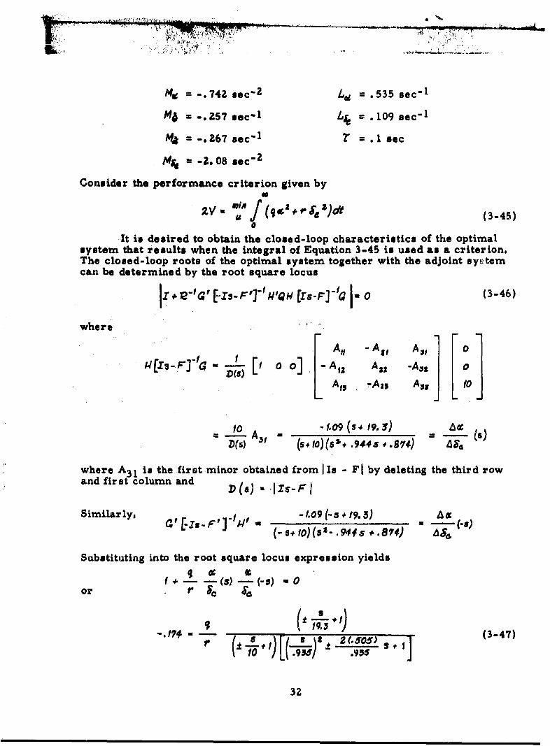
= -. 74 sec 2 L = .535 sec"I

2I 5 = -.25 sec-l Lie = .109 sec'l

A = 2.-67 sec 1 r = .l sac

fe = -4. 08 sec" 2

Consider the performance criterion given by

40

It is desired to obtain the closed-loop characteristics of the optimalsystem that results when the integral of Equation 3-45 is used as a criterion.The closed-loop roots of the optimal system together with the adjoint systemcan be determined by the root square locus

II " 2'G' [-,s-F'j-1''QH frs-F-J"1G I (3-46)

where

F1 Aft -All A$, 1 0o[I' o o] LA, A15 -A ss 0vo

A-s ss.) As- to-

to - 1.o9 (s1 ,90 3e ) ,de

D(s) (s.I0) (5 .94 , ,s

where A3 1 is the first minor obtained from I Is - F1 by deleting the third rowand flrst column and D(. .IZs-" F

Similarly, at -1.09 (-S+19.a) AX

(-$+fo)(sS-.944. $ .8iT4) 1156

Substituting into the root square locus expression yields

1*- (5)-(-H) -0or a

(~.to [.935 ) * (.95os ,

32

The actual plot of the locus of the closed-loop poles of the optimal sys- A'

tern is shown in Figure 3. Although the open-loop adjoint poles and zeros areshown, the locus of the closed-loop adjoint system is omitted for purposes of,1nr44ev- Tha 1 I.-- 1--,-------..... &n - •.A root iocus plotter, the

ordinate in phase angle (or damping ratio) and the abscissa is IsI. The "fishscales" represent constant values of the real or the i.mginary part of theLaplace variable a. The parameter of the locus is q/tr , the ratio of theweighting factors of U and ASe . It can be seen from the plot that as 9/ris increased from zero, the poles of the closed-loop optimal system appearto approach a damping ratio of r' = . 707 in the limit. In fact, it can be shownthat the excess poles over zeros of the root square locus approach a Butter-worth pattern as the qIr becomes large (Reference 3). It has been found thatthe approximation to a Butterworth is good for even small q/r values.

The root square locus plot illustrated in this example supports theintuitive basis for the selection of the matrices Q and R in the performanceindex. One may select 0 and R to trade off control deflection magnitudes forspeed of response. The root square locus plot demonstrates that a systematicchange in the selection of 0 and R results in a gradual, predictable change ofthe dynamic characteristics of the system. Regardless of the values of Q andR chosen, the optimal system will tend to have smooth, well behaved transientcharacteristics. It is believed that the dynamic response of a linear optimalsystem frequently is characteristic of the type of response that one intuitivelytries to attain when using conventional design procedures.

He also wishes to determine the feedback gains required to obtain theclosed-loop dynamics. These feedback gains can be easily found. The opti-mal control law is given by

S- - 1 "r'P - k%

and the optimal closed-loop regulator becomes

whose characteristic eqtiation is

1s-0 (3-48)

or, in terms of the aerodynamic derivatives:

S+.53S -1 .109 0L69 #.S 2.o-J 40 [k, kAL-0 ,o to-

or

sd. .5 -, .109

.r99 s 51.,.'r 2.0e 0 (3-49)

33

. . .,...'J..

6., ' + I .0- - 066416414 .. . .,r, , . .. ." " " " I so'. ..+"': in.. ..+ . " . .. ... 's... .... i• p ,, PP++ , -,,*i p'' ',i + + • ; ' ' ' 'i I Pv+' +, , , ° , i • •l l , *

a a Sd AP4 I S

- 14%- , * . i .+s + , -V - , . *,...,. • . .A ' , • . . .. . . . . . . .. . . .

10 0' Ill '1 to ) o •'s I' 4 11 i itti i% i I t l• l l # * l l l

'1, •,, 1',,• of 4 1 %' %" 's • ' " ,, 'i.. . , • ;/ .. " '.'.

. . . ... ' u. _ ,, .. .. ---- . . 4.-T . -__ ,a * *i a al i,.I P r..# '* , S -- .,* i# i, •

. .. a .. .. .. , .. ,- in ". .. ,-

is aam S P P a.

o , 1 , a- b: a a . 0. * , .

+a a' % . ",S,. :.. . .mill",

i 's -

",,I , ,*P'P**P° ' P -• O .*pat La p t , •, ' ,.i

4"1 'I ,,:, V,'<-1 \P.. . S**" , i,•r PT,a .- .-. ,-•

-, , ,; *' S a a" a p t,' a, S PI. , a., ,,** ' * - . "'* ' '

I's=

alaq *pa . ... . '. .. ,'•',.'.t ,,,,,. ,; ;*.0a,a , ,''p "' ., " ,';

Ia 4 ~ paala ' i ~ aaaIh ao | : .. aa .... ..... a P '.... ...S...... .. ,.......... . O ,.,',I,,', ',PP,:,

as, I *~~,,g,;,p,, ,,.' ' ,',; ,,ppP P paa ' , i p9, a',aa t t ,,

is . P

S".- -.' . , .. P. .... . : , -

app .,SS," ... p a.......a, ...... -

6. 1. . . .., .. . -,, .. .," ', .

T." 1 1. Iss

g~ I a at i~ ~ P a p P a - * -' IS li P ya d

....... .......... S

-, ,; , ,P 9 , ,P . . . . . . . . . . . .. . .

4. ',i, tp -s , , jp¶. --r ,: . A, i , yf a "~'

Io

_ A.

I : . : :, * . , ' ., -" -- .. s,:,I"a a t""" ".

u a . . . .

£ Pa.P.% pP.aP , " ." p ~.'+....." 5 P" =/. . ,p •IIp + # llllll I lI i ll llI I I •ill l ii .. i , . .. . , r '. o • ,~ .P. 1j9 ..a ,. , . <.._:

a ... ' ... ,p ;,p .,a I p," ..p s s. . ....... .. .. . .

p... ,..,P p... p p . ,.+ p * P P Ip . paa, . *

,, p,. . . .. . .p . . . , P pW ,. - , 11.- ' ,v' pp.' / .,I% -.- ; *a.'ps: p 'a, ' • ,CI,

, WI0 ",: , , *p .WW..,•.~',.,, o P .

a ... . .. "" ;;" ;"' ""P '° "° ""PP .... 'I *; "" "' "P".;. PP' '"""' '.. . .p

p,.. •, ,','',';pIP" . ....pP a t .P" , P,, ap:• ;,,a ,,S ', .. ,,' ,+,*S. . ... ... .. • - '', ep:''','','',. •oP',. I;,,;a , '•,'P, '... ,',',' .P , :

t' ll ,.." . , ... m .. .. . . ..... ' ......... "°" .... ... -,.. . . . ,,.,, ....a . ,.,pap ,pe ,P+,a, P ,; ,.a," * ', pp ,,pa ." ... . "..."'a -

a . ,:. % . - : 'rr .' . ...... .. . , . -. , , w, . . . . ,- , -..;,,a", U , , - , , , , , . . . . ...a; ., ... a .- , . , A .; S... ' . •

-.+ . , , . ' 7 .... o, P - ,." ".'p,. P ,, A ,,t ,. .-- , -, P VP- P,* .- . - .*

I- , .. . ... , ,o I ,

,,psl , . p ",i . ..- ' p . . ,. , • P ,. , . . ,, ,' ,; , ."- ' , l

"-"- ", ' , ." a' . 4pI. .. .

a .34

Z ., ,,p P$4PP

$ ! . 1..q o.'tta

The expansion of Equation 3-49 yields the characteristic equation for theclosed-loop optimal system in terms of the feedback gains.

Expanding. there results

S3* S 2(1106,& /04,.).- $(It #7 # aS91~ 20.5/1: 41094i)+ (8. Y9 , 8. 79 hj - A.3 kg - 2 /.k) th 0 (3-50)

From the root locus plot, Figure 3, a polynomial of the closed-loop charac-teristic equation can be formed. An an example. if I/#' = 10 were chosen,it is found from the plot that the closed-loop roots are obtained from thecharacteristic equation

(s + 10. 2) [S* 2(. 69) (2. -v4e ~(2.5s)* W0or

S5 13-752 s 42.4v + 66.3 -0 (3-51)

Equating powers of a of Equations 3-50 an-' 3-51l, the feedback gainsare found to be obtained from the solutions of the three equations:

/1.06 "10ki /3.72M,4 7 10,.5-9kAj 20. 5As - 1. 0 9 , n 4 2.4 (3-52)8.79 0 .79k,g - 10.3ks - 21-141 66.3,

Solving these equations yields the feedback gains

0.266(3)

k -2.Oo

The closed-loop flow diagram islElevator 4raf

Figure 4. Flow Diagram of Optimal Regulator

35

44 wv.

It has been argued that optimal systems are impractical because of themultiplicity of feedback gains required. However, it can be easily seen thatbecause the system is assumed to be completely linear, the state variables arerelated by transfer functions. For instance, A 0 can always be reconstructedfrom Ag with a lead-lag network, eliminatins the requirement for separate

Ac and A 6 sensors. -Also, because parts -of the system are at the de-signer's disposal, the feedback can often be incorporated in an altered design.For instance, the feedback 4$8--.z•z644 simply represents a requirementfor an actuator with a time constant different from 'r = . 1 seconds.

The above example is simple and could have been solved by conventionaltechniques, but the example does show that an optimal control approach givesan orderly treatment of problems. The optimal control approach remainsorderly for any system complexity.

3.4 ROOT SQUARE LOCUS - CONTROL RATE IN THEPERFORMANCE INDEX

It was seen, from Equation 3-8, that a variety of quadratic forms canbe used in connection with the quadratic performance index. Consider theperformance index that contains not only the square of the control but also thesquare of the control rate. It has been shown previously (Reference 2) that anacceptable trade-off between state variable excursions can be obtained for theoptimal regulator by trial and error techniques. If the control deflections aregreater than desired, say, to avoid amplitude saturation, it is necessary onlyto increase the relative values of R appearing in the performance index. It isfelt that the inclusion of a 4 quadratic term in the performance index willenable the control system designer to influence the relative control deflectionrates of the optimal solution. In addition, it will be shown that this additionproduces the equivalent of an additional lag term in the root square locus, andtherefore, in the optimal system as well.

Consider the problem whereby it is desired to obtain a design satisfying

the performance index

subject to the usual constraining equation, the original equations of motion ofthe system

The matrices R and T are defined to be symmetrical positive definitematrices weighting respectively the quadratic functions of the control deflectionand control deflection rates.

To obtain the Euler-Lagrange equations it is convenient to first gen-tp orate the function

[%V- AS iQ# U .04' rI~ 2! P a a] (3-55)

36

where X is, as before, an undefined column vector which is a function oftime.

The Euler-Lagrange equations then become:

m .- " -3 1 -

Performing the indicated operations yields:

(3-56)

a, •(eta #RA"S)# AA#4

Combining the Euler -Lagrangeo equations with the constraining equa-tion yields:

(3-57)

The multivariable root square locus expression is desired'for thevariational set of equations (3-57). To find the expression for the ciharacter-istic equation of the above set of equations, first take the Laplace transformand obtain:[ S-F] 0 eG (0)] F

-0q'09 (fz.i'j 4F 0I~T VS()~ [ -AM (3-58)

L 0--r' I o)-r"'( L(,)J , ( -( o)&JThe determinant associated with the matrix set of equations (3-58),

when set equal t, zero, defines the characteristic polynomial of the optimalsystem, which includes the stable solution and the adjoizt, or image solution.

37

It will be convenient to use Gauss' Algorithm to find an equivalentexpression to the determinant of Equation 3-58. This determinant is of thepartitioned form

l C as 0 's 0 :0

1 0 COSp C53where Cij is a submatrix within the determinant of a partitioned matrix.The followving transformation does not alter the value of the determinant ifC01 is square and C01 1 0.

C, 0 C,0 C,, 0 C-,

0 C.4 2 Cas 0 0 s 1") Cswhere

S. •(J--i cot C1 it"'CIB ÷ r,

In terms of the matrices of the determinant of Equation 3-58 the re-sult is

(.Is-F] 0 7a [I Fl a i-PON. -[Zs.P'j7 0 " o -feP -[Y.'J•'[1s4T', (3-59)

-T'0 *Is&' -7 -r'-C' Is -T' (9

Repeating the Algorithm:

a it 0 eta Co, 0 146j~~ ~ 0~j a," 5''

c0 al,) 0 0 W,1 '

where c,,fw- [,], C,13 (tC,

- [r"'a'] [- r.-r,]" -, [/'.(xe-F)-,a]. Zs,.-,'R

Equation 3-59 finally becomes

- s-F 0 o -a [,s-v] 0 -c

0 .- 4,411 [.19-r 0 0 [-1,-F] JW',V[XS,••OQ 0 -T"-,'[zwr.rJ 0 0 0 ("'QVEs-F'""[A.Y8"•Q

38 -''- T-•'t0}

which can be written as follows:

irs d~r~~ 'I(I' -')~T-C'(IsI~T'./QY~s-1~0 -0 (3-60)

Because uIs - FI and I-Is - VI are by definition square and not equal tozero except at thin npnn.1t%^n ti;, -- a ....------------. '--"-------- --- I

or (3-zsr- I--, . .s.. (3.61)11 .tls'T"' ~)'T"'G' -I6s.P'] '/-'Qi/f[Is- FJ't0I 0to obtain the closed-loop roots of the optimal system and its aijoint. Noticealso that for this performance index, j1s 2-.r'fRI defines additional open-looproots.

It can be seen that the W'TJ additions to the performance index procucea slightly different expression for the root square locus, with (is -r-'1" -Tr1

replacing R . This has the effect of adding additional poles in the root squarelocus plot at the values indicated by the expression Ze2-T'fel-". The effect onthe optimal closed-loop system is to add first-order lag networks, one for eachinput or controller.

3.5 ROOT SQUARE LOCUS - OUTPUT RATES IN THEPERFORMANCE INDEX

Consider the performance index containing only the output rates and thecontrol deflections in the performance index, i. e.s

where M and R are defined as positive definite symmetrical matrices weightingthe individual terms of the performance index. The constraint is# as usual,the equations of motion

SI 4 X (b) (3-63)

Substituting for j 'in Equation 3-62 yields

'2V f(*'HA1,Qi + 'Rus) dtC

The Euler equations associated with the solution of this problem are, as before,

pa d la Pe J

where

The Euler equations yield

+ pAF~" M/I 4 -0 (a)

"V * 'Z ,0, hence tA -- 'o' Z (b)

39

Combining Equations 3-63a and 3-65, the result is, after taking aLaplace transform

L[-rSJl.wts.J [-X.-F.Jj L1sJ L -H1'm~xs % (00AJ (00 J j ')

The determinant of Equation 3-66, when set equal to zero, defines the rootsof the closed-loop optimal system and its adjoint.

Again, by using Gauss' Algorithm, it can be shown that the root squarelocus becomes:

.IX] '( '-I.-""'WMI4.-FJ"cI- 0 (3-67)

It is clear from Equation 3-67 that zeros are added to the root squarelocus plot at the origin. Otherwise, the expression is the same as Equation3-25. Adding zeros at the origin of a root locus plot is equivalent to obtainingthe locus of the derivative of a transfer function. Equation 3-67 can then bewritten jI-s'~J[~cs [~() w

The Riccati equation can be easily obtained for this particular per-,formance index by substituting * u •'+t in Equation 3-64 before the Eulerequations are obtained. The function £* becomes

U U

S-F".'M./' ÷=t#M#.÷ " "-'• -

40

o rM

X 32X1 o()MWS

• i I III I I I Ir

The Euler-Liagrange equations, together with the constraining equation, become:

j +'•, + F ''*'MV F, + F*'#JfNM a -O (a)

Q'#'MWA1-z + 1''M144G, ] JP V - 0 (b) (3-69)

Solving Equation 3-69b for t yields the optimal control law

U, --'P a w -.. . '.* 1 (3-70)

Now substitute 3-70 into 3-69a and 3- 6 9c and obtain

-F YI 4 7 . [4'A#'o X I x" JG 'A .c ' f' m r xrIj •0 (a)(3.71)

Let A. PY , •" P• , where P is a constant matrix, and multiply 3-71a by P,yielding:

- *P4 [G/'w - Pro!c +~ paPas- r4 , G'" A wwswrq oPi + P'*, O'W'AN- F'WAGjC'#'AN4/k 91'1[6 PV *cWMAlFstJ , 0

Finally, eliminating P4 in the above equations yields the Riccati equation

P [F-GA']J.(-B'A'-G']ji* [C-B'A"B3-PGA'G' P ,&0 (3-72)

whereA aG'H'MHG+R

a G'H' MHFC a F1H'MHF

3.6 ROOT SQUARE LOCUS - MODEL IN THE PERFORMANCE INDEXThe use of a mathematical model appearing only in the performance

index to describe a desired system matrix was first suggested by Kalman.The technique is as follows. A mathematical model is defined

S.z,•(3-73)

where y is some fictitious state variable and L is the system matrix of thedesired system. A performance index is specified of the form

2V uJ(.SI Q4Ll4'n (3-74)

0

It can be seen that if the system output rate j behaves exactly as themodel, the first term in the performance index, s?- kg , will be sero. If thecontrol of the system is such that feedback can force the system to behaveexactly as the model, the regulator in the limit (i.e., as IQI/!91 -4 • ) will

41

II

behave exactly as the model. To obtain this condition, if it is possible, oneneed only consider the performance index

do0)%/ .0 f r.. , .1.',a r.. -i .. i , A - %

j LY 7 YJ L I wTJ b0

If the model can be exactly matched, an optimal solution will simplifysuch that the optimal feedback control law becomes a set of fixed feedbackgains. It should be pointed out, however, that the case where the system andthe model are exactly matchable is the rare exception rather than the rule.In general, it requires that L, F and G be of the same dimension. An artificialprocedure would be to have the number of columns of the G matrix equal tothe number of non-matching rows of F and L. For instance, if F and L wereeach obtained from a transfer function, then F and L can be written such thatonly the entries in the last row of F and L differ. In this case, a single con-trol variable, with a column G matrix, may be sufficient to exactly matchthe optimal regulator to the model. However, exact model matching in prac-tice often requires large or violent controller motions. The inclusion of the

als'u term in the performance index allows as close a match as possiblewithin allowable controller motions.

The root square locus for the model technique is obtained in a mannervery similar to the previous developments. The performance index is

" ~0where

Substituting for and • yields

0

(3-76)

To assure that the integral performance index contains quadratic forms,note that the two bilateral forms- '/'QPL/Ao/ and -%'/#/%10/1 constitute thesymmetrical part of-2V•/'QL1V/x and therefore can be treated as a quadraticform.

As before, the Euler-Lagrange equations are

day_ ax d/ (M)-

42

where

+ +'.(-. ÷ " Gs)

The Euier equations become:

A. , Alg'aQ~ ý/ * f Y - A! I/ OV"a V0 (a)(3-77)

Ra + OA - 0(b)

Solving Equation 3-77b for u yields the optimal control law

The two equations that describe the realizable optimal system and itsadjoint are:

F_-se + a- 14 = 0F AIQ A X A1'QZW j 1QAjj#. 1"L QZAIX= 0 (3-78)

In Laplace transform form, these equations become

,WL [x-s- J I(f) M= [Xi xW ,o4 (O)J - h/'(QL. #L01014is(0)74oj(0)

The determinant of the left-hand side of Equation 3-79, when set to zero, de-scribes the closed-loop poles of the optimal system and its adjoint. UsingGauss' Algorithm, as was done previously in this section, a convenient ex-pression fjr a root square locus can be obtained:

[r+ -R - , s-L1 xs- Lj*/(Xs-,C'2 P (3-80)

which again is of the general form

DIFIt can be Peen from Equaiion 3-80 that the elements of the model ma-

trix appear in the root square locus and contribute to the zeros of the rootsquare locus. In fact, the order of the numerator NNq is generally increased,such that NRq and OD can be of the same order.

If this is the case, the elements of the Q matrix can be chosen such thatthe zeros of the root square locus are the eigenvalues of the model and ad-joint, i. a., I Is - LI and I -Is - V and the optimal system will, in the limit,(ioe., as 1Q1/1J2 becomes large) have closed-loop poles that are identical tothe model poles. However, this procedure would in general require somenegative values for the elements of the Q matrix. The system can no longerbe described as "optimal" as defined in the original formulation of tV.e problem.

43

I

However, if one obtains better model following by selecting negative q *I*-ments, the distinction between'optimalfa nd'non -optima? becomes trivial.

3.7 MODEL AND PLANT EXACTLY MATCHABLE

It is not obvious in the previous formulation of the model performanceindex problem that the plant will. under certain circum...tancer, actually matchthe model exactly, A slightly different formulation of the problem will showthe match more clearly.

Starting with the same performance indexdo

0

Substitute for y and

and obtain

- *

+ u 0 '4 Q& -L9 ,0 [ A 9ý4 A2 d (3-81)This performance index is of the quadratic form

V= A - 0

where

A is [ -4

C - O/'Qj010 *

The Euler-Lagrange equations are obtained in the same way as before,using the function

"de +

The Euler equations are:

(3-82)0 (b)

44

Solving Equation 3- 71b.

(3-83)

The two equations that deocribe the clot-d-loop optimal uyutern and itsadjoint are Equations 3-82a and the original plant equation, with t4 substitutedfor t

.F +Ax - SC'13's - VC't0',& -0 (3-84)

After writing these equations in Laplace transformed matrix form,there results:

fro~- F 1* r c s if- L1V] (3-85)

-(Is L_ _L_ jIt will be recalled it was stated that if the plant and the model can be

exactly matched, the dimension of F and L must be the same, and that, ingeneral, the number of columns of G must equal the number of rows of F andL. Also, the W&'Q term in the performance index can be dropped. There-fore, let R = 0, H = I and dim. F = dim. L. Then HG is invertible and thematrix entries in Equation 3-85 become:

,:- rs-F+ a(G'Q&T'G (F-L." =- Is-I.

a -fr3 '-D4 -,.1'daGa'qwGT'Q'J

A - BC-'W - 0

Substituting these values into E uation 3-74, there results

F 1 (3-86)L 0 -z.-,.j L,, _j =L,The determinant of this set of equations, when set equal to mero, is

Irs-L.II-Is-LL1'1 C 0Therefore, the optimal regulator has exactly the same characteristic equationas the model. The optimal regulator satisfies the set of equations

and the model dynamic characteristics have been exactly matched. Under these

45

I

circumstances, the optimal feedback control law is given by

When the plant and the model are exactly matchable, optimal techniquesare obviously not required to obtain the feedback law which produces the match.The importance of this technique lies in the fact that if the feedback gain mag-nitudes were restricted, linear optimal techniques will enable the designer tomatch the model as closely as possible in the integral error squared sensewithin the allowable control motions. It has been repeatedly demonstrated thata near match in this manner produces a well behaved, smooth approximationto the desired model system matrix.

Two examples will serve to demonstrate the model-in-the-performanceindex technique under the circumstances when the plant and model are match-able and not matchable.

Example 1: Model and Plant Matchable

Let the system be described by the first-order set of differentialequations I 1 0 f L, 0

[11 [4 f J (3-88)

0 f '

and let the model be described by the fictitious set of first-order linearequations

= (3-89)

Notice that the plant and the model vector describe an orthogonal setand the matrices differ in only one row. There is one controller, so it canbe hypothesized that these sets of equations can be exactly matched as JQI/I•ibecomes large.

Equation 3-80 is the expression for the root square locus for thisproblem.

ji .•'"'Uts-P-'J"'(-I,- t'JQ•rs-LJIJCzs-PJ'j-o 0(390)

46

It has been shown previously that the ratio IQI/j/l is the main par-am eter of the root anua. i ....... . . w abuui e values ot u or

R. For convenience, then, for this example choose

Q ]Calculating the entries in the root square locus expression:

iI (- Fj"ig = the generalized transfer function matrix

1~ F0 M~ ZF(m S~~z

Similarly,

ga 5 ih o (- s) 5 s

L,.•,, o),f# ,(,.•t.)(-,.,)

Substituting into the root square locus expression yields

rlg -... .. 4 (s-0)1L

[i~ ~ 51L515 ("it fra)&*s)J [.

or S #g#1 eJ 9 (8.A Jetg~

or r (s) D(D (-(s)

or Oti D A, (s) DAF•

r IrS) DP &) (3-91)

where D/.(s) 6) -IszS , Dj.('S)" S"A-g5#JAI

47

S...- " - -|

- •

4,16C - i / GaU aa J arc Lim~

characteristic roots of the model and its adjoint, the root square locus willoriginate at the poles of the plant and terminate at the model roots. The op-timal regulator and the model will be identical as I/r approaches infinity.The feedback gains will, of course, be finite.

To provide an actual numerical example,* letE0 1] -0 1: - --1 -2 25 -70 0,o

The expression for the root square locus becomes

r(+ s r- ) 7. 5 0 (3-92)(624 2s%, f) (0 -ZS +,)

Figure 5 is a root square locus plot performed on an ESIAC root locus plotter,which semiautomatically obtains a root locus on a rectangular plot, with damp-ing ratio or phase angle of a as the ordinate and absolute value of a as theabscissa.

The parameter of the locus is f/t" and the plot shows that the plantpoles migrate to the model poles rapidly and in an orderly fashion.

The optimal control law, in the limit as I/" -0 to is

- -5 -207_ -24 -. oI L

or

UO - 24 "Y,, "5: o7" z.

This example was used previously by Tyler, Reference 12.

48

Oua

- w I. v 0-. -- IA. .

I 1 14 4 6 1 .%.o P. m l t l o % 0 0' 4 V. 4 -- I A d

1 104 1 1 0S ! 4 * * g * * I 1 % I I I s A *1 0 i ,

g . 4 ~ P-&VA.6 O I P *I. *AI

I~ ~~~ ~~ ~~~~~ .. . .l~ l l . . . .d~~l i J . .t ~it ~ I A

A.* ti IM !

*~~~~ i Ii1.4 01% V Ah I II I s ~ % I I I - A i It oI 4, I t 1 4 11 V% 't % It 0~. b~ 4A ~ ~ ~ 9~ t . . . .J ; VI I A'' 't Vir's 0* A IO l~~5155

W% liU O~ t 4 I4 I t t I I %0~% A14 it ' .ow I .1 ~ *tt ~ t t I -C i

0 1- 1 4* soIS . - * 4O 4

I. ~ ~ ~ ~ ~ ~ ~ . 44 44* ~ ¶ 11' I

1 t**~1tt -16, -o I... 1 414 .

Vio SI t sit tI I ki~ lil lilt lii itt 1. 1,.,tl . ,

. I it S ItitI AtI

. . . . . . . . . . .... a

i44 loa !4U t#4 1 1t, I i a C

7- L th . .. .I

4 4)

1. t4i1t 0. A

49.

VSS

d --a . - - . ....... . .. .... . . . ... . . . .. . .... S. .i. .

J~A~a~a~ . £'VA~ULl U,,AU £-LazL Cj.uL b© LV=i.,IUhU AU5LLU•=,I:•

As a second example of the use of a model associated with optimalcontrol, it was decided to use a somewhat more realistic system. The simp-lified equations of longitudinal motion of a high-performance military fighteraircraft were hypothesized for the plant. A model system matrix was specifiedwhose natural frequency and damping are such to satisfy acceptable flying qual-ities. Ntuora1 frequency and damping are, of course, only two parameters ofmany that are used to define acceptable flying qualities. Other parameters,such as the slope of Cq. vs. a curve are equally important.

However, the model-performance index problem as it is presentlyformulated allows only for a change in the system matrix, i.e., it is possibleto change only the state transition matrix. The transfer function matrix ismade up of the output matrix and the control matrix as well, so the transferfunction of the closed-loop optimal system can be affected only to a limiteddegree.

If the above logic is extended to the model situation, it should be notedthat the performance index for the model case is specified in terms of errorrates between a desired response and an actual response. Since whatever ap-pears in the performance index approaches a Butterworth response, it is clearthat the error rates between the model and the aircraft will be smooth and wellbehaved, approaching zero as the weighting on the error is made very largewith respect to the control.

It is not possible in this case to exactly match the plant to the modelwith finite values of error and control weighting. Assuming that the importantvariables are angle of attack and pitch rate, it will be instructive to see howthe closed-loop roots of the optimal regulator behave as a function of the rel-ative weighting of the 4 6 and A X error rates and the ratio of the errorrates and the control deflections.

Assuming straight and level flight, the short period equations of motionabout the stability axes can be written:

- $e~ pitching accelerationAW # d t4A equation (a)

Le 60( ' L a• e flight path velocity (b) (3-93)

equation

The elevator actuator dynamics were assumed to be

- 2 reV7 so + ed 2

These equations of motion are easily put into first-order form bysolving for L& and substituting for 6 & in the pitching acceleration equation,Equation 3-93b.

In matrix form, the first-order differential equations of motion become

50

AG -M&1-,% M6 M , M&-M L, 0 0

S0 0 S 0 C (3-94)

Se 0 ACT

The model chosen is of the form

, L -", L, M6.Mki L#,, (3-95,

and the following derivatives have been chosen:

MO = -. 742 sec"2 Mg = -16.0 sec" 2

M6 = -.257 sec-l M1 W =-2.9 sec'l

-. 267 sec- I Ma = -1.0 sec-l

S-2. 08 sec 42 LOW = 1.5 sec" 1

.535 sec" 1 &LAcr = 20.0 rad/sec

Lle. .109 sec-l rfr = 1.0

The flight condition associated with the derivatives listed above is oneof low speed, low altitude power approach. The short period natural frequencyis 0. 935 rad/sec and the short period damping ratio is , 505. The model hasa short period natural frequency of 4. 5 rad/sec and a damping ratio of 0. 6.

Substituting the aerodynamic derivatives into Equations 3-94 and 3-95yields, for the F, L and 0 matrices:

-. 599 -. 524 -2.06 0 00 0 0 f 0

0 0 -400 -40 L0 (3-96)

= L" -9

S~51

It is clear that the closed-loop optimal regulator -(F- r)x cannotbe forced to have the dynamics of the model under any circumstances. Theaircraft and the model matrices are of different order, and even if L werewritten as

Sr - 1. 0 0 t 0 0S-i4.r -3.9 0 0 jz, .12Z 0 o

0 0 0 0 = 0 0 0 0

0 0 0 0 0 0 0 0

to make the two matrices of the same size, all four rows of F and L are dif-ferent, and as has been suggested previously, at most, one non-identical rowof F and L can be matched with one control variable.

It will be instructive, nevertheless, to investigate the closed-loop dy-namics of the optimal system that match the model as closely as possibleusing the quadratic performance index as a criterion. It will be seen that theclosed-loop poles originally associated with the actuator increase in frequencyand approach • = .707 while the poles originally associated with the shortperiod roots of the aircraft tend toward some frequency and damping inter -mediate between the frequency and damping of the open-loop aircraft and themodel.

Let it be assumed that it is. nominally desirable to match the closed-loop aircraft to both 4ac, and AO,. The following H, 0 and R matrices canthen be chosen:

Ha0 2 0 0 L 2]

This yields a performance index

or

0 (3-97)

It has been suggested that the matrix H must be the identity matrix (IIfor a proper formulation of the model-in-the-performance-index problem.This requirement doesn't appear to be necessary in this case, for this wouldmerely add two additional terms to the performance index, mainly, 5I5eThere seems to be no apparent advantage to the inclusion of these two termsin the performance index of this problem.

4', 52

L!s

Returning to the problem with the performance index of Equation 3-97,the expression for the root square locus is, as before

11+ "[-z,-'"'- ,']( [., -LQ (is-ti /./(s-IJ'G/ - 0From the definition of H[I.-F'Jt and G't-Is-F'J"T', the transfer func-tion matrix and the transpose of the matrix with a replaced by -s. there results

/[Is-F']Jt . r 1•''+)k'jg (Vg S~v

(3-98)

ATZ-s) ei Vj

where A- ('rS. 1) numerator of 74' (j) transfer function = A

lei (r, s numerator of 611, (s) transfer function = A/j

-,. v) = numerator of "/ (-s) transfer function =N

i(-Z S# 1) = numerator of / (-S) transfer function =

In terms of the aerodynamic derivatives.kl" Mid Ls it " e"• " .-. •o

Seg4~j~ 0-11 4 LW t03

S(s) : denominator of the transfer functions of the aircraft

actuator aircraft

F (- s) = denominator of the transfer functions of the airplanewith a replaced by -s

53

00 --- - - . - - - . - - -A ao

Also,

I. ]61 L]

-¢,(u-ft,) *,-iJt f (3-99)

Substituting Equations 3-98 and 3-99 into the expression for the root squarelocus, there results

((O.c 7)' [NoNo .15 ~NVF N6 i's ~ I " =R l 0 (3-100)PZ) 1FS) P4-)

Equation 3-100 shows that the expression for the root square locus isof the form

The zeros of the locus, NN, are a function of If and Is and there-fore in themselves constitute a root square locus expression, which is given by

Alf X 0 1 -. 9 /V R J, 1-g J (3-101)

After substituting for .8 ,' , Pg# and A;u and rearranging to ob-tain R/ as the parameter of the locus, there results

0 1 _ NsN +f)&Nis4y N ~ (3-102)

Equation 3-102 defines the zeros of the root square locus, that is, theroots at which the closed-loop poles of the optimal system will terminate.

After substituting for the numerical values of No , R, , , , ,

-I, -t, , and Iss , Equation 3-102 becomes

#, (- -) (3-103)

qý ( S t Y.'7jSU)

The dotted lines of Figure 6 show half of the locus of Equation 3-102as a function of q/8 . The reflected, or adjoint, part of the locus has beenomitted for clarity. As can be seen by the figure, this locus defines the end

54

41 A- 0~ V-.Jv~~ -WP _ .0*w 4 A% 0

~.. ~ ~ I A el I .. f

I - I fI -0 0-0f "41 -0 -It 1. 1 p v S .1 1S f I I M

Il~~~~l' PIt 0I ff1,10 , . ,:. . . . . . . . . ..

0lf 1 * 0 ffp of o t IS 0lf~f~ - I Vt 'tlf Of - I 111

I* fA^" fte I 0 I ~ L0 1 1 f t~.&L~l k: v OI~ 0 0 0 46 * I#-4 w % A .-- 6 W a,4 4.

*f~ f -' ff ff f ll f fI~TfI % I~ I. . I .I% l l

Offi f f fl~76- S f~f~ Isll %I 1. .14 f1ff - 1 L .100ff0 %IfSf~IW ~ ffl ff04 ~ If .,6f~a -fff

* h..4~0fA,

P! mmw I1E ff ho 1f , I I DlI i161*~.fII. Ef ff fe 0,661 1 1 i~ I

Ofi s-ffffl f rif-ffT 1-f.06SIff~~f~~lI IIfO ~fffll I fffIE

* ~ ~ f f P A A I ~ f ~ f IA t. U A I I *

L .1

.

............ 4=I r .. Iff ~ f . f1I

11ff -, I lffl ICOfIIf d II 5 f11I t IL ffl -

I ~ ~ ........... a - ........~ S I - I f l S f f f I I fIlff~ ~~ ~~~~~ a ll f1 R *.0~f

ff~~~~ ff*.4 ~~~~I

is.f

f .*f .

~ ~ *~ .

tllf~~ ~~~ ~~~~~~~~ ItC)?V ffI I .f-qff f/ Ifl9f0 I

* ~ ~ ~ ~ ~ ~ -flf 45f~*f-.-5 . f

,bd~l -~ ilf fff4

l~~ff., 0 5 fI0 f54 . .01 ) f l l ff f i ~ f .ff60 I~ I I I ffflfftfAIs f fl

io s l f f _~l~llf6

If ~ ~ ~ ~ ~ ~~C C)l11fIIfl(¶fIf1

.5 .5 ~ I

*I~ffIfI 111,.1fllff4- f5

points of the locus of the poles of the closed-loop optimal system. The pointwra,,m~, Ai 0i.. 10. =s f 4 o .. * ,h , ..4, 4,L4. ..... I ., . .. - ... L.-. - •, .. .

rnalrnA4L ha -0 the A..-t wols 'AmYW- w&at'6v..-ALAiulU ILc L ierm1(; - if a -Ats " )2 had been omitted from the performance index, while thepoint 4, /9. -w in the end point that would have been obtained If the term( It- at - Ats A P were omitted from the performance index.

The locus of the poles of the optimal system can be found once a valueof go/f& has been selected. If a value of 9,/9f = 100 were chosen, Equation3-100 can then be used to find an expression from which the closed-loop polescan be found. Substituting 3 .eOfqt and the values for No, NO , Nj , NJD(s) and D(-s) into Equation 3-100 yields

-. 00110 10i[9 2(. 56) (4.r9) 8 (4,t9)' (3-104)r [S 1201 3' aSA 2 (. SOM)93608(9 85)J

The locus of the roots of the optimal system, given by Equation 3-104,is shown as the solid lines in Figure 6 as a function of the ratio 9, /t. Again,the adjoint system is omitted for clarity.

The original intent, of course, was to match the system to the modelas closely as possible. Because the model was second order and the aircraftwas assumed to be of fourth order, it was known at the start that it would notbe possible to produce an exact match. The model has a natural frequency of4.5 rad/sec and a damping ratio of a 0.6. It can be seen from Figure 6that if 9f /48 a 0, two of the closed-loop roots will in the limit have approx-imately the same damping ratio, sw a 0.6 as the model, but the frequency willbe less than that of the vodel. If 9f/l, = ao , the natural frequency of two ofthe closed-loop roots will approximately match the natural frequency of themodel, but the damping ratio will not match. In either case, the two excesspoles, originally associated with the actuator, tend toward a damping ratio ofapproximately 0. 7.

This example attempts to answer the question "If the model roots cannotbe matched exactly, how close can they be matched?" The answer, as dem-onstrated by the root square locus plot, is that they can be matched fairly welldepending upon how the individual errors are weighted and how much controleffort is allowed. If the available control effort is limited, i.e., if q0 /ris finite, the roots of the closed-loop optimal system will still systematicallyapproach those of the model.

56

_I,

SECTION 4

THE SINGLE CONT~rP MT.W. I V1,,11 SYSTEM

4.1 INTRODUCTIONR. E. Kalman stated that the major contributions of linear optimal con-

trol will be to the conceptual design of high order multi-controller multi-output control systems. It has been shown that the resulting closed-loop opti-mal system is stable and well behaved, with an initial condition response thatalways tends to approach the response of a Butterworth filter as the weightingof the error portion of the performance index is made large relative to thecontrol. The control system designer need only select the Q and the R ma-trix, perhaps by trial and error, or possibly tising root square locus tech-niques, and, using a large digital computer, an optimal control law can becomputed.

A major limitation of the method just described is that the relationshipsthat exist between the parameters of the performance index, the closed-loopdynamic characteristics, and the feedback gains are only qualitatively known.The multivariable root square locus, developed elsewhere in this report, der-cribes in fair detail the relationships that exist between the performance indexparameters and the closed-loop poles of optimal systems, but no such clearand straightforward relationships are known to exist to determine the closedform connections among the Q and R matrices of the performance index and ,the feedback gains of multivariable systems.

When dealing with single controller systems, however, the relationshipsthat exist among the performance index parameters, the closed-loop optimaldynamics, and the feedback gains are not difficult to obtain. The single con-troller class of systems is not insignificant or unimportant and it will be in-structive to demonstrate the essential relationships of single controller opti-mal systems.

4.2 FEEDBACK GAINS AS A FUNCTION OF Q AND RIt will be found in Section 3, Equation 3-20, that the optimal charac-

teristic equation and adjoint are given by the determinant

I s- o ' If

-W (4-1)

or by the spectral factored product

Because the development here is restricted to single controller ys -tems only, the zeros of the optimal system cannot be altered by feedback gainsonly. The zeros of the closed-loop system will be the same as those of theopen-loop system, and only the denominator, or characteristic equation, willbe altered. Equations 4-1 and 4-2 are sufficient therefore to completely des-cribe the optimal system and its adjoint. Equating the two determinants will

57

therefore yield two polynomials; of which the coefficient of one is a functionof U and A , while the other is a function of the ieedbacK gain &. iquating thecoefficients will then yield a set of equations relating the feedback gains withthe Qelements of th Q and R matr~ces. L• addition .e.au the relation ahip;between the dynamic characteristics (such as closed-loop natural frequencyand damping ratio) and the feedback gains are known, these dynamic charac-teristics can be also related to the elements of the Q and R matrices.

Consider the plant that can be completely described by the followingtransfer function C-• (S)-

' -6(546) (4-3)

whose state description can be written:

(4-4)

Consider a performance index for this system of the form0o

2 V (9, qz , ,'s r.•) to (4-5)0

The characteristic equation for the optimum and adjoint is given byEquation 4-2.

0 $-" 00 s 0

S~(4-6)

or

The closed-loop optimal system matrix is of the form

S-bk[ (4-8)

, ,• 58

L~ .... ---- L---• ... 4".

After substituting in Equation 4-2, the characterintei •onintalen _ 1 44w-.

upiimai system becomes

I- , -- #+bh, - 0 (4-9)÷bk, so• i a I 00-s -s#4,,bhj

or

9-s'-2bk, #'at 24Mb, -b'h,'].b'k,' -no (4-10)

Equating the coefficients of powers of s of Equations 4-7 and 4-10, thereresults a set of equations from which k can be obtained as a function of the un-k n ow n s o/ r an d f t/ P •

-2,o 2ah, . (a)r (4-11)

. .. - (b)

The polynomials, Equation 4-7 or 4-10, are of the form

2wy 4r 0#41) #Wfp [grz 42~d5f,1S 2p'~,, 10 W"' 0so that the solutions for kf and kt can be expressed in terms of 9,/r andIsb- or the closed-loop natural frequency and damping. The characteristic

equation of the closed-loop optimal system is, from the first determinant ofEquation 4-9,

.2 (ab -6 (a 64A) 2 + (4-12)

Because stability is Waranteed for the closed-loop optimal system, thecoefficients tt÷bha and bk, must be positive. The proper solutions of k, andks from Equation 4-11 are

'4 "'gZ 9 b2 ' (4-13)b b V ,' a'

If it is desired, Equations 4-12 and 4-13 can be easily manipulated toobtain the closed-loop frequency and damping as a function of 9, /r and 9/ Ir

It can be seen that direct relationships do exist between the elementsof the performance index, the closed-loop characteristics, and the feedbackgains. The matter of obtaining a particular optimal configuration is simplya matter of the proper selection of the performance index.

59

14.3 PERFORMANCE INDEX FOR RESTRICTED FEEDBACKUsing the same dynamic system of Equations 4-4 assume that it is de-

sired to obtain the form of the performance index that yields feedback from. the variable -x only. That is to say, position feedback only is to be allowed.

What quadratic performance index will yield position feedback only? With thisrequirement in mind, Equation 4-9 can be reformulated# settingk 8 = 0.

a -1 s -Mv .0 (4-14)

b s~a I 3-4

or (s*.ias, .M,)(s*-., ÷ hk,) - C

Equating coefficients of Equations 4-15 and 4-7,_( (a)

AL (b) (4-16)

Eliminating k, from Equations 4-16a and Equation 4-16b, the requirementthat position feedback only be allowed is

bs

or 4#

2 (4-17)

and the resulting performance index is0

2V 9 us)d (4-18)

Consider a numerical example of the limited feedback problem. Letthe dynamic system be represented by the set of first-order equations

= ÷ U(4-19)

and let the performance index be

060

0 60 s m m s

The erhnivt*--i ."t" 4-'-s- U "& tii up•irrmi system and its adjoint isgiven by substituting in Equation 4-7

3-5Z (4 - 4 • )+ 49, .0 (4-21)

The locus of the roots of the optimal system and adjoint is given inFigure 7. It can be seen that the negative sign in Equation 4-17, as selectedin this problem. yields position feedback in the conventional degenerate aense.The Butterworth distribution of roots is not obtained, however. Two obser-vations may be made from this example:

1s A Q matrix that is not positive definite or non-negative definitemay still yield a stable closed-loop system.

2. It appears that the system may have closed-loop poles otherthan those approximating a Butterworth distribution ifelements of the Q matrix are allowed to be negative.

+3jI

!

j2 I

k, '2 q11 4 Ik 1 .4'€' q,1'2 I

I

k, v I q"1 '.25SI

I

i '.K5 ql'.25 -

.- 2 + 1 + 2

OPENtLOOP

1-12

OPTIMAL SYSTEM ADJOINT SYSTEM

Figure 7. Locus of the Roots of the Optimal System -

Position Feedback Only

61

LI • i * -" r . .. . . . . . .

Conds;ar one otier variation oi the singie controller problem ot thissection. Up to this points the resulting closed-loop optimal system has beena regulator, No Liputs other than initial conditions have been considered.

Othex inputs can certainly be considered, however, merely by incorporatingthe'state variable description of this input into the plant as an uncontrollablepart of the plant. Consider, for instance, a step input. This step can be des-cribed as a first-order differential equation as:

ji =0Attaching this vector to the plant of Equation 4-4, there results the system

[•] :0 0 II E 1 [ (4-22)

42 _ 0 0 -a L_16 b _

Because it can be desired to minimize the error between the step inputand the output, a performance index of the following form may be selected

ZV 2 ra 2'Jdtor

zV - f(V• - 16f q + ,a ')Ol.z)t (4-23)0

The resulting optimal system will be of the form indicated in thesketch below.

If the determinants of Equations 4-1 and 4-2 were expanded and thecoefficients were equated, it would be found that ki could not be obtained inthis manner. The di can be found from the Riccati equation or by usingS. S. L. Chang' s approach. If computed, it would be found that ki = k, . It

would also be found that the closed-loop part of the system is still an optimalregulator.

62

It has been f(odnd iij general that the closed-locp regulator part of thesystem is not a funrtion tof the excitation to the systern. The input gains to theSvsteri, such as the ki of thl above sketch, will be a Cti:ction of the dynamiccharacteristics of the sysl:en excitation. This can be '.2asily understood be-cause each of the state variables required to describe the input excitation con-tribute to the closed-loop part of the system.

'rhe input problew ;n nd other problems disc ussuul in tbis section demon -strate that there are definite, fixed relationships that e.ist among the param-uters of a quadratic perfirmance index and the characteristics of the optimalclosed-loop system. The simple examples have shown that much of the con-ventional control terrmuinology, such as natural frequency and damping ratio,cani be expressed in term, (if the parameters of the quadratic performance index.

It was not tlhe inlteot of this section, however, to show that everything(lone by optimal control could be done by conventional techniques. Optimalcontrol yields a method whereby systems of large dimension and many inputscan be computer designed, with the knowledge that a positive definite matrixR and a non-negative definite matrix Q yield a system known to have desirablecharacteristics. It thcv two conditions are met, the system is guaranteed tobe stable and the response of the closed-loop optimal system rapidly approachesthe response of a Butterworth filter, smooth and well behaved.

Possibly the most important characteristic of linear optimal techniquesis the freedom of the designer to qualitatively determine the amplitudes of themotions of the controller inputs to the system. If the control motions of alinear optimal design are too large, it is necessary only to increase the weight-ing on the controller in the performance index and the next design will havelower control motions but at the expense of greater error. In either case, theintegral of the square of the control motions is minimized. This means thatlarge excursions of the control are discouraged for any weighting of the con-trol in the performance index. In fact, S.S. L. Chang (Reference 3) demon-strates that for the same speed of response, the linear optimal system yieldslower amplitude control motions over a conventionally designed system.

63

SECTION 5LONGITUDINAL SHORT PERIOD OPTIMAL FLIGHT CONTROL

5.1 INTRODUCTION

it is possible to use variational techniques to conceptually design aflight control system to satisfy flying qualities requirements for a longitudinalshort period aircraft representation. By the proper choice of the flight par-ameters that are included in the performance index, and by proper weighting

of these state and control variables, it appears that any combination of closed-loop short period natural frequency and damping may be obtained. However,conventional design techniques also exist that can do the same thing, and it isimportant to ask why one would choose the variational approach when conven-tional techniques now exist.

The answers lie in the fact that the conventional techniques do notnecessarily produce a unique solution; there is more than one way to achievethe same aircraft frequency and damping. Optimal control can be used as atool to help select a particular solution. In doing so, it has been found fromexperience that the control motions required to achieve a particular responseare generally smoother and more well behaved. In other words, optimal con-trol considers the behavior of the control deflections as well as the dynamiccharacteristics of the state variables. Because of this, it is very possiblethat the optimal feedback will be quite different from the feedback obtainedby conventional techniques, even of a reversed sense. Therefore, although itis true that optimal control will produce nothing new for so simple an example,the principles in the use of optimal techniques will be well illustrated, and par-allels in design techniques between conventional and optimal methods will be-"come evident.

5.2 A DESIGN PHILOSOPHY5 The general principles that guide a control system designer using con-

ventional design techniques, such as root locus plots, have partA,;Is in rootsquare locus design. For instance, to increase the short perio d A atural fre-quency, a control system engineer may specify angle of attack feedback to theelevator such that a positive incremental angle of attack change produces apositive incremental elevator deflection. Conversely, to decrease the shortperiod frequency, a negative elevator increment is produced by a positiveangle of attack change. It has been found that design by linear optimal controltechniques produces similar principles of design. In order to increase thespeed of response of a linear optimal system, the weighting on the state var-iables is made larger. To decrease the natural frequency, a weighting factorcan be made negative.

To qualitatively undez'stand how the response of a multivariable linearoptimal system varies as a function of the performance index, It should berecalled that the response of the variable that appears in the performance in-dex will approach the response of a Butterworth filter as the weighting of theoutput variable is made large with respect to the control variable. For in-stance, consider the performance index

64

with a two-degree-of-freedom set of longitudinal equations of motion of a nor-mal aircraft. The transient responses of the optimal system will look assketched below:

On the other hand, an optimal design of the same aircraft, but with the per-

formance index

2 V I J(qd cc 2# r&F,~d

will have optimal system transient responses resembling those sketched below.

Applying what is presently known about aircraft flying qualities, one canestablish a clear advantage of one index over the other. In this hypotheticalcase, the second may be more desirable.

The normal acceleration short period response of a modern militaryfighter aircraft is similar to the angle of attack response with the exceptionthat an accelerometer located at the center of gravity of the aircraft shows adelay, or a nonminimum phase characteristic. This characleristic maycause instability if dpr is used in a feedback design philosophy, but not iflinear optimal techniques are used.

Since it can be hypothesized that an aircraft having a response approach-ing a Butterworth filter response in either b• or An. may be acceptable froma flying qualities point of view, it will be instructive to show how the two var-iables can be combined in a performance index to yield a wide range of closed-loop natural frequencies and damping ratios.

65

nr........ rr'•i~ • -- " "- "- -r•

Consider the aircraft short period representation described in partby the following transfer functions

e .a, +. A, ) Ia ~ Sef 2~ *V 5

where Al t = incremental angle of attack

A = incremental normal acceleration

A S = incremental elevator deflection

Lot it be assumed that the following performance index will be used to definethe optimal system

2- f[ [(Ac kyt+ ±ss]d (5-2)0

where q = weighting factor of the state variable

r = weighting factor of the control variable

k = a positive scalar

Accordingly, the transfer function to be considered for the root squarelocus is

A __________~s Id ( T4 0 k Ae hjp,, (4j~, s 2 f) '=S ,() 2 (SMZ s f (5-3)

The scalar k serves to alter the zeros of the over-all transfer functionA/1,08(g). It is to these altered zeros that the closed-loop roots will migrate asq/r is increased. Consider the locus of the zeros of the transfer function ofEquation 5-3 with *k as the parameter. See the sketch below:

Locus of zeros ofLocusof ze-- Oil 7

Zero of C

Zero of

Figure 8. Locus of Zeros of St k (9)

66

The sketch on the previous page shows that the zeros of the functionk IA5.A6 can be made to change almost at will along the real axis ac-

cording to the sense and magnitude of k.

The importance of this to root square locus design nrn'"'o Mw 40 #6M4.the piclc; zf -91-M ron! and the "adjoint" system migrate to the zeros of the realand the "adjoint" system. Since these zeros are adjustable nearly any therealong the real axiss1 the pole.- of cloi~exd-loup optimai system can be made tomigrate to nearly any point on the negative real axis.

Consider the following sketch, Figure 9, which depicts the completeroot square locus for four different values of k in a performance index.

M A- Ism

solid line -root square locus for f(4408 ralg5 )dt

- -da she d line - r oot squarea loc us for [Jts#rdZi

- - ~dot-dash line - root square locus for III (As-.A,)4,A& 81&V

.... ..... dotted line - root square locus for f((d.k4n)a rd& 8J

0 solid circles -zeros of 74 (s) and A4(S

a solid squares -zeros of_ (5and L(.g

1: dotted squares - zeros of I' (s). (-e)L

0) dotted circles - zeros of (-a

Figure 9. Sketch of the Poles of the Optimal Systemfor Several Values of k

67

It can be seen from the sketches that a wide range of closed-loop natur-al frequencies and damping ratios can be obtained simply by choosing the senseand the magnitude of the scalar k that appears in the performance index associ-ated with each of the root square loci. By choosing +k. the natural frequencyis generally increased: hy 11h0n _e 'nc - rallydecreased.

Examples of this method of root square locus design have been done onthe ESIAC computer. Natural frequencies and damping ratios well within theflight dynamics acceptable iso-opinion specification can be obtained.

5.3 NUMERICAL EXAMPLE OF ANALYSIS OVER A FLIGHT RANGE

An example using the equations of longitudinal motion of a modern-high-performance aircraft will serve to illustrate the manner in which the non-minimum phase characteristics can be used to good advantage, as outlined above.

The equations of motion are assumed to be given by

U' Ma~d• NjM dQ÷MjA MS hJe Pitching Acceleration Equation

6e- AA 1%.Ait# Ls44'e Flight Path Velocity Equation

V

T. A Se " AF,• Actuator Dynamics

Aerodynamic derivatives are hypothesized that might represent awide range of flight conditions as indicated in Table I below. Transfer func-tions, for use in the root square locus, are next developed and tabulated inTable 2.

TABLE I

AERODYNAMIC DERIVATIVES

Flight Condition ma mt L& L , ,,"r

A - Power -. 741 -. 257 -. 267 -2.09 .535 .110 .05Approach

B - M = .5 -4.75 -.542 -. 0638 -13.1 1.09 .255 .05Sea Level

C - M Z .9 -13.0 -1.60 0 -39.4 .991 .415 .05Sea Level

D . M = 1.2 -43.7 -2.16 0 -59.3 1.363 .438 .05Sea Level

E - M = 0.6 -1.87 -. 194 -. 0210 -4.86 .375 .0795 .0540, 000 ft

F- M= 2 -9.99 -. 249 0 -9.45 .140 .0417 .0560, 000 ft

68

The transfer functions are:

where•:

A $4 3-M.-M4Z.0 -

TABLE 2,,TR.ANSFER• FUNCTION PARAMETERS

Fit.

A .935 .502 -1.175 -2?.40 2.02 .0520 -6.90 -. 106 -. 030B 2.30 .370 -2.48 -2. 50 1.000 .0190 -43.0 -. 0190 -. 012C 3.80 .340 -2.33 -3.75 1.16 .01035 -72.8 -. 0120 -. 0197D 6.80 .260 -1.33 -1.30 0.730 .00725 -55.5 -. 0071 -. 0150E 1.40 .ZIQ -. 866 -2.50 2.90 .0158 -15.7 -. 0476 -. 0930F 3.70 .069 -. 136 -. 950 6.90 .0044 -9.08 -. 0304 -. 00755

A flow diagram for the two-degree.of-.reedom aircraft representation isgiven below:

69

ts, -2

AsaG

, +I __________

Alm.

Consider the criterion of design to be given by the integral:

2V [(a 0&AA1 rA'~jdS. t (5-4)

The root square locus expression becomes:

1 qA A

where A() do(s)+

In terms of the parameters of Table 2, Aloe () becomes:

A ken,,__ ______ _R*___ _____ f

Se ~ (5-6)

It was decided to select a constant value for k and obtain the rootsquare loci for the six flight conditions listed in Table 1. The value selectedfor k was +0. 3. It was felt that this selection would yield a set of zeros ofthe root square locus plots that would in general influence the closed-loop polepositions in a desirable manner. The selection of 4 #t&$ as the state variableterm of the performance index with k a constant also indicates a trade-off ismade among the flight conditions as to the major contributor among the vari-ables in the performance index. At the power approach flight condition,l, > k Id and the major contributor to the performance index is the var-

iable Ax . [n a high dynamic pressure flight condition, an elevator deflectionwill produce normal acceleration changes that are large relative to the changein angle of attack, and the major contribution to the performance index willbe made by the normal acceleration variable An . So the index of perform-ance will reflect a desire to minimize excursions of angle of attack at thepower approach and normal accelerations at high dynamic pressure flightconditions.

70

After substituting the numerical values for the aerodynamic derivativesinto the transfer functions of Equation 5-6. the following root square locus ex-pressions are obtained:

Power Approach: -5X fO. 2 -It +) s,

M C= 0.5, Sea Level: ., -ZxIO:) %9

"r h,*,.,/ [ .-,j,', • .., 1 ,,. o . o o , .. -( t , )M 0. 1.2 Sea Level: - 1. X___to's_ ____TO W__

9 2026) 1

M0620 4000Xf6"2.7 =A4/L~Jj 12#SaLvl 1.39

r 2(.26)3

The actual root square locus plots for the optimal systems with 4/r 'as the parameter are shown in Figures 10 through 15. For clarity, the locusof the •idjoint systern was not included in the plots.

It can be seen that the poles of the closed-loop optimal system origi-nally associated with the short period mode of motion become more highlydamped and have a higher natural frequency. In general, flying qualities re-quirements indicate that this is the proper adjustment to make for this par-ticular aircraft. There is one noticeable exception, however. The closed-loop frequency for the flight condition of Mach = *. 2, Sea L~evel, would pro-bably be too high for any value of q/r " This comes about because the orig-inal open-loop aircraft appears to have a sufficiently rapid response without

augmentation.

71

c The actual implementation of the type of system conceptually indicatedby the root square locus plots would require a programmed feedback gain

schedule as a function of flight condition. It would be necessary to tabulate the-- '-- UAL5VV U LII M CXCYn DOUn•rU 01 DUCn i pXPr&am, dnQ CU oU-

tain simplifying approximations to the exact optimal control law. It is never-theloss demonstrated that if a gain program were feasibleý an optimal approachto flight control system design is possible, and the object of the preceding ex-ercise has been achieved.

The root square locus analysis performed in this section is really oneof the first steps to be performed in a complete analysis of a flight control sys-tem. Additional characteristics such as feedback gains, transient responsesand sensor dynamics and location must be investigated. Experimentation mustbe undertaken to determine pilot reaction to the new closed-loop characteristicsof the stability augmented vehicle. In short, many factors must be investigatedin addition to closed-loop root locations, but the closed-loop roots are impor-tant and they can be easily controlled using linear optimal control techniques.

I

'1

I;7Z

iI

** ",; 1* :.: -51 10 '9 J.%-f 1

...... .. c.:I..::.; ......~~ ,j :*~ .~I * : .. '~ f ~J

IM. ,.I~.

F-0.

.... .I . .... I ......... :

..... ............ 1.... ..

I.va"lo#4 81l -a Powe a' a .0 .I *,

.t:: U'jJ..I.b.~~ ~ ~ :: 1j~::j;;g; 1~ L L .- ,

a ~ ' , *' a: ~. ~ , ,3

.. ........ a~~ J~. ..... d M ah....h = Se e e

73N

cit..

.......... .

* ~ ~ ~ ~ 1 0 +**I_________________)________

-1?,* 10-3.~4

.. ... ..,

It~~~~~ I I 0 8 -R~l e 1

10 ii NDIIEC I

Figure 12. Root Square Locus for the Performance Criterion2V.4 +r7(A.;).*aS.'oV. Mach 0. 9p h Sea Level

.**.1

.* .* .I . ....

*:~~ *4.it

........ q/110j ..! :. 14 fo.4

4J ................

. .. ... .1 ....

Figure 13. Root Square Locus for the Performance Criterion

WW'I A Mach = I+, h =Sea Level

74

-a.. ea

:1 Sol

.. , ...... OR*~ ~ *~ .4*45~:~:4 I q

.. .. .. .. ..

4 411

.........

T ......

........... t' '

Figure 14. Root Square Locus for the Performance CriterionzVa.~ Iwo1(Aw,,Ad")sq.rA41]di -Mach 0. 6, h =40, 000 ft

4,4. ..: ,;,. I A . ..X .. . . . .

7. 10-0..4

...... ..... Lk.W,

4.4. :I: ., .,

.......... IA ' .... j. '

Figure 5.Root Square Locus for the Performance Criterion2Vu A71' .7d~.4,I.pwad Mach =2+, h =60, 000 ft

75

SECTION 6MINIMIZATION IN THE FREQUENCY DOMAIN -

THE SINGLE VARIABLE PROBLEM

6.1 INTRODUCTION

For the most part, the previous sections have emphasized a time do-main approach to linear optima! control which rclicd on the conventional tech-niques of the calculus of variations for its theoretical development. However,there is merit in covering essentially the same material using a frequencydomain approach, if for no other reason than that there are a large number ofcontrol engineers who would prefer it this way.

In this section, and the two which follow it, a frequency domain ap-proach to linear optimal control is developed which requires the use of anal-ysis methords which, for the most part, are familiar to the majority of engi-neera (e.g., root locus, solution of linear sets of equations using Cramer'sRule, etc. ).

In this section, a brief survey of the technique for minimizing a quad-ratic performance index with only one available control variable, in the man-ner developed by S. S. L. Chang, is presented. For this case, it is shown thatthe frequency domain equation o. interest is a scalar equation of the Wiener-Hopf type that can be solved using what is now considered to be a standardtechnique (spectral factorization). The theory is developed for both the optimaltransfer function and the optimal control with examples given to demonstratethe application of the latter. The section concludes by giving one possiblesolution to the "problem of the type zero plant" and for this problem demon-strates equivalence between the time domain approach and frequency domainapproach.

The extension of the methods of this section to the multi-control caseis given in Section 7.

6.2 THEORY FOR THE OPTIMUM TRANSFER FUNCTION

In Figure 16, W(s) represents the fixed elements of the system. The

compensating network, We , is to be designed in such a fashion that the ex-pression do

*e(9)2 . (6-1)

is minimized. 9

e ts) I t (5

Figure 16. Single Control Optimal System

76

N

In Equation 6-1 T, w/e dt is the integral square error and

* f &s ofd, represents the integral square value of the control effort.

_ _- �.-•- 1=•-p• y biAaining an equivalent frequency domainexpression for Equation 6-1 in terms of the system transfer function throughthe use of Parseval's Theorem, The word equivalent is ernrphawized, for onemust continually bear in mind the conditions under which the time domain ex-pression is equal to the frequency domain expression.

Before proceeding, a basic characteristic of Parseval's Theoremshould be pointed out. The theorem states

(J ) dt - f A(G) A(-s) ds (6.z)

where

[0 ]0 J fe -'rdt a A (s) (6.3)

Suppose A(s) has poles and zeros in the right-half plane. Under these condi-tions, the left-hand side of Equation 6-2 does not exist. Consider now theright-hand side of Equation 6-2. The evaluation of an integral expression suchas this is easily carried out through the use of standard tables (Reference 11).

It is always possible to write

A(s) a A,(s) A3 ) (6-4)

where At (N) contains only left-half plane poles and zeros and As (6) is theall-pass network necessary to maintain the equality of Equation 6-4. An ex-ample will make this clearer. Suppose

A(s) 2 ri, s1) (6-5)

Equation 6-5 can then be written:;s*f " -16-6)

A(s r A, (g)

Consider now

A, (rAI (-)A) (6-7)

This is true because the product of an all-pass network with its conjugate isunity, that is,

As(A) At(-s) - (6-8)This, of course, means that the expression

is evaluated as though A(s) had only left-half plane poles and zeros. It is alltoo easy to forget, when one works strictly with the frequency domain expres-sions, that the equivalence between the two sides of the equations is voided

77

when A(s) and A(-s) no longer possess a common convcrgence factor. That is,there is no longer an analytic continuation from the left-half to the right-halfplane, and vice versa.

We return now to Equation 6-1 and apply Parseval's theorem:

Srj /IM 29j _

Equation 6-9 can be rewritten in terms of the transfer function

C . -(S (6-10)

and becomes, after a few manipulations,

3, 'ksJ 2 C I-- [F(s)-h][F(-s)- f] (s) e(-S) dp2 1r /J.

+- 4'd

2rij J W(s) W(-S)"ijd (6-li)

It is now required that one find the F(s) that minimizes Equation 6-11,that is,

Jj k*' -min (6-12)

An arbitrary F(s) is written as

where I is a constant, F• is the optimum transfer function, and A is anyarbitrary, but physically realizable, transfer function. In other words, onetakes a variation on F(s). The result is

- k'Tz- YaA0 a 'X d(6-13)

where

, .4

t Not to be confused with the time domain F matrix used elsae*eh in this

report.

78

4

•jo

Id, is the "optimums, 3d Is > 0 and 3b : . since Ib (s) : •'.&s). Fromtb" it follows that a necessary and sufficient condition for?;o to give the lowestvalu~e of J',+k% is, for arbitrary •' , a• * 0 (see, for example, Reference ;3).

Thus we are led to consider the equationj0 (6-14)

where all the poles of p are inside the right-half plane. EquatIon 6-14 isidentically sero if all the poles of

3).1

are also inside the right-half plane, and the path of integration is completed

Sto the left.The behavior of the integrand on the semicircular contour must be ex-amined to assure that it vanishes. Thus one mrgt-h e careful that Equation 6-15behaves like 1the as r -h al , assuring the converpence of the integrat on the

semicircular contour. This condition is usually overlooked and can be easilyviolated (for example, when R(s) a 1. it can occur that (50-1) f . O/ W17 Isnot a proper rational fraction in s).

At 'any rate, it follows that a necessary and sufficient condition for aminimum is that

[6I) e] - (6-16)

have right-half plane poles.

Equation 6-16 is then rewritten ast,+ o,-s RA , a .,I>W(6-17)

79 I

Let

S )Y(-s) (6-18)

j and note that Equation 6-18 is not changed by replacing s by -a.

Now, Chang defines

Y() I(, Wr (6-19)

to be a function with all left-half plane poles and zeros. The need for the polesto be in the left-half plane cannot be justified. However, the need for left-halfplane zeros will become apparent in Equation 6-21. The process for findingY(s) is called spectral factorization. Chang then defines a function

in a similar manner. Using these expressions, Equation 6-17 becomes

or

' F(6-20

is now expanded in partial fractions to give

"where [0/ V ], contains the terms with left-half plane poles and Ei/v7 -.contains the terms with right-half plane poles. Equation 6-20 becomes

Since all the poles of the expression on the left-hand side of Equation 6-21 areleft-half plane and all the poles on the right side are right-half plane, the op-timum solution is (see Reference 3):

F Y7IT Lii (6-22)

From Equation 6-11, we see that X2 becomes unbounded when W(s)has right-half plane zeros and F(s) does not have the same zeros as W(s).Similarly. if R(s) is I/so # then 71 becomes unbounded if [F(s) - 1I does nothave a free s term. Also, I& becomes unbounded when 1- f /s and W(s)does not have a free 1/0s.

One of the difficult points in the theory can be remedied immediately.It is the requirement in Equation 6-19 that Y(s) be a function with left,-halfplane poles which causes X7 to be nonexistent when W(s) is non-minimum

80

phase. It is apparent that this difficulty can be remedied by letting F. havethe open-loop zeros. That this is the correct thing to do can be proven bygoing back and solving for the optimal control (A rather than the oDtimAn

t -- -6 * .Ti wil be done in> the next section, since the ex-pressions for the optimal controls will prove to be the real quantities of inter-est in the multidimenslonal case.

6.3 THE OPTIMUM CONTROLIn this section, S. S. L. Chang's method for solving the least-square

optimization problem is reformulated by solving for the control which mini-mines the performance index (rather than the transfer function which mini-mines the index). This leads one directly to an expression for the systemtransfer function which correctly indicates that the closed-loop meros are theopen-loop zeros.

Single-Input, Single -Output

Consider the block diagram of Figure 17 (the same as Figure 16):

WA W

Figure 17. Single Control - Single Output Optimal System

In Figure 17, W represents the fixed elements of the system. The per-formance index

V X'( .20 i6-23)is to be minimized by solving for the optimal control, 14,,

Equation 6-23 can be rewritten in the equivalent frequency domain form

](2wJoe*)haa d (6-24)

since

Wk (6-45)One now takes a variation on Equation 6-24 by letting

where al is physically realizable, but otherwise arbitrary. The result is

2 V 9 4A ItX (b ;Vjd*(6-26)

where T& is the optimum, 3 d is > 0 and 3T6 a -, since (s) (-)

81

Thus the necessary and sufficient condition for &4, to give the lowest value ofV is, for arbitrary Ut, J = 0. We must therefore consider the equation

JamI&Sm oe- •(W,,.)!a, cy, (6-27)

From Equation 6-27, it is apparent that

(k' W FI) 40 . (6-28)

must have right-half plane poles.

Let 424 WP Y. V D5

and let

D (6-29)

where W - N/D

Here we let Y have as poles all of the open-loop poles, D, in order to insurethat Equation 6-24 will exist when there are open-loop poles in the right-halfplane. Equation 6-28 becomes

Y%-W = R (5) (6-30)

and the optimum value of u is

° -" L + (so .- DID]- (6-31)

r J+ -(N k____ rD] (NbkDIHence

F;s w r + (6-32)

or

F. 3. 1+(6-33)In the above expressions, it has been assumed (for convenience) that R. ha.left-half plane poles and zeros.

Equation 6-33 is the desired result since it shows clearly that the op-timum transfer function must retain the original zeros of the system.

The procedure outlined above also demonstrates the feasibility of min-imizing the integral expressions by solving for the optimum control expressionsrather than for the optimum transfer function.

82

4

In the sections which follow, several examples will be be given to dem-onstrate the application of Equation 6-31 and, more specifically, how one spec-tral factorizes the expression

a WW (6-34)

It in interesting to note that ore utsually tries to find only the optimaltransfer function or optimal control expression in the single variable case. Thecompensating network required to force a particular optimal control is usuallyignored. Apparently the feeling is that the compensation can be realised in avariety of ways. While this may be true in the single variable case, one isforced to admit that the m:ore complex multivariable case is something elseagain. One of the most important tasks of the multivariable theory is to spec-ify the "feedback gains" which compensate the open-loop systems.

6.4 EXAMPLES

For the first example one supposes, in Figure 17, that

W(3) e -e(,, (6-35)

and

"2-- , (6-36)

a step input.

Substituting into Equation 6-29,

gives

) k'a) = y(6-37)

Therefore

Y (6-38)

To spectral factorize the numerator of Equation 6-38. one observes

(C,,. ,t,,c,)(Ca.CS&#S)., 234(%A %I200 ,"9.2e 0$&.R (6-39)

Equating coefficients between Equations 6-38 and 6-39 gives

C, -(6-40)

83

Equation 6-38 reduces to

Y=_('t4A 0)(t3-2S, Csfr+-Cs (6-41)

I The expression for the optimal control. Equation 6-31, becomes"~ S("To 4%,) IV /-as#, 0

As #CW'°j 5 (0,17,6•, 9 e s 5 -.0-09 + (6-42)'11

In Equation 6-42, the only pole which contributes to the partial fractionexpansion is the one due to the step input, since the poles of COSu- dss *0, arein the right-half plane.

Therefore: a )

S C , ,oaO +06 C-

(C, r+ Z a, 9l(TS 1)

(,f0t 5 + C.V (6-43)

The optimal transfer function is then

FO ?s3 k (a -3 + 1)

le (a It. )

It is esy to see that the closed-loop poles migrate towardsi V00a-=,,; (6-45)

as the error is weighted more and more heavily (i. e., as k2 - 0).

From Figure 17, the expression for the compensating network is foundto be

(6-46)

Substituting in the known values gives

Ts~ ~ Oz Ae. +•)•'0

C•S (c,-Zd) +- (6-47)

4 84

Il

4

We first observe that W4 is not a pr per rational polynomial. As k2 , 0(weighting error term heavily)

-b. (6-48)

That is, the form of the series compensating network becomes indeterminantfrom the optimal control viewpoint, since We = m requires infinite controldeflections and the performance index no longer exists. Under this condition,the designer may try a different type of compensation, perhaps a feedbackpath compensating network or a combination of series and shunt compensation.It is easy to see that leaving the specification of the compensation to the in-genuity of the engineer could lead to serious difficulties, when the complexityof the problem becomes compounded by the presence of many output variablesand many control variables.

Since the transfer functions which describe aircraft usually do not con-tain a free I/s term, the second example will deal with the system

WeZcs) -) - (6-49)

and the step input

(6-50)The example yields results that lead to some interesting questions.

One now finds

N 41054 - ( e '#,)•,tog-2042 1) (6-51)After equating coefficients,

C, -kb

The expression for the optimal transfer function, Equation 6-33, is thenFs[.(u.$.,o r k(-a..÷ ) 1

AF"*&I t/(6-53)

85

From Equation 6-53, one observes that the gain constant for the optimalclosed-loop system is not equal to unity and only approaches unity as kV-0- 0(heavv wrniahtlna nf tha wrrn,. tarvn) - ka _ +Ii.v w ft+ ^n+4_f1 -- +-

theory cannot design a closed-loop system with zero steady state error for astep input unless the free elements have an integrator. This is a serious dif-ficulty from the viewpoint of the control engineer who designs stability aug-mentation systems for aircraft.

A second difficult point is encountered if one substitutes Equation 6-53back into the performance index, Equation 6-11.

Ir .[ t] -q[F -,]eg2($s

+ 2Prj W(s) W(-s)-j00 (6-54)

Both ,T and 12 --o c . That is, the performance index no longer exists and aquestion as to the validity of the design procedure is raised. In Equation 6-54,J- oo since F(s) - I has no free s to cancel R = 1/s. Xt -9- because

F(s) /W(s) has no free a to cancel R = I/s. That this is truly the situation isobvious since the error is finite and this in turn requires a finite control ef-fort for all time. These two difficult points will be considered in the nextsections.

6.5 THE PROBLEM OF A TYPE ZERO PLANT

As was seen in the preceding section, when the fixed elements aretype zero and a step input is assumed, the performance index no longer exists.Hence, although the procedure yields a design, it is impossible to verify thatit is an optimum one. However, it can be verified that the optimal design pro-cedure yields a system which minimizes the steady state value of the intearandof the performance measure. This implies that it designs the system with thehighest possible position constant (k' ) consistent with minimizing the integralsquare value of the control effort. Thus we conclude that the method is, atthe very least, heuristically sound.

We now proceed with the proof that the FG (s) yielded by the design givesa steady state value for (ez + k u ) that is a minimum.

From Equation 6-32,

one finds

S(0) = (6-56)

when R = 1/s. /(d)2

86

Since e f).1"12 and u[• , we may consider the expression

e2'ku [v IJ 2 kf[F 3)2-when R(s) I/s.

Expanding each term in a partial expansion gives:

f stjr ~s) F']O

As t • , we obtain

[and e (oo)and oF(o)/w(o) 14(0o)

Therefore the steady state value of (e 2 + k2 u2 ) is

V nw()J (6-57)

Differentiating with respect to F(O) and setting the resulting expressionequal to zero then gives the value of F(0) which gives the minimum steadystate value for the integrand of the performance index. Performing this oper-

ation gives!__= (6-58)

which agrees with Equation 6-56. Equation 6-56 was arrived at by using theequations for the design of the "optimum" system.

6.6 PROBLEM OF OBTAINING A "GOOD" LOW FREQUENCYRESPONSE WHEN NO FREE INTEGRATOR APPEARS

The problem of obtaining a closed-loop system with a zero steady stateerror response to a step input, when the plant has no free I/s term, is nowconsidered. The answer to the question of whether or not the optimal designprocedure can design such a system is, surprisingly enough, a simple one.The optimal theory will design such a system if one properly defines the per-formance index.

This conclusion is a reasonable one, because one may argue that sucha linear system can be designed without optimal control theory by simply"calibrating" the system beforehand. Now every linear system is an "optimum"

one for some performance index, so we may argue that there is some

8 7

q~ mom *' - --w-p7

performance measure which will be a minimum for this system which hasbeen calibrated to have zero steady state error.

6.7 THE PROBLEM OF THE FREE INTEGRATOR USINGS. S.L. CRANCO A PDO n A'-

To prove the assertion, consider the problem of finding the controlwhich m•nimizes the performance index of Equation 6-59 when one is giventhe system in Figure 18.

j, 9 (ofu, C, 'XS) ro (6-59)

Figure 18. Single Output Optimal System

Applying Parseval's theorem to Equation 6-59 yields

"JoeZ(m- IfC Z 0 ýf-2] (6-60)

whereIx Y (S), i xf s(-), eiet.

Observe that

-'%Z (S) W(s) a(s) (6-61)

It is assumed that the transfer function describing the fixed elements of thesystem has no free I/s term. That is,

A(as"4 a s 0-'"+..W(s) - - b (6-62)

where m > n.

"We may write Equation 6-60 in the following manner:

2V f fr- -YI L'Ct Vt C, a(1i VX - 1 ds (6-63)

,,• -a so

Note: r/q is equivalent to the k2 of the preceding section.

88

One now follows the usual procedure of substituting

a-s U. # ., U (6-64)into Equation 6-63 and solving for the optimal control 4&, Carrving out this. -aa• ran express Equation 6-63 in the form

Z~. (6-65)where

Ynfj (6-66)

Sj [ (6-67)

/e [(Joer 0,2W P) 0 C. il,d (6-68)

Jos

k id U, [(1s7, vdo (6-69)-.j

I& is the optimum, ,' = Xb and J, > 0. Hence) the necessary andsufficient condition for ZV/q to be a minimum is

0 0 (6-70)This is equivalent to saying

(. cis wO) .O-CIC, Q ,,, (I6-71)

must be analytic in the left-half plans. The solution to Equation 6-71 is (bydirect comparison with Equations 6-28 and 6-31):+ OSW 7 E, o, o0o2 W 1"IS5] ,- -1 + (6-72)

The optimal transfer function relating - to *1 is then

"'"'[f: ] LW[O + (67]" +)

89

I~I

For the special case where -x, in a step, i.ea.

' =-'- (6-74)

-&c

KG Weo) IW~O1-. 01Wr~)P ,.. o..,.o)1

C, Ct WN()1 4 0 11 wtto)

If .. a assume Cq w I, we then should pick

W'=(oP.n. ) (6-75)in order that

-= .o (6-76)

6.8 EQUIVALENCE BETWEEN THE TIME DOMAIN STATE VECTORAPPROACH AND THE FREQUENCY DOMAIN APPROACHAn equivalence exists between the state vector approach of Kalman and

the frequency domain approach of Chang. The nature of this equivalence is bestdemonstrated by an example. For the example, we optimize (in the time do-main) a second-order plant to a step input, to show that it is possible to obtaina control system whose steady state gain is unity, even though no free inte-grator appears in the plant. Thus the results of this section can be compareddirectly to those of the last section. In addition, the approach used to includethe input in the set of first-order differential equations is a general one that willbe given a more iormal basis in the section on "Model Following" (Section 7. 7).

It is possible to express a deterministic input in the form

-

where%.r = state variables of the inputFz = constant matrix.

The plant can be expressed in the form

where .P -f0 P"4U$ = state vector of the plantPp = plant system matrix21 = plant input matrix

= plant control vector

90

The input and the plant can be combined into a single representationand the combination can be optimized (see Equation 6-77).

Now[: ] [j]+ (6-77)

Now assume a step command input is applied to a closed-loop systemwhich has the open-loop configuration shown below.

Figure 19. Block.Diagram of -•-

The step input can be described in the form-t I , • w =0

The plant becomes:

The entire system, consisting of input and plant, becomes:

(6-78)

Suppose we decide to minimize on the difference between the weighted

"output", 2 , and the weighted step input, 'XI . Choose

C, Yr- CZ- 2 ; 14= [C, -Ca 0] (6-79)

where C, and Cz are constants.

Let 1] 1[ ] , r and q are scalars

91

_____

The performance index is00IV = ra •t - d~.)+ iiti hL

Substituting the H. 0. R, F and G matrices into the matrix Riccati equation(refer to Section 3. 2):

-=PF .F'•P-P•r. 1VP WON'Q (6--81)

yields the expressions:

- ' (6-82)

l ots -C4 1 4 (6-83)

-l Pp, - (6-84)

1= foig (6-85)

- IL - - - (6-86)

P, 2.65, UPS, -- ~. (6-87)

If one now solves for the values of the steady state gains using theexpression

Col -' O'et 1p (6-88)

it is seen that the gains of interest are

r' (6-89)

rThe over-all system Is shown in Figure 20.

92

A4--S. ÷/,45 J

Figure 20. Feedback Configuration

The transfer function is

-/

b4 A%1+ ( f (6-90)

The remaining task is to select values of 1. , s, and Ids that will yield

f. K (6-91)

and are consistent with the set of Equations 6-82 6-87.

Let us first observe that the desire to have constant steady state gains

lei e2* , hd k's requires in turn that

as t -. oo . Thus it is necessary that Equations 6-84, 6-86 and 6-87 be set

equal to zero. If Equation 6-84 is set equal to zero, then pl, must be a con-

stant. Thus .. is necessarily equal to zero and this forces Equation 6-83

to equal zero.

In a like manner, the fact that Equation 6-86 is equal to zero forces

us to conclude that 4S `0 0 as t -r oo . Thus Equation 6-85 must also be

set equal to zero.

We next observe that Equation 6-82 is an identity and is thus always

satisfied, regardless of the value of 4, and can be safely excluded from the

set of dependent equations.

93

4

If one solves Equation 6-85 for pU , Equation 6-83 for .p; and Equa-tion 6-87 for .p , the resultant express ons will satisfy all the Equations6-R2 thrntiah Z17T.

Applying this procedure, one finds the following expressions for thesteady state feedback gains:

"- 'b t • 4•' q/r " (6-93)

*-b./'.~9i (6-94)

d+= - 4. It a" z2/h ' •' /, (6-95)

The natural frequency of the system is defined by the expression

C b*)" z/, (6 -96)

and the damping by the expression

= / ________ I(6-97)

From Equations 6-96 and 6-97, one observes that the natural frequencyand damping are independent of the parameter 0 . On the other hand,

IV'a (6-98)

= O (6-99)

Thus the steady state value of I,. ( "' being a unit step) is directlyproportional to 47 and we can always force

For example, let 4t = 1.

Then: 5c /r'

(6-940)

94

and

z62

(6-101)

Therefore let

- (6-102)

-lf Iland 1 fz

That is, the steady state error C, - % = 0.

Observe, from Equation 6-97, that as 9/r "a , the damping ap-proaches . 707 regardless of the value of Cz •

Notice that the choice of Cz = 1 and C, = I.(r/q) bV gives us the samepoles of the optimal system as one obtains using the performance index:

do2 f 2 t(6-103)0

Only the steady state gain constant is different.

In the previous section we obtained in Equation 6-75,

C , = tI W I o)

Letting 3

62 + 42s +h

give s

Wqs)Therefore C - rz

This result, obtained using the frequency domain approach, agreeswith Equation 6-102. The frequency domain answer was obtained in closedform (i.e., in terms of the transfer function) while the time domain answer

,) comes out in terms of the various matrix entries.

As another example, suppose it is required that W,, t constant. FromEquation 6-96,

95

pick -

If we continue to require

" I" I e /= I = b s , /t

then pick 4°i

Using these values of C, and Cy gives

and a damping ratio of

."/1

Thus •' = . 707 when • >> b. The system is given in Figure 21.

Figure 21. Closed-Loop Configuration

or

96

1 '

'r. .. ..4._ -

)

T +

Figure 22. Alternate Feedback Configuration

where 4b- os

Id•, ,-a' CO.•6

The performance index is

97

SECTION 7LOAWTUT7. A r'TnTh TM PrLTE LM" i~Y-y----

THE MULTIVARIA.BLE PROBLEM

7.1 INTRODUCTION

In this section, the frequency domain approach of the previous sectionis extended to the multivariable case. The development is one which preservesthe state space notation as much as possible but draws on the frequency do-main approach of Chang for the basic analysis tools. It is shown that thefrequency domain equation of interest, which was a scalar equation in Section6, becomes a matrix equation of the Wiener-Hopf type. This equation issolved by two methods:

1. spectral factorization, or

2. a direct method.Examples are given to demonstrate both approaches.

A subsection is included to show how one arrives at the matrix Wiener-Hopi equation when the basic description of the system is given in terms oftransfer functions rather than a set of first-order differential equations.

The section concludes with a theoretical development of a method whichuses a mathematical model to describe a desirable set of system dynamicsand then requires the plant to match this set as closely as possible. Specifi-cally, the model is included as a prefilter ahead of the plant and the object ofthe design is to move the plant poles to those regions of the s plane where theywill not interfere with the model poles. Examples are given to illustrate thebasic character of the results obtained and to demonstrate how one uses theoptimal control law, u. a -•e%, to synthesize a specific closed-loop configuration.

7.2 THE REGULATOR PROBLEM

Consider the time domain vector equations

1 (7-1)where a(t) is a vector which takes into account any inputs to the system (e. g.,a disturbance input).

The performance index is written as

do

Applying Par seval's theorem to..Equation 7-2 gives

2VfWQ 1 ssd (7-3)

where Y u(s)

q, q=C-s) = transpose of the vector

98

7 -I

Taking the Laplace transform of Equation 7-1 yields:

For the sake of brevity, write

s(s) W '(s) a(s) * 8(s)[% o) + a (s)] (7-5)

so that

wa= +. 9 [(O)+t] (7-6)

and

* - )' [% 1, ['(6) + a], (7-7)

The expression for y.0y becomes, after letting 8(%)([%(o)+a•,s)]= 78,(s)

Y.QY-a ,QW ,W ? t aR'QB (7-8)

Substituting Equation 7-8 into Equation 7-3 givesjW

2V-.5 --- f . QWuuIQ# B,~ QB,.u. + L"ds (7-9)

We now seek the optimum contrd !vector which minimizes the perform-ance index of Equation 7-9. Let

(A -U + A (7-10)

where a, is the optimum component of a and Ur is any arbitrary control vec-tor which is analytic in the right-half plane. Substituting Equation 7-10 intoEquation 7-9 gives:

J 7" Q o.Wu,,Joef EIAO.W#Q W1s,+8*Q Wl ad, tu I~ds

2)rj _j

J W2Vrj a'SQ a IV QA 1Ud

ON

[(A,, W. 0 ~ (7-11)

or

ZV~ 3,1+ I (7-121

99

MO

In Equation 7-12, J& is the optimum component of 2V while Id isalways positive. On the other hand, the integrand of Tb = J"* when s -* -sand the necessary and sufficient condition for an optimum becomes (see, !orexampie, page i4 oi Reierence 3);

.T. (7-131

The relationship of interest is

0-s I Wfo WrJu.. Wv.w 4 , ]ds (7-14)

Since u. is a vector which is analytic in the left-half plane, the con-dition - 0

can be expressed as

where I (s) must be analytic in the left-half plane.

For the sake of compactness, let

C u(.W~W~u ,Qi-J~4'QWIs.~h?(7-16)

and

J ~QBf~()#g'J ~~s-''4q4I-F 1 %o4a() (7-17)

Equation 7-15 becomes

e~~of'~ (7-18)

Equation 7-18 is a matrix equation of the Wiener-Hopf type which canbe solved in two different ways. The method to be described first requiresthe factorization of the matrix C. The second approach takes advantage of thefact that the closed-loop poles of the optimal control law can be found from ascalar equation. Thus one need only solve Equation 7-18 for the zeros of i,

Thus far the solution of the matrix Wiener-Hopf equation for the opti-mal control vector has been emphasized. However, one may solve for theoptimal output vector y. under the special condition that the matrix of trans-fer functions is invertible ( W'I exists). A necessary condition for W-0 toexist is that the number of outputs equals the number of controls. When W"exists, the relationship

can be substituted into the matrix Wiener-Hopf equation to obtain either

12w-1f([T4 WRFWeQlq0~4 -elor

100

as alternate expressions in terms of the optimal output •o " In deriving theabove results, it has been assumed that(PW-1)-Y' W2-1

P W%÷ 4W

[Nw-4'w. V]%- lw-7 'o -

w-1 1 [z.+ (12w-,)-/w. ] E-ll-

i; (jaw-')" = we- t , £han

or

7.3 FACTORIZATION OF THE MATRIX

Fromn Equation 7-16, one observes

'V#W QW (7-19)

since R and Q are symmetrical.

Equation 7-19 is the defining relationship for a paraconjugate hermitianmatrix and we are assured (Reference 8) that a factorization exists such that

C(5) - /'(-s) Y(s) = Y'' Y (7-20)

where Y(s) is rational and analytic, together with its inverse Y-1, in theright-half plane.

Substituting Equation 7-Z0 into Equation 7-18 gives:

101

YYu Y11 XC 17-211

or:

Y [ O(7-22)

where T may be decomposed into the sum

Y;-[r IT] [yf3j (7-23)

'in which the first factor on the right is analytic in the right-half plane and the

second factor is analytic in the left-half plane.

Substituting Equation 7-23 into Equation 7-22 gives

yO [ #. [Y; I I + (7-24)

Let

U, . - y;, I. (7-25)

and substitute above. We then have

which is, by definition, analytic in the left-half plane. Thus we have satisfiedthe requirement that I. be analytic in the left-half plane and verified that theassumed a. is the optimal control vector.

The crucial step in solving for the optimal control vector is the taskof spectral factoring the matrix C. In general, this is a tedious chore and onemust resort to the algorithms given in References 8 and 9. The algorithm ofReference 9 permits one to draw some immediate conclusions concerning theform of the optimal control law and, when used in conjunction with other knownfacts about optimal systems, gives an indication of the amount of superfluouswork required in the factorization approach.

From Reference 9 one finds the first step in factoring C to be the oneof obtaining a least common denominator for all the entries of C. This stepbecomes trivial in view of the fact that all the transfer functions derived froma set of equations have the same poles. The least common denominator is thepolynomial in s2 which defines the open-loop roots and the conjugate of theopen-loop roots. That is,

C. -. W*QW - [-JA (7-26)

where A is a p x p matrix which contains only polynomial entries (as opposedto the rational entries of R + W*QW) and D is the characteristic polynomial ofthe open-loop system.

102

S••. .,• rI'

IR A.

Reference 9 further assures us that a factorization exists such thatA A

"Mp' At (7-27)where A,. and At have only polynorn~i^ antries. If we assume, for the sakeof simplicity of presentation, that D is analytic in the right-half planer , it isseen that

Y =[I D-'] A,and

NowY-1 = ZDA 1 = (2A,8

andIA,I (7-8)an.,IY It

(7-29)Note that ID is a p x p matrix, where p is equal to the number of control vari-ables and A, "J is again just a matrix with polynomial entries. Substitutingthe above expressions into the equation which defines the optimal control law(Equation 7-25) gives:

- I,- [ II • e, (7-30)

Since A 8,' is a polynomial matrix, it has no poles which can contri-bute to the partral fraction expansion. The same is true of the IA9•. . sinceit has only right-half plane roots. On the other hands, Va Q8, ham both left-half and right-half plane poles and will contribute to the partial fraction ex-pansion (in particular, WL.4 QB has the poles of the open-loop system and thepoles of a(s) ). Thus the various components of Equation 7-30 must be ofthe form

(dead. 4,) (LIMP Pe/as of Wo, QWZI•. (S) (7-31)

(9/.A,(9Pp.s of Ka. W. 4)

When D has both right- and left-half plane poles, one uses the expressions

( ) 51'6 and fVIwhere, for example, the [ I+ indicates the use of orly the left-half plane

103 -

In Equation 7-31, go#, l , • o, are the polynomials which resultwhen the partial fraction expansion entrio- nf . ,-* I. _.__ _ .lf -I--- - - -1

W# Q 81 , having been collected over a common denominator, are multipliedby (-ZD)A, adj ,

It is now desirable to obtain a relationship between the roots of IAI Iand the roots of the multivariable root square locust which are defined by therational polynomial equation (refer to Equations 3-26 and 3-29).

I W, QWV 0.O (7-32)This relationship will give some indication of the superfluous effort involvedin the factorization approach since the left-half plane roots of the root squarelocus have already been shown to be the only poles of the closed-loop system(refer to Section 3. 2).

But

P, +Wg$Qw t I=where A defines left-half plane roots of the root square locus. Therefore

~ = J.~L.IA,4(7-34)IAI -D$*A'

* for instance, in Equation 7-31, would have the form

D P (LM P po/esS( (7-35)

In Equation 7-35, we have extracted the D that would result from the partialfraction expansion and lumped it with D12- . Since it is already known thatan open-loop root is not a closed-loop root it must be that 9, (s) contains thefactor DP . Thus, for example (in the regulator problem), three out of everyfour roots resulting from the factorization process must cancel when thereare three controls (p = 3).

If we agree f"00) = left-half plane poles of a(s) and that DP has alreadybeen cancelled out of 4,,, (s) , then the components of a. can be written inthe compact form:

where 4.,, (s) is a polynomial of at least one order less than ar . Thus allthe poles of the optimal control are known both from inspection of the rootsquare locus and the a(s) input vector. This fact can be used to good advan-tage to solve for a. directly, without factoring C. The discussion of thisapplication is postponed to Section 7. 6.

104

One advantage of this procedure is apparent. It is seen t-at the fac-torization is independent of the input, since the a(s) vector is contained onlyin the J matrix. Thus there are no additional conceptual difficulties whenthere is an input to the system since the difficult portion of the over-all prob-lem is the factorization of the rational matrix C.

In the next section it will be shown how one can formulate multivariableproblems directly in the frequency domain after which an example will be givento illustrate the steps involved in solving Equation 7-25. The example is acontrived one which permits the factorization of the C matrix by inspection(i.e., the R matrix is singular).

7.4 DIRECT FORMULATION IN THE FREQUENCY DOMAININ TERMS OF TRANSFER FUNCTIONSOne often has the basic information concerning a multivariable system

given in terms of transfer functions rather than F and G matrices. In this case,it is often advantageous to formulate the problem directly in the frequencydomain.

Given the performance indexj 0

2 rj f ( Y. (7-37)

and (S) -W(s) ais) (S) (7-38)

one can proceed directly to the equation

fWQW÷1'] U, 4/W Q= (7-39)

for which

S- -f JT]+ (7-40)

and where

C = P+ý141 ,Q W = YvYX - WoQ-B (7-41)

Note that it is not necessary to think of y(s) as being defined in terms of Fand G matrices. That is, given Equation 7-37 and a y(s), we may proceedIt directly to the matrix Wiener-Hopf equation (Equation 7-39). The factoriza-tion example of Section 7. 5, the illustrative example of Section 7. 6, and themodel-following derivation of Section 7. 7 should make this point clear.

7.5 FACTORIZATION EXAMPLESuppose we have the system depicted in Figure 23. There are two in-

puts to the system, Et (s) and Ez (s) . Our design objective is to minimizethe difference between the actual system output and some desired output

E3 (5s) . In Figure 23, the transfer functions &r, (s) and larz(S) represent

105

7

,21'' ,, MR.: .... V7>' , '•:••,1,, r l.Q

the fixed elements of the systems while /&'Is and Wc', are the compensatingnetworks which are to be designed. We limit tho a',br. ^€ .solving ior t•e two components of the optimal controI vector" designated as"01 and us'g This tmeans that we are not particularly interested in whatthe s-Yste.n ftO,•i functions ( , 1s) and E2 (s) ) are since they do not enterinto the problem until the compensating networks are designed,

Figure 23. Block Diagram of System with Two Controlsand a Single Output


2VuJ&2(na"P-2 its)ZdIgps Pe [ýZ [Ur 14,g][j dt

From Figure 23, we see

"g(s) "N E () -art a/ (7-43)

which is a scalar.

Equations 7-42 and 7-43 tell us that

I : (a scalar)

W 04w u~ ~

B= -E3 (a scalar)

106

Substituting the above expression into Equation 7-39 gives

lip],' F]L = J YvY (7-44)

or {L actorin -ehv sue (1, [nd12]ar tr(se74ntin 5wt

let-hal ln oeneres.oreplCiin Equation 7-41, nis:ndor

.4 orz U 'f e-z, )i ( 3 a~ - , (7-45)

Anfator smfing Eqhave o ass -ed7, ass nd are transfe fucinsywitthal

leftplane polesquation, one finds

r-, ] 2 L [": 1Esefl

or = W ', -

-r'. E (s) (7-46)

I [a I (M

I'or this example h the root square locus expression becomes

iI •+W'OQI "=(iM'- t )(r, •- rT h)=o (7-49)

107

or r

One can also verify that

= vI (7-50)

7.6 A DIRECT SOLUTION OF THE OPTIMAL CONTROL LAW

'In this section, the matrix Wiener-Hopf equation (Equation 7-15 or7-18) is solved directly by using the information contained in Equation 7-36:

'4 (7-51)

the advantage of the method is that Cramer's Rule can be used in solving forthe optimal control law. The technique has obvious application in other fieldswhore solutions to multidimensional Wiener-Hopi equations are required.

Briefly. the procedure is based on the fact that

-- ''j a .* R) U'+ " ...Q [it (0) .a (S 7 (7-52)

is a vector which is analytic in the left-half plane. Since the, poles of is0 arealready known from the root square locus, we may assume that the variouscomponents of the control vector can be written as polynomials (with unknowncoefficients) divided by the closed-loop poles (and whatever poles that mayenter due to forcing fwuntions when the servo problem in being considered).

Onethedn substitutes these expressions back into the vector equation

and forces a common denominator for the components of u consisting of allthi left-half plane poles. Since It is analytic in the left-iao plane, it mustbe that the numerator of Equation 7-53 has zeros that cancel the left-halfplane poles. Thus when the least common left-half poles of Equation 7-53 arehiown, it is only necessary to let a t ske on values that force this denominatorto zero, Since the numerator must alos be ,aro, one obtains expressions thatare equated to zero and yields equations in terms of the undetormi %ad coef-fcients. There are usually more equations than unknowns but one will findthat the cortect number of these equations are linear combinations of theothers and one is left with n linear equations in n unknowns. Two exampleswill demonstrate this and perhips make the procedure clearer.

Suppose we have the configuration of Figure 23, and it in desired tominimize the performance index

2 9. f1 rt' .4rsd'It (7-54)

This is the ame example used in the previous section, but with a dif-ferent performance index. The only difference lies in the R matrix, which

108

for this particular index, becomes:12- ef 010 r (7-55)

Corresponding to Equation 7-45 of the previous section, we have

I L at 1, ] [LE,,] (7-56)

The root square locus is given by

r; tz + r. ,o (7-57)

To demonstrate the technique described above, let

S+2Vr=

I (sIS ) (S-3T

a (S ) ( 13+) (7-58)

f

The expression for the root square locus becomes

S S -0 ( +07)(-5+ = 0 (7-59)6 (s-1)(si.3)( -s)(-S+3)- (7÷5)

Therefore, the closed-loop roots are

Assume

asz+ .b.

s (s f')(s, j73') + (7.60)

ds 2 +es j J,s(sjZ7)(54+3')

where a, b, c, d, e, and f are unknowns.

Substituting into Equation 7-57 gives

109

4(77) 61)4" 5,' .• . (5, ,+( +.) (S i' (• ,, 1 5-7)( 7 ) Oi (7-61

Since etj and jj are analytic in the left-half plane, it must be thatthe numerator of each expression is zero when

3 -ot, -,o -,/" -3This, of course, gives ten equations with only six unknowns. However, fourequations turn out to be the same and we are left with the set:

8.5d *Z F a 00/ )108 lwa5

a.-b÷d- e - - --. -

4 e(7-62)

3 -9S34,4- b4(4A.2b/1')d-(2.4/Fr)eu _ h

S4 -1.8-3.# b +('4#1211o)d- (2 4.-ý)e= whoS s-//,0

After using Cramer's Rule to solve for the unknowas, one finds0. 93147s9 3.7323 5 ".

and 0t (S r/ )(s./Th') (7-63)

a O. s5os9 lo .443 s + 9/10"

The output of the system,

4 alOf IL~ % (7-64)

is found, by direct substitution, to be

0. 931475+2.4S975 . (7-65)

This concludes the first example. For the second example, a situationin which a multiple closed-loop root occurs will be worked out. This examplewill be carried out in greater detail, since the manner in which the number of

110

equations reduces to the number of unknowns in the case of multiple roots is notas apparent as it is for simple roots (real or complex). For illustrative pur-poses, this example will be formulated from a "regulator" viewpoint (that is,the F and G matrices will be specified). Assume the matrices shown beloware the given description of the system.

j= Q F=[3c{ 0] ý{f 0] (7-6]

Therefore,

and

[ls-F] [ -f and [rs-r] s 4*3PJ S÷f s1 S445+÷3

*. W=-/i[s-] -] - 3 SS2÷45 *3

and S-- -3 5+4 =] _ 26s - 4(-5 f-1)]WQW1-- _ L 4 5- f) 5 f

Hence (7-'7)[s4-f1s2+34 4('+i) O)

L+ WOQW S4_ IfS4 -/ If f0 (7-68)s 4 - IOs2+ 9

The vector expression

becomes

= L (7-70)

[4(s u0%,(5 -f/st ÷ +o)%z , 4(s5)'q0 , + ( Z) 4 ]

S"4- fos 9 = 9

1ll

The expression s- 12 62 "36

$#- fOs 2 9

shows the closed-loop roots to be

{5~2+~6 (7-71)

Thus the expression

Lion -

yieldsa s b (7-72)

U/-(64. r6)2 U6

Substituting Equation 7-72 into Equation 7-70 and obtaining a least commondenominator of the left-half plane poles gives the expressions

f[('-,f•f , 4)(5,,b),I 4(-s, (c5+d)4-I(- S , 26),0, + 46- 3+ '*)to,1(5v+ ) ] (s) (a)

(62-_45,3)(5I+45,o3)(s ,6)2•, (7-73)[ 4(sHO(as. .b).(s4-I#),,s% o d)(.14(s5 1)'o, (-sz÷ # %..zJ ( S2 I 1 (b)(sl. 4s,•)(sZo4s*+ 3)(S+/.) I( ,-,)sz(

Now j,(s) and /i,(s) must be analytic in the left-half plane. This isonly possible if the numerators of Equation 7-73 contain

(• *s 2,4s+ 3) ( a+,/ T))' (7-74)

as a factor. Hence the numerator of both equations must equal zero when

Now consider, for example, the expression for 1t (s) which is of theform

N, (s)

This implies

- , (s) sJ(#.I,/-Z')' 2(7-76)

D1 (s)

Differentiating both sides of Equation 7-76 with respect to s gives

D, Al, d D, (777dsd-2-5T T, =5 O/÷ ,,,,•,•, _' (77ds s

112

-A

As s r4-,5' the right-hand side of Equation 7-77 -- 0. Therefore,dN, dF_

as s-.-•"r But N1 (- 'V)a 0 , therefore,dNf/ds 8 0

as 5 Vr • . One therefore concludes that the differential of each numeratorof Equation 7-73 must equal zero for su-/?'.

We now proceed to sequentially let s take on the necessary values inEquation 7-73 (and in the differential of each numerator of Equation 7-73),and investigate the linear dependence of the expressions which result.

Let a = -1.

From Equation 7-73a, -3,a, 5b-c #- ,Vo 0Vg][/'-f] 2 a 0 (7-78)

From Equation 7-73b, 0(-46b)÷O(-d.,d)÷O = 0

We now have one equation with four unknowns (Equation 7-78).

Let s = -3.

From Equation 7-73a, o(- U,& h)3 1(-3e.+d)s[16 ,,, 16 3]" 0

From Equation 7.73b, - 8(- 344)- 8( 3 ) 46.8,- - 3]2 = 0

These two equations are linearly dependent. Hence one obtains

-5&0 ,0,1 E - - 0(7-79)as the second equation in four unknowns.

Let s-a

From Equation 7-73a, 4(-/'•..b)+4(,÷ /')(/'3.d)=0

From Equation 7-73b, 4(1-v /")(-16.+b)-20(-,/1'÷#d) sO

These two equations are linearly dependent. A third equation in four unknowns,

- /'6 a.- (v/( -6)c .(' o )dv O (7-80)

has been obtained.

Differentiating the numerators of Equation 7-73 and letting a - [ ,gives two independent equations:

44-- b I #2/16-] 0 (7-81)

113

I

and2 -"ab-2e.---d 0 (7-82)

2

These equations are not linearly dependent and an apparent difficulty in havingfive equations with only four unknowns is resolved only when it is recognizedthat Equation 7-80 is a linear combination of Equations 7-81 and 7-82. SolvingEquations 7-78, 7-79, 7-81 and 7-82 for a, b, c, and d (assuming %of = Zoa

1) and substituting the results into Equation 7-72 gives:

-(o.8295 s o 3. 6899)( 5 +,1'6" ) I

- (o.209o854--031326) (7-83)

(s+1/(' ) 2

for the components of the optimal control vector. With this example, thesection on finding the optimal control law in a direct fashion is concluded. Itis seen that the basic feature which makes the method possible is the fact thatif 1 (5) is to be analytic in the left-half plane, it must contain zeros thatcancel the left-half plane poles of t (5) . It is possible to write the compo-nents of i (s) with a common left-half plane pole factor because the polesof U0 are known (primarily from the root square locus).

.7.7 MODEL FOLLOWING

The problem of including models in a system to approach a predefinedsot of closed-loop dynamics is an important concept in linear optimal control.Without a model, the poles of the closed-loop system will tend to adjust to aButterworth pattern. Thus, while the Butterworth pattern is usually a de-sirable one, there may be cases in which a set of desired closed-loop polesare located in the s plane where they cannot be reached on the optimal rootsquare locus. Of course, one could argue that if you already know where youwant your closed-loop poles to be located, it is merely a matter of forcing thedesired situation by solving for the necessary compensation. There is a ser-ious flaw in an argument such as this because the optimal character of the so-lution, which places a constraint on the control, would be lost. A brute forcesolution for the desired compensation may well lead to control deflectionswhich require impulses. On the other hand, the optimal control, which is al-ways described by a proper rational function of s, does not admit impulses.

While one may usually think of the model-following concept as beingused in such experiments where one aircraft is required to reproduce thedynamics of another (perhaps not yet built) aircraft, the concept can also beused to include specific inputs into the system. That is, one may consider thesystem inputs to be "models". (Another method for including inputs has al-ready been discussed, namely, the a(t) vector of Equation 7-1.) It will beseen that the advantage of including inputs in the form of a prefilter model isthat one may continue to use the feedback control law, a.- es , to compen-sate the open-loop system.

To begin, it is assumed that the model is included in the physicalsystem as a prefilter ahead of the plant.

114

The equations of the plant are taken as

i,. F,' x,01. 4. u(7-941

while the model dynamics are defined as

,, -L, UM (7-85)

The state equation is now defined as a combination of the plant andmodel equations:

[ [ J (7-86)

This can be represented as

When both the plant and model are of order n, and it is desired to com-pare all the state variables with all the model variables, a typical choice ofthe H matrix would be

an n x Zn matrix. When the plant and model are of unequal order, dummyvariables can be added to the particular set that has the lowest order. Thatist one of the matrices, either FP or L, will pick up a zero row and a zerocolumn for each dummy variable that is added. This defines the output vectorwhich is to be minimized in the performance index as

= 1z -z] =(17-87)

The Q matrix can be used to delete those error terms which one wishesexcluded from the performance index. One may also specify zero terms in theH matrix that will immediately eliminate unwanted terms from the perform-ance index.

The model has now been incorporated into the standard form of theregulator problem with the performance index defined as

r2vf ' ' dt (7-88)

with the optimal control law

As T - o , the feedback gain matrix becomes a matrix of constants,and the results of Section 7.4 can be used to solve for the optimal control law.

Taking the Laplace transform of Equation 7-87 and substituting in the

115 .

transforms of Equations 7-84 and 7-85, gives

- [rs- .a r1 ( -( mO)) (7-89)

=a 13 (7-90)

as the equation which corresponds to Equation 7-38.

The Wiener-Hopf equation, Equation 7-39, becomes

* ~~o P;]-'~ Q [rs- F,~ (Xf,(o)- [Is. F,][Is-l ] . ,() (7-91)

Again one can write

CUo. + -T (7-92)

and use the methods of the previous sections to solve for a 0 .

Suppose now, for a given problem, that Equation 7-92 has been solvedand the only remaining task is to force the open-loop control to obey the opti-

* mal control law. That is, we wish to find a specific feedback configuration4 for the system. The optimal control law

lO - (s) (7-93)

I can be used for this purpose if one is careful to remember that we are workingwith the standard form of the regulator problem. This means

l1p ((7-94)

which says that both the model variables and the plant variables are state* variables. Since it is already known from Equation 7-93 that a feedback from

each state variable to each control variable is required, one may think of thegains from the model state variables to the control variables as being feed-forward gains and the gains from the plant variables to the control variablesas being feedback gains.

Notice that the direct method for solving a matrix Wiener-Hopf equationtells us that the poles of a model-following system are

1. the poles of the model2. the poles found from the root square locus, which is

found from the expression

eI W' IiQ W1 #F5~1~[s,, (7-95)

116

This expression is independent of the model. The im-plementation of this portion of the model-followingsystem therefore depends solely on the feedback gains.

The specific feedback configuration for the system can be found byusing Equation 7-93 and implcmncnting the following procedure:

1. The components of e (5) are found, as specific functionsof s, by substituting the optimal control solution into theexpression

- [zS-F_'4a #[rs -F] X(0) (7-96)

2. One now substitutes the specific components of f.(S),found from step I above, into the right-hand side ofEquation 7-93.

3. The closed form expression for ao is then substitutedinto the left-hand side of Equation 7_93.

4. One can now solve for the unknown feedback gains sincethe two sides of the equation must be equal. The set ofequations which results will always be a linear set.

Once again, it it emphasized that equations such as 7-96 and 7-93involve both the model variables and the plant variables.

Two examples will serve to clarify the preceding discussion. In thefirst one, we wish to design an optimal second-order system which is to fol-low a step input. One may consider the step input to be represented by amodel.

Let %m=f, = (7-97)

The matrix representation is

i'mi WO ,M, (7-98)

The fixed elements (plant) are defined by Figure 24.

S 2 ÷,. b

Figure 24. Open-Loop Plant

117

In Figure 24, 'I is defined as the output variable. This system can berepresented by the equation

, ~~F ,7 F • , •. o

J L J- L-o -oJ L J' ~LJ (7-99)where it

Therefore F 0 1]

The matrix is 2 x 2 while the L matrix is l x 1 (see Equation 7-98).

Thi i adusedby adding the dummy model variable X1to Equation 7-93:

[x 0 (7-100)

sm •m t0 0 •, ai

S: 0,00 1 0

(.[(",- ")l (7-101)

We wish to exclude • -' from the performance index since our ob-

jective is to minimize the difference between %, and the step input. This is

achieved by selecting [ 712

0 0 (7-102)

R = r, a scalar, since there is only one control.

We may now proceed directly to Equation 7-91 and evaluate the variousquantities of interest: -b] S 11

C~[-I8-~.~'}0 [I1iQe [ ] , 4-S1L 0 ji,~ ~ _b

7 (s_2 -as- b)(s~ 2 + b) (7-103)

118

Assuming e#(O) = 0, one finds (again referring to Equation 7-91):

s~s -- ,,, 010 -[-lLo / q IJ L'Z -aU

Substituting into Equation 7-91 and dividing by q. one obtains:f + ,* (s2'-•s~b)'sf'÷=s,)] 0 52(sZ-a5,;) =

where

or

T Isz÷= .b)('s=as . J -"'- sb• - • 4) - i (7-104)

Where

Using Equation 7-40,

SYO [Y,. 1+ (7-105)

and comparing 7-103 with 7-21, we find

-1 as "b~y+= de ' 3 o.B)

and3"- s(s2 a•"b")

Equation 7-105 becomes ( 3$ 2 o.a+6b)

U0 (7-106)

To find a specific feedback configuration, let

119

Applying Equation 7-96,'X(S).,[•p"< + [Is-F-]-' k(o)

given - -

I ~j~ Lp sSI 0~bSt s(52 +45#) (7-107)

or

.m2 - 0

s Vs; .aBss(• + Ab)

s= /~o~~

Therefore,

,•'~~' (1) ý4, + - ss ZK/7Z/S(7-108)

+k'

After placing the right-hand side of Equation 7-108 over a least commondenominator, one can equate coefficients in the resultant polynomials and solvefor the K's. The result is

-- 9/,.,IbV4 97t'

U ,(7-109)

A specific system configuration is shown in Figure 25.

120

Figure 25. A Specific Feedback Configuration

A more elaborate example of the model-following technique is givenin Section 9.

We close with a simple example designed to show the basic consequenceof the generally accepted model-following performance index and to furtherdemonstrate the applicability of the method outlined in Section 6. 3. Considerthe single output situation depicted in Figure 26.

= transfer function of the model

0o = transfer function of the plant

a = compensating network

Figure 26. Single-Inp'!t, Single-OutputModel-Following System


121

cy .) e t (7-110)

0

Applying the results of Section 6. 3, one finds

+ VP +÷ 17-I111

as the optimaol vector. The optimal transfer function of 8y s

,. -- . . . .(7-112)

As 4 -* -o , we see that the optimal transfer function tends toward

- / (7-113)

Suppose R = 1,(R(t) is a delta function) and ar, has all left half plane poles,S~then

,"11 (7-114)

That is, when i/q 0, the output follows the input exactly. This result inno way depends on the form of Ur, and

When R is a step,

leg [- *sFevaluated at(L0J the poles of urm

i(S)

poles VM (7-115)

That is, with a step input and t 0, the optimal transfer functionis not exactly equal to &I. but does have the same poles as

In the more general situation, when r/q • 0, the expression for theoptimal transfer function indicates a form

-= (poles of root square locus) (poles of model) (7116)

122

Maw

Thus the poles of the model are always present, and clearly one of the designninhl~rh- 4. • rd-,I,, u*/a d.L..4..al .;1 1 rA1. - -------------a.... .1... I - .. 1. . .1S..... .. . ... F--- - • • •7 - j .. c * r J

far enough displaced from the poles of the model so that the dominant rootsare those of the model. This viewpoint may result in a set of feedback gainswhich are high enough to cause practical difficulties when the plant is an air-craft. This point will be discussed in the more elaborate model-followingexample of Section 9.4. It is also apparent that the effect of r/1 on fr, (t)cannot be determined from the root square locus alone.

The previous example was selected to highlight what appears to be thebasic characteristic of the pole pattern of the optimal system when the model-following scheme is employed - that is, the poles of the model are always pre-sent while the poles of the plant approach a Butterworth configuration as theymigrate more deeply into the left half plane (or encounter a zero of the open-loop system). In addition, the zeros of the system are not defined by the rootsquare locus alone.

123

SECTION 8USE OF BODE PLOTS IN LINEAR OPTIMAL DESIGN

8.1 INTRODUCTION

Bode plots are particularly well suited for the task of determining theclosed-loop poles of the optimal system as a function of the weighting param-eters of the performance index. The use of Bode plots is first outlined forthe single-input, single-output problem and then extended to the multivariablecase. A relatively complicated design problem, involving a jet fighter in apower approach, is used to illustrate the application of the concept.

All the basic tools for a frequency domain design procedure are avail-able after the use of the Bode plots is outlined. The section concludes with anoutline of a design procedure which utilizes these tools and cart be carried outentirely in the frequency domain.

8.Z SINGLE VARIABLE CASEThe purpose of the multivariable root square locus is to determine the

closed-loop poles of the optimal system as a function of the weighting factorsof the performance index. Bode plots are also particularly well suited to thistask. The basic reason for this is that in the root square locus only the pro-ducts of a transfer function with its conjugate are involved [e.g.. W(s)W(-s)].Hence, when s j- the phase is always identically equal to zero. Thismeans that the closed-loop roots can always be found from the open-loop trans-fer function using only the zero degree line on a Nichols Chart.* Hence accur-ate frequency domain representations of the closed-loop optimal poles areeasily found.

While accurate mathematical descriptions of the closed-loop polesare possible through the use of the Nichols Chart, in practice one finds thatthe usual open-to-closed loop approximations used in servo work becomequite accurate when applied to optimal control. Since one is in essence work-ing with a IWIz type equation, the slopes encountered at breakpoints are al-ways on the order of 40 db/decade at a minimum. Since the maximum possibleerror encountered in using the straight line approximation is 6 db, and sincewe are working with steep slopes, the error in the break frequencies due tothe use of the straight line approximation is small.

The essence of the Bode plot method lies in recognizing that theexpression

28+ QWI (8-1)

can always be placed in a multi-unity feedback block diagram form. It is onlynecessary to demonstrate this for a few typical cases after which the techniquewill become quite transparent. To demonstrate, we consider first the simplestof cases. For the single-input, *\•e-output problem, the equation

* When a particular value of q or r is permitted to take on a negative value,the 180 line on the Nichols Chart must be used.

124

IRw WQwIG 0 (8-2)

reduces to

f~wo Z -o (8-3)r

Equation 8-3 can be investigated in two ways by placing it in unity feed-back form. First, consider the block diagram of Figure 2?.

Figure 27. First Unity Feedback Form

Using block diagram algebra, one easily finds

"(8-4)

Thus the closed-loop poles of the system shown in Figure 27 are thesame as the roots of Equation 8-3.

The second way of treating Equation 8-3. and experience shows it tobe the preferable way, is to use the unity feedback form shown in Figure 28.

_ _ _ C

Figure 28. Second Unity Feedback Form

The transfer function is now

S! (8-5)

The closed-loop poles of the system shown in Figure 28 are the sameas the roots of Equation 8-3. The advantage of this second approach will be-come apparent in the multi-input situation.

125

When usinga Bode plots,W II S 'I,. I e w(sJ w/'-s) ,..~ w'iwj•

One has the option of either plotting the open-loop transfer function with doublebreaks at the break frequencies or plotting the open-loop function and changingthe scale of the ordinate.

For those frequenciea for which

oO >I, (8-7)

- .o (8-8)

For those frequencies for which

f << 1P (8-9)

1/,, I/,.,r-_ I, (8-10)

To find the optimal closed-loop poles, one simply plots the open-loopresponse with q/ r = 1. The poles associated with other values of I/r arefound by sliding the open-loop plot up or down by the required number of deci-bels. The breaks read from the Bode plot represent both the left-half andimage right-half plane break frequencies. The left-half plane component is,of course, the only one of interest. The approximations givan by Equations8-8 and 8-10 have proven to be quite accurate for the majo,'•y of purposes.Of course, if one prefers, the "0' line" on a Nichols CharL can be used to obtainmore exact results. For convenience, an expanded plot of this "0' line" iagiven in Figure 29.

There may be, depending on the form of ur, a family of values ofr/1 for which either Equation 8-8 holds or Equation 8-10 holds. This implies

that a range of r/q exists for which the closed-loop roots will not be alterpdsignificantly. When this situation exists, the Bode plot approach gives the'range of tr/4 immediately. The use of this property will be more clearlydemonstrated by the power approach example of Section 8. 5 and the more elab-orate model-following example of Section 9# 3.

8.3 EXTENSION TO MULTIVARIABLE CASE

This procedure is readily extended to the multivarlable problem. Theequation 1g + I4/V Q W1 0

in a typical two control variable and two output variable problem might reduceto

126

S................. ..............................

------ ... . - --i - - ...... .. a......*4...... ............ .. ......-...... .................... ...

!.....t..... . .. CY ...... i ....... ............. ....... ...... .............. ....... ...... .......! i1I a

. ...... ..... ...... . ... ...... ...... ....... ......... . ...... ... I...... I U

... ...................

.... .... t 0

1 ... ... " ..... ..... ........... ," . .. t ...... •......... .............. ...... ',1 .............. .....

... .....* . ... . L

.+

. . ~• i" ...... l .....i...... ..~ i ............[ -I ...... ....... .............. .. !....... t...... "I T

! 'I ! " I

S... ... .... . ...... .• ....... ... --.. ........ .............. ,......... .......i ..... .. * ...... .i......, ..... S ..... .. ....4 ...... ....... --... ... .... .............. .. ...... ... I...........

I I I o•;

. I . .. 4 1 .... ....... ....... . .

~.9..... ...± I I I

a- .. .............. ......

i ....[t ~ .. ..... ... ... ..... ....... .., .. ... : .......... .., .... ,................ ........ .... ........ ....... •............ .. ... ..... ......... .............. ............. ....... ....... IL .l. .' i

I I ,,I

......j41....... ... .... ....... L...... ............... L...... . .......J12Z7

I

ttr to, rZ

where

M,(s), P,, -(--),-#, rn-C.), Of ' 10r -

To employ the Bode plot concept, setj, • •• ,. I, ,2= (8-12)I

As shown in Appendix II, the proper power of the open-loop roots will alwaysfactor out of the numerator of expressions like Equation 8-12. Hence theorder of the denominator of the rational expression Z is the same as the restof the terms in Equation 8-11. Equation 8-11 becomes

AS 91 U/g ag.Lw Z9- (8-13)i er , ,.

If one uses the first approach outlined above to implement the unityfeedback form, the result might be the block diagram of Figure 30. (NOTE:Other implementations are obviously possible by properly interchanging theblocks.)

When the block diagram of Figure 30 is analyzed (one must close theloop five times) the use of the open-to-closed loop approximations becomesinvaluable due to the speed with which they can be implemented. A "serious"disadvantage of this particular block diagram implementation is that the open-

loop poles enter immediately into the first block while all succeeding blocksdeal only with ratios. Thus, for example, if the open-loop poles involve'actuator dynamics, one is forced to include them in the first stage of the pro-cese and their effect is likely to be greatly obscured by the time the fifth stageis reached.

The more desirable implementation is given in Figure 31. In the im-plernentation of Figure 31, only the zeros of the various transfer functionsneed be considered in the first four states. The open-loop poles of the sys-tem do not enter until the last stage.

A design problem which illustrateathe use of Bode plots will be givenin Section 8. 5 after the steps in a design procedure which can be carried outentirely in the frequency domain are given in Section 8.4.

128

•oro

IIt% I?

t i

i129

wZ

8.4 STEPS IN A FREQUENCY DOMAIN DESIGN PROCEDURE

It is now possible, using the results of the previous sections, to post-ulate a trial-and-error design procedure which can be carried out entirely inthe frequency domain. The four steps are:

1. Using the multivariable root square locus (or Bode plots),find the closed-loop poles of the optimal system as a functionof the weighting factors of the performance index. This is atrial and error procedure for there are many values of the q'sand r's which may give the same closed-loop poles.

2. After deciding on a particular set of q's and r's from (1)above, solve for the components of the optimal control law.There are two ways to do this:a. spectral factorization (Section 7. 3), orb. the direct method (Section 7.6).

3. Substitute ". back into the expression

Ers-FT'aaes[.8 Fl~- "cj4 )One can now use the equation

and a partial fraction expansion (or more direct algebraicmeans if desired) to solve for the unknown feedback gains(refer to the example in Section 7. 7).

4. One may then repeat the first three steps using a differentset of q 'a and r's (which give the same closed-loop poles)if the initial trial attempt yields a system for which thefeedback gains are too high. An adjustment in the designobjective is called for if one exhausts the possible valuesof q and r before obtaining a desirable set of feedback gains.

Of the four steps, it is the first which requires the greatest exercise of engi-neering judgment. This is primarily due to the large range over which theweighting factors may vary without any essential change in the closed-looppoles. The design undertaken in Section 9. 3 affords an excellent illustrationof the large range through which some of the weighting factors of the per-formance index may vary without any appreciable effect on the closed-looppoles. Thus good engineering judgment is required of the designer if he is toaccurately specify the possible range of the parameter variation without theexpenditure of an excessive amount of time.

8.5 DESIGN PROBLEM WITH BODE PLOTS

To illustrate the use of Bode plots in a more complex design situation,we consider the application of the model-following method of Section 7.7 tothe problem of a high performance jet fighter in a power approach. The blockdiagram of Figure 32 will be used for this investigation. The numerical val-ues for the various time constants, etc., are taken from Section 5. 3.

"130

ACTUATOR AIRFRAME

Figure 32. Block Diagram of Open- Loop System

In Figure 32, A 0 and Ar. are the variables to be controlled while A8,0is the stick deflection which (through the actuator) causes an elevator deflec-tion, 68, . The only control variable is 44e.. We seek the control law whichwill define the optimal ASC . The various feedback gains, which will force Aseto behave optimally, have not been shown in Figure 32. Since our objectiveis to point out how one employs the Bode plots as a design aid, we will limitthe scope of the problem to specifying approximate values of the parameterswhich will more than likely give good model-following in bothAdc and AdThat is, the variation of the plant poles as a function of q , 9 " and A(the actuator root) will be studied but the zerom of the optfniallcoontrol law willnot be computed -nor will the feedback gains be specified.

As a performance index, we choose00

Using the method of Section 7.4 (or the analysis technique of Section6. 3) one finds, letting,

mnust have right-half plane poles.

In Equation 8-15

AG,,(. ~ + (+.)4()46(0~()s2 •4.4. 20.. 7

131

-u S'+.,4s* 20.J5

A66 (Ti S+ f) +___ :

S 260-0

aS, ( ) +, , (-)Z.) ,I] [(-s (.o.,,,

Thu.s,

+ (8-16)

and the first problem facing the analyst is to investigate the expression

f+ it- - (8-17)

Consider the block diagram of Figure 33.

Figure 33. Unity Feedback Form for Design Problem

132

Using block diagram algebra, one readily finds

0- ----- A-nI

Thus two successive uses of the open- to closed-loop Bode plot technique willyield the desired result. The obvious advantage in this formulation of the prob-lem is that the poles of the system cancel out in the first step and one can leavethe task of investigating the effect of actuator poles, etc., until the second stageof the procedure.

Before proceeding with the analysis, it is in order to point out that weare involved only in a two-parameter investigation in terms of q,/r and •/•r .Moreover, the optimal procedure assures us that our closed-loop system willbe stable for whatever values of 9,/r and 9/t/ are selected. A conventionaltrial and error design for the system presents a situation which can be verycomplex indeed. For example, it is conceivable that in executing a convention-al design, the analyst might be forced to manipulate as many as eight param-eters (since each transfer function is of the fourth order) and moreover, hemust be continually checking to see if his closed-loop system is stable.

We now investigate the first stage of the procedure.

___ A4 (ZsTi -a. __07__

= o ,- = ,-

?-204 (94L(8-19)

Therefore

92 ""' (4.9A 6)

= (4~6) 19.41""2 (8-20)

1.49.T5 a j&7

This plot is given In Figure 34 for 9&/9f = 2.4 (note: 4.16 = 12 db,therefore, q9s/lq x 4. 16 w 20 db).

One now either invokes the open- to closed-loop approximation or usesthe 0* line on a Nichols chart to find the closed-loop C/V, (see Figure 29).

133

t

"This closed-loop frequency response is also shown on Figure 34. One easilydeduces the analytic form of C/I, directly from the plot. Note the responsebraaka frnm 0 Mn -7 2nA flhnbn 1%*^l. 4 +, A IV~,++--- 4.,1. 1*---~ 4 41.. -

closed-loop response gives a new break frequency of W = 1. 5. Since theactual response is down 6 db at this frequency, and since only a break of -2is involved, we conclude

-, -/

Of course, this procedure is simple to carry out for other values of19,•At Figure 35 gives the exact Bode plots for C/12 as a function of

Sq1 /q . From Figure 35, one arrives at the following approximations:

1) For 1=/0Sq 1 q,/r ~O

CT7 z

Therefore

2) For __ _/r

€ q,/r .0

Therefore

We now move on to the second stage of the investigation. In light of theresults of the first stage, it seems reasonable to break up the analysis in threeparts:

'I ~~~A. •__ o

That is, investigate the closed-loop poles as a functionof q, o/ , using the expression:

i1 /

,i1 r

': 0 represents 0 db/decade, -2 represents -40 db/decade, etc.

134

, ......... .•...... ......... ........ .0.. .. ......... ........ ............ ......... ' ........ . .. . .t.. .. ' I .• ....i. ....... 4........ i ...... i... .. ... ....... + .. .. +. .. . .i...... ......... i.... . i....

... . .. . ...... ...... 4 . .......... ." ..... . .........

......... ........ ....... 4 .. ....... .4 .... .. . ............ .. ............. ..

......... . ..... .. .......... ... ." ' ....'.... .. ... . .• . . . . ..I~.. ..........

I". . .., .... ......... . .. ... . ".. .. .. . ... . . ..... t ' " . .. .. •

. .. . .. . . .. . ... .. .... ..... ..... I'S........ ...... i. ......... . . ..,..... . . ...... ........ ' ' ... ..... . . .. .I . . .. . . . .. . . ... .. . .

..... 4 . . *..... f 4 'I''...... ........ i........ . ........... ... ..... .. " " .......... .. I . ...... • •..... i ... • .. .... ..... ......... t... ...... .... ,

2 ~ ~ ~ ~ .. ..... .4 .L .::...:.. .... .4.9 1S.......... ........

... . ...... . .. ........ 2 ..... . ....... .

2 1 I *i*Qi!: 11 .,"..... ... ....... .

. . . .. .... .. .... . ..... ......... ! . ... ÷ .... . ... . . . . .:..........• ........ -... .... . .

.. . . .. . ........ ............. .. ...

....... ... .. . . . .. . ............. .. ......... ............... I. : , ... " L f ..... I. .. ........ . ........ i ........ ........

.. .i .. i . 11

... ....... . ..... .. ..I& ... . . . ! ......... .. ... . . ... ! ...... . .........

o .. ........ ... . . . . . . .. . .. . .. . . ...

. ...... . ... .... ... ... .. . ... ~ l " ,. .. . . .. ..

S........ ... ... .... ... .. ...... .. .... .. i ...S.. ... .! .. . .... .... . ... . . ... ...

S. . . . . ...... .. . . ... .. . . .. ......... . ....... . . 3*IIl • g II I '

0 0 0 0

135

................ .. ... ....... - ....... • 1 .... ..... I ." ...... .... ... ... .. . ....... ... .... !........•. ..I................ ... ..........'.. . ....... ..... . .. . .. ....... . ., .... . ....

. .. ... ..... ............. . . . ......

IsI

is .. .. ... . ......

S... .............O t I ..... ........ .... .. ........... ... ......... ... .

r .......................... , ...................

.. . . .° . .. . . . . . .. . . . .. . . .. . . .. ... ... ° °°.•... .... o:::::.... ... " ....::... .,:..:....... :: .....:. 0_..

. ......... ........ ... .... .. ..

t ',. I. ... .....- ... ..:: *: *,: .. ..... I..............

.... .... ........,.. ... .... ,......... .. ......... .... ......... ......... ...... .... ... .. ... .. .....

....... ....

T .... .. ........ . ...............

S.... ..... ' ......... .. .... .... .... .. .... .... ..... ......... ....... .

. .. .

1. .... . .

9 Al

136

, -,

B. S ioo

That is, investigate the closed-loop poles as a function ofa./r . using the expression:

-rr

I

C. Investigate a typical intermediate situation, such as42 = 9f '

Therefore,

9= 1.

Part A

When Is

C O

-•= iLt 6 r

andC I

where

Srill is +, 2r S1)• ~ [W '# Wor S'6 + ,f

__E96___)_ live_+_____) (8-21)I. 17" ( 51.49 - I )

Let the root of the actuator, along with q, / ' , be a parameter of theinvestigation. Most boost actuators used in aircraft have natural frequenciesbetween .5 and 15 cps.

We can now investigate the behavior of C/R by using straight line ap-proximations. In Figure 36, the open-loop response and the straight line ap-proximations to the closed-loop, for different values of qj /r # have beenplotted for a = 2, 13, and 50 rad/sec. For any given value of q, /P' the ap-proximate expression for

can be read by inspection. For example, when q1, /r a 104 and a = 2 rad/sec

137

.. ...... .....- .... ............ ......

.... ....... 0. ........... ........

..... ............ ................... ......... . .. j I , .. : .......

.. ........ ~~~.. . . . . ............ *.*" -, ................. ......... .4 1............ i .............S....... .4 . .. ............................

/M........

-. . ............ I.... T........

...... .... ... 1... ........

S................I..... ...... ...... ..... ~ .1

SI..............

I V .

........ m ....... ............................ 75.. I .......4.. .... ..................

..... ....... ............... .S.~.........4...........

1 f......... .............. ..........t.. . .......... ......... ... ...

.. . .. .I .. .. .. .. . . ... .

..... .. .......... .. . 0.. . .. ... .. .. ... 0.. .. .. .......... .......... ... ....

0.......... ..... .8 .... .....

CF3

___ .1 u(jJ,'S

____ IWIIIrh (8-22)s)

Note: a three-pole Butterworth configurationPr/

When < .01,

- 1.0 (8.23)

When q,/. = 100,

,I s V (8-24)(.,,)(-•.)[( IT (,.,]• LM/ )- ,.o- ,. +-.Of course, our interest is only in the left-half plane poles of Equation 8-24.

From Figure 32, it can be seen that the Aoc output is always

When the optimal control is found, the required feedback gains can be com-puted. Closing the loops in Figure 32 using the values of the optimal gainswill force a A output which is exactly

kra a So (8-25)

From Equation 8-16 the form of A, can be shown to be

46'a 0 (8-26)

where A * roots of root square locus

P - poles of the model

D = open-loop poles

4(s) is a polynomial which results from the partialfraction expansion of the bracketed term inEquation 8-16.

Thus the closed-loop cc output is

- A•,[,), "1.)() '],-, ,

139 9 +i

for 14/r = , a = 2 rad/sec and L(s) = -2.44 (s) Experience indicatesthat 4, (s) will not contain the factor (S/. 4 9 I ) • Hence the optimalA4t re-sponse will be dominated by the pole at a -. 49.

On the other hand, the optimal 46 response is

A 8%and will have losed-loop dynamtcs for 01/r = 04 and a = 2 radsec propor-

tional to: S(S

~~A (- JS 2~~ (to.)(A ~ ).~ .t (8-28)

The model poles will dominate the response, if we consider a separation ofslightly greater than one octave between the model and plant poles as beingsufficient.

Thus we see that our chances of obtaining good model following in A6are good for the case where q9 >> 9 2 , but the Af response will in all prob-ability be very poor. The value of the actuator root does not materially affectthis result since the dominant root in the Ag response is at such a low breakfrequency (s -. 49). We now proceed to Part B.

Part B

The search must be continued if our interest lies in obtaining a gooda response as well as a good 44 response. Consider now the case where9S/9, A 500. In this event

1 11

9, (8-29)

Refer to Figure 37 for the Bode plot associated with this situation. The par-ameters for this investigation are qs/r and a, the actuator root. From Fig-ure 37, it is apparent that the open-loop zero at s = -19.4 will become thedominant pole introduced by the plant tor the following approximate vwilues of

q /"

/ 109 for a 2 (extrapolated from plot)

1 i06 for a 13

q1/i 05 for a 50

Since the higher values of s/t" imply higher feedback gains, it is obviousthat a high penalty will be paid if a poor actuator ,p incorporated into the sys-tem, If it is assumed that a = 50 and q,/r " l0 , then the design objectiveof good model following can be achieved in both da and A6 . To illustrate,assume 9/?"= 106 anda= 50.

140

"S .. ...• • • .,m u aa _

N........ ~z.-I -

.......... .. a ... .... ... as .... n~... I ........ e. a.. ..

...... ------ .. ......... sm. [--at "4 -

*.. . . ... ............ ... .. ,ea.. .. .h

.......... I ..... *... ............. ... .I ....... ,. . . .... I............h IS ** ............. asCC ... - a *** 8 -a

..... .... ...... .... . .... sam

...... .... .......... - ..... ... ... .. ............. C...C..........

..... 8 . ... ......... h...........a... .. . s . .. ..... a smmaS................... .. ..... -. . . . . . . . . . . ..I

0.......... I............. ..... . ... .... as..... . ..ss.... 0s. a-

+ j bass* ..o ..- . ........... 0....... . ..a. .

W aI ..... .... a... .... I..... ......

an ...... ..... .. . .... Z ....~ ~;............ ......

.. .. C ~ f e . ......... .... .............. .. a

.+...a .... ....I..... ..... A........ ......

U S * . ~.A

F l I . .. .. . .. . a . .. .. ..I - . .. .. . . .. .. . . .. ..

UP6 . ..... I......I...................... .141 .......

- , * a_ . ._ _ _ _ _ _ _ _ _ _ _. ... ..I_. .

Wrfl) Ro )N + /1 61(s-30)plant poles model poles

andIs

(7 -5.4 ICI-) 5# f T_-1) 4. 1 5(8-31)plant poles model poles

If a separation between plant and model poles of approximately four octaves isacceptable, it is apparent that good model following can probably be achievedin b6th•a and4A . However, to verify this, one must find not only the polesof Age, # but the zeros as well. This normally would be the next step in thedesign procedure, after which the feedback gains would be computed if accept-able Ad and dx responses were actually found.

At any rate, we have so far discovered that the situation in which>> q. does not appear as promising as the case where q, << gg . Fur-

thermore, we will probably be interested in investigating more thoroughly thecase where a is on the order of 50 rad/sec and 9. Ir is on the order of 105.

So far, the two extreme cases where 9, >> q2 and , >> q9 have beeninvestigated. For , >> 42 we found the zero of the urA transfer function ats = -. 495 became the dominant pole of the optimal control and more than likelywould seriously degrade the model-following capability inda . For >>»the zero at s = -19.4 of the Vi transfer function has the potential for becom-ing the dominant pole of the optimal control and it is felt that good model fol-lowing in bothda and 66 can more than likely be achieved. !' -r the intermediatecase where 4, % qI , one might suspect that the dorninant root will lie betweens = -19.4 and a = -. 495. This indeed turns out to be the case and we will beforced to conclude that the situation of part B remains the one on which furthereffort should be expended. To show that the case where , V qf is of not toogreat interest, we proceed to the analysis of part C.

Part C

It remains to investigate the intermediate situation for which 9, z q.. In thiscase, the block diagram of Figure 33 reduces to the following block diagram.

E 1;0016w-~

Unity Feedback Form for - I

142

An approximate expression for c/12 can be found from Figure 35, but it isa simple matter to evaluate it analytically since only first-order breaks areinvolved. The analytical expression for C/,1 is found to be

C./F in then of the form

C .f 44, (8-33)E

whereS 26 s.oar), [.]2

.96 .939

( ry + ) (8-34)

The Bode plot of Figure 38 summarizes this situation. It is seen thats = -1. 12 will always be the dominant root of the optimal control and will notbe cancelled out of either the N ord 4' response. This situation defeats themodel-following objective entirely. Moreover, it can be seen that otherintermediate values of q, and q, will merely position the dominant rootbetween s = -. 49 and a = -19.4. This verifies the assertion made at theclose of the analysis of Part B.

At this point, one should return to Part B, solve for the zeros of theoptimal control law and find the feedback gains. If these feedback gains aretoo high to be used in a practical situation, one may either relax the separa-tion requirements between the model poles and plant poles or incorporateanother control (e. g., throttle) into the design. We will pursue these con-siderations no further since our objective was merely to demonstrate howBode plots might be used as a design aid.

In summary, this brief analysis has shown that the situation in which

9Z >> I f

a 50 rad/sec

is one for which good model following in both e and G might be expected.

143

401-

.V ........ ....

..............................---

..... .......'

.. ... ...... , ..

...... ..... 0.... .

0 j

.... .............. 4.. ...........

...4.w................. .r ...-.....t.... .....................1. ........ .. I .. .. ..... .. ... ... .. .: .... .. I ..... .+* ...... ... ......... ... ................ ................ ....... ..

00

..... ..... ..... .................

1440

............... .... .........

Grp ~ ~ ~ ~ ~ ~ ~~~~~~~~? .... .....I................... ....

.. .. . .. . . . . .. . . . . . .. . . . . .

SECTION 9

A MULTIVARIABLE EXAMPLE

This section presents a multivariable analysis of a linear optimal con-trol system using the model techniques described previously. The model-in-the-performance-index technique using two control inputs is analyzed using aicout aquarc iua&cs. .C! cquivatini Bode plot method is used in conjunction withthe model-following idea.

The object to be controlled is a small jet transport and the model is theproposed supersonic transport aircraft. The objective of the analysis is tochoose a performance index yielding an optimal control law that, if synthesized,will force the small jet to respond dynamically like the proposed SST within thecontrol capability of the jet transport. The purpose of this section is to dem-onstrate multivariable analysis techniques, and not necessarily to produce thebest design. For this reason, only one set of aerodynamic derivatives hasbeen chosen, and therefore only one flight condition is represented.

9.1 EQUATIONS OF MOTION

The equations of longitudinal motion for the SST and for the small jettransport are assumed to be given by the following:

'+.DvAV # Vr DOa ac + 49 = -Vr DSr 1Sr

Ax, "ý I d#•i-X3K'b-06se 91VlT * r IV

-Mv Av- M. ,ic -MA& * A• '" - M 400 - Mie Ape

In first-order form, these equations become

AGVT 0 VT Vr0 .9 -D• -vyo

0-vD,7 0 L00]

145

0 VD4 A

These equations can be used to describe both the supersonic transport,whia_ u~heiI11 -A ,,man a ¶ nndA1. ann tha stmall let, which will be used as theplant to be controlled. Both of these mathematical model representations aredescribable by Equation 9-1. The following table lists the aerodynamic deriv-atives used for a numerical example of the use of models in linear optimalcontrol.

TABLE 3

AERODYNAMIC DERIVATIVES

V?(f0411m) bsr (?Sd) Dt DST DV TV'tSST 257 .138 -. 1190 -. 0677 .0263 -. 257 -. 0173

JET 257 .209 -. 0679 -. 0329 .0296 -. 253 -. 0262

"1"0 SMe M4 M& 1SST -. 84Z -. 129 -. 697 -. 514 0 -. 771 -. 965

JET -. 667 -. 0326 -1.75 -. 215 .000366 -. 536 -2.66

Both of the aircraft are assumed to be in a powered approach flightcondition at sea level. It is assumed that the SST is in a light-weight config-uration and the jet in a heavy-weight configuration.

Using the derivatives of Table 3 above, the first-order equations of

motion are obtained by substitution in Equation 9-2.

The plant (the jet aircraft) becomes:

"-.751 .0000046 .000oo2 - .6-04 .6 .[006 - 2,P5

,d.oo 0 0 0 AG0 0 0F 4"LV0 -32.2 -.0296 1%5 AV 8.46 0

St000oo -. 0000214 -. 0009f99 -.681 1 39 L-0069 -.0326

(9-3)and the model (tne SST) becomes:

f.265 .000004#2 .00050(07 208 6M .0048 -.898S,.o 0 0 o 0 o 0 0,

1.0 -.0000086 -.0009859 -.85!L8 4841 L1034 -.42!

(9-4)

J Ti 1 4 6

.. .. .. .---...

The transfer functions of A V and ACC for the plant have been obtained,

Plant

I S I I( S I S

-- (s) ,,,. -73-1/ 6w)

9.2 MODE %N T(.fH PERFORMANC I ND 1

of clo.e-loop dynmic is a•'(,sn"'I. imoran conep in+. l inerotmlcnrl

2t'm 26m 3 2+.~tm+ " 092) "

Wihu__mdl h lo .sed-loo opia sytmwl adjst oad utr

a,+ r .is :•,o•.17 -. IA66 r/•I.=,.,+- ,

LT., 7- .It. " Jt.'063)" -7 " JW

9.2 MODEL IN THE PERFORMANCE INDEX

The problem of including models in a system to obtain a predefined setof closed-loop dynamics is an important concept in linear optimal control.Without a model, the closed-loop optimal system will adjust towards a Butter-

worth distribution of the excess closed-loop poles over zeros of the system.If there are no zeros, all the closed-loop frequencies will increase withoutbound as the elements of the Q matrix are made large with respect to the ele-ments of the R matrix.

The optimal, minimum error square characteristic is desirable, butmore is needed, and a model supplies this need. A model defines the pointsat which the closed-loop poles terminate, yet does not destroy the optimalcharacteristics of the solution. This meaLs that a system can theoreticallybe designed to have, within limits, any closed-loop regulator dynamics defin-able by a model. As the elements on the Q matrix become large with respectto the elements of the R matrix, the clbsed-loop regulator poles do not increasewithout bound; they can be made to terminate at the model poles. The resultis a closed-loop system approaching the system defined by the model.

The supersonic transport will be used as the model for this multivariable

147

L.!

example and the jet aircraft is to be used as the plant to be controlled. Thesmall jet is assumed to havA twn -^nnt,r1 "',n,-. el .... d.-l--'.and variations of thrust about the nominal. As demonstrated in Section 3, themodel and the plant cannot be matched exactly because there are four statevariables and only two available controllers. Therefore, for the purposes ofthis example, it was decided to match the two short period poles of the smalljet to those of the SST.

As discussed in Section 3, the model is defined:

,, (9-5)

and the plant is

Y. 19 14(9-6)


2i= (9-7)

From Equation 3-80, it was found that the expression for the root square locus,and therefore the expression for the closed-loop poles of the optimal system,is given by:

f i -~(9-8)

In order to match the short period poles of the small jet to those ofthe SST, it will be necessary to express this requirement exactly in the per-formance index. The way to accomplish this is to transform the L and the Fmatrices into a modal matrix form. In other words, the model matrix becomes

L, 0 0 00 t.,, 0 0

0 0 Ll 0

o 0 0 1,

where L, , Lg s L3 and L# are the eigenvalues of the model matrix. In a sim-ilar manner, it is necessary to transform the equations of motion of the plantsuch that the transformed system matrix is a modal matrix whose diagonalentries are the open-loop roots of the plant. In order to obtain this modal ma-trix, it is necessary to find a transformation T such that an orthogonal statevector, . , is obtained,

-T (9-10)

148

t•,,,~~~~~7 ;i-- .M 7.•". ... : j

* 4

Substituting into the plant equations of motion (9-6), the new equationsbecome

A .(9-M1)

where AF is the modal matrix

X, 0 0 0

o 0 L 0 0

"A"S 0 0 •s 0 (9-12)

o 0 0 14

With the use of these newly defined quantities, a performance indexcan be formulated that will exactly express the desire to match closed-looppoles of the plant to the eigenvalues of the model. The performance indexbecomes

zV. jr f(O'-A •'f(•-A x aY)',4d (9.13)

With this formulation of the problem, the output matrix 9 can be cho-sen to select only those roots of the plant that are to be matched to the eigen-values of the model.

If the model modal matrix is arranged such that the eigenvalues ksand L# are the short period poles of the model and %, and 2÷ are the open-loop short period poles of the plant, the output matrix P may be chosen:

0 0 0 0

0 0 0 0

14 0 0 1 0 (9-14)

0 0 0 0

With this formulation of P , the performance index will contain onlythe short period dynamics of the plant and the model to the exclusion of thephugoid dynamics.

In terms of the transformed quantities, the root square locus can beexpressed as follows:

I 0•"--- r-• (9-1)

149

Every entry of Equation 9-15 is known with the exception of Q and R.Because the root square locus is a function of the atio of the elements of Qand R. tho R mAt.4i,, va-- -h .... .- - h1- - ...

[E ftlo] (9-16)

The matrix Q is chosen to be a diagonal matrix

9f 0 0 0

Q 42 (9-17)o 0 00 0z 0 0

o o a ,

When substituting the constituent matrices into the expression for theroot square locus in order to perform a computation, it has been found con-venient to start with the Q matrix, alternately pro-multiplying and post-multiplying until the entire product •'(-zs-.•.,]i•vI-Is-A,]Q(Is.A,]I.l[Zs-.J'dis obtained.

First, compute [fIs-A 1Q• IS--•AL

53 ) ,0 0 0o -0

0 0 0-St# L4% (9-18)

and "'(-I$s..AjQ (Is-A,) 4 becomes

0 0 00

o 0 0 0(9-19)

o 0 0 L-02)

A review of the computation at this point already reveals a few inter-esting facts. The elements &(-s2-4,s) and g•(-"÷,') are not included inP'-..-A. , f I Q s -A. s -& and will therefore not appear at all in the expressionfor the root square locus. These terms could have been included if 9 hadbeen a unit matrix.

If the above computation procedure is continued, the total root squarelocus expression will be obtained:

150

k -

9,Ji, &3 , AS

V.!

(9-o0)

where A,. • (-s'.,')(-sX,'t)(.s,'- V,)

This root square locus expression can be simplified to the following

o + (.,,;,) . ', 8,,)+ (.s',,.A,,)(.,,, +.,,) (9-"1)(9.21)

The last term of this root square locus expression is the most impor-tant. It defines the end points of the locus. These end points are (- s8. ,L) )and (-s-. 4 '), the two chosen short period roots of the model. As the product9; 9, so, the short period roots of the small jet will become equal to the modelshort period. Notice that the jet phugoid roots do not appear in the root squarelocus expression at all. The two eigenvalues X, and Z# have been made unob-servable by the collineatory transformation on the original state variables, andthey are completely excluded from the performance index. The transformedstate variables associated with Jt, and 2L do not appear in the feedback con-trol law.

Numerical ExampleThe small jet and the SST equations of motion of Section 9. 1 will be

used to show a numerical example of the modal technique. To simplify theproblem and still show a non-trivial example, it was decided to delete thesmall terms ;Is, fl, *P . and P42 of the original F mnatrix of Equation 9-3.These terms contribute primarily to the phugoid motions of the aircraft, suchthat the deletion will result in a phugoid pole at the origin and a negative realphugoid root. The purpose of this example will be to demonstrate the use

151 ,;

of two controllers to exactly control two roots without affecting the remaining

two roots. The short period roots are the ones that will be changed, so thenhuanld root locations will have little effect on the problem result.

After deleting 11, ,tfs s ;4s and 48g from F, the matrix is of the

form -

0 0 ;J,

t 0 0 0•.. (9-22)

So o • 'I0 0 4

and the SST model matrix, with the same approximations, becomes

A,, 0 0 1,,

f 0 0 0 (9-23)

o0 J . ,, a•j4

0 0 .A

The matrix [Is - F] becomes

S - ;11 0

-v s 0 0

.Is-P F i, ~-, (9-24)

-0 0 0 4-24

The open-loop characteristic equation of the small Jet is given by

50I s(RS)[52( 4)5.H'Pi #'0 -0 (9-25)

The open-loop roots of the small jet are obtained from the solutions of Equa-tion 9-25. These roots are:

no x8 } Roots assOciated with the phugoid

"6___#_r_44 to Short period

2 "4 I roots

152

h pi,

S. • • ' * .. I

Correspondingly, the open-loop poles of the SST are:

UU 120 1| f Phugoid

" ÷,ift)4 ! Short period

I J

Before the actual root square locus expression can be constructed, thecollineatory transformation T must be obtained and the equations of motion ofthe small jet must be transformed into the met

The transformation T is an n x n matrix whose columns Ti satisfy the equa-tions (Reference 13).

[10, -F] i] - [r(9-26)

The column matrix Ti is called a modal column. It is a column of theT matrix associated with the eilgenvalue Aj of the modal matrix Ar . Thedeterminant jZI -F'J = 0 by definition, so Equation 9-26 has an infinite numberof solutions, including the trivial solution Ti a 0. Any non-trivial solution ofEquation 9-26 may be chosen for the ith column of the T matrix. To illustrate,consider the root r = 0. Equation 9-26 becomes

0 P14

-1 0 0 0 t=0o .•, -4, -4 ,,

or - 0 04 ý41

(9-27)

it, 0#, -W

153

I

Equations 9-27 have a non-trivial solution

.'kg,- V3~(9-28)

- 0

Proceeding in a similar manner with the other three eigenvalues of

Is . FI , the required orthogonal transformation T can be

4k ti t,9 to# 0 0-f

I Ita, to& tap tin, ill 0-1SX

Tm z F 8 +,;,, ( s -;.04)- 2,1~ 43-ft4)] 9-943f tg, iss f4 f' ' -L (I,- ;44)(IJ- f$$) J 14( N -4 0 4~ . (9-29

t4 l 484s Io 0 0

It has been proven, that the transformation T always exists for distinctIf the roots are repeated roots, a distinct improbability among aircraft,

the transformation may or may not exist.

In order to complete the transformation of the original equations of mo-tion of the plant to the orthogonal form, the matrix T - 0 must be obtained.The inverse of T is

7 "1 - 7 "2 , T ,f - T ,

-T'f T21 -Tz 7T jr. Irn f -72, (9-30)

-'7, T., -T,, -- ,

where Tij are the minors of I TI.

For this particular problem, the first two rows of d do not enter intothe root square locus expression of Equation 9-21. It will therefore not benecessary to compute the first two rows of TOY . Since the second row of Gis null, the minors Tjg and T7- will not appear in T-0 e . Therefore, itwill be necessary to calculate only Tfs , 7"1S , 7',o , T14 , 7Tj and Tr4It is found that

154

4

3 7;, o33#7~ =0(9-31)

T, 3 5 r~ - V

and 171[ " -4 (t,0 ' .4)

The required elements of • are then obtained from

t" lal- 0 -, 0 0

It4a A

where C I indicates that the first and second rows of " are omitted.

-1to" 9 49 A 4 4 -P ( 9 - 3 2 )

48 *t 1 41 fe4 9 ,h42 942

Using the numerical values of f1 from Equations 9-3 and 9-4, it isfound that the open-loop short period p.es of the small jet and the SST are

-. 7155 + JI. 264 L= -1.072 + j.459

= -. 7155 - Jl. 264 .4 -1.072 - j.459

Substituting these values of A, and Aq into the expression for theT transformation yields

0 0 -!

-. 029 0 .715..-j 41.26 -, 7"ISS- j I,2i, (9-33)

32.2 It. a424oj 10. 6 ______________

32.2 1 *~~.za7J~

o 0 --. 0315 O*jl -.o.. 2-4jl.54

155

The elements of T are complex, and the elements 9'j will also becomplex. Substituting in 9-32 yields

t= -. 00075 + j. 00433

= +. 00075 + j. 00433 (9-34)1 =+l.325 + j.0578

942 = -1.325 + j.0578

However, when the elements of ,j are substituted into the root square locusexpression, the result does not contain complex quantities.

It was shown that the product qi q4 is an important parameter of theroot square locus expression. This product determines the rate at which thepoles of the plant approach those of the model in the root square locus expres-sion. Because the product q3 q9 is important, it will be sufficient to letq3 = q4 = q . With this simplification, the expression for the root square

locus becomes:

0 = 14.- - 99

2, (•,, #,, -5Z 1,,) 6.3,, X(,'-0,')

After substituting for jj , Lj and XZ * Equation 9-35 can be written:

0= /--3.5o0(s4,. 2•2• .sS40o) (.oooXs2)(s.- 4.87cE5',1,86.1) (9-36)s- s. 2.f7&s '.4,46S 4." 2,. 156s. 4.4q"

The root square locus plot of Equation 9-36 can be easily obtained usingone of the many digital programs designed for the purpose. The importantobservation is that the two plant poles do take on the value of the model rootsas q becomes very large. It can be argued that the actual locus itself is rela-tively unimportant; optimal control has been used as a tool to attain a designgoal that can be obtained by conventional techniques. This is true, but thedesign technique described above has several advantages over a conventionaltechnique:

1. As a parameter is varied to locate one set of roots at a newlocation, there is guaranteed to be no intermediate parametervalue that would result in instability.

2. The two open-loop poles excluded from the root square locusexpression are not changed at all from their open-loop values.

3. The method is unique and direct.

It is instructive to construct the locus in order to show how the plantpoles are altered to eventually become identical to those of the model. Thelocus is shown in Figure 39 as a function of q. The figure shows that the

156

closed-loop poles wander somewhat before finally terminating at the roots ofthe model.

OPEN-LOOP JET .' 3SHORT PERIOD POLE 410"

MODEL SHORT PERIOD POLE 10 J.4

C

- 016 1.2 JD.4

-APPROXIMATE LOCUS OFC les Ns tVZ

- -• ,,t k id, All. -J.4a

APPROXIMATE LOCUS OF!

D- q so - -.

Figure 39. Realizable Part of the Model-in-the-Performance-Index Root Square Locus

The reason for this can be determined from an examination of Equa-tion 9-36. The root square locus expression can be rewritten in the form

Af i~ W, 41W 0 (9-37)

For small values of q, k', >> q/ , the locus is described very closelyby

- 0 (9-38)

157

For large values of q, when qA >> A , the locus is approximated by

if it is assumed that the low q approximation holds for q smaller thanthat obtained from

(3.504)(.3540) 0 X _(,000/14)(t86 34) ( -04454 0 • (9-40)

orO. 426 = ,0 .0000552 q

then the segment a-b of the locus shown in Figure 39 is approximated closelyby Equation 9-38. If it is assumed that the high q approximation is valid forvalues of q greater than obtained from

/0 425 . ".o0005,zq (9-41)

then the high q approximation is valid only on that part of the locus very closeto the model roots. Because the high q approximation holds only very nearthe model roots, the intermediate part of the locus, b-c, can be approximatedvery' .losely by the expression

Ile N ) -o (9-42)

The two segment approximations to the root square locus, namelyEquations 9-38 and 9-42 serve to demonstrate that a construction using a rootlocus plot is possible and not difficult even though a term q2 appears in theoriginal expression for the root square locus.

It is clear that the procedure of first transforming the system equa-tions of motion into a diagonal form, before analyzing the optimal system,yields a direct method of matching part of a dynamic system to the model dy-namics, without affecting the remaining dynamic characteristics. Two con-trollers were required to accomplish this match, one for each pole of the dy-namic system to be altered. It is well known, however, that one controllercan normally be used to alter short period aircraft dynamics, but as it turnsout, not without affecting the phugoid dynamics of the airframe. This tech-nique, then, has the advantage of directly selecting the dynamics to be altered,and then yielding a feedback configuration that alters the selected dynamicsin a reasonable, preselected fashion.

9.3 A COMPLEX MODEL-FOLLOWING DESIGN PROBLEM

"A complex model-following design problem will be carried out in thissection. We seek an optimal control law that will force a small subsonicjet airplane to have a dynamic response similar to the response predictedby the proposed supersonic transport's equations of motion, That is, thesmall subsonic transport' s equations of motion will yield the FA and, Cpmatrices of Equation 7-91 while the supersonic transport will yield the L

158

matrix. The problem will be limited to one flight condition, since the objec-tive is to demonstrate procedures rather than the execution of a complete de-sign. Specifically, a heavily loaded subsonic jet, flying at sea level and aMach number nf 0-. 27 1 will v•,.,,A be .i.je 4 a -L., - I.S. .... . .. ... . ..... .. " &SI.ly lvaucu oupersonictransport flying at sea level and a Mach number of 0. 23.

The matrix equations have the form:

-6 1 (9-43)

and

The a matrix is not used in the model-following method (see Sec-tion 7. 7). For convenience, Equation 7-91 is reproduced below.

The Ers-;,,"Q[•rs,-,]"' [[] (945)

The matrices are given below:

-i ;I, ;is 4', , fg1 0 0 0 0 0

4' ,, • q,,PO4 43 P.. 941 got

f 0 0 0

L5

159

For the given flight condition, certain matrix entries, which weresmaller than the next most significant entry by a factor of approximately 100,were excluded. Thus the matrices used in this design were (these are thesame as given in Equations 9-22 and 9-23):

;11 0 0 ;t -.751 0 0 -1.6

f 0 0 0 f 0 0 0

F, 0 ;M 4, ;3 0 -32.2 -. 029 MAC (9-46)

f 0 0 ý 1 0 0 -. 68

it, 0 0 jF4 -1.206 0 0 -.26

S0 0 0 f 0 0 o(9-47)

0 4 4r i" 0 -12.2 -.026 so.6

1 0 0 11 0 0 -6

0 0 0 01.• = (9-48)

r- 9,, 0 8.5r 0

got ... 9* X o"5 -.035

The [re-.FJ'tmatrix is given below. The [Xs's-LY'f is not shown, sinceit has exactly the same form when the entries are changed from i's to A Is.

160

Ui 'P-0 S u(38 $ at 4)

~s~.$Iss'(fitI ;,)f

S• Is- ;,3 0 0

(9.49)

The only remaining unknown. are the 0 and R matrices. These are de-termined as soon an one decides which variables are to be controlled &and whichcontrols are to do the controlling. In this problem, two control. are availableto control four output variables. At this point, we make the subjective decisionto control two of the four outputs with the throttle and elevator. Thee variables4V and 4ar are selected. The desired performance index is:

ZV""f(,144-,608,4., (d9.N4C)S'Pr 44g#v~ P' 4S (9-50)

so that0 0 0 0

0 0 0 0Q 0 0 9 0

0 0

161

and

1 .:1 (9-52)

L IJ

As noted in Section 7. 7, the unwanted error terms can be excludedfrom the performance index using either the H or Q matrix. Here it waselected to use the Q matrix. The result which would have been achieved if theH vector had been selected in reality amounts only to rewriting Equation 9-51in the form:

0 0 0 0 0 0

0 0 0 0 0 0 [ 0] [00 f01

0 0 1q 0 10 [ 0 0 [1t (9-53)

0 0 0 0 1

The expression

in Equation 9-45 becomes

0 0

0 o o o0 Pfa• [-.r,•:•l"r (9-s0 0 [q 0 0 O sf-]' ÷ 00 f

Equation 9-55 can then be defined to be

OW + (9-56)

where W represents a 2 x 2 matrix of transfer functions. The root squarelocus is defined by the equation

400 1 W9o (9-57)

162

The next task is the one of computing W. The routine multiplication of

[i - F 11 (9-58)

gives

+ g,, p P-04- P fsts -;fir

W s ses,,.

ss4,C,-)(ls4 -(,,) •,),€, ,-•,

(9-59)

After substituting in numerical values and clearing througjh to the standard

transfer function form, one obtains[

-(

V•! /~' 9-60)

where •,C,-,[• , ,,-SM I. -4.9 41

k� .u ' / (9-60)

D

163 '

•,; ~ ~~~~" -~.•. .. '•,,|7

a -. .1. (9-63)

"D

't2r.,26(o9 ~ t (9-64)

and

We are now ready to proceed with the analysis of the root square locus.The root square locus expression is

lot'Pll 921 ft 0 elI

0 r: % Fi 0 9I Wit Arxsof, .1, 'Off go ,4, 11,, A71WO APS d

(9-66)

I Y P P (9-67)

.9~9 dot W -d*I W

Before proceeding further# an expression for Z = dot W must be obtained.After considerable manipulation, one obtains

9,,,., ) +,, ; . ,.,,S•',,g-o;"t -•/J (9-68)

.(,.s, [,,. (,,,,. ,,#), 4-401 -Pf 4]

,,: 1 6 4

Substituting in numerical values and placing the result in standardtransfer function form gives

9.S" + +S. I k I " •( 9 - 6 9 )

D

The roots of Equation 9-67t a. a function of q'm and rw, Can be ana1yvedusing the block diagram of Figure 40, or one may proceed using a similar butmore direct method which is described next.

Figure 40. Unity Feedback Block Diagram for FindingClosed- Loo2 Poles

The objective of the analyses is to obtain a valid approximate expres-sion for the root square locus that will disclose the basic pattern of the closed-loop roots. (This more direct method 'i possible because the relative impor-tance of the transfer functions of the root square locus change as a function ofthe q's and r's.)

As a first step, rewrite Equation 9-67 as

~P',q, ,, ?I* al rol0,ftAN-f 4r f" ,O (9.70)

and investigate the roots of the equation

41 rI# (9-71)1, 65, ,f7

165

using a Bode plot and the ratio

' S•9 = . ..... (9-72)

mlt 4 jtf(__L.j~'.i 2(493) e~The Bode plot, a- a function of 9s/q, , is givezi in Figure 41. From

this figure, it is seen

ar,1;, (9-73)

is a very conservative estimate for0 < 98 < t0' (9-74)

Thus the root square locus expression reduces to

rt~ Ps 'P I 'At 01=0ffIWv'ig' ,q v, s 0 (9-75)

for 0< / <10 5 .

Again, go back to Equation 9-67, this time rewriting it in the form

and investigate the expressionS"• '•',(9-77)

using the ratio

= -~f~(-O.5504 1)(9-78)

The Bode plot of Figure 42 shows this result. Notice that for a valueof ra /r, = 10, the open loop is 10 db less than one. Even when P*/f' : 100,the frequency range over which the open loop is < I is still considerable (i.e.,o < < 45 rad/sec). As the second approximation we assume

I's U f 1.0 (9-79)

for

166

- _ to (9-80)

or for r1/r, 4 100, 20 < 2 rad/sec.

Equation 9-76 is now identical to Equation 3-75, which was obtainedusing a different approximation. Thus we have, so far, for the root squarelocus, the expression

?;044 o tUf kt-tO e' rs'o,? I s #q0q 419. R (9-81)

for either 0 4: qj/1 < /0r or 0 ' r/r', C /a

As a third step, one now writes Equation 9-81 in the form

rs~~~~~~ ~ ~ ~ ) s9fU#A sptegAPtS' ,9 I lt(4i 0 (9-82)

and investigates

10 S(9-83)

This analysis is shown in Figure 43. We conclude

j? intO (9-84)

for

0 • - & 3.0 (9-85)

We find that a good approximation for the root square locus is now

for either A1/q0 ' or A /0 (9-87)

and when

(9-88)

As a fourth stop, Equation 9-86 is rewritten as

s ~ t -n a,+ ( n " o (9-89)

167

S. .. .. ••

_Io 0 ...i db LIM 4,' I F1 T I

-140........ ......1..i.. L ... ..'.1.1 .1 1 ......-120 .- ..... ....-.... IE W EN % / ,- 0 ......

i ~ ~ ~ i I I 1 1 I ... I...........

-gaJill

.. _'odb IN9 N v t. id. - ...........

00 .... f l/l.0

Mm.m

... . .... g. I ... ..

Fi0e4.4/t~.r/,a h aaee.20. ...... ... ..... . M L ,WE L<to * 4

....... .... 1 6 8!

j0 .... i. ...... .[...... e~ J h *I ~ fo .................. .. . . ......... ..... "O. ~ , *..... . . . .... .. ...

i .............. ........ ' ....... .. . ........... o0iL INE WHEN % /r,. 1S............. ..... L .... ... ... I.. .i ........... ... ....... . .. .L ..I ... " , I I .1 1 I 1jo/ lif i li l • illll I It!'-"_20!.... I.......... ....... 1...... .. ... O db LIN WHE v,/l io t- .....+....,..i.+ •...,.......i....... !.....i. i H... ............... ............ ....

-4 0i ............ O LI.NE . , "' I I 0.. I

-co ' , ",-+ WII

,.... . .... . . ... .. ..0 .

Figure 43. Z/wji•, .qi/r. au the Para'lmeter

-0........... ............... .

0......... .. .. .... ............. . ... ..... .. .

-IO................ ....... ... I - .. ...

'90. . .........

"..... ...... .-...........,

".E.. ....... ...... I.. ..... , • ,I] *. .......... .. ......_1 0 ........... .... ... ! ... .... . .... .... ............

".0. 10 ... ,

9 RAgcEM

Figure 44. i/ V. 9,1 /r as the Parameter

169

The Bode plot for this step is shown in Figure 44. Our approximation

here again is a function of frequency, but one can safely conclude

-q r0 ______ (9-90)

for 9 it, 0jL (9-91)

Even for 9,,/I,< 100 r&r, the approximation breaks down only over aband of frequencies of approximately . 8 _ (5) W< 1. 7.

The root square locus expression now looks like

4/I+ A l = 0 (9-92)

The conditions under which Equation 9-92 hold are summarized in Figure 45.

The cross-hatched area of Figure 45 is the approximate area for which Equa-

tion 9-92 remains valid.

f NOTE:

to~

Figure 45. q,/1q, Versus gr /r,

Equation 9-92 can now be placed in the form

el z - (9-93)

and investigated for es0 .-- < to

170

41. W4 4h

rrAt

For trz/' = 0, Equation 9-93 is:

- I YZ j.. .

Thus the closed-loop roots can be found using the block diagram:

Figure 46. Block Diagram for Approximate Expression

This analysis is shown in Figure 47 as a function of 6'1/41 . The closed-loop poles found using Figure 47 are the roots of Equation 9-94. Since our ob-jective is to move the poles of the plant far enough into the left-hand plane sothat they do not interfere with the roots of the model, we should use ratios ofrs /19 < 100. For example, when

s/q9, .. 0o

from Figure 47 one can see that the dominant closed-loop pole becomes theopen-loop zero at s = -1. 427, while the other three roots form a third-orderButterworth filter pattern with a natural frequency of approximately 7.5 radper sec.

As r5s/q 1 decreases, the natural frequency of the third-order Butter-worth increases, but the dominant root at s = -1. 427 remains fixed. Thusthe dominant closed-loop root becomes the closest zero to the origin of the

re, transfer function. If we select values of the q's and r's that do not lie tooclose to the cross-hatched area of Figure 45, one would find that a zero (clo-sest to the origin) of one of the other transfer functions would become the dom-inant root.

This, of course, is less desirable than the present situation and oneis forced to conclude that values of the q's and r's that lie within the cross-hatched area are the ones to investigate for the most desirable closed-loopresponse. One might now proceed with a systematic investigation of the ex-pression

~~~9 ... ', 'P"/'f 0 (9-95)

for some typical values of qg r't , and rs which lie in the cross-hatched area.However, computer results, using the exact root square locus expressions ver-ify that the closed-loop roots are essentially as predicted by the approximateroot square locus. It is therefore more interesting to select a set of q's and

171

. .. ..............

..... ,,.. . . .... . ...... - ..... . ---- ----. ....... ... ..... 4 .. ........ ........

.... .............. . ... .....

" ..... .. t ........ . .... ....... ........... i

. .... I.

......... ... .... z .... ... . ... . . .", ... •............. ]..... • . ............ ,

...• . .. .. ......

Z ...... . ...... .. .. 0 ------- •,. . . . Z . . . .• . . . . ............ ........ . ........ . ........ ..... ..... ... .... ..

F :......: ..::, ::. . . . .. ."... ........ '........... ............ ... . . • . ....... " ........ ........ ,•......... ............ .. ;..... ..... "

z .......... -..................

. 4 ...... ........ ... .. . ... ........ .S.. . . . . .. . . . . . .* . . . .. ..... .o ...... ........ .. . . ... . . . ...... ,c'U

-.. . . ... ...... .....

* i 1

"... .... .. .. .. . " '" . ............. ....... ,............ ........ •'... ...... '..... ... .

' . . I .... ... .......... ... .. .. . ... .... _jt. ... . ...... •......... •..... . • .. ... .' ......... , ......... l............. ........................................... .... ..o ....... ... ...i ......... ......... ...... . .. ...•

. ....... ............ .. ..... .......... ....." ..... ................. ..... 4 ....~~.. .... ............... ...

......... •) ' ""' ....... ..... ....... ...... •'......... ..

: ~ ~ .... o " .... Uz ... ...."" .... . ... ....."I"'-t, - ........... t ......... I ....... •......... •

... ....... . .. .. . 4 ....•.....•.....•.... .. • :: ..................

. . . . . . . . ... . . .

. :. . I I .... ..

'" - "-'! ........ .. .. . .......... ..............: : " "'"" " •..... .. , .. ....

+ a....

......

S. ... ... ... ... ....... .......... ... ...i ÷ ........ ......... ... .......... .....' 1: : ............................

I a : .. . a

I *-- -i" Il.. . . .. . ........ ...... ...";' ....... 4 .......... .. . .. .. .

1 ,

........... . .d..

......... . a6

. .. .. ... .+.. ......... .........

-- a a

I.I

!a. i ~....~.... . ......

i. .G

....... I4 -0 ....

................................. ........... 4. ..... 1............~.. .......

.. ..... I .... .........................

alla.............................................a... ........ .................

V or'.....~ ...

00 T T

172

- * ' , 4... .. 'L'- •,••'"-." IW o , , ,

r a which lie slightly outside the boundary and see how the approximate ex-pression compares with the exact one. For the sake of brevity, we will showonly one such investigation. The values used were

It = 100, 11 = 100, PW = 1 (9-96)

Therefore, .I /9, = 1 and t'O/P/ =.01, a point which lies on the line 9./91-100 r8/r,.

The block diagram of Figure 48 can be used to investigate this case.

art ON to wWf , Er

Figure 48. Block Diagram Describing ApproximateRoot Square Locus

The first stage is shown in Figure 49. The left-half plane componentsof C /f' can be read directly from the Bode plot. The poles and zeros are( S s 272493)

(.00118 1.795495)5 (9-97)(S (.71

The loop is closed agaIn and the result read from Figure 50. Theclosed-loop poles are defined by the polynomial expression

+# s÷ 2÷)(9-98)

The damping factor in Equation 9-98 was found by correcting thestraight line approximation in the neighborhood of W a 6.6 and then lookingup the damping factor in any one of a number of standard tables. The optimalcontrol and feedback gains were then found using Kalman's computer programand the given values of q and r. * The polynomial which resulted was* As of this writing, a computer program doei not exist for evaluating theoptimal control law and feedback gains using the direct frequency 4omain ap-proach outlined in Section 7. 5. It is estimated that with such a program, theproblem described above could be evaluated in 1/100 hour of machine time onan IBM 7044. The existing time domain program required 15 minutes ofmachine time for this problem.

173

O r .. ..... .

-10 .......

30 I0... ... ... ..... ... ...... .......

-so! V....

.............. ....... L.... ... .. ....... .....5 1. 0W

00 -41- -7~ - "'5

..... I .. ........ 0l+ LT ?

....... . 11 : 6L ........ ............ ........ ..... I I ... .... .. L llt- * 0 0 1~I i wi

F~igure 50. 4r,,/w Ur qrsAf/to

... ... .. ...... ......... .1 74.. 2

....... 1........... ... .

I .41 L'I-6 5/ 6.65 j 19.447 /

The agreeeaent between the machine solution (Equation 9-99), foundusing all the entries of the F and G matrices, and the approximate root squarelocus answer of Equation 9-98 is quite good.

The model roots are defined by the denominator of Equation 9-49, withJ 's replacing the f's. That is,

'-I!

Substitution of the values given in Equation 9-47 yields:

0 2 + 21.92) S41

The locations of the plant and model roots are sketched in Figure 51.

o 5.0 •,

0 PLANT ROOTSX MODEL ROOTS :1

X .46

-10 -4 -IA

C3

Figure 51. Plant and Model Root Locations in the Complex Plane

175

40

Since the preceding analysis has been quite lengthy, it is probablyworthwhile to review the situation and see what has been accomplished up tothis point.

Basically, we have investigated the closed-loop roots of the system asa function of the parameters of the performance index by using the equation

I 2; [-Is - ý]Q [Z5 - Fl-,] 0 (9-100)

This equation was extracted from the matrix model-following Wiener-Hopfequation (7-91). We have yet to solve Equation 7-91 for the optimal control orfind the optimal outputs. In essence, the important remaining task is to findthe zeros of the optimal control in order that the outputs of the system can becomputed. Note that even though values of the q's and r's have been selectedwhich give good closed-loop pole locations, the closed-loop zeros of the sys-tem can still force undesirable transient responses if we are unlucky.

In finding the optimal system outputs, two courses may be followed.One may elect to stay in the frequency domain and use the results of Section 7or one may use the time domain computer program. Here we have elected touse the computer program. A brief summary of the results is given in thetransient responses of Figures 52 and 53. The feedback gains required aretabulated in Table 4.

TABLE 4

GAINS SYNTHESIZED FROM DESIGN PROCEDURE

-. 073 3 -. 978 -2.83 -. 0823 -3.01 -. 978 1. 66 Sr.

5.14 39.2 -1.94 -23.3 -3.67 -38.7 1.94 19.3

Feedforward Gains Feedback Gains

176

i~ ~ j ....... j........ ........... 4II *1 ... .... .... ..

I . .. ......

.........~~ ... I ..-........ . .. . ....I......... ........

A.. ...... ................... ............. ............... ...

....... .. .... .............. .... .... ....

. ....................I .. ...~...... ..............

.... ... ................ ...I... .j. .........

.............

Figsire 53. AV Response of Model and Plant

........... .......... .....1........7 ...

From an inspection of these figures, one would probably conclude thatwhile the model-following ability in 6V is good, it is poor (in fact, non-minimumphase) in ag . Moreover, an inspection of the feedback gains shows the da'oto Se feedback of 19. 3 deg/deg to be approximately twice as high as the max-imum allowable.

If one considers this situation to be an unsatisfactory one, there is norecourse but to try again - that is, pick a set of q' a and r'a thýat will not onlygive desirable closed-loop poles, but also realizable feedback gains andclosed-loop zeros that are conducive to acceptable transient responses. Inthis respect, our procedure is still a trial and error one - much the same asthe classical Bode plot or root locus methods. However, note that one isnow working with two controls, the elevator and the throttle. The effort ex-pended on the optimal design has produced stable responses and clearly showshow to select the closed-loop poles. The basic difficulty that occurs with twocontrols is due to the fact that the closed-loop zeros of the system can alsobe varied. It is in failing to find the pattern of the closed-loop zeros as afunction of the q's and r's that our analysis procedure breaks down. The readeris probably well aware of the enormoun difficulties presented by a conventionaltrial and error design when two controllers are involved.

The example will be concluded at this point, since the intent was todemonstrate procedures rather than the execution of a successful design.Before closing, however, a comment is in order on the high gains which wereencountered.

The high gains which result are primarily due to the design philosophywhich requires that the phugo d roots of the plant be pushed out past the shortperiod roots of the model. An alternate design philosophy, which would re-quire smaller gains, is discussed briefly in the next section.

j 9.-j AN ALTERNATE DESIGN PHILUSOPHY FOR MODE T FOLLOWING

As seen in the previous section, excessively high feedback gains wererequired to force the open-loop plant roots o migrate far enough into the left-hal, plane so that the plant root closest to thý origiai was to the left of the modelroot fbi thest from the origin. This may have been expected, since a sitt ationwas being forced which required the low frequency phugoid roots of the plantto icrease in frequency on the order of four or five decades. It can be arguedthac this desijn philosophy does not take advantage of the large (for most air-craft) separation between the phugoi I and short period frequencies.

A design philosophy that would take advantage of this separation mightbe stated as follows:

I. Move the phugoid roots of the plant one or two octavesabove those of the model phugoid

2. Move the short period roots of the plant one or two octavesbeyond those of the model.

The situation is depicted in Figure 54.

178

jW

X MODEL POLES

0 PLANT POLES x

0

0

Figure 54. Plant and Model Roots for Alternate Design Philosophy

It can then be argued that the initial response will depend only on theshort period roots of the model and plant with the model short period rootsdominating. In a similar manner, the phugoid mode response will be domi-nated by the model phugoid roots.

It is fairly obvious that if "good" model following can be achieved withthis philosophy, the resultant gains will be considerably lower than those re-quired in the design effort of the previous section.

179

SECTION 10

CONCLUSIONS

1. Linear optimal control can be developed into an efficient and effectivecuniu isysterfl deign ioul. The characiri i is UA gua atabilit thc

possibility for a smooth, well-behaved response without excess control mo-tion, and the probability of rapid machine synthesis for multi-controller,multi-output systems make the usage of the technique very attractive.

2. Linear optimal control does not have universal applicability. Thefact that the performance index is of quadratic form a priori determines thetype of distribution of the closed-loop poles of the system. The quadratic per-formance index defines the system function whose excess poles over zerosquickly tend toward a Butterworth distribution at the closed-loop natural fre-quency. For many applications, this approximation to a flat frequency re-sponse and a smooth, well-behaved transient response is desirable. For air-craft stability augmentation systems, with a human in outer loops, the quad-ratic criterion may not be the most desirable. It is felt, however, that aflight control system, properly designed by linear optimal techniques, wouldhe acceptable to a pilot.

3. The time domain solutions to the problem and the frequency domainsolutions are generally equivalent and complementary. The common link isthe root square locus expression or analogous Bode plot technique. The multi-variable root square locus expression, originally developed after minimizationin the time domain, appears also in the frequency domain. This expressionrelates the parameters of the performance index to the closed-loop poles ofthe optimal system.

4. A model can be used to specify a dynamic response if other than a4 Butterworth approximation for the closed-loop system is desired. For a goodapproximation to the model, however, more than the root square locus expres-sion for the closed-loop poles is needed. An expression, not obtained in thisreport, is needed for the closed-loop zeros of the multi-controller optimalsystem when the system is perturbed by a command input or a disturbance.

5. Linear optimal control system analysis is significantly simpler thanconventional trial and error analysis. One root square locus per controllerand per output is required regardless of the order of the system. In conven-tional design, a complete analysis requires an investigation of feedback fromeach state variable as well as to each controller from each output.

6. It appears that a wide variety of system excitations, including bothcommand and disturbance inputs, can be easily included in the linear optimalcontrol problem. In the time domain, it is a relatively simple matter to at-tach a vector describing a deterministic input to the plant description. In thefrequency domain, any input that has a Laplace transform can be included inthe problem formulation, including statistical inputs with well defined corra-"lation functions. In any case, the regulator part of the optimal system is in-variant under different inputs and can be separately analyzed.

180

7. The linear optimal control problem can be generalized to include aperformance index involving any quadratic form of output and its time deriva-tive along with the control and its time derivative.

8. Single controller linear optimal control problems are solvable simplyand directly by using the root square locus to spectral factor a scalar expres-sion.

9. This report describes a direct method for solving matrix Wicncr-Hopfequations which does not require the factorization of a rational matrix. Thetechnique is a general one which can be applied directly to Wiener-Hopf equa-tions which arise in other branches of engineerirng and mathematics.

181

• ,•,, • ln M uW"."- ':1t ' B nll P nn r ,, r'll I IS NII... ,. ,,, un • ns ,.w.

REFERENCES

I. Kalman, R. E. and Englar. T.: Fundamental Study of Adaptive Contro)

Systems. Vol. I and II. ASD-TR-61-27, March 1961 and March 1962

2. Rynaski, E.G., Reynolds, P.A. and Shed, W.H.: Design of Linear

Flight Control Systemns Using Optimal Control Theory. ASD-TDR-63-3

(CAL Report No. IH-1648-F-l), October 1963.

3. Chang, S.S. L.: Synthesis of Optimum Control Systems. McGraw-Hill

Book Company, Inc., New York, 1961.

4, Pontryagin, et. al: The Mathematical Theory of Optimal Processes.

Interscience Publishers, John Wiley and Sons, New York, 1962.

5. Merriam, C.W., III: "An Optimization Theory for Feedback Control

System Design". Information and Control. Vol. 3, No. 1, March 1960,

6. Gantmnacher, F.R.: The Theory of Matrices, Vol. I. Chelsea Pub-

lishing Company, New York, 1959.

7. Bode, H.W.: Network Analysis and Feedback Ampltoier Design.

D. Van Nostrand Company, Inc., New York, 1945.

8. Youla, D.C. : "•On the Factorization of Rational Matrices". IRE Trans-

actions on Information Theory,. July 1961.

9. Davis, M. C.! "F'actoring the Spectral Matrix", IEEE Trotnsactions on

Automatic Control. October 1963.

10. Fox, C.: Introduction to the Calculus of Variations. Oxford Press$

London, England, 1950.

11. Newton, 0. C., Jr., Gould, L.A., Kaiser, T.F.: Analytical Design

of Linear Feedback Controls. .Tohn Wiley and Sons, Inc., New York#

1957.

182

12, Tyler, J.S., Jr.: "The Characteristics of Model Following as Synthe-

sized by Optimal Control", IEEE Transactions on Automatic Control,

October 1964.

13. Frazer, R.A., Duncan, W.J. and Collar, A.R.: Elementary Matrices.

Cambridge University Press, London, England, 19600,

14. Guillemin, E.A.: The Mathematics of Circuit Analysis. John Wiley

and Sons, Inc., New York, 1949.

15. Letov, A.M.: "Analytical Controller Design III", Automation and

Remote Control. Vol. 21, No. 6, June 1960.

16. Wolkovitch, J., et. al: Performance Criteria for Linear Constant Co-

efficient Systems with Deterministic Inputs. ASD-TR-61-501, Feb-

ruary 1962.

17. Magdeleno, R. and Wolkovitch, J.: Performance Criteria for Linear

Constant-Coefficient Systems with Random Inputs. ASD-TDR-62-470,

January 1963.

183

APPENDIX I

DEVELOPMENT OF HfIs-F] F AS A MATRIX OF TRANSFER FUNCTIONS

The purpose of this appendix is to demonstrate that the matrix I[IS-FJiGrepresents a matrix of transfer functions relating all the outputs of the system

to the inputs. Consider the set of first-order equations of motion:

.+ - (I-1 )

Taking the Laplace transform of Equation I-1 and solving for Y(s) yields

Y(s) - H[Is- F]1- Cuts) -A(oO) (1-2

It will be shown that the matrix H[Is-F]'-1 is a weighting function ortransfer function matrix defiled by:

91i

ALF. -3)-

SW~~s) - • H [Is-]/1-3

To show this, take the Laplace transform of Equation I-1 (initial conditions=0)

ST -F] %(s) U t(s) q(s) = 1,-( -_-4)

Using Cramer's Rule to solve for the individual transfer functions'L f'j (s) , and arranging the individual transfer functions as in Equations

1-3, it is found that Equation 1-3 and the matrix of transfer functions found byCramer's Rule are the same. It may then be concluded that the "transferfunction" matrix

W(s) = N[I-F] ,G

is a general matrix form of Cramer's Rule for finding transfer functions.

Consider, as an example, the following two-input, two-output second-order system expressed as two first-order differential equations:

: :: :: :fime (-5

This document contains185 blank pages that were

not filmed

A flow diagram of this system can be sketched an shown below:

It

+, +

+

Figure I-I. Flow Diagram ofTwo-Input, Two-Output System

By substituting for the integrators their Laplace transform equivalentV/S ,and by using conventional signal flow techniques, the transfer function

' /a•j (s) can be determined by inspection:

_1 s " s s

where D(5)- 52-5* o 0-s)4ptrt-.o ,

Similarly,

-(5) ___________________(1-6)

let 9,ts + fis~j 9,z '42(-6(s) (s)

__ (,) =(

186

The transfer functions Vi/mi (W) then are, by inspection:

Y,•'U Lk,, •,,] , U1

(it (5) M /t,, A (s) , nty%

Aft it k (,- ) 4 k#-z

IA fa IATo use Cramer's R.ule, first find the Laplace transform of Equation

5-y'u [At A,21ý '- [91 got11at*)-rit siig 1te. 9o9sJLu o-

%1 9,, - ft's o f AS 912f___3 ____ t, D f(s) (1-9)

Also, solving for '%'/us (6), . $/a, (s) ,and VOI&/J (s) yields expressions identicalto those of Equation 1-6. Solving for Yt/ti (r).) Yj /i, (s) , % /Us (6) , L ndb'z/u~ (s) will then yield expressions identical to Equation 1-7.

The same transfer functions can be found by using Equation I-10.

187

6-,

Lu hiJ L ;St[ 0-. ]-

kU A, o, f isg,-f,,it4,,,, * ,4tOig,,,, S ftzj ?•s.

(I-lo)

This development demonstrates that the same result is obtained byusing either Cramer's Rule, signal flow techniques, or by direct matrixalgebra.

188

if

APPENDIX II

DEVELOPMENT OF jC'(-t 'AIQH,.FJ"C IBY MINORS

The expression for the root square locus of multiple-input, multiple-output systems rapidly becomes complex an this noimh.u f inntpnla .-

greater then one, although a fairly straightforward calculation based uponfirst- and second-order minors of the original system and input matrices willyield the proper root square locus expression. To show how this minor ex-pansion comes about, consider the fourth-order, two input system describedby the following matrices

4t 4 g1 9f:

;3f POX lis P'14 981 go'

:'41 042 48 4.4,q, 9

0~ 000 f 00 0

o o 00 0 t 0 0

0 093O 0 0 10 ~ L: 0 ]L0 0 0 9#0 0 0 1

The root square locus expression, as before, is given by:

or I I. • "- 0-' 0

I.Q4 G"a' Ezrs-FTj'j A01 _

•"a - (11-2)

where ($-F)] j indicates the adjugate of a matrix; D is the determinant of thematrix I11-Fl

The adjugate of the matrix [is-F) can be expressed In the followingform:

At -All As, -,A4

- A -AI s A, 5 (U1-3)All -A3, A$% -A 40

-A1 4 A2 4 -A$ A4±

189

I -

"where A.. are the first-order minors of the detern-inant I Is - F1 with the ith

row and AJh column deleted.

The matrix of transfer functions ;[Zs.F] /D1D is given by

Al,, -Af A 3 -A 4 f 9,f q12

_______] __ 1 2, AU - A 42 q , 922, I-- <,,D A Af. -A2 A 33 -A 4 3 3 9, g14

-Al. A1 4 -A3 4 A 4+, L41 942

N,, N,2_ NZ, N2 ,

D /N3, N,

N 2, N,2 (1-4)

where N-- is the numerator of the transfer function relating the ith output to

the jth input.

The expression for the root square locus is given by, as before,

Jr "'--', [zs-F]c?=I 1 (1- 5)

or substi.tuting, there results

7 q,-0 0 , N, ]0 1~ ~ r iiK N, );71~ 0 qz 0 1 N2, t1,Z

0 2 zf Ný21 2 NFlJ42 0 0 9S0 ,3 NzL o 0 q4 N4, N4 j

(11-6)where Nij indicates the conjugate of Nij with s replaced by -s.

To show its complexity, the above determinant expression is expandedbelow without using simplifying substitutions. The root square locus expres-sion becomes:

190

' -.-

T is expre sion s Nl Nit pro-btivl c1-of iflfz;ex, and woSl nr22 aly

+, -iS

re DD th D at r Dt5 ca e s DD esiD

e r a5l b y 0hw n t h a t t h e d e e i a ts NSu c a 1s 1 ,f 4 i

ea D5 ef1r:s (pD 0 as second-orde inors of 0 ori HINa 3 1 s j 1 i t -

111 0 1 Nit N14 R R,4 I + 19L 0 .f 'Vz Nzz Rif Rzj(0 q A/41 NO )4 f N 'R44J 0 93 Nu /*/3iii, RSN3 I

+ 11. 011 N11P4 Alls F I R + IY 0 tI S" N34 Rif~, ivIt9, N1 N42. RN P74;I 0 9,, 1 N, N W ~, (11-7)

This expression is almost prohibitively complex, and would normallyrequire computer operation, but the last six terms can be simplified consid-erably by showing that the determinants such as

N,p Mix

ran be, expressed as sccond-ordcr minors of the original system and input ma -

trices.

Fron Equation II-4 the expression NA4zt-NsVA1vf can be obtained as afunction of the minors of the original system matrix.

N,, = 91, A, f, 9,, 4,, 9,,A , - g4 ,•,,

A/X,9ft A,, qg& Ast Y1 g A,, - 94&AS (01-8)A/ 1 -9,, Az 9g rj A -t A zz - 9t, A40

9;,, •,- 9,, 9S,,)(,ffA,, -A, is.A,, 1,) + (9,, 9,,- 'Off 9j,) (AjAf,,, A,,- 1,,,f,)

+ (9, 9#,, 9, 9#1 ,) (A,,,A,,-A,, A4,) ,2,, 9,, -g,, 9,,)(A2,A,, ,-3 A,1,)

Using the determinant identity

AAoj,d? =AaAad - Aa A (11-10)

191

-r%'

"- where a, c are deleted rows of a determinantb, d are deleted columns of a determinant

The resulting identities become

aa(9f 7q3,- 9,1 931)(A.3A,,-Aj, A,1 ) = v(9,z•,,- g9f, 9)A 27 ,,t d)

. (2,, •-, - R qZ)(A.zA 2 ,-A41AU) D (q.,q 47 - qt 1,° )A4 , ,, e)

(93g,,Z- 9y ý,)(A.,,A4 z-A,,) = D (, 9Z- 9,, 94,)AV, ,42 f)

where . is a second ordered minor of the original F matrix. Specifically,for A,, 2 2 the result is

All, 22 (11-12)

The six equations above, Equations II-1 la through 11-f1 . can be expressedin terms of tIhe original F matrix, with the G matrix substituted for the first two

$ columns of the F matrix. Specifically, the result is

"q,, g,91Z 9 ,,1

971 94Z 9+X

and the term

I Ifo 0~4 N 'a Mr i R1r r, r 2 D2 2 0 q, N2,, N21 R, RU

is exactly equal to the expression

Ifq 0 921 9,2- ;2 ý 1 9A 932 !?.20 4 93g,, 9S s9 3 4;, 4,3 S * P3 '••3

192

Similarly, the other terms of the root square locus expression are of thesame form as indicated above. For instance, the term

i 14 11 Ailf / tvs RM )q zD15, 1 1 ,0 9 II M1 •T11 , N1V

go, 4fs tos 1 1 911 g, girl I-of

-of f5 fl, esV Ot k' -i~ Is SS $s 4

91f 0 OWgo 921 089 90

(11-15)

The basic importance of the equivalents given above, such as Equations11-14 and 11-15, is the elimination of the exponent of the D2 and D' terms inthe denominators of the expressions. It was assumed from the beginning ofthe multivariable root square locus expansion that a D215 term could not exist.Therefore, D5 had to be common to both the numerators and denominators ofthese expressions.

193

BLANK PAGE

U14CLA53IFIEDsocurity Classification

DOCUMENT CONTROL DATA - R&D[(seurityi claselitce.Um. of titow, boA' of abstrect an~d ind-saMWl annots lion must. be entered aim, A* oeraull report i. n eMa died)

I OW101HATIIWO ACTIVITY (Cojporgba umero) -IS. IMPORT GRCURITV C LAUSIFICA~i@N

C jornell Aeronautical Laboratory., Inc* UnclassifiedF, 0. B"~ 235 GR OUP

Buffalop N. Y. 14221I3. REPORT YITLE

THE THEORY AIM APPLICATION OF LLMEAR OPTMAL CONTROL

4. DESCRIPTIVE NOTES (7ype @ ,opf mids OW Incusive dabs.)

Final kteportI. A UTNOR(S) (Lest nao.,. fire( nmest, Initial)

Rynaski, &1mund G. and lhitbeckp Richard F.

s. 11EP0oP' DATE ?a. TOTAL NO. OF, Pa6efs 7. ow *orlps

January 1966 193 1?Is. CONTRACT OR GRANT NO. 98, ORIGINATORS REPORT NUM8ER8W)

AF33(615)-1541b. PROJECT No. 8219 IH-1913-F-lTask 821904____________________

d. AFFI)L-TR-65-2810. AVAII. ANILIIY/&IMITATION NOTICES

Distribution of this document is unlimited.

1I, SUPPLESUN TARY NOTES IS. SPO '0O1144M1JITAV.CV1ITYt (ocNone Research and Technology Division

Wright-Pattersan APO, Ohio 4543313.) ABSTRACT Linear optimal control theory has produced an irportant synthesis

technique for the design of linear usultivariabl. system. In the present study,efficient design procedures$ based on the general optimal theory, have beendeveloped. These procedures make use of design techniques which ane similarto the conventional methods of control system analysis* Specifically,, a so-alaexpression is developed. which relates the closed-loop poles of the multivariableoptimal system to the weighting parameters of a quadratic performance index.

7 , INethods analogous to the root locus and Bode plot techniques awe then developedfor the systematic analysis of this expressions Examples using the aircraftlongitudinal equations of motion to represent the object to be controlled arepresented to illustrate design procedures which can be carried out in eitherthe time or frequency domaino, Both the model in the performance index andmodel-f allowing concepts are employed in several of the examples to illustratethe model approach to optimal design,

DD I 'JAORd 1473 UCASFBSeuctaity Cleasificadon

i m

SThis Document •Reproduced From !

U.CL•SSZFZEI) Best Available Copy, Sec•it• Classification

t4. L,.•. A L,.K a LI.• cS.... KEVO.0S .oL= i '°" .of, ,,T .aLE t *T •.,

f )Opiral Control '

Optimization Theory I • :•,

lOptimal Synthesis I i

IContro! System_ Synthesis !

S[I

I !'

INSTRUCTIONS

1. ORIGINATING ACTIVITY: Enter the name and address imposed by security classification, usnR standard statementsof the contractor, subcontractor, grantee, Department of De- such as:tense activity or other organization (corporate author) issuing ([) "(•alified requesters may obtain copies of thisthe report, report from DDC"

2a. REPORT SECUI•TY CLASSIFICATION: Enter the over- : (2) "Foreign announcement and dissemination of thisall security classification of the report. Indicate whether"Restricted Data" is included. Marking is to be in accord- report by DDC is not authorized."

ance with appropriate secuLrity regalations, I (3) "U. S. Government agencies may obtain copies of2b. GROUP: Automatic downgrading is specified in DaD Di- this report di:e•tly from D[•'. Other qualified DDCrective 5200.10 and Ar.'•ed Forces Industrial Manual. Enter i users shall request through

the group number. Also. when apphcable, show that optional I "" imarkings have been used for Group 3 and Group 4 as author- ! (4) "U S. military a•encics may abram copies of thi• •ized. I report directly from DDC. Other qualified users ;3. REPORT TITLE: Emer the complete report title in all I shall request throuch

capital letters. Tides in all cases should be unclassified. ] ,, !If a meaningful title cannot be selected without claasifica- Ition, show tide classification in =11 capitals in parenthesis f5) "All distribution of this report i.• controlled. (•Jal- ;

immediately following the title, j if led DDC users shall request through •

4. DESCRIPTIVE NOTE• If appropriate, epter the type of , . "report, e.g.. interim, prolrress, summary, annual, or final. I If the report has been f': shed to the Office of TechnicalGive the inclusive dates when a specific reporting period is i Services, Department of Co .,•'rceo for sale to the public, andS-covered, catethis fact and enter thepr:ce, if known- i

5. AUTHOR(S): Enter the name(s) of author(s) as shown on 1L SUPPLEMENTARY NOTES: Use for additional explana- i!or in the report, Eats1 last name, first name, middle initial, tory notes.If military, show rank and branch of service. The name of !the principal .•,thor L• sn absolute minimum •,equirement• 12. SPONSORING MILITARY ACT'.VITY: Enter the name of

'• the departmental project office or laboratory sponsoring •pay- i

6. REPORT DAT'• Enter the date of the report as day. ir• for) the research and developmtmt. Include address.month, year, or month, year. If more than one date appearson the report, use date of publication. 13. ABSTRACT: Enter an abstract giving a brief and factual

summary of the document indicative of the report, even though7a. TOTAL NUMBER OF PAGES: The total page count it may also appear elsewhere in the body of the technical re-should follow no."ma[ pagination proceduses, i.e,, eilter the port. If additional space is required, a continuation sheet shallnumber of pages cortfaininK information, be attached.

7b. NU•ER OF REFERENCES: Enter the total number of It is highly desirable that the abstract of classified reportsreferences cited in the repod, be unclassified.. Each peragrsl•t of the abstract shall end with

8•. CONTRACT OR GRANT NUMBER: If appropriate, enter an indication of the military security classification of the in-the applicable number of the contract or grant under which formation in the p•ragrsph, represented sl (T$). •s). (C). or (U)the report was written. "Phere is no limitation on the length of the abstract. How-

8b, 8c, & 8d. PROJECT NUMBER: Enter the appropriate ever. the suggested length is from 150 to 225 wo•s.military department identification, such as project number,subproject number, system numbers, task number, etc. 14. KEY WORDS: Key words are technically meaningful terms

or short phrases that characterize a report and may b• used as9s. ORIGINATOR'S REPORT NUMBER(S): Erter the offi- index eatfie,., for cataloging the report. Key words mist becast report number by which the document will be identified selected so that no security classification is required. Ideal:-and controlled by the originating activity. This number m•st fiefs, such as equipment model designation, trade name, militarybe u•que to this report, project code name. geographic location, may be used as key :C•b. OTHER REPORT NUMBER(S): If the report bas been words but will be followed by sn indication of technical con-assigned any other report numbers (either by the ortolan•tar test. The sssif•ment of links, rules, and weights is optional, i

or by the spon.qur), also enter this number(s).

I0, AVAILAI•ILrrY/LIMITATION NOTICES: Enter any lira- !ttattons on f•rther dissemination of the report, other than thosel

Sii ,i ,

U•:CLASSIFIEDSecurity Classification

Documents

THE THEORY AND APPLICATION INEAR OPTIMAL … · THE THEORY AND APPLICATION OF LINEAR ... Mr. W. Shed and Mr. C. Mesiah for computing services and Mrs. J. Martino ... a scalar expression