The Theory of Aggregate Supply

Classical Model

Learning Objectives

• Understand the determinants of output.

• Understand how output is distributed.

• Learn how output is allocated between labor and capital.

• Learn how to derive the aggregate supply curve.

The Classical Model• Assumptions:

– Workers, consumers, and entrepreneurs are motivated by rational self-interest.

– People do not experience money illusion.• People understand the difference between real and nominal

values.

– Perfect competition prevails in the markets for both goods and services and for resources.

• Prices are determined by markets: Individuals and firms are price takers.

Production: Definitions

• Production is the activity of transforming resources into finished goods.

• Technology is a method for transforming resources into finished goods.

• Factors of production are inputs used in the production process such as labor and capital.

Determining Total Output

• An economy’s output of goods and services, GDP, depends on:– The quantity and quality of inputs or factors

of production.– The economy’s production function.

Factors of Production

• Factors of production are the inputs used to produce goods and services.

• The two most important factors of production are labor (L) and capital (K).

Production Function

• The production function is a relationship between the quantities of factors of production employed by all firms in the economy and the total production of real output by those firms, given the technology available.

• Y = F(K, L)

Production Function

• Y = F(K, L)– The supply of goods and services depends on

the quantities of labor and capital.

• Y = F(K, L)– If K and L are fixed in supply, output also is

fixed in supply.• The bars over the variables express the fact that they

are fixed.

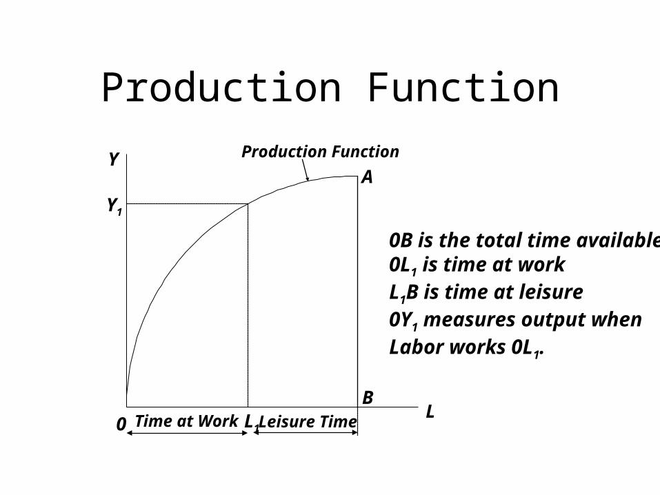
Production Function

L

Y

0 L1

Y1

B

Production Function

Time at Work Leisure Time

A

0B is the total time available0L1 is time at workL1B is time at leisure0Y1 measures output whenLabor works 0L1.

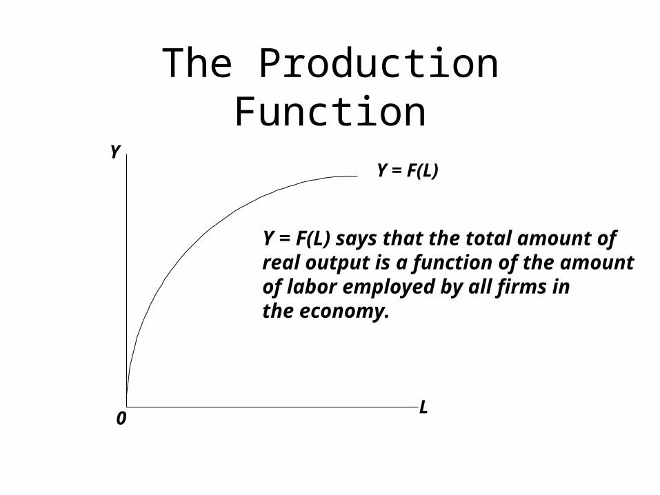
The Production Function

Y = F(L)

L

Y

Y = F(L) says that the total amount of real output is a function of the amount of labor employed by all firms in the economy.

0

The Production Function

• The production function is concave.– This means that the production function’s slope

rises at a decreasing rate.• For every increase in labor, output increases by

smaller amounts.

– The production function is drawn this way because we are assuming the law of diminishing returns causes each additional unit of labor to produce less output.

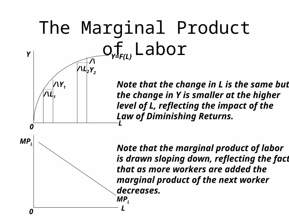
The Marginal Product of Labor

• The slope of the production function is /\Y//\L or the additional amount of output produced when one more worker is added.

• Another name for the change in output divided by the change in labor is the marginal product of labor (MPL).

• Since the production function increases at a decreasing rate, MPL must slope down.

The Marginal Product of Labor

L

L

Y

MPL

Y=F(L)

MPL

/\Y1

/\L1

/\L2

/\Y2

Note that the change in L is the same butthe change in Y is smaller at the higherlevel of L, reflecting the impact of theLaw of Diminishing Returns.

Note that the marginal product of laboris drawn sloping down, reflecting the factthat as more workers are added themarginal product of the next workerdecreases.

0

0

Distribution of Income

• The distribution of national income is determined by factor prices.

• Factor prices are the amounts paid to the factors of production.

• How does a perfectly competitive firm decide how much to pay its factors of production?

Firm Decisions

• A profit-maximizing firm has two decisions to make: How much output to produce and how many workers to hire.– A profit-maximizing perfectly competitive firm

produces output to the point at which its price just equals its marginal cost.

– A profit-maximizing perfectly competitive firm hires factors to the point where the factor’s value of the marginal product just equals its marginal resource cost.

Profits and the Competitive Firm

• A profit maximizing, competitive firm takes the product price and the factor prices as given and chooses the amounts of output, labor and capital that maximize profits.– How does the firm choose?

Profit Maximizing Math: Firm

• Profit = Commodities Supplied – Cost of Labor

• Profit = YS – (w/P)L– The equation shows that profit depends on the

amount of commodities supplied, YS, the product price P, the factor price, w, and the quantity of the factor L.

More Profit Maximizing Math

• Labor Demand– /\Profit = /\Revenue - /\Cost

– /\Profit = (P x MPL) - w = 0

– P x MPL = w

– MPL = w/PLabor Demand

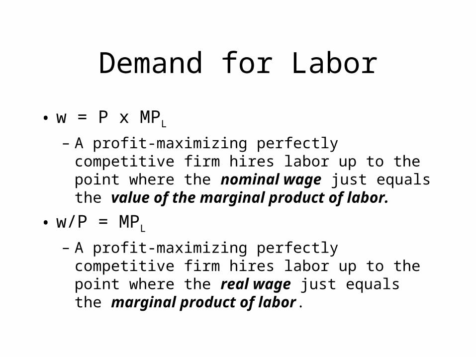
Demand for Labor

• w = P x MPL

– A profit-maximizing perfectly competitive firm hires labor up to the point where the nominal wage just equals the value of the marginal product of labor.

• w/P = MPL

– A profit-maximizing perfectly competitive firm hires labor up to the point where the real wage just equals the marginal product of labor.

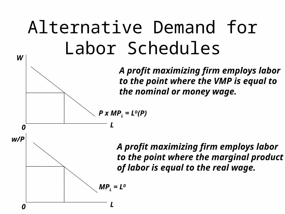
Alternative Demand for Labor Schedules

w/P

W

L

L

MPL = LD

P x MPL = LD(P)

A profit maximizing firm employs laborto the point where the VMP is equal tothe nominal or money wage.

A profit maximizing firm employs laborto the point where the marginal productof labor is equal to the real wage.

0

0

Demand for Labor

• The value of the marginal product of labor schedule for a perfectly competitive firm is that firm’s labor demand schedule.– It shows how many units of labor the firm demands at

any given nominal wage W.

• The marginal product of labor schedule for a perfectly competitive firm is that firm’s labor demand schedule.– It shows how many units of labor the firm demands at

any given real wage W/P.

Nominal Wages and Real Wages?

• The nominal wage is the money wage paid.

• The real wage in the nominal wage adjusted by the price level as measured by the average price of goods and services.– The real wage reflects the true purchasing power of

the worker’s income.

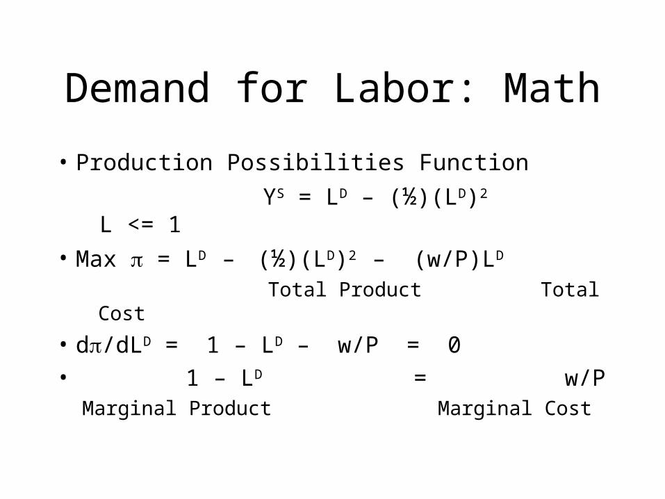
Demand for Labor: Math

• Production Possibilities Function

YS = LD – (½)(LD)2 L <= 1

• Max = LD – (½)(LD)2 – (w/P)LD

Total Product Total Cost

• d/dLD = 1 – LD – w/P = 0

• 1 – LD = w/PMarginal Product Marginal Cost

The Supply of Labor

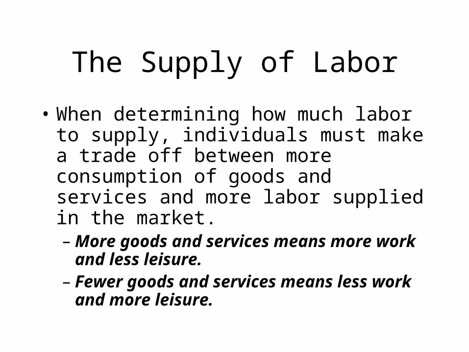
• When determining how much labor to supply, individuals must make a trade off between more consumption of goods and services and more labor supplied in the market.– More goods and services means more work

and less leisure.– Fewer goods and services means less work

and more leisure.

Deriving the Labor Supply

• Demand for Stuff <= Labor Income + Profits

YD <= (w/P)LS + • Deriving Labor Supply:• Utility = Utility of Stuff – Disutility of Working

Max U = (w/P)LS + – (½ LS)2

Stuff Disutility of Working

• Take the first derivative, set to zero, solve for LS

Deriving Labor Supply

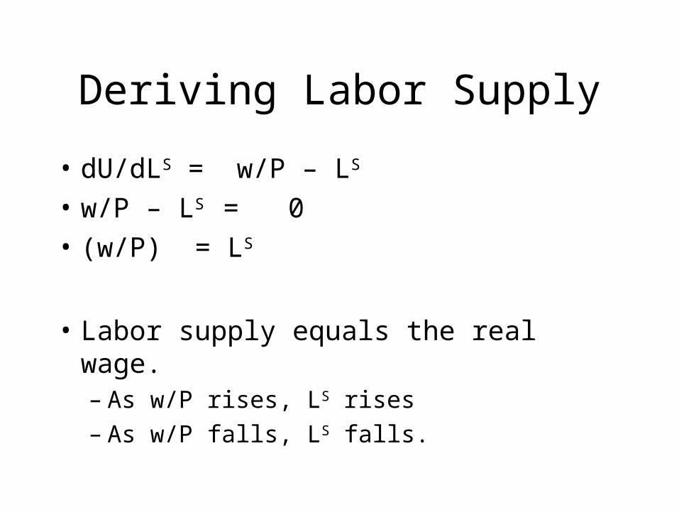
• dU/dLS = w/P – LS

• w/P – LS = 0

• (w/P) = LS

• Labor supply equals the real wage.– As w/P rises, LS rises– As w/P falls, LS falls.

Labor Supply

LS

w/P

0

LS

LS

w/P

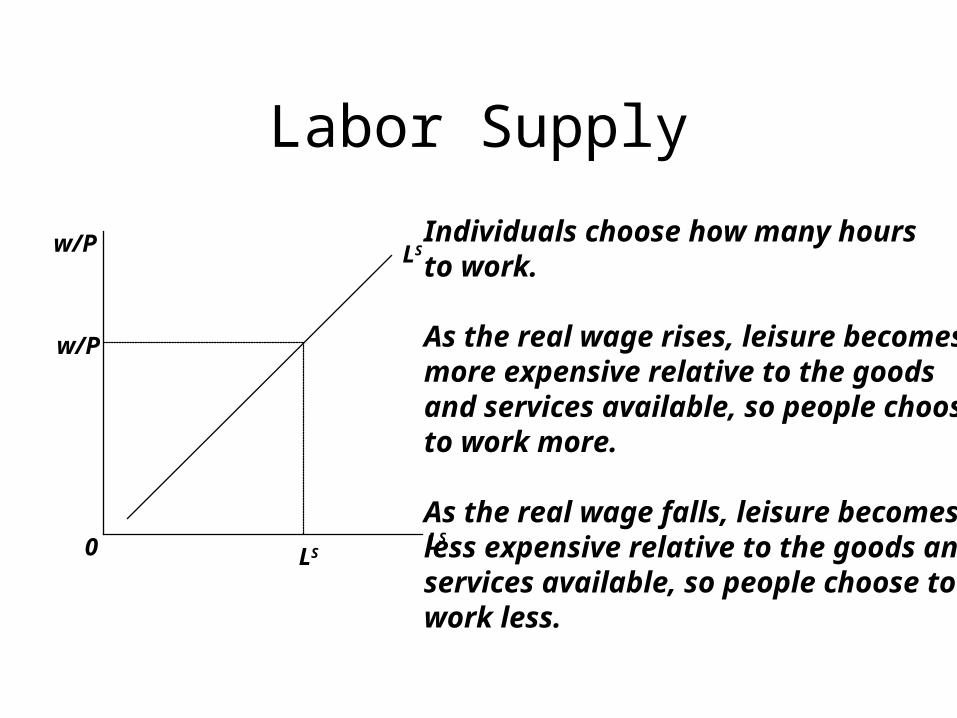
Individuals choose how many hoursto work.

As the real wage rises, leisure becomesmore expensive relative to the goodsand services available, so people chooseto work more.

As the real wage falls, leisure becomesless expensive relative to the goods andservices available, so people choose towork less.

Factors that Shift Labor Supply

• Taxes:– Taxes reduce labor supply by lowering the

wage received by households.• An increase in the tax rate shifts the labor supply

curve to the left.

• A decrease in the tax rate shifts the labor supply curve to the right.

Factors that Shift Labor Supply

• Wealth:– An increase in wealth reduces labor supply by

decreasing the need to work.• An increase in the wealth shifts the labor supply

curve to the left.

• A decrease in the wealth shifts the labor supply curve to the right.

– However, as the USA has become wealthier, labor supply has not decreased. Why?

Labor Supply and Wealth

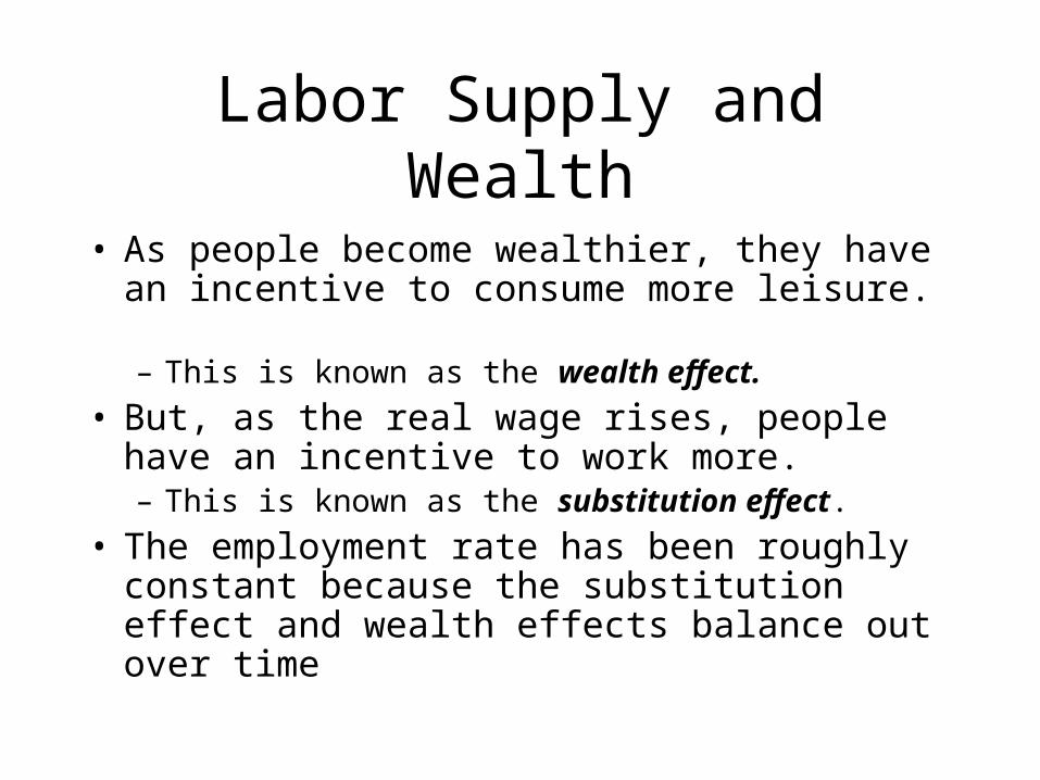
• As people become wealthier, they have an incentive to consume more leisure. – This is known as the wealth effect.

• But, as the real wage rises, people have an incentive to work more. – This is known as the substitution effect.

• The employment rate has been roughly constant because the substitution effect and wealth effects balance out over time

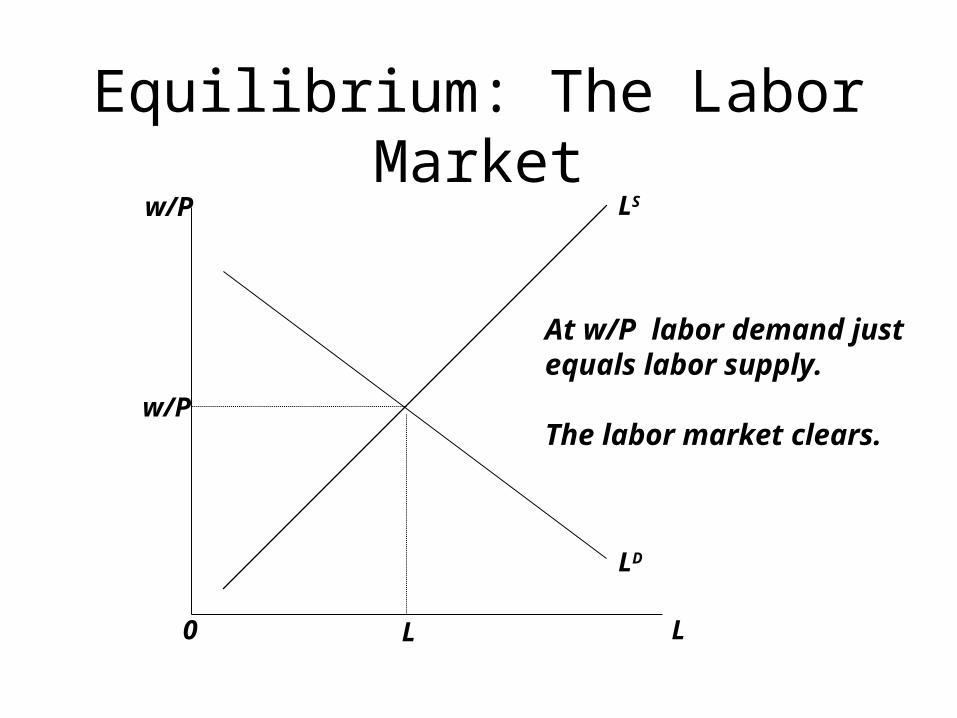
Equilibrium: The Labor Marketw/P

L

LS

At w/P labor demand justequals labor supply.

The labor market clears.

L0

w/P

LD

Putting It All Together

Deriving Aggregate Supply

What Does All This Mean for Aggregate Supply?

• Aggregate supply is the total quantity of goods and services produced by an economy.

• The aggregate supply curve is a schedule relating the total supply of all goods and services in the economy to the general price level.

• What does the aggregate supply curve look like in the classical model?

Y

L

Y

Y

Y

P

L

w/P

Y=F(L)

LS

Production FunctionBalancing Line

Labor MarketAggregate Supply

0

0

0

0

LD

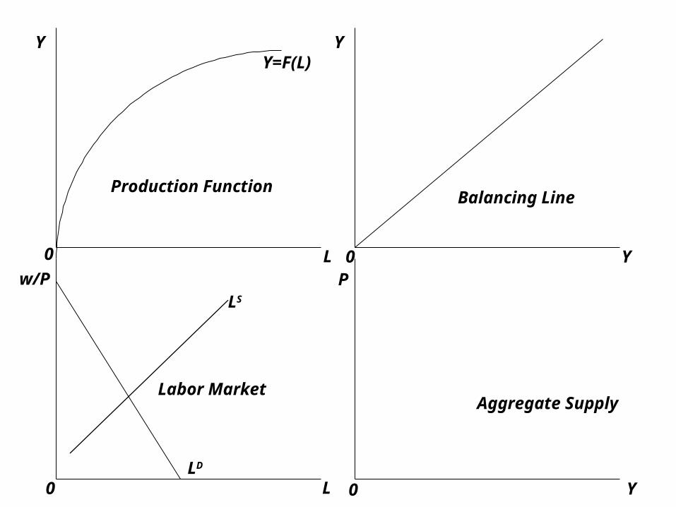
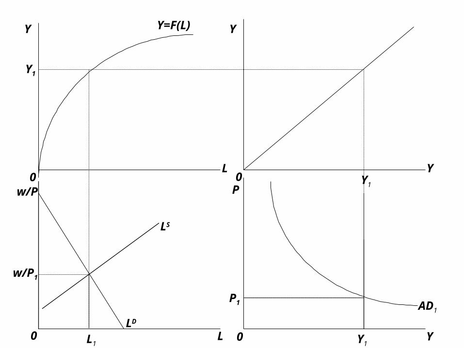
The Model Components

• The production function relates output produced to labor employed.

• Labor employed is determined by labor demand and labor supplied.

• The balancing line transfers output from the vertical axis to the horizontal.

• Aggregate supply will show the relationship between output and the price level.

Y Y

Y

Y

L

P w/PL1

Y1

LS

Y=F(L)

P1

Y1

L1Y1

L0

0

0

0

w/P1.

LD

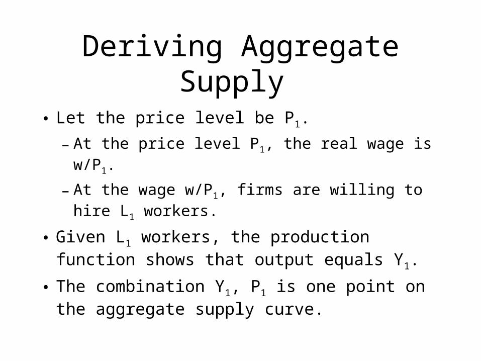
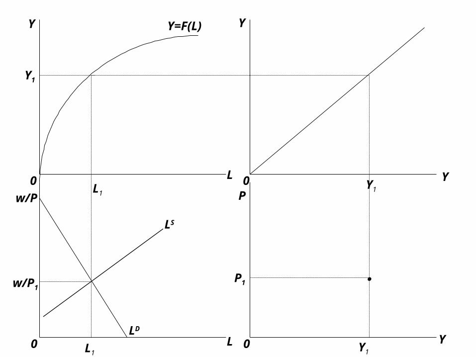
Deriving Aggregate Supply

• Let the price level be P1.

– At the price level P1, the real wage is w/P1.

– At the wage w/P1, firms are willing to hire L1 workers.

• Given L1 workers, the production function shows that output equals Y1.

• The combination Y1, P1 is one point on the aggregate supply curve.

Y Y

Y

Y

L

P w/P

Y1

LS

w/P1

Y=F(L)

P1

Y1

LS Y1L

P2

0

0

0

0

w/P2

LD

AS

.

.

LD

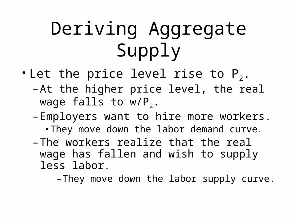
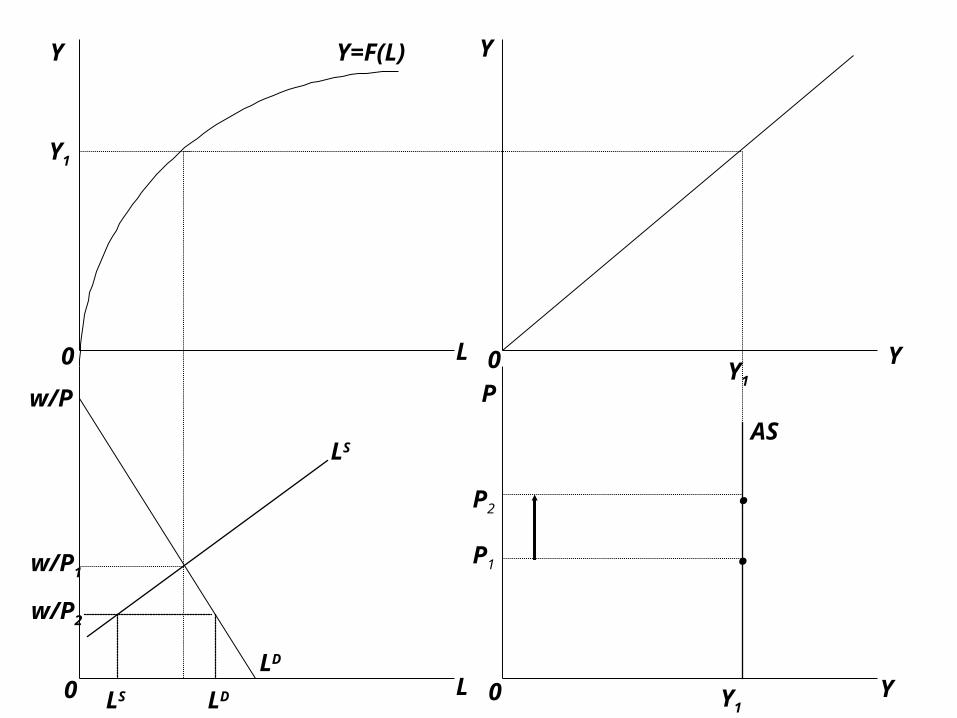
Deriving Aggregate Supply

• Let the price level rise to P2.– At the higher price level, the real wage falls

to w/P2.– Employers want to hire more workers.

• They move down the labor demand curve.

– The workers realize that the real wage has fallen and wish to supply less labor.

– They move down the labor supply curve.

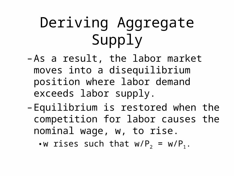
Deriving Aggregate Supply

– As a result, the labor market moves into a disequilibrium position where labor demand exceeds labor supply.

– Equilibrium is restored when the competition for labor causes the nominal wage, w, to rise.• w rises such that w/P2 = w/P1.

Classical Aggregate Supply

• At the new equilibrium, the price level is P2 and output is still Y1. This combination is another point on the aggregate supply curve.– The aggregate supply curve is vertical at the full

employment level of output because the level of employment of labor does not change as the price level changes.

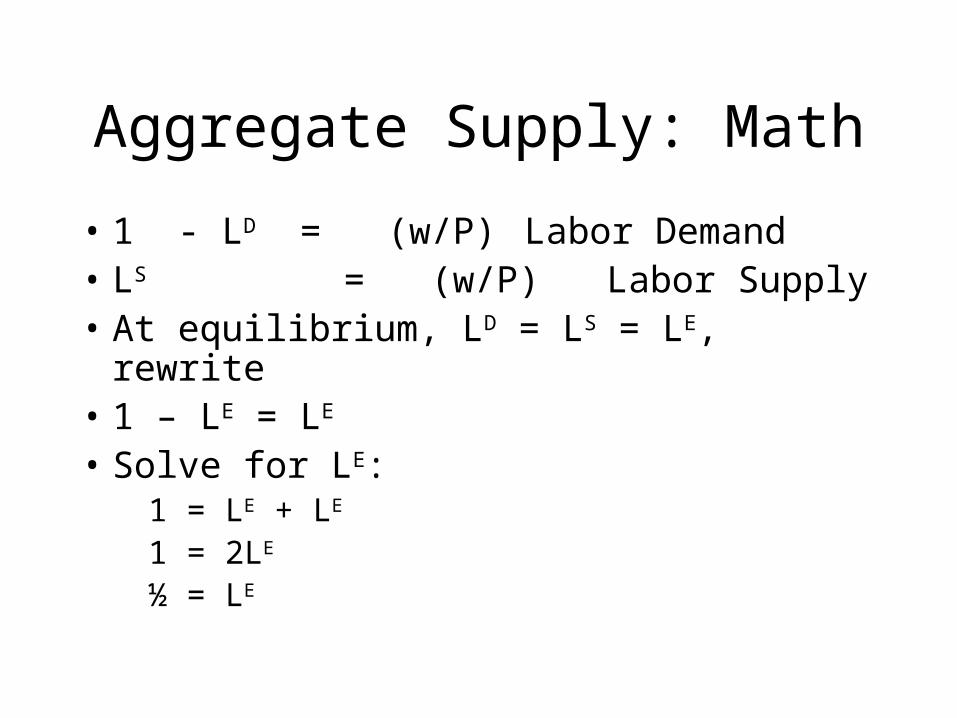
Aggregate Supply: Math

• 1 - LD = (w/P)Labor Demand• LS = (w/P)Labor Supply• At equilibrium, LD = LS = LE, rewrite• 1 – LE = LE • Solve for LE:

1 = LE + LE

1 = 2LE

½ = LE

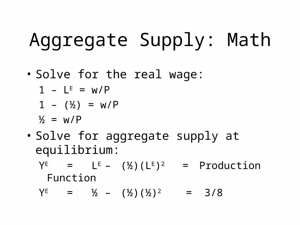
Aggregate Supply: Math

• Solve for the real wage:1 – LE = w/P

1 – (½) = w/P

½ = w/P

• Solve for aggregate supply at equilibrium:YE = LE – (½)(LE)2 = Production Function

YE = ½ – (½)(½)2 = 3/8

Models Answer Questions

• What will happen to output in this model if labor productivity increases or decreases?

• What will happen to output if labor resources increase or decrease?

Business Fluctuations

• According to the classical theory of employment and GDP, the explanation of business fluctuations lies with the factors that determine equilibrium in the labor market. They are:– Preferences– Endowments– Technology

Preferences, Endowments, Technology

• Factors that cause fluctuations in the level of output are those that shift labor demand and labor supply.– Labor demand shifts with changes in

technology and resource endowment– Labor supply shifts with changes in

preferences.

Y

L

Y

Y

Y

Pw/P

Y1=F(L)

LS

L1

Y1

Y1L

w1/P1

0

0

0

0

Y2=F(L)Y2

Y2

AS1AS2

1

2

1

2

w2/P1

LD1

LD2

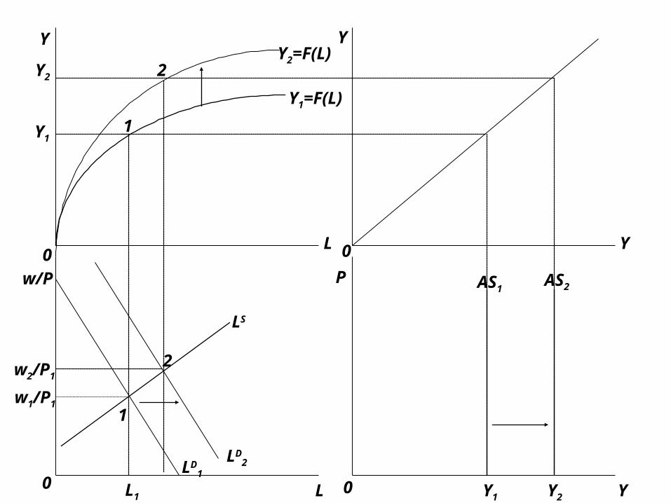
Change in Technology

• New technology increases productivity.– The production function shifts up.– The labor demand curve shifts to the right.

• The increase in demand for labor increases the real wage, causing an increase in labor supply along the labor supply curve.

• Aggregate supply increases.– At the price level, P1, more output is produced.

Increase in Aggregate Supply

• Aggregate supply increases for two reasons:– The higher real wage increased the number of

laborers in the labor supply.– The new technology increased the productivity

of each worker.

Resource Endowment

• An increase in resource endowment has the same impact as an improvement in technology, if it caused an increase in labor productivity.

Y Y

Y

Y

L

P w/P

Y1

LS1

Y=F(L)

Y1

L1 L2Y1 Y2

L0

0

0

0

w1/P1

LS2

Y2

w2/P1

LD

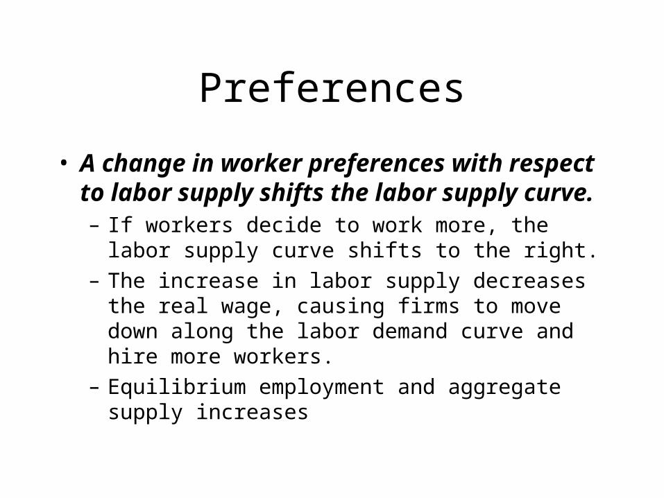
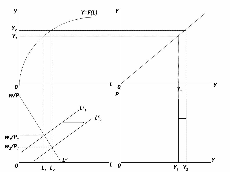
Preferences

• A change in worker preferences with respect to labor supply shifts the labor supply curve.– If workers decide to work more, the labor supply curve

shifts to the right.

– The increase in labor supply decreases the real wage, causing firms to move down along the labor demand curve and hire more workers.

– Equilibrium employment and aggregate supply increases

Y

L

Y

Y

Y

P

L

w/P

Y=F(L)

LS

P1

L1

Y1

Y1

Y1

AD1

w/P1

0

0 0

0LD