The Theory of Consumer Behavior

ZURONI MD JUSOH

DEPT OF RESOURCE MANAGEMENT & CONSUMER STUDIES

FACULTY OF HUMAN ECOLOGY

UPM

The Theory of Consumer Behavior

The principle assumption upon which the theory of consumer behavior and demand is built is: a consumer attempts to allocate his/her limited money income among available goods and services so as to maximize his/her utility (satisfaction).

Theory of Consumer Behavior

Useful for understanding the demand side of the market.

Utility - amount of satisfaction derived from the consumption of a commodity ….measurement units utils

Theories of Consumer Choice

Utility Concepts:

– The Cardinal Utility Theory (TUC)

• Utility is measurable in a cardinal sense

• cardinal utility - assumes that we can assign values for utility, (Jevons, Walras, and Marshall). E.g., derive 100 utils from eating a slice of pizza

– The Ordinal Utility Theory (TUO)

• Utility is measurable in an ordinal sense

• ordinal utility approach - does not assign values, instead works with a ranking of preferences. (Pareto, Hicks, Slutsky)

The Cardinal Approach

Nineteenth century economists, such as Jevons, Menger and Walras, assumed that utility was measurable in a cardinal sense, which means that the difference between two measurement is itself numerically significant.

UX = f (X), UY = f (Y), …..

Utility is maximized when:

MUX / MUY = PX / PY

The Cardinal Approach

Total utility (TU) - the overall level of satisfaction derived from consuming a good or service

Marginal utility (MU) additional satisfactionthat an individual derives from consuming an additional unit of a good or service.Formula :

MU = Change in total utility

Change in quantity

= ∆ TU

∆ Q

The Cardinal Approach

Law of Diminishing Marginal Utility (Return) = As more and more of a good are consumed, the process of consumption will (at some point) yield smaller and smaller additions to utility

When the total utility maximum, marginal utility = 0

When the total utility begins to decrease, the marginal utility = negative (-ve)

EXAMPLE

Number Purchased

Total Utility

Marginal Utility

0 0 0

1 4 4

2 7 3

3 8 1

4 8 0

5 7 -1

The Cardinal Approach

TU, in general, increases with Q

At some point, TU can start falling with Q (see Q = 5)

If TU is increasing, MU > 0

From Q = 1 onwards, MU is declining principle of diminishing marginal utility As more and more of a good are consumed, the process of consumption will (at some point) yield smaller and smaller additions to utility

Consumer Equilibrium

So far, we have assumed that any amount of goods and services are always available for consumption

In reality, consumers face constraints (income and prices):

– Limited consumers income or budget

– Goods can be obtained at a price

Some simplifying assumptions

Consumer’s objective: to maximize his/her utility subject to income constraint

2 goods (X, Y)

Prices Px, Py are fixed

Consumer’s income (I) is given

Consumer Equilibrium

Marginal utility per price additional utility derived from spending the next price (RM) on the good

MU per RM = MU

P

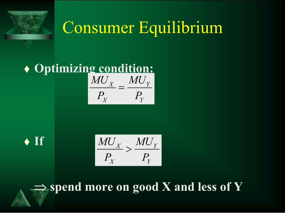
Consumer Equilibrium

Optimizing condition:

If

spend more on good X and less of Y

X Y

X Y

MU MU

P P

X Y

X Y

MU MU

P P

Numerical Illustration

Qx TUX MUX MUxPx

QY TUY MUY MUyPy

1 30 30 15 1 50 50 5

2 39 9 4.5 2 105 55 5.5

3 45 6 3 3 148 43 4.3

4 50 5 2.5 4 178 30 3

5 54 4 2 5 198 20 2

6 56 2 1 6 213 15 1.5

Simple Illustration

Suppose: X = fishball Y = fishcake

Assume: PX = 2PY = 10

Cont.

2 potential optimum positions

Combination A: X = 3 and Y = 4

– TU = TUX + TUY = 45 + 178 = 223

Combination B: X = 5 and Y = 5

– TU = TUX + TUY = 54 + 198 = 252

Cont.

Presence of 2 potential equilibrium positions suggests that we need to consider income. To do so let us examine how much each consumer spends for each combination.

Expenditure per combination

– Total expenditure = PX X + PY Y

– Combination A: 3(2) + 4(10) = 46

– Combination B: 5(2) + 5(10) = 60

Cont.

Scenarios:

– If consumer’s income = 46, then the optimum is given by combination A. .…Combination B is not affordable

– If the consumer’s income = 60, then the optimum is given by Combination B….Combination A is affordable but it yields a lower level of utility

The Ordinal Approach

Economists following the lead of Hicks, Slutsky and Pareto believe that utility is measurable in an ordinal sense--the utility derived from consuming a good, such as X, is a function of the quantities of X and Y consumed by a consumer.

U = f ( X, Y )

Cont.

Ordinal Utility Theory (TUO)

– Can be measured in qualitative, not quantitative, but only lists the main options (indifference curves & budget line).

Rational human beings will choose to maximize the utility by selecting the highest utility

Difference consumers, difference utilities.

INDIFFERENCE CURVE (IC)

Curve where the points represent a combination of items when the consumer at indifference situation (satisfaction).

Axes: both axes refer to the quantity of goods

For the combination that produces a higher level of satisfaction, the curves shift to the right (IC2) from the first curve (IC1)

In contrast, the curves shift to the left (IC-1)

INDIFFERENCE CURVE

Y

O

goods

7

Y

O

X

IC2

IC1

M

IC-1

114

goods

SA

B

C

DT

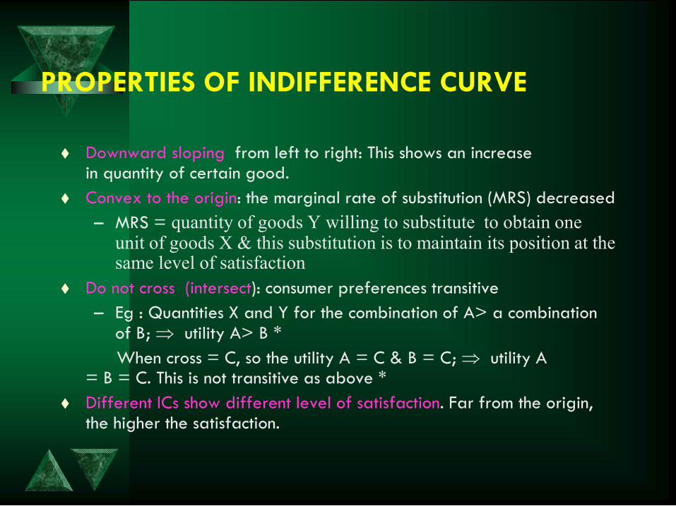
PROPERTIES OF INDIFFERENCE CURVE

Downward sloping from left to right: This shows an increase in quantity of certain good.

Convex to the origin: the marginal rate of substitution (MRS) decreased

– MRS = quantity of goods Y willing to substitute to obtain one unit of goods X & this substitution is to maintain its position at the same level of satisfaction

Do not cross (intersect): consumer preferences transitive

– Eg : Quantities X and Y for the combination of A> a combination of B; utility A> B *

When cross = C, so the utility A = C & B = C; utility A = B = C. This is not transitive as above *

Different ICs show different level of satisfaction. Far from the origin, the higher the satisfaction.

IC curves can not intersect

Good Y

C A IC1

B

IC2

Good X

Budget line (BL)

Line showing all combinations of items can be purchased for a particular level of income (M) ;

M =PxQx + PyQy

The slope depends on the prices of goods X and Y, the slope = Px/Py

Slope -ve: to use more goods X, Y should reduce & vice versa

In the X-axis, when the quantity Y = 0, all M used to purchase X; M = PxQx Qx =M/Px

At the Y axis, when the quantity X = 0, all M used to purchase Y; M = PyQy Qy =M/Py

FACTORS SHIFT THE BUDGET LINE

Changes in prices of goods X

Y

Px Px X

EFFECTS OF PRICE CHANGES ON THE BUDGET LINE

When price of good X increases, the quantity of good X is reduced (by maintaining the quantity of Y) & vice versa.

Points on the X axis shifted to the left (a small quantity of X)

When the price of Y increases, the quantity Y is reduced (by maintaining the quantity of X) & vice versa

Point on Y axis move to the bottom (small quantity in Y)

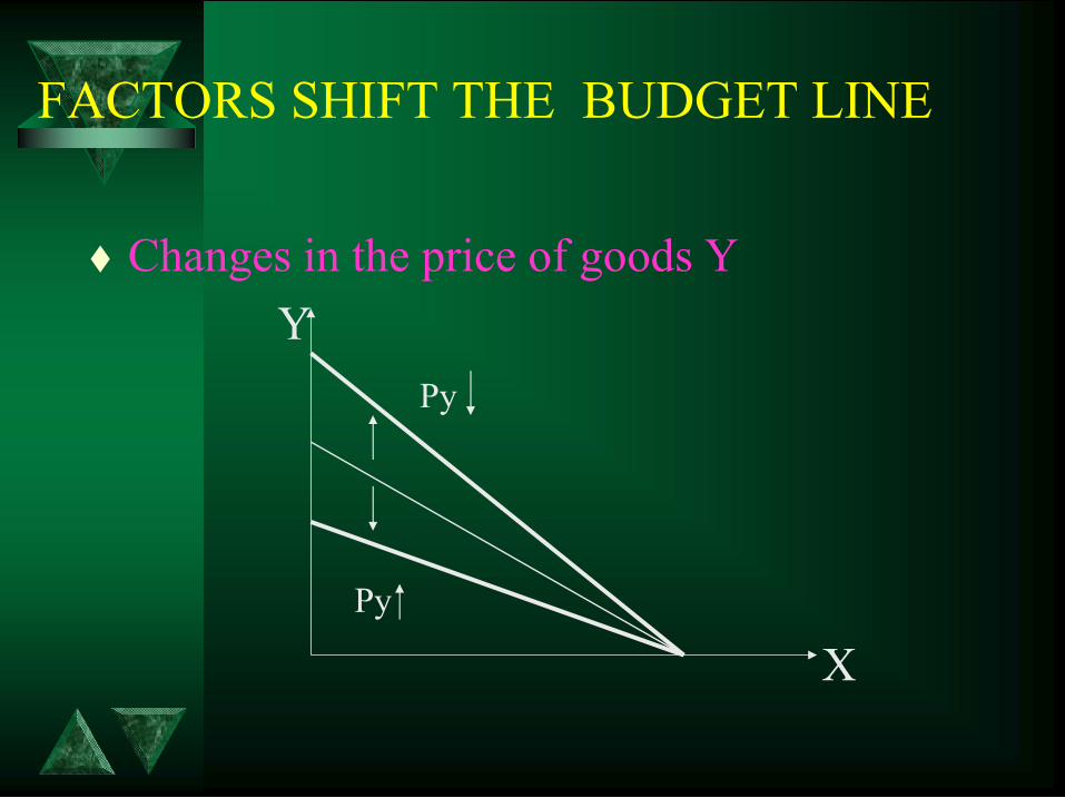
FACTORS SHIFT THE BUDGET LINE

Changes in the price of goods Y

Y

Py

Py

X

FACTORS SHIFT THE BUDGET LINE

Changes in income

Y

I

I

X

EFFECTS OF INCOME CHANGES ON THE BUDGET LINE

When M increases, QX and QY can be bought even more, a point on the X axis shifted to the right & a point on the Y axis move on; & vice versa when M decreases.

CONSUMER EQUILIBRIUM

With income (M) some combination of goods that consumers choose the highest satisfaction

Satisfied the same curves and budget lines are connected

The point where the curve IC and BL tangent

Slope IC = BL

Consumer choice influenced by income

Increased income, increased consumer equilibrium point

MAXIMIZE CONSUMER SATISFACTION

F

E

B

A D

C

Y

OX

IC1

IC2

IC3

IC4

M1

M

Budget line (BL)

Indifference Curves (IC)

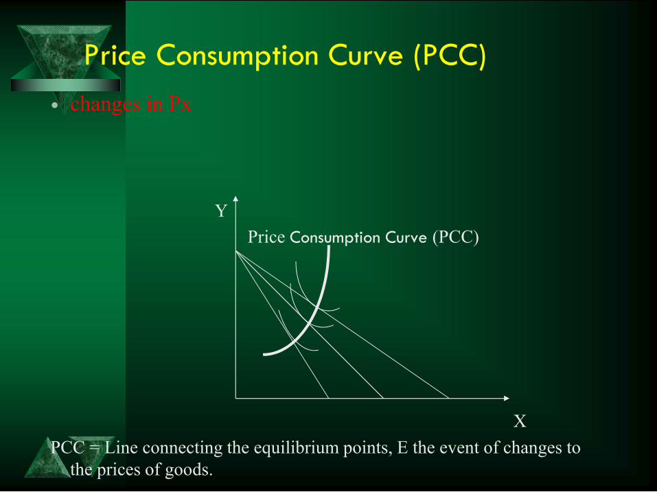
Price Consumption Curve (PCC)

changes in Px

Y

Price Consumption Curve (PCC)

X

PCC = Line connecting the equilibrium points, E the event of changes to the prices of goods.

Formation of Demand Curve

Outcome of PCC

Px

Dd

Qty X

Demand Curve for Normal Goods and Inferior Goods

X axis, Y axis of the quantity of goods, the price of goods

Px

Normal goods

Inferior goodsQty X

Normal goods= P , Dd

Inferior goods= P , Dd

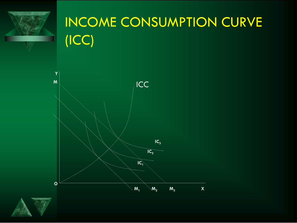
INCOME CONSUMPTION CURVE (ICC)

If a fixed price and income increases, the budget line shifts to the right, thus shifting the equilibrium point higher.

Equilibrium point some income items associated with the line - can be income consumption curve (ICC).

ICC shows the points for the combination of goods that can be purchased when income change and fixed in price.

INCOME CONSUMPTION CURVE (ICC)

Y

OX

IC3

IC2

M3

M

IC1

M2M1

ICC

ENGEL CURVE

OX20

M

1612 22

40

Engel curve for x

20

10

30

ENGEL CURVE

Relationship of income to the quantity of an item

Retrieved from ICC

Get a quantity of goods X or Y that can be purchased goods with an income

Plot the quantity of X or Y against income

Linking income changes with changes in demand for goods at a fixed price

Engel curve for luxury goods and normal goods

M

X

Normal goods

Luxury goods

O

Conclusion

ToCB showing how it provides users a combination of sources of income for many goods /services

There are two types of utility theory:

– Cardinal TU and MU

– Ordinal curve IC and BL

Equilibrium and utility maximization can be either TUC or TUO

Equilibrium points of connection to produce PCC (change IN PRICE) and ICC (change in income)

Displaying Publication = PCC curve DD & ICC = Engel curve (EC)

The types of goods obtained displaying income or price changes.

Thank You