Embed Size (px)
Citation preview
The Theory of Measures and
Integration
A Solution Manual for Vestrup (2003)
Jianfei Shen
School of Economics, The University of New South Wales
Sydney, Australia

I hear, I forget;I see, I remember;I do, I understand.
Old Proverb

Contents
Preface . . . . . . . . . . . . . . . . . . . . . . . . . . . . . . . . . . . . . . . . . . . . . . . . . . . . . . . . . . . . . . . . ix
Acknowledgements . . . . . . . . . . . . . . . . . . . . . . . . . . . . . . . . . . . . . . . . . . . . . . . . . . . . xi
1 Set Systems . . . . . . . . . . . . . . . . . . . . . . . . . . . . . . . . . . . . . . . . . . . . . . . . . . . . . . . 1
1.1 �-Systems, �-Systems, and Semirings . . . . . . . . . . . . . . . . . . . . . . . . . . 2
1.1.1 �-Systems . . . . . . . . . . . . . . . . . . . . . . . . . . . . . . . . . . . . . . . . . . . . . . 2
1.1.2 �-System . . . . . . . . . . . . . . . . . . . . . . . . . . . . . . . . . . . . . . . . . . . . . . . 4
1.1.3 Semiring . . . . . . . . . . . . . . . . . . . . . . . . . . . . . . . . . . . . . . . . . . . . . . . . 6
1.2 Fields . . . . . . . . . . . . . . . . . . . . . . . . . . . . . . . . . . . . . . . . . . . . . . . . . . . . . . . . . 15
1.3 � -Fields . . . . . . . . . . . . . . . . . . . . . . . . . . . . . . . . . . . . . . . . . . . . . . . . . . . . . . . 21
1.4 The Borel � -Field . . . . . . . . . . . . . . . . . . . . . . . . . . . . . . . . . . . . . . . . . . . . . . 28
2 Measures . . . . . . . . . . . . . . . . . . . . . . . . . . . . . . . . . . . . . . . . . . . . . . . . . . . . . . . . . . 29
2.1 Measures . . . . . . . . . . . . . . . . . . . . . . . . . . . . . . . . . . . . . . . . . . . . . . . . . . . . . 30
2.2 Continuity of Measures . . . . . . . . . . . . . . . . . . . . . . . . . . . . . . . . . . . . . . . . 35
2.3 A Class of Measures . . . . . . . . . . . . . . . . . . . . . . . . . . . . . . . . . . . . . . . . . . . 47
3 Extensions of Measures . . . . . . . . . . . . . . . . . . . . . . . . . . . . . . . . . . . . . . . . . . . . 53
3.1 Extensions and Restrictions . . . . . . . . . . . . . . . . . . . . . . . . . . . . . . . . . . . . 54
3.2 Outer Measures . . . . . . . . . . . . . . . . . . . . . . . . . . . . . . . . . . . . . . . . . . . . . . . 55
3.3 Carathéodory’s Criterion . . . . . . . . . . . . . . . . . . . . . . . . . . . . . . . . . . . . . . 57
3.4 Existence of Extensions . . . . . . . . . . . . . . . . . . . . . . . . . . . . . . . . . . . . . . . . 60
3.5 Uniqueness of Measures and Extensions . . . . . . . . . . . . . . . . . . . . . . . . 63
3.6 The Completion Theorem . . . . . . . . . . . . . . . . . . . . . . . . . . . . . . . . . . . . . . 66
3.7 The Relationship between �.A/ and M.��/ . . . . . . . . . . . . . . . . . . . . . 67
3.8 Approximations . . . . . . . . . . . . . . . . . . . . . . . . . . . . . . . . . . . . . . . . . . . . . . . 68
3.9 A Further Description of M.��/ . . . . . . . . . . . . . . . . . . . . . . . . . . . . . . . . 68
4 Lebesgue Measure . . . . . . . . . . . . . . . . . . . . . . . . . . . . . . . . . . . . . . . . . . . . . . . . . 71
4.1 Lebesgue Measure: Existence and Uniqueness . . . . . . . . . . . . . . . . . . . 71
4.2 Lebesgue Sets . . . . . . . . . . . . . . . . . . . . . . . . . . . . . . . . . . . . . . . . . . . . . . . . . 73
4.3 Translation Invariance of Lebesgue Measure . . . . . . . . . . . . . . . . . . . . 73
v
vi CONTENTS
5 Measurable Functions . . . . . . . . . . . . . . . . . . . . . . . . . . . . . . . . . . . . . . . . . . . . . 77
5.1 Measurability . . . . . . . . . . . . . . . . . . . . . . . . . . . . . . . . . . . . . . . . . . . . . . . . . 77
5.2 Combining Measurable Functions . . . . . . . . . . . . . . . . . . . . . . . . . . . . . . 79
5.3 Sequences of Measurable Functions . . . . . . . . . . . . . . . . . . . . . . . . . . . . 83
5.4 Almost Everywhere . . . . . . . . . . . . . . . . . . . . . . . . . . . . . . . . . . . . . . . . . . . . 84
5.5 Simple Functions . . . . . . . . . . . . . . . . . . . . . . . . . . . . . . . . . . . . . . . . . . . . . . 84
5.6 Some Convergence Concepts . . . . . . . . . . . . . . . . . . . . . . . . . . . . . . . . . . . 86
5.7 Continuity and Measurability . . . . . . . . . . . . . . . . . . . . . . . . . . . . . . . . . . 90
5.8 A Generalized Definition of Measurability . . . . . . . . . . . . . . . . . . . . . . 90
6 The Lebesgue Integral . . . . . . . . . . . . . . . . . . . . . . . . . . . . . . . . . . . . . . . . . . . . . 93
6.1 Stage One: Simple Functions . . . . . . . . . . . . . . . . . . . . . . . . . . . . . . . . . . . 93
6.2 Stage Two: Nonnegative Functions . . . . . . . . . . . . . . . . . . . . . . . . . . . . . 96
6.3 Stage Three: General Measurable Functions . . . . . . . . . . . . . . . . . . . . . 104
6.4 Stage Four: Almost Everywhere Defined Functions . . . . . . . . . . . . . . 109
7 Integrals Relative to Lebesgue Measure . . . . . . . . . . . . . . . . . . . . . . . . . . . . 111
7.1 Semicontinuity . . . . . . . . . . . . . . . . . . . . . . . . . . . . . . . . . . . . . . . . . . . . . . . . 111
8 The Lp Spaces . . . . . . . . . . . . . . . . . . . . . . . . . . . . . . . . . . . . . . . . . . . . . . . . . . . . 113
8.1 Lp Space: The Case 1 6 p < C1 . . . . . . . . . . . . . . . . . . . . . . . . . . . . . . . 113
8.2 The Riesz-Fischer Theorem . . . . . . . . . . . . . . . . . . . . . . . . . . . . . . . . . . . . 117
8.3 Lp Space: The Case 0 < p < 1 . . . . . . . . . . . . . . . . . . . . . . . . . . . . . . . . . . 119
8.4 Lp Space: The Case p D C1 . . . . . . . . . . . . . . . . . . . . . . . . . . . . . . . . . . . 123
8.5 Containment Relations for Lp Spaces . . . . . . . . . . . . . . . . . . . . . . . . . . 125
8.6 Approximation . . . . . . . . . . . . . . . . . . . . . . . . . . . . . . . . . . . . . . . . . . . . . . . . 127
8.7 More Convergence Concepts . . . . . . . . . . . . . . . . . . . . . . . . . . . . . . . . . . . 127
8.8 Prelude to the Riesz Representation Theorem . . . . . . . . . . . . . . . . . . 129
9 The Radon-Nikodym Theorem . . . . . . . . . . . . . . . . . . . . . . . . . . . . . . . . . . . . . 131
9.1 The Radon-Nikodym Theorem, Part I . . . . . . . . . . . . . . . . . . . . . . . . . . . 131
10 Products of Two Measure Spaces . . . . . . . . . . . . . . . . . . . . . . . . . . . . . . . . . . 139
10.1 Product Measures . . . . . . . . . . . . . . . . . . . . . . . . . . . . . . . . . . . . . . . . . . . . . 139
10.2 The Fubini Theorems . . . . . . . . . . . . . . . . . . . . . . . . . . . . . . . . . . . . . . . . . . 143
11 Arbitrary Products of Measure Spaces . . . . . . . . . . . . . . . . . . . . . . . . . . . . . 145
11.1 Notation and Conventions . . . . . . . . . . . . . . . . . . . . . . . . . . . . . . . . . . . . . 145
11.2 Construction of the Product Measure . . . . . . . . . . . . . . . . . . . . . . . . . . . 147
References . . . . . . . . . . . . . . . . . . . . . . . . . . . . . . . . . . . . . . . . . . . . . . . . . . . . . . . . . . . . 155
List of Figures
1.1 Inclusion between classes of sets A � 2˝ . . . . . . . . . . . . . . . . . . . . . . . . 1
3.1 A [ B 2M.�/ . . . . . . . . . . . . . . . . . . . . . . . . . . . . . . . . . . . . . . . . . . . . . . . . . . . 57
6.1 f1 and f2. . . . . . . . . . . . . . . . . . . . . . . . . . . . . . . . . . . . . . . . . . . . . . . . . . . . . . . 107
6.2 fn ! f . . . . . . . . . . . . . . . . . . . . . . . . . . . . . . . . . . . . . . . . . . . . . . . . . . . . . . . . . 107
8.1 f p and f q . . . . . . . . . . . . . . . . . . . . . . . . . . . . . . . . . . . . . . . . . . . . . . . . . . . . . . 126
8.2 fn��! 0, but fn 6
Lp
��! 0. . . . . . . . . . . . . . . . . . . . . . . . . . . . . . . . . . . . . . . . . . . . . 128
8.3 . . . . . . . . . . . . . . . . . . . . . . . . . . . . . . . . . . . . . . . . . . . . . . . . . . . . . . . . . . . . . . . . 130
vii


Preface
Sydney, Jianfei Shen
ix

Acknowledgements
xi

1SET SYSTEMS
Remarks
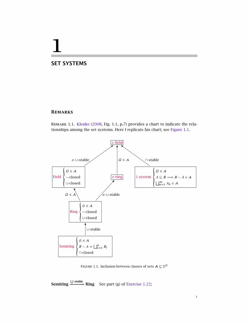
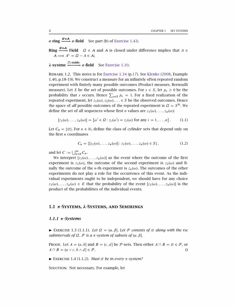
Remark 1.1. Klenke (2008, Fig. 1.1, p.7) provides a chart to indicate the rela-
tionships among the set systems. Here I replicate his chart; see Figure 1.1.
� -field
� -ring
Ring
‚¿ 2 A
X-closed
[-closed
Semiring
‚¿ 2 A
B X A DFniD1 Bi
\-closed
Field
‚˝ 2 A
X-closed
[-closed
�-system
‚˝ 2 A
A � B H) B X A 2 AF1nD1 An 2 A
� -[-stable ˝ 2 A \-stable
˝ 2 A � -[-stable
[-stable
Figure 1.1. Inclusion between classes of sets A � 2˝
SemiringS
-stable������! Ring See part (g) of Exercise 1.22;
1
2 CHAPTER 1 SET SYSTEMS
� -ring˝2A����! � -field See part (b) of Exercise 1.43;
Ring˝2A����! Field ˝ 2 A and A is closed under difference implies that A 2
A H) Ac D ˝ � A 2 A;
�-systmeT
-stable������! � -field See Exercise 1.10.
Remark 1.2. This notes is for Exercise 1.34 (p.17). See Klenke (2008, Example
1.40, p.18-19). We construct a measure for an infinitely often repeated random
experiment with finitely many possible outcomes (Product measure, Bernoulli
measure). Let S be the set of possible outcomes. For s 2 S , let ps > 0 be the
probability that s occurs. HencePs2S ps D 1. For a fixed realization of the
repeated experiment, let z1.!/; z2.!/; : : : 2 S be the observed outcomes. Hence
the space of all possible outcomes of the repeated experiment is ˝ D SN. We
define the set of all sequences whose first n values are z1.!/; : : : ; zn.!/:
Œz1.!/; : : : ; zn.!/� D˚!0 2 ˝ W zi .!
0/ D zi .!/ for any i D 1; : : : ; n: (1.1)
Let C0 D f¿g. For n 2 N, define the class of cylinder sets that depend only on
the first n coordinates
Cn D fŒz1.!/; : : : ; zn.!/� W z1.!/; : : : ; zn.!/ 2 Sg ; (1.2)
and let C ´S1nD0 Cn.
We interpret Œz1.!/; : : : ; zn.!/� as the event where the outcome of the first
experiment is z1.!/, the outcome of the second experiment is z2.!/ and fi-
nally the outcome of the n-th experiment is zn.!/. The outcomes of the other
experiments do not play a role for the occurrence of this event. As the indi-
vidual experiments ought to be independent, we should have for any choice
z1.!/; : : : ; zn.!/ 2 E that the probability of the event Œz1.!/; : : : ; zn.!/� is the
product of the probabilities of the individual events.
1.1 �-Systems, �-Systems, and Semirings
1.1.1 �-Systems
I Exercise 1.3 (1.1.1). Let ˝ D .˛; ˇ�. Let P consists of ¿ along with the rsc
subintervals of ˝. P is a �-system of subsets of .˛; ˇ�.
Proof. Let A D .a; b� and B D .c; d � be P -sets. Then either A \ B D ¿ 2 P , or
A \ B D .a _ c; b ^ d� 2 P . ut
I Exercise 1.4 (1.1.2). Must ¿ be in every �-system?
Solution. Not necessary. For example, let
SECTION 1.1 �-SYSTEMS, �-SYSTEMS, AND SEMIRINGS 3
˝ D .0; 1�; A D .0; 1=2�; B D .1=4; 1�; C D .1=4; 1=2�;
and let P D fA;B;C g. Then P is a �-system on ˝, and ¿ … P . Generally, if
A \ B ¤ ¿ for any A;B in a �-system, then ¿ does not in this �-system. ut
I Exercise 1.5 (1.1.3). List all �-systems consisting of at least two subsets of
f!1; !2; !3g.
Solution. These �-systems are:
�˚f!ig; f!i ; !j g
, .i; j / 2 f1; 2; 3g2 and j ¤ i ;
�˚f!ig; f!1; !2; !3g
;
�˚f!i ; !j g; f!1; !2; !3g
;
�˚f!ig; f!i ; !j g; f!1; !2; !3g
;
�˚¿; f!ig; f!i ; !j g
, i D 1; 2; 3, and j ¤ i ;
�˚¿; f!i ; !j g; f!1; !2; !3g
;
�˚¿; f!ig; f!i ; !j g; f!1; !2; !3g
. ut
I Exercise 1.6 (1.1.4). If Pk consists of the empty set and the k-dimensional
rectangles of any one form, then Pk is a �-system of subsets of Rk .
Proof. Let A;B 2 Pk be two k-dimensional rectangles of any form. We also
write A D A1 � A2 � � � � � Ak and B D B1 � � � � � Bk , where Ai and Bi are rsc
intervals for every i 2 f1; : : : ; ng. We also assume that A ¤ ¿ and B ¤ ¿; for
otherwise A \B D ¿ 2 Pk is trivial. Then
A \B D .A1 � � � � � Ak/ \ .B1 � � � � � Bk/ Dk
�iD1
.Ai \ Bi / 2 Pk
since Ai \ Bi is a rsc interval in R. ut
I Exercise 1.7 (1.1.5). Let P consist of ¿ and all subsets of Rk that are neither
open nor closed. Then P is not a �-system of subsets of Rk .
Proof. To get some intuition, let k D 1. Consider two P -sets: A D .0; 1=2�
and B D Œ1=4; 1/. Note that neither A nor B are open or closed on R, but their
intersection A \ B D Œ1=4; 1=2� is closed on R, and is not in P .
Now consider the k-dimensional case. Let A;B 2 P ; let A D�kiD1Ai and
B D�kiD1 Bi ; particularly, we let Ai D .ai ; bi � and Bi D Œci ; di /, where ai < ci <
bi < di . Then .ai ; bi � \ Œci ; di / D Œci ; bi � ¤ ¿, and A \ B D�kiD1 .Ai \ Bi / D
�kiD1 Œci ; bi � is closed on Rk . ut
I Exercise 1.8 (1.1.6). For each ˛ in a nonempty index set A, let P˛ be a �-
system over ˝.
4 CHAPTER 1 SET SYSTEMS
a. The collectionT˛2A P˛ is a �-system on ˝.
b. Let A � 2˝ . Suppose that fP˛ W ˛ 2 Ag is the “exhaustive list” of all the �-
system that contain A. In other words, each P˛ � A, and any �-system that
contains A coincides with some P˛ . ThenT˛2A P˛ is a �-system that contains
A. If Q is a �-system containing A, thenT˛2A P˛ � Q. The minimal �-system
generated by A always exists.
c. Suppose that P is a �-system with P � A, and suppose that P is contained in
any other �-system that contains A. Then P DT˛2A P˛ , with notation as in
(b). The minimal �-system containing A [which always exists] is also unique.
Proof. (a) Suppose B;C 2T˛2A P˛ . Then B;C 2 P˛ for every ˛ 2 A. Since P˛
is a �-system, we have B\C 2 P˛ for all ˛ 2 A. Consequently, B\C 2T˛2A P˛ ,
i.e.,T˛2A P˛ is a �-system on ˝.
The analogous statement holds for rings, � -rings, algebras and � -algebras.
However, it fails for semirings. A counterexample: let ˝ D f1; 2; 3; 4g, A1 D
f¿; ˝; f1g; f2; 3g; f4gg, and A2 D f¿; ˝; f1g; f2g; f3; 4gg. Then A1 and A2 are
semirings but A1 \A2 D f¿; ˝; f1gg is not.
(b) Since 2˝ 2 fP˛ W ˛ 2 Ag µ ˘.A/, the family ˘.A/ is nonempty. It follows
from (a) thatT˛2A P˛ is a �-system containing A. Finally, if Q is a �-system
containing A, then Q 2 ˘.A/, henceT˛2A P˛ � Q.
(c) SinceT˛2A P˛ is the �-system generated by A, we have
T˛2A P˛ � P ;
since P is contained in any other �-system that contains A, we have P �T˛2A P˛ . ut
1.1.2 �-System
I Exercise 1.9 (1.1.7). This exercise explores some equivalent definitions of a
�-system.1
a. L is a �-system iff L satisfies (�1), (�02), and (�3).
b. Every �-system additionally satisfies (�4), (�5), and (�6).
c. L is a �-system iff L satisfies (�1), (�02), and (�5).
1 The conditions are:
(�1) ˝ 2 L;(�2) A 2 L H) Ac 2 L;(�0
2) A;B 2 L & A � B H) B XA 2 L;
(�3) For any disjoint fAng1
nD1 � L,S1nD1An 2 L;
(�4) A;B 2 L & A\B D ¿ H) A[B 2 L;(�5) 8 fAng
1
nD1 � L, An "H)S1nD1An 2 L;
(�6) 8 fAng1
nD1 � L, An #H)T1nD1An 2 L.
SECTION 1.1 �-SYSTEMS, �-SYSTEMS, AND SEMIRINGS 5
d. If a collection L is nonempty and satisfies .�2/ and .�3/, then L is a �-system.
Proof. (a) Let L be a �-system. Then ¿ 2 L by (�1) and (�2). Suppose that
A;B 2 L and A � B . Then Bc 2 L by (�2) and A \ Bc D ¿. By (�3), Bc [ A D
Bc [ A [¿ [¿ [ � � � 2 L. By (�2) again, B X A D .Bc [ A/c 2 L.
To show the inverse direction, we need only to show that (�1) and (�02) imply
.�2/: if A 2 L, then Ac D ˝ X A 2 L.
(b) Let L be a �-system, so it satisfies (�1)—(�3) and (�02). To verify that (�4)
holds, first notice that ¿ D ˝c 2 L. If A;B 2 L and A \ B D ¿, then A [ B D
A [ B [¿ [¿ [ � � � 2 L.
To see that (�5), let fAng � L be increasing. Let B1 D A1 and Bn D An XAn�1for n > 2. Then fBng � L by (�02) and is disjoint. Hence,
SAn D
FBn 2 L.
Finally, if fAng � L is decreasing, then fAcng � L is increasing. HenceSAcn 2
L by (�5). ThenTAn D .
SAcn/
c 2 L.
(c) If L is a �-system, it follows from (a) and (b) that (�02) and (�5) hold. Now
suppose that (�1), (�02), and (�5) hold. It follows from the only if part of (a) that
(�1) and (�02) imply (�2). To see (�3) also hold, let fAng1nD1 � L be a disjoint
sequence. We can construct a nondecreasing sequence fBng1nD1 by letting Bn DSn
iD1Ai . Notice that Bn 2 L for all n. Hence,S1nD1 Bn D
S1nD1An, and by (�5),
we have (�3).
(d) If L ¤ ¿ and satisfies (�2) and (�3), then there exists some A 2 L and so
˝ D A [ Ac 2 L by .�4/. ut
I Exercise 1.10 (1.1.8). If L is a �-system and a �-system, thenS1nD1An 2 L
whenever An 2 L for all n 2 N. That is, L is closed under countable unions.
Proof. This exercise proves that a �-system which isS
-stable is a � -field (see
Figure 1.1). Let fAng1nD1 � L. Let B1 D A1 and Bn D Ac1 \ A
c2 \ � � � \ A
cn�1 \ An
for all n > 2. Since L is a �-system, fAc1; : : : ; Ack�1g � L; since L is a �-system,
Bn 2 L. It follows from (�3) thatS1nD1An D
S1nD1 Bn 2 L. ut
I Exercise 1.11 (1.1.9). A �-system is not necessarily a �-system.
Proof. For example, let ˝ D .0; 1�. The following collection is a �-system:
L D f¿; ˝; .0; 1=2�; .1=4; 1�; .1=2; 1�; .0; 1=4�g :
However, L is not a �-system because .0; 1=2� \ .1=4; 1� D .1=4; 1=2� … L. ut
I Exercise 1.12 (1.1.10). Find all �-systems over ˝ D f!1; !2; !3; !4g with at
least three elements.
Solution. ˚ ˚¿; ˝; f!ig; f!j ; !k ; !`g
i ¤ j ¤ k ¤ `˚
¿; ˝; f!i ; !j g; f!k ; !`g
i ¤ j ¤ k ¤ `:ut
6 CHAPTER 1 SET SYSTEMS
I Exercise 1.13 (1.1.11). The collection consisting of ¿ and the rsc intervals is
not a �-system on R.
Proof. This is not a �-system, but is a semiring. Consider a nontrival rsc in-
terval .a; b�. Note that .a; b�c D .�1; a�[ .b;C1/ is not a rsc interval, and so is
not in this collection. ut
I Exercise 1.14 (1.1.12). Suppose that for each ˛ in a nonempty index set A,
L˛ is a �-system over ˝.
a. The collectionT˛2A L˛ is a �-system on ˝.
b. Suppose that A � 2˝ is such that A is contained in each L˛ , and suppose that
fL˛ W ˛ 2 Ag is the “exhaustive list” of all the �-system that contain A. ThenT˛2A L˛ is a �-system that contains A. If Q is a �-system on ˝ that contains
A, thenT˛2A L˛ � Q. The minimal �-system generated by A always exists.
c. Let L denote a �-system over ˝ with L � A and where L is contained in any
other �-system also containing A. Then L DT˛2A L˛ , with notation as in (b).
Therefore, the �-system generated by A always exists and is unique.
Proof. (a) It is clear that ˝ 2T˛2A L˛ . Suppose A 2
T˛2A L˛ , then A 2 L˛
for any ˛ 2 A. Hence, Ac 2 L˛ for any ˛ 2 A. So Ac 2T˛2A L˛ , i.e.,
T˛2A L˛
is closed under complementation. To seeT˛2A L˛ is closed under disjoint
unions, let fAng1nD1 �
T˛2A L˛ be a disjoint sequence. Then fAng
1nD1 � L˛ for
any ˛ impliesS1nD1An 2 L˛ for any ˛, which implies that
S1nD1An 2
T˛2A L˛ .
(b) From (a) we knowT˛2A L˛ is a �-system, and since A � L˛ , 8 ˛ 2 A,
we know that A �T˛2A L˛ ; hence,
T˛2A L˛ is a �-system that contains A.T
˛2A L˛ � Q because Q 2 fL˛ W ˛ 2 Ag.
(c) Since L is contained in any other �-system containing A, andT˛2A L˛ is
such a �-system, so L �T˛2A L˛ . Since L 2 fL˛ W ˛ 2 Ag, so
T˛2A L˛ � L. ut
1.1.3 Semiring
I Exercise 1.15 (1.1.13). Is A D f¿g[ f.0; x� W 0 < x 6 1g a semiring over .0; 1�?
Solution. A is not a semiring on .0; 1�. Take .0; x� and .0; y� with x < y. Then
.0; y� X .0; x� D .x; y� … A since x > 0 by definition. ut
I Exercise 1.16 (1.1.14). This exercise explores some alternative definitions of
a semiring.
a. Some define A to be a semiring iff A is a nonempty �-system such that both
E;F 2 A and E � F imply the existence of a finite collection C0; C1; : : : ; Cn 2
A with E D C0 � C1 � � � � � Cn � F and Ci X Ci�1 2 A for i D 1; : : : ; n. This
definition of a semiring is equivalent to our definition of a semiring.
SECTION 1.1 �-SYSTEMS, �-SYSTEMS, AND SEMIRINGS 7
b. Some define A to be a semiring by stipulating (SR1), (SR2), and the following
property: A;B 2 A implies the existence of disjoint A-sets C0; C1; : : : ; Cn with
B XA DSniD0 Ci . Note that here B XA is not necessarily a proper difference.
If A is a semiring by this definition, then A is a semiring by our definition,
but the converse is not necessarily true.
Proof. (a) We first show that (SR1), (SR2), and (SR3) imply the above definition.
(SR1) and (SR2) imply that A is a nonempty �-system (since ¿ 2 A). Let E;F 2
A and E � F . By (SR3) there exists disjoint D1; : : : ;Dn 2 A such that F X
E DSniD1Di . Let C0 D E and Ci D E [ D1 [ � � � [ Di for i D 1; : : : ; n. Then
E D C0 � C1 � � � � � Cn D F , and Ci X Ci�1 D Di 2 A.
Now suppose (a) holds. (SR1): Since A is nonempty, there exists E 2 A;
since E � E, there exists a finite collection E D C0 � C1 � � � � � Cn � E,
which implies that C0 D C1 D � � � D Cn, and so Ci X Ci�1 D ¿ 2 A. (SR2) holds
trivially. (SR3): Let A;B 2 A and A � B . Then by the assumption, there exists
a finite collection C0; C1; : : : ; Cn 2 A with A D C0 � C1 � � � � � Cn � B , and
Bn D Cn X Cn�1 2 A. Then fBigniD1 � A is disjoint, and
A [
0@ n[iD1
Bi
1A D A [24 n[iD1
.Ci X Ci�1/
35 D A [ .B X A/ D B:(b) Some authors do apply this definition, for example, see Aliprantis and Bor-
der (2006); Dudley (2002). The proof is obvious. ut
I Exercise 1.17 (1.1.15). Let A consist of ¿ as well as all rsc rectangles .a;b�.
The collection of all finite disjoint unions of A-sets is a semiring over Rk .
Proof. We prove a more general theorem. See Bogachev (2007, Lemma 1.2.14,
p.8).
For any semiring � , the collection of all finite unions of sets in � forms a ring
R.
Proof. It is clear that the class R admits finite unions. Suppose that A DSniD1An and B D
SkjD1 Bk , where Ai ; Bi 2 � . Then we have A \ B DS
i6n;j6k Ai \ Bj 2 R. Note that Ai \ Bj 2 A, 8 i 2 f1; : : : ; ng and j 2 f1; : : : ; kg,
since a semiring isT
-stable. Hence R admits finite intersections. In addition,
A X B D
n[iD1
0@Ai X k[jD1
Bj
1A D n[iD1
k\jD1
�Ai X Bj
�:
Since the set Ai X Bj D Ai X�Ai \ Bj
�is a finite union of sets in � , one has
AiXBj 2 R. Furthermore,TkjD1
�Ai X Bj
�2 � because � is
T-stable. Finally, the
finite list˚Ai X Bj
i2f1;:::;ng;j2f1;:::;kg
is disjoint; hence, A X B is a finite disjoint
union of sets in � .
8 CHAPTER 1 SET SYSTEMS
Now, since A is a semiring [which is a well known fact], we conclude that
the collection of all finite disjoint unions of A-sets is a ring over Rk [a ring is a
semiring, see Exercise 1.22 (p.10)]. ut
I Exercise 1.18 (1.1.16). An arbitrary intersection of semirings on ˝ is not
necessarily a semiring on ˝.
Solution. Unlike the other kinds of classes of families of sets (e.g., Exer-
cise 1.8 and Exercise 11.2), the intersection of a collection of semirings need
not be a semiring. For example, let ˝ D f0; 1; 2g, A1 D f¿; ˝; f0g; f1g; f2gg, and
A2 D f¿; ˝; f0g; f1; 2gg. Then A1 and A2 are semirings (in fact, A2 is a field), but
their intersection A D A1\A2 D f¿; ˝; f0gg is not a semiring as˝Xf0g D f1; 2g
is not a disjoint union of sets in A.
Generally, let A1 and A2 be two semirings, and ˝ 2 A1 and ˝ 2 A2. Then
˝ 2 A1\A2, and which means that the complement of every element in A1\A2
should be expressed as finite union of disjoint sets in A1\A2. As we have seen
in the example, this is a demanding requirement.
Of course, there is no pre-requirement that ˝ should be in a semiring. See
the next Exercise 1.19. ut
I Exercise 1.19 (1.1.17). If A is a semiring over ˝, must ˝ 2 A?
Solution. Not necessarily. In face, the simplest example of a semiring (a ring,
a � -ring) is just f¿g. ut
I Exercise 1.20 (1.1.18). Let A denote a semiring. Pick n 2 N, and let
A;A1; : : : ; An 2 A. Then there exists a finite collection fC1; : : : ; Cmg of disjoint
A-sets with A XSniD1Ai D
SmjD1 Cj .
Proof. When n D 1, write AXA1 D AX .A \ A1/ and invoke (SR3). Now assume
that the result is true for n 2 N. Consider nC 1.
A X
nC1[iD1
Ai D
0@A X n[iD1
Ai
1A X AnC1 D0@ m[jD1
Cj
1A X AnC1 D m[jD1
�Cj X AnC1
�:
Now for each j , there exists disjoint sets fDj1 ; : : : ;D
j
kjg � A such that
Cj X AnC1 D
kj[rD1
Djr :
Then fDjr W j D 1; : : : ; m; r D 1; : : : ; mj g is a finite pairwise disjoint subset of A,
and
A X
nC1[iD1
Ai D
m[jD1
mj[rD1
Djr : ut
SECTION 1.1 �-SYSTEMS, �-SYSTEMS, AND SEMIRINGS 9
I Exercise 1.21 (1.1.19). Other books deal with a system called a ring. We will
not deal with rings of sets in this text, but since the reader might refer to other
books that deal with rings, it is worthy to discuss the concept. A collection R of
subsets of a nonempty set ˝ is called a ring of subsets of ˝ iff
(R1) R ¤ ¿,
(R2) A;B 2 R implies A [ B 2 R, and
(R3) A;B 2 R implies A X B 2 R.
That is, a ring is a nonempty collection of subsets closed under unions and
differences.
a. ¿ is in every ring.
b. R is a ring iff R satisfies (R1), (R2), and
(R4) A;B 2 R with A � B implies B X A 2 R.
c. Every ring satisfies
(R5) A;B 2 R implies A�B 2 R.
d. Every ring is a �-system.
e. Every ring is closed under finite unions and finite intersections.
f. R is a ring iff R a nonempty �-system that satisfies (R4) along with
(R6) A;B 2 R and A \ B D ¿ imply A [ B 2 R.
g. R is a ring iff R is a nonempty �-system that satisfies (R5).
h. Suppose that fR˛ W ˛ 2 Ag is the “exhaustive list” of all rings that contain A.
ThenT˛2A R˛ is a ring that contains A, and
T˛2A R˛ is contained in any
ring that contains A. The minimal ring containing A is always exists and is
unique.
i. The collection of finite unions of rsc intervals is a ring on R.
j. Let ˝ be uncountable. The collection of all amc subsets of ˝ is a ring on ˝.
Proof. (a) By (R1), there exists some set A 2 R, it follows from (R3) that
¿ D A X A 2 R.
(b) We need only to prove that (R3)() (R4) under (R1) and (R2).
� (R3) H) (R4) is obvious.
� (R4) H) (R3): Let A;B 2 R, and note that B X A D .B [ A/ X A 2 R since
A � A [ B , and B [ A 2 R by (R2).
10 CHAPTER 1 SET SYSTEMS
(c) Let A;B 2 R. By (R3), AXB 2 R, and BXA 2 R; by (R2), .A X B/[ .B X A/ 2
R. Observe that A�B D .A X B/ [ .B X A/, and we complete the proof.
(d) Let A;B 2 R. It is clear that A\B D .A [ B/X .A�B/. Note that A[B 2 R
[by (R2)], A�B 2 R [by (c)], and .A [ B/ X .A�B/ 2 R [by (R3)]. Therefore,
A \ B 2 R and R is a �-system.
(e) Just follows (R2) and (d).
(f) To see the only if part, suppose R is a ring. Then (d) means that R is a
nonempty �-system, (R3)H) (R4) [by part (b)], and (R2)H) (R6) [by definition].
Now we prove the if part. Note that
(R1) By assumption;
(R2) Let A;B 2 R. We can write A [ B as
A [ B D .A X B/ [ .B X A/ [ .A \ B/
D�A X .A \ B/
�[�B X .A \ B/
�[ .A \ B/ :
Now (R4) implies that�A X .A \ B/
�2 R, and
�B X .A \ B/
�2 R; (R6) implies
that A [ B 2 R.2
(R3) Let A;B 2 R. Then A X B D ¿ [ .A X B/ D .A \ Ac/ [ .A \ Bc/ D A \
.Ac [ Bc/ D A \ .A \ B/c D A X .A \ B/. Clearly, A \ B � A, so (R4) implies
that A X B 2 R.
(g) To see the only if part, suppose that R is a ring. Then (R1) and (d) implies
R is a nonempty �-system, and we have (R5) by (c).
For the inverse direction, suppose that R satisfies the given assumptions.
(R1) R ¤ ¿ by assumption;
(R2) Let A;B 2 R. ThenA [ B D .A�B/ [ .A \ B/ D .A�B/� .A \ B/. Since
R is a �-system, A \ B 2 R. Thus, (R5) implies (R2).
(R3) Let A;B 2 R. Note that A X B D .A�B/ \ A. Then (R5) implies that
A�B 2 R, and .A�B/ \ A 2 R since R is a �-system.3
(h) Similar to Exercise 1.8 and Exercise 11.2.
(i) See Exercise 11.5 (p.147).
(j) (R1) is trivial. (R2) holds because every finite (in fact, countable) union
of amc sets is amc (see, e.g., Rudin 1976). To see (R3), let A;B be amc. Since
A X B D A X .A \ B/ � A, and A \ B � A, we know that A X B is amc. ut
I Exercise 1.22 (1.1.20). This problem explores the relationship between semir-
ings and rings.
2 For AXB D AX .A\B/, see part (g) of this exercise3 Vestrup (2003, p.6) hints that AXB D A�.A\B/.
SECTION 1.1 �-SYSTEMS, �-SYSTEMS, AND SEMIRINGS 11
a. Every ring is a semiring. However, not every semiring is a ring.
b. Let A denote a semiring on ˝, and let R consist of the finite disjoint unions
of A-sets. Then R is closed under finite intersections and disjoint unions.
c. If A;B 2 A and A � B , then B � A 2 R.
d. A 2 A, B 2 R, and A � B imply B � A 2 R.
e. A;B 2 R and A � B imply B � A 2 R.
f. R is the minimal ring generated by A.
g. A semiring that satisfies (R2) is a ring.
Proof. (a) Let R be a ring. Then (R1) [R ¤ ¿] and (R3) [R is closed under
differences] imply that there exists A 2 R such that ¿ D AXA 2 R. Thus, (SR1)
is satisfied. To see that R satisfies (SR2) [R is a �-system], refer Exercise 1.21
(d). Finally, (R4) [Exercise 1.21 (b)] implies (SR3).
To see a semiring is not necessary a ring, note that the collection � ´
f¿; .a; b� j a; b 2 Rg is a semiring, but is not a ring: let �1 < a < b < c < d <
C1, then .a; b� [ .c; d � … � .
Note that a semiring � is a ring if for any A;B 2 � we have A [ B 2 �
[Figure 1.1 (p.1), and part (g) of this exercise]. Any semiring generates a ring as
in the Claim in Exercise 11.5 (p.147).
(b) Let A be a semiring on ˝, and let
R´
8<:n[iD1
Ai W Ai 2 A and n 2 N
9=; :To prove R is closed under finite intersections, let A D
SmjD1Aj , and B DSn
kD1 Bk , where the Aj ’s are disjoint and in A, as are the Bk ’s. Then
A \ B D
0@ m[jD1
Aj
1A \0@ n[kD1
Bk
1A D m[jD1
n[kD1
�Aj \ Bk
�D
[16j6m16k6n
�Aj \ Bk
� h1i2 R;
where h1i holds because the�Aj \ Bk
�’s are disjoint and in A [by (SR2)]. Since
the intersection of any two sets in R is in R, it follows by induction that so is
the intersection of finitely many sets in R.
A disjoint union of finitely many sets in R is clearly in R.
(c) Let A;B 2 A and A � B . Then by (SR3), there exists disjoint C1; : : : ; Ck 2 A
with B X A DSkiD1 Ci . Thus, B X A 2 R by definition.
12 CHAPTER 1 SET SYSTEMS
(d) Let A 2 A, B 2 R, and A � B . Then,
B � Ah2iD
0@ n[iD1
Ai
1A � A D n[iD1
.Ai X A/ D
n[iD1
�Ai � .Ai \ A/
� h3i2 R;
where h2i follows the fact that B 2 R [the Ai ’s are in A and disjoint], and
h3i follows part (c) in this problem [note that Ai 2 A; A 2 A, and by (SR2),
Ai \ A 2 A].
(e) Let A;B 2 R and A � B . Then
B X A D
0@ n[kD1
Bk
1A X0@ m[jD1
Aj
1A D n[kD1
264Bk X0@ m[jD1
Aj
1A375 D n[
kD1
24 m\jD1
�Bk X Aj
�35 :Note that Bk ; Aj 2 A, then Bk \ Aj 2 A [(SR2)], and by part (c),
Bk X Aj D Bk ��Bk \ Aj
�2 R:
Furthermore, by part (b),TmjD1
�Bk X Aj
�2 R, and so B � A 2 R.
(f) Let <.A/ be the class of rings containing A, and let C 2 <.A/. By definition,
if A 2 R, then A DSniD1Ai , where fAig
niD1 � A are disjoint. Then A 2 C since
C is a ring containing A. Hence, R is the minimal ring containing A.
(g) Let A be a semiring satisfying (R2) [A;B 2 A H) A [ B 2 A]. Then A
is nonempty since ¿ 2 A by definition of a semiring. By (R2), A isS
-stable;
hence, to prove A is a ring, we need only to prove that A is closed under
difference. Let A;B 2 A. Then
A X B D A � .A \ B/1D
k[iD1
Ci 2 A;
where fCigkiD1 � A are disjoint, and equality (1) follows (SR3). ut
I Exercise 1.23 (1.1.21). Let ˝ be infinite, and let A � 2˝ have cardinality @0.
We will show that the ring generated by A has cardinality @0.
a. Given C � 2˝ , let C� denote the collection of all finite unions of differences of
C -sets. If card.C/ D @0, then card.C�/ D @0. Also, ¿ 2 C implies C � C�.
b. Let A0 D A, and define An D A�n�1 for n > 1. Then A �S1nD0 An � <.A/,
where <.A/ is the minimal ring generated by A and where [without loss of
generality] ¿ 2 A. Also, card.S1nD0 An/ D @0.
c.S1nD0 An is a ring on ˝, and from the fact that <.A/ is the minimal ring
containing A, we haveS1nD0 An D <.A/, and thus card.<.A// D @0.
d. We may generalize: if A is infinite, then card.A/ D card.<.A//.
SECTION 1.1 �-SYSTEMS, �-SYSTEMS, AND SEMIRINGS 13
Proof. (a) Let C 0´ fCi X Cj W Ci ; Cj 2 Cg. Since card.C/ D @0 [C is countable],
we can write C as
C D fCng1nD1:
We now show that card.C 0/ D @0. Notice that for any Cn 2 C , we can construct
a bijection on N onto Cn X C ´ fCn X Ci W Ci 2 Cg as follows
fCn.i/ D Cn X Ci ;
but which means that Cn X C is countable. Then,
C 0 D[Cn2C
ŒCn X C �
is a countable union of countable sets, so it is countable [under the Axiom of
Choice, see (Hrbacek and Jech, 1999, Corollary 3.6, p. 75)].
Now we show that for any n 2 N, the set C�n defined by
C�n D
8<:n[iD1
C 0i W C0i 2 C 0 and C 0i ¤ C
0j whenever i ¤ j
9=;is countable. We prove this claim with the Induction Principle on n 2 N. Clearly,
this claim holds with n D 1 since in this case, C�1 D C 0. Assume that it is true
for some n 2 N. We need to prove the case of nC 1. However,
C�nC1 D C�n [xC 0;
wherexC 0´
˚C 0 2 C 0 W C 0 ¤ C 0i 8 i 6 n
:
Because C 0 is countable, we conclude that xC 0 � C 0 is amc. Therefore, C�nC1 is
countable. Hence, by the Induction Principle, card.C�n / D @0 for any n 2 N, and
C� D[n2N
C�n (1.3)
is countable.
We now show that if ¿ 2 C , then C � C�. Let C 2 C , then C 2 C 0 because
C D C X¿; therefore,
C � C 0 � C�:
[Remember that C 0 D C�1 and (11.1).]
(b) By the definition of An, we know A1 D A�, the collection of all finite unions
of differences of A sets. Since ¿ 2 A, we know from part (a) that A � A� D A1;
therefore,
A �
1[nD0
An: (1.4)
14 CHAPTER 1 SET SYSTEMS
We are now ready to prove thatS1nD0 � <.A/. We use the Induction Principle
to prove that
Ai � <.A/; 8 i 2 N: (Pi )
Clearly, P0 holds as A0 D A � <.A/. Now assume Pn holds. We need to prove
PnC 1. Notice that AnC1 D A�, the collection of all finite unions of differences
of An-sets, we can write a generic element of AnC1 as
AnC1 D
m[jD1
A0j ;
where A0j D A0n X A00n, and A0n; A
00n 2 An. Since An � <.A/ by Pn, we know that
Aj D A0n X A00n 2 <.A/ by (R3); therefore, AnC1 D
SmjD1A
0j 2 <.A/ by (R2).
This proves PnC 1. Then, by the Induction Principle, we know that An � <.A/,
8 n 2 N; therefore,1[nD0
An � <.A/: (1.5)
Combine (11.2) and (1.5) we have
A �
1[nD0
An � <.A/: (1.6)
To prove card.S1nD0 An/ D @0, we first use the Induction Principle again to
prove that An is countable, 8 n 2 N. Clearly, A1 D A� is countable by part (a).
Assume An is countable, then AnC1 D A� is countable by part (a) once again.
Therefore,S1nD0 An is countable [under the Axiom of Choice].
(c) Clearly,S1nD0 An ´
zA ¤ ¿, so (R1) is satisfied. To see (R2) and (R3), let
A;B 2 zA. Then there exist m; n 2 N such that A 2 Am and B 2 An. We have
shown in part (a) that
AnC1 D A�n � An
[along with the Induction Principle]. Therefore, either Am � An [if m 6 n] or
An � Am [if n 6 m]. Without loss of generality, we assume that m 6 n, i.e.,
Am � An; therefore, A 2 Am H) A 2 An. Therefore, A;B 2 An implies that
A [ B D .A X¿/ [ .B X¿/ 2 A�n D AnC1 �zA;
[this proves (R2)], and
A X B D
0@ nA[iD1
Ai
1A X0@ nB[jD1
Bj
1A D nACnB[iD1
�Ai X Bj
�2 A�n �
1[nD1
An;
[this proves (R3)]. Hence, zA is a ring, and zA D <.A/; furthermore, we have
card.<.A// D @0.
(d) Straightforward. ut
SECTION 1.2 FIELDS 15
1.2 Fields
I Exercise 1.24 (1.2.1). The collection F D fA � ˝ W A is finite or Ac is finiteg
is a field on ˝.
Proof. ˝ 2 F because ˝c D ¿ is finite; let A 2 F . If A is finite, Ac 2 F as
.Ac/c D A is finite; if Ac is finite Ac 2 F . Thus, F is closed under complements.
Finally, let A;B 2 F . There are two cases: (i) both A and B are finite, then A[B
is finite, whence A [ B 2 F ; (ii) at least one of Ac or Bc is finite. Assume that
Bc is. We have .A [ B/c D Ac \ Bc � Bc , and thus .A [ B/c is finite, so that
gain A [ B 2 F . ut
I Exercise 1.25 (1.2.2). Let F � 2˝ be such that ˝ 2 F and A X B 2 F
whenever A;B 2 F . Then F is a field on ˝.
Proof. We need to check F satisfies (F1)–(F3). ˝ 2 F by assumption. Let
A D ˝ and B 2 F . Then Bc D ˝ XB 2 F . Let A;B 2 F . Then Ac ; Bc 2 F . Since
.A [ B/c D Ac \ Bc D Ac X B 2 F , we must have A [ B D�.A [ B/c
�c2 F . ut
I Exercise 1.26 (1.2.3). Every �-system that is closed under arbitrary differ-
ences is a field.
Proof. We only need to show that it is closed under finite unions, and it comes
from the previous exercise. ut
I Exercise 1.27 (1.2.4). Let F � 2˝ satisfy (F1) and (F2), and suppose that F
is closed under finite disjoint unions. Then F is not necessarily a field.
Solution. For example, let ˝ D f1; 2; 3; 4g, and
F D˚¿; ˝; f1; 2g ; f3; 4g ; f2; 3g ; f1; 4g
:
F satisfies all the requirements, but which is not a field since, for example,
f1; 2g [ f2; 3g D f1; 2; 3g … F : ut
I Exercise 1.28 (1.2.5). Suppose that F1 � F2 � F3 � � � � , where Fn is a field
on ˝ for each n 2 N. ThenS1nD1 Fn is a field on ˝.
Proof. (F1) ˝ 2 Fn, for each n 2 N, so ˝ 2S1nD1 Fn; [Of course, it is enough
to check that ˝ 2 Fn for some Fn.] (F2) Suppose A 2S1nD1 Fn. Then there exist
n 2 N such that A 2 Fn. So Ac 2 Fn H) Ac 2S1nD1 Fn; (F3) Let A;B 2
S1nD1 Fn.
Then 9 m 2 N such that A 2 Fm, and 9 n 2 N such that B 2 Fn. Hence,
A [ B 2 Fm [ Fn �S1nD1 Fn. ut
I Exercise 1.29 (1.2.6). The collection consisting of Rk ,¿, and all k-dimensional
rectangles of all forms fails to be a field on Rk .
16 CHAPTER 1 SET SYSTEMS
Solution. Consider k D 1 and Œa; b�, where a; b 2 R. Then Œa; b�c D .�1; a/ [
.b;C1/ is not a interval.
The k > 2 case can be generalized easily. For example, let
A Dk
�iD1
Œai ; bi � :
Then Ac is not a rectangle. ut
I Exercise 1.30 (1.2.7). The collection consisting of ¿ and the finite disjoint
unions of k-dimensional rsc subrectangles of the given k-dimensional rsc rect-
angle .a;b� is a field on ˝.
Proof. A more general proposition can be found in Folland (1999, Proposi-
tion 1.7). Denote the set system given in the problem as � , a semiring, and
the collection of ¿ and the finite disjoint unions of k-dimensional rsc sub-
rectangles as A First ˝ DSi2¿ Ii by definition, where Ii 2 � . If A;B 2 �
and Bc DSniD1 Ci , where Ci 2 � . Then A X B D
SniD1 .A \ Ci / and A [ B D
.A X B/[ B . Hence A X B 2 A and A[ B 2 A. It now follows by induction that
if A1; : : : ; An 2 � , thenSniD1Ai 2 A. It is easy to see that A is closed under
complements. ut
I Exercise 1.31 (1.2.8). An arbitrary intersection of fields on ˝ is a field on ˝.
Proof. Let fF˛ W ˛ 2 Ag be a set of fields on ˝, where A is some arbitrary set
of indexes. Then
(F1) ˝ 2T˛2A F˛ since ˝ 2 F˛ for any ˛ 2 A.
(F2) Let B 2T˛2A F˛ , then Ac 2 F˛ , for any ˛ 2 A; hence Ac 2
T˛2A F˛ .
(F3) Let B;C 2T˛2A F˛ . Then B;C 2 F˛ , 8 ˛ 2 A. Hence, B[C 2 F˛ , 8 ˛ 2 A,
and B \ C 2T˛2A F˛ .
ut
I Exercise 1.32 (1.2.9). Let ˝ be arbitrary, and let A � 2˝ . There exists a
unique field F on˝ with the properties that (i) A � F , and (ii) if G is a field with
A � G , then F � G . This field F is called the [minimal] field [on ˝] generated
by A.
Proof. Let fF˛ W ˛ 2 Ag be the exhaustive set of fields on˝ containing A. ThenT˛2A F˛ is the desired field. ut
I Exercise 1.33 (1.2.10). Let A1; : : : ; An ¨ ˝ be disjoint. What does a typical
element in the minimal field generated by fA1; : : : ; Ang look like?
Solution. Refer to Ash and Doléans-Dade (2000, Exercise 1.2.8). To save nota-
tion, let F denote the minimal field generated by A´ fA1; : : : ; Ang. We consider
an element of F X f˝;¿g. We can write a typical element B 2 F as follows,
SECTION 1.2 FIELDS 17
B D B1 � B2 � � � � � Bm;
where � is an set operation either [ or \, and Bi 2˚A1; : : : ; An; A
c1; : : : ; A
cn
for
each i 2 f1; : : : ; mg. ut
I Exercise 1.34 (1.2.11). Let S be finite, and ˝ denote the set of sequences of
elements of S . For each ! 2 ˝, write
! D�z1 .!/ ; z2 .!/ ; : : :
�;
so that zk .!/ denotes the k-th term of ! for all k 2 N. For n 2 N and H � Sn,
let
Cn .H/´ f! 2 ˝ j z1 .!/ ; : : : ; zn .!/ 2 H g :
Let
F ´˚Cn .H/
ˇ̌n 2 N;H � Sn
:
Then F is a field of subsets of S1. [The sets Cn.H/ are called cylinders of rank
n, and F is collection of all cylinders of all ranks.]
Proof. See Remark 1.2 (p.2) for more details about Cylinders. To prove F is a
field, note that
(F1) ˝ 2 F . Consider C1 .S1/; then ! 2 C1 .S1/, 8 ! 2 ˝, which means
˝ � C1 .S1/. Hence,
˝ D C1�S1
�2 F :
(F2) To prove that F is closed under complements, consider any Cn.H/ 2 F .
By definition,
Cn.H/´ f! 2 ˝ j z1 .!/ ; : : : ; zn .!/ 2 H g :
Then, �Cn.H/
�cD˚! 2 ˝ W Œz1.!/; : : : ; zn.!/� … H
D˚! 2 ˝ W Œz1.!/; : : : ; zn.!/� 2 H
c
D Cn�H c
�2 F :
(�-system) Finally, we need to prove F is closed under finite intersections.4
4 It is hard to prove that F is closed under finite unions. See below for my first but failedtry.
(Wrong!) Let Cm .G/ ;Cn .H/ 2 F , where m;n 2 N and G � Sm;H � Sn. By definition,
Cm.G/[Cn.H/ Dn! 2 ˝
ˇ̌̌ �z1.!/; : : : ; zm.!/
�2 G
o[˚! 2 ˝
ˇ̌Œz1.!/; : : : ; zn.!/� 2H
1D
n! 2 ˝
ˇ̌̌ �z1.!/; : : : ; zm^n.!/
�2 .H [G/
o2D Cm^n .Gm^n [Hm^n/
2 F ;
18 CHAPTER 1 SET SYSTEMS
Consider two cylinders, Cm.G/ and Cn.H/, where m; n 2 N, G � Sm, and
H � Sn. We need to prove that Cm.G/ \ Cn.H/ 2 F . In fact,
Cm.G/ \ Cn.H/ D Cm_n
�.Gm^n \Hm^n/ �
�Gm�.m^n/ [Hn�.m^n/
��2 F ;
where, for example, Gm^n in equality (2), Gm^n � Sm^n, Gm�.m^n/ � Sm�.m^n/, andGm^n �Gm�.m^n/ D G.
To see why equality (1) holds, we need the following facts:
Claim 1. Suppose that m 6 n, H D G �Hn�m, and G � Sm. Then Cm.G/ � Cn.H/.
Proof. Pick any !0 2 Cn.H/. By definition,hz1�!0�; : : : ; zn
�!0�i2H D G �Hn�m;
which means that hz1�!0�; : : : ; zm
�!0�i2 G H) !0 2 Cm.G/:
Claim 2. If G �H � Sn, then Cn.G/ � Cn.H/.
Proof. Straightforward.
Claim 3. For any m;n 2 N, and G � Sm;H � Sn, we have
Cm.G/[Cn.H/ � Cm^n.Gm^n [Hm^n/:
Proof. Without loss of any generality, we assume that m^ n D m. Pick any !0 2 Cm.G/[Cn.H/. Then, h
z1.!0/; : : : ; zm
�!0�i2 G; or
hz1.!
0/; : : : ; zn�!0�i2H:
From Claim 2, we havehz1.!
0/; : : : ; zm�!0�i2 G [Hm; or
hz1.!
0/; : : : ; zn�!0�i2 .G [Hm/�Hn�m;
where Hm � Sm, and H DHm �Hn�m. Then, by Claim 1, if m^ n D m, we have
!0 2 Cm .G [Hm/ :
Claim 4. For any m;n 2 N, and G � Sm;H � Sn, we have
Cm.G/[Cn.H/ � Cm^n.Gm^n [Hm^n/:
Proof. We still assume that m ^ n D m. Pick any !0 2 Cm^n .Gm^n [Hm^n/ D
Cm .G [Hm/. By definition, hz1�!0�; : : : ; zm
�!0�i2 G [HmI
that is, hz1�!0�; : : : ; zm
�!0�i2 G or
hz1�!0�; : : : ; zm
�!0�i2Hm: ut
SECTION 1.2 FIELDS 19
where Gm^n;Hm^n � Sm^n, Gm�.m^n/ � Sm�.m^n/, Hn�.m^n/ � Sn�.m^n/, G D
Gm^n �Gm�.m^n/, H D Hm^n �Hn�.m^m/, and we define G0 D H0 D ¿. ut
I Exercise 1.35 (1.2.12). Suppose that A is a semiring on ˝ with ˝ 2 A.
The collection of finite disjoint unions of A-sets is a field on ˝. [Compare with
Example 3 and Exercise 1.30.]
Proof. Let A be a semiring, and ˝ 2 A. Let F be the collection of finite
disjoint unions of A-sets, tha is, A 2 F iff for some n 2 N we have A DSniD1Ai ,
where Ai ’s are disjoint A-sets. F is a field: (i) ˝ 2 F since ˝ D ˝ [ ¿ 2 F .
(ii) Let A 2 F . Then A DSniD1Ai , where n 2 N and fAig
niD1 � A. To prove
Ac 2 F , we need only to prove Aci 2 F since Ac DTniD1A
ci , and A is a semiring
[T
-stable]. But Aci 2 F is directly from (SR3) and the fact that ˝ 2 A since
Aci D ˝ X Ai DSni
jD1 Cij , where
nC ij
onijD1� A is disjoint, and ni 2 N, 8 i 2
f1; : : : ; ng, that is, each Aci is a finite disjoint union of A-sets. Thus, F is closed
under complements.
Instead of proving that F satisfies (F3) directly, we prove that F is a �-
system. Let B1; B2 2 F . Then
B1 \ B2 D
0@ n[iD1
Ai
1A \0@ k[jD1
Aj
1A D n[iD1
24 k[jD1
�Ai \ Aj
�35 D[i;j
�Ai \ Aj
�:
Note that Ai \ Aj 2 A by (SR2). Hence B1 \ B2 2 F .
ut
I Exercise 1.36 (1.2.13). Let f W ˝ ! ˝ 0. Given A0 � 2˝0
, let f �1.A0/ D
ff �1.A0/ W A0 2 A0g, where f �1.A0/ is the usual inverse image of A0 under f .
a. If A0 is a field on ˝ 0, then f �1.A0/ is a field on ˝.
b. f .A/ may not be a field over ˝ 0 even if A is a field on ˝.
Proof. (a) Let A0 be a field on ˝ 0. (i) Since ˝ D f �1.˝ 0/ and ˝ 0 2 A0, we have
that ˝ 2 f �1.A0/. (ii) If A 2 f �1.A0/, then A D f �1.A0/ for some A0 2 A0.
Therefore, Ac D Œf �1.A0/�c D f �1..A0/c/, and .A0/c 2 A0 since A0 is a field.
It follows that Ac 2 f �1.A0/, so that f �1.A0/ is closed under complements.
(iii) To see that f �1.A0/ is closed under finite unions, let fAigniD1 � A, where
n 2 N. Therefore, for each i 2 f1; : : : ; ng, there is A0i 2 A0 with Ai D f �1 .Ai /.
Therefore,
n[iD1
Ai D
n[iD1
f �1�A0i�D f �1
0@ n[iD1
A0i
1A 2 f �1.A0/;since
SniD1A
0i 2 A0.
20 CHAPTER 1 SET SYSTEMS
(b) The simplest case is that f is not onto [surjective]. In this case, f .˝/ ¨ ˝ 0;that is, ˝ 0 … A0, and so A0 is not a field on ˝ 0. ut
I Exercise 1.37 (1.2.14). Let ˝ be infinite, and let A � 2˝ have cardinality @0.
Let f .A/ denote the minimal field generated by A [Exercise 1.32]. We will show
that card.f .A// D @0.
a. Given a collection C , let C� denote the collection of
i. finite unions of C -sets,
ii. finite unions of differences of C -sets, and
iii. finite unions of complements of C -sets.
If ¿ 2 C , then C � C�. If card.C/ D @0, then card.C�/ D @0.
Proof. ut
I Exercise 1.38 (1.2.15). Some books work with a system of sets called an
algebra. An algebra on ˝ is a nonempty collection of subsets of ˝ that satisfies
(F2) and (F3).
a. F is an algebra on ˝ iff F is a ring on ˝ with ˝ 2 F .
b. F is an algebra iff F is a field. Thus algebra and field are synonymous.
Proof.
(a: H)) Suppose F is an algebra. Then,
(R1) F ¤ ¿ by assumption.
(R2) F isS
-stable follows (F3).
(R3) The assumption of ˝ 2 F and (F2) imply that if A;B 2 F , then Ac D
˝ � A 2 F and Bc D ˝ � B 2 F . Then��Ac [ B
� (F3)2 F
�(F2)H)
h�Ac [ B
�c2 F
iH) ŒA X B 2 F � :
This proves that F is closed under difference.
(a:(H) Suppose F is a ring and ˝ 2 F . To prove F is an algebra on ˝, note
that
(A1) F ¤ ¿ since F is a ring.
(F2) Let A 2 F . Because ˝ 2 F and (R3), we have Ac D ˝ � A 2 F . This
proves that F is closed under difference.
(F3)S
-stability follows (R2).
SECTION 1.3 � -FIELDS 21
(b) We need only to prove that F is an field if F is an algebra since the reverse
direction is trivial.
Suppose F is an algebra. We want to show˝ 2 F . Since F ¤ ¿ by definition
of an algebra, there must exist A 2 F . Then Ac 2 F by (F2), and so˝ D A[Ac 2
F by (F3). ut
1.3 � -Fields
I Exercise 1.39 (1.3.1). A collection F of sets is called a monotone class iff
(MC1) for every nondecreasing sequence fAng1nD1 of F -sets we have
S1nD1An 2
F , and (MC2) for every nonincreasing sequence fAng1nD1 of F -sets we haveT1
nD1An 2 F .
a. If F is both a field and a monotone class, then F is a � -field.
b. A field is a monotone class if and only if it is a � -field.
Proof. See Chung (2001, Theorem 2.1.1).
a. Let F is both a field and a MC. Let fAng1nD1 � F , then Bn D
SniD1An 2 F
since F is a field, Bn � BnC1, andS1nD1An D
S1nD1 Bn 2 F .
b. We only need to show the “IF” part. But it is trivial: A � -filed is a field and a
MC.
ut
I Exercise 1.40 (1.3.2). This problem discusses some equivalent formulations
of a � -field.
a. F satisfies (S1), (S2), and closure under amc intersections iff F is a � -field.
b. Every field that is closed under countable disjoint unions is a � -field.
c. If F satisfies (S1), closure under differences, and closure under countable
unions or closure under countable intersections, then F is a � -field.
Proof. (a) For the “ONLY IF” part, let fAng1nD1 � F and F satisfy (S1) and (S2).
Then Acn 2 F for any n 2 N; hence,S1nD1An D
�T1nD1A
cn
�c2 F . The “IF” part
is proved by the same logic.
(b) We need only to prove F is closed under countable unitions. Let F be a
field, and fAng1nD1 � F . Let
Bk D Ak \
0@n�1[iD1
Ai
1Ac :It is clear that fBng
1nD1 � F is disjoint, and
S1nD1 Bn D
S1nD1An. This completes
the proof.
22 CHAPTER 1 SET SYSTEMS
(c) We only need to prove (S2), that is, F is closed under complementation. Let
A 2 F . By (S1), ˝ 2 F , then Ac D ˝ X A 2 F since by assumption, F is closed
under difference. ut
I Exercise 1.41 (1.3.3). Prove the following claims.
a. A finite union of � -fields on ˝ is not necessarily a field on ˝.
b. If a finite union of � -fields on ˝ is a field, then it is a � -field as well.
c. Given � -fields F1 ¨ F2 ¨ � � � on ˝, it is not necessarily the case thatS1nD1 Fn
is a � -field.
Proof. (a) Let fFigniD1 be a class of � -fields, and consider
SniD1Ai , where Ai 2
Fi . Note that it is possible thatSniD1Ai … Fj for any j , so
SniD1Ai …
SniD1 Fi .
For example (Athreya and Lahiri, 2006, Exercise 1.5, p.32), let
˝ D f1; 2; 3g ; F1 D˚f1g ; f2; 3g ; ˝;¿
; F2
˚f1; 2g ; f3g ; ˝;¿
:
It is easy to verify that F1 and F2 are both � -fields, but F1 [ F2 is not a field
since f1g [ f3g D f1; 3g … F1 [ F2.
(b) Without loss of any generality, we here just consider two � -fields, F1 and
F2, on ˝. Consider a sequence fAng1nD1 � F1 [ F2. Then we can construct two
sequences, one in F1 and one in F2. Particularly, the sequence of sets˚A1n� F1
is constructed as follows:
A1n D
8<:An; if An 2 F1
¿; otherwise.
The sequence of sets˚A2n� F2 is constructed similarly. Then
S1kD1A
1k2 F1
andS1mD1A
2m 2 F2 since both F1 and F2 are � -fields, and
1[nD1
An D
0@ 1[nD1
A1n
1A [0@ 1[nD1
A2n
1A :If F1 [ F2 is a field, we have
1[nD1
An D
0@ 1[nD1
A1n
1A [0@ 1[nD1
A2n
1A 2 F1 [ F2:
(c) See Broughton and Huff (1977) for a more general result. Let ˝ D N and
for all n 2 N, let
Fn D ��˚f1g ; : : : ; fng
�:
Since˚f1g ; : : : ; fmg
¨˚f1g ; : : : ; fng
when m < n, we have F1 ¨ F2 ¨ � � � . It it
clear that f1g ; f2g ; : : : 2S1nD1 Fn, but
SECTION 1.3 � -FIELDS 23
1[nD1
fng D f1; 2; : : :g …
1[nD1
Fn;
since there does not exist a Fn such that f1; 2; : : :g 2 Fn, for any n 2 N. ut
I Exercise 1.42 (1.3.5). A subset A � R is called nowhere dense iff every open
interval I contains an open interval J such that J \ A D ¿. Clearly ¿ and all
subsets of a nowhere dense set are nowhere dense. A subset A � R is called a
set of the first category iff A is a countable union of nowhere dense sets.
a. An amc union of sets of the first category is of the first category.
b. Let F D˚A � R W A or Ac is a set of the first category
. Then F is a � -field of
subsets of R.
Proof. Refer Gamelin and Greene (1999, Section 1.2) for the more detailed
definitions and discussion of nowhere dense and the first category set.
(a) Consider a countable sequence of sets of the first category, fAng1nD1. Then
An DS1iD1A
ni for any n 2 N, where
˚Ani1iD1
are nowhere dense. Clearly, the
amc unions of amc unions is still amc, which proves the claim.
(b) Let F D˚A � R W A or Ac is a set of the first category
. Then ˝ 2 F since
¿ is of the first category and ˝ D ¿c . To see F is closed under complemen-
tation, let A 2 F . (i) If A is of the first category, then Ac 2 F since .Ac/c D A
is of the first category; (ii) If Ac is of the first category, then Ac 2 F by the
definition of F . In any case, A 2 F implies that Ac 2 F .
Finally, to see F is � -S
-stable, let fAng1nD1 be a sequence of F -sets. There
are two cases: (i) Each An is of the first category. Then part (a) of this exercise
implies thatS1nD1An 2 F . (ii) Some Acn is of the first category. In this case,
we assume without loss of generality that Ac1 is of the first category, and we
have that�S1
nD1An�cDT1nD1A
cn � Ac1. It is trivial that
�S1nD1An
�cis of the
first category since Ac1 is, and every subset of the first category is of the first
category. Particularly, let Ac1 DS1nD1 Bn, where the Bn’s are nowhere dense
sets. Since�S1
nD1An�c� Ac1, we must can rewrite
�S1nD1An
�cas0@ 1[
nD1
An
1Ac D 1[nD1
C n;
where every Cn is a subset of Bn and some Cn’s maybe be empty. Note that then
every Cn is nowhere dense no matter Cn D ¿ or not. Consequently,�S1
nD1An�c
is of the first category by definition. ut
I Exercise 1.43 (1.3.6). A � -ring of subsets of ˝ is a nonempty collection of
subsets of ˝ that is closed under differences as well as countable unions.
a. Every � -ring is closed under finite unions and amc intersections.
24 CHAPTER 1 SET SYSTEMS
b. F is a � -field iff F is a � -ring with ˝ 2 F .
c. State and prove an existence and uniqueness result regarding the [minimal]
� -ring generated by a collection A of subsets of ˝.
Proof. (a) Let R be a � -ring. We first prove that ¿ 2 R. Since R ¤ ¿, there
exists A 2 R; moreover, since R is closed under difference, we have ¿ DA X A 2 R. Now consider an arbitrary sequence of R-sets A1; : : : ; An;¿;¿; : : :.Because R is � -
S-stable, we know that
n[iD1
Ai D .A1 [ A2 [ � � � [ An/ [ .¿ [¿ [ � � � / 2 R;
which proves that R isS
-stable.
To see R is closed under amc intersections, let fAng1nD1 � R. Then A DS1
nD1An 2 R. Let
A0n D A X An; 8 n 2 N:
Then˚A0n1nD1� R,
S1nD1A
0n 2 R, and
A X
0@ 1[nD1
A0n
1A D 1\nD1
An 2 R
since A X�S1
nD1A0n
�2 R. [Basically, I let A be the universal space, and A0n be
the complements of An in A.]
(b) Suppose that F is a � -field. Then ˝ 2 F be (S1). To see F is closed under
difference, let A;B 2 F . Then (S2) implies that Bc 2 F . Since F isT
-stable, we
have A X B D A \ Bc 2 F . The fact that F is � -S
-stable follows (S3).
Now suppose that F is a � -ring with ˝ 2 F . We need only to prove that F
satisfies (S2). Let A 2 F . Since ˝ 2 F and F is closed under difference, we
have
Ac D ˝ X A 2 F :
(c) Standard. Omitted. ut
I Exercise 1.44 (1.3.9).
a. If A � A0 � �.A/, then �.A0/ D �.A/.
b. For any collection ¿ ¤ A � 2˝ , �.A/ � �.A/ � �.A/.
c. If the nonempty collection A is finite, then �.A/ D f .A/.
d. For arbitrary collection A, we have �.A/ D ��f .A/
�.
e. For arbitrary collection A, we have f��.A/
�D �
�f .A/
�.
Proof. (a) On the first hand, A � A0 implies that �.A/ � �.A0/; on the sec-
ond hand, A0 � �.A/ implies that �.A0/ � ���.A/
�D �.A/. We thus get the
equality.
SECTION 1.3 � -FIELDS 25
(b) Let ˘.A/, �.A/, and ˙.A/ denote the collection of all �-systems, �-
systems, and � -fields of subsets of ˝ that contain A, respectively. With this,
we may define
�.A/ D\
P2˘.A/
P ; �.A/ D\
L2�.A/
L; and �.A/ D\
F 2˙.A/
F :
It is easy to see that any � -field containing A is a �-system containing A; hence
˙.A/ � �.A/, and so �.A/ � �.A/.
(c) It is clear that f .A/ � �.A/; since 0 < jAj < 1, the field f .A/ is finite and
so it is a � -field. Then �.A/ � f .A/.
(d) On the first hand, f .A/ � �.A/ implies that ��f .A/
�� �
��.A/
�D �.A/.
On the second hand, A � f .A/ and so �.A/ � ��f .A/
�.
(e) It follows from (d) that ��f .A/
�D �.A/. By definition, f
��.A/
�is the
minimal field containing �.A/. But �.A/ itself is a field; hence f��.A/
�D
�.A/. ut
I Exercise 1.45 (1.3.16). Let F D �.A/, where ¿ ¤ A � 2˝ . For each B 2 F
there exists a countable subcollection AB � A with B 2 � .AB/.
Proof. Let
B D˚B 2 F W 9AB � A such that AB is countable and B 2 � .AB/
: (1.7)
It is clear that B � F . For any B 2 A, take AB D fBg; then AB D fBg is
countable and B 2 ��fBg
�D f¿; ˝;B;Bcg; hence A � B. We now show that B
is a � -field. Obviously, ˝ 2 B since ˝ 2 F and ˝ 2 ��f˝g
�D f¿; ˝g. If B 2 B,
then B 2 F and there exists a countable AB � A such that B 2 � .AB/; but
which mean that Bc 2 F and Bc 2 � .AB/, i.e., Bc 2 B. Similarly, it is easy to
see that B is closed under countable unions. Thus, B is a � -field containing A,
and so F � B. We thus proved that B D F and the get the result. ut
I Exercise 1.46 (1.3.18). Given ¿ ¤ A � 2˝ and ¿ ¤ B � ˝, let A \ B D
fA \ B W A 2 Ag and let �.A/ \ B D fA \ B W A 2 �.A/g.
a. �.A/ \ B is a � -field on B .
b. Next, define �B .A \ B/ to be the minimal � -field over B generated by the
class A \ B . Then �B .A \ B/ D �.A/ \ B .
Proof. This claim can be found in Ash and Doléans-Dade (2000, p. 5).
(a) B 2 �.A/\B as ˝ 2 �.A/. If C 2 �.A/\B , then C D A\B with A 2 �.A/;
hence BXC D Ac\B 2 �.A/\B . To see that �.A/\B is closed under countable
unions, let fCng1nD1 � �.A/\B . Then each Cn D An \B with An 2 �.A/. Hence,
26 CHAPTER 1 SET SYSTEMS
1[nD1
Cn D
1[nD1
.An \ B/ D
0@ 1[nD1
An
1A \ B 2 �.A/ \ B:(b) First, A � �.A/, hence A\B � �.A/\B . Since �.A/\B is a � -field on B by
(a), we have �B .A \ B/ � �.A/\B . To establish the reverse inclusion we must
show that A \ B 2 �B .A \ B/ for all A 2 �.A/. We use the good sets principle.
Let
G D fA 2 �.A/ W A \ B 2 �B .A \ B/g :
We now show that G is a � -field containing A. It is evident that ˝ 2 G . If A 2 G ,
then A\B 2 �B .A \ B/ and A 2 �.A/; hence, Ac\B D BX.A \ B/ 2 �B .A \ B/
implies that Ac 2 G . To see G is closed under countable unions, let fAng1nD1 � G
with An \ B 2 �B .A \ B/ for all n 2 N. Then0@ 1[nD1
An
1A \ B D 1[nD1
.An \ B/ 2 �B .A \ B/ :
Since A � G , we have �.A/ � G ; hence �.A/ D G : every set in �.A/ is good. ut
I Exercise 1.47 (1.3.19). Suppose that A D fA1; A2; : : :g is a disjoint sequence
of subsets of ˝ withS1nD1An D ˝. Then each �.A/-set is the union of an at
most countable subcollection of A1; A2; : : :.
Proof. Let
C D˚A 2 �.A/ W A is an at most countable union of A-sets
:
It is easy to see that ˝ 2 C since ˝ DS1nD1An. If A 2 C , then A D
Si2J Ai ,
where J is at most countable. Hence Ac D�S1
nD1An�X�S
i2J Ai�
is an at most
countable union of A-sets, that is, C is closed under complements. It is also
easy to see that C is closed under countable unions and A � C . Hence, C is a
� -field and �.A/ D C . ut
I Exercise 1.48 (1.3.20). Let P denote a �-system on ˝, and let L denote
a �-system on ˝ with P � L. We will show that � .P / � L. Let � .P / de-
note the �-system generated by P , and for each subset A � ˝ we define
GA D fC � ˝ W A \ C 2 � .P /g.
Proof. See Vestrup (2003, Claim 1, p. 82). ut
I Exercise 1.49 (1.3.21). Let F denote a field on ˝, and let M denote a mono-
tone class on ˝ [See Exercise 1.39]. We will show that F � M implies that
� .F / � M. Let m.F / denote the minimal monotone class on ˝ generated by
F . That is, m.F / is the intersection of all monotone classes on ˝ containing the
collection F .
a. To prove the claim, it is sufficient to show that � .F / � m.F /.
SECTION 1.3 � -FIELDS 27
b. If m.F / is a field, then � .F / � m.F /.
c. ˝ 2 m.F /.
d. Let G D fA � ˝ W Ac 2 m.F /g. G is a monotone class on ˝ and m.F / � G .
e. m.F / is indeed closed under complements.
f. Let G1 D˚A � ˝ W A [ B 2 m.F / for all B 2 F
. Then G1 is a monotone class
such that F � G1 and m.F / � G1.
g. Let G2 D˚B � ˝ W A [ B 2 m.F / for all A 2 m.F /
. Then G2 is a monotone
class such that F � G2, and m.F / � G2.
h. m.F / is closed under finie unions, and hence is a field.
Proof. Halmos’ Monotone Class Theorem is proved in every textbook. See
Billingsley (1995, Theorem 3.4), Ash and Doléans-Dade (2000, Theorem 1.3.9),
or Chung (2001, Theorem 2.1.2), among others. The above outline is similar to
Chung (2001).
(a) By definition. In fact, � .F / D m.F /.
(b) By Exercise 1.39: A field is a � -field iff it is also an M.C. If m.F / is a field,
then it is a � -field containing F ; hence, � .F / � m.F /.
(c) ˝ 2 F � m.F /.
(d) Let fAng1nD1 � G be monotone; then
˚Acn1nD1
is also monotone. The DeMor-
gan identities 0@ 1[nD1
An
1Ac D 1\nD1
Acn; and
0@ 1\nD1
An
1Ac D 1[nD1
Acn
show that G is a M.C. Since F is closed under complements and F � m.F /, it
is clear that F � G . Hence m.F / � G by the minimality of m.F /.
(e) By (d), m.F / � G , which means that for any A 2 m.F /, we have Ac 2 m.F /.
Hence, m.F / is closed under implementation.
(f) Let G1 D˚A � ˝ W A [ B 2 m.F / for all B 2 F
. If fAng
1nD1 � G1 is mono-
tone, then fAn [ Bg1nD1 is also monotone. The identities0@ 1[
nD1
An
1A [ B D n[nD1
.An [ B/ ; and
0@ 1\nD1
An
1A [ B D n\nD1
.An [ B/
show that G1 is a M.C. Since F is closed under finite unions and F � m.F /, it
follows that F � G1, and so m.F / � G1 by the minimality of m.F /.
(g) As in (f) we can show G2 is a M.C. By (f), m.F / � G1, which means that for
any A 2 m.F / and B 2 F we have A [ B 2 m.F /. This in turn means that
F � G2. Hence, m.F / � G2.
28 CHAPTER 1 SET SYSTEMS
(h) Since m.F / � G2, for any B 2 m.F / and A 2 m.F /, we have A[B 2 m.F /;
that is, m.F / is closed under finite unions. ut
1.4 The Borel � -Field
I Exercise 1.50 (1.4.1). Show directly that5 �.A3/ D �.A�3/, �.A4/ D �.A7/,
and �.A�4/ D �.A10/.
Proof. (i) It is clear that ��A�3�� � .A3/. We only need to show that � .A3/ �
��A�3�. Since Œx;1/ D
SŒrn;1/, where frng
1nD1 � Q, we complete the proof. ut
I Exercise 1.51 (1.4.2). All amc subsets of R are Borel sets. All subsets of R that
differ from a Borel set by at most countably many points are Borel sets. That is,
if the symmetric difference C�B is amc and B 2 B, then C 2 B.
Proof. Let A D fxng1nD1 � R. Then A D
S1nD1 fxng. fxng is a Borel set. ut
I Exercise 1.52 (1.4.3). The Borel � -field on .0; 1� is denoted by B.0;1� and is
defined as the � -field on .0; 1� generated by the rsc subintervals of .0; 1�. B.0;1�
may be equivalently defined by fB \ .0; 1� jB 2 Bg.
Proof. It follows from Exercise 1.46 that �B .A \ B/ D �.A/ \ B for any ¿ ¤A � 2˝ and ¿ ¤ B � ˝. In particular, we have B.0;1� D B \ B . ut
I Exercise 1.53 (1.4.4). B is generated by the compact subsets of R.
Proof. Denote
A11 D fA � Rn W A is compactg:
Let A 2 A11. Every compact set is closed (Heine-Borel Theorem); hence A 2 A10.
It follows that �.A11/ � �.A10/. Now let A 2 A10. The sets AK D A \ Œ�K;K�n,
K 2 N, are compact; hence the countable union A DS1KD1AK is in �.A11/. It
follows that A10 � �.A11/ and thus �.A10/ � �.A11/. ut
5 Notation: A3 D intervals of the form Œx;1/, A4 D intervals of the form .x;1/, A7 D
intervals of the form Œa; b/, and A10 D closed subsets of R.
2MEASURES
Remark 2.1 (The de Finetti Notation). I find the de Finetti Notation is very
excellent. Here I cite Pollard (2001, Sec.4, Ch.1).
Ordinary algebra is easier than Boolean algebra. The correspondence A ()
1A between A � ˝ and their indicator functions,
1A.x/ D
˚1 if x 2 A
0 if x … A;
transforms Boolean algebra into ordinary pointwise algebra with functions.
The operations of union and intersection correspond to pointwise maxima
._/ and pointwise minima .^/, or pointwise products:
1Si Ai.x/ D
_i
1Ai .x/; and (2.1)
1Ti Ai.x/ D
^i
1Ai .x/ DYi
1Ai .x/: (2.2)
Complements corresponds to subtraction from one:
1Ac .x/ D 1 � 1A.x/: (2.3)
Derived operations, such as the set theoretic difference AXB ´ A\Bc and
the symmetric difference, A�B ´ .A X B/[.B X A/, also have simple algebraic
counterparts:
1AXB.x/ D�1A.x/ � 1B.x/
�C´ max f0; 1A.x/ � 1B.x/g ; (2.4)
1A�B.x/ Dj1A.x/ � 1B.x/j : (2.5)
The algebra looks a little cleaner if we omit the argument x. For example,
the horrendous set theoretic relationship0@ n\iD1
Ai
1A�0@ n\iD1
Bi
1A � n[iD1
.Ai�Bi /
29
30 CHAPTER 2 MEASURES
corresponds to the pointwise inequalityˇ̌̌̌ˇ̌ nYiD1
1Ai �nYiD1
1Bi
ˇ̌̌̌ˇ̌ 6 n_
iD1
ˇ̌1Ai � 1Bi
ˇ̌;
whose verification is easy: when the right-hand side takes the value 1 the in-
equality is trivial, because the left-hand side can take only the values 0 or 1;
and when right-hand side takes the value 0, we have 1Ai D 1Bi for i , which
makes the left-hand side zero.
2.1 Measures
I Exercise 2.2 (2.1.1). This problem deals with some other variants of proper-
ties (M1)–(M3).
a. Some define a probability measure P on a � -field A of subsets of ˝ by
stipulating that (i) 0 6 P.A/ 6 1 for all A 2 A, (ii) P .˝/ D 1, and (iii) P is
countably additive. This is a special case of our definition of a measure.
b. If (M1) and (M3) hold for a set function � defined on a field A with �.A/ < C1
for some A 2 A, then � is a measure on A.
Proof. (a) If � W A ! Œ0;C1� is a measure, define a new set-valued function
P W A! xR as
P.A/ D�.A/
�.˝/; 8 A 2 A:
(b) We only need to check (M2): �.¿/ D 0. Since A is a field, ¿ 2 A. Consider
the following sequence fA;¿;¿; : : :g. (M3) implies that
�.A/ D �.A [¿ [¿ [ � � � / D �.A/CX
�.¿/:
Since �.A/ < C1, we have �.¿/ D 0. ut
I Exercise 2.3 (2.1.2). Let˝ D f!1; : : : ; !ng, and let p1; : : : ; pn 2 Œ0;C1�. Define
� on 2˝ as in Example 2. Then .˝; 2˝ ; �/ is a measure space, and � is � -finite
iff pn < C1 for each n 2 N.
Proof. To prove .˝; 2˝ ; �/ is a measure space, we only need to prove that � is
a measure on 2˝ since 2˝ is a � -field. Clearly (M1) and (M2) hold. To see (M3)
hold, let A1; : : : ; Am 2 2˝ be disjoint (Since ˝ is finite, we need only to check
the finite additivity). Then
SECTION 2.1 MEASURES 31
�
0@ m[iD1
An
1A DX˚pk W k is such that !k 2 Ai for some i 2 f1; : : : ; ng
D
mXiD1
X˚pk W k is such that !k 2 Ai
D
mXiD1
� .Ai / :
If pi D C1 for at least one i , then � is not � -finite. If each pi is finite then
� is � -finite: take Ai D f!ig, where i 2 f1; : : : ; ng. ut
I Exercise 2.4 (2.1.3). Let A D f¿; ˝g, �.¿/ D 0, and �.˝/ D C1. Then
.˝;A; �/ is a measure space, but � fails to be � -finite.
Proof. f¿; ˝g is a (trivial) � -field. (M1) and (M2) hold. Now check (M3):
� .¿ [˝/ D � .˝/ D 0C � .˝/ D � .¿/C � .˝/ :
Notice that ˝ D ˝ [¿ or ˝ D ˝, but by the hypothesis, � .˝/ D C1. ut
I Exercise 2.5 (2.1.4). Let˝ be uncountable. Let A D fA � ˝ W A is amc or Ac is amcg.
Write �.A/ D 0 if A is amc and �.A/ D C1 if Ac is amc. Then .˝;A; �/ is a
measure space, and � is not � -finite.
Proof. We show A is a � -field first. ˝ 2 F since ˝c D ¿ is amc. If A 2 A, then
either A or Ac is amc. If A is amc, Ac 2 A because .Ac/c D A is amc; if Ac is
amc, Ac 2 A by definition of A. To see that A is closed under countably union,
let fAng1nD1 � A. There are two cases: (i) Each An is amc. ThenS1nD1An is amc,
whence is a A-set, and (ii) At least one An is such that Acn is amc. Without
loss of generality, we assume Ac1 is amc. Since .S1nD1An/
c DT1nD1A
cn � A
c1, it
follows thatS1nD1An 2 A.
We then show that � is a measure on A. It is clear that � is nonnegative and
� .¿/ D 0. Now let fAng1nD1 � A be disjoint. If each An is amc, thenS1nD1An
is amc, and so �.S1nD1An/ D 0 D
P1nD1 � .An/; if there is at least one An, say
A1, so that Ac1 is amc, then .S1nD1An/
c is amc. Hence, C1 D �.S1nD1An/ DP1
nD1 � .An/ D �.A1/CP1nD2 � .An/ D C1.
Since˝ is uncountable, which cannot be covered by a sequence of countable
A-sets. Therefore, in any cover of ˝, there exists a set A so that Ac is amc. But
which means that � is not � -finite since �.A/ D C1. ut
I Exercise 2.6 (2.1.5). Let˝ be arbitrary, and let A D fA � ˝ W A is amc or Ac is amcg.
Define � over A by stating that �.A/ D 0 if A is amc, and �.A/ D 1 if Ac is amc.
a. � is not well-defined if ˝ is amc, but � is well-defined if ˝ is uncountable.
b. � is � -finite measure on the � -field A when ˝ is uncountable.
32 CHAPTER 2 MEASURES
Proof. (a) If ˝ is amc, we can find a set A such that both A and Ac are amc.
But then (i) �.A/ D 0 since A is amc, and (ii) �.A/ D 1 since Ac is amc. A
contradiction.
However, if˝ is uncountable, then the previous issue will not occur because
if both A and Ac are amc, then A [ Ac D ˝ is amc. A contradiction.
(b) We have proved in Exercise 2.5 that A is a � -field. To prove that � is � -
finite, consider f˝;¿;¿; : : :g. ut
I Exercise 2.7 (2.1.6). Suppose that A is a finite � -field on ˝. Suppose that �
is defined on A such that (M1), (M2), and (M4) hold. Then .˝;A; �/ is a measure
space.
Proof. Since A is a finite � -field, any countable union of A-sets must take the
following form
A1 [ A2 [ � � � [ An [¿ [¿ [ � � �
Then the proof is straightforward. ut
I Exercise 2.8 (2.1.7). Let A D fA � ˝ W A is finite or Ac is finiteg. Define � on
A by
�.A/ D
˚0 if A is finite
1 if Ac is finite:
a. � fails to be well-defined when ˝ is finite.
b. If ˝ is infinite, then � satisfies (M1), (M2), and (M4).
c. Let card.˝/ D @0. Then � is finitely additive but not countably subadditive.
d. When ˝ is uncountable, � is a measure. Is � � -finite?
Proof. (a) Let ˝ be finite, and both A and Ac are finite. Then �.A/ D 0 and
�.A/ D 1 occurs.
(b) The nonnegativity and � .¿/ D 0 are obvious. To see finite additivity, let
fAigniD1 � A be disjoint, and
SniD1Ai 2 A. If each Ai is finite, then
SniD1Ai
is finite, whence �.SniD1Ai / D 0 D
PniD1 � .Ai /; if, say, Ac1 is finite, then
ŒSniD1Ai �
c DTniD1A
ci � A
c1 is finite, and �.
SniD1Ai / D 1. Notice that Aj � Ac1
for all j D 2; 3; : : : ; n since fAigniD1 is disjoint. Hence A2; A3; : : : ; An are all finite
if Ac1 is finite. Therefore,PniD1 � .Ai / D 1 D �.
SniD1Ai /.
(c) Since card.˝/ D @0, ˝ is infinitely countable. Then � is well-defined and
finitely additive by part (b). To show � fails to be countably subadditive, let
˝ D f!1; !2; : : :g, and An D f!ng. Hence � .An/ D 0 and soP1nD1 � .An/ D 0. ButS1
nD1An D ˝ and �.S1nD1An/ D 1 since .
S1nD1An/
c D ¿ is finite.
SECTION 2.1 MEASURES 33
(d) � is � -finite when ˝ is uncountable. Just consider the following sequence
of sets f˝;¿;¿; : : :g. Note that � .˝/ D 1 < C1 as ˝c D ¿ is finite, and
� .¿/ D 0 < C1 as ¿ is finite. Finally, ˝ D ˝ [¿ [¿ [ � � � . ut
I Exercise 2.9 (2.1.8). Let card.˝/ D @0 and A D 2˝ . Let
�.A/ D
˚0 if A is finite
C1 if A is infinite:
Then � is well-defined, � satisfies (M1), (M2), and (M4), and that (M3) fails. Also,
� is � -finite.
Proof. It is straightforward to see that � is well-defined, nonnegative, and
� .¿/ D 0. Use the ways as in the previous exercise, we prove that � is finite
additive, but not countable additive. To prove � is � -finite, note that card.˝/ D
@0 (˝ is infinitely countable), ˝ can be expressed as ˝ D f!1; !2; : : :g; hence,
we can just consider the following sequence fA1 D f!1g; A2 D f!2g; : : :g. ut
I Exercise 2.10 (2.1.9). (M5) is not true if the hypothesis �.A/ < C1 is omitted.
Proof. Suppose A � B with A;B;B X A 2 A. Then �.B/ D �.A/ C �.B X A/.
If �.A/ D C1, then �.B/ D C1 since �.B X A/ > 0. Then �.B/ � �.A/ D
.C1/ � .C1/ is undefined. ut
I Exercise 2.11 (2.1.10). Let � denote a measure on a � -field A, and let
A;A1; A2; : : : 2 A.
a. �.A/ DP1kD1 � .A \ Ak/ when the Ak ’s are disjoint with
S1kD1Ak D ˝.
b. �.A1�A2/ D 0 iff �.A1/ D �.A2/ D �.A1 \ A2/.
c. �.A2/ D 0 forces both � .A1 [ A2/ D �.A1/ and � .A1�A2/ D 0.
d. �.A2/ D 0 forces � .A1 X A2/ D �.A1/.
Proof. (a) We have A D A \�S
k Ak�DSk .A \ Ak/, and fA \ Akg � A is
disjoint. Hence,
�.A/ D �
0@ 1[kD1
.A \ Ak/
1A D 1XkD1
� .A \ Ak/ :
(b) If �.A1/ D �.A2/ D �.A1 \ A2/, then
�.A1/ D � .A1 X A2/C �.A1 \ A2/ H) �.A1 X A2/ D 0;
�.A2/ D �.A1 X A2/C �.A1 \ A2/ H) �.A1 X A2/ D 0:
Therefore, � .A1�A2/ D � .A1 X A2/C �.A1 X A2/ D 0.
If � .A1�A2/ D 0, then � .A1 X A2/ D �.A1 X A2/ D 0. But then �.A1/ D
�.A1 X A2/C �.A1 \ A2/ D �.A1 \ A2/ and �.A2/ D �.A1 \ A2/.
34 CHAPTER 2 MEASURES
(c) 0 6 �.A1 \ A2/ 6 �.A2/ D 0 implies that �.A1 \ A2/ D 0. By the inclusion-
exclusion principle,
� .A1 [ A2/ D �.A1/C �.A2/ � �.A1 \ A2/ D �.A1/:
(d) Since A1[A2 D .A1�A2/[ .A1\A2/, and .A1�A2/\ .A1\A2/ D ¿, we have
� .A1 [ A2/ D � .A1�A2/C �.A1 \ A2/ D � .A1�A2/
D � .A1 X A2/C �.A1 X A2/
D � .A1 X A2/ : ut
I Exercise 2.12 (2.1.11). Let .˝;A; �/ be a measure space such that there is
B 2 A with 0 < � .B/ < C1. Fix such a B , and define �B W A ! R by the
formula �B.A/ D � .A \ B/ =� .B/.
a.�˝;A; �B
�is a measure space.
b. Suppose in addition that ˝ is the disjoint union of an amc collection of sets
Bn 2 A such that each Bn has finite measure, and suppose that � is finite.
Then for all A 2 A we have �.A/ DPn �Bn.A/ � � .Bn/. Also, for each i 2 N
we have
�Bi .A/ D�A .Bi / � �.A/Pn �A .Bn/ � �.A/
:
This formula is known as Bayes’ Rule.
Proof. (a) If suffices to show that �B is a measure on A since A is a � -field.
(M1) To see �B.A/ > 0, note that � .B/ > 0 and � .A \ B/ > 0. (M2) To see
�B .¿/ D 0, note that �B .¿/ D� .¿ \ B/� .B/
D 0. (M3) For countable additivity,
let fAng1nD1 � A be disjoint. Then
�B.
1[nD1
An/ D
�
264B \0@ 1[nD1
An
1A375
� .B/D
�
24 1[nD1
.An \ B/
35� .B/
D
1XnD1
� .An \ B/
� .B/
D
1XnD1
� .An \ B/
� .B/
D
1XnD1
�B .An/ :
(b) By the assumption, we can write ˝ as ˝ DS1nD1 Bn, where fBng
1nD1 � A is
disjoint, and � .Bn/ < C1. Since � is finite, � .˝/ < C1. For the first claim,
SECTION 2.2 CONTINUITY OF MEASURES 35
Xn
�Bn.A/ � � .Bn/ DXn
� .A \ Bn/
� .Bn/� � .Bn/ D
Xn
� .A \ Bn/
D �
24[n
.A \ Bn/
35D � .A \˝/
D �.A/:
For the Bayes’ Rule,
�Bi .A/ D� .Bi \ A/
�.A/D
� .Bi \ A/
�.A/� �.A/X
n
�Bn.A/ � � .Bn/D
�A .Bi / � �.A/Xn
�Bn.A/ � � .Bn/: ut
I Exercise 2.13 (2.1.12). Let S D fs1; : : : ; smg, and let fpu W u 2 Sg denote a
collection of nonnegative numbers withPu2S pu D 1. Let ˝ denote the set of
sequences of S . For each ! 2 ˝, write ! D .z1.!/; z2.!/; : : :/. Given n 2 N and
H � Sn, let
Cn.H/ Dn! 2 ˝ W
�z1.!/; : : : ; zn.!/
�2 H
o:
Such a set is called a cylinder of rank n. Let F D fCn.H/ W n 2 N;H � Sng, so
that F consists of all cylinders of all ranks. Define � W F ! xR as follows: if for
some n 2 N and H � Sn we have A D f! 2 ˝ W .z1.!/; : : : ; zn.!// 2 H g, write
�.A/ DP˚
pi1 ; : : : ; pin W .i1; : : : ; in/ 2 H.
a. � is well defined.
2.2 Continuity of Measures
I complete the Claim 1 of Vestrup (2003, p. 43) before working out the exer-
cises for this section. Note that we sometimes take the following notation (see
Rosenthal, 2006, p. 34):
lim infAn D ŒAn ev:�: An eventually,
lim supAn D ŒAn i:o:�: An infinitely often.
Ash (2009) provides an excellent treatment of lim sup and lim inf for real num-
ber sequences.
Claim 5. Let fAng1nD1 denote a sequence of subsets of ˝. Then we have the
following properties:
a. lim infAn D˚! 2 ˝ W ! is in all but finitely many of A1; A2; : : :
.
b. lim supAn D˚! 2 ˝ W ! is in infinitely many of A1; A2; : : :
.
36 CHAPTER 2 MEASURES
c. lim infAn � lim supAn.
d. If fAng1nD1 is nondecreasing, then limAn exists and equalsS1nD1An.
e. If fAng1nD1 is nonincreasing, then limAn exists and equalsT1nD1An.
f. If A1; A2; : : : are disjoint, then limAn exists and equals ¿.
Proof. (b) If ! 2 lim supAn, then for all k 2 N, there exist some n > k such
that ! 2 An. Hence, ! is in infinitely many of A1; A2; : : :. Conversely, if ! is in
infinitely many of A1; A2; : : :, then for all k 2 N, there exists n > k such that
! 2 An. Therefore, ! 2T1kD1
S1nDk An D lim supAn.
(e) Since AiC1 � Ai , we getSk>nAk D An. Therefore,
lim supAn D1\nD1
0@[k>n
Ak
1A D 1\nD1
An:
Likewise
lim infAn D1[nD1
0@\k>n
Ak
1A � 1\kD1
Ak D lim supAn � lim infAn:
Thus equality prevails and so limAn DT1nD1An. ut
I Exercise 2.14 (2.2.1). lim inf 1An D 1lim infAn and lim sup 1An D 1lim supAn .
Proof. We first show
1T1nDk An
D infn>k
1An ; (2.6)
1S1nDk An
D supn>k
1An : (2.7)
To prove (2.6), we must show that the two functions are equal. But
1T1nDk An
.!/ D 1 () ! 2
1\nDk
An
() ! 2 An for all n > k() 1An.!/ D 1 for all n > k() inf
n>k1An.!/ D 1:
Similarly, (2.7) holds since
SECTION 2.2 CONTINUITY OF MEASURES 37
1S1nDk An
.!/ D 1 () ! 2
1[nDk
An
() ! 2 An for some n > k() 1An.!/ D 1 for some n > k() sup
n>k
1An.!/ D 1:
Hence,
1lim infAn D 1S1nD1.
T1kDnAk/
D supn>1
1T1kDnAk
D supn>1
infk>n
1Ak D lim inf 1An ;
1lim supAn D 1T1nD1.
S1kDnAk/
D infn>1
1S1kDnAk
D infn>1
supk>n
1Ak D lim sup 1An :
Alternatively, we have
lim inf 1An.!/ D 1 () 1An.!/ D 1 ev: () ! 2 An ev:
() ! 2 lim infAn
() 1lim infAn.!/ D 1;
lim sup 1An.!/ D 1 () 1An.!/ D 1 i:o: () ! 2 An i:o:
() ! 2 lim supAn
() 1lim supAn.!/ D 1: ut
I Exercise 2.15 (2.2.2). Show that lim infAn � lim supAn without using the
representations of lim infAn and lim supAn given in parts (a) and (b) of Claim
1.
Proof. Notice that
! 2
1[kD1
1\nDk
An () 9 k�2 N such that ! 2 An; 8 n > k�
H)8 k 2 N; 9 n > k such that ! 2 An
H)! 2
1\kD1
1[nDk
An;
where the first “H)” holds because if k < k�, then ! 2 An for all n > k�; if
k > k�, then ! 2 An for all n > k. ut
I Exercise 2.16 (2.2.3). .lim infAn/c D lim supAcn and .lim supAn/c D lim infAcn.
Proof. These results are analog to � lim inf xn D lim sup .�xn/ and � lim sup xn D
lim inf .�xn/. We have two methods to prove these claims. Here is the Method
1:
.lim infAn/cD
0@ 1[kD1
1\nDk
An
1Ac D 1\kD1
0@ 1\nDk
An
1Ac D 1\kD1
1[nDk
Acn D lim supAcn:
38 CHAPTER 2 MEASURES
.lim supAn/cD
0@ 1\kD1
1[nDk
An
1Ac D 1[kD1
0@ 1[nDk
An
1Ac D 1[kD1
1\nDk
Acn D lim infAcn:
Here is Methods 2:
x 2 .lim infAn/c() :
�.9 N 2 N/ .8 n > N/ .x 2 An/
�() .8 N 2 N/ .9 n > N/
�x 2 Acn
�() x 2 lim supAcnI
x 2 .lim supAn/c() :
�.8 N 2 N/ .9n > N/x 2 An
�() .9 N 2 N/ .8 n > N/
�x 2 Acn
�() x 2 lim infAcn: ut
I Exercise 2.17 (2.2.4). If Bn ¤ An for at most finitely many n 2 N, then
lim infAn D lim infBn and lim supAn D lim supBn. In other words, lim infAn,
lim supAn [and limAn] are not changed if a finite number of Ak ’s are altered.
Proof. Just follow Claim 1. ut
I Exercise 2.18 (2.2.5). We have the following relations:
a. lim sup.An[Bn/ D lim supAn[lim supBn and lim inf.An\Bn/ D lim infAn\
lim infBn.
b. lim sup.An\Bn/ � lim supAn\lim supBn and lim inf.An[Bn/ � lim infAn[
lim infBn. Both containment relations can be strict.
c. 1lim sup.An[Bn/ D maxf1lim supAn ; 1lim supBng and 1lim inf.An\Bn/ D minf1lim infAn ; 1lim infBng.
Proof. (a) By definition, lim sup.An [ Bn/ D ŒAn [ Bn i:o:� D ŒAn i:o:� [
ŒBn i:o:�, and lim inf.An \ Bn/ D ŒAn \ Bn ev:� D ŒAn ev:� \ ŒBn ev:�.
(b) We have
! 2 lim sup.An \ Bn/ () ! is in infinitely many of A1 \ B1; A2 \ B2; : : :�
H)! is in infinitely many of A1; A2; : : : and B1; B2; : : :
H)! 2 lim supAn and ! 2 lim supBn
H)! 2 lim supAn \ lim supBn;
where .�/ holds with “H)” rather than “() ” because, e.g., let
! 2
˚Ai if i is odd
Bj if j is evenI(2.8)
then ! is in infinitely many of A1; A2; : : :, and ! is in infinitely many of
B1; B2; : : :. However, if An \ Bn D ¿ for all n 2 N, then ! is not in any of
An \ Bn.
SECTION 2.2 CONTINUITY OF MEASURES 39
Likewise,
! 2 lim infAn [ lim infBn
() ! is in all but finitely many of A1; A2; : : : or B1; B2; : : :��
H)! is in all but finitely many of .A1 [ B1/; .A2 [ B2/; : : :
() ! 2 lim inf.An [ Bn/;
where .��/ holds with “H)” rather than “ () ” because, e.g., consider (2.8);
then ! is in all of A1 [ B1, A2 [ B2, : : :, but there does not exist N such that !
is in all An for all n > N or N 0 such that ! is in all Bn for all n > N 0.
(c) We have
1lim sup.An[Bn/.!/ D 1 () ! 2 lim sup.An [ Bn/
() ! 2�lim supAn [ lim supBn
�() maxf1lim supAn.!/; 1lim supBn.!/g D 1:
1lim inf.An\Bn/ D 1 () ! 2 lim inf.An \ Bn/
() ! 2�lim infAn \ lim infBn
�() min
˚1lim infAn.!/; 1lim infBn.!/
D 1: ut
I Exercise 2.19 (2.2.6). If An ! A and Bn ! B , then An [ Bn ! A [ B ,
Acn ! Ac , An \ Bn ! A \ B ,An X Bn ! A X B , and An�Bn ! A�B .
Proof. (i) We have lim sup.An [ Bn/ D lim supAn [ lim supBn D A [ B ,
lim inf.An [ Bn/ � lim infAn [ lim infBn D A [ B , and lim inf.An [ Bn/ �
lim sup.An [ Bn/ D A [ B . Therefor, An [ Bn ! A [ B .
(ii) Notice that lim supAcn D .lim infAn/c D Ac , and on the other hand
lim infAcn D .lim supAn/c D Ac .
(iii) We have lim inf.An \ Bn/ D lim infAn \ lim infBn D A \ B , lim sup.An \
Bn/ � lim supAn\ lim supBn D A\B , and lim sup.An\Bn/ � lim inf.An\Bn/.
(iv) Note that AnXBn D An\Bcn . We have known that Bcn ! Bc , so AnXBn !
A \ Bc D A X B by (ii) and (iii).
(v) An�Bn D .An X Bn/[.Bn X An/. Since AnXBn ! AXB and BnXAn ! BXA
by (iv), we have An�Bn ! .A X B/ [ .B X A/ D A�B by (i). ut
I Exercise 2.20 (2.2.7). If An is B or C as n is even or odd, then lim infAn D
B \ C , and lim supAn D B [ C .
Proof. We have
lim infAn D ŒAn ev:� D B \ C;
lim supAn D ŒAn i:o:� D B [ C: ut
I Exercise 2.21 (2.2.8). lim supAn X lim infAn D lim sup.An \ AcnC1/ D
lim sup.Acn \ AnC1/.
40 CHAPTER 2 MEASURES
Proof. We have
x 2 lim sup.An \ AcnC1/
() .8 N 2 N/.9 n > N/.x 2 An and x 2 AcnC1/
() .x 2 An i:o:/ and .x 2 Acn i:o:/
() x 2 .lim supAn \ lim supAcn/ D lim supAn X lim infAn:
The other equality can be proved similarly. ut
I Exercise 2.22 (2.2.9). a. lim supn lim infk.An \ Ack/ D ¿.
b. A X lim supk Ak D lim infk .A X Ak/.
c. lim supn�lim infk Ak X An
�D ¿.
d. lim supn .A X An/ D A X lim infnAn and lim supn .An X A/ D lim supnAn X A.
e. lim supn.A�An/ D�A X lim infnAn
�[ lim supn .An X A/.
f. An ! A implies that lim supn.A�An/ D lim supn .An X A/.
g. For arbitrary setE;F;G andH we have .E�F /� .G�H/ D .E�G/� .F�H/.
We also have for any set A that
lim supk
Ak X lim infk
Ak D lim infk
Ak� lim supk
Ak
D
lim inf
kAk� lim sup
k
Ak
!�.A�A/
D
�lim inf
kAk�A
��
lim sup
k
Ak�A
!:
Proof. (a)
SECTION 2.2 CONTINUITY OF MEASURES 41
lim supn
lim infk
.An \ Ack/
D lim supn
�lim inf
k.An \ A
ck/
�D lim sup
n
�lim inf
kAn \ lim inf
kAck
� �by Exercise 2.18(a)
�D lim sup
n
�An \ lim inf
kAck
�
D lim supn
24An \ lim supk
Ak
!c35�
�lim sup
nAn
�\
24lim supn
lim sup
k
Ak
!c35 �by Exercise 2.18(b)
�D
�lim sup
nAn
�\
lim sup
k
Ak
!cD ¿:
(b) lim infk.A X Ak/ D lim infk.A \ Ack/ D lim infk A \ lim infk Ack D A \
.lim supk Ak/c D A X lim supk Ak .
(c) lim supn.lim infk AkXAn/ � Œlim supn.lim infk Ak/�\.lim supnAcn/ D
�lim infk Ak
�\�
lim infnAn�cD ¿.
(d) lim supn .A X An/ DT1kD1
S1nDk
�A \ Acn
�DT1kD1
hA \
�S1nDk A
cn
�iD A \�T1
kD1
S1nDk A
cn
�D A \
�lim supnA
cn
�D A \
�lim infnAn
�cD A X lim infnAn,
and lim supn .An X A/ DT1kD1
S1nDk .An \ A
c/ DT1kD1
h�S1nDk An
�\ Ac
iD
lim supnAn X A.
(e) lim supn.A�An/ D lim supnŒ.A X An/ [ .An X A/� D lim supn.A X An/ [
lim supn.An X A/ D .A X lim infnAn/ [ lim supn.An X A/.
(f) If An ! A, then lim supAn D lim infAn D A. Hence, lim supn.A�An/ D�A X lim infnAn
�[lim supn .An X A/ D .A X A/[lim supn .An X A/ D lim supn.AnX
A/.
(g) We first show for all A;B;C 2 2˝ ,
.A�B/�C D A�.B�C/ : (2.9)
This equation hold because1
1 This proof is not elegant. See Resnick (1999, Exercise 1.43).
42 CHAPTER 2 MEASURES
.A�B/�C D�.A X B/ [ .B X A/
��C
D
n�.A X B/ [ .B X A/
�X C
o[
nC X
�.A X B/ [ .B X A/
�oD
�h�A \ Bc
�[ .Ac \ B/
i\ C c
�[
�h�A \ Bc
�[ .Ac \ B/
ic\ C
�D�.A \ Bc \ C c/ [ .Ac \ B \ C c/
�[
�h�A \ Bc
�cu .Ac \ B/c
i\ C
��D�.A \ Bc \ C c/ [ .Ac \ B \ C c/
�[
n�.A \ B/ [ .Ac \ Bc/
�\ C
oD�.A \ Bc \ C c/ [ .Ac \ B \ C c/
�[�.A \ B \ C/ [ .Ac \ Bc \ C/
�D
�A \
h�Bc \ C c
�[ .B \ C/
i�[�Ac \
h�B \ C c
�[�Bc \ C
�i�D
�A \
h.B [ C/ u
�Bc [ C c
�ic�[�Ac \ .B�C/
���D�A \ .B�C/c
�[�Ac \ .B�C/
�D A�.B�C/ ;
where equality .�/ holds because�A \ Bc
�c\ .Ac \ B/c D
�Ac [ B
�\�A [ Bc
�D
h�Ac [ B
�\ A
i[
h�Ac [ B
�\ Bc
iD .A \ B/ [ .Ac \ Bc/;
and equality .��/ holds because
.B [ C/ u�Bc [ C c
�D�.B [ C/ \ Bc
�[�.B [ C/ \ C c
�D�Bc \ C
�[�B \ C c
�:
By (2.9), we have
.E�F /� .G�H/ D E��F� .G�H/
�D E�
�F� .H�G/
�D E�
�.F�H/�G
�D E�
�G�.F�H/
�D .E�G/� .F�H/ :
Now it suffices to show that .lim infk Ak/�.lim supk Ak/ D�lim supk Ak
�X�
lim infk Ak�. Notice that
.lim infAk/�.lim supAk/
D
h�lim supAk
�X�lim infAk
�i[
h�lim infAk
�X�lim supAk
�iD
h�lim supAk
�X�lim infAk
�i[
h�lim infAk
�\�lim infAck
�i���D�lim supAk
�X�lim infAk
�;
SECTION 2.2 CONTINUITY OF MEASURES 43
where .� � �/ holds because .lim infk Ak/\ .lim infk Ack/ D ŒAk ev:�\ ŒAck
ev:� D
¿. ut
I Exercise 2.23 (2.2.10). Let ˝ D N, and let A D 2˝ . Define � on A by �.A/ D
number of points in A if A is finite; define �.A/ D C1 if A is infinite.
a. � is a measure on A. This measure is called the counting measure.
b. There exists a nonincreasing sequence fAng1nD1 of A-sets with � .An/ D C1
for all n 2 N but ��limnAn
�D 0, thus (M9) accordingly fails to hold, hence
the assumption that some Ak must have finite measure cannot be dropped.
Proof. (a) can be found in Vestrup (2003, Example 2, p. 37). For (b), let An D
fn; nC 1; : : :g for each n 2 N, then An # ¿, � .An/ D C1, but ��limnAn
�D
0. ut
I Exercise 2.24 (2.2.11). Let .˝;A; �/ denote a measure space. Let fAx W x 2 R; x > 0g
denote a collection of A-sets.
a. Suppose that 0 < x < y implies Ax � Ay . Then (i)Sx>0Ax 2 A, (ii) x1 < x2
implies �.Ax1/ 6 �.Ax2/, and (iii) �.Ax/! �.Sy>0Ay/ as x !C1.
b. Suppose that 0 < x < y implies Ax � Ay . Also, further assume that �.Az/ <
1 for some z > 0. Then (i)Tx>0Ax 2 A, (ii) x1 < x2 implies �.Ax1/ > �.Ax2/,
and (iii) �.Ax/ ! �.Ty>0Ay/ as x ! C1. The assumption �.Az/ < C1 for
some z > 0 cannot be dropped. This and (a) generalize (M8) and (M9) from
monotone sequences of sets to monotone [uncountable] collections of sets.
Proof. (a) Denote fAx W x 2 R; x > 0g as AR. Define a subset AN of AR as
follows:
AN D fAn 2 A W n 2 N; n > 0g:
Then, for every x 2 R and x > 0, there exists n 2 N such that x 6 n (by the
Archimedan property; see Rudin 1976, Theorem 1.20); that is, Ax � An. Thus,[AR D
[AN 2 A:
(b) Define B D fA1=n W n 2 N; n > 0g. Then for every x 2 R and x > 0, there
exists n 2 N with n > 0 such that x < 1=n; that is, A1=n � Ax . Thus,T
AR DTB. ut
I Exercise 2.25 (2.2.12). Let .˝;A; �/ denote a measure space.
a. � is � -finite iff there is a nondecreasing sequence A1 � A2 � � � � of A-sets
with �.An/ < C1 for all n 2 N andS1nD1An D ˝.
b. � is � -finite iff there is a disjoint sequence A1; A2; : : : of A-sets with �.An/ <
C1 for all n 2 N andS1nD1An D ˝.
44 CHAPTER 2 MEASURES
c. Let �1; : : : ; �n denote � -finite measures on A. Then there exists a sequence
fAmg1mD1 of A-sets such that (i) �i .Aj / < C1 for all i D 1; : : : ; n and j 2 N
and (ii) ˝ DS1mD1Am. These sets may be chosen to be nondecreasing or
disjoint.
d. Does (c) hold if we have countably many � -finite measures on A as compared
to finitely many � -finite measures on A.
Proof. (a) The if part is trivial. So assume that � is � -finite. Then there exists
fBng � A with �.Bn/ < C1 for all n 2 N andSBn D ˝. Let An D
SnkD1 Bk .
Then fAng is nondecreasing andSBn D
SAn D ˝.
(b) Again, the if part is trivial. So assume that � is � -finite. Let fBng as in (a).
Let A1 D B1, and An D Bn X .Sn�1iD1 Bi / for n > 2. Then fAng is disjoint andS
Bn DSAn D ˝.
(c) Let �1; : : : ; �n be � -finite. Then for each i D 1; : : : ; n, there exists fAikg � A
such that �i .Aik/ < C1 for all k 2 N andSk Aik D ˝. Now let Am D
Sn`D1A`m.
For each i and j ,
�i .Aj / D �i
0@ n[`D1
A j̀
1A 6 nX`D1
�i .Aj / < C1; (2.10)
andSAm D ˝. It follows from (a) and (b) that fAmg may be chosen as nonde-
creasing or disjoint.
(d) (c) may not hold if we have countably many � -finite measures on A since
(2.10) may fail. ut
I Exercise 2.26 (2.2.13). Let � denote a measure on a � -field A, and let
A1; A2; : : : 2 A be such that �.S1jDN lim infk.Aj \ Ack// < C1 for some N 2 N.
Use (M10) and parts (a)—(c) of Exercise 2.22 to show the following claims:
a. limn �.lim infk.An \ Ack// exists and equals zero.
b. limn �.An X lim supk Ak/ exists and equals zero.
c. limn �..lim infk Ak/ X An/ exists and equals zero.
Proof. (a) Since there exists N 2 N such that �.S1jDN lim infk.AjXAk// < C1,
it follows from (M10) and Exercise 2.22(a) that
SECTION 2.2 CONTINUITY OF MEASURES 45
�
lim inf
n
�lim inf
k.An X Ak/
�!6 lim inf
n�
�lim inf
k.An X Ak/
�6 lim sup
n�
�lim inf
k.An X Ak/
�6 �
lim sup
n
�lim inf
k.An X Ak/
�!D �.¿/D 0:
Thus, limn �.lim infk.An \ Ack// D 0.
(b) Notice that An X lim supk Ak D lim infk.An X Ak/ by Exercise 2.22(b). Then
(b) follows from (a) immediately.
(c) Using (M10) and Exercise 2.22(c), we get (c). ut
I Exercise 2.27 (2.2.16). Let A be a field on ˝, and suppose that � W A ! xR
satisfies (M1) with �.˝/ < C1, (M2), (M4) (and hence (M5)), and in addition is
continuous from above at ¿. Then � is a measure.
Proof. Let fBng � A be disjoint, andSn Bn 2 A. For n > 2, let Cn D
S1kDn Bk .
Then fCng is nonincreasing and converges to
\n
Cn D\n
1[kDn
Bk D lim supn
Bn D ¿:
Then limn �.Cn/ D 0; that is,
0 D limn�
0@ 1[kDn
Bk
1A D limn�
0B@0@ 1[kD1
Bk
1A X0@n�1[iD1
Bi
1A1CA
D �
0@[n
Bn
1A � limn�
0@n�1[iD1
Bi
1AD �
0@[n
Bn
1A � limn
n�1XiD1
�.Bi /
D �
0@[n
Bn
1A � 1XnD1
�.Bn/;
i.e., �.Sn Bn/ D
Pn �.Bn/. ut
I Exercise 2.28 (2.2.17). Let ˝ D .0; 1�, and let F consist of ¿ and the finite
disjoint unions of rsc subintervals of .0; 1�. Then F is a field. Define � on F as
follows: �.A/ D 1 if there exists "A > 0 with .1=2; 1=2 C "A� � A and �.A/ D 0
46 CHAPTER 2 MEASURES
otherwise. Then � is well-defined and satisfies (M1), (M2), and (M4), but � is not
countably additive.
Proof. We first show that F is a field. Suppose that A D .a1; a01� [ � � � .am; a0m�,
where the notation is so chosen that a1 6 � � � am. If the .ai ; a0i � are disjoint, then
Ac D .0; a1� [ .a01; a2� [ � � � [ .a
0m�1; am� [ .a
0m; 1� and so lies in F (some of these
intervals may be empty, as a0i and aiC1 may coincide). If B D .b1; b01� [ � � � [
.bn; b0n�, then .bj ; b0j � again disjoint, then
A \ B D
m[iD1
n[jD1
h.ai ; a
0i � \ .bj ; b
0j �iI
each intersection here is again an interval or else the empty set, and the union
is disjoint, and hence A \ B 2 F .
Nevertheless, F is not a � -field: It does not contain the singleton fxg, even
though each is a countable intersectionTn.x � 1=n; x� of F -sets.
The set function � defined above is not countably additive. Counter the
rational number on .0; 1� starting 1: f1; x1; x2; : : :g. This set is countable. Con-
sider the collection f.x1; 1�; .x2; x1�; : : :g. Then �.S.xi ; xi�1�/ D 1, however,P1
iD1 �..xi ; xi�1�/ D 0. ut
I Exercise 2.29 (2.2.18). Let .˝;A; �/ be a measure space. Suppose that � is
nonatomic: A 2 A and �.A/ > 0 imply that there exists B � A with B 2 A with
0 < �.B/ < �.A/.
a. The measure � of Example 2 in Section 2.1 is atomic.
b. Suppose A 2 A is such that �.A/ > 0, and let " > 0 be given. Then there exists
B 2 A with B � A and 0 < �.B/ < ".
c. Let A 2 A be such that �.A/ > 0. Given any 0 6 ˛ 6 �.A/ there exists a set
B 2 A with B � A and �.B/ D ˛.
Proof. (a) Let A D f!0g. Then A 2 2˝ and �.A/ D 1. The only subsets of A (in
A) is ¿ and A. But �.¿/ D 0 and �.A/ D �.A/. So the unit mass at !0 is atomic.
(b) Take an arbitrary A1 2 A with A1 � A and 0 < �.A1/ < �.A/. Since �.A/ D
�.A1/C �.A X A1/ and �.A X A1/ > 0 (otherwise �.A1/ D �.A/), we know that
either
0 < �.A1/ 6 �.A/=2; (2.11)
or
0 < �.A X A1/ 6 �.A/=2: (2.12)
If (2.11) holds, take an arbitrary A2 2 A with A2 � A1 and 0 < �.A2/ < �.A1/.
Then either
0 < �.A2/ 6 �.A1/=2 6 �.A/=22;
or
SECTION 2.3 A CLASS OF MEASURES 47
0 < �.A1 X A2/ 6 �.A1/=2 6 �.A/=22:
If (2.12) holds, take A2 2 A with A2 � A X A1 and 0 < �.A2/ < �.A X A1/. Then
either
0 < �.A2/ 6 �.A X A1/=2 6 �.A/=22;
or
0 < �.A2/ 6 �.A X A1 X A2/=2 6 �.A X A1/=2 6 �.A/=22:
Thus, there exists A2 2 A with A2 � A such that 0 < �.A2/ 6 �.A/=22.Then by mathematical induction principle, we can show that there exists
An 2 A with An � A and 0 < �.An/ 6 �.A/=2n. By letting n sufficiently large
and setting B D An, we get the result.
(c) If ˛ D 0, set B D ¿; if ˛ D �.A/, set B D A. So we assume that 0 < ˛ < �.A/.
Let C denote the family of collection D of countable disjoint A-sets con-
tained in A such thatPD2D �.D/ 6 ˛. Notice that C is well-defined by (b). For
D ;E 2 C, write D 4 E iff (i)PD2D �.D/ 6
PE2E �.E/, and (ii) D � E .
It is clear that .C;4/ is a partially ordered set since 6 and � are partial
orderings. For any chain D � C, there exists an upper boundS
D. It follows
from Zorn’s Lemma that there exists a maximal element F 2 C.
Let B DS
F . We finally show that �.B/ DPF 2F �.F / D ˛. Assume that
�.B/ < ˛. Then �.AXB/ > 0 for otherwise �.A/ D �.AXB/C�.B/ D ˛ < �.A/.
Take an arbitrary " > 0 such that " < ˛ � �.B/. It follows from (b) that there
exists C 2 A with C � A X B and 0 < �.C/ < ". Let G D F [ fC g. Then all sets
in G are disjoint andXG2G
�.G/ DXF 2F
�.F /C �.C/ < �.B/C " < ˛I
that is, G 2 C. Further,PG2G �.G/ D
PF 2F �.F /C �.C/ >
PF 2F �.F / since
�.C/ > 0, and F � G . Thus, F � G . In Contradict the fact that F is maximal
in C. ut
I Exercise 2.30 (2.2.19). Let .˝;A; �/ be a measure space. Let B 2 A and
AB D fA 2 A W A � Bg. Then AB is a � -filed on B , and the restriction of � to AB
is a measure on AB .
Proof. Automatically, B 2 AB . If A 2 AB , then A 2 A, so B X A 2 A and
B X A � B , i.e., B X A 2 AB . Finally, if fAng � AB , then An 2 A and An � B
for each n. Thus,SAn 2 A and
SAn � B , i.e.,
SAn 2 AB . It is trivial to verify
that � is a measure on AB . ut
2.3 A Class of Measures
I Exercise 2.31 (2.3.1). Let p1; : : : ; pn > 0. Fix n real numbers x1 < x2 < � � � <
xn, and define
48 CHAPTER 2 MEASURES
F.x/ D
„0 if x < x1
p1 C � � � C pj if there exists 1 6 j 6 n such that xj 6 x < xjC11 if x > xn:
�F is a measure on A1, and
�F ..a; b�/ D
˚P˚pj W j is such that a < xj 6 b
if .a; b� \ fx1; : : : ; xng ¤ ¿
0 otherwise:
This is an important framework in discrete probability theory.
Proof. We first show that �F takes the given form. If .a; b�\ fx1; : : : ; xng D ¿,
then either a < b < x1 < x2 < � � � < xn or x1 < x2 < � � � < xn < a < b. Hence,
F.a/ D F.b/ D 0 or F.a/ D F.b/ D 1, so �F ..a; b�/ D F.b/ � F.a/ D 0. If
.a; b�\ fx1; : : : ; xng ¤ ¿, then there exists i; j D 1; : : : ; n such that a < xi < xj 6b. Hence,
�F ..a; b�/ D F.b/ � F.a/ D .p1 C � � � C pj / � .p1 C � � � C pi /
D
Xfj W a<xj6bg
pj :
To see that �F is a measure, notice that (M1) and (M2) are satisfied auto-
matically. Let f.an; bn�g1nD1 � A1 is disjoint, and assume that a1 < b1 6 a2 <
b2 6 � � � 6 an < bn 6 � � � , whence,
�F
0@ 1[nD1
.an; bn�
1A DX˚pk W k is such that xk 2 An for some n 2 N
D
1XnD1
X˚pk W k is such that xk 2 An
D
1XnD1
�F�.an; bn�
�: ut
I Exercise 2.32 (2.3.2). This problem generalizes Example 4. Let f W Rk ! R be
such that f is continuous and nonnegative. Further suppose thatR C1�1� � �R C1�1
f .t/dt <
C1. Define a function F W Rk ! R by
F.x/ D
Z x1
�1
� � �
Z xk
�1
f .t/ dt; x 2 Rk :
Then �F is a measure on the semiring Ak , and for all .a;b� 2 Ak we have
�F�.a;b�
�D
Z b1
a1
� � �
Z bk
ak
f .t1; : : : ; tk/ dtk � � � dt1:
SECTION 2.3 A CLASS OF MEASURES 49
Proof. F is continuous. To derive �Fk , we use the mathematical induction.
If n D 1, then �F1..a; b�/ D F.b/ � F.a/ DR baf .t/ dt . Let us assume that the
hypothesis hold for n D k, and consider n D k C 1:
�FkC1.A/
D
Xx2V.A/
sA.x/FkC1.x/
D
Xx2V1.A/
sA.x/FkC1.x/CX
x2V2.A/
sA.x/FkC1.x/
D
Xx�2V.A�/
sA.x�; akC1/FkC1.x
�; akC1/CX
x�2V.A�/
sA.x�; bkC1/FkC1.x
�; bkC1/
D
Xx�2V.A�/
.�1/ � sA�.x�/FkC1.x
�; akC1/CX
x�2V.A�/
sA�.x�/FkC1.x
�; bkC1/
D
Xx�2V.A�/
sA�.x�/ �
�FkC1.x
�; bkC1/ � FkC1.x�; akC1/
�D
Xx�2V.A�/
sA�.x�/ �
Z bkC1
akC1
Fk.x�/dtkC1
D
Z bkC1
akC1
24 Xx2V.A�/
sA�.x�/Fk.x
�/
35 dtkC1
D
Z b1
a1
� � �
Z bkC1
akC1
f�t1; : : : ; tkC1
�dtkC1 � � � dt1
> 0:
Hence, Fk 2 Sk . ut
I Exercise 2.33 (2.3.3). Let F1; : : : ; Fk 2 S. For each x 2 Rk , write F.x/ DQkiD1 Fi .xi /.
a. F 2 Sk , hence �F is a measure on Ak .
b. �F�.a;b�
�DQkiD1
�Fi .bi / � Fi .ai /
�for all .a;b� 2 Ak .
Proof. The continuity of F is clear. For Fi , we have �Fi�.ai ; bi �
�D Fi .bi / �
Fi .ai /. We can derive the form of �F as in Example 3. ut
I Exercise 2.34 (2.3.4). Suppose that Fi 2 Ski for i D 1; : : : ; n. Suppose that
F W RPniD1 ki ! R is such that
F.x.1/; : : : ;x.n// D
nYiD1
Fi .x.i//
for each x.1/ 2 Rk1 ; : : :, and x.n/ 2 Rkn . Then �F is a measure on APniD1 ki
. Also,
�F .A1 � � � � � An/ DQniD1�Fi .Ai / for each A1 2 A1; : : :, and An 2 Akn .
50 CHAPTER 2 MEASURES
Proof. We use mathematical induction. If i D 1 then F.x.1// D F1.x.1//, and
�F .A1/ D �F1.A1/. If i D 2 then F.x.1/;x.2// D F1.x.1// � F2.x
.2//. Consider
any .x.1/;x.2// 2 V .A1 � A2/. By definition,
sA1�A2.x.1/;x.2// D
˚C1 if jfi; j W x.1/i D a
.1/i ; x
.2/j D a
.2/j gj is even
�1 if jfi; j W x.1/i D a.1/i ; x
.2/j D a
.2/j gj is odd:
sA1�A2.x.1/;x.2//F.x.1/;x.2// D sA1�A2.x
.1/;x.2// �hF1.x
.1//F2.x.2//
i: (2.13)
� If jfi W x.1/i D a.1/i gj D #.1/ is even, and jfi W x.2/i D a
.2/i gj D #.2/ is even, too,
then fi; j W x.1/i D a.1/i ; x
.2/j D a
.2/j gj D #.1;2/ is even, and sA1.x
.1// D sA2.x.2// D
sA1�A2.x.1/;x.2// D C1. Therefore, by (2.13)
sA1�A2.x.1/;x.2//F.x.1/;x.2// D F.x.1/;x.2//
D F1.x.1//F2.x
.2//
D
hsA1.x
.1//F1.x.1//
i�
hsA2F2.x
.2//i (2.14)
� If #.1/ and #.2/ are both odd, then #.1;2/ is even, and so
sA1�A2.x.1/;x.2//F.x.1/;x.2// D F.x.1/;x.2//
D F1.x.1//F2.x
.2//
D
h�F1.x
.1//i�
h�F2.x
.2//i
D
hsA1.x
.1//F1.x.1//
i�
hsA2F2.x
.2//i (2.15)
� If one of the #.1/;#.2/ is even, and the other is odd, then #.1;2/ is odd. (2.14)
holds in this case.
Hence, for any .x.1/;x.2// 2 A1 � A2, (2.14) hold. Therefore, we haveX.x.1/;x.2//2V .A1�A2/
sA1�A2.x.1/;x.2//F
�x.1/;x2
�D
X.x.1/;x.2//2V .A1�A2/
hsA1.x
.1//F1.x.1//
i�
hsA2.x
.2//F2.x.2//
i
D
Xx.1/2V.A1/
hsA1.x
.1//F1.x.1//
i�
264 Xx.2/2V.A2/
sA2.x.2//F2.x
.2//
375D
Xx.1/2V.A1/
hsA1.x
.1//F1.x.1//
i��F2.A2/
D �F1.A1/ ��F2.A2/:
(2.16)
Now suppose the claim holds for n D k, and consider n D kC 1. In this case,
SECTION 2.3 A CLASS OF MEASURES 51
F.x.1/; : : : ;x.k/;x.kC1// D
24 kYiD1
Fi .x.i//
35FkC1.x.kC1//:Just like Step 2, we have
sQkC1iD1
Ai.x.1/; : : : ;x.kC1//F.x.1/; : : : ;x.kC1//
D
24sQkiD1Ai
.x.1/; : : : ;x.k// �
kYiD1
Fi .x.i//
35 � hsAkC1.x.kC1//FkC1.x.kC1//i (2.17)
for every .x.1/; : : : ;x.kC1// 2QkC1iD1 Ai . Therefore,
�F .A1 � � � � � AkC1/
D
X.x.1/;:::;x.kC1//2V
�QkC1iD1
Ai
� sQkC1iD1Ai.x.1/; : : : ;x.kC1//F.x.1/; : : : ;x.kC1//
D
X.x.1/;:::;x.kC1//2V
�QkC1iD1
Ai
�24sQk
iD1Ai
�x.1/; : : : ;x.k/
��
kYiD1
Fi .x.i//
35�
hsAkC1.x
.kC1//FkC1.x.kC1//
iD
X.x.1/;:::;x.k//2V
�QkiD1Ai
�24sQk
iD1Ai
�x.1/; : : : ;x.k/
��
kYiD1
Fi .x.i//
35
�
264 Xx.kC1/2V .AkC1/
sAkC1.x.kC1//FkC1.x
.kC1//
375D
24 kYiD1
�Fi .x.i//
35 ��FkC1.x.kC1//D
kC1YiD1
�Fi .x.i//:
Since Fi 2 Ski , we have�Fi .Ai / > 0; thus,�F .A1 � � � �An/ DQniD1�Fi .Ai / >
0. The continuity of F.x.1/; : : : ;x.kC1// is obvious. Hence,
F.x.1/; : : : ;x.n// 2 SPniD1 ki
: ut

3EXTENSIONS OF MEASURES
Remark 3.1 (p. 82). If A 2 � .P /, then GA is a �-system.
Proof. Let
GA D fC � ˝ W A \ C 2 � .P /g : (3.1)
(�1) A \˝ D A 2 � .P / H) ˝ 2 GA. (�20 ) Suppose C1 � C2 with C1; C2 2 G .
Then we have A\C1 � A\C2 and A\C1; A\C2 2 � .P / by assumption. Since
every �-system is closed under proper differences, we have
.A \ C2/ � .A \ C1/ D A \ .C2 � C1/ 2 � .P / ;
so C2 �C1 2 GA. (�3) Let fCng1nD1 denote a disjoint collection of GA-sets, so that
fA \ Cng1nD1 is a disjoint sequence of � .P /-sets. Since � .P / is a �-system and
hence satisfies (�3), we have
A \
0@ 1[nD1
Cn
1A D 1[nD1
.A \ Cn/ 2 � .P / ;
so thatS1nD1 Cn 2 GA. ut
Remark 3.2 (p. 90). P�Q D R�S H) P�R D Q�S .
Proof. First observe that A�B D ¿ iff A D B . To see this, note that
¿ D A�B D .A X B/ [ .B X A/ () ŒA X B D B X A D ¿� ;
but1
A X B D ¿ H) A � B;
B X A D ¿ H) B � AI
Thus A D B .
For the reverse inclusion, let A D B . Then
1 The proof is as follows: Let AXB D A\Bc D ¿. Let x 2 A. Then x … Bc H) x 2 B .
53
54 CHAPTER 3 EXTENSIONS OF MEASURES
A�B D .A X B/ [ .B X A/ D ¿ [¿ D ¿:
Now we prove the claim. Since P�Q D R�S , we have�P�Q
��.R�S/ D ¿: (3.2)
It follows from Exercise 2.22(g) that we can rewrite (3.2) as .P�R/��Q�S
�D
¿, and which gives the result: P�R D Q�S . ut
3.1 Extensions and Restrictions
I Exercise 3.3 (3.1.1). Let .˝;A; �/ denote a measure space. Pick E 2 A and
define AE D fF 2 A W F � Eg. Then AE is a � -field on E, AE D fA \E W A 2 Ag,
and the restriction �E of � [from A] to AE is a measure. That is,�E;AE ; �E
�is
a measure space and �E D � on AE .
Proof. Automatically, E 2 AE . If A 2 AE , then A 2 A and A � E; hence
E X A 2 AE . If fAng1nD1 � AE , then
S1nD1An � E and
S1nD1An 2 A, i.e.,S1
nD1An 2 AE . Therefore, AE is a � -field.
We first show
fF 2 A W F � Eg D AE � A0E D fA \E W A 2 Ag :
If F 2 AE then F 2 A and F � E. Since F D F \ E, we get F 2 A0E . For the
converse inclusion direction, let B 2 A0E . Then there exists A 2 A such that
A \E D B . It is obvious that A \E 2 A and A \E � E, so A \E D B 2 AE .
�E is a measure [on AE ] because � is a measure [on A]. [See Exercise 3.4(b).]
ut
I Exercise 3.4 (3.1.2). Prove Claim 1 and 2.
Claim 1 Assume the notation of the definition. If � is � -finite on G , then � is
� -finite on G as well.
Claim 2 Suppose that ¿ 2 G , and let G � H � 2˝ . Let � W H ! xR denote a
measure. Then the restriction of � to G is a measure.
Proof. (Claim 1) By definition, � is the restriction of � [from H ] to G , so �.A/ D
�.A/ for all A 2 G . Since � is � -finite on G , there exists a sequence of G -sets,
fAng1nD1, such that ˝ D
S1nD1An and �.An/ D �.An/ < C1 for each n 2 N.
Hence, � is � -finite on G .
(Claim 2) Since � is the restriction of � from H to G , we have �.A/ D �.A/ for
all A 2 G . (M1) To see the nonnegativity, let A 2 G � H . Since � is a measure,
�.B/ > 0 for all B 2 H ; particularly, �.A/ D �.A/ > 0 for all A 2 G . (M2)
� .¿/ D �.¿/ D 0. (M3) LetS1nD1An 2 G . Then
SECTION 3.2 OUTER MEASURES 55
�
0@ 1[nD1
An
1A D �0@ 1[nD1
An
1A D 1XnD1
�.An/ D
1XnD1
�.An/: ut
3.2 Outer Measures
I Exercise 3.5 (3.2.1). Let .˝;A; �/ denote an arbitrary measure space. Define
� on 2˝ by writing �.B/ D inf f�.A/ W B � A;A 2 Ag for each B � ˝. Then � is
an outer measure.
Proof. The nonnegativity of � is evident since �.�/ is a measure. To see (O2),
observe that ¿ � ¿, so �.¿/ 6 �.¿/ D 0. By (O1), �.¿/ D 0. To see (O3), let
B � C � ˝. Hence f�.A/ W C � A;A 2 Ag � f�.A/ W B � A;A 2 Ag, which means
that inf f�.A/ W C � A;A 2 Ag > inf f�.A/ W B � A;A 2 Ag, and so �.B/ 6 �.C /.To see � is countable subadditivity, let fBng
1nD1 � 2
˝ . We just consider the
case that �.Bn/ < C1 for all n 2 N. For each n, there exists " > 0 and An 2 A
such that Bn � An and
�.Bn/C "=2n > �.An/:
AlsoS1nD1 Bn �
S1nD1An. Thus,
�
0@ 1[nD1
Bn
1A 6 �0@ 1[nD1
An
1A 6 1XnD1
�.An/ 61XnD1
24�.Bn/C "
2n
35 D 1XnD1
�.Bn/C ": ut
I Exercise 3.6 (3.2.2). Let � W 2˝ ! xR be an outer measure, and suppose in
addition that � is finitely additive: �.A [ B/ D �.A/C �.B/, where A;B � ˝ are
disjoint. Then � is a measure. That is, .˝; 2˝ ; �/ is a measure space.
Proof. (M1) and (M2) are satisfied automatically. To see (M3) (countable addi-
tivity), let fAng1nD1 � 2
˝ be disjoint. Then
�
0@ 1[nD1
An
1A > �0@ N[nD1
An
1A D NXnD1
�.An/;
for every N 2 N. Now let N " C1 and yield
�
0@ 1[nD1
An
1A > 1XnD1
�.An/: (3.3)
Combining (3.3) with (O4) (countable subadditivity) yields the result. ut
I Exercise 3.7 (3.2.3). Suppose that ' and � are outer measures [relative to
some common background set ˝], and suppose that we define a new function
� W 2˝ ! xR for all A � ˝ by writing �.A/ D max f'.A/; �.A/g. Then � is an outer
measure [relative to ˝].
56 CHAPTER 3 EXTENSIONS OF MEASURES
Proof. (O1) and (O2) are straightforward. To see (O3), let A � B � ˝. Then
�.A/ D max f'.A/; �.A/g 6 max f'.B/; �.B/g D �.B/:
To see (O4), let fAng1nD1 � 2
˝ . Then
�
0@ 1[nD1
An
1A D max
8̂<̂:'
0@ 1[nD1
An
1A ; �0@ 1[nD1
An
1A9>=>;
6 max
8<:1XnD1
'.An/;
1XnD1
�.An/
9=;61XnD1
max f'.An/; �.An/g
D
1XnD1
�.An/: ut
I Exercise 3.8 (3.2.4). Let � denote an outer measure, and let A � ˝. Define a
new set function �A on 2˝ by writing �A.B/ D �.B \ A/ for each B � ˝. Then
�A is an outer measure relative to ˝.
Proof. (O1) and (O2) are satisfied automatically. If B � C � ˝, then
�A.B/ D �.B \ A/ 6 � .C \ A/ D �A.C /
by the monotonicity of �. To see (O4), let fBng � 2˝ . Then
�A
0@ 1[nD1
Bn
1A D �0B@0@ 1[nD1
Bn
1A \ A1CA D �
0@ 1[nD1
.Bn \ A/
1A 6 1XnD1
�.Bn \ A/
D
1XnD1
�A.Bn/: ut
I Exercise 3.9 (3.2.5). Let f�ng1nD1 denote a sequence of outer measures [rel-
ative to some common ˝], and let fang1nD1 denote a sequence of nonnegative
numbers. For each A � ˝, let �.A/ DP1nD1 an � �n.A/. Then � is an outer mea-
sure relative to ˝.
Proof. (O1) and (O2) are satisfied obviously. If A � B � ˝, then
�.A/ D
1XnD1
an � �n.A/ 61XnD1
an � �n.B/ D �.B/:
To see (O4), let fAkg � 2˝ . Then
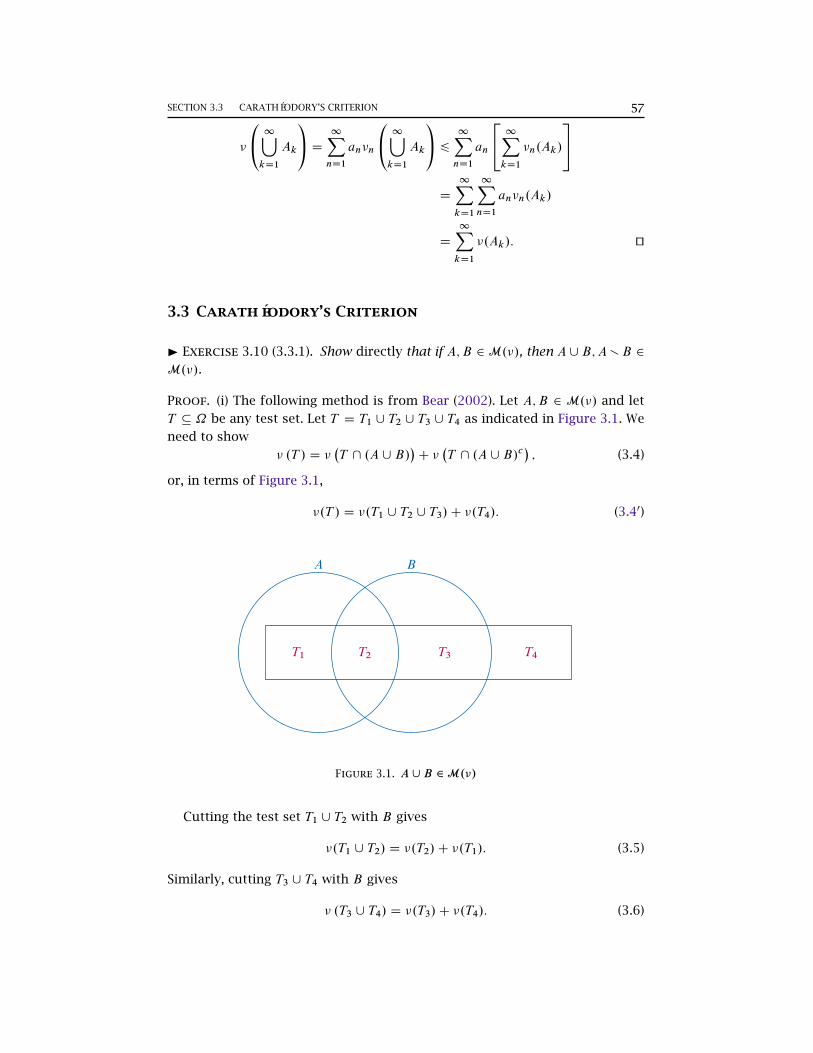
SECTION 3.3 CARATHÉODORY’S CRITERION 57
�
0@ 1[kD1
Ak
1A D 1XnD1
an�n
0@ 1[kD1
Ak
1A 6 1XnD1
an
24 1XkD1
�n.Ak/
35D
1XkD1
1XnD1
an�n.Ak/
D
1XkD1
�.Ak/: ut
3.3 Carathéodory’s Criterion
I Exercise 3.10 (3.3.1). Show directly that if A;B 2M.�/, then A[B;AXB 2
M.�/.
Proof. (i) The following method is from Bear (2002). Let A;B 2 M.�/ and let
T � ˝ be any test set. Let T D T1 [ T2 [ T3 [ T4 as indicated in Figure 3.1. We
need to show
� .T / D ��T \ .A [ B/
�C �
�T \ .A [ B/c
�; (3.4)
or, in terms of Figure 3.1,
�.T / D �.T1 [ T2 [ T3/C �.T4/: (3.40)
T1 T2 T3 T4
A B
Figure 3.1. A[B 2M.�/
Cutting the test set T1 [ T2 with B gives
�.T1 [ T2/ D �.T2/C �.T1/: (3.5)
Similarly, cutting T3 [ T4 with B gives
� .T3 [ T4/ D �.T3/C �.T4/: (3.6)
58 CHAPTER 3 EXTENSIONS OF MEASURES
Cutting T with A gives
�.T / D �.T1 [ T2/C � .T3 [ T4/ : (3.7)
Combining (3.5), (3.6), and (3.7) we can write
�.T / D �.T1/C �.T2/C �.T3/C �.T4/: (3.8)
Now cut T1 [ T2 [ T3 with A and then use (3.5):
�.T1 [ T2 [ T3/ D �.T1 [ T2/C �.T3/ D �.T1/C �.T2/C �.T3/: (3.9)
From (3.9) and (3.8) we have the desired equality (3.40).
(ii) It is clear that A 2 M.�/ iff Ac 2 M.�/. Thus, A;B 2 M.�/ implies that
B [ Ac 2M.�/ by the previous result. Since A X B D .B [ Ac/c 2M.�/, we get
A X B 2M.�/. ut
I Exercise 3.11 (3.3.2). Suppose that ˝ may be written asS1nD1An, where
fAng1nD1 is a nondecreasing sequence of subsets of ˝. If A � ˝ is such that
A \ Ak 2M.�/ for all k exceeding some constant kA, then A 2M.�/.
Proof. By the Outer Measure Theorem, M.�/ is a � -field on ˝. Therefore,
1[kDkAC1
.A \ Ak/ D A \
0@ 1[kDkAC1
Ak
1A 2M.�/:
But since fAkg1kD1 is a nondecreasing sequence, we have
1[kDkAC1
Ak D
1[kD1
Ak D ˝;
which means that
A \
0@ 1[kDkAC1
Ak
1A D A \˝ D A 2M.�/: ut
I Exercise 3.12 (3.3.3). Let � denote an outer measure such that �.˝/ < C1,
and further suppose that if A � ˝ with �.A/ < C1, then there exists B 2M.�/
such that A � B and �.A/ D �.B/. Then E 2M.�/ iff �.˝/ D �.E/C �.Ec/.
Proof. If E 2M.�/, then �.T / D �.T \E/C� .T \Ec/; in particular, this holds
for T D ˝, so �.˝/ D �.E/C �.Ec/.
For the other direction, suppose �.˝/ D �.E/C �.Ec/. Since �.˝/ < C1, we
get �.E/; �.Ec/ < C1 by the monotonicity of �. Then there exist B 0; B 00 2M.�/
such that Ec � B 0, �.Ec/ D �.B 0/, and E � B 00, �.E/ D �.B 00/. Let B D .B 0/c 2
M.�/. Then B � E and
�.B/ D �..B 0/c/ D �.˝/ � �.B 0/ D��.E/C �.Ec/
�� �.Ec/ D �.E/:

SECTION 3.3 CARATHÉODORY’S CRITERION 59
Hence, there exist B;B 00 2 M.�/ such that B � E � B 00, and �.B/ D �.E/ D
�.B 00/.
Notice that E is the union of B and a subset of B 00 X B . If we can show that
every subset of B 00 X B is in M.�/, then E 2 M.�/ (since M.�/ is a � -field). For
every C � B 00 X B , we have
�.C / 6 �.B 00 X B/ D �.B 00/ � �.B/ D 0:
Therefore, �.C / D 0, i.e., C 2M.�/, and so E 2M.�/. ut
I Exercise 3.13 (3.3.4). Suppose that � is an arbitrary outer measure, and let
A;B � ˝ with A 2M.�/. Show that �.A [ B/C � .A \ B/ D �.A/C �.B/.
Proof. A 2M.�/ implies that
�.A [ B/ D ��.A [ B/ \ A
�C �
�.A [ B/ \ Ac
�D �.A/C �
�B \ Ac
�; (3.10)
and
�.B/ D �.B \ A/C ��B \ Ac
�: (3.11)
Combining (3.10) with (3.11) we get �.A [ B/C � .A \ B/ D �.A/C �.B/. ut
I Exercise 3.14 (3.3.5). Let � denote an outer measure, and let fAng1nD1 denote
a nondecreasing sequence of M.�/-sets. Show that �.lim.A \ An// D lim �.A \
An/ for any A � ˝. State and prove an analogous result for nonincerasing
sequences of M.�/-sets.
Proof. Let fAng1nD1 be a nondecreasing sequence of M.�/-sets. Then fA \ Ang
forms a nondecreasing sequence, so lim.A \ An/ DS.A \ An/ D A \ .
SAn/.
Let B1 D A1 and Bn D An XAn�1 for n > 2. Then fBng �M.�/ is disjoint andSAn D
SBn. Thus
��lim.A \ An/
�D �
�A \
�[Bn
��D
1XnD1
�.A \ Bn/
D limn
nXiD1
�.A \ Bn/
D limn�
0B@A \0@ n[iD1
Bi
1A1CA
D limn�.A \ An/:
If fAng is a nonincreasing sequence of M.�/ sets, then fAcng is a nondecreas-
ing sequence of M.�/ sets. Thus �.lim.A X An// D lim �.A X An/. ut
I Exercise 3.15 (3.3.6). Let � denote an outer measure such that the following
holds: if A � ˝ with �.A/ < C1, then there is B 2 M.�/ with A � B and
60 CHAPTER 3 EXTENSIONS OF MEASURES
�.A/ D �.B/. Then, for any nondecreasing sequence fAng1nD1 of subsets of ˝, we
have �.limAn/ D lim �.An/.
Proof. If there exists Ak such that �.Ak/ D C1, then �.limAn/ D �.SAn/ >
�.Ak/ D C1, and so �.limAn/ D C1; on the other hand, � .A1/ 6 � .A2/ 6 � � �and �.Ak/ D C1 imply that lim �.An/ D C1.
Now let �.An/ < C1 for all n 2 N. Then there exists Bn 2 M.�/ such that
An � Bn and �.An/ D �.Bn/ for each n 2 N. We first show that we can choose
fBng so that it is nonincreasing.
Consider Bn and BnC1. If Bn � BnC1, then �.Bn/ D �.BnC1/ since �.Bn/ D
�.An/ 6 �.AnC1/ D �.BnC1/ always holds. But then �.An/ D �.AnC1/ and so we
can just let BnC1 D Bn after we having chosen Bn.
Thus, �.limBn/ D lim �.Bn/ exists. Since fAng1nD1 is nondecreasing, we
have �.SniD1Ai / D �.An/ D �.Bn/ for all n 2 N. Take the limit and we get
��S1
iD1Ai�D �.limBn/ D lim �.Bn/ D lim �.An/. ut
I Exercise 3.16 (3.3.7). In each of the following parts, (i) describe the outer
measure �� on 2˝ induced by the given �, (ii) describe the collection M.��/ and
determine if M.��/ is a � -field, and (iii) check to see whether �� D � on the
given collection A.
a. ˝ D f1; 2; 3g, A D˚¿; f1g ; f2; 3g ; ˝
, and � is a measure on A such that
�.˝/ D 1 and ��f1g�D 0.
Solution. (a) Since � is a measure on A, by (finite) additivity, �.¿/ D 0 and
��f2; 3g
�D �.˝/ � �
�f1g�D 1. Then, �� .¿/ D 0, ��
�f1g�D 0, ��
�f2; 3g
�D 1,
��.˝/ D 1, ���f2g�D �
�f2; 3g
�D 1, �� .3/ D �
�f2; 3g
�D 1, ��
�f1; 2g
�D
���f1; 3g
�D �.˝/ D 1. ut
3.4 Existence of Extensions
I Exercise 3.17 (3.4.1). Let k 2 N and refer to the measure �k W Bk ! xR that
assigns the valueQkiD1 .bi � ai / to every .a;b� 2 Ak , as given in this section’s
example. For this measure �k , we have the following;
a. �k�.a;b�
�D �k
�.a;b/
�D �k
�Œa;b/
�D �k
�Œa;b�
�DQkiD1 .bi � ai /.
b. �k applies to any k-dimensional rectangle that contains a k-dimensional open
set and is unbounded in at least one dimension gives C1.
c. �k applied to any bounded Bk-set yields a finite number.
d. It might be thought that if A � B with B 2 Bk with �k.B/ D 0, then �k.A/
must exists and equal 0. Show that if there exists an uncountable set C 2 Bk
with �k.C / D 0, then �k.A/ need not even exist, let along equal zero, and thus
�k violates our intuition in this regard.
SECTION 3.4 EXISTENCE OF EXTENSIONS 61
Proof. (a) Observe first that fxg D limn
�x � 1=n;x
�for any x 2 Rk . Therefore,
�k�fxg
�D �k
�limn
�x � 1=n;x
��D lim
n�k�x � 1=n;x
�D lim
n1=nk D 0:
Now by (M5),
�k .a;b/ D �k�.a;b� X fbg
�D �k .a;b� � �k
�fbg�D �k .a;b� :
(b) Write .a;b� D .a1; b1�� � � � .ak ; bk �, and assume that b1 � a1 D1. Since .a;b�
contains an open set, bi � ai > 0 for each i D 1; : : : ; k. Therefore, �.a;b� D1.
(c) Let A 2 Bk be bounded. Then there exists a bounded .a;b� containing A.
Hence �k.A/ 6 �k.a;b� <1.
(d) By the Continuum Hypothesis, if C is countable then jC j > c. Henceˇ̌̌2Cˇ̌̌>
2c > c. However, jBkj D c. ut
I Exercise 3.18 (3.4.2). This problem reviews the Extension Theorem.
a. Where or how is the fact that �.¿/ D 0 used?
b. What happens if A D 2˝?
Solution. (a) ¿ 2M���
and (b) The Extension Theorem holds if and only if �
is a measure on A. ut
I Exercise 3.19 (3.4.3). Consider the Extension Theorem framework. If we have
�.A/ < C1 for each A 2 A, it might not be the case that the measure extension
���.A/
assigns finite measure to every set in �.A/. However, if � is � -finite on A,
then the measure extension ���.A/
is � -finite on �.A/, and the measure extension
��M.��/
is � -finite on M.��/.
Proof. Let ˝ D R and A consist of ¿ and all bounded rsc intervals .a; b�. Let
�.a; b� D b � a for all .a; b� 2 A. Then �.A/ < C1 for each A 2 A. However,
R 2 � .A/, and ���.A/
.R/ D C1. The other two claims are obvious. ut
I Exercise 3.20 (3.4.4). There is a measure � W B ! xR with �.R/ D 1 and
�.a; b� D
Z b
a
.2�/�1=2 e�z2=2 dz;
where the integral is the familiar Riemann integral from calculus.
Proof. According to the approach of Georgakis (1994), let y D zs, dy D z ds,
then
62 CHAPTER 3 EXTENSIONS OF MEASURES Z b
a
e�z2=2 dz
!2D
Z b
a
Z b
a
e�.z2Cy2/=2 dy
!dz
D
Z b
a
Z b
a
e�z2.1Cs2/=2z ds
!dz
D
Z b
a
Z b
a
e�z2.1Cs2/=2z dz
!ds
D
Z b
a
24 1
��1C s2
�e�z2.1Cs2/=2 ˇ̌̌̌ˇb
a
35 ds
D
Z b
a
1
1C s2e�a
2.1Cs2/=2 ds �
Z b
a
1
1C s2e�b
2.1Cs2/=2 ds: ut
I Exercise 3.21 (3.4.5). Consider the Extension Theorem framework again.
a. If A � B � ˝ with B 2 M.��/ and ��M.��/
.B/ D 0, then A 2 M.��/ and
��M.��/
.A/ D 0.
b. If in (a) we replace every occurrence of M.��/ [including instances where it
appears as a subscript] with �.A/, then the claim is not necessarily true.
Proof. (a) Assume the hypotheses. To see A 2M.��/, note that for any T � ˝
with �� .T / < C1, we have ��.T\A/ 6 ��.T\B/ 6 ��.B/ D 0 by monotonicity
of ��. Therefore, ��.T / > ��.T \ A/C ��.T \ Ac/ D ��.T \ Ac/ always holds.
(b) The same reason as in Exercise 3.17(d). ut
I Exercise 3.22 (3.4.6). Let F denote a field on ˝, and let � W F ! xR denote a
measure. Let �� W 2˝ ! xR be given by
��.A/ D inf
8<:1XnD1
�.An/ W fAng is a F -covering of A
9=; ; A � ˝:
Then �� is an outer measure, and the restriction of �� to the � -field M.��/ is a
measure. With these facts, we have that �� D � on F and F � M.��/. Finally,
there exists a measure extension of � to �.F /.
Proof. Notice that �.¿/ D 0 and �.A/ > 0 for all A 2 F since � is a measure
on F . So �� is an outer measure by Example 1 in Section 3.2. The other parts
are standard. ut
I Exercise 3.23 (3.4.7). Let F denote a field on ˝. Suppose that � W F ! xR is
such that (i) �.A/ > 0 for all A 2 F , (ii) � is finitely additive, and (iii) if fAng1nD1 is
a nonincreasing sequence of F -sets with limAn D ¿, the lim �.An/ D 0. Define
�� W 2˝ ! xR for all A � ˝ by writing
��.A/ D inf
8<:1XnD1
�.An/ W fAng1nD1 is an F -covering of A
9=; :
SECTION 3.5 UNIQUENESS OF MEASURES AND EXTENSIONS 63
a. �� is an outer measure.
b. M.��/ is a � -field on ˝.
c. The restriction of �� to M.��/ is a measure on M.��/.
d. F �M.��/.
e. There exists a measure extension of � to � .F /.
Proof. (a) It suffices to show that � .¿/ D 0 by Example 1 of Section 3.2. Take
a sequence f¿;¿; : : :g. Then 0 D lim � .¿/ D �.¿/.
(b) —(e) are from the Outer Measure Theorem. ut
3.5 Uniqueness of Measures and Extensions
I Exercise 3.24 (3.5.1). If �1 and �2 are finite measures with domain �.P /
(where P denotes a �-system on ˝), if ˝ can be expressed as an amc union of
P -sets, and if �1 D �2 on P , then �1 D �2 on �.P /.
Proof. Assume the hypotheses. Then �1 is � -finite with respect to P and �1 D
�2 on P . By the Uniqueness Theorem, �1 D �2 on �.P /. ut
I Exercise 3.25 (3.5.2). Let �1 and �2 denote finite measures with domain
�.P /, where P is a �-system on ˝, and further suppose that �1 D �2 on P .
Then �1 D �2.
Proof. I am not sure about this exercise. If ˝ 2 P , then by letting
L D fA 2 �.P / W �1.A/ D �2.A/g ;
we can easily to show that L is a �-system with P � L. Then the result is
trivial. ut
I Exercise 3.26 (3.5.3). Let ˝ D f!1; !2; !3; !4g, let A consist of ¿, f!1; !2g,
f!1; !3g, f!2; !4g, f!3; !4g, and ˝, and let � W A ! R be defined as follows:
�.˝/ D 6, �.¿/ D 0, and �.f!1; !2g/ D �.f!1; !3g/ D �.f!2; !4g/ D �.f!3; !4g/ D
3.
a. A is neither a �-system nor a semiring, and �.A/ D 2˝ .
b. � is a measure.
c. Define two new distinct measures � and � on the � -field 2˝ by the following:
�.f!1g/ D �.f!4g/ D 1, �.f!2g/ D �.f!3g/ D 2, �.f!2g/ D �.f!3g/ D 1, and
�.f!1g/ D �.f!4g/ D 2. Then � and � are distinct measure extensions of �
from A to �.A/ D 2˝ .
64 CHAPTER 3 EXTENSIONS OF MEASURES
d. Let �� W 2˝ ! R denote the outer measure induced by �. Then �� D � on A
and �� is a measure.
e. ��, �, and � are distinct measures.
Proof. (a) A is not a �-system because f!1; !2g \ f!1; !3g D f!1g … A, and so
A is not a semiring. �.A/ D 2˝ since every singleton can be expressed as a
intersection of A-sets.
(b) Easy to check.
(c) For example, �.f!1; !g/ D �.f!1g/C �.f!2g/ D 1C 2 D �.f!1; !2g/.
(d) For example, ��.f!g/ D inff�.f!1; !2g/; �.f!1; !3g/g D 3.
(e) Trivial to see that they are distinct. ut
I Exercise 3.27 (3.5.5). We assume the setup of Exercise 3.22. The aim of this
exercise is to show that if � is a measure with domain �.F / such that � D � on
the field F , then � coincides with the measure extension of � to �.F / guaranteed
by Exercise 3.22.
a. If B 2 �.F /, then �.B/ 6 ��.B/.
b. If F 2 �.F / and ��.F / < C1, then �.F / D ��.F /.
c. If � is � -finite on F , then �.E/ D ��.E/ for all E 2 �.F /. This gives the
uniqueness of the measure extension whose existence is guaranteed by Exer-
cise 3.22.
Proof. (a) Let F� denote the family of all countable unions of F -sets. If A 2
F� , i.e., A DSAn with An 2 F for all n, then, by letting B1 D A1 and Bn D
An X .Si6nAi / for n > 2, we can rewrite A as a disjoint union of F -sets fBng.
Thus,
�.A/ D ��[
Bn
�D
X�.Bn/ D
X�.Bn/ D
X��.Bn/ D �
��[
Bn
�D ��.A/:
Now take an arbitrary B 2 �.F /, and we show that
��.B/ D infnX
�.An/ W fAng is an F -covering of Bo
D inf˚��.A/ W B � A 2 F�
defined as ˇ:
Firstly, B � A implies that ��.B/ 6 ��.A/ and so ��.B/ 6 ˇ. Secondly, for all
A 2 F� , there exists fAng � F� such that A DSAn, and so we get ��.A/ D
��.SAn/ 6
P��.An/ D
P�.An/; thus, ˇ 6 ��.B/. Therefore,
��.B/ D inf˚��.A/ W B � A 2 F�
D inf f�.A/ W B � A 2 F�g > �.B/:
SECTION 3.5 UNIQUENESS OF MEASURES AND EXTENSIONS 65
(b) It suffices to show that �.F / > ��.F / by part (a). Since ��.F / D inff��.A/ W F �
A 2 F�g, for a given " > 0, there exists C 2 F� with F � C , such that
��.F /C " > ��.C /:
Hence,
��.F / 6 ��.C / D �.C / D �.F /C �.C X F / 6 �.F /C ��.C X F /D �.F /C ��.C / � ��.F /
< �.F /C ":
Since " > 0 is arbitrary, we get ��.F / 6 �.F / whenever F 2 �.F / and ��.F / <
C1.
(c) If � is � -finite on F , then there exists fAng � F such that ˝ DSAn and
�.An/ < C1 for all n. Without loss of generality, we can assume that fAng is
disjoint F -sets. Then by (b), for every E 2 �.F / we get
�.E/ D ��[
.E \ An/�D
X�.E \ An/ D
X��.E \ An/ D �
�.E/: ut
I Exercise 3.28 (3.5.6). A lattice on ˝ is a collection L � 2˝ such that (i)
˝ 2 L, (ii) ¿ 2 L, (iii) L is closed under (finite) unions, and (iv) L is a �-system.
We also define the following two collections: D D fB XA W A;B 2 L; A � Bg, and
U will denote the collection of all finite disjoint unions of D-sets.
a. D is a �-system.
b. U is a �-system.
c. U is closed under complementation.
d. U coincides with the minimal field containing the lattice L.
e. Let A denote a � -field on ˝ that contains L. Suppose that � and � are mea-
sures with domain A such that � D � on L. Furthermore, suppose that
˝ DSAn, where An 2 L and �.An/ < C1 for each n 2 N. Then � D �
on �.L/.
Proof. (a) Write Di D Bi X Ai with Ai ; Bi 2 L and Ai � Bi , for i D 1; 2. Then
D1 \D2 D .B1 X A1/ \ .B2 X A2/
D .B1 \ Ac1/ \ .B2 \ A
c2/
D .B1 \ B2/ X .A1 [ A2/
D .B1 \ B2/ X�.B1 \ B2/ \ .A1 [ A2/
�2 D :
66 CHAPTER 3 EXTENSIONS OF MEASURES
(b) Let U1 D D1 [ � � � [Dm and U2 D E1 [ � � � [ En, where D1; : : : ;Dm 2 D are
disjoint, and E1; : : : ; En 2 D disjoint. Then
U1 \ U2 D
m[iD1
n[jD1
.Di \Ej /:
Since Di \ Ej 2 D (D is a �-system), U1 \ U2 is a finite disjoint unions of
D-sets, and so is in U.
(c) Pick an arbitrary U 2 U. Then there exists disjoint D1; : : : ;Dn 2 D such
that U DSniD1Di . If n D 1, then U D D1 D B1 X A1, where A1; B1 2 L and
A1 � B1. Thus, U c D .A X¿/ [ .˝ X B/ 2 U. Let us assume that U c 2 U when
U D D1 [ � � � [Dn and consider nC 1. Then0@nC1[iD1
Di
1Ac D0@ n[iD1
Di
1Ac \DcnC1 2 U;
since .SniD1Di /
c 2 U by the induction hypothesis, DcnC1 2 U as in the case of
nC 1, and U is a �-system.
(d) Notice that ˝ D ˝ X ¿ 2 U, so U is a field by (b) and (c). If A 2 L, then
A D A X¿ 2 U, so L � U. Thus, f .L/ � U. It is easy to see that U � f .L/.
(e) Let ˝ DS1nD1An with An 2 L and �.An/ < C1 for each An. Let U 2 U;
then U D D1 [ � � � [Dm for some disjoint D1; : : : ;Dm 2 D . Hence,
�.U / D �
0@ 1[nD1
.An \ U/
1A D 1XnD1
�.An \ U/
D
1XnD1
mXiD1
�.An \Di /
ut
3.6 The Completion Theorem
I Exercise 3.29 (3.6.1). Let k > 2, and let �k W Bk ! xR denote the unique mea-
sure with domain Bk that assigns the valueQkiD1.bi �ai / to each k-dimensional
rsc rectangle .a;b�. Let A D fx 2 Rk W x2 D � � � D xk D 0g. Then A 2 Bk , A is
uncountable, and �k.A/ D 0, henceˇ̌̌Bkˇ̌̌D 2c.
Proof. A 2 Bk since A D limnŒ.�n; n�� .�1=n; 1=n�k�1�; A is uncountable since
R is uncountable; �k.A/ D 0 since �k.A/ D .C1/ � 0 � � � � � 0 D 0.
Since Bk is complete (the completion of Bk), and A 2 Bk � Bk , we know
that every subset of A is in Bk . There are 2c subsets of A, soˇ̌̌Bk
ˇ̌̌> 2c; on
SECTION 3.7 THE RELATIONSHIP BETWEEN �.A/ AND M.��/ 67
the other hand, there are 2c subsets on R, i.e.,ˇ̌̌Bk
ˇ̌̌6 2c. It follows from the
Cantor-Bernstein theorem thatˇ̌̌Bk
ˇ̌̌D 2c. ut
I Exercise 3.30 (3.6.2). Let .˝;F ; �/ denote a measure space. If A;B 2 F with
A � E � B and �.B X A/ D 0, then E 2 xF and x�.E/ D �.A/ D �.B/.
Proof. We first show E 2 xF . Since A;B 2 F , and F is a � -field, we get B XA 2
F . Now we can write E as
E D A [�.B X A/ X .B XE/
�:
Since A 2 F , .B X A/ X .B X E/ � B X A 2 F , and �.B X A/ D 0, we have
.B X A/ X .B XE/ 2 N0.�/; thus E 2 xF .
To show x�.E/ D �.A/ D �.B/, we only need to show that �.A/ D �.B/ since
x�.E/ D �.A/ by definition. If �.A/ < C1 or �.B/ < C1, then 0 D �.B X A/ D
�.B/ � �.A/ implies that �.B/ D �.A/. If �.A/ D C1, then by the monotonicity
of a measure, �.B/ > �.A/ D C1, and so �.B/ D C1 D �.A/ ut
I Exercise 3.31 (3.6.3). Let .˝;F ; �/ denote a measure space. Furthermore,
let F1 denote a sub-� -field of F . Then there exists a minimal � -field F2 such
that F1 � F2 � F and N .�/ � F2. Also, A 2 F2 iff there exists B 2 F1 with
A�B 2 N .�/.
Proof. Let F2 D �.F1;N .�//. It is clear that F1;N .�/ � F2. Since F1;N .�/ � F ,
we have that
F2 D �.F1;N .�// � �.F / D F :
We next show that .˝;F2; �/ is complete (where � is restricted on F2). ut
3.7 The Relationship between �.A/ and M.��/
I Exercise 3.32 (3.7.1). Let ˝ be uncountable, let A denote the � -filed fA �
˝ W A is amc or Ac is amsg, and define � W A ! xR by stipulating that �.A/ de-
notes the number of points in A if A is finite and �.A/ D C1 if A is infinite.
a. .˝;A; �/ is a non-� -finite measure space.
b. .˝;A; �/ is complete.
c. Letting �� denote the outer measure induced by �, the (� -field) M.��/ coin-
cides with 2˝ .
Proof. (a) For every sequence fAng � A with �.An/ < C1, i.e., An is finite for
all n, their unionSnAn is amc. Hence, .˝;A; �/ is non-� -finite.
(b) Let A � B � ˝ with B 2 A and �.B/ D 0. Then B must be empty and so
A D ¿ D B 2 A.
68 CHAPTER 3 EXTENSIONS OF MEASURES
(c) Take an arbitrary T � ˝ with ��.T / < C1; that is, T is finite. Then for
every subset A � ˝, we have that T \ A and T \ Ac are both finite and jT j D
jT \ AjCjT \ Ac j. Hence, ��.T / D ��.T \A/C��.T \Ac/, i.e., A 2M.��/. Thus,
M.��/ D 2˝ .
Note that here xA D A ¤M.��/ D 2˝ , so the � -finiteness is essential. ut
3.8 Approximations
I Exercise 3.33 (3.8.1). The assumption �.B/ < C1 is not superfluous in Claim
4, and the assumption �.A/ < C1 is not superfluous in Claim 6.
Proof. Let A be the semiring consisting of ¿ and all bounded rsc .a; b�. Let
us consider .R;B; �/. For Claim 4, take B D R. It is evident that for any finite
disjoint A-sets .a1; b1�; : : : ; .an; bn�, we have �.R�SniD1.ai ; bi �/ D C1. For Claim
6, let A D R. then for any bounded set E 2 B, there exists .a; b� 2 A containing
E, so �.E/ 6 �.a; b� D b � a < C1 D �.R/. ut
I Exercise 3.34 (3.8.2). Let � W Bk ! xR be nonnegative and finitely additive
with �.Rk/ < C1. Suppose that �.A/ D supf�.K/ W K � A;K compactg for each
A 2 Bk . Then � is a finite measure.
Proof. It suffices to show that � is countably additive. ut
3.9 A Further Description of M.��/
I Exercise 3.35 (3.9.1). Countable superadditivity: If A1; A2; : : : � ˝ are dis-
joint, then ��.S1nD1An/ >
P1nD1 ��.An/.
Proof. Fix an arbitrary " > 0. For every An, find Cn 2 �.A/ with Cn � An such
that
���.A/.Cn/C "=2n > ��.An/:
SinceS1nD1 Cn �
S1nD1An, we have
1XnD1
��.An/ <
1XnD1
���.A/.Cn/C " D ���.A/
0@ 1[nD1
Cn
1AC " 6 ��0@ 1[nD1
An
1AC ";where the first equality holds since fCng is disjoint �.A/-sets. Since " > 0 is
arbitrary, we get the countable superadditivity. ut
I Exercise 3.36 (3.9.2). For any A � ˝, ��.A/ D inff��M.��/
.B/ W A � B 2
M.��/g D ���.A/.
Proof. Define
SECTION 3.9 A FURTHER DESCRIPTION OF M.��/ 69
C Dn���.A/.B/ W A � B 2 �.A/
oand D D
n��M.��/.B/ W A � B 2M.��/
o:
It is clear that C � D , so inf C > inf D . Next, pick d 2 D . Then d must be of
the form ��M.��/
.B/, where A � B 2M.��/. Write B D C [D, where C 2 �.A/,
D � N and N is a ���.A/
-null set. Thus, there exists C [ N 2 �.A/ such that
A � B � C [N and
���.A/.C [N/ 6 ���.A/.C /C �
��.A/.N / D �
�M.��/.C / 6 �
�M.��/.B/:
Denote ���.A/
.C [N/ D c. Hence, for every d 2 D , there exists c 2 C with c 6 d .
It follows that inf C 6 inf D . ut
I Exercise 3.37 (3.9.3). For any A � ˝, ��.A/ D supf��M.��/
.B/ W B � A;B 2
M.��/g.
Proof. Define
C Dn���.A/.B/ W B � A;B 2 �.A/
o; D D
n��M.��/.B/ W B � A;B 2M.��/
o:
First, C � D implies that sup C 6 sup D . Next, pick d 2 D . Then d must be
of the form ��M.��/
.B/, where B � A and B 2 M.��/. Write B D C [ D with
C 2 �.A/, D � N , and N is a ���.A/
-null set. Thus, there exists C 2 �.A/ such
that C � B � A, and
���.A/.C / D ��M.��/.C [D/ D �
�M.��/.B/:
Denote c D ���.A/
.C /. So for every d 2 D there exists c 2 C such that c D d .
Therefore, sup C > sup D . ut
I Exercise 3.38 (3.9.4). For any A � ˝, there is E 2 �.A/ such that E � A and
���.A/
.E/ D ��.A/.
Proof. For every n 2 N, there exists En 2 �.A/ with En � A such that
���.A/.En/ > ��.A/ � 1=n:
Let E DS1nD1En. Then E 2 �.A/, E � A, and for all n we have
���.A/.E/ > ���.A/.An/ > ��.A/ � 1=nI
hence, ���.A/
.E/ > ��.A/. Since ���.A/
.E/ 6 ��.A/ holds, we get the result. ut
I Exercise 3.39 (3.9.5). The infimum that defines ��.A/ and the supremum
that defines ��.A/ are achieved for each A � ˝. That is, there exist C;B 2 �.A/
with C � A � B and ���.A/
.C / D ��.A/ and ���.A/
.B/ D ��.A/.
Proof. We have proved the inner measure in the previous exercise, so we
focus on the outer measure. For every n 2 N, there exists Bn 2 �.A/ with
70 CHAPTER 3 EXTENSIONS OF MEASURES
A � Bn and ��.A/C 1=n > ���.A/
.Bn/. Let B DT1nD1 Bn. Then B 2 �.A/, A � B ,
and for all n,
���.A/.B/ 6 ���.A/.Bn/ 6 �
�.A/C 1=nI
that is, ���.A/
.B/ 6 ��.A/. Since the other direction is clear, we get the result.
ut
I Exercise 3.40 (3.9.6). Let A � ˝ and let fAng denote a disjoint sequence of
M.��/-sets. Then we have ��.S1nD1.A \ An// D
P1nD1 ��.An \ A/.
Proof. There exists E 2 M.��/ with E �S1nD1.A \ An/ D A \ .
S1nD1An/ and
��M.��/
.E/ D ��.S1nD1.A \ An// by Exercise 3.38 (since �.A/ DM.��/). Thus,
��
0@ 1[nD1
.A \ An/
1A D ��M.��/.E/ D
1XnD1
��M.��/.E \ An/ 61XnD1
��.A \ An/:
Then the desired result follows from Exercise 3.35. ut
I Exercise 3.41 (3.9.7). If A;B � ˝ are disjoint, then ��.A [ B/ 6 ��.A/ C
��.B/ 6 ��.A [ B/.
Proof. Let F 2 �.A/ with B � F with ��.B/ D ���.A/
.F /. Let E 2 �.A/ with
E � A[B such that ��.A[B/ D ���.A/.E/. SinceEXF � EXB � .A[B/XB D A,
it follows that
��.A [ B/ D ���.A/.E/ 6 �
��.A/.E X F /C �
��.A/.F / 6 ��.A/C �
�.B/:
Dually, let H 2 �.A/ with H � A and ���.A/
.H/ D ��.A/. Let G 2 �.A/ with
A [ B � G and ���.A/
.G/ D ��.A [ B/. Since B � G XH , it follows that
��.A [ B/ D ���.A/.G/ D ���.A/.H/C �
��.A/.G XH/ > ��.A/C �
�.B/: ut
I Exercise 3.42 (3.9.8). If A 2 M.��/ and B � ˝, then ��M.��/
.A/ D ��.B \
A/C ��.Bc \ A/:
Proof. Applying Exercise 3.41 to B \ A and Bc \ A, we obtain
��.A/ 6 ��.B \ A/C ��.Bc \ A/ 6 ��.A/:
Since A 2 M.��/, we have ��.A/ D ��.A/ D ��M.��/
.A/, and thus we get the
result. ut
4LEBESGUE MEASURE
4.1 Lebesgue Measure: Existence and Uniqueness
I Exercise 4.1 (4.1.1). Let x 2 R and k > 2. Then �.fxg/ D �k.fxg � Rk�1/ D 0.
Next, for any j 2 f1; : : : ; k � 1g and x 2 Rj we have �k.fxg � Rk�j / D 0.
Proof. Since the sequence ffxg � .�n; n�k�1g is increasing and converges to
fxg � Rn�1, we have
�k.fxg � Rk�1/ D �k.limnfxg � .�n; n�k�1/ D 0 D �.fxg/:
The other claim can be proved in the same way. ut
I Exercise 4.2 (1.4.2). Enumerate the rationals in .0; 1� by fq1; q2; : : :g. Given
arbitrarily small " > 0, remove the interval An D .qn�"=2nC1; qnC"=2nC1/\.0; 1�.
Let A DS1nD1An. Then x�.A/ 6 ", despite the fact that A is an open dense subset
of .0; 1�. Also, we have x�..0; 1� X A/ > 1 � ", even though .0; 1� X A is a nowhere
dense subset of .0; 1�.
Proof. For every An we have 0 < x�.An/ 6 x�.qn � "=2nC1; qn C "=2nC1/ D "=2n;
hence,
x�.A/ D x�
0@ 1[nD1
An
1A 6 1XnD1
� .An/ 61XnD1
"
2nD ";
and so x�..0; 1� X A/ D 1 � x�.A/ > 1 � ". ut
I Exercise 4.3 (4.1.3). There cannot exist a closed subset of .0; 1� whose interior
is empty, yet has x�-measure of one.
Proof. ut
I Exercise 4.4 (4.14). �k is nonatomic: any A 2 Bk with �k.A/ > 0 has a proper
subset B 2 Bk with 0 < �k.B/ < �k.A/. This forces x�k to be nonatomic as well.
71
72 CHAPTER 4 LEBESGUE MEASURE
Proof. Take any A 2 Lk with x�k.A/ > 0. Since Lk D Bk , the completion of Bk ,
there exists C;M 2 Bk , whereM is a subset of �k-null set, such that A D C[B .
Therefore, �k.B/ D x�k.A/ > 0. Since �k is nonatomic, there exists B 2 Bk with
0 < �k.B/ < �k .C / D x�k.A/, that is, x�k is nonatomic. ut
I Exercise 4.5 (4.1.5). Let k > 2. There exists an uncountable set U 2 Bk with
�k.U / D 0.
Proof. Let U D fxg�R, where x 2 R. Then U is uncountable, and �.U / D 0. ut
I Exercise 4.6 (4.1.6). jLkj D 2c and jBkj D c for each k 2 N.
Proof. Since jRkj D c and Lk � 2Rk , we first have jLkj 6 2c; on the other hand,
there exists an uncountable set U � Rk such that �k.U / D 0 (if k D 1, consider
the Cantor set; if k > 2, consider the set U in the preceding exercise), so jU j D c
by the Continuum Hypothesis. Since Lk is complete, we have jLkj > j2U j D 2c.
It follows from the Cantor-Bernstein Theorem that jLkj D 2c. ut
I Exercise 4.7 (4.1.7). Assume that L D 2R; in particular every one of the 2c
subsets of Œ0; 1� is a Lebesgue set. Let B D fx�.A/ W A � Œ0; 1�; x�.A/ … Ag. Consider-
ation of the set B (which is in L be assumption) leads to contradiction.
Proof. B � Œ0; 1� so x�.B/ exists. We now have a contradiction: x�.B/ 2 B iffx�.B/ … B . ut
I Exercise 4.8 (4.1.8). Let k > 2. Every line is in Bk , has �k-measure zero, and
hence has x�k-measure.
Proof. Let ` be the line. Take two points a and b in `, and denote Œa;b� as the
segment on `. Then Œa;b� is closed in Rk and so is in Bk . Enumerate the points
with rational coordinates on Œa;b�; then it is easy to see that x�k.Œa;b�/ D 0.
Write ` as an increasing limit of line segments containing Œa;b�. Then we get
the result. ut
I Exercise 4.9 (4.1.9). Let B.0;1� D �.f.a; b� W .a; b� � .0; 1�g/.
a. B.0;1� D fB � .0; 1� W B 2 Bg and B.0;1� D fB � .0; 1� W B 2 Lg.
b. Construct Lebesgue measure on both B.0;1� and B.0;1�. Call these measures
�.0;1� and x�.0;1�, and denote B.0;1� by L.0;1�.
c. �.0;1� as constructed is the measure restriction of � from B to B.0;1� and x�.0;1�as constructed is the measure restriction of x� from L to L.0;1�.
Proof. See, for example, Resnick (1999, Theorem 1.8.1). ut
SECTION 4.3 TRANSLATION INVARIANCE OF LEBESGUE MEASURE 73
4.2 Lebesgue Sets
No exercise.
4.3 Translation Invariance of Lebesgue Measure
I Exercise 4.10 (4.3.2). Let A 2 L be such that x�.A/ > 0, and let c 2 Œ0; 1/.
There exists an open interval U such that x�.A \ U/ > c�.U /.1
Proof. It follows from the Approximation Theorem for Lebesgue measure that
x�.A/ D inff�.G/ W G open, A � Gg:
Then for any " > 0, there exists an open set G containing A such that �.G/ <x�.A/ C "�.G/, i.e., .1 � "/�.G/ < x�.A/. Thus, for an arbitrary c 2 Œ0; 1/, there
exists an open set G containing A such that
c�.G/ 6 x�.A/:
Write G as an countable disjoint unions of open intervals: G DSGn. Then
x�.A/ D x�.A \G/ since A � G. We thus obtain
c�.G/ D c�
0@ 1[nD1
Gn
1A D 1XnD1
c�.Gn/ 6 x�.A/ D x�
0@ 1[nD1
.A \Gn/
1AD
1XnD1
x�.A \Gn/:
Hence, for some N 2 N, we must have c�.GN / 6 x�.A \ GN /. Let U D GN and
we are done. ut
I Exercise 4.11 (4.3.3). Let A 2 L contain an open interval. Then there exists
a > 0 such that .�a; a/ is contained in D.A/ D fx � y W x; y 2 Ag.
Proof. Let .b; c/ � A; then .b � c; c � b/ � D.A/. Let a D c � b and so .�a; a/ �
D.A/. ut
I Exercise 4.12 (4.3.4). Let A 2 L be such that x�.A/ > 0. Then there exists
a > 0 such that .�a; a/ is contained in D.A/ D fx � y W x; y 2 Ag.
Proof. It follows from Exercise 4.10 that there exists an open interval U � R
such thatx�.A \ U/ > 3�.U /=4:
We next show that a can be taken as �.U /=2.
1 Exercise 4.10—4.16 are from Halmos (1974).
74 CHAPTER 4 LEBESGUE MEASURE
(i) For an arbitrary x 2 .��.U /=2; �.U /=2/, the set U [ .U ˚ x/ is an open
interval containing .A \ U/ [ ..A \ U/˚ x/, and
�.U [ .U ˚ x// < �.U /C �.U /=2 D3
2�.U /:
(ii) .A\U/[..A\U/˚x/ is an interval. Suppose that .A\U/\..A\U/˚x/ D ¿;
then
x�..A \ U/ [ ..A \ U/˚ x// D x�.A \ U/C x�..A \ U/˚ x/
D 2x�.A \ U/
>3
2�.U /;
which contradicts the fact that x�..A \ U/ [ ..A \ U/˚ x// 6 �.U [ .U ˚ x// <3�.U /=2.
(iii) Thus, for every x 2 .��.U /=2; �.U /=2/, there exists y 2 .A \ U/ \ ..A \
U/ ˚ x/; that is, there exists y; z 2 A such that y D z C x. But then x D y � z
and so x 2 D.A/. Therefore, if we let a D �.U /=2, then .�a; a/ � D.A/. ut
I Exercise 4.13 (4.3.5). Let A be a dense subset of R. Then cA D fca W a 2 Ag is
dense for any c ¤ 0.
Proof. Take an arbitrary point x 2 R and an arbitrary open interval .x�"; xC"/.
Now consider .x � "=c; x C "=c/. Since A is dense, there exists a 2 A such that
a 2 .x � "=c; x C "=c/. Thus, ca 2 .x � "; x C "/ and ca 2 cA, i.e., cA is dense in
R. ut
I Exercise 4.14 (4.3.6). Let � be an irrational number.
a. Let A D fnCm� W n;m 2 Zg. Then A is a dense subset of R.
b. Let B D fnCm� W n;m 2 Z; n eveng. Then B is a sense subset of R.
c. Let C D fnCm� W n;m 2 Z; n oddg. Then C is a sense subset of R.
Proof. (a) For every positive integer i there exists a unique integer ni (which
may be positive, negative, or zero) such that 0 6 ni C i� < 1; we write xi D
ni C i�. If U is any open interval, then there is a positive integer k such that
�.U / > 1=k. Among the k C 1 numbers, x1; : : : ; xkC1, in the unit interval, there
must be at least two, say xi and xj , such that jxi � xj j < 1=k. It follows that
some integral multiple of xi �xj , i.e. some element of A, belongs to the interval
U , and this concludes the proof of the assertion concerning A.
(b) If � is irrational, then �=2 is also irrational. ThenD D fnC.m=2/� W n;m 2 Zg
is dense by (a); then 2D D fnCm� W n;m 2 Zg is dense by Exercise 4.13.
SECTION 4.3 TRANSLATION INVARIANCE OF LEBESGUE MEASURE 75
(c) Notice that C D B˚1, and translates of dense sets are obviously dense. ut
I Exercise 4.15 (4.3.7). For x; y 2 R write x � y iff x�y 2 A D fnCm� W n;m 2
Zg, where � is a fixed irrational number as in the previous exercise. Then � is an
equivalence relation, and hence R may be partitioned into disjoint equivalence
classes.
Proof. We first show that � is reflexive. For every x 2 R, we have x � x D
0 D 0 C 0� 2 A, i.e. x � x. We next show that � is symmetric. If x � y, then
x � y D nC m� and so y � x D �n � m� 2 A, i.e. y � x. Finally, we verify that
� is transitive. Let x � y � z. Then x � y D nCm� and y � z D p C q�, where
n;m; p; q 2 Z. Thus, x � z D .nC p/C .mC q/� 2 A, i.e. x � z. ut
I Exercise 4.16 (4.3.8). We now invoke (AC) to form a set E0 consisting of ex-
actly one element from each of the equivalence classes in the previous exercise.
We will now show that E0 … L.
a. There exist Borel subsets of E0.
b. Let F � E0 be a Borel set. Then D.F / cannot contain any nonzero elements
of A, where A is the set in Exercise 4.14.
c. By (b), there cannot exist an open interval containing the origin that is con-
tained in D.F /, hence �.F / D 0.
d. From (c), we have ��.E0/ D 0.
e. If a1 and a2 are distinct elements of A D fnCm� W m; n 2 Zg, then E0˚a1 and
E0 ˚ a2 are disjoint.
f. R DSfE0 ˚ a W a 2 Ag, the countable union being disjoint.
g. If E0 2 L, then x�.E0˚a/ D 0 for each a 2 A, hence x�.R/ D 0. Therefore, since
the assumption that E0 2 L leads to an absurdity, it must be the case that
E0 … L, and hence there exists a subset of R that fails to be a Lebesgue set.
Proof. (a) Every singleton is a Borel set.
(b) If there exists x ¤ 0 and x 2 D.F / \ A, there there exists y; z 2 F such
that y � z 2 A and y ¤ z. But then y � z and y ¤ z, which contradicts the
construction of E0.
(c) If �.F / > 0, then there exists a > 0 such that .�a; a/ � D.F / by Exer-
cise 4.12. Then there exists x 2 A such that x 2 .a=2; a/ since A is dense, which
contradicts (b). Thus, �.F / D 0.
(d) ��.F / D 0 follows from the definition immediately.
(e) If z D x1C a1 D x2C a2, where x1; x2 2 E0, then x1 � x2 D a2 � a1 2 A. Then
x1 � x2 and x1 ¤ x2 (since a1 ¤ a2). A contradiction.
76 CHAPTER 4 LEBESGUE MEASURE
(f) It suffices to show that R �SfE0˚a W a 2 Ag. Take an arbitrary r 2 R. Since
� is an equivalence relation on R, there is an equivalence class Œx�� containing
r . In particular, r � x, i.e. r � x D n C m� for some n;m 2 Z. Hence, r D
x C nCm� 2 E0 ˚ .nCm�/. The union is countable since A is countable.
(g) If E0 2 L, then E0 ˚ a 2 L for all a 2 A, and
x�.E0 ˚ a/ D x�.E0/ D ��.E0/ D 0:
But then
x�.R/ D x�
0@[a2A
.E0 ˚ a/
1A DXa2A
x�.E0 ˚ a/ D 0:
A contradiction. ut
5MEASURABLE FUNCTIONS
5.1 Measurability
I Exercise 5.1 (5.1.1). Let f W ˝ ! xR be F =B�-measurable. Let y 2 xR, and let
h W ˝ ! xR be such that
h.!/ D
˚pf .!/ if f .!/ > 0
y if f .!/ < 0:
Then h is F =B�-measurable.
Proof. Define ' W xR! xR by letting
'.x/ D
˚px if x > 0
y if x < 0:
We first show that ' is B�=B�-measurable by demonstrating that '�1.t;1� 2
B� for each t 2 R. If y < 0, then
'�1.t;1� D
„xR if t < y
Œ0;1� if t 2 Œy; 0�
.t2;1� if t > 0:
If y > 0, then
'�1.t;1� D
„xR if t < 0
Œ�1; 0/ [ .t2;1� if t 2 Œ0; y/
.t2;1� if t > y:
Therefore, ' is B�=B�-measurable, and so h D ' B f is F =B�-measurable. ut
I Exercise 5.2 (5.1.2). There exists a continuous function f W R ! R and a
subset A � R such that A 2 L but f �1.A/ … L.
77
78 CHAPTER 5 MEASURABLE FUNCTIONS
Proof. Do according with the hints. ut
I Exercise 5.3 (5.1.5). Suppose that f W ˝ ! xR is F =B�-measurable.
a. If F D 2˝ , f can be any function from ˝ into xR.
b. If F D f¿; ˝g, then f must be constant.
c. If F D �.fA1; : : : ; Ang/, where A1; : : : ; An are disjoint subsets of ˝ such that
˝ DSniD1Ai , then f must have the form f D
PniD1 ci1Ai , where c1; : : : ; cn 2
xR.
Proof. (a) is trivial. For (b), if f takes two different values, say, y1 and y2 and
y1 < y2, then f �1Œy2;1� … f¿; ˝g; that is, f is not F =B�-measurable. For (c),
note that f �1.ci / 2 �.fA1; : : : ; Ang/. ut
I Exercise 5.4 (5.1.6). If f W ˝ ! xR is such that f �1.fxg/ 2 F for every x 2 xR,
then f is not necessarily F =B�-measurable.
Proof. Let ˝ D R and F D L. Let A … L, and let
f .x/ D
˚x if x 2 A;
�x if x … A:
Then f �1.fxg/ 2 L for any x 2 R, but f fails to be L=B�-measurable. ut
I Exercise 5.5 (5.1.7). If A � R is any type of interval and f W A ! xR is
monotone, then f is both Borel and Lebesgue measurable.
Proof. Without loss of generality, we suppose that f is increasing in the
sense that x1 < x2 implies that f .x1/ 6 f .x2/. Then for any r 2 xR,
f �1�Œr;C1�
�D Œx;C1/, where x D inf fx 2 R W f .x/ > rg. Hence, f �1 is Bo-
real, and so is Lebesgue measurable. ut
I Exercise 5.6 (5.1.11). Let f W ˝ ! xR, and suppose that ˝ DS1nD1An, where
A1; A2; : : : are disjoint F -sets [F is a � -field on˝]. Let Fn D fA 2 F W A � Ang for
each n 2 N. Then Fn is a � -field for each n 2 N. Let fn denote the restriction of
f from ˝ to An, n 2 N. Then f is F =B�-measurable iff fn is Fn=B�-measurable
for each n 2 N.
Proof. Assume that each fn is Fn=B�-measurable. Let B 2 B�. Then
f �1 .B/ D
1[nD1
f �1n .B/ 2 F
since each f �1n .B/ 2 Fn � F . Now assume that f is F =B�-measurable. Take
any fn and B 2 B�. Then
f �1n .B/ D An \ f�1 .B/ 2 F : ut
SECTION 5.2 COMBINING MEASURABLE FUNCTIONS 79
I Exercise 5.7 (5.1.12). Show that the function ' W xR ! xR given in Example 4
is B�=B�-measurable by suitably appealing to (MF6).
Proof. Let A1 D Œ�1; 0/, A2 D f0g, and A3 D .0;C1�. Let fi D '�Ai for i D
1; 2; 3. Since both f1 and f3 are continuous, they are B�=B�-measurable; since
f2 is constant, it is B�=B�-measurable. By (MF6), ' is B�=B�-measurable. ut
I Exercise 5.8 (5.1.13). The minimal � -field F on ˝ such that f W ˝ ! xR is
F =B�-measurable is f �1�B��.
Proof. It suffices to show that f �1�B��
is a � -field on ˝ since by F =B�-
measurability of f , any � -filed F includes f �1�B��. First, ˝ 2 f �1
�B��
since
f �1�xR�D ˝. If A 2 f �1
�B��, there exists B 2 B� such that f �1 .B/ D A, then
f �1�xR X B
�D ˝ X A implies that f �1
�B��
is closed under complements. To
see that f �1�B��
is closed under countable union, let fAng1nD1 � f
�1�B��. So
there exists Bn 2 B� for each n 2 N with f �1 .Bn/ D An. Therefore,
f �1
0@ 1[nD1
Bn
1A D 1[nD1
f �1 .Bn/ D
1[nD1
An
implies f �1�B��
is closed under countable unions. ut
I Exercise 5.9 (5.1.14). The word continuous in (MF4) may be replaced by
either of lower semicontinuous and upper semicontinuous.
Proof. For a detailed discussion of semicontinuous functions, see Ash (2009,
Section 8.4). Let f W A! xR be low semicontinuous (LSC), then f �1.t;1� is open
for any t 2 xR. Therefore, f �1.t;1� 2 F and so f is F =B�-measurable. Now let
f be upper semicontinuous (USC), then �f is LSC and so is F =B�-measurable;
then f D ���f
�is F =B�-measurable. ut
5.2 Combining Measurable Functions
I Exercise 5.10 (5.2.1). If f W ˝ ! xR is F =B�-measurable, then jf j is F =B�-
measurable. However, if jf j is F =B�-measurable, then f is not necessarily
F =B�-measurable.
Proof. Since jf j D f C � f �, and f is F =B�-measurable if and only if f C
and f � are measurable, we know that jf j is F =B�-measurable. To see that the
converse is not true take A … F and let
f .!/ D 1A.!/ � 1Ac .!/ D
˚1 if ! 2 A
�1 if ! 2 Ac :
80 CHAPTER 5 MEASURABLE FUNCTIONS
It is not F =B�-measurable since f �1.0;C1� D A … F . But jf j D 1 is F =B�-
measurable. ut
I Exercise 5.11 (5.2.2). Let n 2 N, and let f1; : : : ; fn denote F =B�-measurable
functions with common domain A 2 F .
a. Both maxff1; f2g and minff1; f2g are F =B�-measurable functions.
b. Both maxff1; : : : ; fng and minff1; : : : ; fng are F =B�-measurable functions.
Proof. (a) Let g D maxff1; f2g. For an arbitrary x 2 R, we have˚! 2 A W maxff1; f2g.!/ < x
D f! 2 A W f1.!/ < xg \ f! 2 A W f2.!/ < xg 2 F ;
and˚! 2 A W minff1; f2g > x
D f! 2 A W f1.!/ > xg \ f! 2 A W f2.!/ > xg 2 F :
(b) We do the max case. Let gn D maxff1; : : : ; fng. The claim holds for n D 1
and 2 by (a). Assume that it is true for n 2 N. Then for nC 1, we have
f! 2 A W gnC1.!/ < xg D
0@ n\iD1
f! 2 A W fi .!/ < xg
1A \ f! 2 A W fnC1.!/ < xg 2 F
by the induction hypothesis. ut
I Exercise 5.12 (5.2.3). Let .˝;F ; �/ denote a measure space, and let f W ˝ !xR denote a F =B�-measurable mapping. Let � W B� ! xR be such that �.B/ D
�.f �1.B// for every B 2 B�. That is, � D � B f �1. Then .xR;B�; �/ is a measure
space. Furthermore, even if � is � -finite, � is not necessarily � -finite.
Proof. It is clear that � is well defined since f is F =B�-measurable. To see �
is a measure on B�, note that (i) �.B/ D �.f �1.B// > 0 for every B 2 B�, (ii)
�.¿/ D �.¿/ D 0, and (iii) For a disjoint sequence fBng � B�, we know that the
sequence ff �1.Bn/g � F is disjoint; then the countable additivity follows. ut
I Exercise 5.13 (5.2.4). This exercise concerns itself with (MF9).
a. Prove part (b) of (MF9) by suitably adapting the proof of (a).
b. Prove part (b) of (MF9) by using (a) of (MF9) and (MF7).
c. Show that f! 2 A W f .!/ C g.!/ < xg DSr1;r22QIr1Cr2<x
f! 2 A W f .!/ <
r1g \ f! 2 A W g.!/ < r2g.
d. Repeat part (c) for f � g by proving an analogous identity.
e. Let y 2 xR, n > 2, and for i D 1; : : : ; n, let fi W A ! xR denote a F =B�-
measurable function. Let h W A! xR be defined for all ! 2 A by the rule
SECTION 5.2 COMBINING MEASURABLE FUNCTIONS 81
h.!/ D
˚f1.!/C � � � C fn.!/ if f1.!/C � � � C fn.!/ is defined
y if f1.!/C � � � C fn.!/ is undefined:
Show that h is F =B�-measurable.
Proof. (a) Let y 2 xR, and let x 2 R. Define
Ay D
˚ �f �1.�1/ \ g�1.�1/
�[�f �1.1/ \ g�1.1/
�if y > x
¿ if y 6 x:
Observe that (i) Ay � A, and (ii) the assumption of F =B�-measurability for f
and g forces Ay 2 F (and hence A X Ay 2 F ). Next,
h�1.x;1� D f! 2 A W h.!/ > xg
D˚! 2 A X Ay W h.!/ > x
[˚! 2 Ay W h.!/ > x
D˚! 2 A X Ay W f .!/ � g.!/ > x
[ Ay
D˚! 2 A X Ay W f .!/ > x C g.!/
[ Ay
2 F :
(b) Note that �g is F =B�-measurable since g is. Then f �g is F =B�-measurable.
It follows form (MF7)(c) that h is F =B�-measurable.
(c) Let L D f! 2 A W f .!/C g.!/ < xg, and R DSr1;r22QIr1Cr2<x
f! 2 A W f .!/ <
r1g \ f! 2 A W g.!/ < r2g. If ! 2 L, then f .!/ C g.!/ < x. Take " 2 RCC such
that
Œf .!/C "�C Œg.!/C "� D x:
Such an " exists since f .!/; g.!/; x 2 R. Then there exists r1 2 Q such that
f .!/ < r1 < f .!/C " since Q is dense in R; similarly, there exists r2 2 Q such
that g.!/ < r2 < g.!/C ". Thus,
r1 C r2 < f .!/C "C g.!/C " D xI
that is, ! 2 R. The other direction is evident.
(d) For f � g, we have
f! 2 A W f .!/ � g.!/ < xg D[
r1;r22Qr1�r2<x
f! 2 A W f .!/ < r1g \ f! 2 A W �g.!/ < �r2g:
Let L denote the left hand side of the above display, and let R denote the right
hand side. If ! 2 L, then f .!/ � g.!/ < x. Pice " 2 RCC such that Œf .!/C "� �
Œg.!/�"� D x. Pick r1; r2 2 Q such that f .!/ < r1 < f .!/C" and �g.!/ < �r2 <
�g.!/C ". Then r1 � r2 < x, i.e., ! 2 R. The other direction is evident.
(e) The claim holds for n D 2. Let us assume that it holds for n 2 N. We now
consider the nC 1 case. Define
82 CHAPTER 5 MEASURABLE FUNCTIONS
Ay D
˚f! 2 A W f1.!/C � � � C fnC1.!/ is undefinedg if y > x
¿ if y 6 x:
It is clear that Ay 2 F . Next,
h�1.x;1� D f! 2 A W h.!/ > xg
D f! 2 A X Ay W f1.!/C � � � C fnC1.!/ > xg [ Ay :
It suffices to show that f! 2 A X Ay W f1.!/ C � � � C fnC1.!/ > xg 2 F . Notice
that if f1.!/ C � � � C fnC1.!/ is defined, then f1.!/ C � � � C fn.!/ is defined,
too. Thus, f1 C � � � C fn is F =B�-measurable on Ay . It follows from (MF8) that
h�1.x;1� 2 F . ut
I Exercise 5.14 (5.2.5). This exercise concerns itself with (MF10).
a. Directly prove (a) of (MF10) assuming that f and g are real valued instead
of extended real valued.
b. Prove (b) of (MF10) assuming that f and g are real valued and that g is
nonzero on A.
c. Using the previous part, now prove (b) of (MF10) in full generality.
Proof. (a) For every x 2 R, we have
.fg/�1.x;1� Dn! 2 A W
�f .!/C g.!/
�2��f .!/ � g.!/
�2> 4x
o2 F I
that is, fg is F =B�-measurable.
(b) Write f=g D f � .1=g/. Then 1=g is real valued and F =B�-measurable. It
follows from (a) that f=g is F =B�-measurable.
(c) Take an arbitrary x 2 R. Define
Ay D
˚f! 2 A W f .!/=g.!/ is undefinedg if y > x
¿ if y 6 x:
Notice that
f! 2 A W f .!/=g.!/ is undefinedg D Œf �1.˙1/ \ g�1.˙1/� [ g�1.0/I
thus, Ay 2 F . Next,
h�1.x;1� D f! 2 A W f .!/=g.!/ > xg
D f! 2 A X Ay W f .!/=g.!/ > xg [ Ay :
So it suffices to show that f! 2 A X Ay W f .!/=g.!/ > xg 2 F . It can be proved
case by case. ut
SECTION 5.3 SEQUENCES OF MEASURABLE FUNCTIONS 83
5.3 Sequences of Measurable Functions
I Exercise 5.15 (5.3.1). Prove (a)-(e) of (MF13).
Proof. (a) Pick an arbitrary ! 2 A. If f .!/ > 0, we have f C.!/ D f .!/ and
f �.!/ D 0. Then
f C.!/C f �.!/ D f .!/:
Next, if f .!/ < 0, we get f C.!/ D 0 and f �.!/ D �f .!/. Then
f C.!/C f �.!/ D �f .!/:
Hence, jf j D f C C f �.
Now if f D f C and f � D 0, then jf j D f C C f � D f , i.e., f > 0. The other
claim is similar.
(b) If c > 0, then cf .!/ > 0 iff f .!/ > 0. Hence,
.cf /C.!/ D
˚cf .!/ if cf .!/ > 00 if cf .!/ < 0
D
˚cf .!/ if f .!/ > 00 if f .!/ < 0
D cf C.!/:
If c < 0, then cf .!/ > 0 iff f .!/ 6 0. Thus,
.cf /C.!/ D
˚cf .!/ if f .!/ 6 00 if f .!/ > 0
D �cf �.!/:
(c) Suppose that f .!/ D �g.!/ > 0; then .f C g/C.!/ D .f C g/�.!/ D 0, but
f C.!/C gC.!/ D f C.!/ > 0, and f �.!/C g�.!/ D �g.!/ > 0.
To see 0 6 .f C g/C 6 f C C gC (the first inequality always holds), observe
that for every ! 2 A,
.f C g/C.!/ D
˚f .!/C g.!/ if f .!/C g.!/ > 00 if f .!/C g.!/ < 0;
and
f C.!/C gC.!/ D
˚f .!/C g.!/ if f .!/ > 0; g.!/ > 0f .!/ if f .!/ > 0; g.!/ < 0g.!/ if f .!/ < 0; g.!/ > 00 if f .!/ < 0; g.!/ < 0:
For instance, if f .!/ > 0, g.!/ < 0, and f .!/ C g.!/ > 0, then .f C g/C.!/ D
f .!/Cg.!/ < f .!/ D f C.!/CgC.!/. All other cases can be analyzed similarly.
(d) If jgj 6 f , i.e., gC C g� 6 f , then 0 6 gC; g� 6 f .
(e) For every ! 2 A, we have f .!/ D g.!/ � h.!/ 6 g.!/; thus f C 6 gC D g.
Similarly, for every ! 2 A, we have f .!/ > �h.!/, and so f � 6 .�h/� D h. ut
84 CHAPTER 5 MEASURABLE FUNCTIONS
I Exercise 5.16 (5.3.2). The class of F =B�-measurable functions is not nec-
essarily closed under uncountable suprema and infima. The following outline
gives a simple instantiation of this claim. Let ˝ D R and F D B.
a. Let E denote a non-Borel set as constructed in Section 4.5. Argue that E
cannot be at most countable.
b. For each x 2 E, define fx W R! xR by writing fx.!/ D 1fxg.!/ for each ! 2 R.
Then fx is F =B�-measurable for each x 2 E, but supx2E fx D 1E , hence
supx2E fx is not F =B�-measurable.
Proof. (a) Every singleton set fxg � R is a Borel set; thus, if E is at most
countable, it would be a Borel set.
(b) For every x 2 E, the function fx is B=B�-measurable by (MF3) since fxg 2
B. However, supx2E fx D 1E is not B=B�-measurable since E … B. ut
5.4 Almost Everywhere
I Exercise 5.17 (5.4.1). In (MF15), the completeness of�˝;F ; �
�is not a re-
dundant assumption.
Proof. Note that the proof of (MF15) dependents on (MF14), which depends
on the completeness of the measure space. ut
I Exercise 5.18 (5.4.2). Suppose that f W R ! R is a differentiable function.
Then f 0 is a Borel measurable function.
Proof. Let fn.x/ D f .x C 1=n/ for all x 2 R and n 2 N. Then fn is a Borel
measurable function for each n 2 N since f is continuous. Therefore,
f .x C 1=n/ � f .x/
1=nD n
�fn.x/ � f .x/
�is Borel measurable for each n 2 N. Thus f 0 D limn n.fn � f / is Borel measur-
able. ut
5.5 Simple Functions
I Exercise 5.19 (5.5.1). Refer to (MF18).
a. If f W ˝ ! xR is a general F =B�-measurable function, then there exists a se-
quence fsng1nD1 of F =B�-measurable and finite-valued simple functions such
that sn ! f , having the additional property that 0 6 js1j 6 js2j 6 � � � .
b. If in (a) the function f is also bounded, then sn ! f uniformly on A.
SECTION 5.5 SIMPLE FUNCTIONS 85
c. The following converse to (MF18) holds: if f W A! xR is such that there exists
a sequence fsng of simple F =B�-measurable functions with sn ! f then f is
F =B�-measurable.
Proof. (a) Write f D f C � f �. Then there exist nondecreasing, nonnegative
F =B�-measurable and finite-valued simple functions fsCn g and fs�n g such that
sCn ! f C and s�n ! f �. Let sn D sCn � s�n for all n, and consider fsng.
(b) We first consider a nonnegative F =B�-measurable bounded function f W A!
Œ0;1/. Fix an " > 0. For every n 2 N and k D 1; : : : ; n2n, define
An;k D
�! 2 A W
k � 1
2n6 f .!/ <
k
2n
�and Bn D f! 2 A W f .!/ > ng :
Take N1 2 N so that f .!/ � sN1.!/ < 1=2N1 6 " for all ! 2Sn2n
kD1AN1;k . Now
pick N 2 N such that N > N1 and f .!/ � N < " for all ! 2 BN . This proves
that sn ! f uniformly. This result can be easily extended.
(c) Follows from (MF11). ut
I Exercise 5.20 (5.5.2). Consider the measure space .Rk ;Lk ; x�k/. Let f W Rk !xR denote a Lebesgue measurable function. We will show that there exists a Borel
measurable function g W Rk ! xR with jgj 6 jf j and f D g x�k –a: e:
a. Let f > 0. There exists a sequence fsng of nonnegative finite-valued Lebesgue
measurable simple functions such that 0 6 s1 6 s2 6 � � � 6 f and sn ! f .
Pick m 2 N, and write sm DPnmjD1 cmj 1Amj , where 0 6 cm1; : : : ; cmnm <1 and
Am1; : : : ; Amnm are disjoint Lk-sets withSnmjD1Amj D Rk . Write the set Amj as
Bmj [ Cmj , where Bmj 2 Bk and Cmj is contained in some �k-null set Nmj .
Define s�m DPnmjD1 cmj 1Bmj .
b. For each m 2 N, s�m is a Borel measurable simple function such that 0 6 s�m 6sm and s�m D sm x�k –a: e:
Define N DS1mD1Nm, where Nm D fx 2 Rk W sm.x/ ¤ s�m.x/g for each m 2 N,
and let g D supm2N s�m.
c. N is x�k-null, 0 6 g 6 f , and g D f x�k –a: e:
d. g is Borel measurable, hence the proof is complete in the nonnegative case.
e. The claim holds when f W Rk ! xR is an arbitrary Lebesgue measurable func-
tion.
Proof. (a) Follows from (MF18) immediately.
(b) s�m is Bk=B�-measurable since Bmj 2 Bk for every j D 1; : : : ; nm (by (MF16)).
Define
Nm Dnx 2 Rk W s�m.x/ ¤ sm.x/
o:
Then D �SnmjD1 Cmj and so x�k.D/ 6 x�k.
SnmjD1 Cmj / D 0; that is, s�m D sm x�k –a: e:
The other claims are trivial.
86 CHAPTER 5 MEASURABLE FUNCTIONS
(c) It follows from (b) that x�k.Nm/ D 0 for every m 2 N. Thus, x�k.N / 6P1mD1x�k.Nm/ D 0.
Fix an arbitrary x 2 Rk . Then s�m.x/ 6 sm.x/ 6 f .x/. Hence, g.x/ D
supm s�m.x/ 6 f .x/, i.e., g 6 f . Notice that g.x/ ¤ f .x/ only probably on
N , and since x�k.N / D 0, we conclude that g D f x�k –a: e:
(d) It follows from (b) that s�m is Bk=B�-measurable. Then g is Bk=B�-measurable
since g D supm2N s�m.
(e) Write f D f C�f �. Then there exist nonnegative Bk=B�-measurable func-
tions g1 and g2 such that 0 6 g1 6 f C, g1 D f C x�k –a: e:, and 0 6 g2 6 f �,
g2 D f� x�k –a: e: Let g D g1 � g2. Then g D f x�k –a: e:, and
jgj D jg1 � g2j 6 jg1j C jg2j D g1 C g2 6 f C C f � D jf j: ut
I Exercise 5.21 (5.5.3). In Exercise 5.20, show that the Borel measurable func-
tion g W Rk ! xR may be chosen such that jgj > jf j and f D g x�k –a: e:
Proof. Just let Amj D Bmj X Cmj , andSnmjD1 Bmj D Rk . Then s�m > sm for every
m, and so g > f when f > 0. As in Exercise 5.20(e), we also get the other
results. ut
5.6 Some Convergence Concepts
I Exercise 5.22 (5.6.1). This result concerns uniqueness.
a. If fn ! f � –a: e: and fn ! g � –a: e:, then f D g � –a: e:.
b. If fn ! f in �-measure and fn ! g in �-measure, then f D g � –a: e:.
Proof. (a) Write Œf .!/ ¤ g.!/� as the union of four F -sets:
A1 D Œf .!/ ¤ g.!/; fn.!/! f .!/; gn.!/! g.!/�;
A2 D Œf .!/ ¤ g.!/; fn.!/! f .!/; gn.!/ 6! g.!/�;
A3 D Œf .!/ ¤ g.!/; fn.!/ 6! f .!/; gn.!/! g.!/�;
A4 D Œf .!/ ¤ g.!/; fn.!/ 6! f .!/; gn.!/ 6! g.!/�:
Since limits of sequences of numbers are unique, A1 D ¿. Observe that each of
A2, A3, and A4 are contained in �-null sets; for example, A2 � Œgn.!/ 6! g.!/�.
Thus, �Œf .!/ ¤ g.!/� D 0.
(b) Fix m 2 N. Suppose that there exists ! 2 A such that jf .!/ � g.!/j > 1=m.
For an arbitrary n 2 N, if jfn.!/ � f .!/j < 1=.2m/, then
jfn.!/ � g.!/j > jf .!/ � g.!/j � jfn.!/ � f .!/j > 1=.2m/:
Thus,
SECTION 5.6 SOME CONVERGENCE CONCEPTS 87
Œjf .!/ � g.!/j > 1=m� � Œjfn.!/ � f .!/j > 1=.2m/� [ Œjfn.!/ � g.!/j > 1=.2m/�:
For any fixed " > 0, N 2 N such that �Œjfn.!/ � f .!/j > 1=.2m/� < "=2mC1 and
�Œjfn.!/�g.!/j > 1=.2m/� < "=2mC1. Then �Œjf .!/�g.!/j > 1=m� < "=2m. Since
�Œf .!/ ¤ g.!/� D �
0@ 1[mD1
Œjf .!/ � g.!/j > 1=m�
1A61XmD1
�Œjf .!/ � g.!/j > 1=m�
61XmD1
"=2m
D ";
we have f D g � –a: e: ut
I Exercise 5.23 (5.6.2). Suppose that fn��! f and gn
��! g.
a. fn � f��! 0 and jfnj
��! jf j.
b. If a; b 2 R, then afn C b��! af C b.
c. If a; b 2 R, then afn C bgn��! af C bg.
d. f Cn��! f C and f �n
��! f �.
e. If �.A/ <1 and � > 0, there is M > 0 with �Œjg.!/j > M� < �.
f. If �.A/ <1, then fng��! fg.
g. If �.A/ <1, then fngn��! fg.
h. If �.A/ D1, then fngn does not necessarily converge to fg in �-measure.
i. It is not necessarily the case that fn=gn��! f=g, even if g.!/ ¤ 0 and gn.!/ ¤
0 for every ! 2 A and n 2 N. However, if �.A/ <1, the result follows.
Proof. (a) fn��! f iff for any " > 0, we have limn!1 �Œjfn.!/ � f .!/j > "� D 0;
that is
limn!1
��j.fn.!/ � f .!// � 0j > "
�D 0;
i.e., fn � f��! 0.
To see the second implication, note that jjfn.!/j � jf .!/jj 6 jfn.!/ � f .!/j,and so �
jjfn.!/j � jf .!/jj > "���jfn.!/ � f .!/j > "
�:
Therefore, �Œjfn.!/ � f .!/j > "� D 0 implies that �Œjjfn.!/j � jf .!/j� > "� D 0;
that is, jfnj��! jf j.
88 CHAPTER 5 MEASURABLE FUNCTIONS
(b) It is clear that�jfn.!/ � f .!/j > "
�D�jafn.!/ � af .!/j > jaj"
�D�j.afn.!/ � b/ � .af .!/ � b/j > jaj "
�:
(c) It suffices to show that fnCgn��! f Cg. By the triangle inequality, we have
j.fn C gn/.!/ � .f C g/.!/j 6 jfn.!/ � f .!/j Cjgn.!/ � g.!/j :
Therefore, Œj.fn C gn/.!/ � .f C g/.!/j > "� � Œjfn.!/ � f .!/j > "=2� [ Œjgn.!/ �
g.!/j > "=2�, and so fnCgn��! f Cg. Then, by (b), it is evident that afnCbgn
��!
af C bg.
(d) Observe that
jf Cn .!/ � fC.!/j D jmaxffn.!/; 0g �maxff .!/; 0gj
6 jmaxffn.!/; 0g � f .!/j
D jf .!/ �maxffn.!/; 0gj
6 jf .!/ � fn.!/j:
Thus, Œjf Cn .!/� fC.!/j > "� � Œjfn.!/� f .!/j > "�, and so f Cn
��! f C. Similarly,
f �n��! f �.
(e) Let Am D Œjg.!/j > m� for every m 2 N. Observe that fAmg � F and
Am # ¿ (since g.!/ 2 R). By monotonicity, we get �.A1/ 6 �.A/ < 1; thus,
limm �.Am/ D �.limmAm/ D �.¿/ D 0. Given � > 0, there exists M 2 N such
that �.AM / < �; that is, �Œjg.!/j > M� < �.
(f) Observe that for an arbitrary M 2 N,�jfn.!/g.!/ � f .!/g.!/j > "
�D�jfn.!/ � f .!/j � jg.!/j > "
�D�jfn.!/ � f .!/j � jg.!/j > "; jg.!/ > M
�[�jfn.!/ � f .!/j � jg.!/j > "; jg.!/j 6M
���jg.!/j > M
�[�jfn.!/ � f .!/j > "=M
�:
It follows from (e) that for an arbitrary ı > 0, there exists M such that
�Œjg.!/j > M� < ı=2. Since fn��! f , there exists N0 2 N such that �Œjfn.!/ �
f .!/j > "=M� < ı=2. Let N D maxfM;N0g. Then �Œjfn.!/g.!/ � f .!/g.!/j >
"� < ı; that is, fng��! fg.
(h) Observe that how the assumption �.A/ <1 is used.
(i) Notice that
Œjg.!/ > M� D Œj1=g.!/j < 1=M�: ut
I Exercise 5.24 (5.5.3). Suppose that fna:e:��! f and gn
a:e:��! g.
a. fn � fa:e:��! 0 and jfnj
a:e:��! jf j.
SECTION 5.6 SOME CONVERGENCE CONCEPTS 89
b. If a; b 2 R, then afn C ba:e:��! af C b.
c. If a; b 2 R, then afn C bgna:e:��! af C bg.
d. f Cna:e:��! f C and f �n
a:e:��! f �.
e. fngna:e:��! fg.
f. If g; gn ¤ 0 � –a: e: for each n 2 N, then fn=gna:e:��! f=g.
Proof. (a) We have
�Œfn.!/ � f .!/ 6! 0� D �Œfn.!/ 6! f .!/� D 0:
Similarly for jfnj.
(b) If a, the claim holds trivially. So assume that a ¤ 0. Then
�Œafn.!/C b 6! af .!/C b� D �Œfn.!/ 6! f .!/� D 0:
(c) For every ! 2 A with afn.!/Cbg.!/ 6! af .!/Cbg.!/, if fn.!/! f .!/, then
gn.!/ 6! g.!/. Therefore,
Œafn.!/C bg.!/ 6! af .!/C bg.!/� � Œfn.!/ 6! f .!/� [ Œgn.!/ 6! g.!/�;
and so afn C bgna:e:��! af C bg.
(d) Take an arbitrary ! 2 A such that fn.!/ ! f .!/. If f .!/ > 0, then there
exists N 2 N such that fn.!/ > 0 for all n > N , and then f Cn .!/ ! f C.!/. If
f .!/ < 0, then there exists N 2 N such that fn.!/ < 0 for all n > N , and then
f Cn .!/ D 0 for all n > N . Thus, f Cn .!/! 0 D f C.!/. Finally, if f .!/ D 0, then
there exists N 2 N such that jfn.!/�f .!/j < ". In this case, for all n > N , either
f Cn .!/ D fn.!/ > 0 and fn.!/ < ", or f Cn .!/ D 0; thus, f Cn .!/! f C.!/ D 0.
We thus proved that f Cn .!/ ! f C.!/ whenever fn.!/ ! f .!/. In other
words, we have
Œf Cn .!/ 6! f C.!/� � Œfn.!/ 6! f .!/�I
that is, f Cna:e:��! f C. Similarly, we get f �n
a:e:��! f �.
(e) Œfn.!/gn.!/ 6! f .!/g.!/� � Œfn.!/ 6! f .!/� [ Œgn.!/ 6! g.!/�.
(f) Œfn.!/=gn.!/ 6! f .!/=g.!/� � Œfn.!/ 6! f .!/� [ Œgn.!/ 6! g.!/�. ut
I Exercise 5.25 (5.5.4). Suppose for each n 2 N that fn D gn � –a: e:.
a. If fna:e:��! f , then gn
a:e:��! f .
b. If fn��! f , then gn
��! f .
90 CHAPTER 5 MEASURABLE FUNCTIONS
Proof. (a) We have
Œgn.!/ 6! f .!/� �
0@ 1[nD1
Œgn.!/ ¤ fn.!/�
1A [ Œfn.!/ 6! f .!/�:
Thus, gna:e:��! f if gn
a:e:��! f .
(b) We have
Œjgn.!/ � f .!/j > "� �
0@ 1[nD1
Œgn.!/ ¤ fn.!/�
1A [ Œjfn.!/ � f .!/j > "�Ithus, gn
��! f . ut
I Exercise 5.26 (5.6.5). Prove the following statements connecting convergence
in �-measure with convergence � –a: e:
a. fn��! f iff fnj
��! f for every subsequence fnj g.
b. fn��! f iff each subsequence of ffng has a sub-subsequence that converges
to f � –a: e:.
Proof. See Resnick (1999, Theorem 6.3.1). Here is the basic procedure of the
proof: fn��! f iff ffng is Cauchy in measure, i.e., �Œjfr � fsj� ! 0 as r; s ! 1.
Then there exists a subsequence ffnk g which converges a.s. ut
I Exercise 5.27 (5.6.6). Suppose that ' W R! R is continuous.
a. If fna:e:��! f , then ' B fn
a:e:��! ' B f .
b. If fn��! f , then ' B fn
��! ' B f .
Proof. (a) There exists a null set N 2 F with � .N/ D 0 such that if ! 2 N c ,
then fn.!/! f .!/. By continuity of ', if ! 2 N c , then '�fn.!/
�! '
�f .!/
�.
(b) Let f' B fnk g be some subsequence of f' B fng. It suffices to find an a.s.
convergence subsequence f' B fnk.i/g. But we know that ffnk g has some a.s.
convergent subsequence ffnk.i/g such that fnk.i/a:e:��! f . Thus, ' Bfnk.i/
a:e:��! ' Bf
by (a). ut
5.7 Continuity and Measurability
5.8 A Generalized Definition of Measurability
I Exercise 5.28 (5.8.1). Regarding the measure �:
SECTION 5.8 A GENERALIZED DEFINITION OF MEASURABILITY 91
a. � is really a measure.
b. If � is finite, then so is �.
c. If � is � -finite, � need not be � -finite.
Proof. (a) (i) �.A0/ > 0 for all A0 2 F 0 since �.A0/ D �.f �1.A0// > 0 for all
A0 2 F 0. (Ii) �.¿/ D .� B f �1/.¿/ D �.¿/ D 0. (iii) Let fA0ng � F 0 be disjoint.
Then
��[
A0n
�D �
�f �1
�[A0n
��D �
�[f �1.A0n/
�D
X��f �1.A0n/
�D
X�.A0n/:
(b) If �.˝/ <1, then �.˝ 0/ D �.f �1.˝ 0// D �.˝/ <1.
(c) Suppose that there exists a unique sequence fAng of F -sets such that ˝ DSAn and �.An/ <1 for all n 2 N; suppose that there does not exist a sequence
fA0ng of F 0-sets such that f �1.A0n/ D An for all n 2 N. Then � is not � -finite. ut
I Exercise 5.29 (5.8.2). Modify (MF14) and prove it in the more general setting
of this section.
Proof. (MF14) can be modified in the following way:
(MF140) Let .˝;F ; �/ denote a complete measure space. Pick nonempty A in
F , and let f be defined � –a: e: on A and F =F 0-measurable. If g is defined
� –a: e: on A and f D g � –a: e: on A, then g is F =F 0-measurable.
Proof of (MF0). Let B D f! 2 dom.f / \ dom.g/ W f .!/ D g.!/g, so that �.A X
B/ D 0. Take an arbitrary A0 2 F 0, and observe that
g�1.A0/ Dhg�1.A0/ \ B
i[
hg�1.A0/ \ .A X B/
iD
hf �1.A0/ \ B
i[
hg�1.A0/ \ .A X B/
i:
Since f �1.A0/ 2 F and B 2 F , we have f �1.A0/\B 2 F . Next, g�1.A0/\ .AXB/
is a subset of A X B , and �.A X B/ D 0. Since .˝;F ; �/ is complete, we have
g�1.A0/ \ .A X B/ 2 F . Thus, g�1.A0/ 2 F and so g is F =F 0-measurable. ut

6THE LEBESGUE INTEGRAL
6.1 Stage One: Simple Functions
I Exercise 6.1 (6.1.1). Let E 2 F .
a. �.E/ D 0 iff sE .s/ D 0 for every s 2 S.
b. For any c > 0, sE .c/ D c�.E/.
Proof. (a) Write s DPniD1 ci1Ai . If �.E/ D 0, then s
E .s/ DPniD1 ci�.Ai \E/ DPn
iD1 ci0 D 0 since �.Ai \ E/ 6 �.E/ D 0 implies that �.Ai \ E/ D 0. For the
converse direction, observe that if �.E/ > 0, then sE .1E / D �.E/ > 0, where,
of course, 1E 2 S.
(b) Write c 2 S as c D c1˝ . Thus, sE .c/ D c�.˝ \E/ D c�.E/. ut
I Exercise 6.2 (6.1.2). Let t; s; s1; s2; : : : 2 S. Why can’t we say that sE .as C
bt/ D asE .s/ C bs
E .t/ for every a; b 2 R, as compared to saying that the
result holds for every 0 6 a; b < 1? Also, why can’t we necessarily write
sE .P1iD1 cisi / D
P1iD1 ci
sE .si /? [What is the domain of s
E?]
Proof. This is because the domain of sE is S: the collection of finite-valued
nonnegative F =B�-measurable simple functions with domain ˝. Hence, if a <
0 and b < 0, then as C bt … S. We can’t necessarily write sE .P1iD1 cisi / DP1
iD1 cisE .si / because it is possible that
P1iD1 cisi .!/ D1 for some ! 2 ˝. ut
I Exercise 6.3 (6.1.3). Let E 2 F be such that �.E/ > 0. Then sE .s/ D 0 iff
s D 0 � –a: e: on E. In particular, s.s/ D 0 iff s D 0 � –a: e: [on ˝].
Proof. Assume first that s D 0 � –a: e: on E. Let E1 D f! 2 E W s.!/ D 0g and
E2 D E XE1. Then �.E2/ D 0, and so
sE .s/ D s
E1[E2.s/ D s
E1.s/ D 0:
Conversely, assume that sE .s/ D 0. Let An D f! 2 E W s.!/ > 1=ng for
each n 2 N. Then, for every n 2 N, we have An 2 F and 1n
1An 6 s on E;
93
94 CHAPTER 6 THE LEBESGUE INTEGRAL
hence sE .
1n
1An/ 6 sE .s/ by (S4), whence �.An/=n 6 0 by (S6). It follows that
�.An/ D 0 for all n 2 N. Since
f! 2 E W s.!/ > 0g D
1[nD1
An;
we have �.f! 2 E W s.!/ > 0g/ D 0; hence s D 0 � –a: e:. Replacing E by ˝ we
get the second claim. ut
I Exercise 6.4 (6.1.4). Let E 2 F and s 2 S.
a. If �.E/ <1, then sE .s/ <1, but the converse is not necessarily true.
b. If �.E/ D1 and sE .s/ D1, then �.f! 2 E W s.!/ > 0g/ > 0, but the converse
is not necessarily true.
c. Let �.E/ D1. Then sE .s/ <1 iff �.f! 2 E W s.!/ > 0g/ <1.
Proof. (a) Let s DPniD1 ci1Ai , where 0 6 ci < 1 and
SniD1Ai D ˝. If �.E/ <
1, then �.Ai \ E/ < �.E/ <1, for all i . Thus, sE .s/ D
PniD1 ci�.Ai \ E/ <1
since the finite summation of finite terms is finite.
To see the converse is not necessarily true, consider t D 1Ec . Then sE .t/ D
0, and which holds no matter whether �.E/ D 1 or not as long as we assume
that 0 �1 D 0.
(b) If s D 0 � –a: e: on E, then sE .s/ D 0 by the previous exercise; hence,
�.f! 2 E W s.!/ > 0g/ > 0.
To see the converse is not necessarily true, let t D 1E . Then �.f! 2 E W
t .!/ > 0g/ D �.E/. By letting 0 < �.E/ <1, we see that �.f! 2 E W t .!/ > 0g/ >
0, but �.E/ <1 and sE .t/ D �.E/ <1.
(c) If �.E/ D1, then
nXiD1
ci�.Ai \E/ <1 () �.Ai \E/ <1 for all i with ci > 0
() �.f! 2 E W s.!/ > 0g/ <1: ut
I Exercise 6.5 (6.1.5). Suppose that fEng1nD1 is a nonincreasing sequence of
F -sets. Also, let s 2 S.
a. It is not necessarily the case that limn sEn.s/ D s
limnEn.s/.
b. If sEn.s/ <1 for some n 2 N, then limn s
En.s/ D s
limnEn.s/.
c. If fEng1nD1 is no longer nonincreasing but is still such that limnEn exists, state
conditions under which limn sEn.s/ D s
limnEn.s/.
Proof. (a) Let .˝;F ; �/ D .N; 2N; �/, where � is the counting measure; let s D
1˝ . Let En D fj 2 N W j > ng. Then En # ¿, �.En/ D 1 and �.T1nD1En/ D 0.
In this case, sEn.1˝/ D 1 for each n; but s
limnEn.1˝/ D 0. This argument and
the following example is modified from Folland (1999, p. 26).
SECTION 6.1 STAGE ONE: SIMPLE FUNCTIONS 95
(b) The same as (M9). This example shows that some finiteness assumption is
necessary.
(c) See Vestrup (2003, p. 47-48). ut
I Exercise 6.6 (6.1.6). Let s 2 S and recall (S7), where �s is the measure on F
with �s.B/ D sB.s/ for every B 2 F . Then, for any E 2 F and t 2 S, we have
sE .t I �s/ D s
E .tsI�/.
Proof. Let s DPniD1 ci1Ai and t D
PmjD1 dj 1Bj . Then
sE .t I �s/ D
mXjD1
dj �s.Bj \E/ D
mXjD1
djsBj\E
.sI�/ D
mXjD1
djsE .s1Bj I�/
D sE
0@ mXjD1
dj s1Bj I�
1AD s
E .tsI�/: ut
I Exercise 6.7 (6.1.7). Let A 2 F be nonempty, and let s 2 S. Let FA D fE �
A W E 2 F g, and let �A denote the restriction of � from F to FA. Finally, let sAdenote the restriction of s from ˝ to A.
a. .A;FA; �A/ is a measure space.
b. If J denotes this section’s functional relative to .A;FA; �A/, then we have
sE .sI�/ D JE .sAI�A/ for every E 2 FA.
Proof. (a) We only need to show that FA is a � -field. (i) A 2 FA because A 2 F
and A � A. (ii) If E 2 FA, then E � A and E 2 F . Thus, A X E � A and
A XE 2 F , i.e., A XE 2 FA. (iii) Let fEng � FA. Then En � A and En 2 F for all
n. Thus,SEn � A and
SEn 2 F ; that is,
SEn 2 FA.
(b) Let s DPniD1 ci1Ai . Then sA D
PniD1 ci1Ai\AIA, and so
JE .sAI�A/ D
nXiD1
ci�A .Ai \ A \E/ D
nXiD1
ci�.Ai \E/ D sE .sI�/
since �A D � on FA and E � A. ut
I Exercise 6.8 (6.1.8). Let A 2 F X f¿g, and suppose that s W A ! Œ0;1/ is
simple and F =B�-measurable. Let E 2 FA, where FA is defined in the previous
exercise. Consider two programs:
Program 1 Extend s from A to ˝ as follows: Let s� 2 S be such that s� D s on
A and s� D 0 on Ac .
Program 2 Do not extend s from A to ˝ as in Program 1, but instead view s
as a function defined everywhere relative to the measure space .A;FA; �A/,
where the notation is as in the previous exercise.
96 CHAPTER 6 THE LEBESGUE INTEGRAL
These two programs are equivalent in the sense that sE .s�I�/ D JE .sI�A/,
where sE is this section’s functional relative to the measure space .˝;F ; �/,
and JE is this section’s functional relative to the measure space .A;FA; �A/.
Proof. Write s DPniD1 ci1Ai , where fAig is disjoint and
SniD1Ai D A. Extend s
to s� as
s� D
nXiD1
ci1Ai C 01Ac :
Then
sE .s�I�/ D
nXiD1
ci�.Ai \E/C 0 � �.Ac\E/ D
nXiD1
ci�.Ai \E/:
Next, consider Program 2. We have
JE .sI�A/ D
nXiD1
ci�A.Ai \E/ D
nXiD1
ci�.Ai \E/:
Thus, sE .s�I�/ D JE .sI�A/. ut
I Exercise 6.9 (6.1.9). Quickly prove the following “almost everywhere” modi-
fication of (S3) and (S4). As usual, s; t 2 S and all sets are in F .
a. If s D t � –a: e: on E, then sF .s/ D s
F .t/ for every F � E.
b. If s 6 t � –a: e: on E, then sF .s/ 6 s
F .t/ for every F � E.
Proof. (a) Let E1 D f! 2 E W s.!/ D t .!/g, and E2 D E X E1. Then �.E2/ D 0.
For an arbitrary F � E, define
F1 D F \E1; and F2 D F \E2:
Then �.F2/ D 0. Observe that sF1.s/ D s
F1.t/ by (S3), and s
F2.s/ D s
F2.t/ D 0
by (S2)(a). It follows from (S7) that
sF .s/ D s
F1.s/C s
F2.s/ D s
F1.s/ D s
F1.t/ D s
F1.t/C s
F2.t/ D s
F .t/:
(b) Let E1 D f! 2 E W s.!/ 6 t .!/g, and E2 D E X E1; then �.E2/ D 0. For an
arbitrary F � E, define F1 D F \ E1 and F2 D F \ E2. Then sF1.s/ 6 s
F1.t/
and sF2.s/ D s
F2.t/ D 0. By (S7) we get the result. ut
6.2 Stage Two: Nonnegative Functions
I Exercise 6.10 (6.2.1). Prove
a. .N30/ If f D g � –a: e: on E, then nF .f / D n
F .g/ for any F � E.
b. .N40/ If f 6 g � –a: e: on E, then nF .f / 6 n
F .g/ for any F � E.
SECTION 6.2 STAGE TWO: NONNEGATIVE FUNCTIONS 97
c. .N70/ If f; f1; f2; : : : 2 N and f D limn fn � –a: e: on E, then nE .f / D
limn nE .fn/.
d. If f 6M � –a: e: on E for some M 2 Œ0;1�, then nE .f / 6M�.E/.
Proof. (a) Let E2 D f! 2 E W f .!/ ¤ g.!/g and E1 D E X E2. Let F1 D F \ E1
and F2 D F \E2. Then �.F2/ 6 �.E2/ D 0, i.e., �.F2/ D 0. Thus,
nF .f / D n
F1[F2.f / D n
F1.f /C n
F2.f / D n
F1.f / D n
F1.g/ D n
F .g/:
(b) Similar to (a) and so is omitted.
(c) Let E2 D f! 2 E W f .!/ ¤ limn fn.!/g and E1 D E X E2. Then �.E2/ D 0,
and so
nE .f / D n
E1.f /C n
E2.f / D n
E1.f / D lim
nnE1.fn/ D lim
nnE .fn/:
(d) Let E2 D f! 2 E W f .!/ > M g and E1 D E X E2. Then f 6 M on E1 and
�.E2/ D 0. Thus,
nE .f / D n
E1.f / 6 n
E1.M/ DM�.E1/ DM�.E/: ut
I Exercise 6.11 (6.2.2). It was claimed in (N5) that nE .cf / D c
nE .f / for every
c 2 Œ0;1/. This result in fact holds in c D 1 as well: nE .1f / D 1n
E .f /.
Therefore, (N5) holds for all c 2 Œ0;1�. Similarly, we may allow the numbers
c1; : : : ; cn to be in Œ0;1� in the statement (N8).
Proof. If f D 0 � –a: e: on E, then 1f D 0 � –a: e: on E and so nE .1f / D
1nE .f / D 0. So assume that there exists F 2 F withF � E and �.F / > 0
such that f > 0 on F . Then1f D1 on F . Thus, nE .1f / > n
F .1/ D1, and
1nE .f / >1n
F .f / D1; that is, nE .1f / D1n
E .f / D1. ut
I Exercise 6.12 (6.2.3). This exercise concerns Fatou’s Lemma.
a. Let fAng denote a sequence of F -sets. Show that �.lim infAn/ 6 lim inf�.An/
by using Fatou’s Lemma applied to the sequence of indicator functions
f1Ang1nD1.
b. Consider .R;B; �/. If sn D n21Œ0;1=n� for each n 2 N, then n.lim inf sn/ D 0
while lim inf n.sn/ D1,hence strict inequality may hold in Fatou’s Lemma.
c. In (b), with E 2 B, the sequence 1E ; 1 � 1E ; 1E ; 1 � 1E ; : : : provides another
example where strict inequality holds in Fatou’s Lemma.
d. It is not necessarily the case that lim sup nE .fn/ 6 n
E .lim sup fn/ if �.E/ D
1. However, if �.E/ <1, the inequality holds, hence we have
nE .lim inf fn/ 6 lim inf n
E .fn/ 6 lim sup nE .fn/ 6 n
E .lim sup fn/
by putting everything together.
98 CHAPTER 6 THE LEBESGUE INTEGRAL
Proof. (a) It is evident that f1Ang � S � N and lim infn 1An 2 N since fAng � F .
For every n 2 N, let
gn D inff1An ; 1AnC1 ; : : :g:
Then the sequence fgng is nondecreasing and so limn gn exists. Thus,
limngn D sup
ngn D sup
ninfm>n
1Am D lim infn
1An ;
and gn 6 1An for all n 2 N. Also note that n.1An/ D s.1An/ D �.An/, and
which implies that
n.limngn/ D n.lim inf
n1An/ D n.1lim infnAn/ D �
�lim inf
nAn
�;
where the second equality is from Exercise 2.14 (p. 36). Invoking Lebesgue’s
Monotone Convergence Theorem (MCT), we have
�
�lim inf
nAn
�D n.lim
ngn/ D lim
nn.gn/ D lim inf
nn.gn/
6 lim infn
n.1An/
D lim infn
�.An/:
(b) We first show that
lim infn
sn.!/ D
˚0 if ! ¤ 0
1 if ! D 0:
Suppose that there exists ! ¤ 0 such that lim infn sn.!/ D ˛ > 0. Then for
an arbitrary " 2 .0; ˛/, there exists N 2 N such that sn.!/ > " for all n > N .
However, when n is large enough, sn.!/ D 0. A contradiction. Thus, lim infn sn D
0 � –a: e: on R.
Therefore, n.lim infn sn/ D 0. Nevertheless, n.sn/ D n2�Œ0; 1=n� D n, and
so lim inf n.sn/ D limn n D1.
(c) Write 1 � 1E as 1Ec . Then lim infnf1E ; 1Ec ; : : :g D 0 and so
n.lim infnf1E ; 1Ec ; : : :/g D 0:
However, n.1E / D �.E/ and n.1Ec / D � .Ec/ imply that
lim infn
˚n.1E /;
n.1Ec /; : : :D min
n�.E/; �
�Ec�o:
(d) We first extend Fatou’s Lemma: If there exists g 2 L1 and fn > g on E, then
nE .lim inf
nfn/ 6 lim inf
nnE .fn/:
In this case, we have fn � g > 0 on E and
SECTION 6.2 STAGE TWO: NONNEGATIVE FUNCTIONS 99
nE .lim inf
n.fn � g// 6 lim inf
nnE .fn � g/
by Fatou’s Lemma. So
nE .lim inf
nfn/ � n
E .g/ 6 lim infn
nE .fn/ � n
E .g/:
The result follows by cancelling nE .g/.
Now if fn 6 g, then �fn > �g 2 L1, and the extended Fatou’s Lemma gives
nE .lim inf
n.�fn// 6 lim inf
nnE .�fn/;
so that
nE .� lim inf
n.�fn// > � lim inf
nnE .�fn/I
that is, nE .lim supn fn/ > lim supn n
E .fn/. ut
I Exercise 6.13 (6.2.4). Let ˝ denote an arbitrary nonempty set, and fix atten-
tion upon a particular !0 2 ˝. Let F D 2˝ , and define � W F ! xR by writing
�.A/ D 1 if !0 2 A and �.A/ D 0 if !0 … A.
a. .˝;F ; �/ is a measure space.
b. Every f W ˝ ! R is F =B�-measurable.
c. Let E 2 F and f 2 N. Then nE .f / D f .!0/1E .!0/.
Proof. (a) It is evident that F is a � -field, so it suffices to show that � is
a measure on F . It is clear that �.A/ > 0 for all A 2 F and �.¿/ D 0. To
see � is countably additive, let fAng1nD1 be a disjoint sequence of F -sets. If
!0 …S1nD1An, then !0 … An for all n 2 N; hence
�
0@ 1[nD1
An
1A D 0 D 1XnD1
�.An/:
Otherwise, if there exists An such that !0 2 A0, then !0 2S1nD1An and so
�
0@ 1[nD1
An
1A D 1 D 1XnD1
�.An/:
(b) Every f W ˝ ! R is trivially F =B�-measurable since F D 2˝ : for every
B 2 B�, we have f �1.B/ 2 F .
(c) If !0 … E, then �.E/ D 1E .!0/ D 0; thus, nE .f / D f .!0/1E .!0/ D 0. If
!0 2 E, then �.E/ D 1E .!0/ D 1. Hence,
nE .f / D n
f!0g.f /C n
EXf!0g.f / D n
f!0g.f / D f .!0/: ut
100 CHAPTER 6 THE LEBESGUE INTEGRAL
I Exercise 6.14 (6.2.5). Let ˝ denote an uncountable set, and let F D fA �
˝ W A is amc or Ac is amcg. Define � W F ! xR for all A 2 F by writing �.A/ D 0
if A is amc and �.A/ D 1 if Ac is amc.
a. .˝;F ; �/ is a measure space.
b. f W ˝ ! xR is F =B�-measurable iff there is c 2 xR [depending on f ] with f D c
� –a: e: on ˝.
c. Let E 2 F and f 2 N, then nE .f / D c � �.E/, where c is the constant such
that f D c � –a: e: on ˝ [as given in (b)].
Proof. (a) (i) ˝ 2 F since ˝c D ¿ is amc. (ii) If A 2 F , then either A is amc or
Ac is amc. If A is amc, then Ac 2 F since .Ac/c D A is amc; if Ac is amc, then
Ac 2 F . (iii) Let fAng � F . Then either each An is amc or at least one Acn is amc.
In the first case,SAn 2 F since countable unions of amc sets is itself amc; in
the second case, let us assume that Ac1 is amc. We have .SAn/
c DTAcn � A
c1,
so .SAn/
c is amc. It follows thatSAn 2 F as well.
(b) First suppose that f D c � –a: e: for some c 2 xR; that is, there exists N 2 F
with �.N/ D 0 such that f .!/ D c for all ! 2 ˝ X N . By definition, N is
amc; thus, every subset of N is in F . With this observation, we see that f is
F =B�-measurable.
Conversely, suppose that f is F =B�-measurable. Let
C D ft 2 xR W f �1Œ�1; t � is amcg:
Note that f �1.�1/ 2 F . If Œf �1.�1/�c D f �1.�1;1� is amc, then f D �1
� –a: e:. So we suppose that �1 2 C . Also, if �1 < b < a with a 2 C , then
b 2 C since f �1Œ�1; b� � f �1Œ�1; a�. Thus, C D f�1g or C is some type of
unbounded interval containing �1.
� If C D f�1g, then for any t > �1, the set f �1Œ�1; t � is not amc, and so
is not in F ; hence .f �1Œ�1; t �/c D f �1.t;1� is amc and is in F since f is
F =B�-measurable. Hence, �.f! 2 ˝ W f .!/ ¤ �1g/ D 0; that is, f D �1
� –a: e:.
� If C is an interval containing �1, let c D supC , so that �1 < c 6 1. Let
t1 6 t2 6 � � � be such that tn ! c and tn < c for each n 2 N. Then f �1Œ�1; tn�
is amc for each n 2 N. Thus,[n
f �1Œ�1; tn� D f�1�[
Œ�1; tn��D f �1Œ�1; c/
is amc, i.e., c 2 C . If c D1, then ˝ D f �1Œ�1;1� is amc; but ˝ is uncount-
able so we get a contradiction. Hence, �1 < c < 1. Now, for every d > c,
the set f �1Œ�1; d � is not amc; hence, f �1.d;1� is amc. Let t1 > t2 > � � � be
such that tn ! c and tn > c for each n 2 N. Then f �1.tn;1� is amc for each
SECTION 6.2 STAGE TWO: NONNEGATIVE FUNCTIONS 101
n 2 N, and so f �1.c;1� is amc. In sum, the sets f �1Œ�1; c/ and f �1.c;1�
are both amc; thus,
�.f! 2 ˝ W f .!/ ¤ cg/ D �.f �1Œ�1; c/ [ f �1.c;1�/ D 0I
that is, f D c � –a: e:.
(c) Let N 2 F be the set such that �.N/ D 0 and f .!/ D c on ˝ X N . Let
E1 D E \N and E2 D E XE1. Then �.E1/ D 0 and
nE .f / D n
E1.c/ D c�.E1/ D c�.E/: ut
I Exercise 6.15 (6.2.6). Let ˝ denote an arbitrary nonempty set, let A � ˝,
and let f W ˝ ! Œ0;1� be given. Write
�X!2A
f .!/ D sup
8<:X!2F
f .!/ W F � A, F finite
9=; :a. Suppose A D f!1; : : : ; !ng. Then
P�!2A f .!/ D
PniD1 f .!i /, hence the defini-
tion above is consistent with what we’re used to in the finite case.
b. Suppose A D f!1; !2; : : :g [a countable set]. ThenP�!2A f .!/ D
P1iD1 f .!i /.
Proof. (a) It is easy to see thatPniD1 f .!/ 6
P�!2A f .!/ since A � A and A
is finite here. For the converse inclusion, observe that every F � A is finite;
thus,P!2F f .!/ 6
P!2A f .!/ since f .!/ > 0. We thus have
P�!2A f .!/ 6P
!2A f .!/.
(b) Consider a sequence fAng1nD1 with An D f!1; : : : ; !ng for all n 2 N. Then
An " A. Also observe that for any finite set F � A, there exists An containing
F . Thus,
�X!2A
f .!/ D sup
8<:X!2An
f .!/
9=; D limn
X!2An
f .!/ D
1XiD1
f .!i /: ut
I Exercise 6.16 (6.2.7). Let ˝ denote a nonempty set, let F D 2˝ , and let
� W F ! xR be such that �.A/ D the number of points in A when A is finite, and
�.A/ D1 otherwise.
a. .˝;F ; �/ is a measure space. The measure � is called the counting measure
since � “counts” the number of points in each F -set.
b. Every f W ˝ ! xR is F =B�-measurable.
c. Given any E 2 F and f 2 N, we have nE .f / D
P�!2E f .!/.
Proof. (a) and (b) are straightforward, so I just do (c). If f 2 S and f > 0 only
on a finite subset of E, then nE .f / D s
E .f / DP�!2E f .!/.
102 CHAPTER 6 THE LEBESGUE INTEGRAL
Now let f 2 N and let F � E be finite. Then f 1F 2 S and f > 0 only on a
finite subset of F ; hence
nE .f / > n
E .f 1F / D nF .f / D
�X!2F
f .!/ DX!2F
f .!/:
Since F is an arbitrary finite subset of E, we have nE .f / >
P�!2E f .!/. This
gives one inequality.
IfP�!2E f .!/ D 1, the previous inequality forces the result, so we may
assume thatP�!2E f .!/ <1. For any s 2 Sf we have
�X!2E
s.!/ 6�X
!2E
f .!/ <1I
from this deduce that s > 0 only on a finite subset of E; hence, we may find
finite F � E with s D 0 on E X F . Then
sE .s/ D
�X!2E
s.!/ D
�X!2F
s.!/ 6�X
!2F
f .!/ 6�X
!2E
f .!/:
Since the above holds for any s 2 Sf , it follows that
nE .f / D sup
s2Sf
sE .s/ 6
�X!2E
f .!/: ut
I Exercise 6.17 (6.2.12). Let ˝ denote a nonempty set, and let F denote a
� -field on ˝. For each n 2 N, let �n denote a measure with domain F . For each
n 2 N, letPniD1 �i denote the measure that assigns the value
PniD1 �i .A/ to each
A 2 F .
a. Let s 2 S and n 2 N. Then sE .sI
PniD1 �i / D
PniD1 s
E .sI�i /.
b. Let f 2 N and n 2 N. Then nE .f I
PniD1 �i / D
PniD1 n
E .f I�i /.
Proof. (a) Let s DPmjD1 cj 1Aj 2 S and n 2 N. Then
sE .sI
nXiD1
�i / D
mXjD1
cj �
24 nXiD1
�i�Aj \E
�35 D nXiD1
mXjD1
ci � �i�Aj \E
�D
nXiD1
sE .sI�i /:
(b) Let f 2 N. By (MF18), there exists a nondecreasing sequence fskg1kD1 � S
such that sm ! f . Then by Lebesgue’s Monotone Convergence Theorem,
SECTION 6.2 STAGE TWO: NONNEGATIVE FUNCTIONS 103
nE .f I
nXiD1
�i / D nE .limm
smI
nXiD1
/ D sE .limm
smI
nXiD1
�i / D limm
sE .smI
nXiD1
�i /
D limm
nXiD1
sE .smI�i /
D
nXiD1
limm
sE .smI�i /
D
nXiD1
nE .f I�i /: ut
I Exercise 6.18 (6.2.14). Keep .˝;F ; �/ general. Suppose that F0 � F is a
� -field on˝, and let �0 denote the restriction of � to �0. If a nonnegative F =B�-
measurable function f defined on ˝ also happens to be F0=B�-measurable in
addition, then nE .f I�/ D n
E .f I�0/ for every E 2 F0.
Proof. First consider the case of f D 1E where E 2 F0. Then nE .f I�/ D
�.E/ D �0.E/ D nE .f I�0/. Next, let f D
PniD1 ci1Ai 2 S. Then
nE .f I�/ D
nXiD1
ci � nE .1Ai I�/ D
nXiD1
ci � nE .1Ai I�0/ D n
E .f I�0/:
Finally, let f 2 N. Then there exists a nondecreasing sequence fsng1nD1 � S
such that sn ! f . Hence,
nE .f I�/ D n
E .limnsnI�/ D lim
nnE .snI�/ D lim
nnE .snI�0/ D n
E .f I�0/: ut
I Exercise 6.19 (6.2.16, N17). Let f denote a nonnegative F 0=B�-measurable
function. We have the two equalities
n.f B T I�/ D n.f I� B T �1/ (6.9)
and
nT�1.A0/
.f B T I�/ D nA0.f I� B T
�1/ 8 A0 2 F 0: (6.10)
Proof. We have
.˝;F ; �/ .˝ 0;F 0; � B T �1/
.xR;B�; x�/
fB T
T
f
� Let f D 1A0 , where A0 2 F 0. Then f B T D 1T�1.A0/, and
n.1A0 B T I�/ D n.1T�1.A0/I�/ D �.T�1.A0// D .� B T �1/.A0/
D n.1A0 I� B T�1/:
104 CHAPTER 6 THE LEBESGUE INTEGRAL
� Let f DPniD1 ci1A0i 2 S.˝ 0;F 0; � B T �1/. Then f B T D
PniD1 ci1T�1.A0i /. It
follows from (N8) that
n.f B T I�/ D n.
nXiD1
ci1T�1.A0i/I�/ D
nXiD1
cin.1T�1.A0
i/I�/
D
nXiD1
ci � n.1A0
iI� B T �1/
D n.
nXiD1
ci1A0iI� B T �1/
D n.f I� B T �1/:
� Let f 2 N.˝ 0;F 0; � BT �1/. By (MF18), there exists a nondecreasing sequence
fsng � S.˝ 0;F 0; �BT �1/ such that sn ! f . Thus, fsn BT g � S.˝ 0;F 0; �BT �1/
is a nondecreasing sequence and sn B T ! f B T . It follows from MCT that
n.f B T I�/ D n.limnsn B T I�/ D lim
nn.sn B T I�/
D limn
n.snI� B T�1/
D n.limnsnI� B T
�1/
D n.f I� B T �1/:
Replace f by f 1A0 . It suffices to show that
.f 1A0/ B T D .f B T /1T�1.A0/:
Note that 1A0 is defined on ˝ 0, while 1T�1.A0/ is defined on ˝. For an arbitrary
! 2 ˝, we have
Œ.f 1A0/ B T �.!/ D f .T .!// � 1A0.T .!// D .f B T /.!/ � 1T�1.A0/.!/
D Œ.f B T /1T�1.A0/�.!/: ut
6.3 Stage Three: General Measurable Functions
I Exercise 6.20 (6.3.1). Let E 2 F be such that �.E/ < 1, and let f 2 M be
such that f D 0 on Ec and m 6 f 6 M on E, where m;M 2 R. Then g.f /
exists and is finite. Furthermore, we have m�.E/ 6 g.f / 6M�.E/.
Proof. Let M 0 D maxfjM j; jmjg. Then f C; f � 6M 0 on E. It follows that
nE .f
�/;nE .f
C/ 6 nE .M
0/ DM 0�.E/ <1I
hence, g
E .f / eaif. The second claim follows (G6) since that m;M 2M.E/. ut
SECTION 6.3 STAGE THREE: GENERAL MEASURABLE FUNCTIONS 105
I Exercise 6.21 (6.3.2). Let E 2 F , " > 0 and let f 2 M be such that g
E .f /
exists and is finite. There exists a subset F � E such that � .F / < 1 and
jg
E .f / � g
F .f /j < ".
Proof. First let f 2 N. We first show that for all x > 0,
�.f! 2 E W f .!/ > xg/ <1:
Suppose there exists x > 0 such that �.f! 2 E W f .!/ > xg/ D1. Then
nE .f / > n
f!2E Wf .!/>xg.x1E / D x�.f! 2 E W f .!/ > xg/ D1:
A contradiction. For each n 2 N, let
En D f! 2 E W f .!/ > 1=ng:
Then for each n 2 N, we have En " f! 2 E W f .!/ > 0g D E and �.En/ < 1. It
follows that
g
E .f / D nE .f / D n
limnEn.f / D lim
nnEn.f / D lim
n
g
En.f /:
Thus, there exists EN such that jg
E .f /� g
EN.f /j < ". Let F D EN and we are
done.
Next let f 2M. Since g
E .f / <1, we know that g
E .fC/ <1 and
g
E .f�/ <
1. By the previous argument, there exist F 0; F 00 � E such that
jg
E .fC/ �
g
F 0.fC/j < "=2 and j
g
E .f�/ �
g
F 00.f�/j < "=2:
Let F D F 0 [ F 0. We get
jg
E .f / � g
F .f /j D jg
E .fC/ �
g
E .f�/ �
g
F .fC/C
g
F .f�/j
6 jg
E .fC/ �
g
F .fC/j C j
g
E .f�/ �
g
F .f�/j
6 jg
E .fC/ �
g
F 0.fC/j C j
g
E .f�/ �
g
F 00.f�/j
< ": ut
I Exercise 6.22 (6.3.3). f is such that g
E .f / exists and is finite iff for any " > 0
there are functions g and h in M such that h 6 f 6 g on E and g
E .g � h/ < ".
Proof. Suppose first that g
E .f / eaif. Then both nE .f
C/ and nE .f
�/ are fi-
nite. Given " > 0, let c D "=4�.E/. Let
h D f � c and g D f C c:
Then
g
E .g � h/ D g
E ."=2�.E// D "=2 < ":
Now suppose that for every " > 0 there exist g; h 2 M such that h 6 f 6 gon E and
g
E .g � h/ < ". Since h 6 g, we have g � h 2 N, and so g
E .g � h/ D
nE .g � h/ D 0. Then g � h D 0 � –a: e: on E, and so g and h are finite and g D h
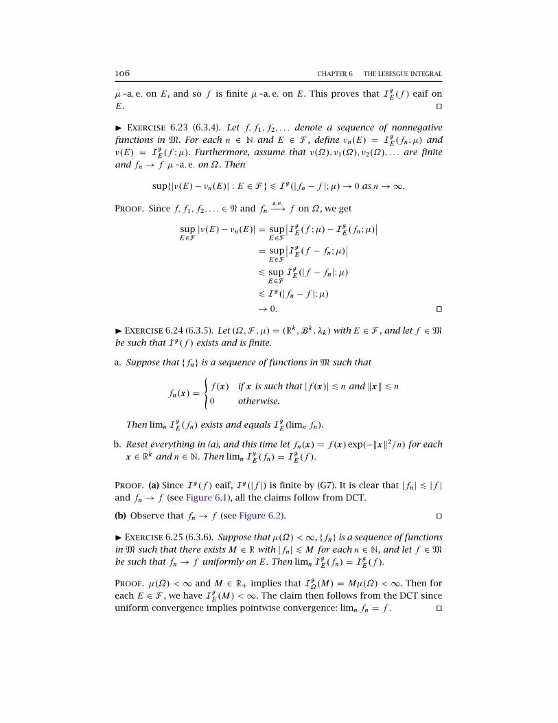
106 CHAPTER 6 THE LEBESGUE INTEGRAL
� –a: e: on E, and so f is finite � –a: e: on E. This proves that g
E .f / eaif on
E. ut
I Exercise 6.23 (6.3.4). Let f; f1; f2; : : : denote a sequence of nonnegative
functions in M. For each n 2 N and E 2 F , define �n.E/ D g
E .fnI�/ and
�.E/ D g
E .f I�/. Furthermore, assume that �.˝/; �1.˝/; �2.˝/; : : : are finite
and fn ! f � –a: e: on ˝. Then
supfj�.E/ � �n.E/j W E 2 F g 6 g.jfn � f jI�/! 0 as n!1:
Proof. Since f; f1; f2; : : : 2 N and fna:e:��! f on ˝, we get
supE2F
j�.E/ � �n.E/j D supE2F
ˇ̌
g
E .f I�/ � g
E .fnI�/ˇ̌
D supE2F
ˇ̌
g
E .f � fnI�/ˇ̌
6 supE2F
g
E .jf � fnjI�/
6 g.jfn � f jI�/
! 0: ut
I Exercise 6.24 (6.3.5). Let .˝;F ; �/ D .Rk ;Bk ; �k/ with E 2 F , and let f 2M
be such that g.f / exists and is finite.
a. Suppose that ffng is a sequence of functions in M such that
fn.x/ D
˚f .x/ if x is such that jf .x/j 6 n and kxk 6 n0 otherwise.
Then limn g
E .fn/ exists and equals g
E .limn fn/.
b. Reset everything in (a), and this time let fn.x/ D f .x/ exp.�kxk2=n/ for each
x 2 Rk and n 2 N. Then limn g
E .fn/ D g
E .f /.
Proof. (a) Since g.f / eaif, g.jf j/ is finite by (G7). It is clear that jfnj 6 jf jand fn ! f (see Figure 6.1), all the claims follow from DCT.
(b) Observe that fn ! f (see Figure 6.2). ut
I Exercise 6.25 (6.3.6). Suppose that �.˝/ <1, ffng is a sequence of functions
in M such that there exists M 2 R with jfnj 6 M for each n 2 N, and let f 2M
be such that fn ! f uniformly on E. Then limn g
E .fn/ D g
E .f /.
Proof. �.˝/ < 1 and M 2 RC implies that g
˝.M/ D M�.˝/ < 1. Then for
each E 2 F , we have g
E .M/ <1. The claim then follows from the DCT since
uniform convergence implies pointwise convergence: limn fn D f . ut
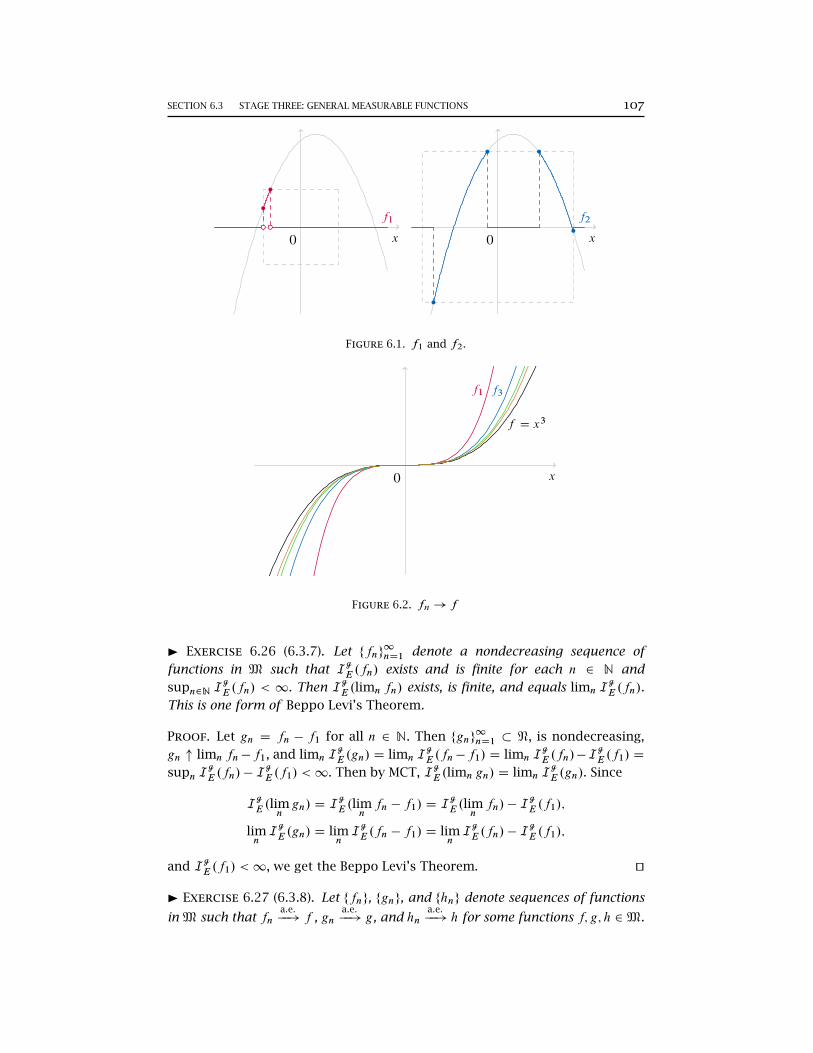
SECTION 6.3 STAGE THREE: GENERAL MEASURABLE FUNCTIONS 107
0 x
f1
0 x
f2
Figure 6.1. f1 and f2.
0 x
f D x3
f1 f3
Figure 6.2. fn! f
I Exercise 6.26 (6.3.7). Let ffng1nD1 denote a nondecreasing sequence of
functions in M such that g
E .fn/ exists and is finite for each n 2 N and
supn2N g
E .fn/ < 1. Then g
E .limn fn/ exists, is finite, and equals limn g
E .fn/.
This is one form of Beppo Levi’s Theorem.
Proof. Let gn D fn � f1 for all n 2 N. Then fgng1nD1 � N, is nondecreasing,
gn " limn fn�f1, and limn g
E .gn/ D limn g
E .fn�f1/ D limn g
E .fn/�g
E .f1/ D
supn g
E .fn/ � g
E .f1/ <1. Then by MCT, g
E .limn gn/ D limn g
E .gn/. Since
g
E .limngn/ D
g
E .limnfn � f1/ D
g
E .limnfn/ �
g
E .f1/;
limn
g
E .gn/ D limn
g
E .fn � f1/ D limn
g
E .fn/ � g
E .f1/;
and g
E .f1/ <1, we get the Beppo Levi’s Theorem. ut
I Exercise 6.27 (6.3.8). Let ffng, fgng, and fhng denote sequences of functions
in M such that fna:e:��! f , gn
a:e:��! g, and hn
a:e:��! h for some functions f; g; h 2M.
108 CHAPTER 6 THE LEBESGUE INTEGRAL
Suppose for any p 2 fg; g1; g2; : : : ; h; h1; h2; : : :g that g
E .p/ exists and is finite.
Furthermore, suppose that limn g
E .gn/ D g
E .g/ and limn g
E .hn/ D g
E .h/. Also,
assume that gn 6 fn 6 hn for every n 2 N.
a. g
E .fn/ exists and is finite for all n 2 N, g
E .f / exists and is finite, and
limn g
E .fn/ D g
E .f /.
b. DCT may be obtained from (a).
Proof. (a) Since fn 6 hn and g
E .hn/ < 1, we have g
E .fn/ 6 g
E .hn/ < 1 for
all n 2 N; that is, g
E .fn/ exists and is finite for all n 2 N.
Since fn 6 hn for all n, we get limn fn 6 limn hn, i.e., f 6 h; since g
E .h/ <1,
we have g
E .f / exists and is finite.
Since fn 6 hn for all n, we have hn � fn > 0 � –a: e:. Fatou’s Lemma yields
g
E .h/ � g
E .f / D g
E .h � f / D g
E .limn.hn � fn//
D g
E .lim infn
.hn � fn//
6 lim infn
g
E .hn � fn/
D lim infn
�
g
E .hn/ � g
E .fn/�
D g
E .h/C lim infn
��
g
E .fn/�I
that is, g
E .f / > lim sup g
E .fn/.
Finally, observe that gn 6 fn yields fn � gn > 0 � –a: e:. Applying Fatou’s
Lemma once again, we obtain
g
E .f / � g
E .g/ D g
E .f � g/ D g
E .limn.fn � gn//
D g
E .lim infn
.fn � gn//
6 lim infn
g
E .fn � gn/
D lim infn
g
E .fn/ � g
E .g/I
that is, g
E .fn/ 6 lim infn g
E .fn/. We thus get limn g
E .fn/ D g
E .f /.
(b) Observe that if jf j 6 g, then �g 6 f 6 g. By (a) we get DCT. ut
I Exercise 6.28 (6.3.12). Suppose that gS1nD1En
.f / exists and is finite, where
fEng1nD1 is a disjoint sequence of F -sets. Then
gS1nD1En
.f / DP1nD1
g
En.f /, and
the convergence of the series is absolute.
Proof. Since gS1nD1En
.f / eaif, (G1-b) implies that each of g
En.f / eaif. There-
fore, gS1nD1En
.f C/;gS1nD1En
.f �/;g
En.f C/;
g
En.f �/ <1. We have
SECTION 6.4 STAGE FOUR: ALMOST EVERYWHERE DEFINED FUNCTIONS 109
gS1nD1En
.f / D gS1nD1En
.f C/ � gS1nD1En
.f �/
D
1XnD1
nEn.f C/ �
1XnD1
nEn.f �/
D
1XnD1
hnEn.f C/ � n
En.f �/
iD
1XnD1
g
En.f /:
We now show thatP1nD1 j
g
En.f /j converges. Since
g
En.f / exists (and is
finite), by (G7) we have jg
En.f /j 6
g
En.jf j/ for any n 2 N; since
g
En.f / eaif
for any n 2 N, we know that g
En.jf j/ eaif for any n 2 N. Therefore,
1XnD1
ˇ̌̌
g
En.f /
ˇ̌̌61XnD1
g
En.jf j/ D
gS1nD1En
.jf j/ <1
since gS1nD1En
.f / eaif. ut
I Exercise 6.29 (6.3.14). Suppose that ffng1nD1 is a sequence of elements of N
converging to some f 2 N. Furthermore, assume that there is 0 6 M <1 such
that g.fn/ 6 M for each n 2 N. Then g.f / exists, is finite, and is no more
than M .
Proof. Let fn ! f . Then limn fn D lim infn fn. By Fatou’s Lemma,
g.f / D g.lim infn
fn/ 6 lim infn
g.fn/ 6 lim supn
g.fn/ 6M: ut
6.4 Stage Four: Almost Everywhere Defined Functions
I Exercise 6.30 (6.4.1). (L10) If f 2 L1.E/ and jgj 6 f � –a: e: on E, then
g 2 L1.E/. Also, any f that is bounded � –a: e: on a set E with �.E/ <1 and
is zero � –a: e: on Ec is in L1.E/.
(L16) We have the following, where A0 2 F 0:
a. If ' > 0, thenRf �1.A0/
' B f d� DRA0' d
�� B f �1
�.
b. For general ',Rf �1.A0/
' B f d� exists and is finite iffRA0' d
�� B f �1
�exists
and is finite, and in this case equality obtains.
Proof. We first prove (L10). f 2 L1.E/ () g
E .f�/ < 1; since jgj 6 f
� –a: e:, we have g�C 6 f � � –a: e: and g�� 6 f � � –a: e:. Then the conclusion
follows (G9). ut

7INTEGRALS RELATIVE TO LEBESGUE MEASURE
7.1 Semicontinuity
I Exercise 7.1 (7.1.1). (SC4b) If f .x/ D �1, then f is USC at x iff limy!x f .y/ D
�1.
(SC7b) xf is USC, and is the minimal USC function > f .
(SC9) Let A denote a generic nonempty index set. For each ˛ 2 A, suppose that
f˛ is a function from Rk into xR. We have the following:
a. If f˛ is LSC for each ˛ 2 A, then sup˛2A f˛ is LSC.
b. If f˛ is USC for each ˛ 2 A, then inf˛2A f˛ is USC.
Proof. (SC4b) Assume f is USC at x. Pick t > f .x/ D �1. Then there is
ı > 0 such that f .y/ < t for each y 2 B .x; ı/. Since t is arbitrary, we
have limy!x f .y/ D �1. Conversely, assume that limy!x f .y/ D �1 and
pick any t > f .x/ D �1. Then there is ı > 0 such that f .y/ < t for each
y 2 B .x; ı/. Since t is generic, f is USC at x by definition.
(SC7b) We show that infı>0 supy2B.x;ı/ xf .y/ 6 xf .x/ for each x; then xf is
USC by (SC6). Suppose there is x so that the preceding inequality fails, then
there exists t such that infı>0 supy2B.x;ı/ xf .y/ > t > xf .x/. It follows that
supy2B.x;ı/ xf .y/ > t for any ı > 0, and therefore, there exists y 2 B .x; ı/
so that xf .y/ > t for any B .x; ı/. Now consider an open ball of y , B .y; r/ �
B .x; ı/. We have
xf .y/ D infı0>0
supz2B.y;ı0/
f .z/ 6 supz2B.y;r/
f .z/ 6 supz2B.x;ı/
f .z/;
that is, for any B .x; ı/, we have supz2B.x;ı/ f .z/ > xf .y/ > t . But this implies
thatxf .x/ D inf
ı>0sup
z2B.x;ı/
f .z/ > t:
A contradiction.
111
112 CHAPTER 7 INTEGRALS RELATIVE TO LEBESGUE MEASURE
With this outcome, we can show that f is LSC. Take any x 2 Df . Then
�f .x/ D infı>0
supy2B.x;ı/
��f
�.y/ D � sup
ı>0
infy2B.x;ı/
f .y/ D �f .x/:
Since �f is USC, �.�f / is LSC, that is, f D �.�f / D �.�f / is LSC.
(SC9a) Take any x 2 xRk and t < sup˛2A f˛.x/. Then there exists ˛0 2 A such
that f˛0.x/ > t ; since f˛0 is LSC, there is B .x; ı/ such that f˛0.y/ > t for all
y 2 B .x; ı/. Since sup˛2A f˛.y/ > f˛0.y/, we know that sup˛2A f˛ is LSC.
(SC9b) f˛ is USC implies that �f˛ is LSC; then sup˛2A.�f˛/ D � inf˛2A f˛ is
LSC. Hence, inf˛2A f˛ is USC.
ut
I Exercise 7.2 (7.1.2). Let E � xRk .
a. E is open iff 1E is LSC.
b. E is closed iff 1E is USC.
c. We have 1E D 1Eı and 1E D 1E .
Proof. ut
8THE LP SPACES
8.1 Lp Space: The Case 1 6 p < C1
I Exercise 8.1 (8.1.1). Pick A;B 2 Lp . Then A C B 2 Lp and kA C Bkp 6kAkp C kBkp .
Proof. Let h 2 ACB, so that h D f C g for some f 2 A and g 2 B. NowZjhjp D
�Zjf C gjp
�p=p6
"�Zjf jp
�1=pC
�Zjgjp
�1=p#p< C1
by Minkowski’s Inequality, and hence A C B 2 Lp . The above display also
implies that
kACBkpp 6�kAkp C kBkp
�p;
i.e., kACBkp 6 kAkp C kBkp . ut
I Exercise 8.2 (8.1.2). Prove the Cauchy-Schwarz inequalityˇ̌̌̌ˇ̌ nXkD1
akbk
ˇ̌̌̌ˇ̌ 6p
kXkD1
a2k
pnXkD1
b2k :
Proof. Let p D p0 D 2; then Hölder’s Inequality becomesˇ̌̌̌Zfg
ˇ̌̌̌6 kf k2 � kgk2: (8.1)
Let ˝ D f!1; : : : ; !ng, F D 2˝ , � be the counting measure, f .!i / D ai , and
g .!i / D bi . Then jRfgj D j
P!i2˝
f .!i / g .!i / j D jPnkD1 akbkj,
kf k2 D
�Zjf j2
�1=2D
0@X!i2˝
jf .!i /j2
1A1=2 Dp
nXkD1
a2k ;
113
114 CHAPTER 8 THE LP SPACES
and similarly for kgk2. Put these into (8.1) and we get the Cauchy-Schwarz
inequality. See Shirali and Vasudeva (2006, Theorem 1.1.4) for a direct proof.
ut
I Exercise 8.3 (8.1.3). Let 1 < p1; : : : ; pn < C1 be such that 1=p1C� � �C1=pn D
1, and pick functions f1 2 Lp1 ; : : : ; fn 2 Lpn . We wish to generalize Hölder’s
Inequality by showing thatQniD1 fi 2 L
1 and jR Qn
iD1 fi j 6QniD1 kfikpi .
a. Show first that a1 � � � an 6 ap11 =p1 C � � � C apnn =pn by generalizing the calculus
result given in the section. [Here 0 6 a1; : : : ; an < C1.]
b. If kf1kp1 D 0 or : : : or kfnkpn D 0, the claim is trivial.
c. Use (a) to prove the claim when kf1kp1 D � � � D kfnkpn D 1.
d. Prove the claim when kf1kp1 ; : : : ; kfnkpn are positive.
Proof. (a) This is the arithmetic mean-geometric mean inequality, or AM-GM
inequality, for short. Since ln is concave, we have
nXiD1
1
piln xi 6 ln
0@ nXiD1
1
pixi
1A ;i.e.,
ln
0@ nYiD1
x1=pii
1A 6 ln
0@ nXiD1
xi
pi
1A () nYiD1
x1=pii 6
nXiD1
xi
pi:
Let x1=pii D ai , then xi D apii and we have the desired result.
(b) Let kfikpi D 0; then fi D 0 � –a: e: on ˝. But thenQniD1 fi D 0 � –a: e: on ˝,
henceQniD1 fi 2 L
1 and the desired inequality in this case is actually the trivial
equation 0 D 0.
(c) If kf1kp1 D � � � D kfnkpn D 1, observe thatˇ̌̌̌ˇ̌ nYiD1
fi .!/
ˇ̌̌̌ˇ̌ D nY
iD1
jfi .!/j 6nXiD1
1
pijfi .!/j
pi 8 ! 2 ˝;
by the Am-GM inequality. Therefore,Z ˇ̌̌Yn
iD1fi
ˇ̌̌6
nXiD1
1
pi
Zjfi j
pi D
nXiD1
1
pikfikpi D 1:
This shows thatQniD1 fi 2 L
1.
(d) Define f �i D fi=kfikpi for any i D 1; : : : ; n. We have
�Z ˇ̌f �iˇ̌pi�1=pi
D
�Z ˇ̌fi=kfikpi
ˇ̌pi�1=piD
1
kfikpipi
Zjfi j
pi
!1=piD 1;
SECTION 8.1 LP SPACE: THE CASE 1 6 P < C1 115
which shows that f �i 2 Lpi and kf �i kpi D 1. By (c),QniD1 f
�i 2 L1 andR
jQniD1 f
�i j 6 1. Since
QniD1 fi D
�QniD1 kfikpi
� �QniD1 f
�i
�, we have
Z ˇ̌̌̌ˇ̌ nYiD1
fi
ˇ̌̌̌ˇ̌ D
0@ nYiD1
kfikpi
1AZ ˇ̌̌̌ˇ̌ nYiD1
f �i
ˇ̌̌̌ˇ̌ 6 nY
iD1
kfikpi < C1;
givingQniD1 fi 2 L
1, andˇ̌̌̌ˇ̌Z nY
iD1
fi
ˇ̌̌̌ˇ̌ 6 Z
ˇ̌̌̌ˇ̌ nYiD1
fi
ˇ̌̌̌ˇ̌ D
nYiD1
fi
1
6nYiD1
kfikpi : ut
I Exercise 8.4 (8.1.4). We have equality in Hölder’s Inequality iff there are
nonnegative numbers A and B , not both zero, with Ajf jp D Bjgjp0
� –a: e: on
˝.
Proof. We have equality in Hölder’s Inequality iff
jf j
kf kp�jgj
kgkp0D1
p
jf jp
kf kppC1
p0jgjp
0
kgkp0
p0
� –a: e: on ˝;
which holds iff the AM-GM holds equality, that is,
jf jp
kf kppDjgjp
0
kgkp0
p0
�-a.e. on ˝: ut
I Exercise 8.5 (8.1.5). Given f 2 Lp�1 < p < C1
�, there is g 2 Lp
0
with
kgkp0 D 1 andRfg D kf kp .
Proof. Let g D .f = kf kp/p�1. Then
Zjgjp
0
D
Z ˇ̌̌̌ˇ̌
f
kf kp
!p�1 ˇ̌̌̌ˇ̌p0
D
Z ˇ̌̌̌ˇ f
kf kp
ˇ̌̌̌ˇp
D1
kf kpp
Zjf jp D
kf kpp
kf kppD 1;
i.e., kgkp0 D 1. We also haveZjfgj D
Zjf jp
kf kp�1p
D kf kp : ut
I Exercise 8.6 (8.1.6). We now explore conditions for equality in Minkowski’s
Inequality. Let f; g 2 Lp .
a. When p D 1, kf C gkp D kf kp C kgkp iff there exists positive F =B�-
measurable h > 0 defined on ˝ with f h D g � –a: e: on f! 2 ˝ W f .!/g.!/ ¤
0g.
b. For 1 < p < C1, equality obtains iff there are nonnegative real numbers A
and B , not both zero, such that Af D Bg � –a: e: on ˝.
116 CHAPTER 8 THE LP SPACES
Proof. (a) When p D 1, we have
kf C gk1 D kf k1 C kgk1 ()
Zjf C gj D
Zjf j C
Zjgj
()
Z �jf C gj � jf j � jgj
�D 0
() jf C gj D jf j C jgj � –a: e:
() 9F =B�-measurable h > 0 defined on ˝
with f h D g � –a: e: on Œf .!/g.!/ ¤ 0�.
(b) When 1 < p <1, we have
kf C gkpp D
Zjf C gjp
D
Zjf C gj � jf C gjp�1
�
6Zjf j � jf C gjp�1 C
Zjgj � jf C gjp�1
��
6 kf kp � kjf C gjp�1kp0 C kgkp � kjf C gjp�1kp0
D�kf kp C kgkp
�kf C gkp�1p :
Hence, the Minkowski’s Inequality holds with equality iff .�/ and .��/ hold with
equality. The result follows from Exercise 8.4 that .��/ immediately. ut
I Exercise 8.7 (8.1.7). Let 1 6 p; q; r < C1 be such that 1=r D 1=p C 1=q. Let
f 2 Lp and g 2 Lq . Then fg 2 Lr and kfgkr 6 kf kp kgkq .
Proof. Let p0 D p=r and q0 D q=r . Then 1=p0 C 1=q0 D r=p C r=q D 1. Let
f � D f r and g� D gr . ThenZjf �jp
0
D
Zjf r jp=r D
Zjf jp < C1;
and Zjg�jq
0
D
Zjgr jq=r D
Zjgjq < C1;
i.e., f � 2 Lp0
and g� 2 Lq0
. By the AM-GM inequality, for any ! 2 ˝,ˇ̌f �.!/g�.!/
ˇ̌D jf �.!/j � jg�.!/j 6
1
p0jf �.!/jp
0
C1
q0jg�.!/jq
0
:
Integrate the left and right sides of the above display, obtainingZjfgjr D
Zjf �g�j 6
1
p0
Zjf �jp
0
C1
q0
Zjg�jq
0
< C1;
that is, fg 2 Lr and f �g� 2 L1. Then by Hölder’s Inequality, we have
kf �g�k1 6 kf �kp0kg�kq0 I
SECTION 8.2 THE RIESZ-FISCHER THEOREM 117
therefore, Zjfgjr D
Zjf �g�j 6
�Zjf �jp
0
�1=p0 �Zjg�jq
0
�1=q0D
"�Zjf jp
�1=p �Zjgjq
�1=q#rD
�kf kp kgkq
�rI
that is, kfgkr 6 kf kp kgkq . ut
I Exercise 8.8 (8.1.8). If 1 6 p < C1, Minkowski’s Inequality givesˇ̌̌kf kp � kgkp
ˇ̌̌6
kf � gkp for every f; g 2 Lp .
Proof. Write f D�f � g
�C g. We first show that f � g 2 Lp when f; g 2 Lp .Z
jf � gjp 6Zjf jp C
Zjgjp < C1:
Then by the Minkowski’s Inequality, we have
kf kp D k.f � g/C gkp 6 kf � gkp C kgkp:
Rearrange the above display and we get the desired result. ut
8.2 The Riesz-Fischer Theorem
I Exercise 8.9 (8.2.1). Return to the formal definition of Lp .
a. Write out the formal definition of convergence in Lp .
b. State and prove the formal version of the Riesz-Fischer Theorem.
Proof. (a) Let F;F1;F2; : : : 2 Lp . fFng
1nD1 converges to F in Lp , Fn
Lp
��! F, if
and only if limn kFn �Fkp D 0.
(b) Straightforward. ut
I Exercise 8.10 (8.2.2). Let .X; �/ denote a generic metric space. Let Cb.X/
denote the collection of continuous real-valued bounded functions on X . For
f 2 Cb.X/, write kf k D supx2X jf .x/j, the usual supremum norm. Then Cb.X/
is a Banach space.
Proof. Let ffng be a Cauchy sequence in Cb.X/. Then for every " > 0, there
exists N" 2 N such that for all n;m > N", we have
kfn � fmk D supx2X
jfn.x/ � fm.x/j < ":
118 CHAPTER 8 THE LP SPACES
Therefore, for every x 2 X , we get jfn.x/ � fm.x/j < " for all n;m > N"; that is,
ffk.x/g is Cauchy in R. The completeness of R yields
fk.x/! f .x/;
for some f .x/ 2 R. Now fix n > N". Since j � j is continuous, we get
jfn.x/ � f .x/j D limm!1
jfn.x/ � fm.x/j 6 ":
Hence, for every n > N", we have
kf � fnk D supx2X
jfn.x/ � f .x/j 6 ":
What has been just shown is that kf � fnk ! 0 as n ! 1. Note that this
implies that fn ! f uniformly on X . Thus, f is continuous since every fn is
continuous. Also,
kf k 6 kf � fnk C kfnk <1:
Hence f 2 Cb.X/ and so Cb.X/ is a Banach space. ut
I Exercise 8.11 (8.2.3). A function f on Rk is said to vanish at infinity iff
f .x/ ! 0 as kxk ! 1. Show that the collection of continuous functions on Rk
that vanish at infinity is a Banach space relative to the supremum norm given
in the previous exercise.
Proof. Let C0.Rk/ denote the collection of continuous functions on Rk that
vanish at infinity. We use an alternative definition (Rudin, 1986, Definition
3.16): A complex function f on a locally compact Hausdorff space X is said to
vanish at infinity if to every " > 0 there exists a compact set K � X such that
jf .x/j < " for all x … K.
Let ffng be a Cauchy sequence in C0.Rk/, i.e., assume that ffng converges
uniformly. Then its pointwise limit function f is continuous. Given " > 0,
there exists an n so that kfn � f k < "=2 and there is a compact set K so that
jfn.x/j < "=2 outside K. Hence jf .x/j < " outside K, and we have proved that
f vanishes at infinity. Thus C0.Rk/ is complete. ut
I Exercise 8.12 (8.2.4). Let Cc.Rk/ denote the collection of continuous functions
on Rk with compact support, and again consider the supremum norm. This
collection is dense in the collection in the previous exercise, but it fails to be a
Banach space.
Proof. Refer Hewitt and Stromberg (1965, §7) and Rudin (1986, p. 69-71). The
support of a (complex) function f on a topological space X is the closure of
the set fx 2 X W f .x/ ¤ 0g.
Given f 2 C0.Rk/ and " > 0, there is a compact set K so that jf .x/j < "
outside K. Urysohn’s lemma (Rudin, 1986, 2.12) gives us a function g 2 Cc.Rk/
SECTION 8.3 LP SPACE: THE CASE 0 < P < 1 119
such that 0 6 g 6 1 and g.x/ D 1 on K. Put h D fg. Then h 2 Cc.Rk/ and
kf � hk < ". This proves that Cc.Rk/ D C0.Rk/. ut
I Exercise 8.13 (8.2.5). A sequence ffng in Lp may converge in pth mean to
some f 2 Lp but at the same time fail to converge pointwise to f at any point in
˝. Therefore, convergence in Lp does not in general imply convergence � –a: e:
Proof. Consider .Œ0; 1�;BŒ0; 1�; �/. Consider the sequence
1Œ0;1=2�; 1Œ1=2;1�; 1Œ0;1=4�; 1Œ1=4;1=2�; 1Œ1=2;3=4�; 1Œ3=4;1�; 1Œ0;1=8�; : : : :
Then fnLp
��! 0, but obviously f .x/ 6! 0 for all x 2 Œ0; 1�. ut
8.3 Lp Space: The Case 0 < p < 1
I Exercise 8.14 (8.3.1). Let f; g 2 Lp , where 0 < p < 1. We know that f C g 2
Lp by the Minkowski-like Inequality result given earlier.
a. We have .aC b/p 6 ap C bp for every 0 < a; b <1.
b. From (a), we haveRjf C gjp 6
Rjf jp C
Rjgjp .
c. If we write kf � gkpp for the distance between f and g, then this distance
function is truly a metric, if we identify functions equal � –a: e: on ˝.
d. Writing kf � gkp for the distance between f and g does not define a metric
on Lp .
Proof. (a) If 0 < a D b <1, we have
.aC b/p D 2pap 6 2ap D ap C bp:
Next we assume that 0 < a < b < 1. Since 0 < p < 1, the function xp defined
on .0;1/ is concave. Write b as a convex combination of a and aCb as follows:
b Da
baC
b � a
b.aC b/:
Then
bp D
�a
baC
b � a
b.aC b/
�p6a
bap C
b � a
b.aC b/pI
that is,
.aC b/p 6bpC1 � apC1
b � a6.b � a/.ap C bp/
b � aD ap C bp;
where the second inequality holds since
.b � a/.ap C bp/ D bpC1 � apC1 C ab�ap�1 � bp�1
�> bpC1 � apC1:
120 CHAPTER 8 THE LP SPACES
(b) It follows from (a) thatZjf C gjp 6
Z.jf j C jgj/p 6
Z.jf jp C jgjp/ D
Zjf jp C
Zjgjp:
(c) We use the informal definition. To see kf � gkpp is a metric on Lp , we need
to verify:
� 0 6 kf � gkpp <1 for every f; g 2 Lp . It is true because by (b):
0 6 kf � gkpp DZjf � gjp 6
Zjf jp C
Zjgjp <1:
� kf � f kpp D 0 for each f 2 Lp , and kf � gkpp D 0 forces f D g � –a: e: on
˝. The first claim is obvious, so we focus on the second one. If kf � gkpp DRjf � gjp D 0, then jf � gjp D 0 � –a: e:, then f D g � –a: e:
� kf � gkpp D kg � f k
pp for every f; g 2 Lp . This is evident.
� kf � hkpp 6 kf � gkpp C kg � hkpp for every f; g; h 2 Lp . It also follows from
(b):
kf � hkpp D
Zjf � hjp D
Zj.f � g/C .g � h/jp
6Z.jf � gj C jg � hj/p
6Zjf � gjp C
Zjg � hjp
D kf � gkpp C kg � hkpp :
Thus, kf � gkpp is a metric on Lp when 0 < p < 1.
(d) It follows from the Minkowski-like equality that the triangle inequality fails
for kf � gkp when 0 < p < 1. ut
I Exercise 8.15 (8.3.2). Consider the space ˝ D .0; 1/ and let 0 < p < 1. Write
B for the Borel subsets of .0; 1/, and write � for Lebesgue measure restricted to
B. We will show that there exists no norm k k on Lp such that limk kfkkp D 0
forces limk kfkk D 0.
a. Suppose that such a norm k k exists. Then there is C > 0 such that kf k 6Ckf kp for each f 2 Lp .
Pick the minimal such C from (a).
b. There is 0 < c < 1 withR c0jf jp D
R 1cjf jp D 1
2
R 10jf jp .
c. Let g D f 1.0;c� and h D f 1.c;1�, so that f D g C h. Then kgkp D khkp D
2�1=pkf kp and kf k 6 kgkCkhk 6 CkgkpCCkhkp D C � 21�1=pkf kp . Use the
minimality of C to obtain C 6 C21�1=p , and deduce C D 0.
SECTION 8.3 LP SPACE: THE CASE 0 < P < 1 121
d. Conclude that kf k D 0 for every f 2 Lp , and hence the assumption in (a)
entails a contradiction.
Proof. (a) Suppose that for every C > 0 there is f 2 Lp with kf k > Ckf kp .
Then for every k 2 N there is fk 2 Lp with kfkk > kkfkkp . Define gk D fk=kfkk
for each k 2 N. Then kgkk D 1 and for every k 2 N
1 D kgkk > kkgkkp;
i.e., kgkk < 1=k. Hence, limk kgkkp D 0, so limk kgkk D 0 by the assumption
that such a norm exists. But limk kgkk D 1.
(b) The functionR x0jf jp is continuous and increasing with respect to x. The
claim follows immediately.
(c) It follows from (b) that kgkpp D khkpp D
12kf kp , i.e.,
kgkp D khkp D 2�1=pkf kp:
Since k k is a norm, we have
kf k D kg C hk 6 kgk C khk 6 Ckgkp C Ckhkp D C21�1=pkf kp:
The minimality of C implies that C 6 C21�1=p . Hence, C D 0.
(d) By (a) and (c) we get kf k 6 0kf kp D 0; that is, kf k D 0 for all f 2 Lp . But
then k k is not a norm. A contradiction. ut
I Exercise 8.16 (8.3.3). Let 0 < p0 < 1 and let f 2 Lp0 be nonnegative. Let
E1 D f! 2 ˝ W f .!/ D 0g, E2 D f! 2 ˝ W 0 < f .!/ 6 1g, and E3 D f! 2 ˝ W
f .!/ > 1g.
a. limp!0C
RE2jf jp D �.E2/.
b. limp!0C
RE3jf jp D �.E3/.
c. limp!0C
Rjf jp D �.f! 2 ˝ W f .!/ ¤ 0g/.
Proof. (a) The function xp decreasing with respect to p when 0 < x 6 1. By
MCT we have
limp!0C
ZE2
jf jp D
ZE2
limp!0C
jf jp D
ZE2
1 D �.E2/:
(b) It follows from DCT.
(c) Let fpng be a decreasing sequence converging to 0. Then
limn
Zjf jp D lim
n
ZE2
jf jp C
ZE3
jf jp
!D lim
n
ZE2
jf jp C limn
ZE3
jf jp
D �.E2/C �.E3/
D �Œf .!/ ¤ 0�: ut
122 CHAPTER 8 THE LP SPACES
I Exercise 8.17 (8.3.4). Say �.˝/ D 1, and let f 2 L1 be nonnegative. Write
log 0 D �1.
a.R
logf 6 logRf if logf 2 L1.
b. If logf … L1, thenR.logf /C < 1 under the assumption f 2 L1, so it must
be the case thatR.logf /� D 1. Conclude that even if logf … L1,
Rlogf
still exists and equals �1, giving the inequality in (a).
c. .f r�1/=r decreases to logf as r ! 0C, hence limr!0C.Rf r�1/=r D
Rlogf .
d. Verify the inequalities
1
r
�Zf r � 1
�>1
rlog
Zf r >
1
r
Zlogf r D
Zlogf:
e. Conclude that limr!0C kf kr exists and equals exp.R
logf /. If logf … L1, this
is interpreted as limr!0C kf kr D 0.
Proof. (a) If kf k1 DRf D 0, then f D 0 � –a: e:. Hence,
Rlogf D log
Rf D
�1. Now assume that kf k1 > 0. Since log x 6 x � 1 when 0 6 x <1, we haveZlog
f
kf k16Z �
f
kf k1� 1
�D
Rf
kf k1�
Z1 D 0I
hence, Zlogf 6 log kf k1 D log
Zf:
(b) Observe that
.logf /C.!/ D
˚0 if f .!/ 2 Œ0; 1�
logf .!/ if f .!/ 2 .1;1�:
Also, logf .!/ < f .!/ � 1 when ! 2 .1;1�. Since f 2 L1, we haveRf < 1.
Thus, Z.logf /C D
ZŒf .!/>1�
logf 6ZŒf .!/�>1
.f � 1/ <1:
Therefore, it must be the case thatR.logf /� D1, and soZ
logf D
Z.logf /C �
Z.logf /� D �1:
(c) Fix an arbitrary ! 2 ˝. We have
limr!0C
f .!/r � 1
rD logf .!/I
hence, .f r � 1/=r # logf as r ! 0C, and consequently,�f �
f r � 1
r
�"�f � logf
�as r ! 0C:
SECTION 8.4 LP SPACE: THE CASE P D C1 123
It follows from the MCT that
limr!0C
Z �f �
f r � 1
r
�D
Zf � lim
r!0C
Zf r � 1
r
D
Zf �
Zlimr!0C
f r � 1
r
D
Zf �
Zlogf:
SinceRf <1 and �.˝/ D 1, we get the desired result.
(d) The first inequality follows from the fact f r > 0 and under this case
logf r 6 f r � 1. The second inequality follows from (a) and (b).
(e) ut
8.4 Lp Space: The Case p D C1
I Exercise 8.18 (8.4.2). Consider the � -finite measure space .˝;F ; �/.
a. f 2 L1 iff there is a bounded F =B�-measurable function g on ˝ such that
f D g � –a: e: on ˝.
b. If f 2 L1, then kf k1 D inffsup!2˝ jg.!/j W g is as in (a)g.
Proof. (a) First assume that there exists a bounded F =B�-measurable func-
tion g on˝ such that f D g � –a: e:. Then there existsM > 0 such that jgj 6M .
Hence, jf j 6M � –a: e:; that is, ess supf 6M , and so f 2 L1.
Now suppose that f 2 L1. Define g on ˝ by letting
g.!/ D
˚f .!/ if jf .!/j 6 ess supf
0 otherwise:
This g is bounded, F =B�-measurable, and f D g � –a: e:.
(b) We first show that sup!2˝ jg.!/j > kf k1 for all g as in (a). Suppose that
sup!2˝ jg.!/j < kf k1. Define
A´
(! 2 ˝ W jf .!/j > sup
!2˝
jg.!/j
):
Then �.A/ > 0; for otherwise kf k1 6 sup!2˝ jg.!/j. But which means that
f > g on A and �.A/ > 0. A contradiction. This shows that
inf
(sup!2˝
jg.!/j W g as in (a)
)> kf k1:
124 CHAPTER 8 THE LP SPACES
We next show the reverse inclusion. Let B ´ f! 2 ˝ W jf .!/j 6 kf k1g; then
�.Bc/ D 0. Let g D f 1B . Then g is bounded, F =B�-measurable, and f D g
� –a: e:. Furthermore,
sup!2˝
j.f 1B/.!/j 6 kf k1:
This prove that kf k1 2 fsup!2˝ W jg.!/j W g as in (a)g, and the proof is com-
pleted. ut
I Exercise 8.19 (8.4.4). Quickly prove the p D1 version of Hölder’s Inequality.
Proof. Let f 2 L1 and g 2 L1. By Claim 1 we get
jfgj 6 ess supfg � –a: e:
Observe that
ess supfg D jgjess supf D jgj � kf k1;
so we have Zjfgj 6
Zjgj � kf k1 D kf k1kgk1 <1:
Hence, fg 2 L1 and kfgk1 6 kf k1kgk1. ut
I Exercise 8.20 (8.4.5). Let .˝;F ; �/ be such that �.˝/ <1, and let f denote
a bounded F =B�-measurable function on ˝.
a. For every 1 6 p 61 we have f 2 Lp , hence kf kp exists.
b. limp!1 kf kp D kf k1.
Proof. (a) Since f is bounded, there exists 0 6 M 6 1 such that jf j 6 M .
Then ess supf 6M ; that is, kf k1 exists. Now consider 1 6 p <1. We haveZjf jp 6
ZMpDMp�.˝/ <1;
i.e., kf kp exists.
(b) If f D 0 � –a: e:, then kf kp D kf k1 D 0 for all p, and the claim is trivial.
So assume that f ¤ 0 on a set of positive measure, so that kf k1 > 0. We
first show that lim infp!1 kf kp > kf k1. Let t 2 .0; kf k1/. By the Chebyshev’s
Inequality (Exercise 8.24) we have
kf kp > t�Œjf .!/j > t �1=p:
If �Œjf .!/j > t � D1, the claim is trivial. If �Œjf .!/j > t � <1, then
lim infp!1
kf kp > lim infp!1
t�Œjf .!/j > t �1=p D limp!1
t�Œjf .!/j > t �1=p D t:
Since t 2 .0; kf k1/ is arbitrary, we have limp!1 kf kp > kf k1.
We next show that lim supp!1 kf kp 6 kf k1. It follows from (a) that kf k1exists, and so jf j 6 kf k1 � –a: e:. Then
SECTION 8.5 CONTAINMENT RELATIONS FOR LP SPACES 125
kf kpp D
Zjf jp 6
Zkf kp1 D kf k
p1�.˝/I
that is, kf kp 6 kf k1�.˝/1=p . Then
lim supp!1
kf kp 6 kf k1:
Summarizing the findings, we have limp!1 kf kp D kf k1. ut
8.5 Containment Relations for Lp Spaces
I Exercise 8.21 (8.5.1). Consider the measure space .R;B; �/. Let 1 6 p < q <1, and let r be such that 1=q < r < 1=p.
a. Define f on R by writing f .x/ D x�r1.0;1/.x/ for each x 2 R. Then f 2 Lp
but f … Lq . Therefore, we do not in general have Lp � Lq when p < q.
b. Let g.x/ D x�r1.1;1/.x/ for every x 2 R. Then g 2 Lq but g … Lp . Therefore,
we do not in general have Lq � Lp when p < q.
Proof. (a) We have �rq < �1 < �rp. Hence,
Zjf jp D
Z.0;1/
x�rp Dx1�rp
1 � rp
ˇ̌̌̌ˇ1
0
D1
1 � rp<1;
Zjf jq D
Z.0;1/
x�rq Dx1�rq
1 � rq
ˇ̌̌̌ˇ1
0
D1I
that is, f 2 Lp , but f … Lq .
(b) We have Zjgjq D
Z.1;1/
x�rq Dx1�rq
1 � rq
ˇ̌̌̌ˇ1
1
D1
rq � 1<1;
Zjgjp D
Z.1;1/
x�rp Dx1�rp
1 � rq
ˇ̌̌̌ˇ1
1
D1I
hence, g 2 Lq but g … Lp . ut
Remark 8.22 (Folland 1999, p.185). Thus we see two reasons why a function
f may fail to be in Lp : either jf jp blows up too rapidly near some point, or it
fails to decay sufficiently rapidly at infinity. In the first situation the behavior
of jf jp becomes worse as p increases, while in the second it becomes better.
In other words, if p < q, functions in Lp can be locally more singular than
functions in Lq , whereas functions in Lq can be globally more spread out than
functions in Lp . See Figure 8.1.
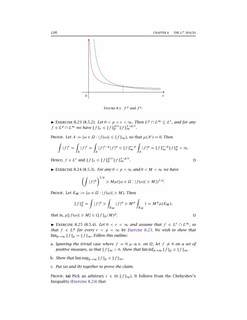
126 CHAPTER 8 THE LP SPACES
0 x
Figure 8.1. f p and f q .
I Exercise 8.23 (8.5.2). Let 0 < p < r < 1. Then Lp \ L1 � Lr , and for any
f 2 Lp \ L1 we have kf kr 6 kf kp=rp kf k1�p=r1 .
Proof. Let A´ f! 2 ˝ W jf .!/j 6 kf k1g, so that �.Ac/ D 0. ThenZjf jr D
ZA
jf jr D
ZA
jf jr�pjf jp 6 kf kr�p1ZA
jf jp D kf kr�p1 kf kpp <1:
Hence, f 2 Lr and kf kr 6 kf kp=rp kf k1�p=r1 . ut
I Exercise 8.24 (8.5.3). For any 0 < p <1 and 0 < M <1 we have�Zjf jp
�1=p>M�.f! 2 ˝ W jf .!/j >M g/1=p:
Proof. Let EM ´ f! 2 ˝ W jf .!/j >M g. Then
kf kpp D
Zjf jp >
ZEM
jf jp >Mp
ZEM
1 DMp�.EM /I
that is, �Œjf .!/j >M� 6 .kf kp=M/p . ut
I Exercise 8.25 (8.5.4). Let 0 < r < 1 and assume that f 2 Lr \ L1, so
that f 2 Lp for every r < p < 1 by Exercise 8.23. We wish to show that
limp!1 kf kp D kf k1. Follow this outline:
a. Ignoring the trivial case where f D 0 � –a: e: on ˝, let f ¤ 0 on a set of
positive measure, so that kf k1 > 0. Show that lim infp!1 kf kp > kf k1.
b. Show that lim supp!1 kf kp 6 kf k1.
c. Put (a) and (b) together to prove the claim.
Proof. (a) Pick an arbitrary t 2 .0; kf k1/. It follows from the Chebyshev’s
Inequality (Exercise 8.24) that
SECTION 8.7 MORE CONVERGENCE CONCEPTS 127
kf kp > t � �Œjf .!/j > t �1=p:
If �Œjf .!/j > t � D 1, then kf kp D 1 for all p, and the claim is trivial. If
�Œjf .!/j > t � <1, then limp!1 �Œjf .!/j > t �1=p D 1 and so lim infp!1 kf kp >t . Since t 2 .0; kf k1/ is chosen arbitrarily, we get
lim infp!1
kf kp > kf k1 (8.2)
(b) By Exercise 8.23 we have kf kp 6 kf kr=pr kf k1�r=p1 , for every p 2 .r;1/.
Hence,
lim supp!1
kf kp 6 kf k1: (8.3)
(c) Combining (8.2) and (8.3) we get
kf k1 6 lim infp!1
kf kp 6 lim supp!1
kf kp 6 kf k1:
Hence, limp!1 kf kp D kf k1. ut
I Exercise 8.26 (8.5.5). Let �.˝/ D 1 and 1 6 p 6 q 6 1. Show for arbitrary
f that Zjf j 6
�Zjf jp
�1=pD
�Zjf jq
�1=q6 ess supf;
so that kf k1 6 kf kp 6 kf kq 6 kf k1.
Proof. It follows from Claim 1 and the assumption that �.˝/ D 1. ut
8.6 Approximation
8.7 More Convergence Concepts
I Exercise 8.27 (8.7.1). Prove the following simple claims.
a. Let ffng1nD1 denote a Cauchy sequence in Lp , where 0 < p < 1. Show that
ffng1nD1 is a Cauchy sequence in measure: for every " > 0 and ı > 0 there is
N 2 N such that for every n;m > N we have �.f! 2 ˝ W jfn.!/ � fm.!/j >
ıg/ < ".
b. Let f; f1; f2; : : : 2 Lp and suppose that fnLp
��! f , where 0 < p <1. If g 2 L1,
then fg; f1g; f2g; : : : 2 Lp and fngLp
��! fg.
Proof. (a) Choose arbitrary " > 0 and ı > 0. It follows from Chebyshev’s
Inequality that
�Œjfn.!/ � fm.!/j > ı� 6kfn � fmk
pp
ıp:
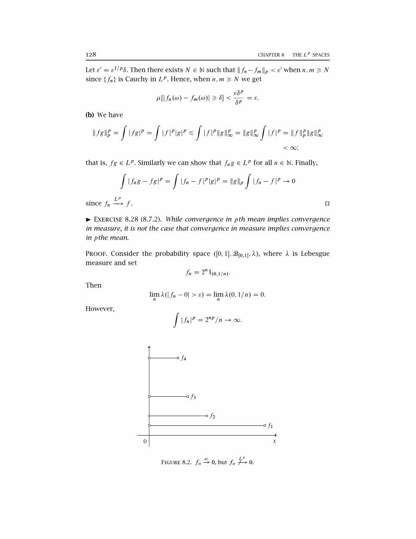
128 CHAPTER 8 THE LP SPACES
Let "0 D "1=pı. Then there exists N 2 N such that kfn�fmkp < "0 when n;m > Nsince ffng is Cauchy in Lp . Hence, when n;m > N we get
�Œjfn.!/ � fm.!/j > ı� <"ıp
ıpD ":
(b) We have
kfgkpp D
Zjfgjp D
Zjf jpjgjp 6
Zjf jpkgkp1 D kgk
p1
Zjf jp D kf kpp kgk
p1
<1I
that is, fg 2 Lp . Similarly we can show that fng 2 Lp for all n 2 N. Finally,Zjfng � fgj
pD
Zjfn � f j
pjgjp D kgkp
Zjfn � f j
p! 0
since fnLp
��! f . ut
I Exercise 8.28 (8.7.2). While convergence in pth mean implies convergence
in measure, it is not the case that convergence in measure implies convergence
in pthe mean.
Proof. Consider the probability space .Œ0; 1�;BŒ0;1�; �/, where � is Lebesgue
measure and set
fn D 2n1.0;1=n/:
Then
limn�.jfn � 0j > "/ D lim
n�.0; 1=n/ D 0:
However, Zjfnj
pD 2np=n!1:
0 x
f1
f2
f3
f4
Figure 8.2. fn��! 0, but fn 6
Lp
��! 0.
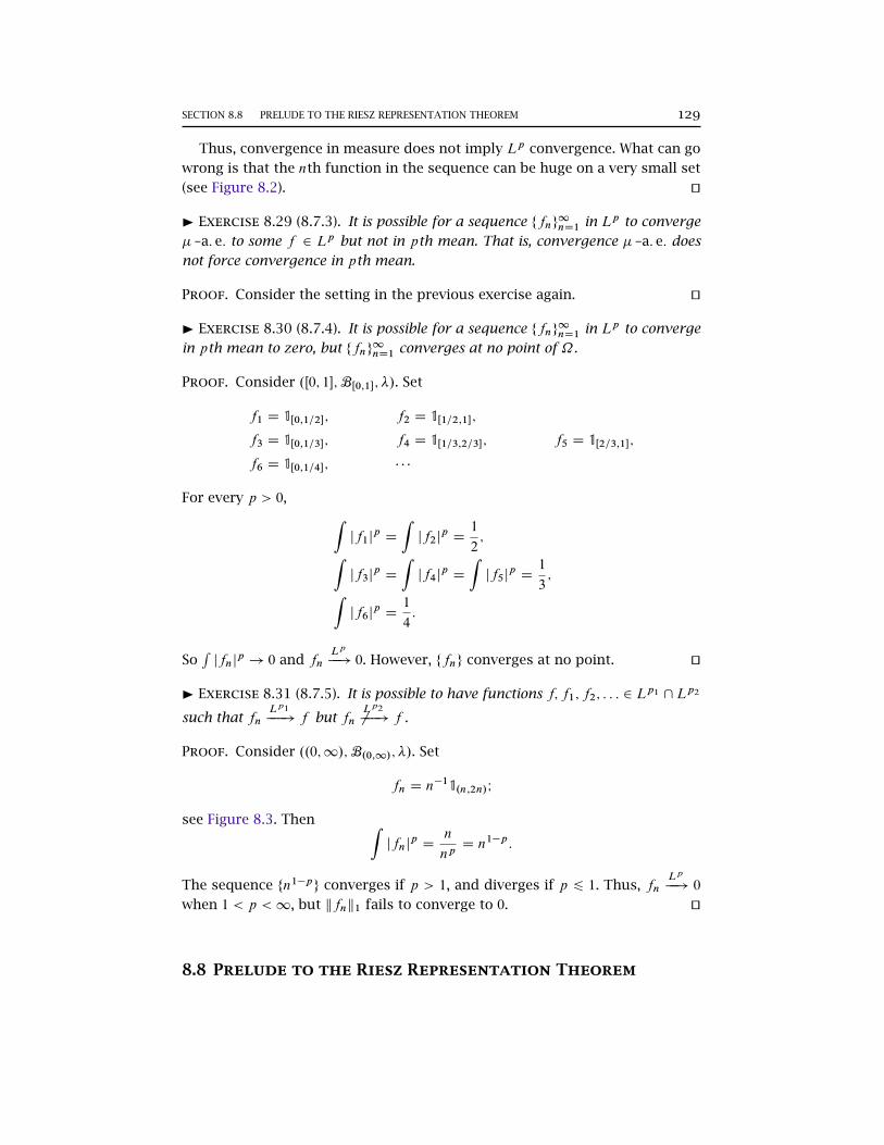
SECTION 8.8 PRELUDE TO THE RIESZ REPRESENTATION THEOREM 129
Thus, convergence in measure does not imply Lp convergence. What can go
wrong is that the nth function in the sequence can be huge on a very small set
(see Figure 8.2). ut
I Exercise 8.29 (8.7.3). It is possible for a sequence ffng1nD1 in Lp to converge
� –a: e: to some f 2 Lp but not in pth mean. That is, convergence � –a: e: does
not force convergence in pth mean.
Proof. Consider the setting in the previous exercise again. ut
I Exercise 8.30 (8.7.4). It is possible for a sequence ffng1nD1 in Lp to converge
in pth mean to zero, but ffng1nD1 converges at no point of ˝.
Proof. Consider .Œ0; 1�;BŒ0;1�; �/. Set
f1 D 1Œ0;1=2�; f2 D 1Œ1=2;1�;
f3 D 1Œ0;1=3�; f4 D 1Œ1=3;2=3�; f5 D 1Œ2=3;1�;
f6 D 1Œ0;1=4�; � � �
For every p > 0, Zjf1j
pD
Zjf2j
pD1
2;Z
jf3jpD
Zjf4j
pD
Zjf5j
pD1
3;Z
jf6jpD1
4:
SoRjfnj
p ! 0 and fnLp
��! 0. However, ffng converges at no point. ut
I Exercise 8.31 (8.7.5). It is possible to have functions f; f1; f2; : : : 2 Lp1 \Lp2
such that fnLp1���! f but fn 6
Lp2���! f .
Proof. Consider ..0;1/;B.0;1/; �/. Set
fn D n�11.n;2n/I
see Figure 8.3. Then Zjfnj
pD
n
npD n1�p:
The sequence fn1�pg converges if p > 1, and diverges if p 6 1. Thus, fnLp
��! 0
when 1 < p <1, but kfnk1 fails to converge to 0. ut
8.8 Prelude to the Riesz Representation Theorem
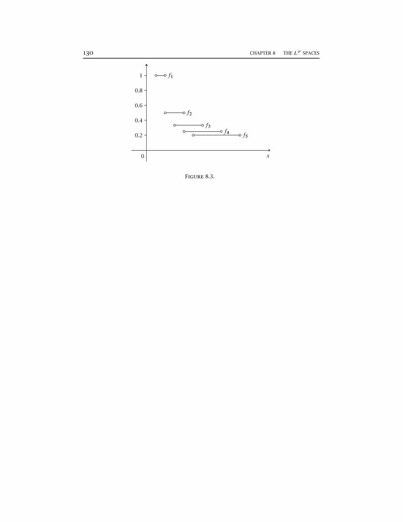
130 CHAPTER 8 THE LP SPACES
0 x
0.2
0.4
0.6
0.8
1 f1
f2
f3f4
f5
Figure 8.3.
9THE RADON-NIKODYM THEOREM
9.1 The Radon-Nikodym Theorem, Part I
I Exercise 9.1 (9.1.1). In the definition of an additive set function, show that
the seriesP1nD1 '.An/ must converge absolutely.
Proof. Observe thatS1nD1An D
S1kD1Ank for every rearrangement fnkg1kD1
of the positive integers, hence bothP1nD1 '.An/ and
P1kD1 '.Ank / should be
defined and equal, that is, the series is unconditionally convergent. By the
Riemann series theorem, it is absolutely convergent. ut
I Exercise 9.2 (9.1.2). In Claim 4, quickly verify that '� is a finite measure
with support A�.
Proof. For all A 2 F we have A \ A� � A�, and the negativity of A� with
respect to ' implies that '�.A/ D �'.A \ A�/ > 0. Therefore, '� is nonnega-
tive. Next, '�.¿/ D '.¿/ D 0. We now exhibit countable additivity for '�. Let
fAng1nD1 denote a disjoint sequence of F -sets. Then
'�
0@ 1[nD1
An
1A D �'0B@0@ 1[nD1
An
1A \ A�1CA D �'
0@ 1[nD1
.An \ A�/
1AD �
1XnD1
' .An \ A�/
D
1XnD1
��' .An \ A
�/�
D
1XnD1
'�.An/:
This shows that '� is a measure. Since '� .˝/ D �' .A�/ 2 R, '� is a fi-
nite measure. To see that A� is a support of '�, observe that '��.A�/c
�D
�'�.A�/c \ A�
�D �'.¿/ D 0. ut
131
132 CHAPTER 9 THE RADON-NIKODYM THEOREM
I Exercise 9.3 (9.1.3). Suppose that�AC; A�
�and
�BC; B�
�are Hahn de-
compositions with respect to an additive set function '. Then '�AC�BC
�D
' .A��B�/ D 0.
Proof. We first do the set operations:
AC�BC D .AC [ BC/ X .AC \ BC/ D .AC [ BC/ X�A�c \ B�c
�D .AC [ BC/ X .A� [ B�/c
D .AC [ BC/ \ .A� [ B�/
D
�AC \ B�
�[
�A� \ BC
�;
and�AC \ B�
�\�A� \ BC
�D ¿. Since AC \ B� � AC, we have '
�AC \ B�
�>
0; since AC \ B� � AC � B�, we have '�AC \ B� � AC
�6 0; hence,
'�AC \ B� � AC
�D 0. Similarly, '
�A� \ BC
�D 0, and so '
�AC�BC
�D 0.
Using this way, we can also show that ' .A��B�/ D 0. ut
I Exercise 9.4 (9.1.4). The Jordan decomposition of an additive set function '
is unique.
Proof. Let�AC; A�
�and
�BC; B�
�denote Hahn decomposition of ˝ with re-
spect to '. Let 'CA .E/ D '�E \ AC
�and 'CB .E/ D '
�E \ BC
�for every E 2 F ;
define '�A and '�B similarly. Then ' D 'CA �'�A is the Jordan decomposition of '
relative to the Hahn decomposition�AC; A�
�and ' D 'CB �'
�B is the Jordan de-
composition of ' relative to the Hahn decomposition�BC; B�
�. We now show
that 'CA D 'C
B and '�A D '�B . For any E 2 F , we have
'CA .E/ D '�E \ AC
�D '
�E \
�BC [ B�
�\ AC
�D '
�E \ AC \ BC
�C '
�E \ AC \ B�
�D '
�E \ AC \ BC
�;
where '�E \ AC \ B�
�D 0 since: (i) E\AC\B� � AC implies that '.E\AC\
B�/ > 0; (ii) E \AC \B� � B� implies that '�E \ AC \ B�
�6 0. Similarly, we
can show 'CB D '�E \ AC \ BC
�D 'CA and '�A D '
�B . ut
I Exercise 9.5 (9.1.5). This problem relates somewhat the notion of absolute
continuity with the familiar "-ı concepts.
a. Let � and � denote measures with common domain F and such that � is
finite. Then � � � iff for every " > 0 there is ı > 0 such that �.A/ < ı forces
�.A/ < ".
b. The claim in (a) is not necessarily true if � is infinite, since the condition � � �
does not imply the "-ı condition.
SECTION 9.1 THE RADON-NIKODYM THEOREM, PART I 133
Proof. (a) Suppose first that for every " > 0 there is ı > 0 such that �.A/ < ı
forces �.A/ < ". We desire to show that � � �. If �.A/ D 0 and " > 0 is given
(and the corresponding ı is found), then �.A/ < ı, hence �.A/ < ". Since " > 0
is arbitrary, it follows that �.A/ D 0, whence � � �.
To show the other direction, suppose that there is " > 0 such that for every
ı > 0 there is a set A 2 F with �.A/ < ı and �.A/ > ". In particular, there is
" > 0 such that there is a sequence fAng1nD1 of F -sets with �.A/ < 1=n2 and
�.A/ > " for each n 2 N. Let A D limAn DT1nD1
S1mDnAm. For every n 2 N we
have
�.A/ 6 �
0@ 1[mDn
Am
1A 6 1XmDn
� .Am/ <
1XmDn
1
m2;
so �.A/ D 0. However, we also have
�.A/ D ��limAn
�> lim �.An/ > " > 0
by property (M10) in Section 2.2. This shows that there is A 2 F such that
�.A/ D 0 and �.A/ > 0, so � 6� �.
(b) Let ˝ D Z, let F D 2˝ , let � denote the counting measure, so that �
is infinite, and let � be such that ��fng�D
1n2
for each n 2 Z, so that � is
finite. ut
I Exercise 9.6 (9.1.6). Let �, �, �1, and �2 denote measures, each having com-
mon domain F .
a. If �1 ? � and �2 ? �, then �1 C �2 ? �.
b. If �1 � � and �2 � �, then �1 C �2 � �.
c. If �1 � � and �2 ? �, then �1 ? �2.
d. If � � � and � ? �, then � D 0.
e. If � ? �, then � D 0.
f. If � and � are � -finite with � � �, then �.f! 2 ˝ W d�d� .!/ D 0g/ D 0.
Proof. (a) Let �1 ? � and �2 ? �. Then there exist D1 2 F with �1 .D1/ D
��Dc1
�D 0, and D2 2 F with �2 .D2/ D �
�Dc2
�D 0. Let D D D1 \D2. We show
that D supports � and Dc supports �1 C �2. As for �, we have
��Dc�D �
�Dc1 [D
c2
�6 �
�Dc1
�C �
�Dc2
�D 0:
As for �1 C �2, we have
.�1 C �2/ .D/ D �1 .D1 \D2/C �2 .D1 \D2/ 6 �1 .D1/C �2 .D2/ D 0:
Therefore, .�1 C �2/ .D/ D � .Dc/ D 0, that is, �1 C �2 ? �.
(b) If �.A/ D 0, then .�1 C �2/.A/ D �1.A/C �2.A/ D 0; hence, �1 C �2 � �.
134 CHAPTER 9 THE RADON-NIKODYM THEOREM
(c) Since �2 ? �, there exists D 2 F with �2 .D/ D � .Dc/ D 0; since �1 �
�, � .Dc/ D 0 forces �1 .Dc/ D 0. Therefore, there is D 2 F with �1 .Dc/ D
�2 .D/ D 0, that is, �1 ? �2.
(d) Since � ? �, there is D 2 F with � .D/ D � .Dc/ D 0. For any E 2 F , we
have
�.E/ D � .E \D/C ��E \Dc
�D 0C 0 D 0;
where � .E \D/ D 0 since � .E \D/ 6 � .D/ D 0, and � .E \Dc/ 6 � .Dc/ D 0
since � .Dc/ D 0 and � � �.
(e) Let � D � in (d) and we get the result.
(f) We have
�Œd�=d� D 0� D
ZŒd�=d�D0�
d�
d�d� D 0: ut
I Exercise 9.7 (9.1.8). Let f 2 L1.˝;F ; �/. Define �.E/ DREf d� for every
E 2 F .
a. � is an additive set function such that �C.E/ DREf C d� and ��.E/ DR
Ef � d� for every E 2 F .
b. If AC D f! 2 ˝ W f .!/ > 0g and A� D ACc , then .AC; A�/ is a Hahn decom-
position with respect to �.
Proof. (b) We first show (b). For every E 2 F with E � AC, we have
�.E/ D
ZE
f d� D
ZE\AC
f d� D
ZE
f 1AC d� D
ZE
f C d� > 0;
and for every E 2 F with E � A� we have
�.E/ D
ZE
f d� D
ZE\A�
f d� D
ZE
f 1A� d� D
ZE
f � d� 6 0:
Hence, .AC; A�/ is a Hahn decomposition with respect to �.
(a) It follows from (L6) (p. 251) that � is an additive set function. Now by part
(b) and the uniqueness of Hahn decomposition (Exercise 9.3), we get the de-
sired result. ut
I Exercise 9.8 (9.1.9). Let M denote the collection of additive set functions '
with domain F .
a. M is a linear space over R: for a; b 2 R and '1; '2 2M we have a'1Cb'2 2M.
b. Given ' 2M, define k'k D 'C.˝/C '�.˝/, where ' D 'C � '� is the Jordan
decomposition of '. Then k k is a norm on M.
c. Is M a Banach space?
SECTION 9.1 THE RADON-NIKODYM THEOREM, PART I 135
Proof. (a) It is clear that a'1 C b'2 W F ! R, and for a disjoint sequence
fAng � F we have
.a'1 C b'2/
0@ 1[nD1
An
1A D a'10@ 1[nD1
An
1AC b'20@ 1[nD1
An
1AD
1XnD1
a'1.An/C
1XnD1
b'2.An/
D
1XnD1
�a'.An/C b'2.An/
�D
1XnD1
.a'1 C b'2/.An/:
(b) Clearly, k'k > 0 for all ' 2M, and kok D 0, where o.E/ D 0 for all E 2 F .
Now if k'k D 0, then 'C.˝/ C '�.˝/ D 0 implies that 'C.˝/ D '�.˝/ D 0.
Since 'C and '� are finite measures on F (by Claim 4, p. 373), for every E 2 F
we have 'C.E/ 6 'C.˝/ D 0 and '�.E/ 6 '�.˝/ D 0; that is,
'.E/ D 'C.E/ � '�.E/ D 0:
We finally show that the triangle inequality. Let '1; '2 2M. Then
k'1 C '2k D .'1 C '2/C.˝/C .'1 C '2/
�.˝/
6 'C1 .˝/C 'C2 .˝/C '
�1 .˝/C '
�.˝/
D k'1k C k'2k:
This proves that .M; k k/ is a normed space. ut
I Exercise 9.9 (9.1.10). Let .AC; A�/ denote a Hahn decomposition of the ad-
ditive set function ', and let ' D 'C � '� denote the Jordan decomposition. We
have
'C.A/ D supf'.E/ W E 2 F ; E � Ag;
'�.A/ D � inff'.E/ W E 2 F ; E � Ag;
for every A 2 F .
Proof. Let A;E 2 F with E � A. Then
'.E/ D '.E \ AC/C '.E \ A�/ D 'C.E/ � '�.E/ 6 'C.E/ 6 'C.A/:
Thus, 'C.A/ is an upper bound of f'.E/ W E 2 F ; E � Ag. We next show that
'C.A/ is actually in the former set: let E D A \ AC. Then E 2 F , E � A, and
'.E/ D '.A \ AC/ D 'C.A/:
We then have
136 CHAPTER 9 THE RADON-NIKODYM THEOREM
'�.A/ D 'C.A/ � '.A/ D supf'.E/ W E 2 F ; E � Ag � '.A/
D supf'.E/ � '.A/ W E 2 F ; E � Ag
D supf�'.A XE/ W E 2 F ; E � Ag
D supf�'.F / W F 2 F ; F � Ag
D � inff'.F / W F 2 F ; F � Ag: ut
I Exercise 9.10 (9.1.12). Let �, �, �1, �2 and � denote � -finite measures having
domain F . We have the following claims.
a. If �1 � � and �2 � �, then d .�1 ˙ �2/ =d� D d�1=d�˙d�2=d� � –a: s: on ˝.
b. If � � � and �� �, then � � � and d�d� D
d�d�
d�d� � –a: e: on ˝.
c. If � � � and �� �, then d�d� D 1Œd�=d�>0� �
1d�=d� � –a: e: on ˝.
d. Let � � � and � � �. Then � � � if and only if �Œd�d� > 0; d�d� > 0� D 0, in
which case we have
d�
d�D 1Œd�=d�>0� �
d�=d�
d�=d�� –a: s: on ˝:
Proof. (a) Since �1 � � and �2 � �, we get �1 ˙ �2 � �, and that for every
E 2 F ,
�1.E/ D
ZE
d�1d�
d�; �2.E/ D
ZE
d�2d�
d�;
and
.�1 ˙ �2/.E/ D
ZE
d.�1 ˙ �2/
d�d�:
Clearly, .�1 ˙ �2/.E/ D �1.E/˙ �2.E/. Hence,
d.�1 ˙ �2/
d�D
d�1d�˙
d�2d�
:
(b) Let � � � and � � �. Take an arbitrary E 2 F so that �.E/ D 0; then
�.E/ D 0; then �.E/ D 0 and so � � �. Next, for every E 2 F , we have
�.E/ D
ZE
d�
d�d�; �.E/ D
ZE
d�
d�d�; and �.E/ D
ZE
d�
d�d�:
It follows from (L14) (p. 259) that
�.E/ D
ZE
d�
d�d� D
ZE
d�
d�
d�
d�d�I
that is, d�d� D
d�d�
d�d� .
(c) It follows from (b) thatd�
d�D
d�
d�
d�
d�:
Therefore,
SECTION 9.1 THE RADON-NIKODYM THEOREM, PART I 137
d�
d�D 1Œd�=d�>0� �
1
d�=d�:
(d) ut
I Exercise 9.11 (9.1.15). Suppose that � and � are � -finite measures on F . The
Lebesgue decomposition of � with respect to � is unique. That is, if � D �ac C �s
where �ac and �s are � -finite measures with �ac � � and �s ? �, and if in
addition � D �0ac C �0s where �0ac and �0s are � -finite measures with �0ac � � and
�0s ? �, then �ac D �0ac and �s D �
0s.
Proof. Since �s ? �, there exists A 2 F such that A supports �s and Ac
supports �; that is,
�s.Ac/ D �.A/ D 0:
Since �0s ? �, there exists B 2 F such that B supports �0s and Bc supports �;
that is,
�0s.Bc/ D �.B/ D 0:
Since �s.Ac \ Bc/ 6 �s.A
c/ D 0, and �0s.Ac \ Bc/ 6 �0s.B
c/ D 0, we have that
A[B supports both �s and �0s. Since �.A[B/ 6 �.A/C�.B/ D 0, we have that
.A [ B/c supports �. Let S ´ A [ B , so that
�.S/ D �s.Sc/ D �0s.S
c/ D 0
We now show that �ac D �0ac. For every E 2 F , we have
�ac.E/ D �ac.E \ Sc/C �ac.E \ S/ D �ac.E \ S
c/ Œ�ac � ��
D �ac.E \ Sc/C �s.E \ S
c/
D �.E \ Sc/
D �0ac.E \ Sc/C �0s.E \ S
c/
D �0ac.E \ Sc/
D �0ac.E \ Sc/C �0ac.E \ S/
D �0ac.E/:
Hence, �ac D �0ac, and so �s D �
0s. ut

10PRODUCTS OF TWO MEASURE SPACES
10.1 Product Measures
Remark 10.1.
.A \ B/ � .C \D/ D .A � C/ \ .B �D/ ;
.A [ B/ � .C [D/ ¤ .A � C/ [ .B �D/ ;
A � .B \ C/ D .A � B/ \ .A � C/ ;
A � .B [ C/ D .A � B/ [ .A � C/ :
I Exercise 10.2 (10.1.1). Let ˝1 denote an uncountable set, and let F1 denote
the � -field of subsets of ˝1 that are at most countable or have at most countable
complements. Let ˝2 and F2 be identical to ˝1 and F1, respectively. Let D D
f.!1; !2/ 2 ˝1 � ˝2 W !1 D !2g. We have D!1 2 F2 and D!2 2 F1 for every
!1 2 ˝1 and !2 2 ˝2, but D … F1 ˝ F2.
Proof. For every !1, we have D!1 D f!2g with !2 D !1. For every !2 2 ˝2, we
have D!2 D f!1g with !1 D !2. Hence, D!1 2 F2 and D!2 2 F1. ut
I Exercise 10.3 (10.1.2). Let A � ˝1 and B � ˝2.
a. Suppose that A � B ¤ ¿. Then A � B 2 F1 ˝ F2 iff A 2 F1 and B 2 F2.
b. Suppose that A�B D ¿. Then obviously A�B 2 F1˝F2, but it is not always
the case that A 2 F1 and B 2 F2.
Proof. (a) The if part is evident since F1�F2 � F1˝F2. Now take an arbitrary
!1 2 A (such a point exists because A � B ¤ ¿ implies that A ¤ ¿). Then
.A � B/!1 D B 2 F2. Similarly we show that A 2 F1.
(b) If there exists A … F1, then we have A � ¿ D ¿ 2 F1 ˝ F2. But obviously
A … F1. ut
I Exercise 10.4 (10.1.3). Prove the following set-theoretical facts.
139
140 CHAPTER 10 PRODUCTS OF TWO MEASURE SPACES
a. Let A1�B1 and A2�B2 both be nonempty. Then A1�B1 � A2�B2 iff A1 � A2and B1 � B2.
b. Let A1�B1 and A2�B2 both be nonempty. Then A1�B1 D A2�B2 iff A1 D A2and B1 D B2.
c. Let A�B , A1�B1, and A2�B2 be nonempty. Then A�B is the disjoint union
of A1 � B1 and A2 � B2 iff either (i) A is the disjoint union of A1 and A2 and
B D B1 D B2 or (ii) A D A1 D A2 and B is the disjoint union of B1 and B2.
d. The “only if” parts of (a) and (b) do not necessarily hold for empty Cartesian
products. What about (c)?
Proof. (a) The if part is automatic, so we only do the only if part. Suppose
that A1 � B1 � A2 � B2. If, say, A1 6� A2, then there exists !01 2 A1 X A2.
Take an arbitrary !2 2 B1. Then .!01; !2/ 2 A1 � B1 but .!01; !2/ … A2 � B2. A
contradiction.
(b) Using the fact that A1 � B1 D A2 � B2 iff A1 � B1 � A2 � B2 and A2 � B2 �
A1 � B1, and the result in (a), we get the desired outcome.
(c) Straightforward. ut
I Exercise 10.5 (10.1.5). Let F1 and F2 denote � -fields on ˝1 and ˝2, respec-
tively. It may not be the case that F1 � F2 is a � -field on ˝1 �˝2.
Proof. Consider .Rk ;Bk ; �k/ and .Rm;Bm; �m/. Then Bk �Bm � Bk ˝Bm. ut
I Exercise 10.6 (10.1.6). Prove Claims 2(b) and 3(b) by mimicking the proofs
of Claims 2(a) and 3(a).
Proof. (2(b)) We show that if E 2 F1 ˝ F2, then E!2 2 F1 for every !2 2 ˝2.
Define
D D fE 2 F1 ˝ F2 W E!2 2 F1 for every !2 2 ˝2g:
First observe that ˝1 � ˝2 2 F1 � F2 � F1 ˝ F2 and .˝1 � ˝2/!2 D ˝1 2 F1
for every !2 2 ˝2. Therefore, ˝1 � ˝2 2 D . Next, if E 2 D , then we have
Ec 2 F1 ˝ F2 and .Ec/!2 D .E!2/c 2 F1 for every !2 2 ˝2, so that Ec 2 D .
Next, if fEng is a sequence of D-sets, thenSEn 2 F1 ˝ F2 and .
SEn/
!2 DS.En/
!2 2 F1 for every !2 2 ˝2, whenceSEn 2 D . Therefore, D is a � -field
on ˝1 � ˝2 and D � F1 ˝ F2. We desire to strengthen this inclusion to an
equality. To do this, let E1 2 F1 and E2 2 F2. Then for every !2 2 ˝2 we have
.E1 �E2/!2 D
˚E1 if !2 2 E2
¿ if !2 … E22 F1:
This shows that F1 � F2 � D . Since D is a � -filed, we have F1 ˝ F2 � D . This
yields D D F1 ˝ F2.
SECTION 10.1 PRODUCT MEASURES 141
(3(b)) We show that if f W ˝1 � ˝2 ! xR be F1 ˝ F2=B�-measurable, then f !2
is F1=B�-measurable for every !2 2 ˝2. To do this, first consider the case of
f D 1E , where E 2 F1 ˝ F2. Next, pick !1 2 ˝1 and !2 2 ˝2. We have
.1E /!2.!1/ D 1 () 1E .!1; !2/ D 1 () .!1; !2/ 2 E () !1 2 E
!2
() 1E!2 .!1/ D 1;
and hence
.1E /!2 D 1E!2 :
By Claim 2(b), E 2 F1 ˝ F2 forces E!2 2 F1. Therefore, if f D 1E where
E 2 F1 ˝ F2, we have that f !2 is the indicator function 1E!2 of the F1-set
E!2 , and hence is F1=B�-measurable. This proves 3(b) when f is an indicator
function on ˝1 �˝2 of a set in F1 ˝ F2.
Next, let f DPniD1 ci1Ei , where E1; : : : ; En 2 F1˝F2 are disjoint with union
˝1 � ˝2 and c1; : : : ; cn 2 R, so that f is an F1 ˝ F2=B�-measurable simple
function on ˝1 � ˝2. For every !2 2 ˝2, observe that f !2 DPniD1 ci1.Ei /!2 ,
a finite linear combination of the indicator functions .1E1/!2 ; : : : ; .1En/
!2 , and
each of these is F1=B�-measurable by the previous paragraph. It follows that
f !2 is F1=B�-measurable for every !2 2 ˝2. This proves the result when f is
an F1 ˝ F2=B�-measurable simple function on ˝1 �˝2.
Next, suppose that f is a nonnegative F1 ˝ F2=B�-measurable function on
˝1 � ˝2. There exists a nondecreasing sequence fsng of nonnegative finite-
valued F1 ˝ F2=B�-measurable simple functions on ˝1 �˝2 with limn sn D f .
By the previous paragraph, we have that .sn/!2 is F1=B�-measurable for every
!2 2 ˝2 and n 2 N. Since
f !2 D
�limnsn
�!2D lim
n.sn/
!2
for every !2 2 ˝2, we have that f !2 is the limit of a sequence of F1=B�-
measurable functions and hence is itself F1=B�-measurable. This proves the
result when f is a nonnegative F1 ˝ F2=B�-measurable function on ˝1 �˝2.
Finally, if f is a general F1 ˝ F2=B�-measurable function on ˝1 �˝2, then
the functions f C and f �, both being nonnegative F1 ˝ F2=B�-measurable
functions on ˝1 �˝2, are such that .f C/!2 and .f �/!2 are F1=B�-measurable
for every !2 2 ˝2. Observing that
f !2 D .f C � f �/!2 D .f C/!2 � .f �/!2
for every !2 2 ˝2, we see for every !2 2 ˝2 that f !2 is the difference of two
F1=B�-measurable functions on ˝1�˝2 and hence is F1=B
�-measurable. This
completes the proof. ut
I Exercise 10.7 (10.1.7). The product of .Rk ;Bk ; �k/ and .Rm;Bm; �m/ is
.RkCm;BkCm; �kCm/:
142 CHAPTER 10 PRODUCTS OF TWO MEASURE SPACES
In other words, Bk ˝Bm D BkCm and �k ˝ �m D �kCm.
Proof. We first show that Bk ˝ Bm D BkCm visa showing that Bk � Bm �
BkCm (proper subset). Consider the projection �k W RkCm ! Rk . Let Ok and
OkCm be the set of open sets of Rk and RkCm, respectively. Endowed with
Tychonoff’ topology, �k is continuous. Hence,
��1k .Bk/ D ��1k .�.Ok// D �.��1k .Ok// � �.OkCm/ D BkCm:
Similarly, we have ��1m .Bm/ � BkCm. Therefore,
Bk�Bm
D ��1k .Bk/ \ ��1m .Bm/ � BkCm:
To see that the containment is strict, observe that the open unit ballD in BkCm
cannot be written as A1�A2 with A1 � Rk and A2 � Rm, let along with A1 2 Bk
and A2 2 Bm. From the above argument, we have
Bk˝Bm
D �.Bk�Bm/ � BkCm:
Define A1 D intervals of the form .�1; x�. We have AkCm1 D Ak
1 �Am1 � Bk �
Bm; hence,
BkCmD �.AkCm
1 / � �.Bk�Bm/ D Bk
˝Bm:
It follows from Claim 4 of Section 4.2 that �kCm.A � B/ D �k.A/�m.B/ for
every A 2 Bk and B 2 Bm. Since .Rk ;Bk ; �k/ and .Rm;Bm; �m/ are � -finite, by
Claim 6 we have �kCm D �k ˝ �m. ut
I Exercise 10.8 (10.1.8). Let ˝1 D ˝2 D Œ0; 1�. Let F1 D F2 denote the Borel
subsets of Œ0; 1�. Let �1 denote Lebesgue measure restricted to F1, and let �2denote the counting measure on Œ0; 1�. Let E D f.!1; !2/ 2 ˝1 �˝2 W !1 D !2g.
a. E 2 F1 ˝ F2.
b.R˝1�2.E!1/d�1.!1/ D 1.
c.R˝2�1.E
!2/d�2.!2/ D 0.
Proof. (a) We prove E 2 F1˝F2 by showing that E is closed in Œ0; 1�� Œ0; 1�. It
is true because Œ0; 1� is Hausdorff (see Willard, 2004, Theorem 13.7).
(b) Since �2 is a counting measure, we haveZ˝1
�2.E!1/d�1.!1/ D
Z˝1
�2.!2/d�1.!1/ D
Z˝1
1d�1.!1/ D 1:
(c) We haveZ˝2
�1.E!2/d�2.!2/ D
Z˝2
�1.!1/d�2.!2/ D
Z˝2
0d�2.!2/ D 0: ut
I Exercise 10.9 (10.1.10, Cavalieri’s Principle). If E;F 2 F1˝F2 are such that
�2.E!1/ D �2.F!1/ for every !1 2 ˝1, then �1 ˝ �2.E/ D �1 ˝ �2.F /.
SECTION 10.2 THE FUBINI THEOREMS 143
Proof. We have
�1 ˝ �2.E/ D
Z˝1
�2.E!1/d�1 D
Z˝1
�2.F!1/d�1 D �1 ˝ �2.F /: ut
10.2 The Fubini Theorems

11ARBITRARY PRODUCTS OF MEASURE SPACES
11.1 Notation and Conventions
I Exercise 11.1 (11.1.1). Let ˝1 denote a nonempty set, and let A denote a
nonempty collection of subsets of ˝1. Let ˝2 denote a nonempty set, and let B
denote a nonempty collection of subsets of ˝2.
a. Let B � ˝2 be nonempty. Then �˝1�B.A � fBg/ D �.A/ � fBg.
b. �.A �B/ D �.�.A/ � �.B//.
Proof. (a) Since A � fBg � �.A/ � fBg, and �.A/ � fBg is a � -field on ˝1 � B ,
we get
�˝1�B.A � fBg/ � �.A/ � fBg:
To see the converse inclusion, define
C ´˚A 2 �.A/ W A � B 2 �˝�B.A � fBg/
:
If A 2 A, then A � B 2 A � fBg � �˝1�B.A � fBg/, so A 2 C ; thus A � C . We
then show that C is a � -field. (i) ˝1 2 C . (ii) If A 2 C , then .A � B/c D Ac � B 2
�˝1�B.A � fBg/, i.e., Ac 2 C . (iii) If fAng1nD1 � C , then .SAn/ � B D
S.An � B/,
i.e.,SAn 2 C . Therefore, �.A/ D C .
(b) Since A �B � �.A/ � �.B/, we have
�.A �B/ � �.�.A/ � �.B//:
Next, for every B 2 �.B/ we have �.A/ � fBg D �˝1�B.A � fBg/ � �.A �B/ by
(a). Therefore, [B2�.B/
��.A/ � fBg
�� �.A �B/I
that is, �.A/ � �.B/ � �.A �B/. But then �.�.A/ � �.B// � �.A �B/. ut
I Exercise 11.2 (11.1.2). Prove the claim in the Identification Lemma for the
case where P is a two-element set, which case is really the only one that we use.
145
146 CHAPTER 11 ARBITRARY PRODUCTS OF MEASURE SPACES
Proof. By the assumption, P D f1; 2g. Then
N0 D FD1 � FD2 :
Let A1 denote the collection of sets of the form�i2D1Ai , where Ai 2 Fi for
each i 2 D1 and at most finitely many Ai ’s differ from ˝i . Then FD1 D �.A1/.
Let A2 denote the collection of sets of the form�i2D2Ai , where Ai 2 Fi for
each i 2 D2 and at most finitely many Ai ’s differ from ˝i . Then FD2 D �.A2/,
and
N1 D A1 �A2:
Therefore, �.N0/ D �.N1/ iff
�.�.A1/ � �.A2// D �.A1 �A2/:
The above equality follows from Exercise 11.1(b) immediately. ut
I Exercise 11.3 (11.1.3). Prove the Identification Lemma in full generality for
the case where P is an arbitrary set.
Proof. By definition, N0 is the collection of sets�p2P ADp , where ADp 2 FDpfor each p 2 P and ADp ¤ ˝Dp for at most finitely many p 2 P . Further, N1 is
the collection of sets of the form
�p2P
�i2Dp
Ai
!;
where Ai ¤ ˝i for at most finitely many i 2Sp2P Dp . For each p 2 P , let ADp
denote the collection of�i2DpAi . We then have
�.N0/ D �
�p2P
FDp
!;
�.N1/ D �
�p2P
ADp
!:
Notice that FDp D �.ADp / for every p 2 P . Thus we need to show that
�
�p2P
�.ADp /
!D �
�p2P
ADp
!:
Generalizing the result in Exercise 11.1(b) yields the desired outcome. ut
I Exercise 11.4 (11.1.4). Show that EF is a semiring on ˝F .
Proof. Given a finite subset F � I , we define EF by writing
EF D
(�i2F
Ai W Ai 2 Fi for every i 2 F
):
SECTION 11.2 CONSTRUCTION OF THE PRODUCT MEASURE 147
Clearly, ¿ 2 EF . Take two sets B;C 2 EF and write them as B D�i2F Bi and
C D�i2F Ci , where Bi ; Ci 2 Fi for each i 2 F . Then
B \ C D
�i2F
Bi
!\
�i2F
Ci
!D�i2F
.Bi \ Ci / 2 EF :
Finally, suppose that ¿ ¤ B � C (otherwise the proof is trivial). Then Bi � Cifor every i 2 F . It is easy to see that C X B is a finite disjoint union of EF -
sets. ut
I Exercise 11.5 (11.1.5). Let A denote a semiring on ˝1, and let B denote a
semiring on ˝2. Then A �B is a semiring on ˝1 �˝2.
Proof. It is evident that A�B contains ¿ and is a �-system. Now let A1�B1 �
A2 � B2, where A1; A2 2 A and B1; B2 2 B. Then A1 � A2 and B1 � B2, and
.A2 � B2/ X .A1 � B1/ D ŒA1 � .B2 X B1/� t Œ.A2 X A1/ � B2�:
Observe that B2 X B1 may be written as a finite disjoint unionFkiD1Di of B-
sets, and A2 X A1 may be written as a finite disjoint unionF`jD1 Cj . It follows
that
.A2 � B2/ X .A1 � B1/ D
264A1 �0@ kGiD1
Di
1A375 t
2640@G̀jD1
Cj
1A � B2375
D
24 kGiD1
.A1 �Di /
35 t24G̀jD1
.Cj � B2/
35 :Hence .A2 � B2/ X .A1 � B1/ is a finite disjoint union of sets in A �B. ut
11.2 Construction of the Product Measure
I Exercise 11.6 (11.2.1). Refer to the proof of Claim 4.
a. Prove Subclaim 1.
b. Prove Subclaim 2.
c. Why can’t we use the same type of proof as used to demonstrate the finite
additivity of � to show that � as defined on H is countably additive?
Proof. (a) We show that if AF1 2 FF1 , then there exists CF1[F2 2 FF1[F2 with
the property that
˚�1F1 .AF1 �˝Fc1/ D ˚�1F1[F2.CF1[F2 �˝.F1[F2/c /: (11.1)
Define the collection
148 CHAPTER 11 ARBITRARY PRODUCTS OF MEASURE SPACES
C ´˚AF1 2 FF1 W there is CF1[F2 2 FF1[F2 such that (11.1) holds
:
Then C � FF1 .
We first show that EF1 � C . Take an arbitrary�i2F1Ai 2 EF1 . Then
˚�1F1
24 �i2F1
Ai
!�˝F c
1
35 D�i2I
Qi ;
where Qi D Ai for each i 2 F1 and Qi D ˝i for each i 2 F c1 . Define the set
CF1[F2 D �i2F1[F2
Ri ;
where Ri D Ai for each i 2 F1 and Ri D ˝i for each i 2 F2. We have CF1[F2 2
EF1[F2 � FF1[F2 , and
˚�1F1[F2
�CF1[F2 �˝.F1[F2/c
�D�
i2I
Qi :
Comparing the last two displayed equations shows that�i2F1Ai 2 C . That is,
we have EF1 � C .
We now turn to showing that C is a � -filed on ˝F1 . We first show that ˝F1 2
C . This is because
˚�1F1 .˝F1 �˝Fc1/ D ˝ D ˚�1F1[F2.˝F1[F2 �˝.F1[F2/c /;
and ˝F1[F2 2 FF1[F2 . We now discuss closure under complementation. Sup-
pose that AF1 2 C , and let CF1[F2 2 FF1[F2 be such that (11.1) holds. Then
˚�1F1 .AcF1�˝F c
1/ D ˚�1F1
h.˝F1 �˝F c1 / X .AF1 �˝F
c1/i
D ˚�1F1 .˝F1 �˝Fc1/ X ˚�1F1 .AF1 �˝F
c1/
D ˚�1F1[F2
�˝F1[F2 �˝.F1[F2/c
�X ˚�1F1[F2
�CF1[F2 �˝.F1[F2/c
�D ˚�1F1[F2
h�˝F1[F2 �˝.F1[F2/c
�X�CF1[F2 �˝.F1[F2/c
�iD ˚�1F1[F2
�C cF1[F2 �˝.F1[F2/c
�:
Since C cF1[F2 2 FF1[F2 , it follows that AcF1 2 C .
We now show that C is closed under countable intersections. Let fA.n/F1 g � C ,
and let C .n/F1[F22 FF1[F2 denote the corresponding sets for A.n/F1 that satisfies
(11.1) for every n 2 N:
˚�1F1
�A.n/F1�˝F c
1
�D ˚�1F1[F2
�C.n/F1[F2
�˝.F1[F2/c�:
We have
SECTION 11.2 CONSTRUCTION OF THE PRODUCT MEASURE 149
˚�1F1
2640@ 1\nD1
A.n/F1
1A �˝F c1
375 D ˚�1F124 1\nD1
�A.n/F1�˝F c
1
�35D
1\nD1
˚�1F1
�A.n/F1�˝F c
1
�D
1\nD1
˚�1F1[F2
�C.n/F1[F2
�˝.F1[F2/c�
D ˚�1F1[F2
24 1\nD1
�C.n/F1[F2
�˝.F1[F2/c�35
D ˚�1F1[F2
2640@ 1\nD1
C.n/F1[F2
1A �˝.F1[F2/c375 :
SinceT1nD1 C
.n/F1[F2
2 FF1[F2 , it follows thatT1nD1A
.n/F12 C . Therefore, C is a
� -filed on ˝F1 , and EF1 � C . Hence, FF1 D C .
(b) We prove that if AF1 2 FF1 , then
˚�1F1 .AF1 �˝Fc1/ D ˚�1F3
h˚�1F1;F3.AF1 �˝F3XF1/ �˝F
c3
i: (11.2)
Let
C D˚AF1 2 FF1 W (11.2) holds for AF1
:
We first show that EF1 � C . Pick�i2F1Ai 2 EF1 . Then
˚�1F1
24 �i2F1
Ai
!�˝F c
1
35 D�i2I
Qi ;
where Qi D Ai for each i 2 F1 and Qi D ˝i for each i 2 F c1 . Similarly, we have
˚�1F1;F3
24 �i2F1
Ai
!�˝F3XF1
35 D �i2F3
Ri ;
where Ri D Ai for each i 2 F1 and Ri D ˝i for each i 2 F3 X F1. Hence,
˚�1F3
264˚�1F1;F30@ �
i2F1
AF1
!�˝F3XF1
1A �˝F c3
375 D ˚�1F3 �i2F3
Ri
!D�
i2I
Si ;
where
Si D
˚Ri if i 2 F3
˝i if i 2 F c3D
„Ai if i 2 F1
˝i if i 2 F3 X F1
˝i if i 2 F c3
D
˚Ai if i 2 F1
˝i if i 2 F c1 :
150 CHAPTER 11 ARBITRARY PRODUCTS OF MEASURE SPACES
Therefore,�i2F1Ai 2 C ; that is, EF1 � C .
We next show that C is a � -field on ˝F1 . It is clear that
˚�1F1 .˝F1 �˝Fc1/ D ˝ D ˚�1F3
h˚�1F1;F3.˝F1 �˝F3XF1/ �˝F
c3
i;
so ˝F1 2 C . Now suppose that AF1 2 C . Then
˚�1F1
�AcF1 �˝F
c1
�D ˚�1F1
��˝F1 �˝F c1
�X
�AF1 �˝F c1
��D ˚�1F1
�˝F1 �˝F c1
�X ˚�1F1
�AF1 �˝F c1
�D ˝ X ˚�1F3
h˚�1F1;F3
�AF1 �˝F3XF1
��˝F c
3
iD ˚�1F3
��˝F3 �˝F c3
�X
�˚�1F1;F3
�AF1 �˝F3XF1
��˝F c
3
��D ˚�1F3
��˝F3 X ˚
�1F1;F3
�AF1 �˝F3XF1
���˝F c
3
�D ˚�1F3
�˚�1F1;F3
�AcF1 �˝F3XF1
��˝F c
3
�I
that is, AcF1 2 C whenever AF1 2 C . We finally show that C is closed under
countable intersections. Take an arbitrary sequence fA.n/F1 g � C . Then
˚�1F1
2640@ 1\nD1
A.n/F1
1A �˝F c1
375 D ˚�1F124 1\nD1
�A.n/F1�˝F c
1
�35D
1\nD1
˚�1F1
�A.n/F1�˝F c
1
�D
1\nD1
˚�1F3
�˚�1F1;F3
�A.n/F1�˝F3XF1
��˝F c
3
�
D ˚�1F3
2664˚�1F1;F30B@0@ 1\nD1
A.n/F1
1A �˝F3XF11CA �˝F c
3
3775 :Thus, C is a � -field containing EF1 , and so C D FF1 .
(c) Given a sequence fFng of finite subsets of I , it is not necessarily the case
thatS1nD1 Fn is a finite subset of I . ut
I Exercise 11.7 (11.2.2). Prove equalities .�/ and .��/ given in the proof of
Subclaim 3 of Claim 7.
Proof. .�/ Take j 2 N. Let ˚ W ˝NmCj ! ˝Nm � ˝fmC1;:::;mCj g be the bijec-
tion that associates each .!1; : : : ; !mCj / with ..!1; : : : ; !m/; .!mC1; : : : ; !mCj //.
We first prove
SECTION 11.2 CONSTRUCTION OF THE PRODUCT MEASURE 151
˚�1Nm
�ANm �˝Ncm
�D ˚�1NmCj
h˚�1
�ANm �˝fmC1;:::;mCj g
��˝Nc
mCj
i: (�)
Define
C D˚ANm 2 FNm W .�/ holds for ANm
:
As usual, we show that ENm � C and C is a � -filed on˝Nm . Let ANm D�miD1Ai ,
where Ai 2 Fi for each i 2 f1; : : : ; mg. Then
˚�1Nm
24 m
�iD1
Ai
!�˝Ncm
35 D A1 � � � � � Am �˝mC1 �˝mC2 � � � � ;and
˚�1NmCj
264˚�124 m
�iD1
Ai
!�˝fmC1;:::;mCj g
35 �˝NcmCj
375D ˚�1NmCj
h�A1 � � � � � Am �˝mC1 � � � � �˝mCj
��˝Nc
mCj
iD A1 � � � � � Am �˝mC1 �˝mC2 � � � � :
Hence, ENm � C .
We turn to show that C is a � -field on ˝Nm . It is evident that ˝Nm 2 C since
˚�1Nm
�˝Nm �˝Ncm
�D ˝ D ˚�1NmCj
h˚�1
�˝Nm �˝fmC1;:::;mCj g
��˝Nc
mCj
i:
Now suppose that ANm 2 C . Then
˚�1Nm
�AcNm �˝Ncm
�D ˚�1Nm
h�˝Nm �˝Ncm
�X�ANm �˝Ncm
�iD ˝ X .A1 � � � � � Am �˝mC1 �˝mC2 � � � � / ;
and
˚�1NmCj
�˚�1
�AcNm �˝fmC1;:::;mCj g
��˝Nc
mCj
�D ˚�1NmCj
��˝NmCj X
�A1 � � � � � Am �˝mC1 � � � � �˝mCj
���˝Nc
mCj
�D ˚�1NmCj
h �˝NmCj �˝Nc
mCj
�X
��A1 � � � � � Am �˝mCj � � � � �˝mCj
��˝Nc
mCj
� iD ˝ X .A1 � � � � � Am �˝mC1 �˝mC2 � � � � / I
that is, ANm 2 C forces AcNm 2 C . To verify that C is closed under countable
unions, take an arbitrary sequence fA.n/Nmg � C . We then have
152 CHAPTER 11 ARBITRARY PRODUCTS OF MEASURE SPACES
˚�1Nm
2640@ 1[nD1
A.n/Nm
1A �˝Ncm
375 D 1[nD1
˚�1Nm
�A.n/Nm�˝Ncm
�;
and
˚�1NmCj
2664˚�10B@0@ 1[nD1
A.n/Nm
1A �˝fmC1;:::;mCj g1CA �˝Nc
mCj
3775D ˚�1NmCj
2640@ 1[nD1
˚�1�A.n/Nm�˝fmC1;:::;mCj g
�1A �˝NcmCj
375D
1[nD1
˚�1NmCj
�˚�1
�A.n/Nm�˝fmC1;:::;mCj g
��˝Nc
mCj
�
D
1[nD1
˚�1Nm
�A.n/Nm�˝Ncm
�
D ˚�1Nm
2640@ 1[nD1
A.n/Nm
1A �˝Ncm
375 :Hence,
S1nD1A
.n/Nm2 C . Therefore, C is a � -filed containing ENm , and so C D
FNm .
(��) We now prove
1˚�1.ANm�˝fmC1;:::;mCjg/��1; : : : ; �n; !nC1; : : : ; !mCj
�D 1ANm
��1; : : : ; �n; !nC1; : : : ; !m
�:
(��)
Define
D D˚ANm 2 FNm W (��) holds for each !nC1 2 ˝nC1; : : : ; !m 2 ˝m
:
Once again, we prove this claim by showing that ENm � D and D is a � -filed
on ˝Nm .
Let ANm D�miD1Ai , where Ai 2 Fi for each i 2 f1; : : : ; mg. Then
SECTION 11.2 CONSTRUCTION OF THE PRODUCT MEASURE 153
1˚�1
���m
iD1Ai
��˝fmC1;:::;mCjg
� ��1; : : : ; �n; !nC1; : : : ; !mCj � D 1()
��1; : : : ; �n; !nC1; : : : ; !mCj
�2 ˚�1
24 m
�iD1
Ai
!�˝fmC1;:::;mCj g
35()
��1; : : : ; �n; !nC1; : : : ; !mCj
�2 A1 � � � � � Am �˝mC1 � � � � �˝mCj
()��1; : : : ; �n; !mC1 : : : ; !m
�2 A1 � � � �Am
() 1A1�����Am��1; : : : ; �n; !mC1 : : : ; !m
�D 1I
that is, ENm � D .
We next show that D is a � -field on ˝Nm . It is easy to see that
1˚�1.˝Nm�˝fmC1;:::;mCjg/��1; : : : ; �n; !mC1; : : : ; !mCj
�D 1 D 1˝Nm
��1; : : : ; �n; !mC1; : : : ; !m
�;
so ˝Nm 2 D . Suppose that ANm 2 D . Then
1˚�1
�AcNm
�˝fmC1;:::;mCjg
� ��1; : : : ; �n; !mC1; : : : ; !mCj � D 1()
��1; : : : ; �n; !mC1; : : : ; !mCj
�2 ˚�1
�AcNm �˝fmC1;:::;mCj g
�()
��1; : : : ; �n; !mC1; : : : ; !mCj
�2 ˝NmCj X ˚
�1�ANm �˝fmC1;:::;mCj g
�() 1˚�1.ANm�˝fmC1;:::;mCjg/
��1; : : : ; �n; !mC1; : : : ; !mCj
�D 0
() 1ANm
��1; : : : ; �n; !mC1; : : : ; !m
�D 0
() 1AcNm
��1; : : : ; �n; !mC1; : : : ; !m
�D 1:
Hence, AcNm 2 D whenever ANm 2 D . Finally, we verify that D is closed under
countable unions. Take an arbitrary sequence fA.n/Nmg � D . Observe that
1˚�1
��S1nD1A
.n/Nm
��˝fmC1;:::;mCjg
� D 1S1nD1˚
�1�A.n/Nm�˝fmC1;:::;mCjg
�D sup
n1˚�1
�A.n/Nm�˝fmC1;:::;mCjg
�;and
1S1nD1A
.n/Nm
D supn
1A.n/Nm
:
Since
1˚�1
�A.n/Nm�˝fmC1;:::;mCjg
� ��1; : : : ; �n; !mC1; : : : ; !mCj �D 1
A.n/Nm
��1; : : : ; �n; !mC1; : : : ; !m
�for every n 2 N, we get
154 CHAPTER 11 ARBITRARY PRODUCTS OF MEASURE SPACES
supn
1˚�1
�A.n/Nm�˝fmC1;:::;mCjg
� ��1; : : : ; �n; !mC1; : : : ; !mCj �D sup
n1A.n/Nm
��1; : : : ; �n; !mC1; : : : ; !m
�I
that is,S1nD1A
.n/Nm2 D . This proves that D D FNm . ut
References
[1] Aliprantis, Charalambos D. and Kim C. Border (2006) Infinite Dimen-
sional Analysis: A Hitchhiker’s Guide, Berlin: Springer-Verlag, 3rd edition.
[7]
[2] Ash, Robert B. (2009) Real Variables with Basic Metric Space Topology,
New York: Dover Publications, Inc. [35, 79]
[3] Ash, Robert B. and Catherine A. Doléans-Dade (2000) Probability &
Measure Theory, New York: Academic Press, 2nd edition. [16, 25, 27]
[4] Athreya, Krishna B. and Soumendra N. Lahiri (2006) Measure Theory
and Probability Theory: Springer-Verlag. [22]
[5] Bear, H. S. (2002) A Primer of Lebesgue Integration, San Diego, California:
Academic Press, 2nd edition. [57]
[6] Billingsley, Patrick (1995) Probability and Measure, Wiley Series in
Probability and Mathematical Statistics, New York: Wiley-Interscience, 3rd
edition. [27]
[7] Bogachev, Vladimir I. (2007) Measure Theory, I, New York: Springer-
Verlag. [7]
[8] Broughton, A. and B. W. Huff (1977) “A Comment on Unions of Sigma-
Fields,” American Mathematical Monthly, 84 (7), pp. 553–554. [22]
[9] Chung, Kai Lai (2001) A Course in Probability Theory, San Diego, Cali-
fornia: Academic Press, 3rd edition. [21, 27]
[10] Dudley, Richard Mansfield (2002) Real Analysis and Probability, 74
of Cambridge Studies in Advanced Mathematics, New York: Cambridge
University Press, 2nd edition. [7]
[11] Folland, Gerald B (1999) Real Analysis: Modern Techniques and Their
Applications, Pure and Applied Mathematics: A Wiley-Interscience Series
of Texts, Monographs and Tracts, New York: John Wiley & Sons, Inc. 2nd
edition. [16, 94, 125]
155
156 REFERENCES
[12] Gamelin, Theodore W. and Robert Everist Greene (1999) Introduc-
tion to Topology, New York: Dover Publications, Inc. 2nd edition. [23]
[13] Georgakis, Constantine (1994) “A Note on the Gaussian Integral,”
Mathematics Magazine, 67 (1), p. 47. [61]
[14] Halmos, Paul R. (1974) Measure Theory, 18 of Graduate Texts in Math-
ematics, New York: Springer-Verlag. [73]
[15] Hewitt, Edwin and Karl Stromberg (1965) Real and Abstract Analysis,
25 of Graduate Texts in Mathematics, New York: Springer-Verlag. [118]
[16] Hrbacek, Karel and Thomas Jech (1999) Introduction to Set Theory,
220 of Pure and Applied Mathematics: A Series of Monographs and Text-
books, New York: Taylor & Francis Group, LLC, 3rd edition. [13]
[17] Klenke, Achim (2008) Probability Theory: A Comprehensive Course, Uni-
versitext, London: Springer-Verlag. [1, 2]
[18] Pollard, David (2001) A User’s Guide to Measure Theoretic Probability,
Cambridge Series in Statistical and Probabilistic Mathematics: Cambridge
University Press. [29]
[19] Resnick, Sidney I. (1999) A Probability Path, Boston: Birkhäuser. [41, 72,
90]
[20] Rosenthal, Jeffrey S. (2006) A First Look at Rigorous Probability The-
ory, Singapore: World Scientific, 2nd edition. [35]
[21] Rudin, Walter (1976) Principles of Mathematical Analysis, New York:
McGraw-Hill Companies, Inc. 3rd edition. [10, 43]
[22] (1986) Real and Complex Analysis, New York: McGraw-Hill Com-
panies, Inc. 3rd edition. [118]
[23] Shirali, Satish and Harkrishan L. Vasudeva (2006) Metric Spaces,
London: Springer-Verlag. [114]
[24] Vestrup, Eric M. (2003) The Theory of Measures and Integration, Wi-
ley Series in Probability and Statistics, Hoboken, New Jersey: Wiley-
Interscience. [i, 10, 26, 35, 43, 95]
[25] Willard, Stephen (2004) General Topology, New York: Dover Publica-
tions, Inc. [142]


![SF 40 2A SF 55 2A SF 75 2A SF 100 2A SF 120 2A SF 180 2A · L bi ]hj_edb : SF 75 2A SF 120 2A Fh^_ev =Z[Zjblgu_ jZaf_ju A A1 A2 B B1 B2 C D Fbg FZdk E F L M N SF 75 2A 630 320 310](https://img.pdfslide.net/doc/110x75/60e675f51b91923d6c125d97/sf-40-2a-sf-55-2a-sf-75-2a-sf-100-2a-sf-120-2a-sf-180-2a-l-bi-hjedb-sf-75-2a.jpg)


![2a Dasar Lagrand Ok 2a [Compatibility Mode]](https://img.pdfslide.net/doc/110x75/563dbb2b550346aa9aaad652/2a-dasar-lagrand-ok-2a-compatibility-mode.jpg)