Embed Size (px)
Citation preview
Chapter 5-6. Exact Logistic Regression
Case Study: Schroerlucke Dataset
Schroerlucke et al (2009) concluded that the eight-plate (Orthofix) device fails more often when implanted in orthopaedic patients with Blount disease than in patients with other diagnoses. They conclude this without providing a p value for the Blount variable. Instead, the authors provided the dataset in a table in their article, giving the opportunity for the reader to verify their conclusion. The dataset schroerlucke.dta was created from the table of data in the article.
Reading in the data file, schroerlucke.dta
File Open Find the directory where you copied the course CD Change to the subdirectory datasets & do-files Single click on schroerlucke.dta
Open
use "C:\Documents and Settings\u0032770.SRVR\Desktop\ Biostats & Epi With Stata\datasets & do-files\schroerlucke.dta", clear
* which must be all on one line, or use: cd "C:\Documents and Settings\u0032770.SRVR\Desktop\"cd "Biostats & Epi With Stata\datasets & do-files"use schroerlucke, clear
The dichotomous outcome variable is failed (1=a screw broke, 0=all screws intact). The predictor variable of interest is blount (1=Blount disease, 0=other diagnosis).
Some of the patients had more than one knee surgery in the study. We will ignore that in this chapter, and just assume all observations are independent. We will come back to this dataset again in a later chapter, once we’ve had some experience with the repeated measurements analysis approaches.
_____________________
Source: Stoddard GJ. Biostatistics and Epidemiology Using Stata: A Course Manual [unpublished manuscript] University of Utah School of Medicine, 2010.
Chapter 5-6 (revision 16 May 2010) p. 1
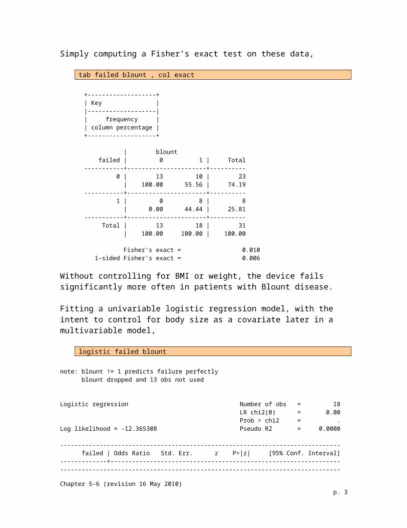
Simply computing a Fisher’s exact test on these data,
tab failed blount , col exact
+-------------------+| Key ||-------------------|| frequency || column percentage |+-------------------+
| blount failed | 0 1 | Total-----------+----------------------+---------- 0 | 13 10 | 23 | 100.00 55.56 | 74.19 -----------+----------------------+---------- 1 | 0 8 | 8 | 0.00 44.44 | 25.81 -----------+----------------------+---------- Total | 13 18 | 31 | 100.00 100.00 | 100.00
Fisher's exact = 0.010 1-sided Fisher's exact = 0.006
Without controlling for BMI or weight, the device fails significantly more often in patients with Blount disease.
Fitting a univariable logistic regression model, with the intent to control for body size as a covariate later in a multivariable model,
logistic failed blount
note: blount != 1 predicts failure perfectly blount dropped and 13 obs not used
Logistic regression Number of obs = 18 LR chi2(0) = 0.00 Prob > chi2 = .Log likelihood = -12.365308 Pseudo R2 = 0.0000
------------------------------------------------------------------------------ failed | Odds Ratio Std. Err. z P>|z| [95% Conf. Interval]-------------+----------------------------------------------------------------------------------------------------------------------------------------------
We discover that a logistic regression model cannot be fitted to these data. Perhaps this is what Schroerlucke et al (2009) discovered when they attempted to analyze these data, although they never mention it or discuss what statistical methods were used.
What is happening here, and how to model such data, is the subject of this chapter.
Chapter 5-6 (revision 16 May 2010) p. 2
Maximum Likelihood Estimation
In linear regression, we found the values of regression coefficients that described a line of best fit through the data using the method of least squares. We did this by finding the line that minimized the deviations of the observed values from the predicted values.
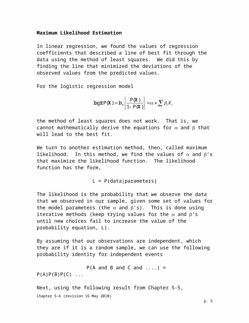
For the logistic regression model
P( )logit P( ) ln
1 P( )e i iX
XX
X
the method of least squares does not work. That is, we cannot mathematically derive the equations for and that will lead to the best fit.
We turn to another estimation method, then, called maximum likelihood. In this method, we find the values of and ’s that maximize the likelihood function. The likelihood function has the form,
L = P(data|parameters)
The likelihood is the probability that we observe the data that we observed in our sample, given some set of values for the model parameters (the and ’s). This is done using iterative methods (keep trying values for the and ’s until new choices fail to increase the value of the probability equation, L).
By assuming that our observations are independent, which they are if it is a random sample, we can use the following probability identity for independent events
P(A and B and C and ....) = P(A)P(B)P(C) ...
Next, using the following result from Chapter 5-5,
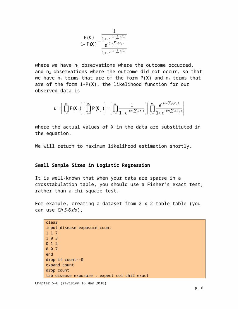
where we have n1 observations where the outcome occurred, and n2 observations where the outcome did not occur, so that we have n1 terms that are of the form P(X) and n2 terms that are of the form 1-P(X), the likelihood function for our observed data is
where the actual values of X in the data are substituted in the equation.Chapter 5-6 (revision 16 May 2010)
p. 3
We will return to maximum likelihood estimation shortly.
Small Sample Sizes in Logistic Regression
It is well-known that when your data are sparse in a crosstabulation table, you should use a Fisher’s exact test, rather than a chi-square test.
For example, creating a dataset from 2 x 2 table table (you can use Ch 5-6.do),
clearinput disease exposure count1 1 71 0 30 1 20 0 7enddrop if count==0expand countdrop counttab disease exposure , expect col chi2 exact
+--------------------+| Key ||--------------------|| frequency || expected frequency || column percentage |+--------------------+
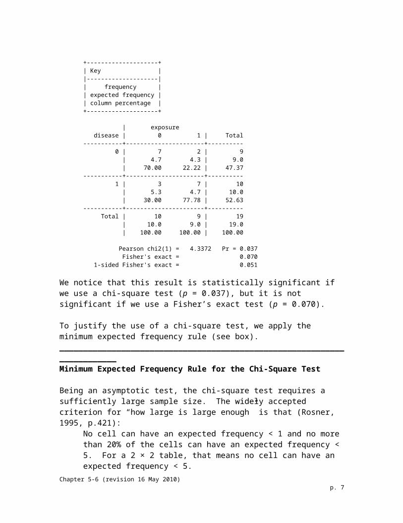
| exposure disease | 0 1 | Total-----------+----------------------+---------- 0 | 7 2 | 9 | 4.7 4.3 | 9.0 | 70.00 22.22 | 47.37 -----------+----------------------+---------- 1 | 3 7 | 10 | 5.3 4.7 | 10.0 | 30.00 77.78 | 52.63 -----------+----------------------+---------- Total | 10 9 | 19 | 10.0 9.0 | 19.0 | 100.00 100.00 | 100.00
Pearson chi2(1) = 4.3372 Pr = 0.037 Fisher's exact = 0.070 1-sided Fisher's exact = 0.051
We notice that this result is statistically significant if we use a chi-square test (p = 0.037), but it is not significant if we use a Fisher’s exact test (p = 0.070).
To justify the use of a chi-square test, we apply the minimum expected frequency rule (see box).
Chapter 5-6 (revision 16 May 2010) p. 4
________________________________________________________________________Minimum Expected Frequency Rule for the Chi-Square Test
Being an asymptotic test, the chi-square test requires a sufficiently large sample size. The widely accepted criterion for “how large is large enough” is that (Rosner, 1995, p.421):
No cell can have an expected frequency < 1 and no more than 20% of the cells can have an expected frequency < 5. For a 2 × 2 table, that means no cell can have an expected frequency < 5.
Altman (1991, p.253) relaxes this somewhat, but no many people are aware of Altman’s perspective:
In practice this rule can be relaxed for a 2 × 2 table to allow one cell to have an expected value slightly lower than 5.
The expected frequency of a contingency table cell is calculated as expected cell frequency = (row total × column total) / grand total.
(See Ch 2-4, “Minimum Expected Frequency Rule for Using Chi-Square Test” , p.18 for a more detailed description of this rule of thumb.)________________________________________________________________________
Example The minimum expected frequency rule is well-known and widely used. For example, Cuchel et al. (2007) state in the Statistical Analysis section of their article,
“Percentages were analyzed using the chi-square test or Fisher’s exact test when expected cell counts were less than 5.”
Returning to the above example, we observe that three (75%) of the cells have an expected frequency < 5, and so the chi-square test is not appropriate.
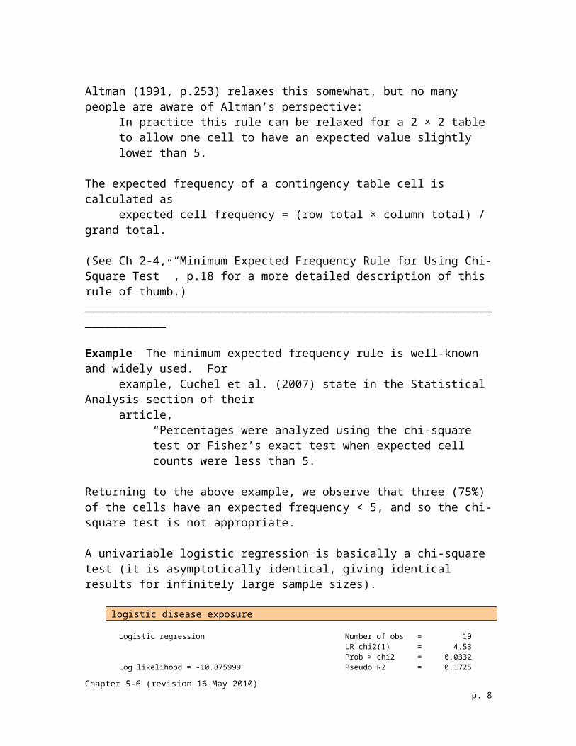
A univariable logistic regression is basically a chi-square test (it is asymptotically identical, giving identical results for infinitely large sample sizes).
logistic disease exposure
Logistic regression Number of obs = 19 LR chi2(1) = 4.53 Prob > chi2 = 0.0332Log likelihood = -10.875999 Pseudo R2 = 0.1725
------------------------------------------------------------------------------ disease | Odds Ratio Std. Err. z P>|z| [95% Conf. Interval]-------------+---------------------------------------------------------------- exposure | 8.166667 8.639103 1.99 0.047 1.027074 64.93634------------------------------------------------------------------------------
Chapter 5-6 (revision 16 May 2010) p. 5
This compares with the above crosstabulation analysis,
Pearson chi2(1) = 4.3372 Pr = 0.037
in that the crosstabulation chi-square test and the logistic regression test on the “exposure” coefficient (called the Wald test) are both significant. With the larger sample size example in the previous chapter, the p values were essentially identical.
This raises an interesting question. If we do a crosstabulation analysis and fail to get significance because we were required to use the Fisher’s exact test, is it okay to switch to logistic regression?
This is actually a question regarding the adequacy of maximum likelihood (ML) estimation for small sample sizes. (see box)
ML estimators with small samples
Long and Freese (2006, p.77) explain,
“Although ML estimators are not necessarily bad estimators in small samples, the small-sample behavior of ML estimators for the models we consider is largely unknown. Except for the logit and Poisson regression, which can be fitted using exact permutation methods with LogXact (Cytel Corporation 2005), alternative estimators with known small-sample properties are generally not available. With this in mind, Long (1997, 54) proposed the following guidelines for the use of ML in small samples:
It is risky to use ML with samples smaller than 100, while samples over 500 seem adequate. These values should be raised depending on characteristics of the model and the data. First, if there are many parameters, more observations are needed…. A rule of at least 10 observations per parameter seems reasonable…. This does not imply that a minimum of 100 is not needed if you have only two parameters. Second, if the data are ill-conditioned (e.g., independent variables are highly collinear) or if there is little variation in the dependent variable (e.g., nealry all the outcomes are 1), a larger sample is required. Third, some models seem to require more observations (such as the ordinal regression model or the zero-inflated count models).”
_______________ Long, JS. (1997). Regression Models for Categorical and Limited Dependent Variables,
vol. 7 of Advanced Quantitative Techniques in the Social Sciences. Thousand Oakes, CA: Sage.
The only solution to a small sample size is to resort to exact logistic regression, for many years available only in the LogXact software. Since LogXact has not been widely used, researchers and statisticians have historically basically just ignored the problem. Now, however, exact logistic regression is available in popular statistical packages such as SAS Chapter 5-6 (revision 16 May 2010)
p. 6
and Stata (beginning with Stata version 10), so the use of exact logistic regression is becoming more common.
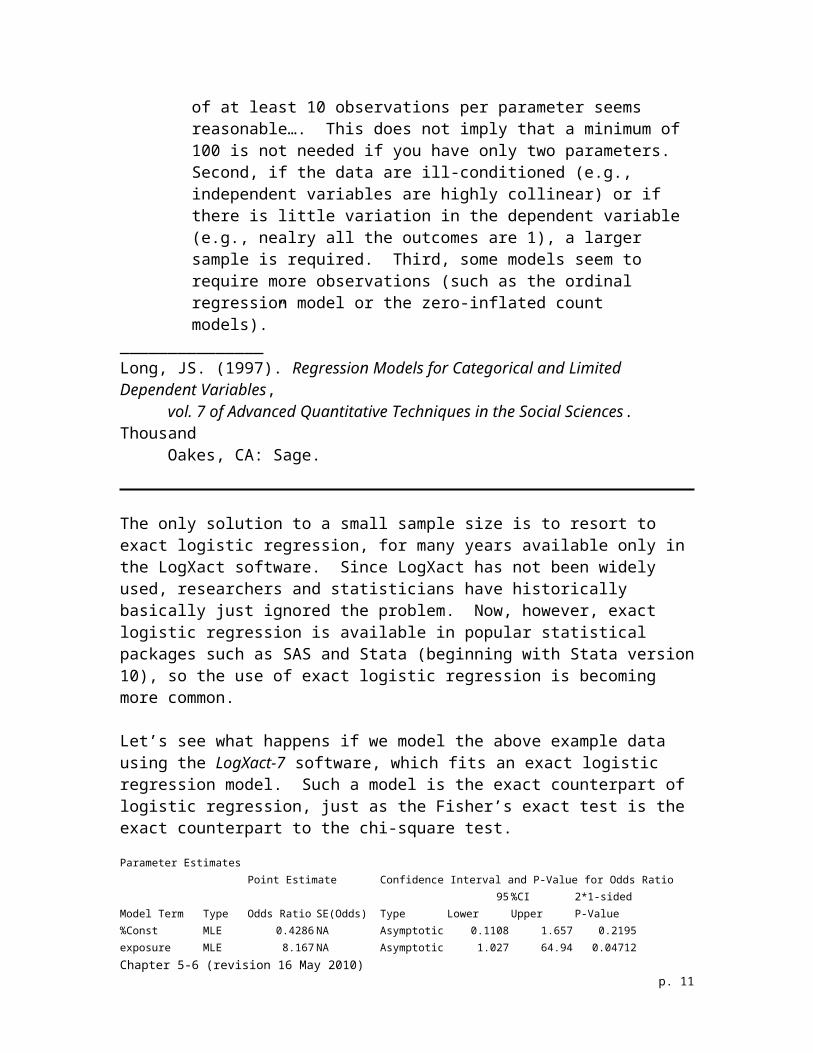
Let’s see what happens if we model the above example data using the LogXact-7 software, which fits an exact logistic regression model. Such a model is the exact counterpart of logistic regression, just as the Fisher’s exact test is the exact counterpart to the chi-square test.
Parameter EstimatesPoint Estimate Confidence Interval and P-Value for Odds Ratio
95 %CI 2*1-sidedModel Term Type Odds Ratio SE(Odds) Type Lower Upper P-Value%Const MLE 0.4286 NA Asymptotic 0.1108 1.657 0.2195exposure MLE 8.167 NA Asymptotic 1.027 64.94 0.04712
CMLE 7.166 NA Exact 0.752 113.4 0.1025
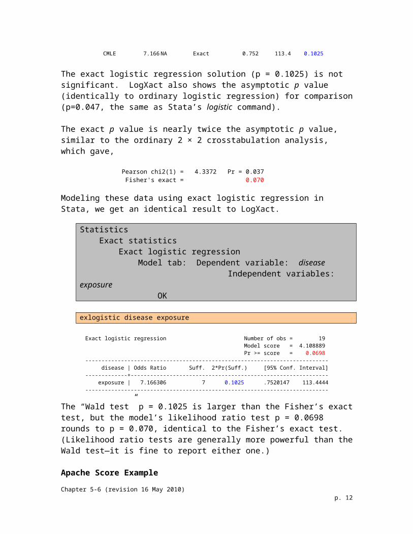
The exact logistic regression solution (p = 0.1025) is not significant. LogXact also shows the asymptotic p value (identically to ordinary logistic regression) for comparison (p=0.047, the same as Stata’s logistic command).
The exact p value is nearly twice the asymptotic p value, similar to the ordinary 2 × 2 crosstabulation analysis, which gave,
Pearson chi2(1) = 4.3372 Pr = 0.037 Fisher's exact = 0.070
Modeling these data using exact logistic regression in Stata, we get an identical result to LogXact.
Statistics Exact statistics Exact logistic regression Model tab: Dependent variable: disease Independent variables: exposure OK
exlogistic disease exposure
Exact logistic regression Number of obs = 19 Model score = 4.108889 Pr >= score = 0.0698--------------------------------------------------------------------------- disease | Odds Ratio Suff. 2*Pr(Suff.) [95% Conf. Interval]-------------+------------------------------------------------------------- exposure | 7.166306 7 0.1025 .7520147 113.4444---------------------------------------------------------------------------
The “Wald test” p = 0.1025 is larger than the Fisher’s exact test, but the model’s likelihood ratio test p = 0.0698 rounds to p = 0.070, identical to the Fisher’s exact test. (Likelihood ratio tests are generally more powerful than the Wald test—it is fine to report either one.)
Chapter 5-6 (revision 16 May 2010) p. 7
Apache Score Example
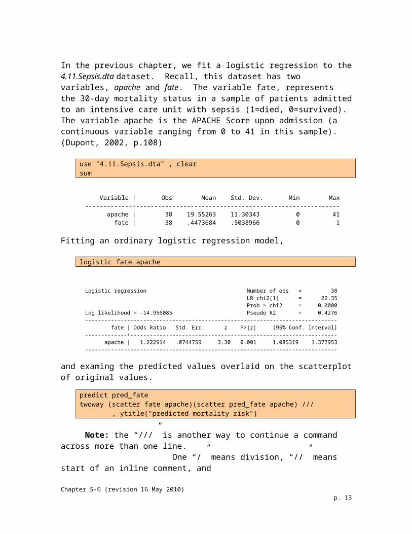
In the previous chapter, we fit a logistic regression to the 4.11.Sepsis.dta dataset. Recall, this dataset has two variables, apache and fate. The variable fate, represents the 30-day mortality status in a sample of patients admitted to an intensive care unit with sepsis (1=died, 0=survived). The variable apache is the APACHE Score upon admission (a continuous variable ranging from 0 to 41 in this sample). (Dupont, 2002, p.108)
use "4.11.Sepsis.dta" , clearsum
Variable | Obs Mean Std. Dev. Min Max-------------+-------------------------------------------------------- apache | 38 19.55263 11.30343 0 41 fate | 38 .4473684 .5038966 0 1
Fitting an ordinary logistic regression model,
logistic fate apache
Logistic regression Number of obs = 38 LR chi2(1) = 22.35 Prob > chi2 = 0.0000Log likelihood = -14.956085 Pseudo R2 = 0.4276------------------------------------------------------------------------------ fate | Odds Ratio Std. Err. z P>|z| [95% Conf. Interval]-------------+---------------------------------------------------------------- apache | 1.222914 .0744759 3.30 0.001 1.085319 1.377953------------------------------------------------------------------------------
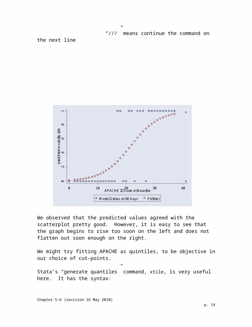
and examing the predicted values overlaid on the scatterplot of original values.
predict pred_fatetwoway (scatter fate apache)(scatter pred_fate apache) /// , ytitle("predicted mortality risk")
Note: the “///” is another way to continue a command across more than one line. One “/” means division, “//” means start of an inline comment, and “///” means continue the command on the next line
Chapter 5-6 (revision 16 May 2010) p. 8

0.2
.4.6
.81
pred
icte
d m
orta
lity
risk
0 10 20 30 40APACHE II Score at Baseline
Mortal Status at 30 Days Pr(fate)
We observed that the predicted values agreed with the scatterplot pretty good. However, it is easy to see that the graph begins to rise too soon on the left and does not flatten out soon enough on the right.
We might try fitting APACHE as quintiles, to be objective in our choice of cut-points.
Stata’s “generate quantiles” command, xtile, is very useful here. It has the syntax:
xtile new_variable_name = orginal_variable_name , nq(5) where the “nq” options is “number of quantiles”. Specifying 5 gives quintiles.
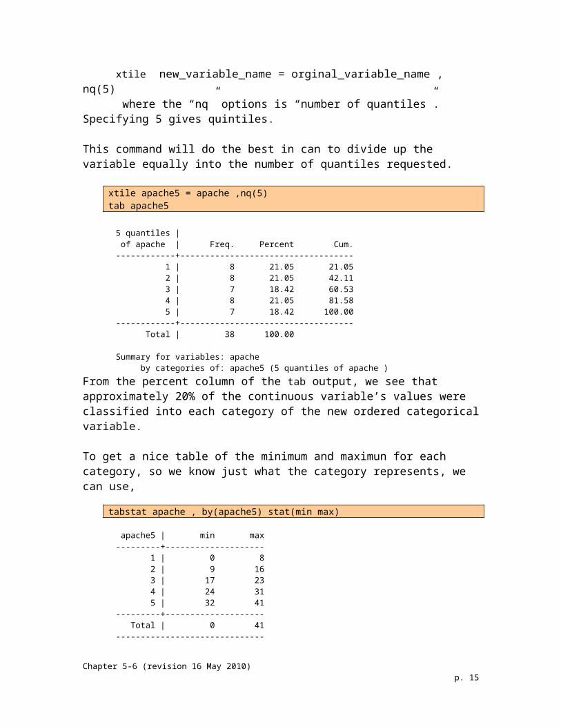
This command will do the best in can to divide up the variable equally into the number of quantiles requested.
xtile apache5 = apache ,nq(5)tab apache5
5 quantiles | of apache | Freq. Percent Cum.------------+----------------------------------- 1 | 8 21.05 21.05 2 | 8 21.05 42.11 3 | 7 18.42 60.53 4 | 8 21.05 81.58 5 | 7 18.42 100.00------------+----------------------------------- Total | 38 100.00
Summary for variables: apache by categories of: apache5 (5 quantiles of apache )
Chapter 5-6 (revision 16 May 2010) p. 9
From the percent column of the tab output, we see that approximately 20% of the continuous variable’s values were classified into each category of the new ordered categorical variable.
To get a nice table of the minimum and maximun for each category, so we know just what the category represents, we can use,
tabstat apache , by(apache5) stat(min max)
apache5 | min max---------+-------------------- 1 | 0 8 2 | 9 16 3 | 17 23 4 | 24 31 5 | 32 41---------+-------------------- Total | 0 41------------------------------
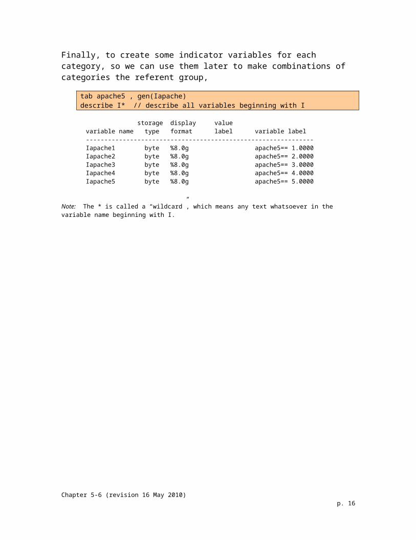
Finally, to create some indicator variables for each category, so we can use them later to make combinations of categories the referent group,
tab apache5 , gen(Iapache)describe I* // describe all variables beginning with I
storage display valuevariable name type format label variable label--------------------------------------------------------------Iapache1 byte %8.0g apache5== 1.0000Iapache2 byte %8.0g apache5== 2.0000Iapache3 byte %8.0g apache5== 3.0000Iapache4 byte %8.0g apache5== 4.0000Iapache5 byte %8.0g apache5== 5.0000
Note: The * is called a “wildcard”, which means any text whatsoever in the variable name beginning with I.
Chapter 5-6 (revision 16 May 2010) p. 10
Stata Version 10:
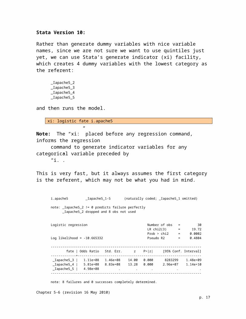
Rather than generate dummy variables with nice variable names, since we are not sure we want to use quintiles just yet, we can use Stata’s generate indicator (xi) facility, which creates 4 dummy variables with the lowest category as the referent:
_Iapache5_2 _Iapache5_3 _Iapache5_4 _Iapache5_5
and then runs the model.
xi: logistic fate i.apache5
Note: The “xi:” placed before any regression command, informs the regression command to generate indicator variables for any categorical variable preceded by “i.”.
This is very fast, but it always assumes the first category is the referent, which may not be what you had in mind.
i.apache5 _Iapache5_1-5 (naturally coded; _Iapache5_1 omitted)
note: _Iapache5_2 != 0 predicts failure perfectly _Iapache5_2 dropped and 8 obs not used
Logistic regression Number of obs = 30 LR chi2(3) = 19.72 Prob > chi2 = 0.0002Log likelihood = -10.665332 Pseudo R2 = 0.4804
------------------------------------------------------------------------------ fate | Odds Ratio Std. Err. z P>|z| [95% Conf. Interval]-------------+---------------------------------------------------------------- _Iapache5_3 | 1.11e+08 1.46e+08 14.00 0.000 8283299 1.48e+09 _Iapache5_4 | 5.81e+08 8.83e+08 13.28 0.000 2.96e+07 1.14e+10 _Iapache5_5 | 4.98e+08 . . . . .------------------------------------------------------------------------------
note: 8 failures and 0 successes completely determined.
The “xi:” in the command “xi: logistic fate i.apache5” dropped the first quintile to use as the referent group, which is why we see the message _Iapache5_1 omitted
This model is a complete disaster.
Chapter 5-6 (revision 16 May 2010) p. 11
Stata Version 11:
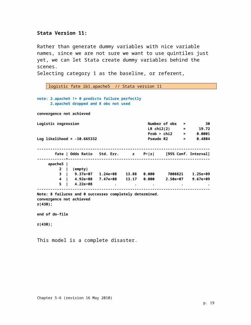
Rather than generate dummy variables with nice variable names, since we are not sure we want to use quintiles just yet, we can let Stata create dummy variables behind the scenes.Selecting category 1 as the baseline, or referent,
logistic fate ib1.apache5 // Stata version 11
note: 2.apache5 != 0 predicts failure perfectly 2.apache5 dropped and 8 obs not used
convergence not achieved
Logistic regression Number of obs = 30 LR chi2(2) = 19.72 Prob > chi2 = 0.0001Log likelihood = -10.665332 Pseudo R2 = 0.4804
------------------------------------------------------------------------------ fate | Odds Ratio Std. Err. z P>|z| [95% Conf. Interval]-------------+---------------------------------------------------------------- apache5 | 2 | (empty) 3 | 9.37e+07 1.24e+08 13.88 0.000 7008821 1.25e+09 4 | 4.92e+08 7.47e+08 13.17 0.000 2.50e+07 9.67e+09 5 | 4.22e+08 . . . . .------------------------------------------------------------------------------Note: 8 failures and 0 successes completely determined.convergence not achievedr(430);
end of do-file
r(430);
This model is a complete disaster.
Chapter 5-6 (revision 16 May 2010) p. 12
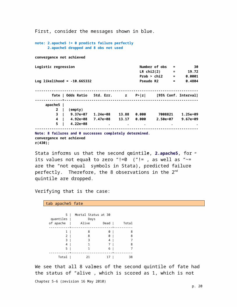
First, consider the messages shown in blue.
note: 2.apache5 != 0 predicts failure perfectly 2.apache5 dropped and 8 obs not used
convergence not achieved
Logistic regression Number of obs = 30 LR chi2(2) = 19.72 Prob > chi2 = 0.0001Log likelihood = -10.665332 Pseudo R2 = 0.4804
------------------------------------------------------------------------------ fate | Odds Ratio Std. Err. z P>|z| [95% Conf. Interval]-------------+---------------------------------------------------------------- apache5 | 2 | (empty) 3 | 9.37e+07 1.24e+08 13.88 0.000 7008821 1.25e+09 4 | 4.92e+08 7.47e+08 13.17 0.000 2.50e+07 9.67e+09 5 | 4.22e+08 . . . . .------------------------------------------------------------------------------Note: 8 failures and 0 successes completely determined.convergence not achievedr(430);
Stata informs us that the second quintile, 2.apache5, for its values not equal to zero “!=0” (“!=”, as well as “~=” are the “not equal” symbols in Stata), predicted failure perfectly. Therefore, the 8 observations in the 2nd quintile are dropped.
Verifying that is the case:
tab apache5 fate
5 | Mortal Status at 30 quantiles | Daysof apache | Alive Dead | Total-----------+----------------------+---------- 1 | 8 0 | 8 2 | 8 0 | 8 3 | 3 4 | 7 4 | 1 7 | 8 5 | 1 6 | 7 -----------+----------------------+---------- Total | 21 17 | 38
We see that all 8 values of the second quintile of fate had the status of “alive”, which is scored as 1, which is not equal to zero. From this crosstabulation table, we see that no deaths occurred for the second quintile.
Chapter 5-6 (revision 16 May 2010) p. 13
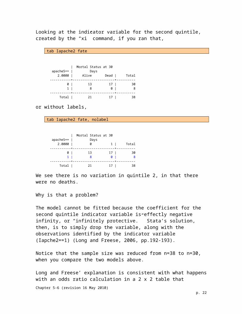
Looking at the indicator variable for the second quintile, created by the “xi” command, if you ran that,
tab Iapache2 fate
| Mortal Status at 30 apache5== | Days 2.0000 | Alive Dead | Total-----------+----------------------+---------- 0 | 13 17 | 30 1 | 8 0 | 8 -----------+----------------------+---------- Total | 21 17 | 38
or without labels,
tab Iapache2 fate, nolabel
| Mortal Status at 30 apache5== | Days 2.0000 | 0 1 | Total-----------+----------------------+---------- 0 | 13 17 | 30 1 | 8 0 | 8 -----------+----------------------+---------- Total | 21 17 | 38
We see there is no variation in quintile 2, in that there were no deaths.
Why is that a problem?
The model cannot be fitted because the coefficient for the second quintile indicator variable is effectly negative infinity, or “infinitely protective.” Stata’s solution, then, is to simply drop the variable, along with the observations identified by the indicator variable (Iapche2==1) (Long and Freese, 2006, pp.192-193).
Notice that the sample size was reduced from n=38 to n=30, when you compare the two models above.
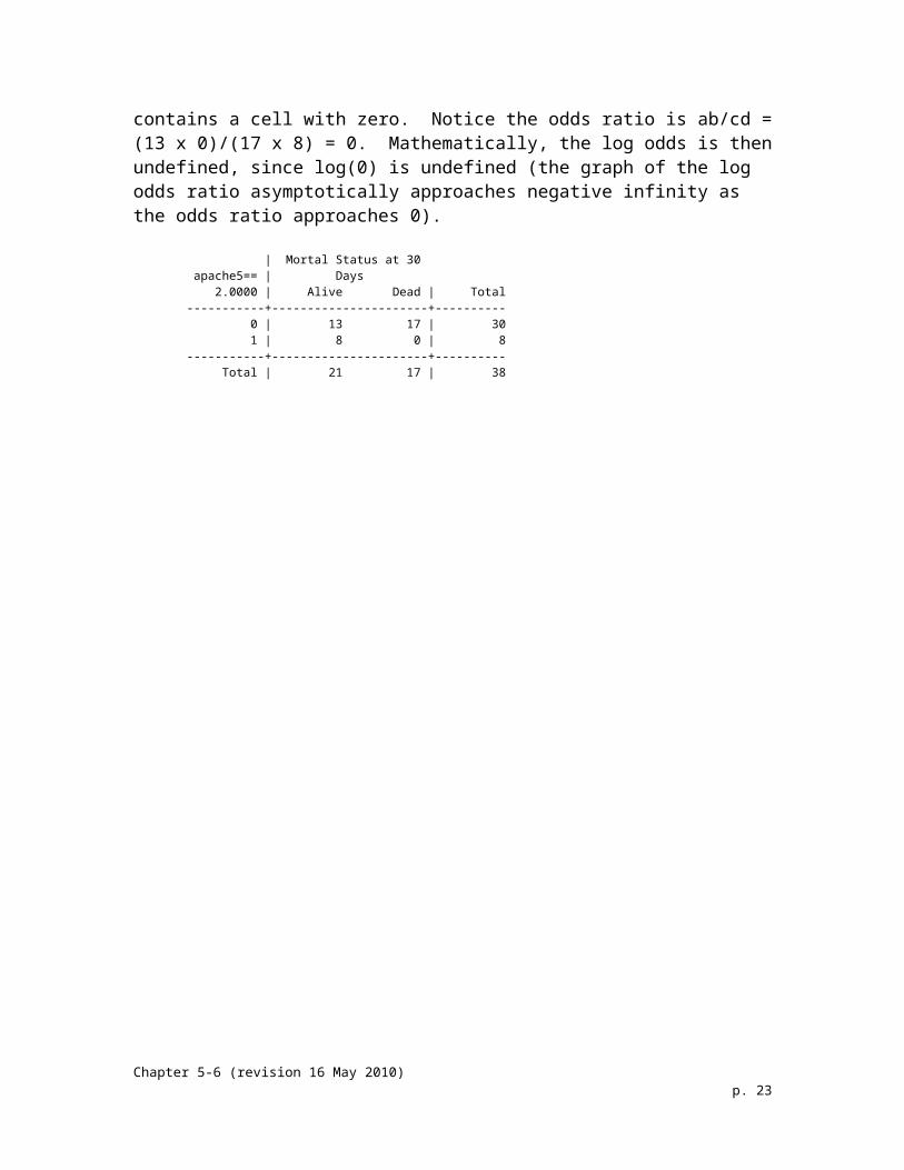
Long and Freese’ explanation is consistent with what happens with an odds ratio calculation in a 2 x 2 table that contains a cell with zero. Notice the odds ratio is ab/cd = (13 x 0)/(17 x 8) = 0. Mathematically, the log odds is then undefined, since log(0) is undefined (the graph of the log odds ratio asymptotically approaches negative infinity as the odds ratio approaches 0).
| Mortal Status at 30 apache5== | Days 2.0000 | Alive Dead | Total-----------+----------------------+---------- 0 | 13 17 | 30 1 | 8 0 | 8 -----------+----------------------+---------- Total | 21 17 | 38
Chapter 5-6 (revision 16 May 2010) p. 14
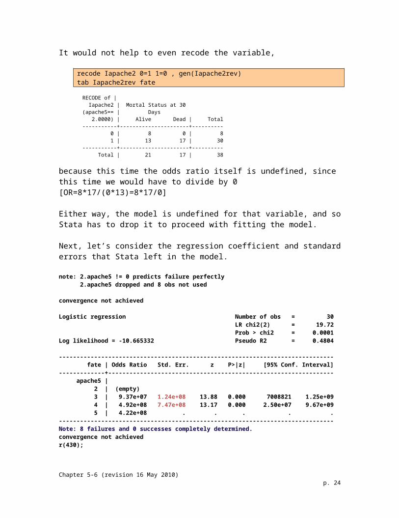
It would not help to even recode the variable,
recode Iapache2 0=1 1=0 , gen(Iapache2rev)tab Iapache2rev fate
RECODE of | Iapache2 | Mortal Status at 30(apache5== | Days 2.0000) | Alive Dead | Total-----------+----------------------+---------- 0 | 8 0 | 8 1 | 13 17 | 30 -----------+----------------------+---------- Total | 21 17 | 38
because this time the odds ratio itself is undefined, since this time we would have to divide by 0 [OR=8*17/(0*13)=8*17/0]
Either way, the model is undefined for that variable, and so Stata has to drop it to proceed with fitting the model.
Next, let’s consider the regression coefficient and standard errors that Stata left in the model.
note: 2.apache5 != 0 predicts failure perfectly 2.apache5 dropped and 8 obs not used
convergence not achieved
Logistic regression Number of obs = 30 LR chi2(2) = 19.72 Prob > chi2 = 0.0001Log likelihood = -10.665332 Pseudo R2 = 0.4804
------------------------------------------------------------------------------ fate | Odds Ratio Std. Err. z P>|z| [95% Conf. Interval]-------------+---------------------------------------------------------------- apache5 | 2 | (empty) 3 | 9.37e+07 1.24e+08 13.88 0.000 7008821 1.25e+09 4 | 4.92e+08 7.47e+08 13.17 0.000 2.50e+07 9.67e+09 5 | 4.22e+08 . . . . .------------------------------------------------------------------------------Note: 8 failures and 0 successes completely determined.convergence not achievedr(430);
Chapter 5-6 (revision 16 May 2010) p. 15
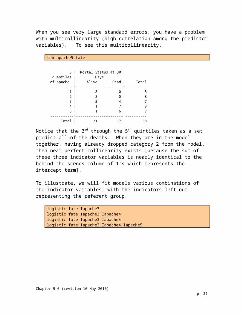
When you see very large standard errors, you have a problem with multicollinearity (high correlation among the predictor variables). To see this multicollinearity,
tab apache5 fate
5 | Mortal Status at 30 quantiles | Daysof apache | Alive Dead | Total-----------+----------------------+---------- 1 | 8 0 | 8 2 | 8 0 | 8 3 | 3 4 | 7 4 | 1 7 | 8 5 | 1 6 | 7 -----------+----------------------+---------- Total | 21 17 | 38
Notice that the 3rd through the 5th quintiles taken as a set predict all of the deaths. When they are in the model together, having already dropped category 2 from the model, then near perfect collinearity exists [because the sum of these three indicator variables is nearly identical to the behind the scenes column of 1’s which represents the intercept term].
To illustrate, we will fit models various combinations of the indicator variables, with the indicators left out representing the referent group.
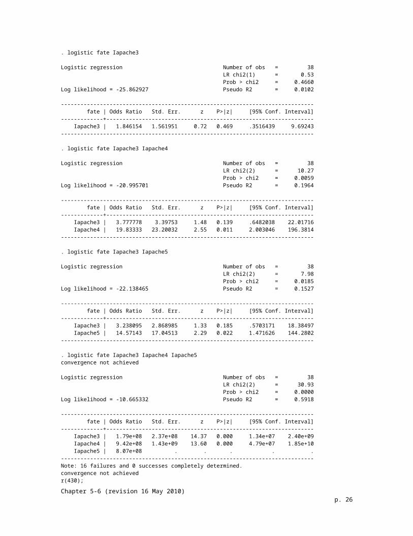
logistic fate Iapache3logistic fate Iapache3 Iapache4logistic fate Iapache3 Iapache5logistic fate Iapache3 Iapache4 Iapache5
Chapter 5-6 (revision 16 May 2010) p. 16
. logistic fate Iapache3
Logistic regression Number of obs = 38 LR chi2(1) = 0.53 Prob > chi2 = 0.4660Log likelihood = -25.862927 Pseudo R2 = 0.0102
------------------------------------------------------------------------------ fate | Odds Ratio Std. Err. z P>|z| [95% Conf. Interval]-------------+---------------------------------------------------------------- Iapache3 | 1.846154 1.561951 0.72 0.469 .3516439 9.69243------------------------------------------------------------------------------
. logistic fate Iapache3 Iapache4
Logistic regression Number of obs = 38 LR chi2(2) = 10.27 Prob > chi2 = 0.0059Log likelihood = -20.995701 Pseudo R2 = 0.1964
------------------------------------------------------------------------------ fate | Odds Ratio Std. Err. z P>|z| [95% Conf. Interval]-------------+---------------------------------------------------------------- Iapache3 | 3.777778 3.39753 1.48 0.139 .6482038 22.01716 Iapache4 | 19.83333 23.20032 2.55 0.011 2.003046 196.3814------------------------------------------------------------------------------
. logistic fate Iapache3 Iapache5
Logistic regression Number of obs = 38 LR chi2(2) = 7.98 Prob > chi2 = 0.0185Log likelihood = -22.138465 Pseudo R2 = 0.1527
------------------------------------------------------------------------------ fate | Odds Ratio Std. Err. z P>|z| [95% Conf. Interval]-------------+---------------------------------------------------------------- Iapache3 | 3.238095 2.868985 1.33 0.185 .5703171 18.38497 Iapache5 | 14.57143 17.04513 2.29 0.022 1.471626 144.2802------------------------------------------------------------------------------
. logistic fate Iapache3 Iapache4 Iapache5convergence not achieved
Logistic regression Number of obs = 38 LR chi2(2) = 30.93 Prob > chi2 = 0.0000Log likelihood = -10.665332 Pseudo R2 = 0.5918
------------------------------------------------------------------------------ fate | Odds Ratio Std. Err. z P>|z| [95% Conf. Interval]-------------+---------------------------------------------------------------- Iapache3 | 1.79e+08 2.37e+08 14.37 0.000 1.34e+07 2.40e+09 Iapache4 | 9.42e+08 1.43e+09 13.60 0.000 4.79e+07 1.85e+10 Iapache5 | 8.07e+08 . . . . .------------------------------------------------------------------------------Note: 16 failures and 0 successes completely determined.convergence not achievedr(430);
We see that the model converged on a solution until we got to the point where the three indicators, taken as a set, identified all of the death cases.
This is an issue with maximum likelihood estimation, which cannot fit the logistic model when perfect, or nearly perfect, discrimination is achieved.
Chapter 5-6 (revision 16 May 2010) p. 17

When Maximum Likelihood Will Fail Completely
There are some datasets for which maximum likelihood estimates do not even exist. This occurs if there is complete separation or quasi-complete separation.
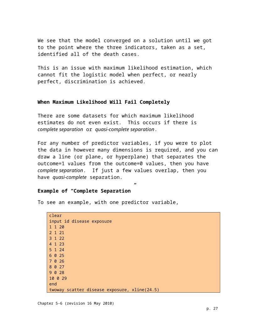
For any number of predictor variables, if you were to plot the data in however many dimensions is required, and you can draw a line (or plane, or hyperplane) that separates the outcome=1 values from the outcome=0 values, then you have complete separation. If just a few values overlap, then you have quasi-complete separation.
Example of “Complete Separation”
To see an example, with one predictor variable,
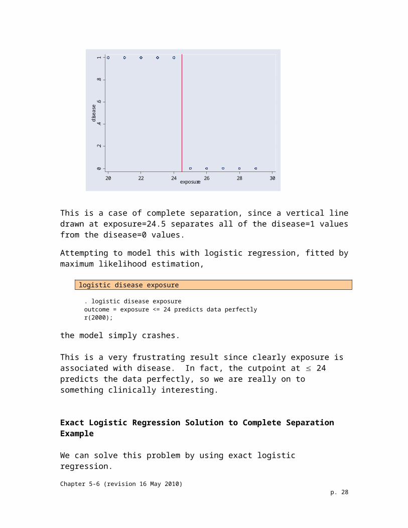
clearinput id disease exposure1 1 202 1 213 1 224 1 235 1 246 0 257 0 268 0 279 0 2810 0 29endtwoway scatter disease exposure, xline(24.5)
0.2
.4.6
.81
dise
ase
20 22 24 26 28 30exposure
This is a case of complete separation, since a vertical line drawn at exposure=24.5 separates all of the disease=1 values from the disease=0 values.
Chapter 5-6 (revision 16 May 2010) p. 18
Attempting to model this with logistic regression, fitted by maximum likelihood estimation,
logistic disease exposure
. logistic disease exposureoutcome = exposure <= 24 predicts data perfectlyr(2000);
the model simply crashes.
This is a very frustrating result since clearly exposure is associated with disease. In fact, the cutpoint at 24 predicts the data perfectly, so we are really on to something clinically interesting.
Exact Logistic Regression Solution to Complete Separation Example
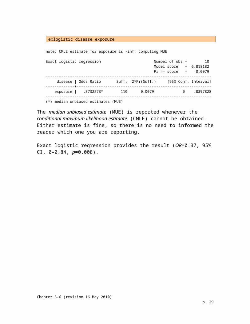
We can solve this problem by using exact logistic regression.
exlogistic disease exposure
note: CMLE estimate for exposure is -inf; computing MUE
Exact logistic regression Number of obs = 10 Model score = 6.818182 Pr >= score = 0.0079--------------------------------------------------------------------------- disease | Odds Ratio Suff. 2*Pr(Suff.) [95% Conf. Interval]-------------+------------------------------------------------------------- exposure | .3732273* 110 0.0079 0 .8397828---------------------------------------------------------------------------(*) median unbiased estimates (MUE)
The median unbiased estimate (MUE) is reported whenever the conditional maximum likelihood estimate (CMLE) cannot be obtained. Either estimate is fine, so there is no need to informed the reader which one you are reporting.
Exact logistic regression provides the result (OR=0.37, 95% CI, 0-0.84, p=0.008).
Chapter 5-6 (revision 16 May 2010) p. 19
Example of “Quasi-Complete Separation”
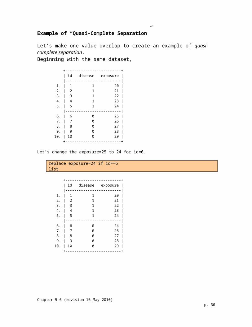
Let’s make one value overlap to create an example of quasi-complete separation.Beginning with the same dataset,
+-------------------------+ | id disease exposure | |-------------------------| 1. | 1 1 20 | 2. | 2 1 21 | 3. | 3 1 22 | 4. | 4 1 23 | 5. | 5 1 24 | |-------------------------| 6. | 6 0 25 | 7. | 7 0 26 | 8. | 8 0 27 | 9. | 9 0 28 | 10. | 10 0 29 | +-------------------------+
Let’s change the exposure=25 to 24 for id=6.
replace exposure=24 if id==6list
+-------------------------+ | id disease exposure | |-------------------------| 1. | 1 1 20 | 2. | 2 1 21 | 3. | 3 1 22 | 4. | 4 1 23 | 5. | 5 1 24 | |-------------------------| 6. | 6 0 24 | 7. | 7 0 26 | 8. | 8 0 27 | 9. | 9 0 28 | 10. | 10 0 29 | +-------------------------+
Chapter 5-6 (revision 16 May 2010) p. 20

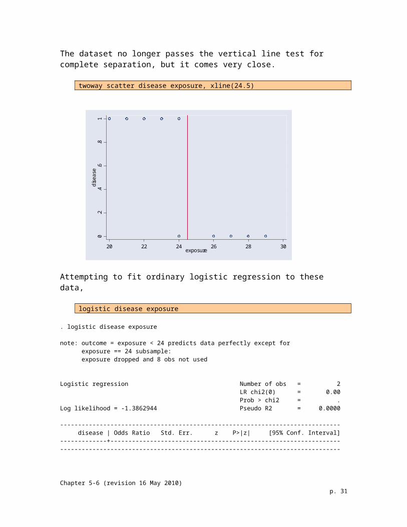
The dataset no longer passes the vertical line test for complete separation, but it comes very close.
twoway scatter disease exposure, xline(24.5)
0.2
.4.6
.81
dise
ase
20 22 24 26 28 30exposure
Attempting to fit ordinary logistic regression to these data,
logistic disease exposure
. logistic disease exposure
note: outcome = exposure < 24 predicts data perfectly except for exposure == 24 subsample: exposure dropped and 8 obs not used
Logistic regression Number of obs = 2 LR chi2(0) = 0.00 Prob > chi2 = .Log likelihood = -1.3862944 Pseudo R2 = 0.0000
------------------------------------------------------------------------------ disease | Odds Ratio Std. Err. z P>|z| [95% Conf. Interval]-------------+----------------------------------------------------------------------------------------------------------------------------------------------
The ordinary logistic regression model could still could not be fit.
The exact logistic model can be fit, however.
Chapter 5-6 (revision 16 May 2010) p. 21
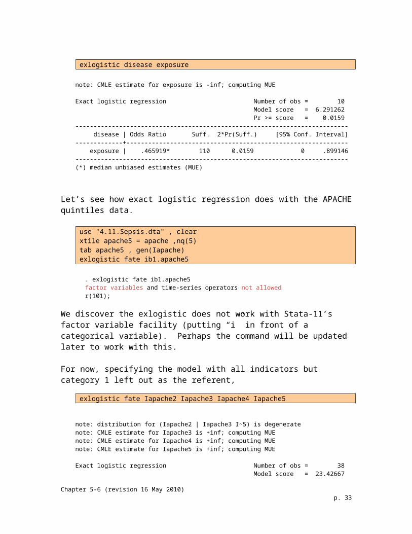
exlogistic disease exposure
note: CMLE estimate for exposure is -inf; computing MUE
Exact logistic regression Number of obs = 10 Model score = 6.291262 Pr >= score = 0.0159--------------------------------------------------------------------------- disease | Odds Ratio Suff. 2*Pr(Suff.) [95% Conf. Interval]-------------+------------------------------------------------------------- exposure | .465919* 110 0.0159 0 .899146---------------------------------------------------------------------------(*) median unbiased estimates (MUE)
Let’s see how exact logistic regression does with the APACHE quintiles data.
use "4.11.Sepsis.dta" , clearxtile apache5 = apache ,nq(5)tab apache5 , gen(Iapache)exlogistic fate ib1.apache5
. exlogistic fate ib1.apache5factor variables and time-series operators not allowedr(101);
We discover the exlogistic does not work with Stata-11’s factor variable facility (putting “i” in front of a categorical variable). Perhaps the command will be updated later to work with this.
For now, specifying the model with all indicators but category 1 left out as the referent,
exlogistic fate Iapache2 Iapache3 Iapache4 Iapache5
note: distribution for (Iapache2 | Iapache3 I~5) is degeneratenote: CMLE estimate for Iapache3 is +inf; computing MUEnote: CMLE estimate for Iapache4 is +inf; computing MUEnote: CMLE estimate for Iapache5 is +inf; computing MUE
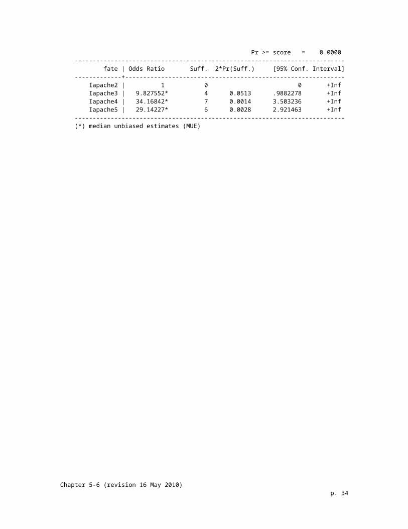
Exact logistic regression Number of obs = 38 Model score = 23.42667 Pr >= score = 0.0000--------------------------------------------------------------------------- fate | Odds Ratio Suff. 2*Pr(Suff.) [95% Conf. Interval]-------------+------------------------------------------------------------- Iapache2 | 1 0 0 +Inf Iapache3 | 9.827552* 4 0.0513 .9882278 +Inf Iapache4 | 34.16842* 7 0.0014 3.503236 +Inf Iapache5 | 29.14227* 6 0.0028 2.921463 +Inf---------------------------------------------------------------------------(*) median unbiased estimates (MUE)
Chapter 5-6 (revision 16 May 2010) p. 22
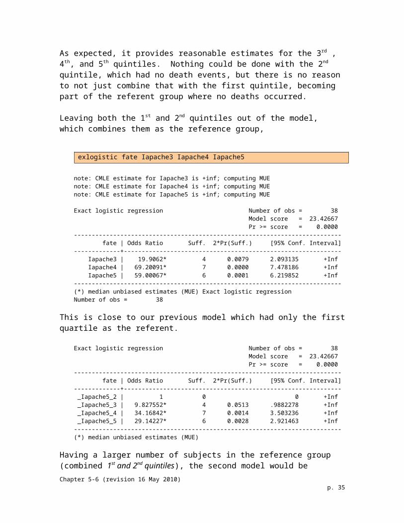
As expected, it provides reasonable estimates for the 3rd , 4th, and 5th quintiles. Nothing could be done with the 2nd quintile, which had no death events, but there is no reason to not just combine that with the first quintile, becoming part of the referent group where no deaths occurred.
Leaving both the 1st and 2nd quintiles out of the model, which combines them as the reference group,
exlogistic fate Iapache3 Iapache4 Iapache5
note: CMLE estimate for Iapache3 is +inf; computing MUEnote: CMLE estimate for Iapache4 is +inf; computing MUEnote: CMLE estimate for Iapache5 is +inf; computing MUE
Exact logistic regression Number of obs = 38 Model score = 23.42667 Pr >= score = 0.0000--------------------------------------------------------------------------- fate | Odds Ratio Suff. 2*Pr(Suff.) [95% Conf. Interval]-------------+------------------------------------------------------------- Iapache3 | 19.9062* 4 0.0079 2.093135 +Inf Iapache4 | 69.20091* 7 0.0000 7.478186 +Inf Iapache5 | 59.00067* 6 0.0001 6.219852 +Inf---------------------------------------------------------------------------(*) median unbiased estimates (MUE) Exact logistic regression Number of obs = 38
This is close to our previous model which had only the first quartile as the referent.
Exact logistic regression Number of obs = 38 Model score = 23.42667 Pr >= score = 0.0000--------------------------------------------------------------------------- fate | Odds Ratio Suff. 2*Pr(Suff.) [95% Conf. Interval]-------------+------------------------------------------------------------- _Iapache5_2 | 1 0 0 +Inf _Iapache5_3 | 9.827552* 4 0.0513 .9882278 +Inf _Iapache5_4 | 34.16842* 7 0.0014 3.503236 +Inf _Iapache5_5 | 29.14227* 6 0.0028 2.921463 +Inf---------------------------------------------------------------------------(*) median unbiased estimates (MUE)
Having a larger number of subjects in the reference group (combined 1st and 2nd quintiles), the second model would be considered more reliable. Notice the confidence intervals are tighter, lower bound further from zero, in the model with the combined 1st and 2nd quintiles.
Chapter 5-6 (revision 16 May 2010) p. 23
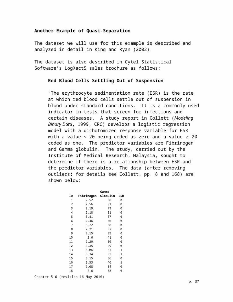
Another Example of Quasi-Separation
The dataset we will use for this example is described and analyzed in detail in King and Ryan (2002).
The dataset is also described in Cytel Statistical Software’s LogXact5 sales brochure as follows:
Red Blood Cells Settling Out of Suspension
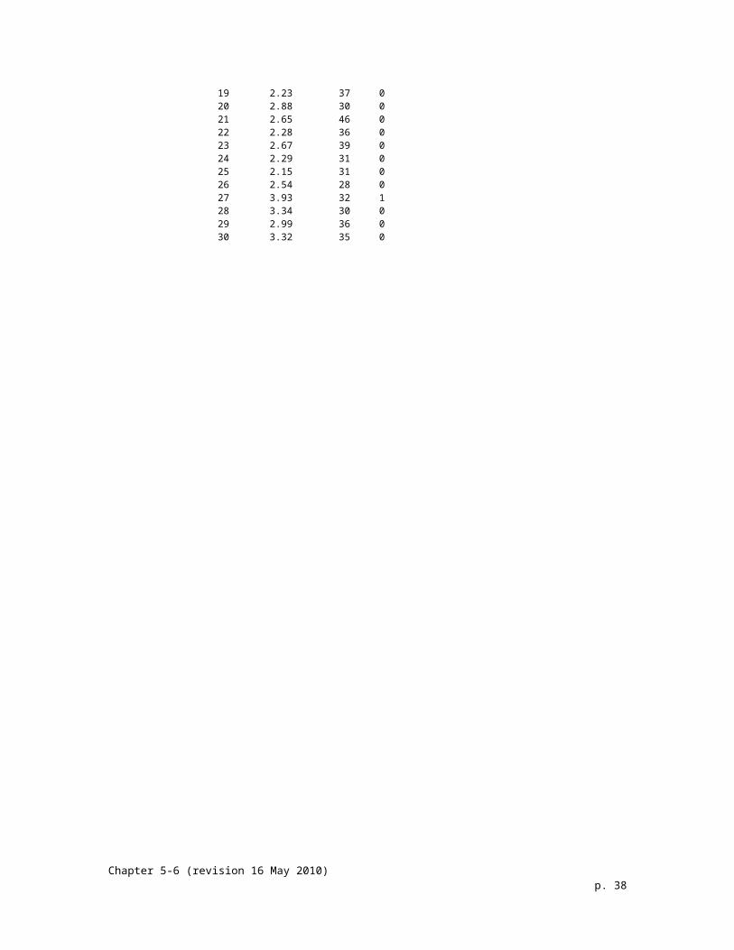
“The erythrocyte sedimentation rate (ESR) is the rate at which red blood cells settle out of suspension in blood under standard conditions. It is a commonly used indicator in tests that screen for infections and certain diseases. A study report in Collett (Modeling Binary Data, 1999, CRC) develops a logistic regression model with a dichotomized response variable for ESR with a value < 20 being coded as zero and a value 20 coded as one. The predictor variables are Fibrinogen and Gamma globulin. The study, carried out by the Institute of Medical Research, Malaysia, sought to determine if there is a relationship between ESR and the predictor variables. The data (after removing outliers; for details see Collett, pp. 8 and 168) are shown below:
Gamma ID Fibrinogen Globulin ESR 1 2.52 38 0 2 2.56 31 0 3 2.19 33 0 4 2.18 31 0 5 3.41 37 0 6 2.46 36 0 7 3.22 38 0 8 2.21 37 0 9 3.15 39 0 10 2.6 41 0 11 2.29 36 0 12 2.35 29 0 13 5.06 37 1 14 3.34 32 1 15 3.15 36 0 16 3.53 46 1 17 2.68 34 0 18 2.6 38 0 19 2.23 37 0 20 2.88 30 0 21 2.65 46 0 22 2.28 36 0 23 2.67 39 0 24 2.29 31 0 25 2.15 31 0 26 2.54 28 0 27 3.93 32 1 28 3.34 30 0 29 2.99 36 0 30 3.32 35 0
Chapter 5-6 (revision 16 May 2010) p. 24
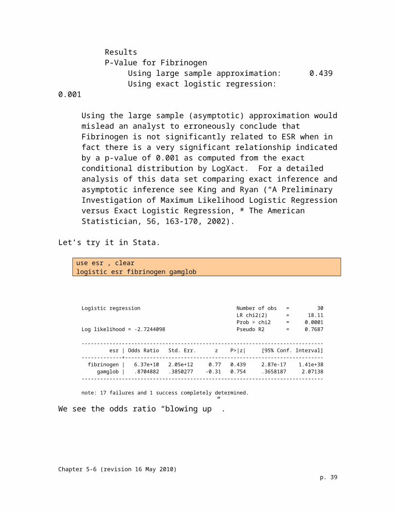
ResultsP-Value for Fibrinogen
Using large sample approximation: 0.439 Using exact logistic regression: 0.001
Using the large sample (asymptotic) approximation would mislead an analyst to erroneously conclude that Fibrinogen is not significantly related to ESR when in fact there is a very significant relationship indicated by a p-value of 0.001 as computed from the exact conditional distribution by LogXact. For a detailed analysis of this data set comparing exact inference and asymptotic inference see King and Ryan (“A Preliminary Investigation of Maximum Likelihood Logistic Regression versus Exact Logistic Regression, “ The American Statistician, 56, 163-170, 2002).”
Let’s try it in Stata.
use esr , clearlogistic esr fibrinogen gamglob
Logistic regression Number of obs = 30 LR chi2(2) = 18.11 Prob > chi2 = 0.0001Log likelihood = -2.7244098 Pseudo R2 = 0.7687
------------------------------------------------------------------------------ esr | Odds Ratio Std. Err. z P>|z| [95% Conf. Interval]-------------+---------------------------------------------------------------- fibrinogen | 6.37e+10 2.05e+12 0.77 0.439 2.87e-17 1.41e+38 gamglob | .8704882 .3850277 -0.31 0.754 .3658187 2.07138------------------------------------------------------------------------------
note: 17 failures and 1 success completely determined.
We see the odds ratio “blowing up” .
Chapter 5-6 (revision 16 May 2010) p. 25
We can graphically observe quasi-separation with fibrinogen,
twoway scatter esr fibrinogen , xline(3.33)
0.2
.4.6
.81
esr
2 3 4 5fibrinogen
Separation is not a problem for gamma globulin,
twoway scatter esr gamglob
Chapter 5-6 (revision 16 May 2010) p. 26
0.2
.4.6
.81
esr
30 35 40 45gamglob
Graphing both variables together,
twoway (scatter fibrinogen gamglob ,mlabel(esr))(pci 3.8 26 3.4 47)
00
00
0
0
0
0
0
0
00
1
1
0
1
00
0
0
0
0
0
00
0
1
0
0
0
23
45
25 30 35 40 45
fibrinogen y/yb
We see that we can draw a diagonal line and only one ESR=1 case will cross over it, suggesting quasi-separation defined by two variables. We can check to see if the “joint” quasi-separation creates the problem by modeling the two variables separately.
logistic esr fibrinogen logistic esr gamglob
. logistic esr fibrinogen
Logistic regression Number of obs = 30 LR chi2(1) = 17.98 Prob > chi2 = 0.0000Log likelihood = -2.7911477 Pseudo R2 = 0.7631------------------------------------------------------------------------------ esr | Odds Ratio Std. Err. z P>|z| [95% Conf. Interval]-------------+---------------------------------------------------------------- fibrinogen | 3.82e+07 5.16e+08 1.29 0.196 .0001238 1.18e+19------------------------------------------------------------------------------note: 9 failures and 1 success completely determined.
. logistic esr gamglob
Logistic regression Number of obs = 30 LR chi2(1) = 0.46 Prob > chi2 = 0.4961Log likelihood = -11.548594 Pseudo R2 = 0.0197
------------------------------------------------------------------------------ esr | Odds Ratio Std. Err. z P>|z| [95% Conf. Interval]-------------+---------------------------------------------------------------- gamglob | 1.08396 .1273327 0.69 0.493 .8610389 1.364596------------------------------------------------------------------------------
Chapter 5-6 (revision 16 May 2010) p. 27
We notice that the estimates do not “blow up” quite as much, but still they blow up too much to provide a useful model.
Note: This example suggests that quasi-separation could be created by a set of variables. This is something to watch for in your own datasets.
Adding an interaction term does not help.
gen fibgam=fibrinogen*gamgloblogistic esr fibrinogen gamglob fibgam
Logistic regression Number of obs = 30 LR chi2(3) = 18.85 Prob > chi2 = 0.0003Log likelihood = -2.3542984 Pseudo R2 = 0.8001
------------------------------------------------------------------------------ esr | Odds Ratio Std. Err. z P>|z| [95% Conf. Interval]-------------+---------------------------------------------------------------- fibrinogen | 2.44e-27 2.03e-25 -0.74 0.462 3.05e-98 1.96e+44 gamglob | .0002056 .0020858 -0.84 0.403 4.75e-13 88962.48 fibgam | 11.30184 32.69964 0.84 0.402 .0389374 3280.44------------------------------------------------------------------------------
The solution is to use exact logistic regression and report its result.
exlogistic esr fibrinogen gamglob
Exact logistic regression Number of obs = 30 Model score = 14.61946 Pr >= score = 0.0004--------------------------------------------------------------------------- esr | Odds Ratio Suff. 2*Pr(Suff.) [95% Conf. Interval]-------------+------------------------------------------------------------- fibrinogen | 12.79579* 15.86 0.0022 2.262284 +Inf gamglob | 1* 147 1.0000 .1601282 +Inf---------------------------------------------------------------------------(*) median unbiased estimates (MUE)
Protocol Suggestion
If you suspect that you will have near or perfect separation, and particularly if you have a sample size < 100, you say something like the following in your protocol,
The outcome will be modeled using logistic regression with potential confoundingvariables included as covariates. Interaction terms will be included to assess effect-measure modification, and then removed if not significant. A graphical assessment of quasi-separation will be performed, as quasi-separation can lead to inaccurate maximum likelihood estimates (King and Ryan, 2002). If quasi-separation is present, the data will be modeled using exact logistic regression (Mehta and Patel, 1995).
Chapter 5-6 (revision 16 May 2010) p. 28
Articles on Exact Logistic Regression
Here are four papers on exact logistic regression:
Ammann, R.A. (2004). Defibrotide for hepatic VOD in children: exact statistics can help! Bone Marrow Transplantation 34: 277-278.
King EN, Ryan TP. (2002). A preliminary investigation of maximum likelihood logistic regression versus exact logistic regression. The American Statistician, 56(3):163-170.
Metha CR, et al (2000). Efficient Monte Carlo methods for conditional logisticregression. J Am Statit Assoc 95(449):99-108.
Bull SB, Mak C, Greenwood CMT. (2002). A modified score function estimator for multinomial logistic regression in small samples. Computational Statistics and Data Analysis. 39:57-74.
Any statistician consulting with a client where exact logistic regression is needed, or any researcher needing to convey the concept to a co-author, should share the Ammann paper, which is a one-page article.
Chapter 5-6 (revision 16 May 2010) p. 29
Overfitting
Overfitting is a common problem in regression models. It is the problem of obtaining unreliable associations, which will not show up in future datasets or patients, due to having too many predictor variables for the number of events or sample size.
This would be a good time to review the topic (see Chapter 2-5, pp.24-31).
Exact Solution to Overfitting
Suppose you want to publish a paper where you have only 10 cases of the disease outcome and you want to fit a logistic regression with four predictor variables. Clearly this will produce an overfitting problem, for which they could be criticized (you need at least 5 cases for every predictor, if the aim is to adjust for confounding, at 10 more or cases if the aim is to develop a prediction model).
Likewise, suppose you wanted to show univariable logistic regression models for which there were zero cases with an exposure for some of our predictor variables, so that the logistic regression model could not be fit at all.
Exact logistic regression would provide a solution to both issues.
Here is a rather lengthy Statistic Methods paragraph, which you could use if the the reviewer came back and asked you to elaborate on the use of exact logistic regression:
“All reported p values, odds ratios, and confidence intervals were obtained using exact logistic regression (LogXact-5 statistical software, Cambridge, MA: Cytel Software Corporation). Ordinary maximum likelihood logistic regression fails when: 1) the data are sparse, such as few outcome events, 2) the number of events divided by the number of predictor variables in the model is small, such as < 10 , or 3) there exists near perfect or perfect separation, where all events occur in one predictor category or the other. In these cases, an ordinary logistic regression model cannot be fit at all, or when it can be fit, the estimates of odds ratios, confidence intervals, and p values are biased. Exact logistic regression, on the other hand, can fit a model and the model estimates are unbiased. (King and Ryan, 2002; Mehta. 2000; Ammann, 2004). Using exact logistic regression, we were able to obtained unbiased estimates in both univariable and multivariable models, even though we only had 12 HHV-6 Positive cases for our primary analysis, and 5 cases in our secondary analysis.”
Look at the above quote and notice the three times that exact logistic regression is indicated.
Chapter 5-6 (revision 16 May 2010) p. 30
Specifically, Mehta, one of the developers of LogXact, specifically stated that exact logistic regression is not affected by the overfitting problem (Mehta, 2000, Introduction paragraph):
“Logistic regression is a popular mathematical model for the analysis of binary data with widespread applicability in the physical, biomedical, and behavioral sciences. Parameter inference for this model is usually based on maximizing the unconditional likelihood function. For large well-balanced datasets or for datasets with only a few parameters, unconditional maximum likelihood inference is a satisfactory approach. However unconditional maximum likelihood inference can produce inconsistent point estimates, inaccurate p values, and inaccurate confidence intervals for small or unbalanced datasets and for datasets with a large number of parameters relative to the number of observations. Sometimes the method fails entirely as no estimates can be found that maximize the unconditional likelihood function. A methodologically sound alternative approach that has none of the aforementioned drawbacks is the exact conditional approach. Here one estimates the parameters of interest by computing the exact permutation distributions of their sufficient statistics, conditional on the observed values of the sufficient statistics for the remaining nuisance parameters.”
Chapter 5-6 (revision 16 May 2010) p. 31
Defining an Odds Ratio When a Cell Has a Zero Count
Sometimes exact logistic regression produces an OR in the opposite direction that you would expect, in the situation when the result is not statistically significant. As an example,
clearinput hhv6 plate count1 1 01 0 50 1 110 0 58enddrop if count==0expand countdrop countexlogistic hhv6 plate*clearinput hhv6 death count1 1 01 0 50 1 50 0 64enddrop if count==0expand countdrop countexlogistic hhv6 death
Exact logistic regression Number of obs = 74 Model score = .9236255 Pr >= score = 0.5932--------------------------------------------------------------------------- hhv6 | Odds Ratio Suff. 2*Pr(Suff.) [95% Conf. Interval]-------------+------------------------------------------------------------- plate | .8200102* 0 0.8727 0 6.579727---------------------------------------------------------------------------(*) median unbiased estimates (MUE)
Exact logistic regression Number of obs = 74 Model score = .3833228 Pr >= score = 1.0000--------------------------------------------------------------------------- hhv6 | Odds Ratio Suff. 2*Pr(Suff.) [95% Conf. Interval]-------------+------------------------------------------------------------- death | 2.045171* 0 1.0000 0 18.28607---------------------------------------------------------------------------(*) median unbiased estimates (MUE)
Chapter 5-6 (revision 16 May 2010) p. 32
Exact logistic regression produced the following non-significant ORs and CIs:
Clinical Variable HHV-6 Positive (n=5)
HHV-6 Negative(n=69)
OR (95% CI)
Platelets < 100,000 0 (0%) 11 (16%) 0.8 (0-6.6)Death before Discharge 0 (0%) 5 (7%) 2.0 (0-18.3)
Given the zero in the cell of the 2 × 2 table that would make the association infinitely protective, it would seem that exact logistic regression would provide an odds ratio < 1.0. It did for one of the associations shown, but not for the other.
Although it can at least provide an odds ratio, which ordinary logistic regression cannot do, exact logistic regression can give these unexpected OR estimates in the non-statistically significant situations of zero cells. The same thing happens with the long-accepted practice of adding ½ to each cell of the 2 × 2 table to avoid zero cell counts. Selvin (2004, p.450) provides Haldane’s (1956) formulas, which are:
with estimated variance
The two odds ratios computed using Haldane’s method are
HHV-6 PositiveYes No
Platelets < 100,000 Yes 0 11No 5 58
OR = (0.5 × 58.5)/(11.5 × 5.5) = 0.46and
HHV-6 PositiveYes No
Death before Discharge Yes 0 5No 5 64
OR = (0.5 × 64.5)/(5.5 × 5.5) = 1.07
Chapter 5-6 (revision 16 May 2010) p. 33
Case Study: Schroerlucke Dataset
Returning to the case study, where ordinary logistic regression could not be fitted,we can fit the univariable exact logistic model.
After reading in the dataset, schroerlucke.dta, we fit the model without covariates, using
exlogistic failed blount
note: CMLE estimate for blount is +inf; computing MUE
Exact logistic regression Number of obs = 31 Model score = 7.536232 Pr >= score = 0.0096--------------------------------------------------------------------------- failed | Odds Ratio Suff. 2*Pr(Suff.) [95% Conf. Interval]-------------+------------------------------------------------------------- blount | 12.48967* 8 0.0111 1.655921 +Inf---------------------------------------------------------------------------(*) median unbiased estimates (MUE)
Next, adjusting for weight,
exlogistic failed blount weight
note: CMLE estimate for blount is +inf; computing MUE
Exact logistic regression Number of obs = 31 Model score = 7.65015 Pr >= score = 0.0178--------------------------------------------------------------------------- failed | Odds Ratio Suff. 2*Pr(Suff.) [95% Conf. Interval]-------------+------------------------------------------------------------- blount | 8.495888* 8 0.0600 .9205344 +Inf weight | 1.01012 762.3 0.7005 .9613036 1.064392---------------------------------------------------------------------------(*) median unbiased estimates (MUE)
It appears that Schroerlucke et al concluded the right thing, that Blount disease increases the risk for the screw breakages, after controlling for the patient’s weight.
Two things would need to be argued: 1) Having up to two implants on the same patient did not require something special to account for a potential lack of independence in the data. We will return to this later in the course after we have covered the topic of clustered sampling.2) It is okay to conclude an effect with a p value slightly larger than 0.05. An argument for this is found in Chapter 2-13, p.5.
Chapter 5-6 (revision 16 May 2010) p. 34
Appendix. Exact Logistic Regression Using SAS (included here in case your co-investigators are SAS users)
Exact logistic regression can also be computed in SAS, which is a widely used statistical software package. How to do this will be demonstrated using the complete separation example from page 13.
0.2
.4.6
.81
dise
ase
20 22 24 26 28 30exposure
These data are in the Excel file, “complete separation.xls”.
id disease exposure1 1 202 1 213 1 224 1 235 1 246 0 257 0 268 0 279 0 28
10 0 29
To read this Excel file into SAS, copy the following into the SAS Editor window and hit the run button (the toolbar icon that looks like a little man running).
PROC IMPORT OUT= WORK.DATA1 DATAFILE= "C:\Documents and Settings\u0032770.SRVR\Desktop\regressionclass\datasets & do-files\complete separation.xls" DBMS=EXCEL REPLACE; SHEET="Sheet1$"; GETNAMES=YES;RUN;
Chapter 5-6 (revision 16 May 2010) p. 35

Note: The DATEFILE line is very sensitive to embedded spaces. Notice that the continuation of the line must begin at the left margin. If you add spaces or tab over, it will think those spaces or tab is part of the directory path and then give you an error message because it cannot find the file.
To run an ordinary logistic regression, copy the following into the Editor window, highlight it, and hit the run botton.
proc logistic descending data=work.data1; model disease=exposure;run;
Note: By default, the logistic procedure in SAS thinks the outcome event is scored as 0 (0=disease, 1= not disease). Always be sure to include the word “descending” after “logistic”, as shown here, for the outcome event to be scored as 1 (1=disease, 0 = not disease). SAS confirms your choice but displaying the following in the Log window when you run this block of commands:
NOTE: PROC LOGISTIC is modeling the probability that disease=1.
When you run this block of commands, you get the following warning in the Log window:
WARNING: There is a complete separation of data points. The maximum likelihood estimate does not exist.WARNING: The LOGISTIC procedure continues in spite of the above warning. Results shown are based on the last maximum likelihood iteration. Validity of the model fit is questionable.
In the SAS Output window, you see the result:
The LOGISTIC ProcedureWARNING: The validity of the model fit is questionable.
Analysis of Maximum Likelihood Estimates
Standard Wald Parameter DF Estimate Error Chi-Square Pr > ChiSq Intercept 1 247.0 433.7 0.3244 0.5690 exposure 1 -10.0824 17.6974 0.3246 0.5689
Odds Ratio Estimates Point 95% Wald Effect Estimate Confidence Limits exposure <0.001 <0.001 >999.999
Whereas Stata simply crashes and gives an error message, SAS gives outputs a model that sort of looks valid, but actually blows up (OR <0.001, 95% CI, <0.001 - >999.999).
Chapter 5-6 (revision 16 May 2010) p. 36
To fit an exact logistic regression, use the following:
proc logistic descending data=work.data1; model disease=exposure; exact exposure/estimate=both;run;
Since we specified “/estimate=both”, we get the ordinary logistic regression followed by the exact logistic regression. The exact logistic regression from the Output window is:
Exact Conditional Analysis Conditional Exact Tests
Exact Odds Ratios 95% Confidence Parameter Estimate Limits p-Value exposure 0.373* 0 0.840 0.0079 NOTE: * indicates a median unbiased estimate.
This result agrees exact with LogXact-7, from page 14:
Parameter EstimatesPoint Estimate Confidence Interval and P-Value for Odds Ratio
95 %CI 2*1-sidedModel Term Type Odds Ratio SE(Odds) Type Lower Upper P-Value%Const MLE ? ? Asymptotic ? ? ?exposure MLE ? ? Asymptotic ? ? ?
MUE 0.3732 NA Exact 0 0.8398 0.007937
Chapter 5-6 (revision 16 May 2010) p. 37
As an enhancement, to get nicely formatted output in SAS, add the following lines:
ods pdf;ods graphics on;proc logistic descending data=work.data1; model disease=exposure; exact exposure/estimate=both;run;ods graphics off;ods pdf close;
Not only is the output in nice looking tables, but it is in pdf format, which can be saved as a pdf file.
Chapter 5-6 (revision 16 May 2010) p. 38
References
Ammann, R.A. (2004). Defibrotide for hepatic VOD in children: exact statistics can help! Bone Marrow Transplantation 34: 277-278.
Altman DG. (1991). Practical Statistics for Medical Research. New York, Chapman & Hall/CRC.
Cuchel M, Bledon LT, Szapary PO, et al. (2007). Inhibition of microsmal triglyceride transfer protein in familial hypercholesterolemia. N Engl J Med 356:148-56.
Dupont WD. (2002). Statistical Modeling for Biomedical Researchers: a Simple Introduction to the Analysis of Complex Data. Cambridge, Cambridge University Press.
Haldane JBS. (1956). The estimation and significance of logarithm of a ratio offrequencies. Annals of Human Genetics 20:309-11.
King EN, Ryan TP. (2002). A preliminary investigation of maximum likelihood logistic regression versus exact logistic regression. The American Statistician, 56(3):163-170.
Long JS, Freese J. (2006). Regression models for categorical dependent variables using Stata. 2nd edition. College Station TX, Stata Press.
Mehta CR, Patel NR. (1995). Exact logistic regression: theory and examples. Statistics in Medicine 14:2143-2160.
Metha CR, et al (2000). Efficient Monte Carlo methods for conditional logisticregression. J Am Statit Assoc 95(449):99-108.
Rosner B. (1995). Fundamentals of Biostatistics, 4th ed. Belmont CA, Duxbury Press.
Schroerlucke S, Bertrand S, Clapp J, et al. (2009). Failure of orthofix eight-plate for the treatment of blount disease. J Pediatr Orthop 29(1):57-60.
Selvin S. (2004). Statistical Analysis of Epidemiologic Data. 3rd ed. New York, OxfordUniversity Press.
Chapter 5-6 (revision 16 May 2010) p. 39