1

The Total Asset Growth Anomaly: Is It Incremental to the Net

Operating Asset Growth Anomaly?

S. Sean Cao1

shuncao2@uiuc.edu

Department of Accountancy

College of Business

284 Wohlers Hall

University of Illinois at Urbana-Champaign

1206 S. Sixth Street

Champaign IL 61820.

1 I am indebted to my dissertation chair, Gans Narayanamoorthy and the members of my dissertation

committee, Wei Li, Scott Weisbenner and Martin Wu for their invaluable time and guidance. I thank

Theodore Sougiannis, Jay Wang and empirical seminar participants at the University of Illinois for their

insightful comments and suggestions.

2

The Total Asset Growth Anomaly: Is It Incremental to the Net

Operating Asset Growth Anomaly?

ABSTRACT

This study documents that the total asset (TA) growth anomaly (Cooper et al.

2008) is a noisy manifestation of the net operating asset (NOA) growth anomaly

documented in earlier accounting literature. To better understand the underlying causes of

the growth anomalies, I decompose TA growth into NOA growth and two additional

components. Out of the three components, the TA growth anomaly appears to be driven

primarily by the market’s misunderstanding of NOA growth’s negative implications for

future profitability. The two additional components fail to predict future abnormal returns

and, in fact, substantially dilute the predictability of NOA growth. To demonstrate the

economic significance of using the correct growth anomaly proxy, I show that TA growth

and NOA growth have differential robustness to market-friction controls. This study

suggests that not all asset growth components contribute to a ―growth anomaly‖ and that

the financing sources of asset growth need to receive greater attention in studies of

growth anomalies.

Keywords: growth anomalies; total asset growth; net operating asset growth; market

mispricing

Data Availability: All data are from public sources

3

I. INTRODUCTION

An expanding body of literature explores a ―growth effect‖ on future abnormal

returns. The underlying empirical regularity is that asset growth (e.g., acquisitions;

capital investment; debt and equity offerings) tends to be anomalously followed by

periods of negative abnormal returns.2 In a seminal paper, Cooper et al. (2008) introduce

total asset (TA) growth strategy as a new growth anomaly and argue that TA growth is

the strongest determinant of future negative returns relative to all previously documented

growth components. This new anomaly has received great attention, spawning a new line

of research that seeks to explain its anomalous returns. These studies are divided

between offering behavioral or risk-based explanations for the anomaly (e.g., Chen and

Zhang 2009; Chan et al. 2008). However, none of these studies can completely explain

the abnormal negative returns of TA growth, and the cause of the TA growth anomaly

remains puzzling. In addition, Cooper et al.’s (2008) research inspired a sequence of

studies to examine whether this ―new‖ anomaly exists in global financial markets, such as

the Pacific-Basin region and Australia (e.g., Chen, Yao and Yu 2010; Gray and Johnson

2010).

Prior to the research of Cooper et al. (2008), Fairfield et al. (2003) introduced a

growth anomaly using growth in net operating assets (NOA). Fairfield et al. (2003) argue

that NOA growth captures the effect of diminishing marginal returns from investment

growth (Stigler 1963), thus negatively effecting future profitability. They show that the

2 Examples include Asquith 1983, Spiess and Affleck-Graves 1999, Richardson and Sloan 2003, and

Titman et al. 2004.

4

market fails to understand the negative implications of NOA growth for future

profitability in a timely fashion. Abnormal negative returns are earned in subsequent

periods when the market learns of the negative implications. While both the TA and the

NOA growth anomalies have been investigated separately in great depth, no study has

systemically examined the relation between these two phenomena. In this paper, I

investigate whether a new influential anomaly, the TA growth anomaly, provides

incremental predictive power for future negative returns over and above the NOA growth

anomaly documented in earlier accounting literature.

If the TA growth anomaly is highly related to NOA growth, the explanation

established for the NOA growth anomaly will be helpful in identifying the underlying

causes of the TA growth anomaly and contribute to the current on-going debate about

behavioral versus risk-based explanations. Reconciling these two anomalies will also

simplify future research that follows the two growth anomalies.

Based on regression and portfolio analyses, I find that Cooper et al.’s (2008) TA

growth anomaly is completely subsumed by the NOA growth anomaly. In contrast, the

predictive power of NOA growth in future negative returns remains the same (-8 to -13

percent) across all TA growth partitions. The results are robust to using both equal-

weighted (EW) and value-weighted (VW) portfolio returns. To investigate the

subsumption of Cooper et al.’s (2008) new anomaly and better understand its causes, I

decompose TA growth into three subparts: 1) growth in operating assets financed by

growth in debt and equity (i.e., NOA growth); 2) growth in operating assets financed by

growth in operating liabilities (hereafter, OAOL); and 3) growth in cash and marketable

securities (hereafter, CASH). The result that the NOA growth anomaly subsumes the TA

5

growth anomaly suggests that the two additional components (growth in CASH and

OAOL) likely provide no incremental power in predicting future negative returns over

NOA growth. The empirical results support this explanation. The two additional

components, in fact, dilute the abnormal negative returns of the NOA growth strategy by

28 (29.7) percent and reduce the t-statistics by 36 (38) percent for EW (VW) portfolios.

Out of the three subcomponents of TA growth, NOA growth is the only driver of TA

growth’s future negative returns. In summary, the newly influential TA growth anomaly

found in the finance literature appears to be a noisy manifestation of the NOA growth

anomaly documented in earlier accounting literature.

Given no study has yet completely explained the abnormal returns of the TA

growth anomaly, an important implication of the finding that the TA growth anomaly is

subsumed by NOA growth anomaly is to test whether the explanation established for the

NOA growth anomaly can apply to the TA growth strategy, I, thus, investigate the effects

of TA growth and its three subcomponents on firms’ future profitability and the market’s

understanding of these effects. Consistent with prior literature (Fairfield et al. 2003;

Richardson et al. 2005), NOA growth has strong negative implications for future

profitability, while the other two components do not. The results from the Mishkin (1983)

test suggest that the market perceives that asset growth has non-negative implications for

future profitability, similar to the findings of Fairfield et al. (2003) and related studies.3

The inability of the market to incorporate the negative implications of NOA growth leads

to abnormal negative returns in subsequent periods. However, the market is able to

3 The market tends to respond favorably to announcements of capital investment increases. Several studies

find that announcements of capital investments increases are, on average, associated with significant

positive excess stock returns (McConnell and Muscarella 1985;Blose and Shieh 1997; Vogt 1997)

6

correctly incorporate the non-negative implications of the two additional components of

TA growth into price. As a result, the two additional components fail to predict future

abnormal returns and, in fact, dilute the predictability of the major forecasting driver—

NOA growth. In sum, out of the three subcomponents, the abnormal negative returns of

the TA growth anomaly are driven by the market’s misunderstanding of the negative

implications only associated with NOA growth. This paper, thus, corroborates Fairfield et

al.’s (2003) finding that stock prices fail to reflect the negative implications of NOA

growth and extend their study by showing that the market can correctly price the non-

negative implications of growth in CASH and OAOL.

I demonstrate the economic significance of using the correct growth anomaly

proxy by showing that TA and NOA growth have differential robustness to arbitrage risk.

Lam and Wei (2010) and Lipson et al. (2009) use TA growth as the ―growth effect‖

measure and find that the abnormal returns following TA growth are not robust to

arbitrage risk. They, thus, argue that the ―growth effect‖ can be explained by arbitrage

risk. I replicate their studies using NOA growth and TA growth. While the TA growth

anomaly generates no abnormal returns in the lowest arbitrage risk portfolio, the NOA

growth strategy still lead to statistically significant negative returns when arbitrage risk is

absent/low. This result demonstrates that using the correct growth anomaly measure leads

to a different result.

This paper provides researchers with prescriptions regarding both explaining the

―growth effect‖ and controlling for it. The results show that not all growth components

contribute to the ―growth effect‖ (e.g., growth in CASH and OAOL). The types of assets

that are growing (e.g., CASH vs. Operating Assets) do matter. Most importantly, this

7

paper shows that in studies of investigating the ―growth effect‖, researchers should pay

more attention to the financing sources of asset growth (e.g., NOA vs. OAOL).

Additionally, as demonstrated by the differential results with respect to arbitrage risk

discussed earlier, researchers are likely better off using NOA growth rather than TA

growth when controlling for the ―growth effect.‖ I close this paper with robustness tests

and a discussion of whether the superior predictive power that NOA growth has in

relation to TA growth is due to additional risk exposure of NOA growth.

The remainder of the paper proceeds according to the following format. In

Section II, I review related literatures and describe the decomposition of TA growth.

Section III describes the data, along with variable definitions and presents empirical

results. Section IV provides concluding remarks.

II. BACKGROUD

This section first provides a review of the TA and NOA growth anomalies. Next, I

illustrate the relevance of this study in relation to the long line of studies that compare

anomalies. Finally, I discuss the decomposition of TA growth into NOA growth and the

additional components.

The TA and NOA Growth Anomalies

Prior research has documented that an increase in firms’ investment has predictive

power for future negative returns. Titman et al. (2004) find evidence of negative returns

8

following large increases in capital expenditures, while Spies and Affleck-Graves (1999)

find that debt offerings, like equity offerings (Ibbotson 1975; Loughran and Ritter 1995),

predict future negative returns. Cooper et al. (2008) contribute to this line of research by

providing a new and comprehensive measure of the ―growth effect.‖ They argue that TA

growth is the strongest determinant of future returns, with a t-statistic twice the size of

that obtained by other growth variables previously documented in the literature.

This new anomaly measure has spawned a new line of research to explain its

abnormal returns. For risk-based explanations, Chen and Zhang (2009) apply q-theory

and construct an investment factor to explain the anomalous returns. While the

investment factor successfully explains other anomalies, such as the momentum anomaly

and the financial distress anomaly, the TA growth anomaly remains robust to the

investment factor. In a working paper, Chan et al. (2008) also attempt to investigate and

distinguish possible mispricing explanations (e.g., the agency cost hypothesis, the

extrapolation hypothesis and the M&A hypothesis). However, none of these studies is

able to completely explain the abnormal negative returns of TA growth; the cause of the

TA growth anomaly remains puzzling.

Prior to the research of Cooper et al. (2008), Fairfield et al. (2003) argue that

NOA growth captures the effect of diminishing marginal returns from investment

growth (Stigler 1963) and reflects the nature of accounting conservatism. It leads NOA

growth to have negative implications on one-year-ahead ROA. These two, however, are

not the only reasons hypothesized for the negative implications that NOA growth has

for future profitability. Richardson et al. (2005, 2006) argue that accounting distortion

(e.g., accrual and earnings reversal) can also lead to decreased future profitability

9

following NOA growth.4 While debate continues as to the reasons for NOA growth’s

negative implications, as far as this study is concerned, a consensus has emerged that

NOA growth has negative implications on future ROA. 5

Literature Comparing Anomalies

This study is related to a long line of anomaly studies that seek to identify

similarities and differences in various documented anomalies and uses the methodologies

employed in these studies (e.g., Collin and Hribar 2000; Desai et al. 2004; Cheng et al.

2006; Chordia and Shivakumar 2006). Collin and Hribar (2000) investigate a possible

relation between accrual anomaly and post-earnings announcement drift. They conclude

that the two anomalies are distinct from each other through two-way sorting portfolio

analyses and the Mishkin test. In a similar fashion, Chordia and Shivakumar (2006) find

that price momentum is subsumed by post-earnings announcement drift (i.e., earnings

momentum) and argue that price momentum is driven by the systematic component of

earnings momentum. As for the TA and NOA growth anomalies, while these two

phenomena have been investigated separately in great depth, no study has systemically

examined the relation between the two, despite both belonging to the family of growth in

accounting numbers.

4 Note that the NOA growth anomaly focuses on the extreme deciles. 5 In contrast to NOA growth, several studies suggest that the implications of the additional two components

(i.e., growth in CASH and OAOL) for future probability or abnormal returns are non-negative (Biais and

Gollier 1997; Long et al. 1994; Richardson et al. 2005 ; Keynes 1936; Palazzo 2010;Chan et al. 2008)

10

Empirical analyses of whether one anomaly can subsume another are not always

clear-cut. For instance, Desai et al. (2004) compare the value-glamour and the accrual

anomalies, showing that the value-glamour (CFO/P) anomaly subsumes the accrual

anomaly in annual windows. Cheng et al. (2006), however, show that the two anomalies

present different abnormal returns patterns in shorter windows around earnings

announcements. In short-windows, missing risk factors create less concern as opposed to

annual windows (Brown and Warner 1980; 1985; Kothari 2001). Thus, Cheng et al.

(2006) conclude that the two anomalies may differ.

Thus, from a methodological point of view, it is necessary to investigate whether

the subsumption of TA growth by NOA growth in long windows also extends to short

windows. Furthermore, it is meaningful to test whether the superior predictive power of

NOA growth in relation to TA growth is due to NOA growth being more exposed to

existing risk factors (e.g., beta, SML, HML and MOM). As an aside, it is pertinent that,

prior to this study, the NOA growth anomaly has not yet been tested in short windows.

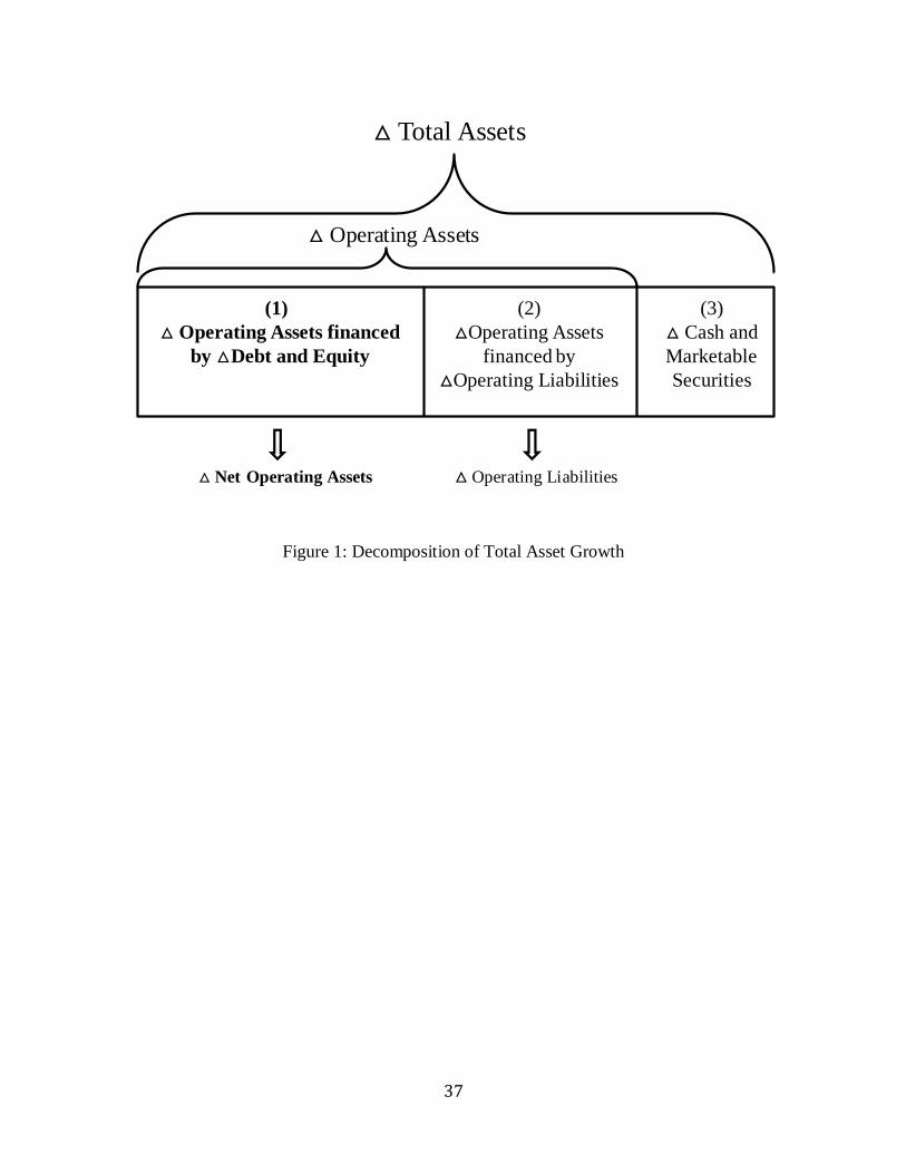
[Insert Figure 1]

Decomposition of TA Growth

Total assets can be decomposed as:

TA OA CASH (1)

11

Where TA, OA and CASH represent Total Assets, Operating Assets, and Cash

and Marketable Securities, respectively.

Consistent with related literature (Hirshleifer et al. 2004; Richardson et al. 2005;

Fairfield et al. 2003), operating assets can be further divided into operating assets

financed by operating liabilities (OAOL) and operating assets financed by debt and equity

(i.e., NOA).

Adding and subtracting OAOL from equation (1), I get

( ) (2)OL OL OLTA OA OA OA CASH NOA OA CASH

NOA is the part of operating assets financed by debt and equity. When suppliers

allow sales on account, an increase in operating assets will be accompanied by an

increase in operating liabilities. Hence, OAOL is equal to the amount of operating

liabilities.

Taking first difference of equation (2) between year t and year t-1, I have

OLTA NOA OA CASH (3)

Therefore, TA growth decomposes into NOA growth, growth in OAOL and

growth in CASH.

12

III. DATA AND RESULTS

Consistent with Cooper et al. (2008), I use all NYSE, AMEX and NASDAQ non-

financial firms (i.e., excluding firms with four-digit SIC codes between 6000 and 6999)

listed on the CRSP monthly stock returns files and the Compustat annual industrial files.

My sample spans the period from 1968 to 2008. In addition, I restrict the sample to firms

with year-end price greater than $5.6 This requirement eliminates very small firms,

which have been shown to have high transaction cost and illiquidity, making trading

strategies unrealizable (Fama 1998; Fama and French 2008). After I eliminated firm-

years without adequate data to compute any financial statement variables or returns, the

sample contains 99,194 firm-years.

Definition of Variables

The main variable of concern, the annual firm asset growth rate (TAgrowth) is

calculated using the year-on-year percentage change in total assets (Compustat item

numbers are included in parentheses). Following Cooper et al. (2008), a firm must have

non-zero and non-missing total assets in both year t and t-1 to compute this measure

1

1

( 6) ( 6)

( 6)

t tt

t

TA Data TA DataTAgrowth

TA Data

(4)

Net operating asset (NOA) growth is calculated as the difference between

operating asset growth and operating liability growth, scaled by lagged total asset, as

6 The sample used Cooper et al. (2008) is from 1968 to 2003. The results in this study are robust to Cooper

et al.’s (2008) sample period and non-elimination of the very small firms.

13

1 1

1

( ) ( )

( 6)

t t t tt

t

OA OA OL OLNOAgrowth

TA Data

(5)

Consistent with Cooper et al. (2008) and Hirshleifer et al. (2004), 7

operating

assets are calculated as the residual of total assets after subtracting cash and marketable

securities, as follows;

( 6) ( 1)t t tOA TA Data CASH Data (6)

Operating liabilities are the residual amount from total assets after subtracting

financial liabilities and equity.

t t t t

t t

t

OL TA ( Data6 ) Short-term Debt ( Data34 ) Long-term Debt ( Data9 )

Minority Interest ( Data38 ) Preferred Stock (Data130)

Common Equity ( Data60 )

(7)

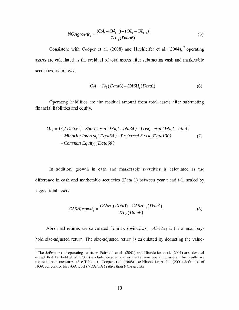
In addition, growth in cash and marketable securities is calculated as the

difference in cash and marketable securities (Data 1) between year t and t-1, scaled by

lagged total assets:

1

1

( 1) ( 1)

( 6)

t tt

t

CASH Data CASH DataCASHgrowth

TA Data

(8)

Abnormal returns are calculated from two windows. Abrett+1 is the annual buy-

hold size-adjusted return. The size-adjusted return is calculated by deducting the value-

7 The definitions of operating assets in Fairfield et al. (2003) and Hirshleifer et al. (2004) are identical

except that Fairfield et al. (2003) exclude long-term investments from operating assets. The results are

robust to both measures. (See Table 4). Cooper et al. (2008) use Hirshleifer et al.’s (2004) definition of

NOA but control for NOA level (NOAt/TAt) rather than NOA growth.

14

weighted average return for all firms in the same market-capitalization-matched decile.

The return accumulation period covers twelve-months, beginning four months after the

end of the fiscal year, to ensure complete dissemination of accounting information in

financial statements of the previous year. Similar to Sloan (1996) and Cheng et al. (2006),

Ret3t+1 is announcement returns calculated as the twelve-day size-adjusted return,

consisting of the four three-day (-1,0,1) periods surrounding quarterly earnings

announcements in year t+1.

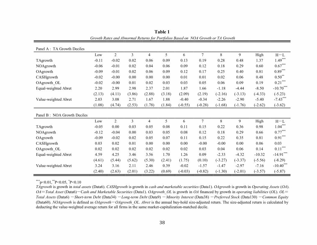
[Insert Table 1]

Table 1 reports the abnormal returns of both NOA growth and TA growth

strategies. The t-statistics are thus computed over 41 observations, corresponding to the

years 1968 to 2008. The lowest decile of TA growth earns an EW (VW) abnormal return

of 2.2 (2.03) percent, while the top decile earns an average EW (VW) abnormal return of

-8.5 (-5.4) percent. In contrast, firms in the bottom decile of NOA growth earn an EW

(VW) abnormal return of 4.59 (3.24) percent and those in the top decile earn an EW

(VW) abnormal return of -10.32 (-7.16) percent. These results are similar to those

reported by Cooper et al. (2008), Fairfield et al. (2003) and Richardson et al. (2005).

Besides the successful replication of the TA and NOA growth anomalies, it is interesting

to note that the average hedge returns of the NOA growth strategy are 40 percent greater

(with greater t-statistics, as well) than those of the TA growth strategy in both equal-

weighted and value-weighted portfolios. In other words, the two additional components

15

dilute the abnormal negative returns of the NOA growth strategy by 28 (29.7) percent and

reduce the t-statistics by 36 (38) percent for EW (VW) portfolios.

Table 1 also reports the time-series average of yearly cross-sectional median of

growth rates. Panel A shows that, moving from the bottom decile of TA growth to the

top decile, the TA growth rate increases by 1.49,the NOA growth rate increases by

0.67,the cash growth rate increases by 0.5 and the operating liability growth rate

increases by 0.21. Panel B suggests that, from the bottom decile of NOA growth to the

top decile, the TA growth rate increases by 1.04, the NOA growth rate increases by 0.77,

the cash growth rate increases by 0.03 (statistically insignificant) and operating liability

growth rate increases by 0.11.

Sorting on TA growth leads to a higher top-to-bottom spread in cash growth rate

and operating liability growth rate than sorting on NOA growth. This finding suggests

that, in the top (bottom) decile of TA growth, high (low) TA growth is driven by either

high (low) NOA growth or high (low) growth in cash and operating liabilities. In addition,

the decile of TA growth have a lower top-to-bottom spread in NOA growth rate, and the

decile of NOA growth have a lower top-to-bottom spread in TA growth.

If TA growth is the primary driver of future returns, the magnitude of hedge

returns should mirror the magnitude of the top-to-bottom spread in TA growth. However,

the fact that the magnitude of hedge returns mirrors the spread in NOA growth rather

than TA growth suggests that NOA growth may be the major forecasting variable of

future negative returns.

16

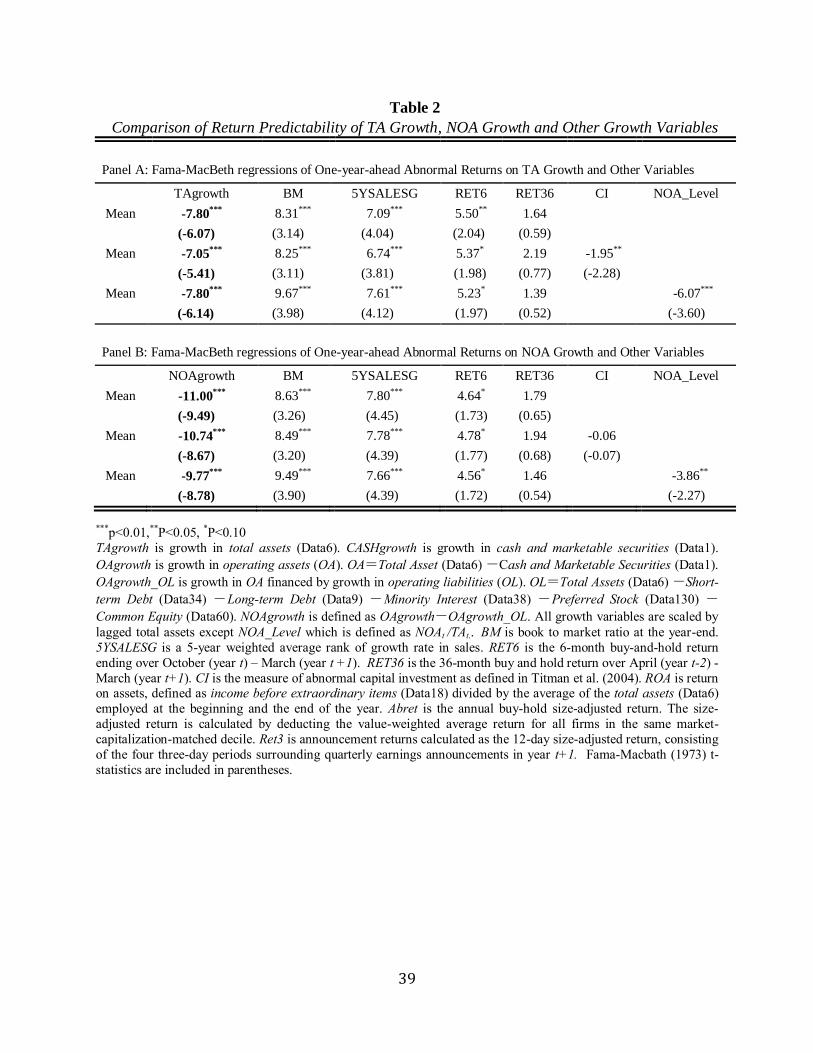
[Insert Table 2]

In Panel A of Table 2, I test the robustness of TA growth to a set of control

variables that include the book-to-market ratio, six-month lagged returns, 36-month

lagged returns, abnormal capital investment and sales growth rates (Debont and Thaler

1985; Fama and French 1992; Jagadeesh et al. 1993; Titman et al. 2004; Lakonishok et al.

1994). I perform Fama and MacBeth (1973) cross-sectional regression of one-year ahead

abnormal returns on TA growth and the other firm characteristics for forty-one years in

the sample. Following standard practice, all return forecasting variables are ranked

annually by deciles and are scaled to take a value between -0.5 and 0.5. Thus, the

coefficients on forecasting variables can be interpreted as the incremental abnormal

returns of a zero-investment strategy in the respective variables. Tests of statistical

significance of the coefficients are based on the standard errors calculated from the

distribution of individual yearly coefficients. This test overcomes bias due to cross-

sectional dependence in error terms (Bernard 1987).

The results are similar to those of Cooper et al. (2008), and not surprisingly, most

of coefficients on the control variables are significant. The TA growth is not subsumed

by the other important determinants of the cross-section. In fact, the TA growth’s t-

statistics range from -5.4 to -6.14, appearing to be the strongest determinant relative to all

other determinants. This result confirms the strong negative and economically significant

relation between TA growth and one-year-ahead abnormal returns from the one-way sorts

of Table 1.

Panel B of Table 2 compares NOA growth with the same control variables. NOA

17

growth also appears to be robust to all of the other importance determinants of the cross-

sectional returns. More importantly, NOA growth has higher abnormal returns with

stronger t-statistics in each regression than TA growth, when comparing Panel A with

Panel B.

It is interesting to note that abnormal capital investment (Titman et al. 2004) is

robust to TA growth but is subsumed by NOA growth. Together with Table 1, these

results suggest that NOA growth alone has stronger predictability in future abnormal

returns than TA growth.

Cooper et al. (2008) attempt to control the level of NOA, rather than NOA growth,

in their analysis. The NOA level (NOAt/ATt) is defined as NOAt scaled by total assets of

the current year. 8 Regression 3 of Panel A in Table 2 shows that the TA growth anomaly

is robust to the NOA level, consistent with the results of Cooper et al. (2008). If NOAt-1

is the market expectation of NOAt at announcement dates, NOA growth (NOAt- NOAt-1)

can be viewed as a proxy for an unexpected NOA component of NOAt.9

Papanastasopoulos et al. (2010) suggest that an unexpected NOA component actually

drives future negative returns. Therefore, NOA growth, as new information that has not

been priced, is more likely associated with unexpected returns than the NOA level.

Comparing the TA Growth Anomaly with the NOA Growth Anomaly

So far, the NOA growth strategy and the TA growth anomaly have been examined

8 The NOA level (NOAt/ATt) is different from Hirshleifer et al. (2004)’s NOAt/ATt-1. Hirshleifer et al.

(2004)’s NOAt/AT t-1 can be considered as a NOA growth measure when NOAt/AT t-1 is decomposed into

9 Bernard and Thomas (1989) define unexpected earnings components in a similar way.

1 1 1 1

1 1 1 1 1

1t t t t t tt

t t t t t

NOA NOA NOA NOA OL CashNOAgrowth

AT AT AT AT AT

18

independently. In the following analyses, I investigate whether the NOA growth anomaly

subsumes the TA growth anomaly. I will sequentially report results from two-way

portfolio analyses, regression analyses, shorter-window return analyses, and non-overlap

hedge analyses.

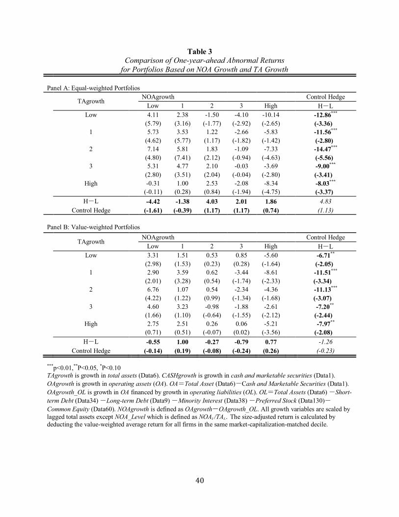
[Insert Table 3]

In Table 2, the regression approach gives advantages in multivariate analyses and

simplifies the interpretation of results. As discussed in Section II, the studies comparing

two anomalies employ a common approach complementary to a cross-sectional

regression, running a cell-based portfolio analysis on abnormal returns of interest

variables. To implement the two-way sorting analyses, I sort stocks independently on TA

and NOA growth at a time and then focus on the intersections resulting from these

independent sorts. This procedure assigns the stocks to twenty-five cells, as shown in

Table 3. This table contains the EW (VW) size-adjusted returns of NOA growth-TA

growth portfolio combinations. By reading across the rows in Table 3, one can observe

abnormal returns to NOA growth portfolios, holding TA growth constant. Similarly, in

each column, one can assess the abnormal returns to the TA strategy holding NOA

growth constant. Similar to the returns reported in Table 1, the returns and the

corresponding t-statistics are based on a time-series of 41 annual observations.

Recall that Table 1 shows that basic NOA growth and TA growth hedges earn

EW (VW) abnormal returns of -14.91(-10.40) percent and -10.7(-7.42) percent,

respectively. It is also important to note that the hedge returns are not necessarily the

19

difference between the lowest quintile and the highest quintile in this control-hedge

setting. Because of the positive correlation between NOA and TA growth shown in Table

1, the independent two-way sorting results in no observations in some intersections of

extreme quintiles (e.g., lowest (highest) TA growth and highest (lowest) NOA growth

quintiles) in some years. Therefore, in these years, the hedge returns are calculated from

the intersections of the second lowest (highest) quintile. When Desai et al. (2004)

compare the accrual anomaly with the value-glamour anomaly, the same case appears in

their Table 5 and Table 6. Under the two-way sorting portfolio tests reported in Table 3,

the NOA growth strategy still earns large negative abnormal returns ranging from -8

percent to -13 percent across TA growth rows, while the TA growth strategy does not

survive in any of NOA growth columns. Therefore, in two-way sorting portfolio analyses,

Cooper et al.’s (2008)’s TA growth anomaly is completely subsumed by the NOA growth

anomaly.

The Predictability of the Additional Two Subcomponents in Future Abnormal

Returns

Table 3 has shown that the TA growth anomaly is subsumed by the NOA growth

anomaly. Table 4 shows the incremental predictability of the TA growth’s two additional

components (i.e., growth in CASH and OAOL) for future negative returns over NOA

growth. The Fama-Macbeth (1973) regression approach involves projecting size-

adjusted abnormal returns on different growth components (i.e., growth in CASH, OAOL,

TA and NOA). All growth components are ranked annually by deciles and are scaled to

20

take a value between -0.5 and 0.5. Thus, the coefficients on growth components can be

interpreted as the abnormal return to a zero-investment strategy in the respective variable.

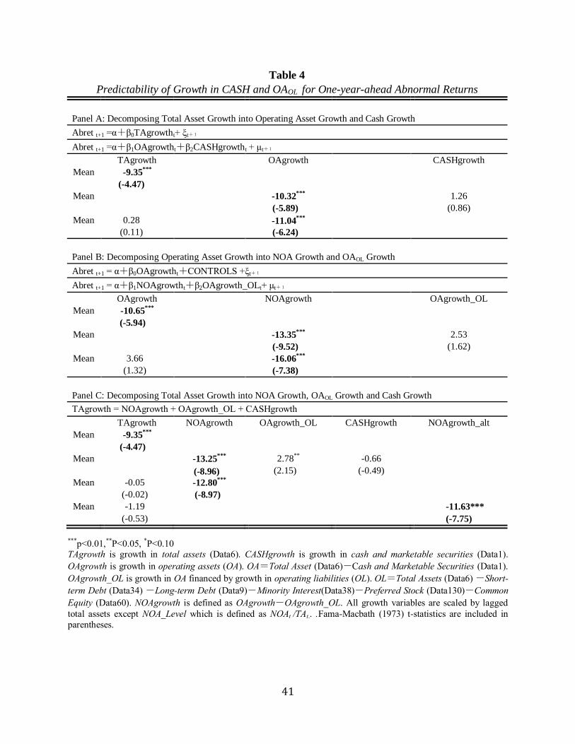
[Insert Table 4]

The regression analysis in Panel A of Table 4 confirms the results (in Panel A of

Table 1) that TA growth alone can predict significant negative future returns (t-statistic=

-4.47). When TA growth is decomposed into growth in operating assets and CASH

growth (regression two in Panel A of Table 4), CASH growth has no incremental return

predictability over growth in operating assets (t-statistic= 0.86) when controlling growth

in operating assets. Therefore, when operating asset growth and TA growth are

considered together in the regression (regression three in Panel A of table 4), the

incremental return to TA growth become insignificant (t-statistics= 0.11) while the

incremental returns to an operating asset strategy are large (-11.04 percent) and

significant (t-statistics=-6.24). It suggests that the TA growth strategy is likely subsumed

by the operating asset growth strategy because CASH growth has no incremental return

predictability.

In Panel B of Table 4, operating assets are decomposed into NOA and OAOL. I

show that OAOL growth is a redundant component of operating asset growth in predicting

future negative returns (t-statistic= 1.62). When operating asset growth and NOA growth

are considered together in the regression, the incremental return to operating asset growth

becomes insignificant (t-statistics=1.32) while the incremental returns to an NOA

strategy continue to be large (-16.06 percent) and significant (t-statistics=-7.38). It

21

suggests that the abnormal returns associated with operating assets growth are likely

attributable to NOA growth because growth in OAOL is a redundant component of

operating assets.

Panel C of Table 4 combines the evidence of Panel A and Panel B and shows that

growth in CASH and OAOL, as the two additional components of TA growth, has no

predictability in future negative returns incremental to NOA growth. Therefore, when

TA growth and NOA growth are considered together in the regression, the incremental

returns to TA growth become insignificant (t-statistics=-0.02) while the incremental

return to NOA strategy continues to be large (-12.80 percent) and significant (t-statistic=-

8.97).10

Consistent with the two-way sorting analyses, the regression analyses confirm

that the TA growth anomaly is attributable to the NOA growth anomaly. In addition, the

third regression in Panel C of Table 4 shows that the result is robust when using an

alternative NOA growth measure.11

The Implications of TA growth’s subcomponents for Future Profitability

Table 4 examines the return predictability of the TA growth’s three subcomponents.

Table 5 shows the implications of TA growth and its three subcomponents for one-year-

ahead ROA, and Table 6 tests whether the abnormal negative returns associated with

growth components are attributable to the market’s misunderstanding of these

implications for future ROA. Following Fairfield et al. (2003), future profitability is

defined as one-year-ahead Return on Assets (ROA). ROA is defined as income before

10 The result is robust when adding the set of comparing variables in Table 2. 11 Discussed in the data definition section.

22

extraordinary items divided by the average of the total assets employed at the beginning

and the end of the year. Each regression in Table 5 includes lagged ROA (Fairfield et al.

2003) and lagged ROA change (Cao et al. 2010) as previously suggested control

variables for future ROA.12

All growth components are ranked annually by deciles and

are scaled to take a value between -0.5 and 0.5.

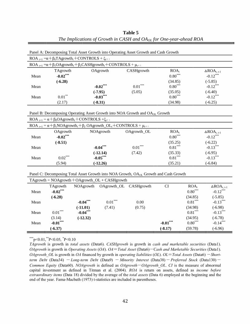
[Insert Table 5]

In Panel C of Table 5, TA growth alone has significant negative effects on future

ROA (t-statistic=-6.28) after controlling previously suggested determinants of one-year-

ahead ROA. TA growth is decomposed into growth in NOA, OAOL and CASH in

regression two of Panel C of Table 5. Consistent with prior literature (e.g., Fairfield et al.

2003; Richardson et al. 2005), NOA growth has strong negative implications on future

profitability (t-statistic =-11.01) while growth in CASH (t-statistic=0.75) and OAOL (t-

statistic=7.41) do not have negative effects on one-year-ahead ROA. Therefore, when

NOA growth and TA growth are considered together in the regression (regression three

in Panel C of Table 5), the negative effect of TA growth on future ROA becomes non-

negative (t-statistic= 3.14) while the incremental effect of NOA growth on future ROA

remains significantly negative (t-statistic=-12.32). It suggests that the negative effect of

TA growth on future ROA is driven by only one of TA’s subcomponents - NOA growth.

The two additional components (i.e., growth in CASH and OAOL) do not contribute to the

negative implication of TA growth for one-year-ahead ROA.

12 Results are very similar when dropping lagged ROA change.

23

Comparing Table 4 with Table 5, one can see that the abnormal negative returns

mirror the negative implications for future ROA. The components with negative

implications (i.e., growth in NOA, operating assets and TA) generate negative future

returns while components (i.e., growth in CASH and OAOL) with statistically

insignificant or positive implications do not predict future negative returns. Moreover, the

fact that the negative implications of TA growth are subsumed by NOA growth mirrors

the result that the predictability of TA growth in future returns is subsumed by NOA

growth. All of the evidence is consistent with Fairfield et al. ’s (2003) argument that the

abnormal negative returns are due to the market’s failure to incorporate the negative

implications of growth for future ROA in a timely fashion. The negative returns in

subsequent periods were realized when the market gradually responds to the negative

implications. This explanation is further corroborated by the fact that the negative

implication of TA growth for future ROA is robust to abnormal capital investment (Table

5) mirroring the finding that the predictability of TA growth in future returns is robust to

abnormal capital investment shown (Table 2).

Market Understanding of the Implications of TA’s subcomponents for Future ROA

Following Fairfield et al. (2003) and Collin and Hribar (2000), this subsection

shows that the market underreacts to the negative implications of growth components for

future ROA through the Mishkin (1983) test. Mishkin (1983) develops a framework to

test whether investors price publicly available information rationally. In the Mishkin Test,

two equations (i.e., a forecasting equation and a valuation equation) are simultaneously

24

estimated. Coefficients in the forecasting equation (i.e., forecasting coefficients) are the

actual effects of growth components on one-year-ahead ROA, similar to the analyses in

Table 5. The coefficients in the valuation equation (i.e., valuation coefficients) are

inferred from the market’s pricing of the actual effect, and they represent the market’s

assessment of the actual effects. The Mishkin test provides a statistical comparison

between with the actual effect for future ROA (i.e., forecasting coefficients) and the

market’s assessment of the effect (i.e., valuation coefficients). If the actual effect of a

growth component is equal to the market’s assessment, then the market is efficient in

pricing the effect of the growth component on future ROA. Otherwise, the market fails

to incorporate the actual effect of the growth component on future ROA into price in a

timely fashion. Abnormal returns are subsequently earned when the market gradually

learns about the true effect.

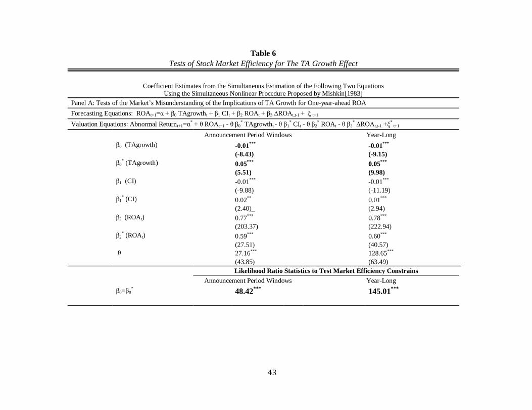
[Insert Table 6]

In Panel A of Table 6, the forecasting equation is similar to regression 4 of Table

5 Panel C. The coefficients β0 and β1 are the actual effects of TA growth and abnormal

capital investment on future ROA, respectively. Consistent with the results in Table 5, the

implications of TA growth for future ROA remains significantly negative (β0=-0.01) after

controlling for abnormal capital investment. As discussed earlier, the valuation

coefficient β0* (=0.05) reflects the market assessment of TA growth’s actual effect on

future ROA (i.e., β0). The restriction β0= β0* yields a likelihood ratio statistic, which has a

25

chi-square distribution. The likelihood ratio statistic for the restriction β0= β0* is highly

significant for both announcement and year-long windows, indicating that the market

fails to incorporate the negative implications of TA growth for future ROA. The market

perceives TA growth as a good signal for future ROA while TA growth actually has

negative implications. Abnormal negative returns are subsequently earned when the

market gradually learns about the negative effect of TA growth.

The market also perceives an increase in capital investment as a positive signal

for future ROA (β1*=0.01) while this increase has negative implications for future

profitability (β1=-0.01). This result corroborates Titman et al.’s (2004) explanation that

the abnormal negative returns of abnormal capital investment is due to the market’s

misunderstanding of the empire-building implications associated with abnormal capital

investment. .

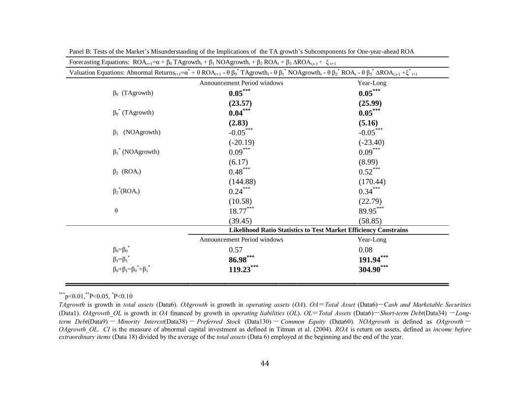
Panel B of Table 6 shows that, out of the three components of TA growth, stock

prices fail to reflect the negative implications of NOA growth but correctly price the non-

negative implications of growth in CASH and OAOL. β0 is the incremental effect of TA

growth for future ROA over NOA growth; thus, it represents the actual average effect of

the additional two components (i.e., growth in CASH and OAOL) on one-year-ahead

ROA. The market assessment β0* (=0.04) is close to the actual effect β0 (=0.05). The

likelihood ratio statistic for the restriction β0= β0* is not significant, indicating that the

market correctly prices the non-negative implications of these two components. This

result is consistent with Panel A and prior studies (McConnell and Muscarella 1985;

Blose and Shieh 1997; Vogt 1997), which show that the market, on average, perceives

asset growth (e.g., growth in TA, NOA, CASH, OAOL and capital investment) as a good

26

signal for future profitability. Therefore, the market is more likely to respond correctly to

the growth components that have non-negative implications (e.g., growth in CASH and

OAOL) as opposed to negative-implication components. As a result, the two additional

components fail to predict future negative returns and are noisy components of TA

growth. On the other hand, the likelihood ratio statistics on β1= β1* and β0 +β1= β0

* +β1

*

are highly significant, showing that the market fails to incorporate the negative

implications of NOA growth. Hence, the abnormal negative returns of the TA growth

anomaly are driven by the market’s misunderstanding of the negative implications

associated with one of TA growth’s subcomponents (i.e., NOA growth).

The use of the Mishkin test is not without controversy. Kothari, Sabino and Zach

(2005) argue that the test results are sensitive to survivorship biases and truncation errors.

More recently, Kraft, Leone and Wasley (2007) argue that the test is not superior to OLS.

I remain agnostic about the merits of the Mishkin test and report both the Fama-Macbeth

OLS results and the Mishkin test results in Tables 5 and 6, respectively.

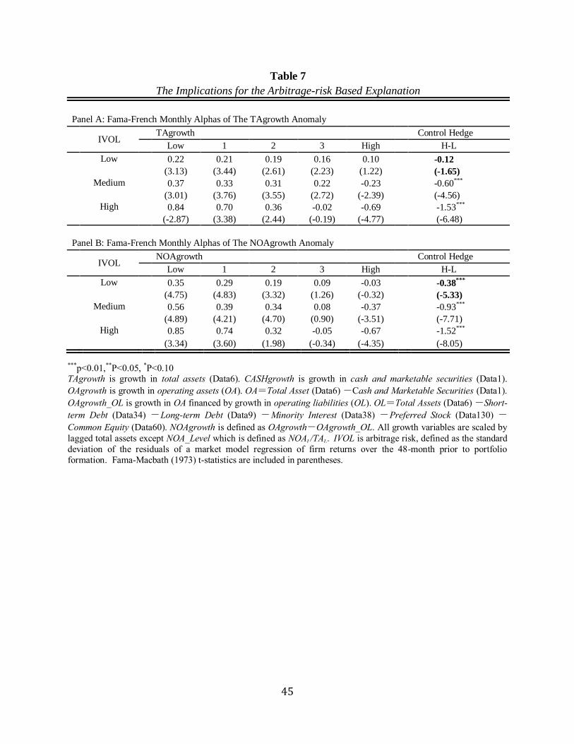
[Insert Table 7]

The implications For the Arbitrage-Based Explanation

Lam and Wei (2010) and Lipson et al. (2009) use TA growth as the ―growth

effect‖ measure and document that the abnormal returns following TA growth are not

robust to arbitrage risk. They argue that the ―growth effect‖ can be explained by arbitrage

risk. I demonstrate the economic significance of using the correct growth anomaly proxy

27

by showing the differential robustness of TA growth and NOA growth to arbitrage risk In

Table 7. Arbitrage risk (IVOL) is defined as the standard deviation of the residuals of a

market model regression13

of firm returns over the 48-month prior to portfolio formation.

Panel A of Table 7 shows the robustness of the TA growth anomaly to arbitrage risk.

Similar to Lam and Wei (2010) and Lipson et al. (2009), I find that the TA growth

anomaly generates no abnormal returns in the lowest arbitrage risk portfolio. However,

Panel B of Table 7 shows that the NOA growth strategy still leads to statistically

significant negative returns when arbitrage risk is absent/low. This result demonstrates

that using the correct growth anomaly measure leads to a different result.

Tests of Risk-Based Explanations

Table 8 and Table 9 demonstrate that the superior predictive power of NOA

growth over TA growth in returns is not due to NOA growth being more exposed to risk

factors. Cheng et al. (2006) show that while the value-glamour (CFO/P) anomaly

subsumes the accrual anomaly in annual windows (Desai et al 2004), the two anomalies

present different abnormal returns patterns over shorter windows around earnings

announcements. In short windows, missing risk factors are of less concern relative to

annual windows (Brown and Warner 1980; 1985; Kothari 2001). Cheng et al. (2006)

conclude that the two anomalies may differ from each other. In Table 8, I confirm the

annual window result that the NOA growth anomaly completely subsumes the TA growth

anomaly in Table 3 and Table 4 using returns around earnings announcements. The TA

13 I follow Lam and Wei (2010) and Lipson et al. (2009) using the S&P 500 index to proxy the market

index. The results are similar when the proxy is the CRSP equal-weighed or value-weighted market

portfolio.

28

growth strategy alone generates significant negative returns (t-statistic=-3.56) around

subsequent earnings announcements. However, when TA growth and NOA growth are

considered together in the regression, the incremental short-window returns to TA growth

become insignificant (t-statistics=0.32) while the incremental short-window return to

NOA strategy continues to be large (-1.9 percent) and significant (t-statistic=-5.78). It

suggests that missing risk factors are not likely to explain the superior predictability of

NOA growth over TA growth.

Recall that abnormal capital investment (Titman et al. 2004) is robust to TA

growth but is subsumed by NOA growth in the annual windows of Table 2. Table 9

confirms this result on shorter windows around earnings announcements, indicating that

NOA growth is a stronger growth anomaly measure that TA growth.

[Insert Table 8]

This study is the first to investigate the NOA growth strategy in short-window

periods. Because there is less concerns regarding missing risk factors in short-windows

relative to annual windows, the strong abnormal returns of NOA growth documented in

Table 9 extend Fairfield et al.’s (2008) finding on annual windows and corroborate the

mispricing explanation for NOA growth.

[Insert Table 9]

29

Table 9 examines whether NOA growth is more exposed to existing risk factors

(e.g., beta, SML, HML and MOM) than TA growth. Panel A shows the average monthly

raw returns from equal-weighted portfolios as a reference benchmark for the following

panels. Panels B, C, D show the CAPM monthly alphas, Fama-French monthly alphas

and Carhart four-factor14

monthly alphas, respectively. Panel B shows that, under two-

way sorting portfolio tests, the NOA growth strategy generates large negative returns

while the TA growth strategy returns remain insignificant after controlling beta. It

suggests that NOA growth is not more exposed to beta, relative to TA growth. Panel B

also suggests that the long-short NOA growth strategy is beta-insensitive in that beta does

not change the hedge returns of the NOA growth strategy but only reduces portfolio

returns in each of twenty-five cells. Panel C and Panel D suggest similar patterns,15

except that Panel D shows that the returns from NOA growth strategy are, to some degree,

associated with Carhart’s (1997) momentum factor. Collectively, the results show that

the superior predictive power of NOA growth over TA growth in returns is not due to

NOA growth being more exposed to risk factors.

Robust Tests Using Non-Overlap Hedge Analyses

In Table 10, I employ the nonoverlap hedge test suggested by Desai et al. (2004)

as a robust test. The nonoverlap hedge strategy eliminates firms in convergent extreme

groups and leaves nonoverlap observations in the top and bottom deciles. I form a new

portfolio (labeled as "nonoverlap hedge") where I eliminate firm-years in these

14 Obtained from Ken French’s web page 15 Panel D and Panel E show that the hedge returns of TA growth strategies not only remain insignificant

but also become even positive in some columns after controlling the risk factors and NOA growth.

30

convergent cells and assess whether each of the strategies can individually generate

abnormal returns. In other words, I decompose firms in the top (bottom) decile of TA

growth firms into two groups: a group where high (low) TA growth is driven by high

(low) NOA growth and a group where high (low) TA growth is driven by high (low)

growth in CASH and OAOL.

[Insert Table 10]

Table 10 shows that only the observations for which high (low) TA growth is

driven by high (low) NOA growth explain the TA growth anomaly shown by Cooper et

al. (2008). The observations where high (low) TA growth is driven by high (low) growth

in CASH and OAOL fail to predict future returns (t-statistic=-0.82) and, in fact, dilute the

predictability of NOA growth. Analogously, I form a nonoverlap hedge portfolio for

NOA growth by taking a long position on the highest NOA growth after eliminating the

highest TA growth firms and a short position on the lowest NOA growth after eliminating

the lowest TA growth firms. The non-overlap hedge return from NOA growth after

eliminating extreme TA growth firms continues to generate large abnormal returns (-

14.08 percent). Therefore, the results from non-overlap hedges confirm the findings in

Table 3 and Table 4 that NOA growth is the only driver for TA growth’s future negative

returns. In summary, the newly influential TA growth anomaly found in the finance

literature appears to be a noisy manifestation of the NOA growth anomaly documented in

earlier accounting literature.

31

IV. CONCLUSIONS

Cooper et al. (2008) is a recent influential study on market efficiency. They show

that firms with high TA growth tend to have substantial negative abnormal returns in

subsequent periods. However, the source of the TA growth’s abnormal returns has

remained a puzzle. In this study, I show that the TA growth anomaly is totally subsumed

by the NOA growth anomaly. The results are robust to short- and long- window returns,

value-weighted and equal-weighted portfolios and a battery of risk factors.

I decompose TA growth into NOA growth and two additional components (i.e.,

growth in CASH and OAOL) and show that the market, on average, perceives growth in

any asset component as a good signal for future profitability. The abnormal negative

returns of TA growth are, thus, attributable to the market’s misunderstanding of the NOA

growth’s negative implications for future profitability. The two additional components

do not have negative implications for future profitability and, on average, are correctly

priced by the market. Therefore, the two additional components do not have predicative

power for future negative returns beyond NOA growth. They rather dilute the

predictability of NOA growth by reducing abnormal returns and t-statistics by 28 percent

and 36 percent. The superior predictability power of NOA growth in relation to TA

growth leads these two anomalies to have differential robustness to market-friction

controls. It demonstrates the economic significance of using the correct anomaly measure.

Cooper et al. (2008) inspired several studies (e.g., Chen, Yao and Yu 2010; Gray

and Johnson 2010) that examine whether the TA growth anomaly exists in global

32

financial markets. Additionally, they seek to identify cross-country interactive effects for

TA growth’s abnormal returns. These studies consider TA growth to be the best growth

measure and generalize their findings to a ―growth effect.‖ Because TA growth carries

two noisy components, the abnormal returns of TA growth will likely interact with noisy

cross-country variables. In light of the evidence presented regarding the differential

robustness to arbitrage risk between TA and NOA growth, it would be interesting to

investigate whether all the results regarding TA growth anomalies remain robust when

TA growth is replaced by NOA growth.

This study has important implications for the underlying reasons behind the

―growth effect.‖ The results here suggest that not all growth components contribute to the

―growth effect‖ (i.e., growth in CASH and OAOL). The types of assets that are growing

and the finance sources of asset growth need to receive greater attention in future studies.

REFERENCES

Asquith, P. 1983. Merger bids, uncertainty, and stockholder returns. Journal of Financial

Economics 11 (April): 51-83.

Banz, R. 1981. The relationship between return and market value of common stocks.

Journal of Financial Economics 9: 3-18.

Bernard, V. 1987. Cross-sectional dependence and problems in inference in market-based

accounting research. Journal of Accounting Research 25(1): 1-48.

, and J. Thomas. 1989. Post-earnings announcement drift: delayed price response

or risk premium. Journal of Accounting Research 27: 1-36.

, and . 1990. Evidence that stock prices do not fully reflect the implications

of current earnings for future earnings. Journal of Accounting and Economics

13(4): 305-340

33

Blose, L. E., and J. C. P. Shieh. 1997. Tobin’s q-ratio and market reaction to capital

investment announcements. Financial Review 32: 449-476

Biais, B., and C. Gollier. 1997. Trade credit and credit rationing. The Review of Financial

Studies 10(4): 903 -937

Brown, S., and J. Warner. 1980. Measuring security price performance. Journal of

financial Economics 8: 205-258.

, S., and J. Warner. 1985. Using daily stock returns: the case of event studies.

Journal of Financial Economics 14(1): 3-31.

Cao, Y., L. A. Myers, and T. Sougiannis. 2010. Does earnings acceleration convey

information? The Review of Accounting Studies. Forthcoming.

Chen, L., and L. Zhang. 2010. A better three-factor model that explains more anomalies.

The Journal of Finance 65(2): 563-595.

Cheng, C., and W. Thomas. 2006. Evidence of the abnormal accrual anomaly incremental

to operating cash flows. The Accounting Review 81(5): 1151-1167.

Chordia, T., and S. Lakshmanan, 2006. Earnings and price momentum. Journal of

Financial Economics 80:627-656

Collins, D., and P. Hribar. 2002. Earnings-based and accrual-based market anomalies:

one effect or two. Journal of Accounting and Economics 29: 101-123.

Cooper, M., H. Gulen, and M. Schill. 2008. Asset growth and the cross-section of stock

returns. The Journal of Finance 63(4): 1609–1651.

Daniel, C., and T. Lys. 2006. Weighing the evidence on the relation between external

corporate financing activities, accruals and stock returns. Journal of Accounting

and Economics 42(1-2): 87-105.

DeBondt, W., and R. Thaler, 1985. Does the market overreact? Journal of Finance 40:

793–805.

Desai, H., S. Rajgopal, and M. Venkatachalam. 2004. Value glamour and accrual

mispricing. One anomaly or two. The Accounting Review 79(2): 355-385.

Fairfield P., S.Whisenant and T. Yohn. 2003. Accrued earnings and growth: implications

for future profitability and market mispricing. The Accounting Review 78(1): 353-

371.

Fama, E., and J. MacBeth. 1973. Risk, return, and equilibrium: empirical tests. The

Journal of Political Economy 81(30): 607-636.

34

, 1998. Market efficiency, long-term returns and behavioral finance. Journal of

Financial Economics 49: 283-306.

, and K. French. 1992. The cross-section of expected stock returns. The Journal of

Finance 47: 427-465.

, and . 2008. Dissecting anomalies. The Journal of Finance 64(4): 1653-1678.

Gray, P., and J. Johnson. 2010. The relationship between asset growth and the cross-

section of stock returns. Journal of Banking and Finance. forthcoming.

Greig, A. 1992. Fundamental analysis and subsequent stock returns. Journal of

Accounting and Economics 15(2/3): 413-442.

Harford, J. 1999. Corporate cash reserves and acquisitions. The Journal of Finance 54(6):

1969–1997.

Hirshleifer, D., K. Hou, S. Teoh, and Y. Zhang． 2004. Do investors overvalue firms

with bloated balance sheets. Journal of Accounting and Economics 38: 297-331.

Hong, H., T. Lim, and J. Stein. 2000. Bad news travels slowly: size, analyst coverage,

and the profitability of momentum strategies. Journal of Finance 55(1): 265-295.

Ibbotson, R. 1975. Price performance of common stock new issues. Journal of Financial

Economics 2: 235-272.

Jaffe, J., D. Keim, and R. Westerfield. 1989. Earnings yields, market values, and stock

returns. Journal of Finance 44(1): 135-148.

Jegadeesh, N., and S. Titman, 1993. Returns to buying winners and selling losers:

Implications for stock market efficiency. Journal of Finance 48: 65–91.

Jensen, M. 1986. The agency costs of free cash flow: corporate finance and takeovers.

American Economic Review, 76(2): 323-330.

Keynes, J. 1936. The General Theory of Employment, Interest and Money. Harcourt

Brace, London.

Kothari S. 2001. Capital markets research in accounting. Journal of Accounting and

Economics 31(1-3): 105-231.

, J. Sabino, and T. Zach. 2005. Implications of survival and data trimming for

tests of market efficiency. Journal of Accounting and Economics 39(1): 129-161.

Kraft, A., A. J. Leone, and C. E. Wasley. 2007. Regression-based tests of the market

pricing of accounting numbers: the mishkin test and ordinary least squares.

Journal of Accounting Research 45: 1–34.

35

Lakonishok, J., A. Shleifer, and R. Vishny. 1994. Contrarian investment, extrapolation,

and risk. Journal of Finance 49:1541–1578.

Lam, E., and J. Wei. 2010. The role of limits to arbitrage and the asset growth anomaly.

Available at: http://ssrn.com/abstract=1360680.

Lipson, M., S. Mortal, and M. Schill. 2009. What explains the asset growth effect in

stock Returns. Available at: http://ssrn.com/abstract=1364324.

Long, M., I. Malitz, and A. Ravid, 1994. Trade credit, quality guarantees, and product

marketability. Financial Management 22:117-127

Loughran, T., and J. Ritter. 1995. The new issues puzzle. Journal of Finance 50: 23-52.

Chan, K. L., J. Karceski, J. Lakonishok, and T. Sougiannis. 2008. Balance sheet growth

and the predictability of stock returns. Available at:

http://uic.edu/cba/Documents/Sougiannis-paper.pdf.

McConnell, J. J., and C. J. Muscarella. 1985. Corporate capital investment decisions and

the market value of the firms. Journal of Financial Economics 14:399-422

Mian, S. L., and C. W. Smith. 1994. Extending trade credit and financing receivables.

Journal of Applied Corporate Finance 7: 75-84

Mishkin, F. 1983. A Rational Expectations Approach to Macroeconomics: Testing Policy

Effectiveness on Efficient-Markets Models. Chicago, IL: University of Chicago

Press.

Opler, C., L. Pinkowitz, R. Stulz, and R. Williamson. 1999. The determinants and

implications of corporate cash holdings. Journal of Financial Economics 52: 3-

46.

Palazzo, B. 2009. Firms' cash holdings and the cross-section of equity returns. January 13.

Available at: http://ssrn.com/abstract=1339618.

Papanastasopoulos, G., D. Thomakos, and W. Tao. 2010. Information in balance sheets

for future stock returns: evidence from net operating assets. July 23. Available at:

http://ssrn.com/abstract=937361.

Reinganum, M. 1982. A direct test of roll’s conjecture on the firm size effect. Journal of

Finance 31: 27-35.

Richardson, S., R. Sloan, M. Soliman, and İ. Tuna. 2005. Accrual reliability, earnings

persistence and stock prices. Journal of Accounting and Economics 39(3): 437-

485.

, , , and . 2006. The implications of accounting distortions

and growth for accruals and profitability. The Accounting Review 81(3):713-743

36

Sloan, R. 1996. Do stock prices fully reflect information in accruals and cash flows about

future earnings?. The Accounting Review 71: 289-315.

Spiess, D., and J. Affleck-Graves. (1999). The long-run performance of stock returns

following debt offerings. Journal Financial Economics. 54: 45–73.

Stigler, G. 1963. Capital and Rates of Return in Manufacturing Industries. Princeton，

NJ: Princeton University Press.

Titman, S., K. Wei and F. Xie, 2004. Capital investments and stock returns. Journal of

Financial and Quantitative Analysis 39: 677-700.

Vogt, S. C. 1997. Cash flow and capital spending: evidence from capital expenditure

announcement. Financial Management 26:44-57

Yao, T., T. Yu, and T. Zhang. 2011. Asset growth and stock returns: evidence from Asian

financial markets. Pacific-Basin Finance Journal 19(1): 115-139.

37

Figure 1: Decomposition of Total Asset Growth

(1)

Operating Assets financed

by Debt and Equity

(2)

Operating Assets

financed by

Operating Liabilities

Net Operating Assets Operating Liabilities

Total Assets

Operating Assets

(3)

Cash and

Marketable

Securities

38

Table 1

Growth Rates and Abnormal Returns for Portfolios Based on NOA Growth or TA Growth

Panel A : TA Growth Deciles

Low 2 3 4 5 6 7 8 9 High H－L

TAgrowth -0.11 -0.02 0.02 0.06 0.09 0.13 0.19 0.28 0.48 1.37 1.49***

NOAgrowth -0.06 -0.01 0.02 0.04 0.06 0.09 0.12 0.18 0.29 0.60 0.67***

OAgrowth -0.09 -0.01 0.02 0.06 0.09 0.12 0.17 0.25 0.40 0.81 0.89***

CASHgrowth -0.02 -0.00 0.00 0.00 0.00 0.01 0.01 0.02 0.06 0.48 0.50**

OAgrowth_OL -0.02 -0.00 0.01 0.02 0.03 0.03 0.05 0.06 0.09 0.19 0.21***

Equal-weighted Abret 2.20 2.99 2.98 2.37 2.01 1.87 1.66 -1.18 -4.44 -8.50 -10.70***

(2.13) (4.11) (3.86) (2.88) (3.18) (2.09) (2.19) (-2.16) (-3.13) (-4.33) (-5.23)

Value-weighted Abret 2.03 3.08 2.71 1.67 1.88 -0.40 -0.34 -2.26 -2.90 -5.40 -7.43***

(1.08) (4.74) (2.53) (1.78) (1.84) (-0.55) (-0.28) (-1.68) (-1.76) (-2.62) (-3.62)

Panel B : NOA Growth Deciles

Low 2 3 4 5 6 7 8 9 High H－L

TAgrowth -0.05 0.00 0.03 0.05 0.08 0.11 0.15 0.22 0.36 0.98 1.04***

NOAgrowth -0.12 -0.04 0.00 0.03 0.05 0.08 0.12 0.18 0.29 0.66 0.77***

OAgrowth -0.09 -0.02 0.02 0.05 0.07 0.11 0.15 0.22 0.35 0.81 0.91***

CASHgrowth 0.03 0.02 0.01 0.00 0.00 0.00 -0.00 -0.00 0.00 0.06 0.03

OAgrowth_OL 0.02 0.02 0.02 0.02 0.02 0.02 0.03 0.04 0.06 0.14 0.11***

Equal-weighted Abret 4.59 4.25 3.46 3.56 1.70 1.26 0.09 -2.33 -4.32 -10.32 -14.91***

(4.61) (5.44) (5.62) (5.30) (2.41) (1.75) (0.10) (-3.27) (-3.37) (-5.56) (-8.29)

Value-weighted Abret 3.24 3.16 2.11 2.46 0.39 -0.02 -1.57 -1.47 -2.97 -7.16 -10.40***

(2.40) (2.63) (2.01) (3.22) (0.69) (-0.03) (-0.82) (-1.30) (-2.01) (-3.57) (-5.87)

***p<0.01,**P<0.05, *P<0.10 TAgrowth is growth in total assets (Data6). CASHgrowth is growth in cash and marketable securities (Data1). OAgrowth is growth in Operating Assets (OA).

OA＝Total Asset (Data6)－Cash and Marketable Securities (Data1). OAgrowth_OL is growth in OA financed by growth in operating liabilities (OL). OL＝

Total Assets (Data6) －Short-term Debt (Data34) －Long-term Debt (Data9) －Minority Interest (Data38) －Preferred Stock (Data130) －Common Equity

(Data60). NOAgrowth is defined as OAgrowth－OAgrowth_OL. Abret is the annual buy-hold size-adjusted return. The size-adjusted return is calculated by

deducting the value-weighted average return for all firms in the same market-capitalization-matched decile.

39

Table 2

Comparison of Return Predictability of TA Growth, NOA Growth and Other Growth Variables

Panel A: Fama-MacBeth regressions of One-year-ahead Abnormal Returns on TA Growth and Other Variables

TAgrowth BM 5YSALESG RET6 RET36 CI NOA_Level

Mean -7.80***

8.31*** 7.09*** 5.50** 1.64

(-6.07) (3.14) (4.04) (2.04) (0.59)

Mean -7.05

*** 8.25*** 6.74*** 5.37* 2.19 -1.95**

(-5.41) (3.11) (3.81) (1.98) (0.77) (-2.28)

Mean -7.80

*** 9.67*** 7.61*** 5.23* 1.39

-6.07***

(-6.14) (3.98) (4.12) (1.97) (0.52)

(-3.60)

Panel B: Fama-MacBeth regressions of One-year-ahead Abnormal Returns on NOA Growth and Other Variables

NOAgrowth BM 5YSALESG RET6 RET36 CI NOA_Level

Mean -11.00***

8.63*** 7.80*** 4.64* 1.79

(-9.49) (3.26) (4.45) (1.73) (0.65)

Mean -10.74

*** 8.49*** 7.78*** 4.78* 1.94 -0.06

(-8.67) (3.20) (4.39) (1.77) (0.68) (-0.07)

Mean -9.77

*** 9.49*** 7.66*** 4.56* 1.46

-3.86**

(-8.78) (3.90) (4.39) (1.72) (0.54)

(-2.27)

***p<0.01,**P<0.05, *P<0.10

TAgrowth is growth in total assets (Data6). CASHgrowth is growth in cash and marketable securities (Data1).

OAgrowth is growth in operating assets (OA). OA＝Total Asset (Data6) －Cash and Marketable Securities (Data1).

OAgrowth_OL is growth in OA financed by growth in operating liabilities (OL). OL＝Total Assets (Data6) －Short-

term Debt (Data34) －Long-term Debt (Data9) －Minority Interest (Data38) －Preferred Stock (Data130) －

Common Equity (Data60). NOAgrowth is defined as OAgrowth－OAgrowth_OL. All growth variables are scaled by

lagged total assets except NOA_Level which is defined as NOAt /TAt.. BM is book to market ratio at the year-end.

5YSALESG is a 5-year weighted average rank of growth rate in sales. RET6 is the 6-month buy-and-hold return

ending over October (year t) – March (year t +1). RET36 is the 36-month buy and hold return over April (year t-2) -

March (year t+1). CI is the measure of abnormal capital investment as defined in Titman et al. (2004). ROA is return on assets, defined as income before extraordinary items (Data18) divided by the average of the total assets (Data6)

employed at the beginning and the end of the year. Abret is the annual buy-hold size-adjusted return. The size-

adjusted return is calculated by deducting the value-weighted average return for all firms in the same market-

capitalization-matched decile. Ret3 is announcement returns calculated as the 12-day size-adjusted return, consisting

of the four three-day periods surrounding quarterly earnings announcements in year t+1. Fama-Macbath (1973) t-

statistics are included in parentheses.

40

Table 3

Comparison of One-year-ahead Abnormal Returns

for Portfolios Based on NOA Growth and TA Growth

Panel A: Equal-weighted Portfolios

TAgrowth

NOAgrowth Control Hedge

Low 1 2 3 High H－L

Low

4.11 2.38 -1.50 -4.10 -10.14

-12.86***

(5.79) (3.16) (-1.77) (-2.92) (-2.65)

(-3.36)

1

5.73 3.53 1.22 -2.66 -5.83

-11.56***

(4.62) (5.77) (1.17) (-1.82) (-1.42)

(-2.80)

2

7.14 5.81 1.83 -1.09 -7.33

-14.47***

(4.80) (7.41) (2.12) (-0.94) (-4.63)

(-5.56)

3

5.31 4.77 2.10 -0.03 -3.69

-9.00***

(2.80) (3.51) (2.04) (-0.04) (-2.80)

(-3.41)

High

-0.31 1.00 2.53 -2.08 -8.34

-8.03***

(-0.11) (0.28) (0.84) (-1.94) (-4.75) (-3.37)

H－L

-4.42 -1.38 4.03 2.01 1.86

4.83

Control Hedge (-1.61) (-0.39) (1.17) (1.17) (0.74) (1.13)

Panel B: Value-weighted Portfolios

TAgrowth

NOAgrowth Control Hedge

Low 1 2 3 High H－L

Low

3.31 1.51 0.53 0.85 -5.60

-6.71**

(2.98) (1.53) (0.23) (0.28) (-1.64)

(-2.05)

1

2.90 3.59 0.62 -3.44 -8.61

-11.51***

(2.01) (3.28) (0.54) (-1.74) (-2.33)

(-3.34)

2

6.76 1.07 0.54 -2.34 -4.36

-11.13***

(4.22) (1.22) (0.99) (-1.34) (-1.68)

(-3.07)

3

4.60 3.23 -0.98 -1.88 -2.61

-7.20**

(1.66) (1.10) (-0.64) (-1.55) (-2.12)

(-2.44)

High

2.75 2.51 0.26 0.06 -5.21

-7.97**

(0.71) (0.51) (-0.07) (0.02) (-3.56) (-2.08)

H－L

-0.55 1.00 -0.27 -0.79 0.77

-1.26

Control Hedge (-0.14) (0.19) (-0.08) (-0.24) (0.26) (-0.23)

***p<0.01,**P<0.05, *P<0.10

TAgrowth is growth in total assets (Data6). CASHgrowth is growth in cash and marketable securities (Data1).

OAgrowth is growth in operating assets (OA). OA＝Total Asset (Data6)－Cash and Marketable Securities (Data1).

OAgrowth_OL is growth in OA financed by growth in operating liabilities (OL). OL＝Total Assets (Data6) －Short-

term Debt (Data34) －Long-term Debt (Data9) －Minority Interest (Data38) －Preferred Stock (Data130)－

Common Equity (Data60). NOAgrowth is defined as OAgrowth－OAgrowth_OL. All growth variables are scaled by

lagged total assets except NOA_Level which is defined as NOAt /TAt.. The size-adjusted return is calculated by

deducting the value-weighted average return for all firms in the same market-capitalization-matched decile.

41

Table 4

Predictability of Growth in CASH and OAOL for One-year-ahead Abnormal Returns

Panel A: Decomposing Total Asset Growth into Operating Asset Growth and Cash Growth

Abret t+1 =α＋β0TAgrowtht+ ξt＋１

Abret t+1 =α＋β1OAgrowtht＋β2CASHgrowtht + μt＋１

TAgrowth

OAgrowth

CASHgrowth

Mean -9.35***

(-4.47)

Mean

-10.32

***

1.26

(-5.89)

(0.86)

Mean 0.28

-11.04***

(0.11)

(-6.24)

Panel B: Decomposing Operating Asset Growth into NOA Growth and OAOL Growth

Abret t+1 = α＋β0OAgrowtht＋CONTROLS +ξt＋１

Abret t+1 = α＋β1NOAgrowtht＋β2OAgrowth_OLt+ μt＋１

OAgrowth

NOAgrowth

OAgrowth_OL

Mean -10.65***

(-5.94)

Mean

-13.35

***

2.53

(-9.52)

(1.62)

Mean 3.66

-16.06***

(1.32)

(-7.38)

Panel C: Decomposing Total Asset Growth into NOA Growth, OAOL Growth and Cash Growth

TAgrowth = NOAgrowth + OAgrowth_OL + CASHgrowth

TAgrowth NOAgrowth OAgrowth_OL CASHgrowth NOAgrowth_alt

Mean -9.35***

(-4.47)

Mean

-13.25

*** 2.78

** -0.66

(-8.96) (2.15) (-0.49)

Mean -0.05 -12.80

***

(-0.02) (-8.97)

Mean -1.19

-11.63***

(-0.53)

(-7.75)

***p<0.01,**P<0.05, *P<0.10 TAgrowth is growth in total assets (Data6). CASHgrowth is growth in cash and marketable securities (Data1).

OAgrowth is growth in operating assets (OA). OA＝Total Asset (Data6)－Cash and Marketable Securities (Data1).

OAgrowth_OL is growth in OA financed by growth in operating liabilities (OL). OL＝Total Assets (Data6) －Short-

term Debt (Data34) －Long-term Debt (Data9)－Minority Interest(Data38)－Preferred Stock (Data130)－Common

Equity (Data60). NOAgrowth is defined as OAgrowth－OAgrowth_OL. All growth variables are scaled by lagged

total assets except NOA_Level which is defined as NOAt /TAt.. .Fama-Macbath (1973) t-statistics are included in

parentheses.

42

Table 5

The Implications of Growth in CASH and OAOL for One-year-ahead ROA

Panel A: Decomposing Total Asset Growth into Operating Asset Growth and Cash Growth

ROA t+1 =α＋β0TAgrowtht＋CONTROLS + ξt＋１

ROA t+1 =α＋β1OAgrowtht＋β2CASHgrowtht＋CONTROLS + μt＋１

TAgrowth OAgrowth CASHgrowth ROAt ROAt, t-1

Mean -0.02***

0.80*** -0.12***

(-6.28)

(34.85) (-5.85)

Mean

-0.02***

0.01*** 0.80*** -0.12***

(-7.95) (5.05) (35.05) (-6.40)

Mean 0.01** -0.03***

0.80*** -0.12***

(2.17) (-8.31) (34.98) (-6.25)

Panel B: Decomposing Operating Asset Growth into NOA Growth and OAOL Growth

ROA t+1 = α＋β0OAgrowtht＋CONTROLS +ξt＋１

ROA t+1 = α＋β1NOAgrowtht＋β2 OAgrowth_OLt＋CONTROLS + μt＋１

OAgrowth NOAgrowth OAgrowth_OL ROAt ROAt, t-1

Mean -0.02***

0.80*** -0.12***

(-8.51)

(35.25) (-6.22)

Mean

-0.04***

0.01*** 0.81*** -0.13***

(-12.14) (7.42) (35.33) (-6.95)

Mean 0.02*** -0.05***

0.81*** -0.13***

(5.94) (-12.26) (35.21) (-6.84)

Panel C: Decomposing Total Asset Growth into NOA Growth, OAOL Growth and Cash Growth

TAgrowth = NOAgrowth＋OAgrowth_OL + CASHgrowth

TAgrowth NOAgrowth OAgrowth_OL CASHgrowth CI ROAt ROAt, t-1

Mean -0.02***

0.80*** -0.12***

(-6.28)

(34.85) (-5.85)

Mean

-0.04***

0.01*** 0.00

0.81*** -0.13***

(-11.01) (7.41) (0.75)

(34.98) (-6.98)

Mean 0.01*** -0.04***

0.81*** -0.13***

(3.14) (-12.32)

(34.95) (-6.78)

Mean -0.01***

-0.01***

0.80*** -0.14***

(-6.37) (-8.17) (59.78) (-6.96)

***p<0.01,**P<0.05, *P<0.10 TAgrowth is growth in total assets (Data6). CASHgrowth is growth in cash and marketable securities (Data1).

OAgrowth is growth in Operating Assets (OA). OA＝Total Asset (Data6)－Cash and Marketable Securities (Data1).

OAgrowth_OL is growth in OA financed by growth in operating liabilities (OL). OL＝Total Assets (Data6) －Short-

term Debt (Data34) －Long-term Debt (Data9) －Minority Interest (Data38)－Preferred Stock (Data130)－

Common Equity (Data60). NOAgrowth is defined as OAgrowth－OAgrowth_OL. CI is the measure of abnormal

capital investment as defined in Titman et al. (2004). ROA is return on assets, defined as income before extraordinary items (Data 18) divided by the average of the total assets (Data 6) employed at the beginning and the

end of the year. Fama-Macbath (1973) t-statistics are included in parentheses.

43

Table 6

Tests of Stock Market Efficiency for The TA Growth Effect

Coefficient Estimates from the Simultaneous Estimation of the Following Two Equations

Using the Simultaneous Nonlinear Procedure Proposed by Mishkin[1983]

Panel A: Tests of the Market’s Misunderstanding of the Implications of TA Growth for One-year-ahead ROA

Forecasting Equations: ROAt+1=α + β0 TAgrowtht + β1 CIt + β2 ROAt + β3 ∆ROAt,t-1 + ξ t+1

Valuation Equations: Abnormal Returnt+1=α* + θ ROAt+1 - θ β0* TAgrowtht - θ β1

* CIt - θ β2* ROAt - θ β3

* ∆ROAt,t-1 +ξ* t+1

Announcement Period Windows Year-Long

β0 (TAgrowth)

-0.01***

-0.01***

(-8.43)

(-9.15)

β0

* (TAgrowth) 0.05

*** 0.05

***

(5.51)

(9.98)

β1 (CI)

-0.01***

-0.01***

(-9.88)

(-11.19)

β1

* (CI) 0.02** 0.01***

(2.40)_

(2.94)

β2 (ROAt) 0.77*** 0.78***

(203.37)

(222.94)

β2

* (ROAt) 0.59*** 0.60***

(27.51)

(40.57)

θ

27.16***

128.65***

(43.85)

(63.49)

Likelihood Ratio Statistics to Test Market Efficiency Constrains

Announcement Period Windows Year-Long

β0=β0

*

48.42***

145.01***

44

Panel B: Tests of the Market’s Misunderstanding of the Implications of the TA growth’s Subcomponents for One-year-ahead ROA

Forecasting Equations: ROAt+1=α + β0 TAgrowtht + β1 NOAgrowtht + β2 ROAt + β3 ∆ROAt,t-1 + ξ t+1

Valuation Equations: Abnormal Returnst+1=α* + θ ROAt+1 - θ β0* TAgrowtht - θ β1

* NOAgrowtht - θ β2* ROAt - θ β3

* ∆ROAt,t-1 +ξ* t+1

Announcement Period windows Year-Long

β0 (TAgrowth)

0.05

*** 0.05

***

(23.57) (25.99)

β0

* (TAgrowth)

0.04

*** 0.05

***

(2.83) (5.16)

β1 (NOAgrowth)

-0.05***

-0.05***

(-20.19) (-23.40)

β1

* (NOAgrowth)

0.09***

0.09***

(6.17) (8.99)

β2 (ROAt)

0.48***

0.52***

(144.88) (170.44)

β2

*(ROAt)

0.24***

0.34***

(10.58) (22.79)

θ

18.77***

89.95***

(39.45) (58.85)

Likelihood Ratio Statistics to Test Market Efficiency Constrains

Announcement Period windows Year-Long

β0=β0

*

0.57 0.08

β1=β1

* 86.98

*** 191.94

***

β0+β1=β0

*+β1*

119.23***

304.90***

***p<0.01,**P<0.05, *P<0.10

TAgrowth is growth in total assets (Data6). OAgrowth is growth in operating assets (OA). OA＝Total Asset (Data6)－Cash and Marketable Securities

(Data1). OAgrowth_OL is growth in OA financed by growth in operating liabilities (OL). OL＝Total Assets (Data6)－Short-term Debt(Data34) －Long-

term Debt(Data9)－Minority Interest(Data38)－ Preferred Stock (Data130)－ Common Equity (Data60). NOAgrowth is defined as OAgrowth－OAgrowth_OL. CI is the measure of abnormal capital investment as defined in Titman et al. (2004). ROA is return on assets, defined as income before

extraordinary items (Data 18) divided by the average of the total assets (Data 6) employed at the beginning and the end of the year.

45

Table 7

The Implications for the Arbitrage-risk Based Explanation

Panel A: Fama-French Monthly Alphas of The TAgrowth Anomaly

IVOL

TAgrowth Control Hedge

Low 1 2 3 High H-L

Low

0.22 0.21 0.19 0.16 0.10

-0.12

(3.13) (3.44) (2.61) (2.23) (1.22)

(-1.65)

Medium

0.37 0.33 0.31 0.22 -0.23

-0.60***

(3.01) (3.76) (3.55) (2.72) (-2.39)

(-4.56)

High

0.84 0.70 0.36 -0.02 -0.69

-1.53***

(-2.87) (3.38) (2.44) (-0.19) (-4.77) (-6.48)

Panel B: Fama-French Monthly Alphas of The NOAgrowth Anomaly

IVOL

NOAgrowth Control Hedge

Low 1 2 3 High H-L

Low

0.35 0.29 0.19 0.09 -0.03

-0.38

***

(4.75) (4.83) (3.32) (1.26) (-0.32)

(-5.33)

Medium

0.56 0.39 0.34 0.08 -0.37

-0.93***

(4.89) (4.21) (4.70) (0.90) (-3.51)

(-7.71)

High

0.85 0.74 0.32 -0.05 -0.67

-1.52***

(3.34) (3.60) (1.98) (-0.34) (-4.35) (-8.05)

***p<0.01,**P<0.05, *P<0.10 TAgrowth is growth in total assets (Data6). CASHgrowth is growth in cash and marketable securities (Data1).

OAgrowth is growth in operating assets (OA). OA＝Total Asset (Data6) －Cash and Marketable Securities (Data1).

OAgrowth_OL is growth in OA financed by growth in operating liabilities (OL). OL＝Total Assets (Data6) －Short-

term Debt (Data34) －Long-term Debt (Data9) －Minority Interest (Data38) －Preferred Stock (Data130) －

Common Equity (Data60). NOAgrowth is defined as OAgrowth－OAgrowth_OL. All growth variables are scaled by

lagged total assets except NOA_Level which is defined as NOAt /TAt.. IVOL is arbitrage risk, defined as the standard

deviation of the residuals of a market model regression of firm returns over the 48-month prior to portfolio

formation. Fama-Macbath (1973) t-statistics are included in parentheses.

46

Table 8

Comparison of Return Predictability of TA and NOA Growth in Short Windows Around Announcements

Ret3t+1＝α＋β1TAgrowtht＋β2NOAgrowtht＋CONTROLS+ξt+1

TAgrowth NOAgrowth BM 5YSALESG RET6 RET36 CI NOA_Level

Mean -1.10***

1.33*** 0.10 1.18*** -0.12 -0.56**

-0.47

(-3.65)

(3.50) (0.30) (3.94) (-0.25) (-2.59) (-1.39)

Mean

-1.86***

1.28*** 0.30 1.07*** -0.09 -0.26 -0.03

(-7.44) (3.41) (0.88) (3.66) (-0.19) (-1.10) (-0.09)

Mean 0.12 -1.90***

1.29***

0.26 1.07***

-0.10 -0.25 -0.01

(0.32) (-5.78) (3.42) (0.75) (3.60) (-0.22) (-1.11) (-0.02)

***p<0.01,**P<0.05, *P<0.10

TAgrowth is growth in total assets (Data6). CASHgrowth is growth in cash and marketable securities (Data1). OAgrowth is growth in

operating assets (OA). OA＝Total Asset (Data6) －Cash and Marketable Securities (Data1). OAgrowth_OL is growth in OA financed by

growth in operating liabilities (OL). OL＝Total Assets (Data6) －Short-term Debt (Data34) －Long-term Debt (Data9) －Minority Interest

(Data38) －Preferred Stock (Data130) －Common Equity (Data60). NOAgrowth is defined as OAgrowth－OAgrowth_OL. All growth

variables are scaled by lagged total assets except NOA_Level which is defined as NOAt /TAt.. IVOL is arbitrage risk, defined as the standard

deviation of the residuals of a market model regression of firm returns over the 48-month prior to portfolio formation. BM is book to

market ratio at the year-end. 5YSALESG is a 5-year weighted average rank of growth rate in sales. RET6 is the 6-month buy-and-hold

return ending over October (year t) – March (year t +1). RET36 is the 36-month buy and hold return over April (year t-2) -March (year t+1). CI is the measure of abnormal capital investment as defined in Titman et al. (2004). ROA is return on assets, defined as income before

extraordinary items (Data18) divided by the average of the total assets (Data6) employed at the beginning and the end of the year. Abret is

the annual buy-hold size-adjusted return. The size-adjusted return is calculated by deducting the value-weighted average return for all firms

in the same market-capitalization-matched decile. Ret3 is announcement returns calculated as the 12-day size-adjusted return, consisting of

the four three-day periods surrounding quarterly earnings announcements in year t+1. Fama-Macbath (1973) t-statistics are included in

parentheses.

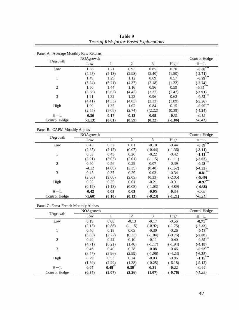
47

Table 9

Tests of Risk-factor Based Explanations

Panel A : Average Monthly Raw Returns

TAgrowth

NOAgrowth Control Hedge

Low 1 2 3 High H－L

Low

1.36 1.21 0.93 0.85 0.70 -0.80***

(4.45) (4.13) (2.98) (2.40) (1.50) (-2.71)

1

1.49 1.29 1.12 0.69 0.57 -0.99***

(5.24) (5.21) (4.37) (2.18) (1.22) (-2.74)

2

1.50 1.44 1.16 0.96 0.59 -0.85***

(5.38) (5.62) (4.47) (3.37) (1.47) (-3.91)

3

1.41 1.32 1.23 0.96 0.62 -0.82***

(4.41) (4.33) (4.03) (3.33) (1.89) (-5.56)

High

1.09 1.35 1.02 0.84 0.15 -0.95***

(2.55) (3.08) (2.74) ((2.22) (0.39) (-4.24)

H－L

-0.30 0.17 0.12 0.05 -0.31 -0.15

Control Hedge (-1.13) (0.61) (0.59) (0.22) (-1.06) (-0.41)

Panel B: CAPM Monthly Alphas

TAgrowth

NOAgrowth Control Hedge

Low 1 2 3 High H－L

Low

0.45 0.32 0.01 -0.10 -0.44 -0.89***

(2.85) (2.12) (0.07) (-0.44) (-1.36) (-3.11)

1

0.63 0.45 0.26 -0.22 -0.42 -1.11***

(3.91) (3.63) (2.01) (-1.15) (-1.11) (-3.03)

2

0.60 0.56 0.29 0.07 -0.39 -0.93***

-4.12 (4.80) (2.35) (0.48) (-1.52) (-4.52)

3

0.45 0.37 0.29 0.03 -0.34 -0.81***

(2.50) (2.66) (2.03) (0.23) (-2.05) (-5.49)

High

0.05 0.35 0.01 -0.21 -0.91 -0.97***

(0.19) (1.18) (0.05) (-1.03) (-4.89) (-4.38)

H－L

-0.42 0.03 0.03 -0.05 -0.34 -0.08

Control Hedge (-1.60) (0.10) (0.13) (-0.23) (-1.21) (-0.21)

Panel C: Fama-French Monthly Alphas

TAgrowth

NOAgrowth Control Hedge

Low 1 2 3 High H－L

Low

0.19 0.08 -0.13 -0.17 -0.56 -0.71**

(2.15) (0.88) (-1.15) (-0.92) (-1.75) (-2.33)

1

0.40 0.18 0.03 -0.30 -0.26 -0.73**

(3.85) (2.77) (0.33) (-1.84) (-0.76) (-2.08)

2

0.49 0.44 0.10 -0.11 -0.40 -0.85***

(4.71) (6.21) (1.40) (-1.17) (-1.94) (-4.18)

3

0.46 0.40 0.28 -0.08 -0.46 -0.93***

(3.47) (3.96) (2.99) (-1.06) (-4.23) (-6.38)

High

0.29 0.53 0.24 -0.03 -0.86 -1.15***

(1.39) (2.29) (1.38) (-0.25) (-6.18) (-5.12)

H－L

0.07 0.45**

0.39**

0.21 -0.22 -0.44

Control Hedge (0.34) (2.07) (2.26) (1.07) (-0.76) (-1.25)

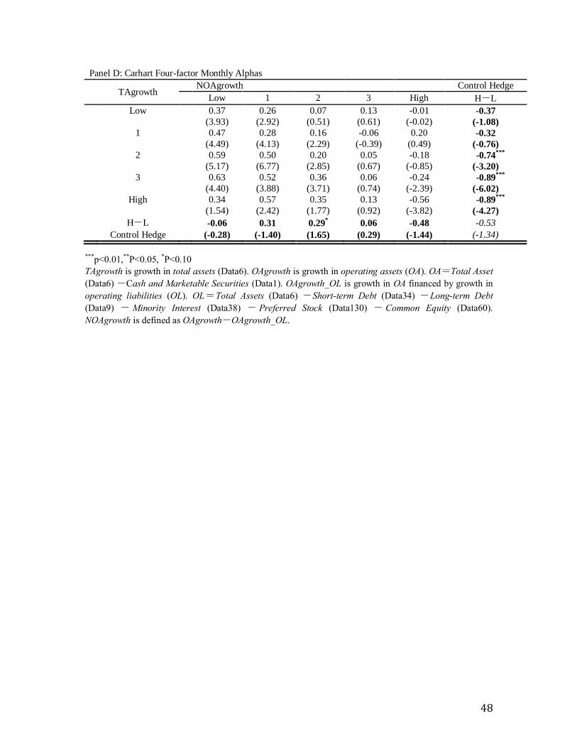
48

Panel D: Carhart Four-factor Monthly Alphas

TAgrowth

NOAgrowth Control Hedge

Low 1 2 3 High H－L

Low

0.37 0.26 0.07 0.13 -0.01 -0.37

(3.93) (2.92) (0.51) (0.61) (-0.02) (-1.08)

1

0.47 0.28 0.16 -0.06 0.20 -0.32

(4.49) (4.13) (2.29) (-0.39) (0.49) (-0.76)

2

0.59 0.50 0.20 0.05 -0.18 -0.74***

(5.17) (6.77) (2.85) (0.67) (-0.85) (-3.20)

3

0.63 0.52 0.36 0.06 -0.24 -0.89***

(4.40) (3.88) (3.71) (0.74) (-2.39) (-6.02)

High

0.34 0.57 0.35 0.13 -0.56 -0.89***

(1.54) (2.42) (1.77) (0.92) (-3.82) (-4.27)

H－L

-0.06 0.31 0.29

* 0.06 -0.48 -0.53

Control Hedge (-0.28) (-1.40) (1.65) (0.29) (-1.44) (-1.34)

***p<0.01,**P<0.05, *P<0.10

TAgrowth is growth in total assets (Data6). OAgrowth is growth in operating assets (OA). OA＝Total Asset

(Data6) －Cash and Marketable Securities (Data1). OAgrowth_OL is growth in OA financed by growth in

operating liabilities (OL). OL＝Total Assets (Data6) －Short-term Debt (Data34) －Long-term Debt

(Data9) － Minority Interest (Data38) － Preferred Stock (Data130) － Common Equity (Data60).

NOAgrowth is defined as OAgrowth－OAgrowth_OL.

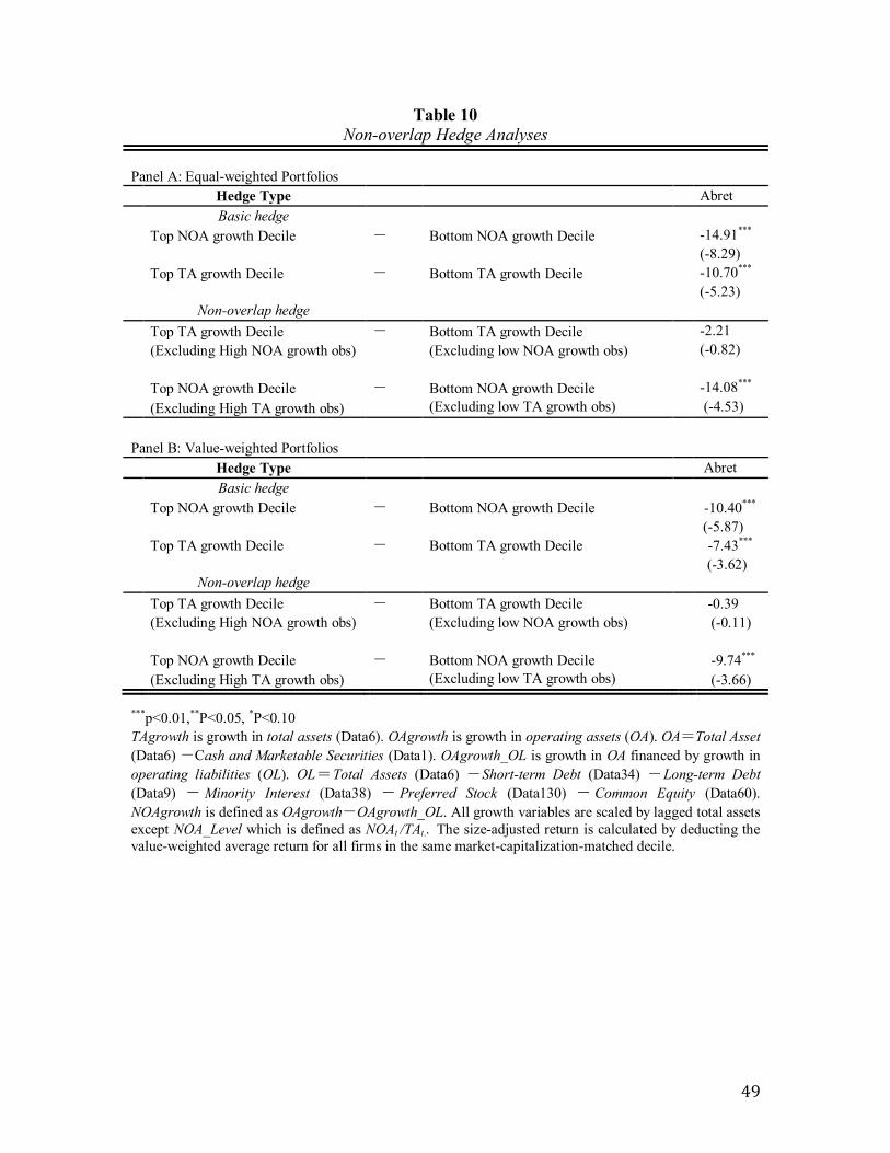
49

Table 10

Non-overlap Hedge Analyses

Panel A: Equal-weighted Portfolios

Hedge Type Abret

Basic hedge

Top NOA growth Decile － Bottom NOA growth Decile

-14.91***

(-8.29)

Top TA growth Decile － Bottom TA growth Decile

-10.70***

(-5.23)

Non-overlap hedge

Top TA growth Decile － Bottom TA growth Decile

-2.21

(Excluding High NOA growth obs)

(Excluding low NOA growth obs)

(-0.82)

Top NOA growth Decile － Bottom NOA growth Decile

-14.08***

(Excluding High TA growth obs) (Excluding low TA growth obs) (-4.53)

Panel B: Value-weighted Portfolios

Hedge Type Abret

Basic hedge

Top NOA growth Decile － Bottom NOA growth Decile

-10.40***

(-5.87)

Top TA growth Decile － Bottom TA growth Decile

-7.43***

(-3.62)

Non-overlap hedge

Top TA growth Decile － Bottom TA growth Decile

-0.39

(Excluding High NOA growth obs)

(Excluding low NOA growth obs)

(-0.11)

Top NOA growth Decile － Bottom NOA growth Decile

-9.74***

(Excluding High TA growth obs) (Excluding low TA growth obs) (-3.66)

***p<0.01,**P<0.05, *P<0.10

TAgrowth is growth in total assets (Data6). OAgrowth is growth in operating assets (OA). OA＝Total Asset

(Data6) －Cash and Marketable Securities (Data1). OAgrowth_OL is growth in OA financed by growth in

operating liabilities (OL). OL＝Total Assets (Data6) －Short-term Debt (Data34) －Long-term Debt

(Data9) － Minority Interest (Data38) － Preferred Stock (Data130) － Common Equity (Data60).

NOAgrowth is defined as OAgrowth－OAgrowth_OL. All growth variables are scaled by lagged total assets

except NOA_Level which is defined as NOAt /TAt.. The size-adjusted return is calculated by deducting the

value-weighted average return for all firms in the same market-capitalization-matched decile.