THE TRACTIVE PERFORMANCE OF A FRICTION-BASED …

THE TRACTIVE PERFORMANCE OF A

FRICTION-BASED PROTOTYPE TRACK

TINGMIN YU

Submitted in partial fulfillment of the requirements for the

Degree of

Philosophiae Doctor

in

The Faculty of Engineering, Built Environment and Information Technology

University of Pretoria

Pretoria

October, 2005

UUnniivveerrssiittyy ooff PPrreettoorriiaa eettdd –– YYuu,, TT ((22000066))

SUMMARY

THE TRACTIVE PERFORMANCE OF A

FRICTION-BASED PROTOTYPE TRACK

Supervisor: Professor H.L.M. du Plessis

Department: Civil and Biosystems Engineering

Degree: Philosophiae Doctor (Engineering)

In recent years, the interest in the design, construction and utilization of rubber tracks

for agriculture and earth moving machinery has increased considerably. The

development of such types of tracks was initiated by the efforts to invent a more

environmentally friendly vehicle-terrain system. These tracks are also the result of

the continuous effort to develop more cost-effective traction systems.

A rubber-surfaced and friction-based prototype track was developed and mounted on

the patented modification of a new Allis Chalmers four wheel drive tractor. The track

is propelled by smooth pneumatic tyres by means of rubber-rubber friction and the

tractive effort of the track is mainly generated by soil-rubber friction between the

rubber surface of the track elements and terrain.

The experimental track layer tractor, based on an Allis Chalmers 8070 tractor (141

kW) was tested on concrete and on cultivated sandy loam soil at 7.8%; 13% and 21%

soil water content. The contact pressure and the tangential force on an instrumented

track element, as well as the total torque input to one track, was simultaneously

recorded during the drawbar pull-slip tests. Soil characteristics for pressure-sinkage

and friction-displacement were obtained from the field tests by using an instrumented

linear shear and soil sinkage device.

i


By applying the approach based on the classical bevameter technique, analytical

methods were implemented for modelling the traction performance of the prototype

track system. Different possible pressure distribution profiles under the tracks were

considered and compared to the recorded data. Two possible traction models were

proposed, one constant pressure model, for minimal inward track deflection and the

other a flexible track model with inward deflection and a higher contact pressure at

both the front free-wheeling and rear driving tyres. For both models, the traction

force was mainly generated by rubber-soil friction and adhesion with limited

influence by soil shear. For individual track elements, close agreement between the

measured and predicted contact pressure and traction force was observed based on

the flexible track model.

The recorded and calculated values of the coefficient of traction based on the

summation of the traction force for the series of track elements were comparable to

the values predicted from modelling. However, the measured values of drawbar pull

coefficient were considerably lower than the predicted values, largely caused by

internal track friction in addition to energy dissipated by soil compaction. The

tractive efficiency for soft surface was also unacceptably low, probably due to the

high internal track friction and the low travel speeds applied for the tests.

The research undertaken identified and confirmed a model to be used to predict

contact pressure and tangential stresses for a single track element. It was capable of

predicting the tractive performance for different possible contact pressure values.

Key terms: adhesion, contact pressure, rubber track, soil-rubber friction, traction,

traction modelling, tractive performance.

ii


ACKNOWLEDGEMENTS

I wish to express my appreciation to Professor H.L.M. du Plessis, my supervisor, for

his instruction, advice, support and encouragement throughout my study and work.

Appreciation is also expressed to the following people for their valuable advice and

help:

• Mr. C. du Toit, Agricultural Engineering Workshop Manager.

• Mr. J. Nkosi, Mr. D. Sithole and Mr. W. Morake, Technical Assistants in the

Agricultural Engineering Workshop.

• Dr. R. Sinclair for reviewing the manuscript.

Finally, appreciation is expressed to my wife, my children and my parents for their

love, support, encouragement and sacrifice.

iii


TABLE OF CONTENTS

Page SUMMARY………………………………………………………………………………...……….....i ACKNOWLEDGEMENTS……………………………………………………………...….…......iii TABLE OF CONTENTS…………………………………………………………...……………..iv NOMENCLATURE……………………………………………………………...………………...viii

CHAPTER I INTRODUCTION……………………………………………………………………….......……..1-1

1.1 Developments in terrain-vehicle mechanics…….……….……………………..….......1-1

1.2 Optimization of new traction systems………………………..…………………….........1-2

1.3 The prediction and evaluation of tractive performance…………………………...…...1-4

1.4 The development of a prototype track and the motivation for the research……...…1-4

CHAPTER II LITERATURE REVIEW………………..………………………………………………….…….2-1 2.1 Soil characterization for traction modelling……………………………………..………2-1

2.1.1 The cone penetrometer technique for soil characterization……………..…2-2

2.1.2 The bevameter technique for soil characterization……………………..…….2-4

2.1.2.1 Measurement of pressure-sinkage relationships……………..…….2-5

2.1.2.2 Measurement of soil shear characteristics……………………...…...2-9

2.1.3 Friction and adhesion characterization for the soil-rubber

contact surface………………………………………………………………….2-14

2.2 Traction performance modelling for wheeled vehicles……………………………….2-16

2.2.1 Empirical methods for traction performance modelling…………………..2-16

2.2.2 Analytical methods for traction performance modelling…………………..2-19

2.3 Traction performance modelling for tracked vehicles………………………...…….2-23

2.3.1 Empirical methods for traction performance modelling…………………..2-23

2.3.2 Analytical methods for traction performance modelling…………………..2-23

2.4 Development of and traction characteristics for rubber tracks………………….…..2-30

2.5 Measurement of the distribution of contact

and tangential stresses below a track……………………………………………….2-35

2.5.1 Track link dynamometer by Wills (1963)……………………….…………....2-35

2.5.2 Applications of extended octagonal ring transducers

for measuring two perpendicular forces…………………...…………………2-36

2.6 Development of the prototype traction system based on soil-rubber friction ….…2-38

2.7 Justification for conducting this study………………………………………………….2-40

iv


2.8 Objectives…………………….…………………………………………………..……….2-41

CHAPTER III CONSTRUCTION OF THE PROTOTYPE RUBBER-FRICTION TRACTION SYSTEM……………………….………………….....3-1 3.1 Introduction…………………………………………………………………...…………….3-1

3.2 The prototype track…………………………………………………………...…………...3-3

3.2.1 The fundamental construction and layout……………………….…………...3-3

3.2.2 The centre ground wheels…………………………………………….……….3-6

3.2.3 Track mounting, tensioning and driving friction at interface……………….3-6

3.2.4 The beam effect……………………………………………………..…………..3-7

3.3 The drive train, steering control and automatic differential lock…………..………….3-8

3.4 Dimensions of the prototype track……………………………………………………3-11

3.5 Preliminary tests and assesment of tractive performance ………………………..…3-11

3.6 Summary and remarks……………………...……………………………………….…..3-13

CHAPTER IV DEVELOPMENT OF THE TRACTION MODEL FOR THE PROTOTYPE TRACK …………………………………………………….……....4-1 4.1. Introduction…………………………………………………………………………..….….4-1

4.2 Characterization of rubber-soil friction and soil shear with displacement………...…4-2

4.3 Characterization of the relationship between contact pressure and sinkage……...4-5

4.4 Analysis of the distribution of track-soil contact pressure…………………………….4-6

4.4.1 Tractive effort for uniform and trapezoidal pressure distribution.……..…..4-6

4.4.2 Tractive effort for a rigid track model with a tilt angle…………………..…..4-10

4.4.3 Tractive effort for the flexible track model ...…………...…………..………..4-12

4.5 The prediction of motion resistance ………………………………………...…………4-18

4.6 Internal resistance and the friction drive between the wheel and the track………4-20

4.7 Total drawbar pull of the prototype track………………………………………………4-22

4.8 The coefficient of traction and tractive efficiency …………………………………....4-22

4.9 Modelling procedure …………………..………………………………….……..…...4-23

CHAPTER V INSTRUMENTATION, CALIBRATION AND EXPERIMENTAL PROCEDURE…...5-1 5.1 Introduction……………………………………………………………………………….5-1

5.2 Apparatus for soil characterization……………………………………………..………..5-2

5.3 The extended octagonal ring transducers for measuring

v


the distribution of contact pressure and tangential stress………….………………..5-6

5.3.1 Design of the transducer……………………………………………..………5-6

5.3.2 Calibration and installation of the transducers…………………..…………5-8

5.4 Instrumentation for measuring torque, slip and drawbar pull ……………………...5-13

5.4.1 Instrumentation for measuring the side shaft torque……………..………...5-13

5.4.2 Instrumentation for measuring speed and slip…..………………………….5-15

5.4.3 Instrumentation for measuring drawbar pull………………………………..5-18

5.5 The computerized data logging system….……………………………..…………..5-19

CHAPTER VI FIELD EXPERIMENTS AND DATA COLLECTION……………………………………..6-1

6.1 Measurement of soil properties …………………………………………….…………...6-1

6.1.1 Soil classification……………………………………………..……….………….6-1

6.1.2 Soil density, soil water content and cone index………………………….…..6.1

6.2 Experimental procedure for soil characterization……………………………………....6-2

6.2.1 Pressure-sinkage characterization for the test plot………………………….6-2

6.2.2 Soil-rubber frictional and soil shear characterization ……………….………6-6

6.3 Drawbar pull tests and data collection…………………………………………………6-10

CHAPTER VII RESULTS, ANALYSIS AND MODEL VALIDATION ………………..…………………7-1

7.1 Introduction……………………………………………………………………………….7-1

7.2 The distribution of contact pressure …………………………………………………...7-1

7.2.1 The contact pressure distribution and frictional stress on a hard surface..7-1

7.2.2 The effect of the ground wheels on the pressure distribution

and frictional stress for a hard surface……………..………………………….7-4

7.2.3 The contact pressure distribution and frictional stress

on a soft surface with zero drawbar pull………………..……………………..7-5

7.2.4 The effect of the ground wheels on the contact pressure distribution

and frictional stress for a soft surface…………..……………………………..7-7

7.2.5 The influence of the soil water content and the drawbar pull

on the contact pressure distribution………………..………………………….7-9

7.3 The relationships of traction coefficient and total slip…………………..……….....7-14

7.4 The tractive efficiency…………………………………..……………………..…………7-17

7.5 Analysis of the factors affecting the tractive performance………….….……………7-19

7.5.1 Soil water content……………….………………………………..…………..7-19

7.5.2 Track tension……………………………..……………………………………..7-19

7.5.3 Motion resistance and internal friction…………………………………....7-20

vi


CHAPTER VIII SUMMARY, CONCLUSIONS AND RECOMMENDATIONS………………..………....8-1 8.1 Summary……………………………………………………………………..………...8-1

8.2 Conclusions…………………………………………………………………..…..………..8-2

8.3 Recommendations………………………………………………………………………..8-4

LIST OF REFERENCES…………………………………………………………….………….…1

APPENDIX A…………………………………………………………………………….………..…7

vii


NOMENCLATURE

A contact area, (m2).

b track contact width, (m).

bo width of octagonal ring transducer, (m).

bt tyre section width, (m).

bw width of wheel, (m).

C constant to relate the entrance and the exit angles.

Ca a constant to calculate the actual speed based on rd and π.

Cct coefficient of traction.

Ct a constant to calculate the theoretical speed based on rd and π.

c soil cohesion, (Pa).

ca soil-rubber adhesion, (Pa).

D wheel diameter, (m).

d tyre diameter, (m).

E modulus of elasticity of octagonal ring transducer material, (Pa).

e eccentric distance of centre of gravity in longitudinal direction, (m).

F force, (N).

Fh drawbar pull, (N).

Fhi longitudinal force on i-th track segment, (N).

Fhmax maximum drawbar pull, (N).

Ft tractive force, (N).

Fti tractive force for i-th track segment, (N).

Ftmax maximum tractive effort, (N).

Fx force in horizontal direction, (N).

Fy force in vertical direction, (N).

fa frequency recorded by ground speed sensor.

ft frequency recorded by theoretical speed sensor.

G sand penetration resistance gradient, (Pa/m).

H horizontal force, (N).

h height, (m).

i slip as decimal.

viii


j tangential displacement, (m).

K tangential deformation modulus, (m).

K1, K2 empirical constants for soil shear.

Kr ratio of the residual shear stress τr to the maximum shear stress τmax.

Kω shear displacement where the maximum shear stress τmax occurs, (m).

kF constant for measuring force F for extended octagonal ring transducer.

kP constant for measuring force P for extended octagonal ring transducer.

kc Bekker sinkage parameter related to cohesion, (kN/mn+1).

kφ Bekker sinkage parameter related to internal soil friction, (kN/mn+2 ).

kc′ and kφ′ dimensionless constants related to pressure-sinkage tests.

L track contact length, (m).

Lo half distance between two circular centres of extended octagonal ring

transducer, (m).

Lt average travel distance, (m).

ℓ length, (m).

ℓ t contact length, (m).

ℓ i track length represented by i-th track segment, (m).

Ncs wheel numeric.

Nt revolutions of drive wheel.

n exponent of terrain deformation for Bekker sinkage equations

np number of periods.

P force, (N).

Pin input power, (kW).

Pout output power, (kW).

p contact pressure, (Pa).

p1 contact pressure at the front of the track, (Pa).

p2 contact pressure at the rear of the track, (Pa).

pc pressure due to stiffness of the tyre carcass, (Pa).

pi contact pressure for i-th track segment, (Pa).

pti tyre inflation pressure, (Pa).

p(x) contact pressure on track at distance x (meter) from front, (Pa).

R radius of deformed track between front and rear tires, (m).

ix


Rc motion resistance due to soil compaction, (N).

Re external track resistance, (N).

Ri internal track resistance, (N).

Rr total motion resistance, (N).

r wheel radius, (m).

rd effective radius of the drum to measure ground speed, (m).

ri radius for i-th track segment, (m).

ro mean radius of octagonal ring, (m).

rr rolling radius of wheel, (m).

rt effective rolling radius of the track drive wheel, (m).

St total slip of track as decimal.

T torque, (N·m).

T0 track pre-tension, (N).

t time, (second).

to thickness of octagonal ring transducer, (m).

V forward velocity of tractor, (m/s).

Va absolute velocity, (m/s).

Vj slip velocity, (m/s).

Vt theoretical velocity, (m/s).

W total vertical load, (N).

Wf vertical load on front wheels, (N).

Wi vertical load on i-th track segment, (N).

Wr vertical load on rear wheels, (N).

X projected distance in horizontal direction, (m).

x distance, (m).

Z vertical difference in height of contact circle between front and rear

wheels, (m).

Zr depth of rut, (m).

z sinkage, (m).

z0 wheel sinkage, (m).

zf sinkage of track front, (m).

zf0 initial sinkage of track front, (m).

x


zr sinkage of track rear, (m).

zt track sinkage, (m).

α angle, (rad).

α1f entrance angle of front tire, (rad).

α2f exit angle of front tire, (rad).

α1r entrance angle of rear tire, (rad).

α2r exit angle of rear tire, (rad).

αi entrance angle of i-th track segment, (rad).

αi+1 exit angle of i-th track segment, (rad).

β tilt angle, (rad).

γs unit weight of soil, (N/m3).

δ angle of rubber-soil friction, (degree).

εφP strain caused by force P.

εφF strain caused by force F.

η tractive efficiency.

θ angle, (rad).

θ0 wheel entrance angle, (rad).

μ traction coefficient.

μg gross traction coefficient.

μφ friction coefficient between contact surfaces.

π wrap angle, (180°).

ρ motion resistance ratio.

σ contact pressure, (Pa).

τ shear stress, (Pa).

τf frictional stress, (Pa).

τfi frictional stress for i-th segment of track, (Pa).

τfmax maximum frictional stress, (Pa).

τmax maximum shear stress, (Pa).

τr residual shear stress, (Pa).

φ angle of soil internal shearing resistance, (degree).

xi


φF nodal angle for measuring force F on octagonal rings, (degree).

φP nodal angle for measuring force P on octagonal rings, (degree).

ψ tyre deflection, (m).

ω angular velocity, ( rad/s).

ωd angular speed of the drum for measuring ground speed, (rad/s).

ωt theoretical angular velocity, (rad/s).

xii


CHAPTER 1 _________________________________________________________________________________

CHAPTER I

INTRODUCTION

1.1 DEVELOPMENTS IN TERRAIN-VEHICLE MECHANICS

For a long period, one of the challenges in the design of an off-road vehicle was to

equip it with a traction device that can develop high traction efficiently with the

minimum soil degradation. The aim of terrain-vehicle mechanics is to provide guiding

principles to obtain a better understanding of the interaction of the soil-vehicle system.

The studies of terrain-vehicle mechanics are generally directed toward the problems

most frequently encountered in the categories of (Yong, 1984):

excessive soil compaction induced by vehicle traffic;

excessive wheel or track sinkage due to the imposed ground pressure and

physical characteristics of both the soil and the vehicle; and

excessive wheel or track slippage and insufficient traction caused by internal

soil shear or surface friction failure.

Generally, terrain-vehicle mechanics can be divided into three highly interdependent

areas as shown in Figure 1.1. Traffic ability and terrain characterization is concerned

with the ability of the terrain surface to support vehicle traffic and the environmental

consequences of damage to the terrain. Performance prediction and evaluation for a

vehicle is the core issue when one considers the vehicle and the environment as an

integral system to be optimized. The vehicle design considerations are relevant to the

design parameters and specifications of the vehicle.

1-1


CHAPTER 1 _________________________________________________________________________________

Traffic abilityand terrain

characterization

Performance prediction andevaluation

Vehicle designconsiderations

Terrain-vehicle traction mechanics

Figure 1.1. The related areas of terrain-vehicle mechanics (Yong, 1984)

1.2 OPTIMIZATION OF NEW TRACTION SYSTEMS

In the past, the choice of conventional tractive elements used for off-road vehicles to

generate tractive effort was mainly restricted to either pneumatic tyres or steel tracks.

It is commonly recognized that tracked vehicles are better draught tractors because

they are capable of producing high drawbar pull at a lower slip value and high tractive

efficiency, even under difficult conditions such as on very soft surfaces. The large

ground contact areas of the tracks result in low ground pressure and good stability on

steep slopes. However, steel tracks have adverse characteristics when compared to

pneumatic tyres from the point of view of steerability, manoeuvrability, noise, driver

fatigue, maintenance and limited speeds. Additionally, travel on public roads is

restricted in most areas due to road surface damage from penetration by the steel track

grousers.

The worldwide use of steel-tracklayer tractors in the agricultural sector has declined

since the introduction of large four-wheel-drive tractors. Four-wheel-drive tractors are

characterized by moderate drawbar pull, high speeds, better ergonomics and good

1-2


CHAPTER 1 _________________________________________________________________________________

performance, increasing the productivity over steel-tracked ones. Pneumatic tyres also

allow comparatively high speed traveling on public roads. With low-pressure tyres

fitted onto wheeled tractors, the compaction of soil can also be reduced.

For many years there has been an interest in developing rubber tracks to be used on

tractors to combine the good tractive performance and low ground pressure of the steel

tracks with the non-abrasive features, higher speeds, and asphalt road-going capability

of the pneumatic tyres. In recent years, the availability of rubber compounds and

methods of steel reinforcement enabled manufacturers to construct rubber tracks of

adequate strength and durability for use on agricultural tractors and even earth moving

machines. These tracks are cost effective and lighter than the conventional steel tracks.

When summarized and compared to steel tracks, rubber tracks offer additional

advantages such as:

lower noise and less hazardous vibration levels for the operator;

relative simplicity and lighter construction;

ability to be used on asphalt roads without damage to the road surface; and

higher operating speeds.

The Caterpillar Challenger series of tractors represents the most successful use of

rubber tracks.

Bridgestone’s positive drive rubber-covered steel tracks, driven by sprockets are also

popularly used, especially for the cases of modified conventional undercarriages.

The development of alternative types of traction systems is a continuous process for

many research workers, striving for better traction characteristics with less

compaction or other damage to the terrain.

1-3


CHAPTER 1 _________________________________________________________________________________

1.3 THE PREDICTION AND EVALUATION OF TRACTIVE

PERFORMANCE

M. G. Bekker (1956, 1960, 1969) pioneered the theoretical investigation into the

tractive mechanism for off-road vehicles. Although numerous attempts and

considerable progress has been made in the past few decades to quantify the

soil-machine interaction, understanding of this phenomenon is still far from

satisfactory. Generally, models for prediction and evaluation of traction performance

can be currently categorized as:

empirical models;

semi-empirical models; and

analytical models.

All three methods have been used for modelling the traction of both wheeled and

tracked vehicles, with various advantages and disadvantages. The details of the

research undertaken by different researchers will be reviewed in Chapter 2.

1.4. THE DEVELOPMENT OF A PROTOTYPE TRACK AND

THE MOTIVATION FOR THE RESEARCH

In an effort to pursue comprehensively balanced running gear for a traction vehicle to

be used in agriculture, construction and military sectors in South Africa, a prototype

track was developed with the feature of cable-tightened and rubber-covered steel track

elements. The track is driven by smooth pneumatic tyres through rubber-rubber

friction. The tractive effort of the track is also developed by soil-rubber friction and to

a limited extent shear between the rubber surface of the track elements and terrain

surface. Based on the walking beam concept, the track was developed to achieve a

more uniformly distributed and lower vertical contact pressure, thus reducing motion

resistance and soil compaction, resulting in better tractive efficiency at lower track slip

values.

1-4


CHAPTER 1 _________________________________________________________________________________

The aim of the design concept was to achieve greatly improved tractive performance,

reduced motion resistance and soil compaction, comparable to that of a rubber crawler

tracks working on soft terrain surface. This will reduce the operation cost and increase

the yield of agriculture, therefore providing a significant advantage in agricultural

production.

One of the important construction features for this prototype friction-based track is

that it is composed out of a number of rubber covered track elements which enables

low-cost replacement and maintenance when the track is partly damaged. Most of the

currently in use rubber tracks are constructed as one integral single piece, i. e. a steel

reinforced rubber belt, necessitating a costly replacement of the complete unit, if

partly damaged.

As for other wheeled and steel-tracklayer tractors, the evaluation and performance

prediction for a vehicle equipped with this prototype track is of great interest. It will

assist in further validation, design modifications and optimum application of the new

track system.

1-5


CHAPTER 2 _________________________________________________________________________________

CHAPTER II

LITERATURE REVIEW

2.1 SOIL CHARACTERIZATION FOR TRACTION MODELLING

For off-road vehicle engineering the measurement of the soil properties is one of the

fundamental tasks for the prediction and evaluation of tractive performance.

Performance evaluation of terrain-vehicle systems involves both the design

parameters for the vehicle and the measurement and evaluation of the physical

environment within which the vehicle operates. The soil mechanical properties can be

categorized as soil physical properties and soil strength parameters.

Soil physical properties affect the tractive performance of a vehicle by changing the

soil strength characteristics under different conditions. However, a universal standard

method does not yet exist for the measurement of the specific soil parameters. The

classification and the measurement of the soil physical properties therefore depend

much on the requirements of the individual user.

By utilizing the basic concepts from geotechnical and civil engineering, Karafiath &

Nowatzki (1978) quoted an extensive range of references, definitions and

measurements of permanent and transient soil properties for off-road vehicle

engineering. Among the soil physical properties described by Karafiath & Nowatzki

(1978) and Koolen & Kuipers (1983), some are usually necessary for traction such as

soil classification by composition, soil porosity, soil water content, and soil density.

When the vehicle travels over a soft terrain surface, soil strength parameters are the

major factors affecting the supporting, floating, shear, friction and other abilities of the

soil under the vehicle load. The prediction of off-road vehicle performance, to a large

2-1


CHAPTER 2 _________________________________________________________________________________

extent, depends on the proper evaluation and measurement of the strength parameters

of the terrain which has been one of the major objectives of terrain-vehicle mobility

research.

In geotechnical engineering, the standard methods for measuring soil strength

parameters usually involve laboratory experiments, carried out on relatively small soil

samples. In off-road vehicle engineering, if the soil strength and deformation

characteristics are to be closely related to the field conditions under which the

performance of the vehicles are evaluated, it is essential to measure the soil parameters

in the field. The techniques currently in use for measuring and characterizing in-situ

soil strength properties including the cone penetrometer (ASAE, 1988), bevameter

(Bekker, 1969; Wong, 1993) and other techniques (Chi, Tessier, McKyes & Laguë,

1993), adopted from civil engineering.

In the highly theoretical models, utilizing the elastic-plastic theory and the finite

element method (Chi, Kushwaha & Shen, 1993; Shen & Kushwaha, 1998), the soil

parameters are usually measured by laboratory experiments, adapted from civil

engineering such as a triaxial test and a direct shear test. As much as eight parameters

may need to be measured under laboratory conditions before the development of the

model (Chi, Kushwaha & Shen, 1993). This probably is the reason why the purely

theoretical methods have not been used extensively for practical applications.

Therefore, for the in-situ measurement in the field, the cone penetrometer and

bevameter techniques are still the two most frequently used for soil characterization

for traction and mobility modelling.

2.1.1 The cone penetrometer technique for soil characterization

The cone penetrometer used to evaluate soil strength for trafficability studies was

initially applied by the U.S. Army Engineer Waterways Experimental Station (WES)

(Freitag, 1965). To interpret and compare the results, the design and use of the cone

penetrometer for agricultural applications is standardized as ASAE S313.2 (ASAE,

2-2


CHAPTER 2 _________________________________________________________________________________

1988). This ASAE standard also specifies the index application range for different

penetrometer types, penetration speed and depth increments for soil characterization.

The penetrometer consists of a circular 30° stainless steel cone mounted on a circular

stainless steel shaft as shown in Figure 2.1. Other standardized dimensions of the

penetrometer and the components are also shown in Figure 2.1.

Figure 2.1. Cone penetrometer standardized by the ASAE S313.2.

The value of “Cone Index (CI)” represents the average penetration force per unit

projected cone base area exerted by the soil upon the conical head when forced down

to a specific depth at a penetration rate of about 3 cm/s as recommended by the ASAE

standard S313.2 (ASAE, 1988). The cone index constitutes a compound parameter

reflecting the comprehensive influence of shear, compression and even soil-metal

friction.

The CI values may vary considerably with depth (Wismer & Luth, 1973). Therefore,

the CI values usually used for traction prediction are the average value recorded over a

depth corresponding to the maximum tyre or track sinkage.

2-3


CHAPTER 2 _________________________________________________________________________________

For many years, the penetration test remained a very popularly used method applied by

researchers for soil compaction and for some empirical traction studies. It is not only

because of simplicity, convenience and ease of use, but also the provision of valuable

information about the mechanical state of the soil. The value of such information can

best be assessed when the CI is correlated to other information or parameters obtained

from other test devices such as triaxial tests or the bevameter techniques. Although the

CI value is important for soil characterization, it is questionable whether only the one

value of CI is sufficient to represent the sophisticated phenomenon of soil reaction

under vehicle traffic.

2.1.2 The bevameter technique for soil characterization

The bevameter technique, originally developed by Bekker (1956, 1960 and 1969) is

well documented for characterizing soil strength and soil sinkage parameters relevant

to tractive performance. Since a traction device or running gear applies both contact

pressure and tangential stresses to the terrain surface to develop tractive effort, it

seems reasonable to simulate the real phenomenon by applying loads in both

directions. The bevameter technique attempts to represent this situation better than

other currently available techniques (Wong, 1989, 1993).

The bevameter technique consists of:

a plate sinkage test to determine the pressure-sinkage relationships of the soil;

and

a shear test to determine the in situ shear strength parameters of the soil.

A complete bevameter is illustrated schematically in Figure 2.2.

2-4


CHAPTER 2 _________________________________________________________________________________

Figure 2.2. Schematic layout of a bevameter (Wong, 1993).

2.1.2.1 Measurement of pressure-sinkage relationships

By forcing rigid steel plates of different diameters or widths for rectangular plates into

the soil surface for the specific test site, a typical family of pressure-sinkage curves can

be generated as shown in Figure 2.3. In order to characterize the pressure-sinkage

relationship for homogeneous terrain, the following equation was proposed by Bekker

(1956):

(2.1)

where

p = contact pressure, (Pa).

b = width of a rectangular sinkage plate or radius of a circular sinkage plate, (m).

z = sinkage, (m).

kc, kφ and n = empirically determined pressure-sinkage soil characteristics.

c

bk(p = n)zkφ+

2-5


CHAPTER 2 _________________________________________________________________________________

In equation (2.1), kc and kφ have dimensional terms of N/mn+1 and N/ mn+2 respectively

and the parameters are related to soil cohesion and internal friction. The values of p

and z are measured while the parameters kc, kφ and n are derived by fitting

experimental data to the above equation (2.1) (Wong, 1989, 1993).

Figure 2.3. Typical pressure-sinkage curves (Bekker, 1969).

To obtain the parameters in equation (2.1), the results of a minimum of two tests with

two plates having different widths or radii are required. The two tests produce two

curves represented by two equations that can be rewritten in logarithmic form. They

represent two parallel straight lines of the same slope on the log-log scale, where n is

the slope of the lines. The values of kc and kφ are then calculated from the contact

pressure for the two plates at z=1 (Wong, 1989).

It often happens that the pressure-sinkage curves may not be quite parallel on the

log-log scale, probably due to the nonhomogeneity of the terrain and possible

experimental errors. It is recommended by Wong (1989) that under the circumstances

of two n values, the mean of the two values is usually accepted as the correct n value.

To improve the speed and efficiency of measurement and soil characterization for the

bevameter technique, Wong (1980, 1989) developed a more rigorous and automated

2-6


CHAPTER 2 _________________________________________________________________________________

data processing approach based on the weighted least squares method to derive the

values of n, kc and kφ. In Wong’s processing approach, the parameters in relation to

repetitive pressure-sinkage loading-unloading were also taken into consideration.

Although the technique improved the efficiency of obtaining kc, kφ and n, inherent

problems still exist such as differences in behavior of a metallic plate compared to that

of a rubber tyre or track, the effect of strain rate, speed of penetration and the fact that

the plate can only characterize surface soil characteristics. The parameters kc and kφ in

equation (2.1) also depend on the value of the exponent n.

To simplify equation (2.1) dimensionally, Reece (1965-1966) proposed the following

alternative equation for the pressure-sinkage relationship:

(2.2) nsc b

zbkckp ))(''( φγ+=

where

kc′, kφ′ and n = dimensionless constants.

γs = unit weight of soil, (N/m3).

c = soil cohesion, (Pa).

He also carried out a series of penetration tests to verify the validity of the principal

features of the above equation. The sinkage plates used by Reece had various widths

with aspect ratios of at least 4.5.

To measure the soil shear strength parameters, Reece (1965-66) built the apparatus as

shown in Figure 2.4. One of the advantages of Reece’s method and apparatus was that

the sinkage caused by shear or so called slip-sinkage was also taken into consideration.

2-7


CHAPTER 2 _________________________________________________________________________________

Figure 2.4. Reece’s linear shear apparatus to measure soil shear strength and sinkage

(Reece, 1965-1966).

Wong (1989) proved for various mineral terrains tested that the values of n, in both

Bekker’s equation and Reece’s equation, were identical. It was also indicated that

almost the same goodness-of-fit is resulted by fitting the same set of pressure-sinkage

data with equation (2.1) or equation (2.2). Therefore, both Bekker’s and Reece’s

equations were of similar form and comparable for the mineral terrain encountered for

most operating conditions. As the bevameter technique was simpler and the

parameters were easier to record and process, the bevameter method was more

popularly used for traction studies.

Youssef and Ali (1982) reported that the accuracy of the plate sinkage analysis was

affected by the size and shape of the plate used, as well as the soil strength parameters.

They concluded that in order to achieve a more realistic result, the plate penetration

rates ought to always be uniform and at a speed so as to simulate the situation under a

track or a wheel. However, in practice, it was difficult to apply the load at such a high

loading rate so as to simulate traffic. It was proved that the results from circular and

rectangular sinkage plates were comparable.

2-8


CHAPTER 2 _________________________________________________________________________________

Other researchers (Sela and Ehrlich, 1972; McKyes and Fan, 1985; Holm et al, 1987;

Okello, 1991) also evaluated and investigated various pressure-sinkage relations for

soil characterization. They were either very similar to Bekker’s method or more

complicated in processing than Bekker’s method. Currently, the pressure-sinkage

relationship, as proposed by Bekker, is still the popularly used expression for traction

and is therefore chosen for the research.

2.1.2.2 Measurement of soil shear characteristics

Soil shear characterization is the second test constituting the bevameter technique. By

the analysis of Bekker, a vehicle applies a shear to the terrain surface through its

running gear, which results in the development of thrust and associated slip. To

determine the shear strength of the terrain and to predict the tractive performance of an

off-road vehicle, it is essential to measure the shear stress versus shear displacement

relationship under various contact pressure conditions.

Bekker (1956) initially proposed the following equation to describe the shear stress

versus shear displacement relationship for “brittle” soils with shear diagrams of a form

similar to the aperiodic damped vibration:

(2.3)

)(tan

)(

12

2212

22

12

2212

22

)1()1(

)1()1(max

jKKKjKKK

jKKKjKKK

eeY

c

eeY

−−−−+−

−−−−+−

−+

=

−=

φσ

ττ

where

τ = shear stress, (Pa).

τmax = maximum shear stress, (Pa).

c = soil cohesion, (Pa).

φ = angle of soil internal shearing resistance, (degree).

σ = contact pressure, (Pa).

K1, K2 = empirical constants for soil shear.

j = shear displacement, (m)

2-9


CHAPTER 2 _________________________________________________________________________________

Y = the maximum value of the expression within the bracket.

Based on the data for a large number of field shear tests on a variety of natural terrain

surfaces, Wong (1989, 1993) concluded that three basic forms of shear stress-shear

displacement relationships, which varied from Bekker’s basic equation, were

encountered.

A. The first type of the shear stress-shear displacement relationship exhibited the

characteristics that the shear stress initially increased sharply and reached a “hump” of

maximum shear stress at a particular shear displacement, and then decreased and

approached a more or less constant residual value with a further increase in shear

displacement (Figure 2.5). This type of shear curve may be expressed by:

)e1(e]1)e1(K

1[1K K/jK/j11

rrmax

ωωττ −−− −−

−+= (2.4)

where Kr is the ratio of the residual shear stress τr to the maximum shear stress τmax and

Kω the shear displacement where the maximum shear stress τmax occurs.

Figure 2.5. A shear curve exhibiting a peak and constant residual shear stress

(Wong, 1989).

2-10


CHAPTER 2 _________________________________________________________________________________

2-11

B. The second type of soil stress versus shear displacement relationship exhibited the

characteristics that the shear stress increased with the shear displacement and reached

a “hump” of maximum shear stress, and continued to decrease with a further increase

in shear displacement as shown in Figure 2.6. It may be described by the following

equation:

ω

ωττ KjeKj /1max )/( −= (2.5)

where Kω is the shear displacement where the maximum shear stress τmax occurs. The

rest of the symbols are as defined for equation (2.3).

Figure 2.6. A shear curve exhibiting a peak and decreasing residual shear stress

(Wong, 1989).

C. The third type of shear stress-shear displacement relationship was another modified

version of Bekker’s equation [equation (2.3)] containing only one constant. It was

proposed by Janosi and Hanamoto (1961) as an exponential function. In practice, it is

still the most popularly used expression.

)1)(tan(

)1(/

/max

Kj

Kj

ec

e−

−

−+=

−=

φσ

ττ(2.6)

where K is referred to as the shear deformation modulus.


CHAPTER 2 _________________________________________________________________________________

2-12

This relation did not display a hump but the shear stress increased with shear

displacement and approached a constant value with a further increase in shear

displacement as shown in Figure 2.7. The value of K determines the shape of the shear

curve. Practically, the value of K can be measured directly from the shear curve or

obtained from the calculation of the slope of the shear curve at the origin by

differentiating τ with respect to j in equation (2.6):

Ke

Kdjd

j

Kj

j

max0

/max

0

τττ==

=

−

=

(2.7)

Figure 2.7. A shear curve exhibiting a simple exponential form (Wong, 1989).

The maximum shear stress for the curve is referred to as soil shear strength. The

relation between the maximum shear stress and the corresponding contact pressure can

be adequately described by the Mohr-Coulomb equation:

(2.8) φστ tanmax += c

By plotting the measured values of the maximum shear stress versus the values of the

corresponding applied contact pressure, a straight line may be obtained as shown in

Figure 2.8. Therefore, the angle of soil internal shear φ and the soil cohesion c can be

determined respectively by the slope of the straight line and the intercept of the

straight line with the shear stress axis. Based on a large number of test results as shown


CHAPTER 2 _________________________________________________________________________________

in Figure 2.8, Wills (1963) concluded that the shear strength parameters obtained from

various shearing devices including the translational shear box, shear ring, rectangular

shear plate, and rigid track were comparable.

Figure 2.8. Shear strength of sand determined by various methods

(Wills, 1963).

Summarized from the above literature review, it is obvious that the in situ

measurement methods are preferable to the laboratory methods from the point of view

of minimum disturbance of the soil sample. Furthermore, the in situ methods represent

the real soil state in the field better than the methods of samples tested in a laboratory.

The cone penetrometer is perhaps the simplest in situ method and the most widely used

technique. However, as only one parameter is used to describe the sophisticated

phenomenon, the cone index is not sufficient to replace the soil strength parameters for

representing the interaction between the running gear and the terrain surface. Despite

its limitations to interpret the comprehensive soil property, the cone penetrometer with

further modification and validation can efficiently be used for traction prediction.

Alternatively it is also more suitable for the evaluation of soil compaction studies.

2-13


CHAPTER 2 _________________________________________________________________________________

2.1.3 Friction and adhesion characterization for the soil-rubber contact surface

When a rubber tyre travels on a comparatively hard surface or a rubber track with a

smooth surface travels on a terrain surface, minimal shear action occurs within the soil.

The soil-rubber friction and the adhesion at the contact surface are the dominant

factors for developing tractive thrust. Thus the characterization of rubber-soil friction

and adhesion is of importance in developing a traction model for the track.

For describing the maximum friction and adhesion between a solid material surface

and soil, the following equation, proposed by Terzaghi (1966), can be used:

(2.9) δτ tanpcamaxf +=

Where

τfmax = maximum friction stress, (Pa).

ca = adhesion on the contact surface, (Pa).

p = normal pressure, (Pa).

δ = angle of friction between the rubber surface and soil, (degrees).

Equation (2.9) has the same form as equation (2.8), but the terms are different in

physical definition.

Neal (1966) reported results of an investigation to compare the parameters in

equations (2.8) and (2.9). As shown in Table 2.1, he concluded that the coefficient of

soil to rubber friction, tan δ was, if not exactly the same, only slightly different from

the coefficient of internal soil shear resistance, tan φ. However, the adhesion between

rubber and soil ca was less than the internal cohesion of the soil c, except for sand with

both values negligibly small, which was not listed in the data. The value of ca changed

considerably with the soil water content. Reece’s (1965-1966) research lead to the

same conclusion as Neal’s. This indicates that in sandy soils, where the values of

rubber-soil friction coefficient are similar to the values of the coefficient of soil

2-14


CHAPTER 2 _________________________________________________________________________________

internal shear resistance, the performance of a friction-based traction device is

expected to be almost similar to that of shear-based traction device.

Table 2.1. Comparison of soil internal shear and soil-rubber frictional parameters

(Neal, 1966).

Soil water

content, %

Internal

frictional angle

for soil shear φ,

degrees

Soil internal

cohesion c,

kPa

Soil-rubber

frictional angle

δ, degrees

Soil-rubber

adhesion ca,

kPa

17.9 31.9 0.62 28.4 0.55

13.4 29.1 2.59 29.9 0.69

10.69 29.9 0.34 28.7 0.69

8.73 29.9 1.38 30.0 0.69

From the statistical data by Wong (1989), it was proved that the adhesion accounts for

only a small portion of the total value of τfmax. Wong (1989) also concluded that among

the soil shear parameters, although the specified test apparatus were not explained, the

angles for soil-soil shearing resistance and rubber-soil friction were very similar,

while the values of adhesion for rubber-soil were generally smaller than the soil-soil

cohesion.

、

2-15


CHAPTER 2 _________________________________________________________________________________

2.2 TRACTION PERFORMANCE MODELLING FOR WHEELED

VEHICLES

2.2.1 Empirical methods for traction performance modelling

To predict the performance of vehicles, empirical methods are mainly based on the soil

cone index (CI) as the single soil strength parameter to be measured. One of the

well-known empirical models based on CI were originally developed during World

War II by the US Army Waterways Experiment Station (WES) (Rula and Nuttall,

1971) as a means of measuring trafficability of terrain on a “go/no go” basis.

In developing the WES model (Rula and Nuttall, 1971), numerous tests were

performed for a range of terrain types on primarily fine- and coarse-grained soils. The

measured data for vehicle performance and terrain conditions were then empirically

correlated, and a model known as the WES VCI was proposed for predicting vehicle

performance on fine- and coarse-grained inorganic soils. The methods applied in the

WES VCI models were very similar for wheeled and tracked vehicles (Rula and

Nuttall, 1971).

With the widespread use of similitude and dimensional analysis in the early 1960’s

(Freitag, 1965; Turnage, 1972, 1978), an empirical model for the performance of a

single tyre, based on dimensional analysis was developed at WES. In this model, two

soil-tyre numerics, the clay-tyre numeric Nc and the sand-tyre numeric Ns were

defined as below:

)

d2/b11Cb

hW)db(GN

2/3t

sψ

×=

(2.10)

()h

(W

dNt

2/1tc +

××=ψ

and

(2.11)

2-16


CHAPTER 2 _________________________________________________________________________________

where

bt = tyre section width, (m).

CI = cone index, (Pa).

d = tyre diameter, (m).

h = tyre section height, (m).

W = tyre vertical load, (N).

G = sand penetration resistance gradient, (Pa/m).

ψ = tyre deflection, (m).

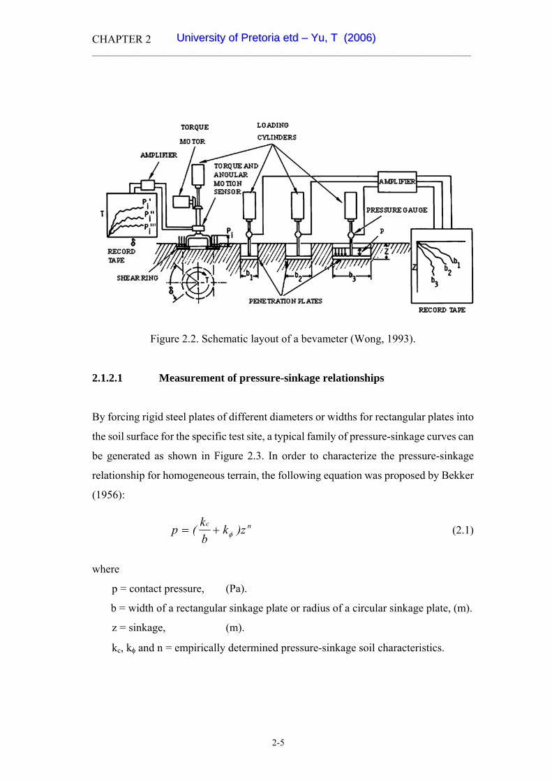
A soil-tyre numeric Ncs was proposed for cohesive-frictional soils by Wismer and Luth

(1973) as:

WdCIbN t

cs = (2.12)

The above mentioned three equations, especially equation (2.12), are the most

commonly used empirical relationships to predict traction performance for wheels. On

the bases of test results, mainly from soil bin tests in laboratories, the soil-tyre

numerics were correlated with the three traction performance parameters for tyres.

Among the parameters used in this equation, rolling resistance is a parameter often

correlated with the soil-tyre numerics.

Wismer and Luth (1973) developed the following generally used equations for not

highly compactible soils:

04.0N

2.1RW cs

r +==ρ (2.13)

)e1(75.0

WF

WrT SN3.0t

rg

cs−−===μ (2.14)

where

Rr = motion resistance, (N).

Ncs = wheel numeric, (CIbd/W).

2-17


CHAPTER 2 _________________________________________________________________________________

T = applied torque, (Nm).

rr = rolling radius based on a zero condition when net traction is zero at zero

slip on a hard surface, (m).

Ft = gross tractive force, (N).

W = vertical load, (N).

ρ = motion resistance ratio.

μg = gross traction coefficient.

For the determination of rr in the above equation, the slip is defined as:

(2.14a) %100)

rV1(i ×−=ω

where

V = velocity of the wheel centre, (m/s).

r = radius of the wheel, (m).

ω = angular velocity, (rad/s).

Thus, the wheel pull coefficient or traction coefficient μ was calculated from:

ρμμ −=−

= grt

WRF

(2.15)

For its simplicity and as only one parameter needed to be measured, the above

described empirical method based on cone index used by many users to evaluate

wheeled tractors under some given conditions. However, as pointed out by Wong

(1989), the original concept of using the simple measurement of cone index is limited

by the lack of information for the terrain conditions. The application is also strictly

limited to cases which are similar to the conditions under which the original tests were

undertaken. The exact range of soil conditions for which soil numerics are applicable

also remains to be determined. This method should therefore be used with caution if

the tyre or conditions differ from those under which the data were collected.

2-18


CHAPTER 2 _________________________________________________________________________________

2.2.2 Analytical methods for traction performance modelling

Based on the parameters measured by the bevameter technique, Bekker originally

developed one of the best known and most commonly used analytical methods - also

known as a semi-empirical method for traction (Bekker, 1956, 1960, 1969; Wong,

1989, 1993). The principle of this analytical method was based on the assumptions that

the vertical deformation in the soil under load was analogous to the soil deformation

under a sinkage plate and that the shear deformation of the soil under a traction device

was similar to the shear action performed by a rectangular or torsional shear device.

The motion resistance of the running gear on a soft soil surface was predicted by

assuming that the resistance was mainly caused by compacting the soil and the energy

dissipated in forming a rut in the soil below the running gear. The total tractive effort

was predicted by integrating the horizontal component of shear stress beneath the

running gear in the direction of travel.

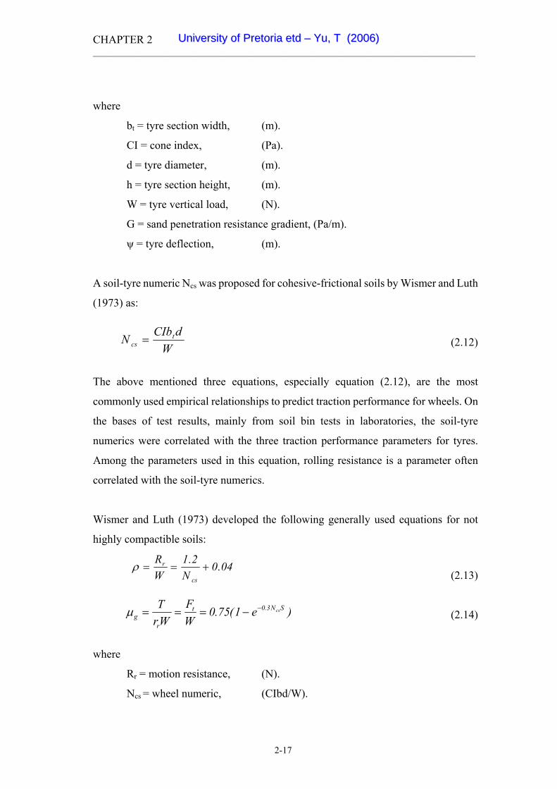
In the basic model proposed by Bekker (1956), a towed rigid wheel was analyzed

based on the configuration of the contact surface as shown in Figure 2.9. For this

simplified model, the motion resistance resulting from soil compaction was predicted

as:

∫ +=

rZ

0

ncwc dzz)k

bk(bR φ

)1n2/()1n()1n2/(1wc

)1n2/()2n2(

)1n2/()2n2(

D)kbk)(1n()n3()W3(

+++++

++

++−=

φ (2.16)

where

Rc = motion resistance, (N).

Zr = depth of the rut, (m).

bw = width of the wheel, (m).

W = wheel load, (N).

D = diameter of the wheel, (m).

kc, kφ and n = empirically determined pressure-sinkage soil characteristics.

2-19


CHAPTER 2 _________________________________________________________________________________

Figure 2.9. Simplified rigid wheel-soil interaction model by Bekker (1956).

This generalized equation is valid for moderate sinkage (i.e., z0≤D/6) for any rigid

wheel or highly inflated tyre with minimal deflection in homogeneous soft soils of any

type. It is more accurate for larger wheel diameters and limited sinkage in soft soil.

The sinkage of such a wheel z0 is also determined from the following equation (Bekker,

1956):

1n22

wc0 D)kbk)(n3(

W3z+

⎥⎥⎦

⎤

⎢⎢⎣

⎡

+−=

φ

(2.17)

where

z0 = sinkage of the wheel, (m).

bw = width of the wheel, (m).

The rest of the symbols are as defined in equation (2.16).

For a pneumatic tyre, when the terrain is firm and the inflation pressure is sufficiently

low, significant tyre deformation occurs (Figure 2.10). The sinkage of the tyre z0 in

this case can be determined by applying the following equation together with Bekker’s

sinkage equation:

n/1

wc

cti0 k)b/k(

ppz ⎟

⎟⎠

⎞⎜⎜⎝

⎛

++

=φ

(2.18)

2-20


CHAPTER 2 _________________________________________________________________________________

2-21

)kb/k)(1n()pp(bRwc

n/)1n(ctiw

cφ++

+=

+

Figure 2.10. Deformation of a pneumatic tyre in different operating modes

(Wong, 1989).

Under these circumstances, the motion resistance is given by:

(2.19)

where Rc

pti = inflation pressure, (Pa).

pc = pressure due to the stiffness of the carcass, (Pa).

As proposed by Wong & Reece (1967), the analysis for the shear displacement

developed along the contact area of a rigid wheel based on the analysis of the slip

velocity Vj is shown in Figure 2.11 and is described by:

]cos)i1(1[r V j θω −−= (2.20)

where

i = slip of the wheel as defined in equation (2.14a), (%).

r = wheel radius, (m).

ω = angular velocity of the wheel, (rad/s).

It is shown that the slip velocity for a rigid wheel varies with the angle θ and slip i.


CHAPTER 2 _________________________________________________________________________________

Figure 2.11. Analysis of shear displacement under a wheel (Wong, 1993).

The shear displacement along the interface is given by:

)]sin)(sini1()[(r

d]cos)i1(1[rdtVj

00

t

0 0j

0

θθθθωθθω

θ

−−−−=

−−== ∫ ∫(2.21)

where θ0 is the entrance angle of the wheel.

By applying the relationship of shear stress and shear displacement, as proposed by

Janosi and Hanamoto (1961), the shear stress can be described as:

]1][tan)([

)1](tan)([)()]sin)(sin1()[/(

/

00 θθθθφθ

φθθτ−−−−−−+=

−+=iKr

Kj

epc

epc(2.22)

By integrating the horizontal component of the stresses in the direction of travel over

the entire contact area, the total tractive effort Ft can be determined:

θdθcosτ(θ)F 0θ

0t ∫= (2.23)

To take into consideration the effect of shear stress on the vertical load and the effect

of normal stress on the horizontal force, the equations for predicting the vertical load

2-22


CHAPTER 2 _________________________________________________________________________________

2-23

(2.25)

a

pneum rati

sues for a wheel also include the distribution of normal and shear stress, and the

LLING FOR TRACKED VEHICLES

.3.1 Empirical methods for traction performance modelling

mpirical methods are still playing an important role for the evaluation of the

y based on cone

enetrometer values as originally developed by WES (Rula and Nuttall, 1971). They

ne of the most popular analytical methods for the performance of a track system was

sumption that the

ack in contact with the terrain is similar to a rigid footing. By using Bekker’s

⎥⎦⎤

⎢⎣⎡ −= ∫ ∫

0 0

0 0wh dsin)(pdcos)(rbFθ θ

θθθθθθτ

and drawbar pull for a rigid wheel are given by equations (2.24) and (2.25) (Wong,

1993) respectively.

For vertical load,

⎥⎦⎤

⎢⎣⎡ += ∫ ∫

0 0

0 0w dsin)(dcos)(prbWθ θ

θθθτθθθ (2.24)

For available pull,

Generally speaking, the methods for predicting the tractive performance for

on. Other key atic tyre are mainly dependent on the individual mode of ope

is

profile of the contact patch.

2.3 TRACTION MODE

2

E

performance of tracked vehicles. The empirical methods are mainl

p

follow similar methods used for the wheeled vehicles reviewed in the previous section.

2.3.2 Analytical methods for traction performance modelling

O

originally developed by Bekker (1956, 1960, 1969) based on the as

tr


CHAPTER 2 _________________________________________________________________________________

1/n

c

n/1

ct k)b/k(

W/bLk)b/k(

pz⎥⎥⎦

⎤

⎢⎢⎣

⎡

+=

⎥⎥⎦

⎤

⎢⎢⎣

⎡

+=

φφ

pressure-sinkage equation (2.1), for a rigid, relatively smooth, uniformly loaded track,

as shown in Figure 2.12, the track sinkage zt is given by:

(2.26)

n/)n(

n/c LW

)kb/k)(n(R

1

111 +

⎟⎠⎞

⎜⎝⎛

++=

The motion resistance of the track due to soil compaction Rc is

(2.27)

ong, 1989).

If the contact pressure is uniformly distributed and the shear stress-shear displacement

has a si rt of a

ack with contact area of A can be determined from:

(2.28)

:

c φ

Figure 2.12. Simplified model for track-soil interaction (W

mple exponential relationship as shown in equation (2.6), the tractive effo

tr

⎥⎦⎤

⎣)

iLK

⎢⎡ −−+=

−+=

−

−∫

e1(K1)tanWAc(

dx)e1)(tanbLWc(bF

/iL

K/ixL

0t

φ

φ

2-24


CHAPTER 2 _________________________________________________________________________________

Using the maximum shear strength τmax defined by equation (2.8), the max

active effort Ftmax is therefore determined as:

(2.29)

aximum pull Fhmax in horizontal direction are

expressed by:

(2.30)

(2.31)

y the theoretical

ssumption, Wills (1963) used a specially designed cantilever-type track link

imum

tr

φφ

τ

tanWAc ]tanpc[A

maxmaxt

+=+=

AF =

Thus the available pull Fh and the m

cth RFF −=n/)1n(

n/1c

K/iL

LW

)kb/k)(1n(1)e1(

iLK1)tanWAc(

+− ⎟

⎠⎞

⎜⎝⎛

++−⎥⎦

⎤⎢⎣⎡ −−+=

φ

φ

and

n/)1n(

n/1c

cmaxtmaxh

LW

)kb/k)(1n(1)tanWAc(

RFF+

⎟⎠⎞

⎜⎝⎛

++−+=

−=

φ

φ

Practically, the distribution of normal stress on the track-terrain interface plays an

important role for predicting the performance. In order to verif

a

dynamometer to determine the distribution of normal pressure under a uniformly

loaded rigid track by measuring the vertical and the horizontal forces between a track

link and a track plate. The magnitude and distribution of horizontal shear force

developed under the track were also measured. The effects of other different values of

normal stress distribution (Figure 2.13) on tractive efforts were also investigated by

Wills (1963).

2-25


CHAPTER 2 _________________________________________________________________________________

⎟⎟⎠

⎞⎜⎜⎝

⎛+=

Lxn2

cos1bLWp pπ

(2.32)

Figure 2.13. Various patterns of idealized contact pressure distribution under a track

(Wills, 1963).

It proved that the normal stress distribution beneath a rigid track influenced the

development of the tractive effort. In the case as shown in Figure 2.13(b), the normal

ressure p has a multi-peak sinusoidal distribution expressed by:

where n is the number of periods as shown in Figure 2.13. In a frictional soil with c=0,

the s contact lengt

(2.34)

p

p

hear stress developed along the h is expressed by:

(2.33)

)e1(

Lxn2

cos1tanbLW K/ixp −−⎟⎟

⎠

⎞⎜⎜⎝

⎛+=

πφτ

and the tractive effort is calculated as:

)1e(K)1e(K1Wtan

dx)e1(x

22222

K/iLK/iL

K/ix

⎥⎥⎤

⎢⎢⎡

+−

+−+=

−⎟⎟⎠

⎞

⎝−

−

−

πφ

π

Li/Kn41(iLiL

Ln2

cos1tanbLWbF

L

0

pt ⎜⎜

⎛+= ∫ φ

p ⎦⎣

2-26


CHAPTER 2 _________________________________________________________________________________

( )

eKiLe1

iLK21tanW

K/iLK/iL2

K/iL

⎥⎥⎦

⎤

⎢⎢⎣

⎡⎟⎠⎞

⎜⎝⎛ −−⎟

⎠⎞

⎜⎝⎛−−

⎥⎦⎤

−−φ

The tractive effort of a track with other contact pressure distribution p

lso predicted in a similar way. In the case of (c) (Figure 2.13), the pressure increases

(2.35)

rear to front, r

=2[W/(bL)](l-x)/L) as shown in Figure 2.13(d), the tractive effort of a track in

(2.36)

In the case of a sinusoidal distribution with maximum pressure at the center and zero

pressure at the front and rear end (p=(W/bL)(π/2)sin(πx/L), as in Figure 2.13(d)), the

tractive effort in a frictional soil is determined by:

rt with slip of a track with various

pes o entioned above (Wills, 1963). It

distribution has a noticeable effect on the

evelopment of tractive effort, particularly at low values of slip when the tractor is

atterns can be

a

linearly from front to rear p=2[W/(bL)](x/L), and the tractive effort of a track in

frictional soil is given by:

eKiLe1

iLK K/iLK/iL

⎥⎥⎦

⎤

⎢⎣⎟⎠⎞

⎜⎝⎛ −−⎟

⎠⎞

⎜⎝⎛ −−21tanWF

2

t ⎢⎡

−= φ

epresented by In the case of a contact pressure increasing linearly from

p

e1iLK1tanW2Ft ⎢⎣

⎡ −−= −φ

frictional soil is calculated from:

(2.37)

Figure 2.14 shows the variation of the tractive effo

ty f contact pressure distribution on sand, as m

can be seen that the contact pressure

d

usually operated. In this point of view, the bottom one of the pressure distribution

patterns as shown in the figure is most preferred for larger value of drawbar pull at

lower value of slip. In fact, the distribution of normal pressure and shear stress are

among the most important issues in the analytical models based on Bekker’s method.

⎥⎦

⎤⎢⎣

⎡+

+−=

)K/Li1(21e1tanWF 2222t π

φ− K/ilL

2-27


CHAPTER 2 _________________________________________________________________________________

Figure 2.14. Effect of contact pressure distribution on the tractive perform

track in sand (Wills, 1963).

ance of a

he experiments performed and the results obtained by Wills (1963) in the laboratory

ith full size rigid tracks are important because in these experiments both the vertical

a

However, due to the practica ansducers onto a track, little

effort has since been made to measure the normal and horizontal forces simultaneously

sumed to be

quivalent to a flexible belt and the assumed track-road wheel system travelling on a

T

w

nd the horizontal forces acting on a track link were measured simultaneously.

l difficulties to mount force tr

on the track. Other experiments aimed at the determination of the pressure distribution

under tracks were only restricted to the measurement of normal stresses.

Wong (1989, 1993) developed a model based on the analysis of track-terrain

interaction to predict the performance of the traditional steel track. In Wong’s model,

the contact pressure distribution was predicted by determining the shape of the

deflected track in contact with the terrain. In the analysis, the track is as

e

deformable terrain under steady-state conditions is shown in Figure 2.15. The

magnitude of the slip velocity Vj of a point P on a flexible track is expressed by:

(2.38) ]i)cos-(1-[1r i)cos-(1r-r

VVV tj

αωαωω

α

==

−= cos

2-28


CHAPTER 2 _________________________________________________________________________________

Figure 2.15. Deform odel

The shear displacement j along the track-terrain interface for contact length is given

y:

(2.39)

shear y:

(2.40)

here p(x) is the contact pressure on the track and is a function of x.

this tion resistance Re is given

by

(2.41)

ation of the interaction surface used in Wong’s m

(Wong, 1993).

b

i)x-(1-

i1(1[r 0

t

l

l

=

−−= ∫ ω

dt)]i1(1[rj0

−−= ∫ ω

rd)] l

ω

The stress distribution is expressed b

⎭⎩ ⎦⎣ ⎠⎝

w

In model, for a vehicle with two tracks, the external mo

⎬⎫

⎨⎧

⎥⎤

⎢⎡

⎟⎞

⎜⎛ −−

−−+=K

x)i1(exp1]tan)x(pc[)x( lφτ

0∫=t

e dsinpb2Rl

lα

2-29


CHAPTER 2 _________________________________________________________________________________

And the tractive effort Ft for a vehicle with two tracks is given by:

(2.42)

Wong’s model, the response to repetitive loading was also included in the analysis.

ween the measured and

predicted n v

corded.

was mentioned by Wong (1993) that for a track with rubber pads, the part of the

er pads in contact with the terrain, and the characteristics of rubber-terrain

ictional slip. However, there was no further description given in this respect.

itially, the idea of rubber tracks was proposed in the early 1970’s. The first type was

pneumatic rubber track tested by Taylor and Burt (1973). The pneumatic rubber

stretching wheels fixed to a frame. In their study, the traction performance and soil

ompaction was compared for a steel track, a pneumatic rubber track and a pneumatic

ll

dcosb2F t

∫= ατ0t

In

According to the reported results, a close agreement bet

alues as well as drawbar performance was contact pressure distributio

re

It

tractive effort generated by rubber-terrain interaction could be predicted by taking into

consideration the portion of the vehicle weight supported by the rubber pads, the area

of the rubb

fr

2.4 DEVELOPMENT OF AND TRACTION CHARACTERISTICS FOR

RUBBER TRACKS

In

a

track consisted of a circular shaped, and nylon reinforced flexible tyre, mounted over

c

tyre in a soil tank. The tractive efficiencies for various soil types ranged from 80% to

85% for both the steel and the pneumatic rubber tracks and from 55% to 65% for the

pneumatic tyre. Maximum tractive efficiencies occurred at less than 10% slip for the

tracks and between 15% and 25% for the tyre. In general, both the steel and pneumatic

tracks had comparable traction performance characteristics. However, the

performance of both tracks was much higher than that for a pneumatic tyre.

2-30


CHAPTER 2 _________________________________________________________________________________

Evans and Gove (1986) reported the test results comparing the tractive performance

and soil compaction for a rubber belt track and a four-wheel drive tractor. The tests

were conducted in tilled soil and firm soil and proved that the rubber belt tractor, in

comparison to the four-wheel drive tractor, developed higher tractive efficiencies at a

ecified pull ratio and generated an equivalent drawbar pull at lower slip levels. The

tyre on a

ngle wheel tester. The results proved that the rubber track produced about 25% more

disked

ats stubble, plowed oats stubble, and maize stubble. The tractive performance was

sp

maximum tractive efficiency in tilled and firm soil was 85% and 90% for the rubber

belt tractor and 70% and 85% for the four-wheel drive tractor. The reported results for

soil compaction tests conducted in the tilled soil showed that the rubber belt tractor

and the four-wheel drive tractor caused similar increases in cone penetration resistance

as they had equal mass. However, the measurement of subsoil pressure proved that at

the same depth, peak subsoil vertical stresses were twice as high for the four-wheel

drive tractor as for the rubber belt tractor. The rubber track also depicted a more

uniformly distributed contact pressure under the track than for the wheel.

Culshaw (1988) reported about two experiments in which the tractive performance of

rubber tracks were compared to that of tractor drive tyres. The first experiment was a

comparison between a friction drive rubber track and a conventional radial type tractor

tyre. The tests were conducted by alternatively mounting the track and the

si

drawbar pull than the tyre. The second experiment was a comparison between a small

dumping truck running on rubber tracks and a conventional two-wheel drive tractor

with a similar mass. It was proved that the truck produced twice the pull of the wheeled

tractor with similar tractive efficiencies and caused less rutting on a soft soil.

Esch, Bashford, Von Bargen and Ekström (1990) reported a comprehensive traction

performance comparison between a rubber belt track tractor and a four-wheel drive

tractor equipped with dual wheels, having comparable power and mass. The drawbar

tests were performed on four ground surface conditions: untilled oats stubble,

o

compared based on relationships of dynamic traction ratio to slip, tractive efficiency to

slip and tractive efficiency to dynamic traction ratio. It showed that the rubber belt

2-31


CHAPTER 2 _________________________________________________________________________________

track offered small advantages over the four-wheel drive tractor on firm surface but

significant advantages under soft surface conditions.

In the research reported by Okello et al (1994), it was found that the rubber tracks had

higher rolling resistance than the tractor driving wheel tyre apparently due to the

internal power losses in the track unit. Accordingly, the tractive efficiencies of the

bber tracks were lower than that of the tyre because of the higher rolling resistance

2.16), were described for predicting the tractive performance. The

ontact pressure at each point on the ground contact surface was calculated from the

(2.43)

:

(2.44)

nd

∫ +L

dxpb0

)sincos( βτβ

∫=0r dxsinpbR β

dx)sinp β−

ru

for the track.

Dwyer et al (1993) reviewed the research on rubber tracks at the Silsoe Research

Institute. Two mathematical models, namely an infinitely stiff and infinitely flexible

track (Figure

c

pressure-sinkage relationship in equation (2.1). The shear stress-shear displacement

relationship in equation (2.6) was applied to predict the tangential stress. The

equations of equilibrium were established by using the track deformation assumptions

for two extreme flexibility situations. The equilibrium equations for the infinitely stiff

model are as follow:

In the vertical direction:

=W

In the horizontal direction

L

a

cos(bFL

0t βτ∫= (2.45)

2-32


CHAPTER 2 _________________________________________________________________________________

odels

ith the infinitely stiff assumption, the solution was independent of the diameter or

spacing o ctangular

plate. With the infinitely flexi t behaved like a multi-wheel

ehicle, as if there was no track at all, and the performance depended entirely on the

il

haracterization parameters obtained by applying shear and sinkage tests based on the

Figure 2.16. The infinitely stiff and the infinitely flexible m

by Dwyer et al. (1993).

W

f the ground rollers and the ground contact area was a flat and re

ble model, the track uni

v

number and diameter of the ground rollers. The results of the field tests with the

experimental track unit on a single-wheel tester proved that the tractive performance

of the rubber track was over-predicted by the infinitely stiff model and considerably

under-predicted by the infinitely flexible model. The method, based on Wong’s

procedure, was used in the analysis. They determined that the profile of ground contact

surface and thus the stress distribution was the major factor causing the difference.

A model was developed by Okello et al (1998) to study the traction performance and

ground pressure distribution of a rubber track unit on soft agricultural soils. By closely

following Wong’s method of steel tracks, the model made use of relevant so

c

2-33


CHAPTER 2 _________________________________________________________________________________

bevameter technique. The effect of repetitive loading was also taken into consideration

by the procedure suggested by Wong (1989). For their research a rubber track unit was

mounted on a structure similar to the one for a traditional steel track. The theoretical

model was validated against the experimental results by attaching the rubber track unit

to the rear of a single-wheel tester. For two of the four soil conditions tested, the results

from the theoretical prediction and the experimental data were compared and showed

close agreement with a maximum difference of only 7.5%. For other two soil

conditions, the predicted results were not provided for the reason of failed soil shear

tests.

In recent years, the rubber tracks became more popular for their combined advantages

when compared to conventional steel tracks and the wheels, as summarized in Chapter

1. The rubber tracks are currently mainly used on agricultural tractors and some

onstruction machinery. However, they are also used on combines.

l features for the

hallenger Series were reported in the relevant ASAE lectures (Caterpillar Inc., 1995).

ay lead to slipping of the rubber belt, but with minimal belt damage. However, a

c

After the development over a decade, the Challenger tractor series equipped with

rubber belt tracks from Caterpillar became the major rubber track crawler tractors

available on the market. The historical development and the technica

C

A friction drive is utilized to transmit the power from the sprocket to the rubber belt

tracks and the rubber tracks have lugs in contact with soil to generate the thrust effort.

According to the design principle, if the track tension is set higher than the maximum

traction effort developed by the track, slip will not occur between the track and the

driving wheel and the efficiency will not be reduced. Overloading of friction drives

m

combination friction/positive drive unit leads to a longer service life for the rubber belt

and positive safe transmission of driving power (Dudzinksi & Ketting, 1996). Besides

the success of the Challenger crawler tractors, other types of rubber tracks are also

being pursued for improved tractor construction. It is still too early to reach a

conclusion whether the friction driven tracks used on the Challenger series is superior

to the positive drive rubber track with sprocket as developed by Bridgestone.

2-34


CHAPTER 2 _________________________________________________________________________________

As can be seen from the above review, the previous research was mainly concentrating

on the comparison of performance for the rubber tracks and conventional traction

devices. Further research needs to be done on the prediction of performance and

traction modelling to develop a better understanding of the traction mechanism and to

ENTIAL STRESSES BELOW A TRACK

.5.1 Track link dynamometer by Wills (1963)

In orde sure distributions, Wills

esigned and built a cantilevered dynamometer beam as shown in Figure 2.17. By the

a ion and magnitude of the contact

ressure and horizontal shear force below a steel track was measured simultaneously.

guide further improvement of the design for rubber tracks if they are to be utilized on a

larger scale.

2.5 MEASUREMENT OF THE DISTRIBUTION OF CONTACT AND

TANG

2

r to verify the assumptions of different contact pres

d

applic tion of strain gauge transducers, the distribut

p

The results in sand for different distribution types were also compared.

The results from Will’s research work are currently still cited by many researchers.

2-35


CHAPTER 2 _________________________________________________________________________________

Figure 2.17. Track link dynamometer by W

Applications of extended octagonal

ills (1963).

2.5.2 ring transducers for measuring two

perpendicular forces

he principle of the circular ring is used as the basis for the measurement of two

Figure 2.18, with the circular ring and the properly arranged strain gauge bridge

ircuits, it is possible to measure the two orthogonal forces P and F independently. The

T

orthogonal forces in its plane of symmetry (Lowen & Cook, 1956). As shown in

c

octagonal form of the ring (Figure 2.18, top right) results in greater stability for the

measurement of both forces. The most useful form is obtained by extending the

octagonal ring by 2Lo (Figure 2.18, bottom). The extended octagonal ring ensures

sufficient stability for most practical applications. It also minimizes the bending

effects and maintains as nearly as practicable the condition of zero rotation of the top

surface. The extended octagonal ring transducers have been used in agricultural

engineering by many researchers (Godwin, 1975; O’Dogherty, 1975; Thakur &

Godwin, 1988; Girma, 1989).

2-36


CHAPTER 2 _________________________________________________________________________________

In Figure 2.18, the strain and stress at the inside and the outside surfaces of the ring

due to the forces P and F are zero at θ=nodal angles, φP and φF respectively. With the

strain gauges mounted in these positions and connected into the Wheatstone bridge

ircuits, the gauges 1-4 will measure the force F, eliminating the influence of the force

(2.47)

n ( ), kP is the constant for P, in practice ranging from 1.50 to 1.78 with a

mean value o (

.02 with mean value of 1.80, while φP is the nodal angle at which stress, due to force

is zero. The value of φP ranges from 34° to 50° according to various researchers. For

c

P, while the gauges 5-8 will measure the force P, eliminating force F.

Although no exact solutions exists for the strain of an extended octagonal ring, the

following approximate equations were suggested by O’Dogherty (1996) to predict the

value of the strain caused by force P and F respectively:

Force P:

(2.46)

Force F:

2oo

oP90 tEb

Prk=oε

2oo

oF

tEbFrk

f=φε

In equatio 462.

2.47), kF is the constant for F, ranging from 1.66 to f 1.70. In equation

2

P

a specific application φP rather needs to be determined by calibration. E is the modulus

of elasticity of the ring material.

2-37


CHAPTER 2 _________________________________________________________________________________

Figure 2.18. The Extended octagonal ring transducer (Godwin, 1975)

2.6 DEVELOPMENT OF THE PROTOTYPE TRACTION SYSTEM

raction

system val track), was developed and

ounted on a prototype tractor based on a new Allis Chalmers four-wheel drive tractor

f a very large diameter wheel (Figure 2.19). This was achieved by

BASED ON SOIL-RUBBER FRICTION

A rubber-surfaced and friction-based track system, initially named a Bi-pole t

(two pole wheels used at the ends of the o

m

(Barnard, 1989).

As described by du Plessis (1996), the prototype traction concept was invented to have

the terrain effect o

2-38


CHAPTER 2 _________________________________________________________________________________

constructing an articulated beam type track which resists inward articulation, but

antly reduced steering resistance and damage to the ground surface when

eered (Figure 2.19). It offers the additional advantage that the individual track

Figure 2.19. The construction concept of the prototype track to achieve the effect of a

very large diameter wheel.

The initial field performance ed with this prototype track

ystem proved that the maximum drawbar pull and power on a concrete surface at a

hosen speed was notably higher than for the equivalent four-wheel drive tractor (du

allows outward articulation carried by two pairs of pneumatic wheels (N) for each

track.

By using the middle wheels (M) on the track, the tractor was also expected to have

signific

st

elements can easily be replaced at low cost when compared to damaged rubber belt

tracks. As the prototype track represents an alternative principle to achieve the same

characteristics as the rubber belt tracks, it has the potential to be competitive to other

similar mechanisms.

M

NN

GroundGround

tests for the tractor equipp

s

c

2-39


CHAPTER 2 _________________________________________________________________________________

Plessis, 1996). Other performance parameters were also enhanced by the prototype

tracks as summarized in the report (Barnard, 1989).

2.7 JUSTIFICATION FOR CONDUCTING THIS STUDY

he literature review indicates that extensive information has been published on the

roaches pioneered

y Bekker. However, there is no idealized universal approach to adequately predict

5). Extensive efforts need to be made for

proving the design principle of rubber tracks. It is obvious that any research and

rties for analytical traction modelling.

l as the tangential stress, will be

derived.

e years ago. The extended octagonal ring transducers are suitable to

measure the vertical and the horizontal forces on the track elements.

T

subject of vehicle-terrain interaction, especially the analytical app

b

and evaluate the new traction device. There is also very limited literature available for

in depth research about rubber tracks.

The utilization of the rubber tracks is still in the early and rapidly developing stage

(Evans and Gove, 1986. ASAE, 199

im

study work on this newly developed traction device would be beneficial and valuable

to the future design of the traction device.

The reviewed literature has led to the following proposed approach for this study

undertaken:

The bevameter technique is a realistic approach to characterize the soil

prope

Based on the previous study, an analytical model to predict the contact

pressure distribution below the track, as wel

The measurement of vertical contact pressure and the tangential stress was

done som

2-40


CHAPTER 2 _________________________________________________________________________________

The shape of the terrain contact surface of the prototype track is different from

that of previous traction devices. Thus the rationale of such a traction system

needs to be evaluated for further improvement.

From Neal’s research (1966), it was indicated that in sandy soils, where the

values of rubber-soil friction coefficient were similar to the values of the

coefficient of soil internal shear resistance, the performance of a friction-based

traction device such as the prototype track in this research was expected to be

at low values of slip when the tractor was usually operated.

It was preferred to keep the pressure distribution in the pattern that the

el track system.

2.8

fter the above literature review, the specific objectives of this study were:

riate analytical model to predict the drawbar performance

for the prototype track based on the friction-shear principle between rubber

almost similar to that of shear-based traction device, i. e. the traditional steel

tracks or wheels.

According to the research by Wills (1963) as shown in Figure 2.14, the contact

pressure distribution had a noticeable effect on the development of tractive

effort, particularly

magnitude of the pressure at the rear end was maximum whilst at the front end

the pressure was close to zero.

The prototype track system designed by Barnard (1989) based on frictional

principle was expected to have comparable tractive performance to the

performance of a traditional ste

OBJECTIVES

A

to develop an approp

and soil on a soft terrain surface;

2-41


CHAPTER 2 _________________________________________________________________________________

to build the necessary measurement and instrumentation system to acquire the

distribution of the contact and the tangential stresses under the prototype track;

to measure the required soil and rubber characteristics necessary for traction

to undertake the field tests for validation of the data from the traction

to evaluate the effects of the design features of the prototype traction system on

to proof that the performance of a shear-based and a friction-based traction

he soil parameters required for the development of the analytical model were

obt e

Particularly, the characterization of the rubber-soil friction and shear were undertaken

y using a standard track element. A computerized data acquisition system was used to

The structure of the prototype track was modified to accommodate the

stallation of these transducers.

.

modelling;

modelling and the experiments under various soil conditions;

the tractive performance; and

mechanism is almost similar.

T

ain d by using the instrumented apparatus applying the bevameter technique.

b

record all the in situ test results for the soil characterization and the full size drawbar

tests.

The special transducers to measure the distribution of the contact pressure and the

friction-shear stress were built according to the principle of the extended octagonal

ring.

in

After the validation of the results from the field tests and the modelling, some design

features such as the frictional drive principle, the track tensioning and the function of

the middle wheels were evaluated

2-42


CHAPTER 2 _________________________________________________________________________________

Figure 2.20 shows the flow chart of the procedure by which the above objectives were

achieved.

Soilcharacbased o

terizationn bevameter

technique andrubber-soilfriction.

Development of the analyticalmodel based on rubber-soil

Parameters of theprototype crawlerwith rubber track

system

friction to predict thetractive performance of the

prototype track on soft terrainsurface

Validation andcomparison of themodel data andthe field test

results

Measurement of thedistribution

of the contact pressure andthe tangential stress

Measurement for fullsize drawbar pull tests

in the field undervarious soil conditions

Figure 2.20. Flow chart of the proposed research procedure.

Evaluation for thedesign features,conclusions andrecommendations

2-43


CHAPTER 3 _________________________________________________________________________________

CHAPTER III

CONSTRUCTION OF THE PROTOTYPE RUBBER-FRICTION TRACTION SYSTEM

3. 1 INTRODUCTION

The crawler tractor, equipped with the prototype rubber-friction track under

investigation was initially named “Di-Pole Tractor” by the inventor (Barnard, 1989).

It was based on a four-wheel drive Allis Chalmers 8070 tractor with a 141 kW

engine (du Plessis, 1996). Compared to the popularly used Caterpillar Challenger

tractors, the prototype crawler under investigation had a common feature, namely the

rubber contact surface with the terrain. However, the thrust generating rationale for

the prototype crawler was based on friction, whilst the Caterpillar Challengers was

based on soil shear. In addition to the advantages of the rubber contact surface with

the ground, the prototype track system also had as features:

• rubber-covered track elements, linked by five parallel cable loops forming each

of the two tracks as articulated walking beams;

• a friction drive between the pneumatic drive wheels and the track and between

the track and the terrain surface;

• track tension adjusted by horizontally mounted hydraulic cylinders on the track

suspension;

• a steering control system with automatic differential lock;

• two ground wheels at the centre of each track, applying a vertical force to ease

the steering operation;

• achieving pivot steering about its own vertical axis; and

• considerably reduced specific ground pressure for this prototype tractor in

comparison to a similar wheeled tractor.

3-1


CHAPTER 3 _________________________________________________________________________________

Some comparative performance test results between the Di-Pole and conventional

four-wheel drive tractors are given in Table 3.1.

Table 3.1 Comparative test results for the prototype Di-Pole and conventional Allis

Chalmers 8070 four-wheel drive tractor on sandy soil (Barnard, 1989).

Tractor Type

Tractor

speed

(km/h)

Drawbar

pull

(kN)

Implement

width

(tilled)

(m)

Cultivation

rate

(h/ha) (ha/h)

Diesel

consumption

(l/h) (l/ha)

Di-Pole

AC Conventional

6.5

6.5

39

31

2.45

1.94

0.63 1.59

0.79 1.26

37

29

23.38

22.95

Di-Pole

AC Conventional

5.5

5.5

55

43

4.12

3.22

0.44 2.27

0.56 1.77

41

31

18.11

17.51

Di-Pole

AC Conventional

4.25

4.25

74

55

10.10

7.51

0.23 4.29

0.31 3.19

41

32

9.55

10.03

Di-Pole

AC Conventional

3.2

3.2

105

62

16.24

9.59

0.19 5.20

0.32 3.07

41.5

29

7.98

9.45

The above test results proved that under comparable conditions, the modified crawler

with rubber-covered track elements had a much higher drawbar pull and working rate

when compared to the original conventional tractor using the same engine. With

higher drawbar pull, the engine for the modified crawler was better loaded with a

higher torque applied to the tracks and therefore, the total fuel consumption in liter

per hour was higher, but almost the same in liter per hectare. At lower speeds, the

slip losses probably influenced the total fuel consumption for the conventional four-

wheel drive tractor negatively, resulting in higher fuel consumption in liter per

hectare. Unfortunately, no values of slip versus pull were supplied in the report.

Although the comparison may scientifically be questionable, Barnard (1989)

intended a comparison under typical farm conditions.

3-2


CHAPTER 3 _________________________________________________________________________________

In this Chapter, the technical and constructional features of the prototype track, as

tested on the modified tractor, will be described.

3.2 THE PROTOTYPE TRACK

3.2.1 The fundamental construction and layout

As the basic component of the track, each track element has a steel base plate (B)

with a rubber pad (A) bonded to it (Figure 3.1).

(A) rubber pad to form track surface (B) steel base plate to carry rubber pad

(C) steel stud (D) steel plate carried by steel cables

(E) inner rubber pad to form inner friction surface

(E) replaceable inner rubber pad and its steel plate (F) steel loop cables

(G) rubber tyre

Figure 3.1. The fundamental components of the prototype track.

3-3


CHAPTER 3 _________________________________________________________________________________

In practice, it proved that the structure of the track element was robust enough as the

rubber pad never got detached during the durability tests. The steel base plates (D)

fixed to the track element by studs (C) are kept in position by five steel cable loops

(F). The inner rubber pad (E) is bonded to a thinner steel plate, and is linked by a bolt

through the holes to steel plate (D) and threaded into the centre of the steel column

(C). By rotating the column (C), the track element (A) together with (B) and the

rubber pad (E) can be separated from the base plate (D).

Figure 3.2 shows an individual rubber-covered track element removed from the track

assembly. As the track is composed of 101 individual track elements, instead of an

integral belt, as used by other rubber tracks, any track element can be replaced

individually within a reasonable breakdown time. The track therefore need not be

replaced as a complete unit when partially damaged.

Figure 3.2. The individual track element.

Figure 3.3 shows the side view of the tractor equipped with the track. Two double

rear wheels (Figure 3.3 (A)) with smooth pneumatic biasply tyres are fixed to the

rear drive shafts on each side to provide rear wheel propulsion by frictional contact

with the rubber-covered inner surface of the track. In comparison to the active drive,

this frictional drive automatically protects the mechanical system against overload.

Unfortunately, slipping losses may be caused by decreased track tension and

propulsion force when the tractive load is high or the frictional properties

deteriorates, caused by operational circumstances such as heat, water, soil or other

3-4


CHAPTER 3 _________________________________________________________________________________

foreign inclusions. It was found from the initial tests that the slip was increased by

low track tension.

To prevent damage at the interference by mud entering the friction surface, the

friction drive periphery of the prototype track is positioned 200mm above the ground

level. The height of the track elements and the rubber pad (Figure 3.3) lifts the

internal rubber frictional surface of the track well above ground level, making it less

susceptible to inclusion of foreign material like mud at the driving surface. This also

prevents a bulldozing effect occurring when steering.

(A) Rubber tyre (B) Centre ground wheel (C) Dividing flanges

(D) Swinging axle mounting (E) Hydraulic ram adjusting the track tension

(F) Locking device

Figure 3.3. Side view of the prototype track fitted to the tractor.

3-5


CHAPTER 3 _________________________________________________________________________________

3.2.2 The centre ground wheels

Hydraulically activated centre ground wheels (Figure 3.3 (B)), with solid rubber

tyres, can be lifted or pushed down when necessary. During steering, the centre

ground wheels are forced against the lower portion of the track so as to increase the

curvature of the track and thus decrease the contact area. Pivot steering is approached

by the two wheels on each side, fixed to a single axle. For sharp turns, when one

track was driven forwards and the other rearwards with the centre wheels pushed

down onto the tracks, tractor turned along in a circular path around the vertical axis

of the tractor with minimal damage to the soil surface.

Under normal operational conditions for straight line travel, the centre wheels (B)

may be moderately pushed down onto the track to help achieve a more evenly

distributed ground contact pressure. However, this was not the original design

purpose of the centre wheels.

3.2.3 Track mounting, tensioning and driving friction at interface

The tracks are carried by two vertically swinging axle mountings (Figure 3.3 (D))

pivoted around the original rear axle extensions with the cranks loaded by rubber

springs at the front. This facilitates the use of the original tractor T-frame for

mounting the two track assembly units on to the original frame of either side shaft,

without necessitating any changes to the existing drive system. Frictional propulsion

is generated by contact of the flat-treaded pneumatic tyres (Figure 3.3 (A)) with the

inner track elements consisting of compression–molded composite of a carboxylated

nitrite.

The track is laterally constrained by dividing flanges (Figure 3.3 (C)) at the centre of

the inner track surface fitting into the gap formed between the side walls of the two

pneumatic drive wheels and the two pneumatic tensioning wheels.

3-6


CHAPTER 3 _________________________________________________________________________________

By extending the centre distance between the driving wheels and the driven wheels

by means of permanently mounted hydraulic rams (Figure 3.3 (E)), the track tension

necessary for the driving friction can be set by applying the correct pressure to the

tension cylinders. The mechanical locking device (Figure 3.3 (F)) maintains the

tension during normal operation. However after several hours of use, it may lose grip

and must be retensioned. The frictional propulsion of the track is also assisted by the

deflection of the tyre side walls clamping the central dividing flanges (C) when the

tyre side walls are deflected outwards by the vertical load.

3.2.4 The beam effect

In order to achieve the so called “walking beam effect”, the track elements were

designed with dimensions A<B<C<D as shown in Figure 3.4. It was claimed to

function in a way that when a series of wedge-shaped track elements were linked by

the five close loop cables, an oval shape, as seen from side, was formed by the track.

The curvature of the upper and lower portions of the track is therefore obtained from

the slightly wedged shape of the track elements, extending outwards beyond the

inner peripheries of the steel cables. The lower free span of the track in contact with

the soil behaved like a compound beam, stressed by the mass of the tractor. The

radius of the ground contact arc depended on the load and according to the designer

varied between about 30 meters and infinity, but the claim was not proofed. The

elastic resistance of the straightened track was expected to provide a more uniform

pressure distribution underneath the track than for a conventional flexible rubber

track supported only by road wheels.

As reported by du Plessis (1996), the walking beam effect was reduced, probably due

to cable strain and wear on the contact surfaces between track elements. During tests

flat metal spacers were inserted between the track elements to restore the beam effect,

but they were soon damaged (Figure 3.4 (E)) and the beam effect was lost again.

3-7


CHAPTER 3 _________________________________________________________________________________

Figure 3.4. The wedge-shaped track elements to enable the beam effect.

3.3 THE DRIVE TRAIN, STEERING CONTROL AND AUTOMATIC

DIFFERENTIAL LOCK

The patented drivetrain featured with the automatic differential lock, the differential

steering system and the swing mounted track carriers constitute an important part of

the design. The schematic layout of the drive train of the tractor, equipped with the

prototype track, is shown in Figure 3.5 (du Plessis, 1996).

The control differential (S) consisted of nitride spur gears, driven by the input shafts

K1 and K2 (Figure 3.5a). The input ring gear (R) is mounted around a circular cage

(K) and a pair of half shafts (H1 and H2) with spur gears (R1 and R2) (Figure 3.5 b) at

their inner ends. Spur pinions (A) are provided as two identical pairs in a

diametrically opposite arrangement on a pitch circle about the half shafts H1 and H2.

The spur pinions (A) are meshed with the spur gears (R1 and R2) and with each other.

3-8


CHAPTER 3 _________________________________________________________________________________

Figure 3.5. The drive train and the differential lock.

In the control differential (S), the half shafts (K1) and (H1) are interconnected by spur

pinions (T1) and (T2) to accommodate the distance between the shafts. Spur gear (K3)

is fixed to the half shaft (K2) and spur pinion (Y) is fixed to the half shaft (H2) with

idler gear (T3) to form a gear train driving (K2) and (H2) in the same direction. With a

gear ratio of about 6:1 the shafts (H1 and H2) rotate in opposite directions at a speed

six times that of K1 and K2, thus reducing the shaft diameter and mass.

3-9


CHAPTER 3 _________________________________________________________________________________

For straight line travel the half shafts (K1) and (K2) rotate at the same speed and

direction and the spur pinion (A1) and (A2) in an opposite direction at equal but a

higher speed, but at zero torque. They do not orbit and the ring gear (R) is stationary.

The spur pinions are driven by (H1) and (H2), but are also interlocked as shown on

the end views and the differential is automatically locked.

When steering, the variable displacement hydraulic piston pump (E), and the motor

(M) drives the control differential via a worm gear (W) in a desired direction and

speed, corresponding to the steering angle. The force from the inside track is thus

transferred to the outside track via the control differential (S) and regeneration takes

place. One track may even move forward and the other rearwards.

With an asymmetrical resistance, one track would tend to slow down and the other to

speed up, due to differential operation. This unequal torque tends to rotate the

differential (S), the ring gear (R), gear (W) and the motor (M). With a closed

hydraulic valve, or a worm gear (W) with a speed ratio of at least 6:1, the control

differential is locked and unstable steering action is thus prevented.

For straight travel, the spur pinions (A) spin at a high speed and conventional

differentials with bevel gears are not suitable. Contrary to the standard cantilever

arrangement, the spur pinions (A) are also supported on either side by bearings (L3

and L4). Large diameter thin-walled hollow shafts (H1 and H2) are used to enhance

the load carrying capacity and resilience with minimal inertia.

The design features as explained enable regeneration and replace complex devices

such as a null shaft.

3-10


CHAPTER 3 _________________________________________________________________________________

3.4 DIMENSIONS OF THE PROTOTYPE TRACK

Based on the original design, the relevant dimensions of the track are shown in

Figure 3.6. The distance between the front and the rear axles can be adjusted up to

2000 mm at maximum by hydraulic cylinder (E) as shown in Figure 3.3.

1800-2000

Ø1060 Ø1060

500

Ø450

200

Figure 3.6. The dimensions of the prototype track.

3.5 PRELIMINARY TESTS AND ASSESMENT OF TRACTIVE PERFORMANCE

Tests carried out to evaluate the handling and performance characteristics of the

prototype track system were reported by du Plessis (1996). The test results for this

field performance evaluation are shown in Table 3.2. The engine for the wheeled

3-11


CHAPTER 3 _________________________________________________________________________________

tractor was used and the crawler had a new engine, thus the dynamometer measured

power for the two engines were slightly different.

Table 3.2. The comparative test results for the prototype crawler and a four-wheel

drive tractor (du Plessis, 1996).

Type

Conventional four-wheel

drive tractor (used Allis

Chalmers 8070)

Di-Pole crawler

(Based on new Allis

Chalmers 8070

tractor)

Engine power tests

Maximum engine power (kW) Maximum torque (Nm)

132kW@2400rpm 600Nm@1800rpm

141kW@2400rpm 645Nm@1800rpm

Test on a soft surface

Gear for maximum power Maximum drawbar power (kW) Drawbar pull (kN) Speed (km/h) Rolling resistance (kN) Wheel or track/soil slip (%) Slip between drive wheels and track (%)

4 Low 58 31 6.8 9 Front 19.0, rear 21 -

4 Low 63 53 4.3 14 5.9 9.4

Test on a concrete surface

Gear Maximum drawbar power (kW) Drawbar pull (kN) Speed (km/h) Rolling resistance (kN) Wheel or track/road slip (%) Slip between drive wheels and track (%)

4 Low 77 38 7.3 8 Front 4.7, rear 4.4 -

4 Low 79 55 5.2 9.5 1.0 3.4

The engine for the conventional four-wheel drive tractor was used whilst that for the

crawler was new, thus the difference in power existed. The results showed that on

both a concrete and a soft surface, most of the performance characteristics for the

prototype crawler were superior to that of the conventional four-wheel drive tractor

equipped with a similar specification, but used engine. Particularly for the test on a

soft surface, the slip of the crawler tractor was at 5.9% whilst the wheeled tractor at

20%. However, the rolling resistance for the crawler was higher than for the standard

3-12


CHAPTER 3 _________________________________________________________________________________

four-wheel drive tractor for both hard and soft surfaces. The friction between the

track and the drive wheels for the crawler was another factor which influenced the

performance of the crawler negatively. The distribution of the contact pressure as

observed was uneven and the beam effect, as was envisaged by the original design,

did not materialize (du Plessis, 1996).

3.6 SUMMARY AND REMARKS

Based on the description of the design and construction in this chapter, it is shown

that the prototype crawler featured with the friction-based track and the patented

drive train system is uniquely distinct from other wheeled tractors or crawlers

currently in use. Theoretical traction performance modelling had not been carried out

for such a tractor. The assessment of factors influencing the traction performance

would also be of interest. Therefore, the following conclusions were drawn:

• The rubber-rubber and rubber-terrain friction-based track played an important

role in distinguishing the prototype crawler from other tractors.

• The drive train including the automatic differential lock performed well.

• More specialized tests needed to be conducted if the tractive performance of

the track was to be evaluated or validated by modelling.

• The walking beam effect could be restored partly by means of inserting some

flat metal sheet spacers between track elements to restore the outer circular

length of the track. However, they were soon damaged and the beam effect

was lost again.

3-13


CHAPTER 4 _________________________________________________________________________________

CHAPTER IV

DEVELOPMENT OF THE TRACTION MODEL FOR THE PROTOTYPE TRACK

4.1. INTRODUCTION

Based on the literature review in Chapter 2, analytical methods of modeling were

preferred to other method for this research. For analytical methods fewer parameters

were needed to be measured with than methods such as the finite element analysis

(FEM). Analytical methods also offered closer simulation to the real tractive

phenomenon than the empirical approaches such as the methods based on cone index.

After years of research and assessment by researchers, analytical methods for soil

characterization and traction modelling based on the bevameter technique is still a

preferred technique. For its feasibility and simplicity, the approach based on

bevameter technique was therefore chosen for this research.

To develop the traction model by applying analytical methods based on the

bevameter technique, characteristics of the friction between the track and the terrain

surface, limited soil shear characteristics, and the pressure-sinkage relationship had

to be determined. The soil parameters and the distribution of the contact pressure

could be applied for the prediction of the tractive performance. By applying Bekker’s

analysis of motion resistance, mainly caused by soil compaction and the loss from

internal track friction, the total motion resistance could be predicted.

The distribution of the contact and tangential stresses relies mainly on the

deformation of the track and the terrain surface. When the bevameter technique was

applied to predict the distribution and magnitude of the ground contact pressure

under the track, the shape of the deflected track in contact with the terrain surface

4-1


CHAPTER 4 _________________________________________________________________________________

was of importance. A detailed analysis of the pressure distribution at the track–

terrain interface was made. For traction modelling the relationship between the

relevant vehicle parameters associated with the deformed track shape in contact with

the terrain and the soil characteristics was established.

4.2 CHARACTERIZATION OF RUBBER-SOIL FRICTION AND SOIL SHEAR WITH DISPLACEMENT

As reviewed and discussed in the preceding chapters, the thrust between the running

gear and the terrain surface, for a traditional tractive device, is usually developed by

the internal soil shearing action associated with relative slip. It is the rationale that

the prototype track generates tractive thrust mainly by friction between the smooth

rubber surface and the terrain surface whilst the soil-soil shear is minimal. The

characterization of the relationship for soil shear stress versus shear displacement,

and soil-rubber friction versus displacement was thus required for the proposed

modelling procedure.

When the shear action occurs in the soil, which is typical for a tractive device with

grousers moving over a soft terrain surface, the maximum shear stress τmax can be

described by the Mohr-Coulomb failure equation, i.e. equation 2.11.

The Mohr-Coulomb equation describes the shear strength of soil to soil, therefore it

is valid when used to simulate the shearing action of a tyre or track with lugs

penetrating into the soil. Shear action in the soil is caused by the moving lugs when

the running gear propels the vehicle. However, when the surface of the running gear

is smooth and the slip action apparently occurs at the soil contact surface, it is more

appropriate to describe the phenomenon as frictional. Thus it is better expressed by

applying another equation of similar form but with different parameters for the

maximum frictional stress τ fmax at the frictional contact surface as expressed by:

(4.1) δtanpc τ afmax +=

4-2


CHAPTER 4 _________________________________________________________________________________

where

ca = soil-rubber adhesion on the interacting surface, (Pa).

p = contact stress on the interacting surface, (Pa).

δ = angle of soil-rubber friction, (degrees).

From the preparatory field measurements in this research, the values of the soil shear

parameters obtained from steel shear grousers were different from the measured

friction-shear parameters obtained by using the rubber-coated track element as a

friction plate with a smooth rubber surface (Yu, 1996). It was also found that the

values of the coefficient of soil to rubber surface friction tan δ, and the internal

shearing resistance of the soil tan φ were very similar as shown in Table 4.1. The

adhesion between rubber and soil was less than the internal cohesion of the soil. This

was in accordance with values reported by Neal (1966) and Wills (1963). Therefore

the two cases of soil shear and rubber-soil friction must be considered differently for

traction modelling.

Table 4.1. Comparison of soil internal shear and soil-rubber friction parameters

(Yu, 1996).

Soil water

content (dry

basis), %

Internal

frictional angle

for soil shear

φ, degrees

Soil internal

cohesion c,

kPa

Soil-rubber

frictional angle

δ, degrees

Soil-rubber

adhesion ca,

kPa

10.9 33.9 1.62 29.4 1.55

21.6 31.1 2.59 29.9 2.69

35.3 30.9 3.34 28.7 2.49

The tractive thrust for the prototype track under investigation is generated by the

smooth rubber surface when the track, composed of individual track elements,

develops pull on soft terrain surface. For the interaction between the track element

and the soil surface, the soil-rubber frictional action is dominant, rather than the

4-3


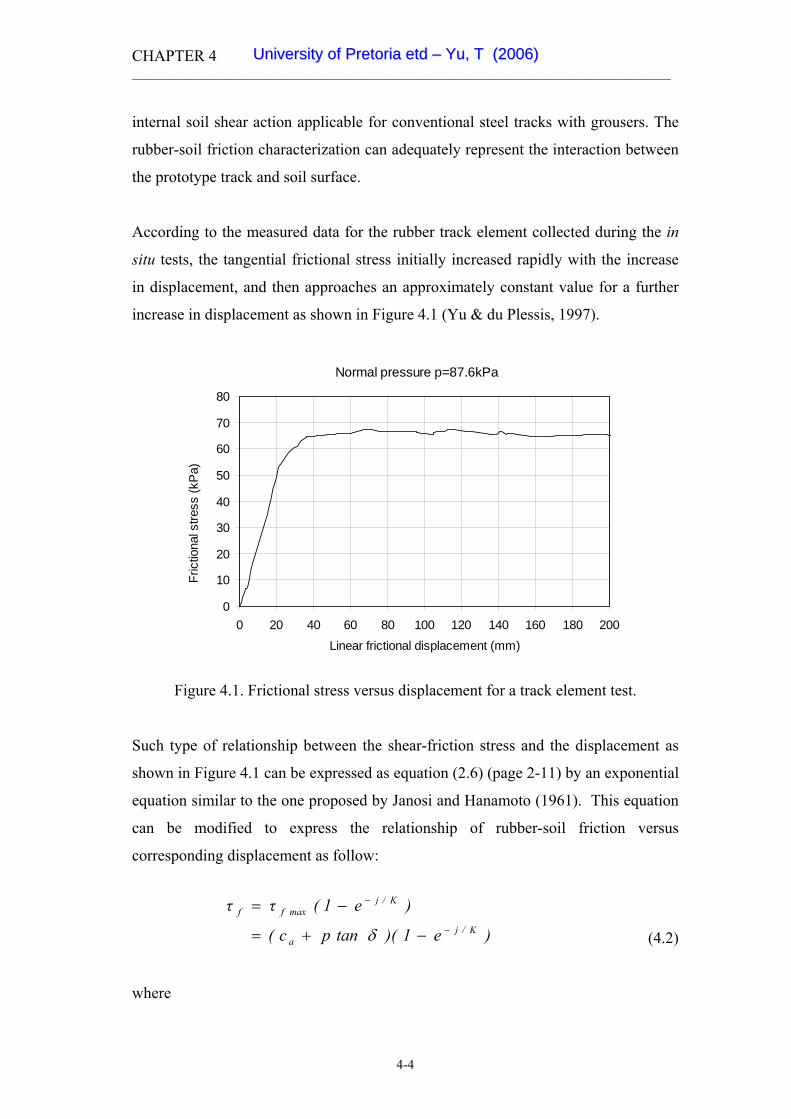
CHAPTER 4 _________________________________________________________________________________

internal soil shear action applicable for conventional steel tracks with grousers. The

rubber-soil friction characterization can adequately represent the interaction between

the prototype track and soil surface.

According to the measured data for the rubber track element collected during the in

situ tests, the tangential frictional stress initially increased rapidly with the increase

in displacement, and then approaches an approximately constant value for a further

increase in displacement as shown in Figure 4.1 (Yu & du Plessis, 1997).

Normal pressure p=87.6kPa

0

10

20

30

40

50

60

70

80

0 20 40 60 80 100 120 140 160 180 200

Linear frictional displacement (mm)

Fric

tiona

l stre

ss (k

Pa)

Figure 4.1. Frictional stress versus displacement for a track element test.

Such type of relationship between the shear-friction stress and the displacement as

shown in Figure 4.1 can be expressed as equation (2.6) (page 2-11) by an exponential

equation similar to the one proposed by Janosi and Hanamoto (1961). This equation

can be modified to express the relationship of rubber-soil friction versus

corresponding displacement as follow:

)e1(ττ K/jmaxff

−−=

)e1)(tanpc( K/ja

−−+= δ (4.2)

where

4-4


CHAPTER 4 _________________________________________________________________________________

τf = rubber-soil frictional stress, (Pa).

j = relative tangential displacement for soil-rubber friction, (m).

K = frictional deformation modulus, (m).

Equation (4.2) reflects the relationship between the horizontal contact frictional

stress and the corresponding slip below the prototype track and soil and is thus used

as the basic soil-rubber frictional characterization.

When compared to the Janosi-Hanamoto equation (2.6), equation (4.2) has the same

format for the equation and also the number of parameters. However, the terms of the

parameters in the equation have different physical meanings. It is the fundamental

relationship for calculating the total tractive effort in the horizontal direction in this

research.

To obtain the parameters related to the frictional characteristics from the field tests,

the method based on the bevameter technique and the procedure reported by Wong

(1989, 1993) and Upadayaya (1994) was adapted.

4.3 CHARACTERIZATION OF THE RELATIONSHIP BETWEEN CONTACT PRESSURE AND SINKAGE

The maximum shear or frictional stress between the tractive device and the terrain

surface directly depends on the applied contact pressure. On a soft terrain surface the

contact pressure is usually related to the sinkage. As reviewed in Chapter 2, several

efforts have been made to identify the exact relationship for contact pressure versus

sinkage in both agricultural engineering and civil engineering applications. To

describe the relationship of the contact pressure and the corresponding sinkage, the

expression proposed by Bekker is still the most common one applied for analytical

modelling methods to predict vehicle performance, especially for the case of soft

terrain surfaces.

4-5


CHAPTER 4 _________________________________________________________________________________

The relationship of contact pressure and sinkage expressed by equation (2.1) can be

used to calculate the contact pressure at each point on the ground contact surface

under the track. In equation (2.1), kc and kφ are parameters related to steel-soil

cohesion and soil-soil friction respectively, while n is the exponent for sinkage

deformation.

For the experimental work, the parameters obtained and the resulted curves from the

field tests are presented in the results.

4.4 ANALYSIS OF THE DISTRIBUTION OF TRACK-SOIL CONTACT PRESSURE

The analysis by Wills (1963) proved that the contact pressure distribution influences

the development of tractive effort. The prediction of the distribution of the contact

pressure is therefore one of the most important issues in analytical traction modelling

for wheels and tracks.

To a large extent, the shape of the track in contact with the terrain surface governs

the distribution of contact pressure. Several typical track deformation shapes can be

considered.

4.4.1 Tractive effort for uniform and trapezoidal pressure distribution

The initial design of the prototype track tested in this project was aimed to achieve an

ideally almost uniform contact pressure distribution by applying the walking beam

concept. For most of the conventional steel tracks, however, the pressure distribution

for a uniformly loaded track was far from being uniform, as reported by many

researchers (Wills, 1963; Wong, 1989). For the practical situations, several factors

influence the pressure distribution at the contact surface including vehicle and track

physical parameters, soil homogeneity and other soil physical properties and in

particular the weight transfer of the tractor. To counterbalance the effect of weight

4-6


CHAPTER 4 _________________________________________________________________________________

transfer, some means of automatic adjustment of the vertical load and consequently

the centre of gravity must be utilized, which is not yet realized for practical field

operations.

When any drawbar pull is applied, the intensity and the distribution of the ground

contact pressure below the track is influenced by weight transfer. To take into

account the effect of the weight transfer, the position of the centre of gravity (CG) of

the test tractor was designed to be located in front of the centre of the track contact

length. When a drawbar pull is applied, the load distribution center of the ground

contact pressure for the track moves rearwards, caused by weight transfer.

In this research project, two simple models of contact pressure distribution are

initially validated and analyzed. One is a uniform distribution whilst the other a

dynamic trapezoidal distribution (Figure 4.2). In the dynamic trapezoidal model, to

predict the distribution of the vertical load, the effect of the weight transfer caused by

drawbar pull is taken into consideration.

For the uniform distribution of the contact pressure, as shown in Figure 4.2 (b), the

value of the ground contact pressure p (Pa) can be calculated from:

(4.3) A/Wp=

where

W = the total vertical load on one track including track weight, (N).

A = the total contact area of one track, (m2).

For the trapezoidal contact pressure distribution, as shown in Figure 4.2 (a) and (c),

the contact pressure changes when the drawbar pull increases. For the static state and

without drawbar pull, the centre of gravity for the vehicle is located in front of the

centre point of the track, thus the contact pressure has a larger magnitude at the front

end and decreases rearwards. As the drawbar pull increases to a specified value, the

transient state of ideal uniform distribution for the contact pressure below the track

4-7


CHAPTER 4 _________________________________________________________________________________

may be reached as shown in Figure 4.2 (b). When the drawbar pull increases further,

the magnitude of the contact pressure at the front end of the track decreases and is

smaller than at the rear (Figure 4.2 (c)).

P

L/2

e

W

V

L/2FrontRear

xL

p2

p1

pp

p1

p2

j=ix

(a)

(b)

(c)

Figure 4.2. The idealized distribution of contact pressure under a track.

In both cases of distribution (a) and (c), if it is assumed that the tractor does not tilt,

one obtains:

4-8


CHAPTER 4 _________________________________________________________________________________

)e1)(tanpc(

)e1(ττK/ix

a

K/jmaxff

−

−

−+=

−=

δ

(4.4) bLW

AWppp ==

+=

221

Where b is the width (m) and L (m) the contact length of one track.

In Figure 4.2 (a), the contact pressure p(x) for any point at a distance x from the track

front contact point can be calculated from:

(4.5) LxL)pp(p)x(p −

−+= 212

where p(x) is the contact pressure at a distance x from the track front contact point.

Similarly, in Figure 4.2 (c), p(x) can be calculated from:

(4.6)

Lx)pp(p)x(p 121 −+=

For either a uniform or trapezoidal contact pressure, it is assumed that the friction-

shear displacement j is linearly proportional to the track slip i. At any point below

the track, with distance x to the front end of the track, the value of the friction-shear

displacement between track and soil, as shown in Figure 4.2, is given by:

(4. 7) ixj =

where i is the slip of the track.

Substituting equation (4.7) into equation (4.2),

(4. 8)

where the contact pressure p is also a function of x and is expressed by one of

equations (4.3) to (4.6).

4-9


CHAPTER 4 _________________________________________________________________________________

When the frictional stress τf is integrated along the contact length, the total tractive

effort Ft can be predicted as:

(4.9) dx)e1](tan)x(pc[2

dx)x(2FL

0

K/ixa

L

0 ft

∫∫

−−+=

=

δ

τ

4.4.2 Tractive effort for a rigid track model with tilt angle

On a deformable terrain surface, however, the track-soil contact surface is usually

inclined towards the rear of the track, depending on the drawbar height and drawbar

pull. With further assumption of a tilt angle β, the parameters to describe the track-

soil interaction are illustrated in Figure 4.3.

As shown in Figure 4.3, for equilibrium in the vertical direction:

dx]sin)x(cos)x(p[bWL

0 f∫ += βτβ (4.10)

For equilibrium in the horizontal direction:

∫ −=L

0 ft dx]sin)x(pcos)x([bF ββτ (4.11)

and the rolling resistance Rr:

(4.12) =R ∫L

0r dxsin)x(pb β

4-10


CHAPTER 4 _________________________________________________________________________________

WV

ω

β xL

zf

zp(x)

τf(x)

Fh

Figure 4.3. Side view of the track-soil interaction with the inclusion of a tilt angle.

In the above equations (4.10-4.12), the contact pressure of the track at any point in

contact with the terrain depends on the corresponding sinkage at the specific point,

whilst the sinkage can be calculated from the initial sinkage of the front wheel zf0 and

the tilt angle β.

By substituting the values of τf(x) and p(x) into the above equations, the tractive

effort Ft and the rolling resistance Rr can be predicted.

The calculation for traction can be initiated by assuming that the front and rear

wheels support the total static vertical load proportionally. The static sinkage of the

front and the rear wheels can be calculated by applying the equation proposed by

Bekker (1960). The tilt angle can also be calculated according to the load distributed

on the front and rear wheels respectively.

To avoid a negative tilt angle, the tilt angle is initially assumed to be zero, due to the

fact that the CG of the tractor is located in front of the middle point of the track in a

longitudinal direction. The tilt angle remains zero until the vertical load is distributed

equally between the front and the rear wheels. With further increase in drawbar pull,

the load on the rear wheels increases and the load on the front wheels decreases by

the same numeric value which was derived from the weight transfer. The tilt angle is

4-11


CHAPTER 4 _________________________________________________________________________________

taken into consideration as soon as the load on the rear wheels is larger than the load

on the front wheels.

Therefore, one of the advantages of this model is that the effect of load transfer can

be accounted for when the drawbar pull changes, in addition to the uniform or

trapezoidal contact pressure distributions.

4.4.3 Tractive effort for the flexible track model

If the designed walking beam effect of the prototype track materializes, the track

operates similar to a wheel of very large diameter which may result in a very uniform

distribution of contact pressure. The track-soil interaction can be solved by applying

one of the idealized models as shown in Figures 4.2 and 4.3.

However, when the centre wheels were not forced onto the track, it was difficult to

achieve the idealized uniformly distributed contact pressure as envisaged by the

original design concept. Most likely, the track was flexible and be deformed at the

section between the front and the rear wheels, being influenced by several factors,

particularly the terrain characteristics and the track tension. When the track tension

was not automatically adjusted or not sufficient to form the large circle in

equilibrium with the terrain, the section of the track between the front and rear

wheels would be deflected upwards and form a curved interacting shape with the

terrain surface. The shape of this interaction surface would, to a large extent, govern

the distribution of the contact pressure.

While the ideal contact pressure distribution is as shown in Figure 4.2, based on the

practical observations and preparatory tests on a soft terrain surface (Yu and du

Plessis, 1997) definitive peak pressures were observed below the front and rear

wheels. The shape of the flexible interaction surface between the track and the soil

was assumed to be as shown in Figure 4.4.

4-12


CHAPTER 4 _________________________________________________________________________________

For the shape shown in Figure 4.4, the contact surface of the track and deformable

terrain can be divided into two typical segments, one in contact with both the wheel

and terrain, such as segments of ABC and FGH, and another in contact only with the

terrain, such as segment CDEF.

WV

ω

β

L

zf

zX Z

α1fα1r

α2f

r

R

Figure 4.4. The flexible deformation model for track-soil interaction.

It was assumed that the front wheels initially had a sinkage of zf, and the shape of the

curve between the front and the rear wheels, i.e. the segment CDEF in contact only

with the terrain surface, was circular in shape, with radius R.

On a soft terrain surface, the inflation pressure of the driving and tension wheels was

relatively high to optimize the friction drive. It is, therefore, reasonable to assume

that the wheels have characteristics similar to that of rigid wheels. The shape of the

contact segments ABC and FGH therefore are circular, with the same diameter as the

tyres.

zr

α2r

A

B

CDE

F

GH

α

α1rα2f

α

4-13


CHAPTER 4 _________________________________________________________________________________

On the basis of the assumptions above, the following relevant geometrical

parameters were derived from the track-soil configuration as illustrated in Figure 4.4.

)1(cos 11 r

z ff −= −α (4.13)

]2/)sin[(2 21

22

fr

ZXRαα +

+= (4.14)

where

(4.15) )sin(sinrcosLX fr 21 ααβ +−=

and )cos(cosrsinLZ fr 21 ααβ −−= (4.16)

)L/)zz((sin fr

1 −= −β (4.17)

(4.18) βαα 221 += fr

If a rigid wheel on a soft terrain was accepted, the sinkage of the front and the rear

wheels could be determined by applying the analysis as proposed by Bekker (1956,

1960):

The sinkage

)1n2/(2

c

ff r2)kb/k)(n3(b

W3z

+

⎥⎥⎦

⎤

⎢⎢⎣

⎡

+−=

φ(4.19)

and sinkage

)1n2/(2

c

rr r2)kb/k)(n3(b

W3z+

⎥⎥⎦

⎤

⎢⎢⎣

⎡

+−=

φ (4.20)

4-14


CHAPTER 4 _________________________________________________________________________________

where Wf and Wr represented the vertical load on the front and the rear wheels

respectively whilst b was the track width

In the above analysis, the radius of the deformed track segment in contact with the

terrain surface directly depended on the exit angle of the front wheels, the distance

between the front and the rear wheels and the wheel diameter.

Wong (1989) indicated that the entrance and the exit angles for a pneumatic tyre

were interrelated and the relationship was governed by the terrain response to

repetitive contact loading, but the relationship was not specified or suggested. Due to

the fact that the rebound of the terrain was limited by the track tension and the track

was not definitely flexible, the exit angle was expected to be smaller than the value

calculated for the case of a pneumatic tyre.

Okello et al (1998) proposed the use of a constant C to relate the entrance and the

exit angles as:

fr C 12 αα = (4.21)

However, no method to determine the value of C was mentioned.

From the curves of the repetitive contact loading, it could be seen that when the

terrain stiffness was larger, the contact pressure decreased more rapidly during the

unloading cycle and the elastic rebound of the terrain took a shorter period of time. It

was considered that the slope angle of the unloading curve could be used to derive

the exit angle. No practical conclusions on the entrance and exit angles were drawn

from the unloading-reloading curves and it needs more experimentation to proof such

a relationship.

Karafiath and Nowatzki (1978, pp 386-387) proposed that the exit angle be taken as

10 degrees for entry angle variations from 30 to 60 degrees. For entry angles of less

than 30 degrees, it should be reduced by half the difference between the entry angle

4-15


CHAPTER 4 _________________________________________________________________________________

and 30 degrees. Based on this method, the exit angle was therefore calculated as 0

when the entry angle was less than 10 degrees. By considering the effect of the track

tension on soft terrain for the proposed model, the exit angle was determined as one

third of the entry angle.

The track contact surface was divided into n segments of different configuration, and

the equilibrium equations for the track were expressed as:

In the vertical direction,

(4.22) ∑ ∫

=

+ +=n

fiii

1i0 fii

1i d)cossinp(rb α

ααατα

∑ ∫

∑

=

=

+=

=

1i

n l

n

1ii

i

i dx)cossinp(b

WW

ατα

In the horizontal direction,

∑ ∫

∑ ∫

∑

=

=

=

+ +=

+=

=

n

1ifiii

n

1i

l

0 fii

n

1iitt

1i

i

i

d)sincosp(rb

dx)sincosp(b

FF

α

ααατα

ατα

(4.23)

In the above equations, the subscription i indicates the ith segment which has the

length of ℓi with radius of ri, entrance angle of αi and exit angle of αi+1 under

consideration, as illustrated in Figure 4.4. It can be seen that all the variables in the

above equations can be expressed as functions of the angle α of the wheels.

To describe the relationship of the frictional-shear stress versus the slippage (j), an

analysis based on Wong’s model for a steel track with ground wheels (Wong, 1993),

was adopted.

4-16


CHAPTER 4 _________________________________________________________________________________

The slip velocity of any point on the surface of the track-soil interaction, relative to

the terrain surface, was the tangential component of the absolute velocity:

]i)sinα(1-1[rω i)sinα-1(rrω

VsinαVV tj

−=−=

−=

ω

(4.24)

The friction-shear displacement (j) along the track-terrain interface was obtained by

integrating the slip velocity from the point where friction-shear started to the

specified point under consideration:

(4.25) x)i(

d]i)sin(1-1[r

dt]i)sin(1-[1rj

i

1f/

t

0

−−=

−=

−=

∫∫

−

12

l

αα

αωα

απ

where ℓ is the contact length between the specified point to the point where soil

contact started, and x was the corresponding horizontal distance between the specific

point and the initial soil contact point. The rotational angle α for each segment was

considered. The value of αi was calculated according to the corresponding

configuration of the segment. Therefore the integrated value of j was also calculated

for any point within each segment. For instance, for the segment ABC, the friction

and shear displacement j at any point was calculated as:

)]sin)(cosi1())2/([(r

))]2/cos()(cosi1())2/([(rj

f1f1

f1f1

αααπα

απααπα

−−+−−=

−−−+−−=

(4.26)

Whilst for a point within the segment of the track in contact only with the terrain

surface CDEF, j was calculated from:

)]sin)(cosi1())2/([(r )]sin)(sini1()[(r

dsin)i1(1[rd]i)sin(1-1[rj

f2f2

f2f1f2f1

2/

2/

2/ f2

f2

1f

αααπα

αααα

ααααα

απ

απ

απ

−−+−−+

+−−+=

−−+−= ∫∫ −

+

−

(4.27)

4-17


CHAPTER 4 _________________________________________________________________________________

4-18

Similarly, for a point within the segment FGH, the displacement was determined

from:

)]sin)(cosi1())2/([(r )]sin)(sini1()[(R

)]sin)(sini1()[(r

d]i)sin(1-1[r

dsin)i1(1[Rd]i)sin(1-1[rj

r1r1

r1f2r1f2

f2f1f2f1

2/

2/

2/

2/

2/

1r

r1

f2

f2

1f

αααπα

αααα

αααα

αα

αααα

α

απ

απ

απ

απ

απ

−−+−−+

+−−++

+−−+=

−+

−−+−=

∫

∫∫

−

+

−

+

−

(4.28)

4.5 THE PREDICTION OF MOTION RESISTANCE

The motion resistance of the prototype track Rr can be expressed as:

Rr= Re +Ri (4.29)

Where Re is the external resistance and Ri is the internal track resistance.

For the models as discussed in the Section 4.4.1 (page 4-5), the external motion

resistance between the track and the terrain surface is mainly due to the soil

compaction below the track. To simplify the procedure for predicting the

performance, only the rolling resistance for soil compacting was taken into

consideration.

If the contact pressure on the track-terrain interface is distributed uniformly, which is

the case for an ideal ground pressure distribution based on the initial design, the

motion resistance for compacting soil was expressed by Bekker (1960):

nn

nc

e bLW

kbknbR

/)1(

)/1()/)(1(

+

⎟⎠⎞

⎜⎝⎛

++=

φ(4.30)


CHAPTER 4 _________________________________________________________________________________

Observations based on the preliminary test results (Yu and du Plessis, 1997) proved

(4.31)

Equation ith track segment, whilst ri is

he internal loss is mainly caused by friction and relative movement and associated

nder operational conditions, rubber materials have elastic characteristics. During

∑ ∫

∑ ∫

∑

=

=

=

+=

=

=

n

ii

n

i

iie

i

i

i

dxpbr

dxpb

RR

1

10

1

1 sin)(

sin)(

α

ααα

αl

l

that the contact pressure distribution was not as uniform as expected. Other possible

pressure distributions, such as the rigid and the flexible track models described in the

preceding sections, should therefore also be considered. For both rigid and flexible

models, the rolling resistance was attributed to the total horizontal component of the

contact pressure in the direction opposite to travelling. The contact pressure was

expressed as a function of the rotational angle of the track segment α for the flexible

track model as shown in Figure 4.4. The motion resistance can be predicted by

summation of the motion resistance generated by each segment of the track as shown

in the following equation:

n

In (4.31), ℓ is the corresponding length of the i

either the radius of the wheels or the virtual radius of the circular curve of the track

in contact only with the terrain surface.

T

friction between the track elements. The track tension of the prototype traction

system was designed to be adjustable. If the track tension was adjusted to be higher

than the maximum tractive effort between the track and terrain surface, the slip

resulting would be kept to a minimum.

U

this action extra internal losses were therefore caused by cyclic reshaping of the

rubber tracks and the wheels with hysteresis and heat build up. An analysis of the

internal resistance will be addressed in the next section.

4-19


CHAPTER 4 _________________________________________________________________________________

The total motion resistance can be calculated based on equation (4.29) after the

external and internal resistances are obtained.

4.6 INTERNAL TRACK RESISTANCE AND THE FRICTION DRIVE BETWEEN THE WHEEL AND THE TRACK

The prototype track is tensioned to a specified level by a hydraulic cylinder and

locked by a threaded rod and lock nuts.

The track tension is a critical factor for the frictional torque transfer between the

drive wheels and the internal track surface.

If the rubber surfaced track stretched by the drive wheels is considered as a rubber

belt and a rubber pulley, the analytical results for belt conveyers and friction drives

may be utilized to explain the relationship of tension and frictional drive force. When

the rubber belt track travels on a smooth rigid surface and the traction force is

assumed to increase linearly along the ground contact length of the track, as shown in

Figure 4.5, the following relationship can be established according to basic theory of

belt friction (Green, 1955):

)1(0

00

0tt

eT

TeT

TTF

−′

′

=

−=

−=

ϕ

ϕ

μπ

μπ

(4.32)

where

T0 = track pre-tension, (N).

Tt = maximum track tention, (N).

Ft = tractive effort, (N).

μφ = friction coefficient between contact surfaces.

π´ = wrap angle = 180°.

4-20


CHAPTER 4 _________________________________________________________________________________

T0

T0

T0

Tt

V

Tr Tf

Ft

ω

Figure 4.5. Simplified distribution of the track internal tension during forward

movement.

When the values of the track pre-tension T0, the wrap angle and the friction

coefficient are set, the tractive effort Ft is the limitation within which slippage is

minimized. Therefore the higher the track tension, the larger the traction that can be

transfered. On the other hand, the magnitude of the track tension is limited by the

dimensions of the sub-frame structure, the strength of the track and other design

factors.

As observed in practice, small amounts of slippage occur as soon as the friction drive

is loaded, although it is not easily measurable when the drawbar pull is small. The

loss caused by this slippage may be accepted as 3-5% of the total power transmitted

by the traction device which represents a typical situation for a rubber belt conveyer

(Green, 1955).

In this research, to simplify the calculation for modelling, a decrease of 3% of the

total tractive effort was accepted to account for internal bending and slip losses,

regardless of the speed.

4-21


CHAPTER 4 _________________________________________________________________________________

4-22

4.7 TOTAL DRAWBAR PULL OF THE PROTOTYPE TRACK

The total drawbar pull Fh is the difference between the tractive effort and the motion

resistance and can be expressed as:

(4.33) rth RFF −=

where Ft is the resultant total force in the direction of movement which can be

obtained by integration or derived from the analysis of tangential stresses and contact

pressure. Rr is the total motion resistance.

Since the contact pressure and the tangential stress are functions of the track sinkage

and the track slip respectively, the track motion resistance Rr and the tractive effort Ft

also vary with the track slip. Based on equation (4.33), the relationship of drawbar

pull and the track slip can be predicted.

4.8 THE COEFFICIENT OF TRACTION AND TRACTIVE EFFICIENCY

The coefficient of traction Cct is the ratio of tractive effort to the vertical load of the

track and expressed by:

WFC t

ct =

ωη

T2VF

PP h

in

out ==

(4.34)

The tractive efficiency η is the ratio of the output to input power of the track and

expressed as:

(4.35)

where

η = tractive efficiency.


CHAPTER 4 _________________________________________________________________________________

Pin = input power, (kW).

Pout = output power, (kW).

Fh = total drawbar pull, (N)

V = travel velocity, (m/s)

T = input torque for one side shaft, (Nm).

4.9 MODELLING PROCEDURE

For both the flexible track and the rigid track models, the static vehicle weight was

accepted to be supported only by the wheels. The sinkage of the front wheels were

calculated based on Bekker’s (1956, 1960) sinkage equation for solid wheels

(equations 4.19 and 4.20). The sinkage of the rear wheels were accepted to be equal

to that of the front wheels until the load increase caused by weight transfer, which

lead to additional rear wheel sinkage.

The contact pressure at any point on the interacting surface was calculated based on

the pressure sinkage relationship proposed by Bekker with equation (2.1) after which

the sinkage at each point on the contact surface was determined by initial

assumptions and the configuration of the track-terrain contact profile as described in

the previous sections of this chapter. The tilt angle β was also taken into account for

the contact pressure caused by sinkage.

The accumulated displacement j was calculated by equation (4.7) or equations (4.26)

to (4.28). Equation (4.7) (p 4-9) was validated for the idealized contact pressure

distribution. Equations (4.26) (p 4-17), (4.27) (p 4-17) and (4.28) (p 4-18) were

applicable for the segments ABC, CDEF and FGH (Figure 4.4, p 4-13) respectively

for the flexible track model. The tangential stress was then calculated from equation

(4.2) (p 4-4), as described in the previous sections of this chapter. The total thrust for

a specific level of slip was calculated by applying equation (4.11) (p 4-10) for the

idealized uniform distribution or (4.23) (p 4-16) for the flexible track model. The

parameters related to rubber-soil friction characterization were obtained from

bevameter tests.

4-23


CHAPTER 4 _________________________________________________________________________________

When the motion resistance was calculated by any of the equations (4.12) (p 4-10)

for the uniform pressure distribution model, or equations (4.30) (p 4-18) and (4.31)

(p 4-19) for the flexible track model respectively, the drawbar pull was the difference

between the total tractive thrust and the calculated motion resistance.

The tractive thrust as well as the motion resistance could be calculated by either

computer programming or spreadsheet coding. To utilize its advantage of simplicity,

the spreadsheet method was mainly used for the calculations for this research.

The final results from the calculations were expressed as the relationship of either the

tractive force or the drawbar pull versus the slip as was predicted.

4-24


CHAPTER 5 _________________________________________________________________________________

CHAPTER V

INSTRUMENTATION, CALIBRATION AND EXPERIMENTAL PROCEDURE

5.1 INTRODUCTION

To prove the proposed theoretical model for the traction performance of the tracked

vehicle on soft terrain surface based on the analytical method, in situ soil

characterization was necessary. In this research project, the bevameter technique was

used to acquire soil characteristics for shear strength, rubber-soil friction as well as

the pressure-sinkage relationship.

For validation of the predicted results, a series of full-scale drawbar pull tests were

conducted in the field. The parameters measured during the drawbar pull test

included the drawbar pull, the torque to one side drive shaft of the tractor and the

theoretical and actual travel speeds was based on which the total slippage was

calculated. The slip between wheel and track measured manually by means of marks

on the wheel and the track to derive the difference between the calculated wheel

travel distances to the measured track travel distance after a certain number of

revolutions of the wheel.

The contact and the tangential forces on the ground contact surface between a track

element and the soil were also measured by using two small specially designed

extended octagonal ring transducers, mounted on the track basis. From the measured

contact force, the distribution of the contact pressure along the track was derived.

The total tangential tractive effort was calculated based on the summation of the

measured tangential forces.

5-1


CHAPTER 5 _________________________________________________________________________________

All the experimental work was conducted under field conditions at the Experimental

Farm, University of Pretoria. To identify the influence of the soil water content on

drawbar performance it was decided to perform the tests under three different values

of soil water content, controlled by irrigating the test site several days before a test.

In order to achieve realistic test conditions as expected, the field was carefully

chosen and disk ploughed. The tests were also conducted during the dry winter

season to eliminate the influence of rainfall.

A computerized data acquisition and logging system was built and used to pre-

process and record all the data concerned.

5.2 APPARATUS FOR SOIL CHARACTERIZATION

To obtain the soil parameters necessary for the traction modelling based on the

analytical methods, an instrumented apparatus applying the bevameter technique was

built in the Department of Agricultural Engineering, University of Pretoria (Yu,

1996). This linear shear and soil sinkage apparatus was similar to the one originally

developed at the University of California, Davis Campus (Upadhyaya et al, 1993).

The instrumented apparatus as shown in Figure 5.1, can be used to measure:

• linear soil shear and frictional characteristics for steel-soil and rubber-soil

contact respectively;

• soil contact pressure-sinkage parameters; and

• soil cone index.

The main frame (M) was carried by a front mounted tractor three point linkage (L).

A double acting hydraulic cylinder and set of loading blade springs (B) applied a

predetermined constant vertical load to the main frame (M) and adjustable feet (A).

5-2


CHAPTER 5 _________________________________________________________________________________

The grouser carrier frame (F) was moved horizontally by a hydraulic cylinder (H2)

supported by two horizontal brass bearings sliding over round stainless steel rod

slides (S2). To accommodate slip sinkage during the test the anchor of the traction

cylinder (H2) slides vertically on a brass bush and rod (S3). To ensure minimal

frictional influence on the horizontal shear force, measured by the load cell between

the grouser carrier frame and piston assembly (H2), the grouser was carried by four

identical vertical adjustable arms (L1) with ball joints.

L

BS3

MV

C C

S2

HL

A

B2

S1

2

1

2

1

F

1

2

`H1

A – adjustable feet B – loading blade springs B2 – moving blocks

C1 – control lever C2 – second control lever F – carrier frame

H1 – vertical cylinder H2 – piston assembly L – three point linkage

M – main frame S1 – vertical piston rod S2 – rod slides

S3 – brass bush and rod V – pressure control valve

Figure 5.1. Linear shear meter used for soil shear, soil-rubber friction as well as

sinkage characterization.

5-3


CHAPTER 5 _________________________________________________________________________________

Two separate hydraulic circuits were used to prevent interaction between the vertical

and horizontal loading. The vertical force was applied by a pump and circuit, with a

hydraulic cylinder between the main frame (M) and unit with two parallel moving

blocks (B2). The vertical load cell was mounted between (B2) and the grouser carrier.

The applied vertical force was kept constant during slip sinkage by supplying surplus

oil and using a special adjustable pressure control valve (V). During the test the

vertical load was applied with the supply control lever (C1) fully open and the control

valve (V) set at a specific release pressure, with the surplus oil flowing back to the

tank.

The second control lever (C2) activated the second hydraulic circuit and supplied oil

to the horizontal cylinder (H2) whilst the vertical hydraulic cylinder (H1) followed

the slip sinkage action and applied a constant vertical load. The vertical and

horizontal displacement of the grouser was recorded via two rotational

potentiometers with woven string and a rotary spring for automatic return.

Two industrial S-type weighing scale load cells were used to measure the applied

vertical and horizontal loads independently. The shear grousers, sinkage plates and

cone penetrometer with different shapes, dimensions, and surface materials could

easily be removed and replaced when necessary.

The analog signals from the load cells and the potentiometers had to be pre-

processed by an A/D converter before being recorded by the data acquisition system.

Three sinkage steel plates with different dimensions were used to characterize the

soil pressure-sinkage relationships. Two different steel shear grousers were used to

obtain the soil shear characteristics, whilst a standard rubber-covered track element

was used to measure the rubber-soil frictional characteristics.

Figure 5.2 shows the grouser shear plates, the sinkage plates, the track element and

the cone penetrometer used for soil characterization with the instrumented bevameter.

5-4


CHAPTER 5 _________________________________________________________________________________

The dimensions of the shear grousers and the sinkage plates are shown in Table 5.1

and Table 5.2 respectively.

(a) shear grousers (b) sinkage plates

(c) track element (d) cone penetrometer

Figure 5.2. Components used for soil characterization.

Table 5.1. Dimensions of the rectangular steel shear grousers and the rubber

track element.

Dimension Length, mm Width, mm Grouser height, mm

Steel shear grouser 240 60 10

Steel shear grouser 220 80 12

Rubber track element 500 70 Smooth rubber surface

5-5


CHAPTER 5 _________________________________________________________________________________

Table 5.2. Dimensions of the steel sinkage plates.

Sinkage plate Width, mm Length, mm Aspect ratio (L/W)

No. 1 70 210 3

No. 2 60 240 4

No. 3 55 285 5.18

5.3 THE EXTENDED OCTAGONAL RING TRANSDUCERS FOR MEASURING THE DISTRIBUTION OF CONTACT PRESSURE AND TANGENTIAL STRESS

5.3.1 Design of the transducer

Two identical extended octagonal ring transducers were built in order to measure the

distribution of contact pressure and tangential stresses.

The basic shape and dimensions of the octagonal ring transducer are shown in Figure

5.3.

The values of Lo and ro were chosen to accommodate the limited space available

between the track element and the base plate over the track cable assembly. The

value of b was chosen to provide for sufficient supporting area and stiffness to mount

the transducer onto the track. The transducers were machined from a solid block of

EN24 alloy steel, and heat-treated for an ultimate tensile strength of about

1500MN/m2 on which the preliminary design was based. Both high sensitivity and

sufficient stiffness within the elastic deformation range was necessary. By applying

the equations as reviewed in Chapter 2, the thickness to, at the middle point of the flat

surface was initially calculated as 1.9mm. The vertical force was accepted as 2000N

with an allowable working stress of 750MN/m2. For machining purpose, the value of

5-6


CHAPTER 5 _________________________________________________________________________________

to was eventually adjusted to 2mm. The dimensions for the two transducers are

shown in Table 5.3.

Figure 5.3. Design parameters and forces for the extended octagonal ring

transducer.

Table 5.3. The dimensions of the octagonal ring transducers.

ro, mm Lo, mm to, mm bo, mm φFx, deg φFy, deg

16 55 2 20 90 45

The nodal angle for force Fx was determined as 90° by trial and error fixing of the

strain gauges at different angles with the least interference on force Fx by force Fy

and vice versa,. For force Fy, the nodal angle was identified as 45°.

The ratio of ro/to=8 is larger than 5 and is sufficiently large for thin ring theory to be

accepted as valid on which the design was based (Godwin, 1975).

5-7


CHAPTER 5 _________________________________________________________________________________

5.3.2 Calibration and installation of the transducers

For each extended octagonal ring transducer, eight 120Ω strain gauges were used to

form two Wheatstone bridges. After the strain gauges were fixed and the circuits

connected, the two transducers were calibrated using a special frame on which the

horizontal and the vertical loads were applied independently. The excitation voltage

to the bridges was 5 volt and the outputs for calibration were measured with a

Hewlett-Packard high-sensitivity multi-meter.

The preliminary calibrations showed some unacceptably high cross sensitivity errors

for the bridge measuring force Fy caused by force Fx (Yu & du Plessis, 1996).

Further investigation and modifications were undertaken to correct the error by

inserting two thicker steel spacers (B in Figure 5.4) on both mounting surfaces of the

transducer to ensure that the elastic deformation of the transducer was not interfered

with by improper constraints as shown in Figure 5.4.

Prior to the field tests, the two transducers were finally calibrated to obtain the results

as shown in Figures 5.5 to 5.8. The regression data proved that the outputs for both

transducers were highly linear with the correlation coefficients ≥ 0.998 over the full

load range tested. The recorded cross sensitivity error for the two transducers was

less than 2%. The line is shown at the bottom of each graph. The calibration results

are shown in Table 5.4.

5-8


CHAPTER 5 _________________________________________________________________________________

Rubber tread

Steelprops×4

Steel cables

2 extended octagonalring transducers

1 2

7

5 6

34

8

(C) (D) (E)

(A)(B)

(B)

FyFx1 2

34

+ -

- +Fy

ΔvOutput

v Input

5 6

87

- +

+ -Fx

ΔvOutput

v Input

Centraldividerflanges

70mm

200m

m

Inner rubberfriction surface

Figure 5.4. The installation of the octagonal ring transducers on

the track element.

Vertical calibration, transducer 1

R2 = 0.9998

0

5

10

15

20

25

0 500 1000 1500

Vertical load (N)

Out

put (

mV

)

Vertical outputHorizontal output

Figure 5.5. Vertical calibration of the octagonal ring transducer 1.

5-9


CHAPTER 5 _________________________________________________________________________________

Horizontal calibration, transducer 1

R2 =0.9999

0

5

10

15

20

25

0 200 400 600 800 1000 1200

Horizontal load (N)

Out

put (

mV

)

Horizontal outputVertical output

Figure 5.6. Horizontal calibration of the octagonal ring transducer 1.

Vertical calibration, transducer 2

R2 = 0.9999

0

5

10

15

20

25

0 200 400 600 800 1000 1200 1400 1600

Vertical load (N)

Out

put (

mV

)

Vertical outputHorizontal output

Figure 5.7. Vertical calibration of the octagonal ring transducer 2.

5-10


CHAPTER 5 _________________________________________________________________________________

Horizontal calibration, transducer 2

R2 = 0.9999

0

5

10

15

20

25

0 200 400 600 800 1000 1200

Horizontal load (N)

Out

put (

mV

)

Horizontal outputVertical output

Figure 5.8. Horizontal calibration of the octagonal ring transducer 2.

Table 5.4. Calibration results for the two octagonal ring transducers.

Transducer 1 Transducer 2

Vertical load FV

Horizontal load

FH

Vertical load FVHorizontal load

FH

Sensitivity

(mV/N⋅V) 0.62180 0.52453 0.65049 0.52534

Correlation

coefficient 0.99981 0.99991 0.99995 0.99992

5-11


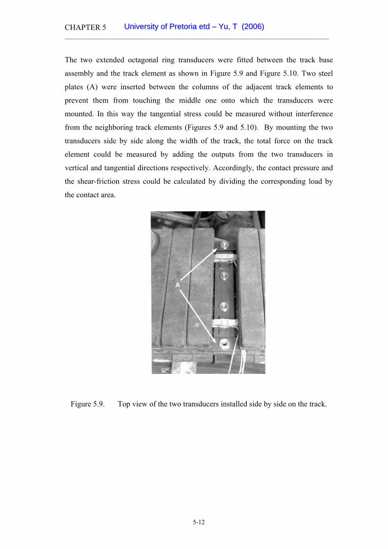
CHAPTER 5 _________________________________________________________________________________

The two extended octagonal ring transducers were fitted between the track base

assembly and the track element as shown in Figure 5.9 and Figure 5.10. Two steel

plates (A) were inserted between the columns of the adjacent track elements to

prevent them from touching the middle one onto which the transducers were

mounted. In this way the tangential stress could be measured without interference

from the neighboring track elements (Figures 5.9 and 5.10). By mounting the two

transducers side by side along the width of the track, the total force on the track

element could be measured by adding the outputs from the two transducers in

vertical and tangential directions respectively. Accordingly, the contact pressure and

the shear-friction stress could be calculated by dividing the corresponding load by

the contact area.

Figure 5.9. Top view of the two transducers installed side by side on the track.

5-12


CHAPTER 5 _________________________________________________________________________________

Figure 5.10. Side view of the two octagonal ring transducers installed between the

track element and the track base assembly.

5.4 INSTRUMENTATION FOR MEASURING TORQUE, SLIP AND DRAWBAR PULL

5.4.1 Instrumentation for measuring the side shaft torque

By using a special differential system in the tractor drive train, the torque is equally

divided between the two side shafts under normal operational conditions. The drive

torque and speed are also equally split to the two side shafts for straight line traveling.

To simplify the instrumentation for measurement, it was decided to measure the

torque and the speed for only one side shaft as torque was equally split between the

two side shafts by the interlinked differential.

Wire-type strain gauges were chosen to measure the side shaft torque and the circuit

was connected into Wheatstone bridges (Figure 5.11). To reduce the noise errors

during the signal transfer, the output signal for the torque was firstly amplified and

conditioned by a circuit fixed to the rotating shaft. The amplified signal was

transmitted via a slip ring and a cable system to the data acquisition system. The

torque transducer was calibrated prior to the re-assembly of the drive axle by using a

5-13


CHAPTER 5 _________________________________________________________________________________

three meter long steel arm fixed to the drive shaft and step by step loading it by

standard weights. The calibration data for the torque transducer is shown in Figure

5.12.

45°

45°

2

14

3

Vo Vi

R1

R2

R4

R3

+

+

-

-

Figure 5.11. The strain gauges and the circuit to measure the side shaft torque.

R2 = 0.9994

0123456789

10

0 5000 10000 15000 20000 25000 30000Torque (N-m)

Out

put (

mV

)

Figure 5.12. The calibration results for the torque transducer.

5-14


CHAPTER 5 _________________________________________________________________________________

5.4.2 Instrumentation for measuring speed and slip

Two speed sensors using photoelectric counters were built to measure the speeds

(Figure 5.13). The sensor consisted of a circular and thin transparent plastic disk with

uniformly distributed radial black printed stripes at the outer edge (Figure 5.13, A)

housed in a circular aluminum housing (B) and a micro optical emitting switch (C)

on the side of the box. The optical switch sensed the number of the radial black

stripes passing the slot which were subsequently recorded as a frequency signal by a

special pulse counter circuit.

Figure 5.13. Construction of the speed transducers.

Figure 5.14 shows the two instrumented speed transducers mounted on the side shaft

of the tractor.

The frequency signals from the speed transducers and the analog signals from the

torque transducer on the side shaft were transferred via a slip ring unit (A) with

special carbon brushes (Figure 5.14). The rotational speed of the rear side shaft was

recorded by the speed transducer unit (B). The true ground speed was recorded by

5-15


CHAPTER 5 _________________________________________________________________________________

5-16

the speed transducer unit (D) fixed to a drum driven by a cable and anchored to the

soil surface. The cable was rewound by winch (C) and braked by (E) to prevent the

cable from overrunning. Wheel (F) was used for changing the cable direction.

A - slip ring B – speed transducer unit for theoretical speed

C – winch D – speed transducer unit for actual speed

E – winch brake

Figure 5.14. The speed transducers, the brush and rotational slip ring unit mounted

on the side shaft of the tractor.

The total slip of the track St, including wheel to track slip, was obtained by

measuring the theoretical speed Vt and the ground speed V of the tractor.

%100V

VVSt

tt ×

−= (5.1)

The angular speed ω of the shaft of the aluminum unit was obtained based on the

frequency of the speed pickup by applying equation (5.2):

(5.2) n/fπω 2=


CHAPTER 5 _________________________________________________________________________________

Where n is the total number of the black stripes for 360 degree engraved circle on the

plastic sheet.

One of the two aluminum counter units was directly mounted on the extended part of

the side drive shaft (Figure 5.13 (A)) and was used to measure the theoretical speed

Vt as:

tt

tt2

ttt

fC fr4

r2V

==

=

π

ωπ

(5.3)

Where

rt = the rolling radius of the track, (m).

ωt = the theoretical angular speed, (rad/s).

ft = the frequency recorded up by the theoretical speed sensor.

Ct = a constant.

The travel distance for a specified number of revolutions of the drive wheel Nt was

measured when the crawler tractor was propelled by its own engine but with zero

drawbar pull on concrete road surface. Then the travel distance for the same

specified number of revolutions of the drive wheel Nt was measured again when the

crawler tractor in neutral gear was towed by another tractor. The rolling radius of the

track was calculated based on applying the average travel distance Lt from the above

two runs.

Thus,

t

tt N2

Lrπ

= (5.4)

The effective radius of the drum was determined by taking the effect of cable

diameter into account. When the drum was driven by cable winding over it, the

revolutions of the drum Nd were counted and the corresponding travel distance of the

cable Ld measured. The effective radius of the drum was therefore calculated by:

5-17


CHAPTER 5 _________________________________________________________________________________

5-18

d

dd N2

Lrπ

=

d

fC fr4

r2V

==

=

π

(5.5)

Similarly, the ground travel speed V can then be obtained as:

dπ ω

aa

ad2

(5.6)

Where

rd = effective radius of the drum, (m).

ωd = angular speed of the pulley, (rad/s).

fa = the frequency recorded by the actual speed sensor.

Ca = a constant to calculate the theoretical speed related to rd and π.

For the above instrumented device, the recorded slip was the total slip including the

wheel-track slip and the track-soil slip.

The wheel-track slip was measured for the field tests by manually marking the tyre

surface and the track element. The first marks were made on the tyre and the

specified track element at the same time. After several revolutions, the travel

distances of the marked point on the tyre and the marked track element were

measured and compared to obtain the difference between the two. Then the slip

between the wheel and the track was determined.

5.4.3 Instrumentation for measuring drawbar pull

The drawbar pull was measured by mounting a 10 ton industrial load cell, from a

local supplier, namely Load Cell Services, between the tested crawler tractor and one

or two loading wheeled tractors in series as shown in Figure 5.15. To ensure that the

effective drawbar pull was measured, the hitch points of the towing bars for the

tractors were adjusted to be parallel to the ground surface.


CHAPTER 5 _________________________________________________________________________________

The analog signal from the load cell was transmitted to the A/D card signal amplifier

and conditioner and the data logging system via a cable.

Figure 5.15. The tractors in series for the drawbar pull tests.

5.5 THE COMPUTERIZED DATA LOGGING SYSTEM

All measured analog and digital signals for the field experiments were recorded by

an IBM PC compatible computer via a PC30 A/D converter card.

The analog signals, e.g. the signals from the force transducers and octagonal ring

transducers, were pre-processed or conditioned before data logging. A signal

conditioner mainly composed of 1A31B IC chips from Analog Devices and other

associated components were used for amplification and conditioning the signals. The

analog signals were then amplified to a specified range for the PC30 card and the

noise was filtered. By applying a specially designed circuit to accommodate the

1A31B IC chips, the excitation voltages to the analog transducers and to the

frequency and digital transducers were adjustable to suit the display and recording

range of the data logging system. As a routine task, the final signals to be recorded

5-19


CHAPTER 5 _________________________________________________________________________________

by the PC based data logging system were observed and calibrated before each field

test.

The only exception was the analog signal from the side shaft torque transducer which

was pre-processed by another amplifying circuit, mounted inside the hub of the drive

wheel. An instrumentation amplifier AD620 supplied by Analog Devices was used

for the torque signal because of its compact size. By using a slip ring assembly, the

amplified signal from the torque transducer was transferred from the rotating side

shaft directly to the PC30 card.

In the computer, Stat30 and Waveview software were used to record the data from all

the channels. The basic functions of the software included the pre-set and adjustment

for sampling frequencies, recording time, offset of signals, channels for data

recording, magnitude range of signals and other parameters. The recording of the

data was triggered by one touch of the keyboard. The software was also capable of

recording data in several specific formats including special graphic format, numeric

format and plain text format for further processing with spread sheets or other

software.

The flow chart for data processing and recording is shown in Figure 5.16. Figure

5.17 shows the hardware housed in the tractor cab.

Strain-gauge typetransducers and

load cells

Amplifierand conditioner

for analog signals

PC-30 I/Ocard PC computer

Analog signals Amplified analogsignals

Digital signals

Frequencysignals

Frequencycounter

Figure 5.16. The flow chart for the data acquisition system.

5-20


CHAPTER 5 _________________________________________________________________________________

Figure 5.17. The computer system in the cab ready for data logging.

5-21


CHAPTER 6 _________________________________________________________________________________

CHAPTER VI

FIELD EXPERIMENTS AND DATA COLLECTION

6.1 MEASUREMENT OF SOIL PROPERTIES

6.1.1 Soil classification

Before the field tests, soil samples were randomly collected from the test plot for

classification. The sieve analysis method was used to classify the soil according to

the USDA textural triangle for soil classification (McKyes, 1989). The soil on the

test plot was found to be classified as sandy loam containing 19% clay, 12% silt and

69% sand.

6.1.2 Soil density, soil water content and cone index

Different spots in the test plot were randomly selected for collecting soil samples by

applying a cylindrical soil sampler of 60 mm diameter and 100 mm long which was

forced into the soil surface and rotated to cut the soil sample. The soil samples were

oven dried and the dried bulk density and the soil water content determined. In total

ten samples were collected for each soil condition and the average of the readings, as

well as other soil characteristics, are shown in Table 6.1.

The cone index was also measured to quantify the soil strength profile for reference

purpose. The aim was to ensure that the soil strength was relatively uniform in the

treatment areas. The average cone index for the range of depths to 400 mm was

recorded for each penetration. The measurement was repeated ten times for each soil

condition. The average values for the measurements and the standard deviations

obtained were accepted as the final cone index and is shown in Table 6.1.

6-1


CHAPTER 6 _________________________________________________________________________________

Table 6.1 Soil physical properties and other field conditions for the field tests

Field

number

Soil

classification

Surface

coverage

Bulk

density

(dry basis,

kg/m3)

Soil water

content

(dry basis,

%)

Average

cone

index

(kPa)

Standard

deviation

for CI

(kPa)

1 Sandy loam None 1126 7.8 433 28

2 Sandy loam None 1245 13.3 675 45

3 Sandy loam None 1310 21 745 43

6.2 EXPERIMENTAL PROCEDURE FOR SOIL CHARACTERIZATION

6.2.1 Pressure-sinkage characterization for the test plot

The original bevameter technique, without considering the slip sinkage, according to

the procedure proposed by Wong (1989, 1993) as reviewed in Chapter 2, was

adapted in this research to obtain the soil parameters in equation (2.1). The

parameters kc, kφ and n, were derived according to the method described by Wong

(1989, 1993).

The instrumented test device and the sinkage plates, as described in Chapter 5, were

used for soil characterization. Each of the three sinkage plates with dimensions as

explained in Chapter 5, was loaded to penetrate into the soil at approximately 25

mm/s, as recommended by Wong (1989, 1993). The pressure-sinkage curves for the

three soil water content conditions are shown in Figure 6.1 to Figure 6.3. The results

of the sinkage tests were analyzed by applying the pressure-sinkage relationship

equation proposed by Bekker (1958, 1965) and the values of kc, kφ and n determined.

6-2


CHAPTER 6 _________________________________________________________________________________

0

50

100

150

200

250

300

0 20 40 60 80 100 120 140

Sinkage (mm)

Figure 6.1. Contact pressure-sinkage curves for the sandy loam soil with soil

water content 7.8% (dry basis).

The values of kc, kφ and n were calculated based on the results of at least two tests

with two plates having different widths by plotting the p-z curves on log-log scale

resulting in two parallel straight lines of the same slope. The proposed procedure by

Wong (1989, 1993) was adapted to obtain values for the sinkage parameters.

The pressure-sinkage characteristics obtained from the measurements are shown in

Table 6.2.

Pres

sure

(kPa

)

70x210 mm

60x240 mm

55x285 mm

6-3


CHAPTER 6 _________________________________________________________________________________

0

50

100

150

200

250

300

0 20 40 60 80 100 120 140 160Sinkage (mm)

a)e

Pre

(kss

uP

r

70x210 mm60x240 mm55x285 mm


water content 13.3% (dry basis).


water content 13.3% (dry base).

0

50

100

150

200

250

300

0 20 40 60 80 100 120 140 160 180Sinkage (mm)

Pre

ssur

e (k

Pa)

70x210 mm60x240 mm55x285 mm


water content 21% (dry bassis).

6-4


CHAPTER 6 _________________________________________________________________________________

Table 6.2. Sinkage parameters obtained from pressure-sinkage tests.

Soil water content (dry basis, %)kc,

(kN/mn+1)

kφ,

(kN/mn+2) n

7.8 37.9 1520 0.91

13.3 56.6 1630 0.89

21 54.1 1890 0.93

To simulate the unloading and reloading of the contact load exerted by the track,

repetitive pressure-sinkage tests were also carried out in the field. The repetitive

loading tests were performed following the same procedure as for the conventional

sinkage tests. The sinkage plate penetrated into the soil up to a specified depth and

then the load was slowly reduced to zero. The plate was reloaded to obtain the

original depth for the sinkage tests. The curves for the applied vertical load vs

vertical sinkage are shown in Figure 6.4.

Figure 6.4. The loading/reloading curves for a sinkage tests (Sinkage plate:

60mmx240mm. Soil type: sandy loam. Soil water content=21%).

0

50

100

150

200

250

0 20 40 60 80 100 120 140

Sinkage (mm)

Pres

sure

(kPa

)

6-5


CHAPTER 6 _________________________________________________________________________________

To apply the characterization for traction modelling, the related parameters, as

suggested by Wong (pp. 38-44, 1989; pp. 115-125, 1993) could be used.

6.2.2 Soil-rubber frictional and soil shear characterization

To simulate the shape of the ground track contact area, the rectangular steel shear

plates were used to determine the soil shear characteristics.

The investigation was initially carried out to measure soil parameters using a steel

shear grouser and soil-rubber frictional characteristics by testing a track element

removed from the prototype integral track assembly. The test results indicated that

the shape of the soil shear stress-displacement curves and the values of the frictional

characteristics for the rubber to soil interface were notably different from those

obtained by the soil-soil shear caused by steel grousers (Figure 6.5 and Figure 6.6). It

was shown that under the soil conditions tested, the shear curves obtained with the

steel shear grouser exhibited the characteristics that the shear stress initially

increased rapidly and reached a maximum value of shear stress at a particular shear

displacement, and then decreased and approached a constant residual value for

further shear displacement (Figure 6.5). This phenomenon can well be expressed by

the equation (2.5) as reviewed in Chapter 2. The internal soil shear characteristics

obtained from the field tests are shown in Table 6.3.

6-6


CHAPTER 6 _________________________________________________________________________________

0

10

20

30

40

50

60

70

80

90

0 20 40 60 80 100 120 140 160 180 200Shear displacement (mm)

She

ar s

tress

(kP

a)p=102.5kPa p=87.6kPa p=69.2kPa

Figure 6.5. Shear curves for a soil shear test using a steel shear grouser (Soil type:

sandy loam. Soil water content=7.8%).

Table 6.3. Internal soil shear characteristics from the tests.

Field

No

Soil water content

dry basis, (%)

Cohesion

c,

(kPa)

Soil internal

friction angle φ,

(deg)

Shear

displacement

Kω at maximum

shear stress,

(m)

1 7.8 3.13 38.5 0.029

2 13.3 3.65 37 0.035

3 21 2.79 30 0.031

6-7


CHAPTER 6 _________________________________________________________________________________

On the other hand, the friction-shear curves obtained with the rubber track element

exhibited the characteristic that the friction-shear stress initially increased rapidly

with an increase in corresponding displacement, and approached a constant value

with a further increase in displacement (Figure 6.6 through Figure 6.8). This can

better be fitted by an equation similar to equation (2.6) as proposed by Janosi and

Hanamoto (1963). However, the contact surface of the prototype track with rubber

surface was smooth without grousers penetrating into soil. It was, therefore, more

reasonable that the rationale might be explained that the tangential thrust was mainly

due to the friction between the rubber and the terrain surfaces, rather than the internal

friction of the soil. The rubber-soil adhesion also replaced the soil-soil cohesion for

conventional soil shear characterization. Consequently, the test results for traction

modelling using a track element with a smooth rubber surface was better related to

the actual situation than the steel shear grousers.

Figure 6.6. Friction curves for rubber-soil friction test (Soil type: sandy loam. Soil

water content=7.8%).

0

10

20

30

40

50

60

70

80

90

100

0 20 40 60 80 100 120 140 160 180 200

Linear frictional displacement (mm)

Fric

tiona

l stre

ss (k

Pa)

p=106.4kPa p=70.1kPa p=47.9kPa

6-8


CHAPTER 6 _________________________________________________________________________________

0

10

20

30

40

50

60

70

80

90

0 20 40 60 80 100 120 140 160 180 200Linear frictional displacement (mm)

Fric

tiona

l stre

ss (k

Pa)



water content=13.3%).

0

10

20

30

40

50

60

70

80

0 20 40 60 80 100 120 140 160 180 200Linear frictional displacement (mm)

Fric

tiona

l stre

ss (k

Pa)



water content=21%).

6-9


CHAPTER 6 _________________________________________________________________________________

For in situ test field measurements, ten frictional tests were conducted for each soil

condition. The test results were then chosen to be analyzed by applying equation

(4.2). The final results are shown in Table 6.4.

Table 6.4. Soil-rubber frictional characteristics from the tests.

Field

No

Soil water

content, dry

basis (%)

Rubber-terrain

adhesion ca,

(kPa)

Angle of rubber-

terrain friction δ,

(degree)

Frictional

deformation

modulus K, (mm)

1 7.8 1.89 33 28.5

2 13.3 2.96 36 28.8

3 21 2.49 32 27.8

The results as shown in Table 6.14 proved that the rubber-soil adhesion was much

smaller than the soil-soil cohesion, whilst the angle of rubber-soil friction was very

similar to the angle of soil internal friction. This tendency corresponds with data as

reported by Neal (1966).

6.3 DRAWBAR PULL TESTS AND DATA COLLECTION

Full scale drawbar pull tests were conducted in the field to verify the traction models.

During the drawbar pull tests, the parameters related to the distribution of the contact

pressure and tangential stress per track element were also measured by the extended

octagonal ring transducers. All the drawbar pull tests were conducted at relatively

low speed ranges.

At the commencement of each test run, the tested tractor with the track and the

loading tractor or tractors behind were properly leveled in both lateral and

longitudinal directions to ensure the correct recording of the drawbar pull. The tow

bar for the drawbar load was adjusted to be parallel to the ground surface. All the

6-10


CHAPTER 6 _________________________________________________________________________________

instrumentation was also finally checked or calibrated if necessary for correct

function. The sampling frequency for recording the data was set at 60 samples per

second, based on the previous field experience and the comprehensive consideration

for system response and the real time accuracy of data recording. This resulted in ten

recorded samples per second for each signal channel.

Before the data was recorded, the travel speeds of the tested crawler and the loading

tractor or tractors behind were steadily adjusted whilst the parameters to be measured

were observed by computer monitoring in the tractor cab. As soon as the observed

values of the speeds or slip and the drawbar load reached desired values, data

recording was triggered for all channels. Each test run was carried out applying the

same procedure.

The recording time for each test run lasted ten seconds. The test for each set of the

slip and the drawbar pull values was carried out until at least six seconds of smooth

and steady readings were obtained and was then repeated three times. These readings

recorded for six seconds were accepted as effective readings recorded and used for

further processing and final analysis. The whole test was repeated three times.

6-11


CHAPTER 7 __________________________________________________________________________________

CHAPTER VII

RESULTS, ANALYSIS AND MODEL VALIDATION

7.1 INTRODUCTION

Several theoretical models, as described in Chapter 4, were considered and field

experiments undertaken (Chapters 5 and 6). In this Chapter, the results of the

theoretical modelling and the field experiments will be discussed and the models

validated. The findings will be analyzed.

7.2 THE DISTRIBUTION OF CONTACT PRESSURE

The analysis by several researchers (Wills, 1963; Wong, 1993) proved that the

contact pressure distribution affects the development of tractive effort. For both

wheels and tracks the prediction of the contact pressure distribution is of vital

importance in analytical traction modelling.

By applying the equations and procedures as discussed in Chapter 4, the distribution

of the ground contact pressure can be predicted.

The sinkage of any point at the contact surface was determined by the assumed

configuration of the track deformation as shown in Figure 4.2 (p 4-8) for the

idealized distribution and Figure 4.4 (p 4-13) for the flexible deformation. By using

the Bekker’s sinkage equation [equation (2.1), p 2-5], the sinkage was calculated by

equations (7.2) and (7.3) on page 4-14 for front and rear wheels respectively in the

flexible model. Then the equation (2.1) was used to calculate the pressure at any

point from sinkage and the related soil sinkage parameters. Therefore the distribution

of the contact pressure below the track was predicted.

7-1


CHAPTER 7 __________________________________________________________________________________

For hard surface, because it was impossible to measure and apply the relationship of

sinkage and contact pressure, the distribution of contact pressure and also the

distribution of tangential friction stress were not predicted.

The comparison between the measured contact pressure distribution and the

predicted values, based on the flexible track model, will be discussed.

7.2.1 The contact pressure distribution and frictional stress on a hard surface

For the calculation of the actual rolling radius of the track, a test run on a concrete

surface without drawbar load was undertaken. During this test, the contact pressure

and the horizontal force on the track element were measured. Figure 7.1 shows the

curves for the measured contact pressure distribution as well as the frictional stress.

From the figure, it is clear that the contact pressure distribution for a hard surface

varies considerably over the longitudinal span of the track. However, the measured

results also proved that the contact pressure distribution for the prototype track

differs from the load distribution pattern for the case of wheel tractors. The section of

the track only in contact with the road surface carries part of the vertical load. In this

regard, the prototype track changes the pattern of contact pressure distribution by

reducing the peak values of the pressure below both the front and the rear ends of the

track.

By summation of the horizontal force components for each track element at zero

drawbar pull, the total rolling resistance for one track was obtained as 8.0 kN.

Therefore, the total rolling resistance on concrete road, when the tractor was self-

propelled, was 16.1 kN for two tracks. On the other hand, with the free rolling tractor

in neutral was pulled by another tractor, the pulling force was measured as 9.5 kN.

Therefore the motion resistance on concrete surface was accepted as 12.8 kN which

was the average of the above two rolling resistance values.

7-2


CHAPTER 7 __________________________________________________________________________________

Based on the measured curves of the contact pressure distribution as shown in Figure

7.1, it is seen that the expected soil entry effect for a soft terrain surface did not occur

in the case of driving on the hard surface. It was expected that the peak values of the

contact pressure would have occurred below the centres of the front and the rear

axles. However, the peak value of the contact pressure for the front axle was slightly

behind the axle centre of the front wheels, probably due to lack of the entry effect.

Front Rear

W

L

Fh=0

0

20

40

60

80

100

120

-1 -0.5 0 0.5 1 1.5 2 2.5 3Distance from front axle (m)

Con

tact

pre

ssur

e (k

Pa)

0

20

40

60

80

100

120

Fric

tiona

l stre

ss (k

Pa)

Contact pressureFrictional stress

Figure 7.1. The measured distribution of contact pressure and frictional stress on

concrete surface (drawbar pull=0).

7-3


CHAPTER 7 __________________________________________________________________________________

7.2.2 The effect of the ground wheels on the pressure distribution and

frictional stress for a hard surface

The measured contact pressure distribution and frictional stress on a concrete surface,

with the centre wheels pushed down onto the track and thus road, is shown in Figure

7.2.

Front Rear

W

L

Fh=0

0102030405060708090

Figure 7.2. The measured contact pressure distribution and frictional stress on a

concrete surface when the ground wheels in the middle of the track

were pushed down (drawbar pull = 0).

100110

-1 -0.5 0 0.5 1 1.5 2 2.5 3

Distance from front axle

Con

tact

pre

ssur

e (k

Pa)

0102030405060708090100110120

Fric

tiona

l stre

ss (k

Pa)

120

Contact pressureFrictional stress

7-4


CHAPTER 7 __________________________________________________________________________________

As described in the previous Chapters, the originally planned function of the centre

ground wheels were to reduce steering resistance, the skidding effect and soil surface

damage which occurred for the traditional steel track design when the tractor was

steered. It proved that the middle wheels carried a large portion of the vertical load

and a high peak value of contact pressure appeared directly below the loading point

of the middle wheels.

For the load wheels forced down, the rolling resistance for the tractor was measured

as 15.9 kN, based on the summation of the horizontal force components. It therefore

depicted a slightly reduced value when compared to the case when the middle wheels

were not used.

During the field test, the operator tried to control the load on the middle wheels

within a moderate range in order to obtain a more uniform contact pressure

distribution. However, with the manual control, it was rather difficult to keep the

pressure at a desired level.

A hydraulic close loop control system could be considered for future improved

pressure control. The hydraulic pressure could be used as feedback signal.

7.2.3 The contact pressure distribution and frictional stress on a soft surface

with zero drawbar pull

The established model could be used to predict the contact pressure distribution on

soft terrain surface after the relevant soil characteristics based on the bevameter

technique were obtained. Figure 7.3 shows the predicted distribution of the contact

pressure and frictional stress as well as the measured contact pressure and frictional

stress.

Equations (4.19) and (4.20) on page 4-14 were applied to calculate the sinkage for

front and rear wheels respectively. Then the contact pressure at any point below the

7-5


CHAPTER 7 __________________________________________________________________________________

track was calculated by the pressure-sinkage relationship as expressed by equation

(2.1) (p 2-5) after the sinkage of any point at the contact surface was determined by

the assumed profile configuration of the track deformation as shown in Figure 4.4 (p

4-13). The distribution of the contact pressure below the track was therefore

predicted.

Front Rear

W

L

Fh=0

0

10

20

30

40

50

60

70

80

90

-1 -0.5 0 0.5 1 1.5 2 2.5 3

Distance from front axle (m)

Con

tact

pre

ssur

e (k

Pa)

0

10

20

30

40

50

60

70

80

90

Fric

tiona

l stre

ss (k

Pa)

Predicted contact pressureMeasured contact pressurePredicted frictional stressMeasured frictional stress

Figure 7.3. The measured and predicted contact pressure distribution and

frictional stress on a soft soil surface (drawbar pull = 0, sandy loam

soil, soil water content 7.8%).

7-6


CHAPTER 7 __________________________________________________________________________________

The tangential stress at any point at the contact surface was calculated by equation

(4.2) (p 4-4) after the soil frictional parameters were obtained and the contact

pressure determined. The distribution of the tangential stress was predicted.

Based on the measured data the peak value of the contact pressure for the front axle

was larger than the value for the rear axle, due to the fact that the centre of gravity of

the tractor was longitudinally located in front of the track centre point. When the

drawbar pull was zero, the resultant vertical force to support the tractor weight was

also located in the same vertical plane running through the centre of gravity.

However, for modelling, it was assumed that the front and the rear axles carried

equal vertical load before the weight transfer reaches a specified transient level.

Based on the model, the peak values of the contact pressure on the front and the rear

wheels were therefore predicted as being equal.

The rolling resistance in this case, was measured as 22.8 kN by summing the

horizontal force components on the individual track elements. According to the

model, the predicted motion resistance based on sinkage was calculated as 9.5 kN

which was much lower than the measured value. The contribution probably by

internal friction and hysteresis losses was therefore higher than the losses caused by

soil compaction and sinkage.

7.2.4 The effect of the ground wheels on the contact pressure distribution and

frictional stress for a soft surface

When the ground wheels on the middle of the track were forced down for a soft

terrain surface, the measured values of contact pressure distribution and frictional

stress is shown in Figure 7.4. The result shows that the contact pressure distribution

was more uniform than for a hard terrain surface (Figure 7.2), which proves a

possible application for the ground wheels. However, beneath the ground wheels, the

contact pressure was still very concentrated, probably due to the fact that the

diameter of the ground wheels were relatively small when compared to that of the

7-7


CHAPTER 7 __________________________________________________________________________________

drive and the tension wheels. The results, as shown in Figure 7.3 were collected for

the tractor with zero drawbar pull.

Front Rear

W

L

Fh=0

0

10

20

30

40

50

60

70

80

-1 -0.5 0 0.5 1 1.5 2 2.5 3


Con

tact

pre

ssur

e (k

Pa)

0

10

20

30

40

50

60

70

80

Fric

tiona

l stre

ss (k

Pa)

Measured contact pressurePredicted frictional stress based on measured pressureMeasured frictional stress

Figure 7.4. The measured contact pressure distribution and frictional stress on soft

soil surface when the ground wheels in the middle of the track were

pushed down (drawbar pull = 0, sandy loam soil, soil water content

7.8%).

7-8


CHAPTER 7 __________________________________________________________________________________

The values for the frictional stresses are very small and mainly represent the thrust to

overcome the rolling resistance on the soft terrain surface. However, it was possible

to either lift or fully load the centre wheels. However, it again was difficult to

achieve a uniform contact pressure below the track during tests by keeping the centre

wheel load at a steady level.

Unfortunately, the flexible track model was established to be applicable only under

normal operational conditions when the centre ground wheels were lifted. Therefore

the predicted contact pressure distribution was not available in this case.

By summation of the measured horizontal force components, a motion resistance of

24.8 kN was obtained which was comparable to the value of 22.8 kN when the centre

wheels were not utilized.

7.2.5 The influence of the soil water content and the drawbar pull on the

contact pressure distribution

As described in the previous two Chapters, the contact pressure at each point

underneath the track was directly related to sinkage, as influenced by the three

contact pressure-sinkage parameters, i.e. kc, kφ, and n obtained from the pressure-

sinkage tests. However, the soil water content had an influence on the pressure-

sinkage parameters. Typical results from both modelling and experimental

measurement of contact pressure and frictional stresses are shown in Figures 7.5 to

7.7. The value of the predicted frictional stresses was calculated by equation (4.2) (p

4-4) based on the predicted contact pressure and the relative slip for the specific

point below the track elements. As the slip from front to the rear increased

proportionally to the contact distance from the front contact point of the track, the

predicted frictional stress and thus friction force on the track element increased at the

position closer to the rear.

As shown in the Figures, the predicted contact pressure distribution for soil water

content values of 7.8% and 13.3% are very similar in pattern and in peak values.

7-9


CHAPTER 7 __________________________________________________________________________________

However, the pressure distribution values for a soil water content of 21% differs

from the other two in terms of higher maximum peak contact pressure values (98 kPa

vs 78kPa).

Front Rear

W

L

Fh

0

10

20

30

40

50

60

70

80

90

-1 -0.5 0 0.5 1 1.5 2 2.5 3Front Rear


Con

tact

pre

ssur

e (k

Pa)

0

10

20

30

40

50

60

70

80

90

Fric

tion

stre

ss (k

Pa)

Measured contact pressurePredicted contact pressureMeasured frictional stressPredicted frictional stress

Figure 7.5. The contact pressure and frictional stress distribution for a soil water

content of 7.8% (slip=7.2%, drawbar pull=38.7kN, sandy loam soil).

7-10


CHAPTER 7 __________________________________________________________________________________

Front Rear

W

L

Fh

0

10

20

30

40

50

60

70

80

90

-1 -0.5 0 0.5 1 1.5 2 2.5 3Front Rear


Con

tact

pre

ssur

e (k

Pa)

0

10

20

30

40

50

60

70

80

90

Fric

tiona

l stre

ss (k

Pa)

Measured contact pressurePredicted contact pressureMeasured frictional stressPredicted frictional stress

Figure 7.6. The contact pressure and frictional stress distribution for soil water


As the total tractor mass remained the same during the test, the re-distribution of the

contact pressure resulted from weight transfer was caused by different values of

drawbar pull. The total vertical load, on the other hand, was kept unchanged. Under

these conditions, the predicted and measured contact pressure distribution for a soil

7-11


CHAPTER 7 __________________________________________________________________________________

water content value of 21% was less uniform than for the other two soil water

content values in terms of the ratios of the minimum contact pressure at the centre of

the track to the peak values at both the front and rear wheels.

Front Rear

W

L

Fh

0

10

20

30

40

50

60

70

80

90

100

110

-1 -0.5 0 0.5 1 1.5 2 2.5 3

Front RearDistance from front axle (m)

Con

tact

pre

ssur

e (k

Pa)

0

10

20

30

40

50

60

70

80

90

100

110

Fric

tiona

l stre

ss (k

Pa)

Predicted contact pressureMeasured contact pressureMeasured frictional stressPredicted frictional stress


content of 21% (slip=10.4%, drawbar pull=34.9kN, sandy loam soil).

7-12


CHAPTER 7 __________________________________________________________________________________

The trend for the curves based on the predicted results in all cases corresponds well

with the measured results.

Front Rear

W

L

Fh

0

10

20

30

40

50

60

70

80

90

100

-1 -0.5 0 0.5 1 1.5 2 2.5 3Front Rear


Nor

mal

pre

ssur

e (k

Pa)

0

10

20

30

40

50

60

70

80

90

100

Fric

tiona

l stre

ss (k

Pa)

Predicted contact pressureMeasured contact pressureMeasured frictional stressPredicted frictional stress



Based on the flexible track model, for a drawbar pull of less than a specified value,

i.e. 53 kN, the front and the rear wheels had the same contact pressure, thus sinkage

values were also similar to the ones as shown in Figure 7.5 through 7.7. When the

7-13


CHAPTER 7 __________________________________________________________________________________

drawbar pull was larger than 53 kN, the rear wheels would carry a larger vertical

load and thus more sinkage would occur, caused by weight transfer (Figure 7.8). This

would be followed by a change in chassis tilt angle.

From Figures 7.5 to 7.8, it can be seen that the flexible track model predicts the

contact pressure distribution well for the soil water contents of 7.8% and 13.3%.

However, larger differences occur between the maximum and the minimum peak

values for the predicted and measured values for a soil water content of 21% (Figure

7.8). The predicted values are still in close correspondence to the measured values

for all cases.

It happened during the tests that the soil was very wet for the condition with soil

water content 21%. The extreme soil condition possibly caused an extra error for the

prediction. The sinkage values for the front and rear wheels of the track were

considerably larger than for other soil conditions as observed. The predictions are

probably more accurate for soil conditions with low to moderate soil water content

values.

7.3 THE RELATIONSHIPS OF TRACTION COEFFICIENT AND TOTAL SLIP

Based on the equations as shown in Chapter 4, the relationship of traction coefficient

and slip are shown in Figures 7.9 to 7.10. For comparison purposes, the results for

other simplified prediction models are also included in the figures.

In the Figures 7.9 to 7.11, the tractive effort for a specific level of slip was calculated

by equations (4.11) (p 4-10) for the idealized distribution model and (4.23) (p 4-16)

for the flexible track model when the tangential displacement was related to the slip.

The motion resistance was calculated by equation (4.12) (p 4-10) for the idealized

distribution model and equations (4.30) (p 4-18) and (4.31) (p 4-19) for the flexible

7-14


CHAPTER 7 __________________________________________________________________________________

track model. The coefficients of traction were calculated on the base as defined by

equation (4.34) (p 4-22) in Chapter 4.

For the traction coefficients, in all three cases as can be seen from the figures, the

results for the uniform distribution model are all over-predicted whilst the results for

the flexible model are closer to the measured values. The difference between the

predicted and the measured results are probably due to the internal track friction

losses. The difference between the coefficients based on the measured torque and

rolling radius and the summation of measured tangential stresses also shows a minor

influence of some factors which need to be further investigated. Generally speaking,

better predicted results were obtained with the flexible model than the uniform

contact pressure model.

0.0

0.1

0.2

0.3

0.4

0.5

0.6

0.7

0.8

0.00 0.10 0.20 0.30 0.40 0.50Slip

Coe

ffici

ents

Predicted drawbar pull coefficient by flexible modelCoefficient based on sum of tangential stressesCoefficient based on input torquePredicted by uniform pressure distributionPredicted by flexible track modelMeasured drawbar pull coefficient

Figure 7.9. The relationship of traction coefficients and drawbar coefficient

versus slip for a soil water content of 7.8% (sandy loam soil).

For the drawbar pull coefficient, a large difference exists between the measured

drawbar results and the predicted results when the motion resistance is taken into

account. It is proved that the internal resistance for such a track is much higher than

7-15


CHAPTER 7 __________________________________________________________________________________

the value predicted by conventional modelling methods and needs to be specially

investigated.

0.0

0.1

0.2

0.3

0.4

0.5

0.6

0.7

0.8

0.9

0.00 0.10 0.20 0.30 0.40 0.50

Slip

Coe

ffici

ents

Predicted drawbar pull coefficient by flexible model Coefficient based on sum of tangential stressesCoefficient based on input torquePredicted by uniform pressure distributionPredicted by flexible track modelMeasured drawbar pull coefficient

Figure 7.10. The relationship of traction coefficient and drawbar coefficient versus

slip for a soil water content of 13.3% (sandy loam soil).

0.0

0.1

0.2

0.3

0.4

0.5

0.6

0.00 0.10 0.20 0.30 0.40 0.50

Slip

Coe

ffici

ents

Predicted drawbar pull coefficient by flexible modelCoefficient based on sum of tangential stressesCoefficient based on input torquePredicted by uniform pressure distributionPredicted by flexible modelMeasured drawbar pull coefficient

Figure 7.11. The relationship of traction coefficient and drawbar coefficient versus

slip for a soil water content of 21% (Sandy loam soil).

7-16


CHAPTER 7 __________________________________________________________________________________

It is noticeable that under all three values of soil water content, the predicted results

for the model based on the constant contact pressure distribution is closer to the

measured results based on the shaft torque, whilst the predicted results for the

flexible track model is much closer to the results measured on the base of the

summation of tangential stresses.

The results for drawbar pull tests are shown in Appendix A.

From the Figures 7.9 to 7.11, it can be seen that the traction performance is the best

for the soil water content of 13.3% whilst it is worst for the 21% soil water content. It

is indicated that the soil water content plays an important role influencing the traction

performance for the soil with all other conditions unchanged.

For three different soil water content values, the drawbar performance characteristics

have different maxima. However, the curves generally exhibit an increase in the

traction coefficient with the slip and then approached a constant maximum value for

a further increase in slip. This is in accordance with the measured frictional

characteristics between the rubber track element and soil.

7.4 THE TRACTIVE EFFICIENCY

As discussed in Chapter 5, the arrangement of strain gauges on the side shaft and the

velocity sensors enabled the researcher not only to measure the speeds and to

calculate the slip, but also to measure the input torque to the track. It is hence

possible to calculate the tractive efficiency η by applying the following equation:

(7.1)

ω

ηT2

VFh ×=

where

Fh = drawbar pull, (N).

V = travel speed, (m/s).

7-17


CHAPTER 7 __________________________________________________________________________________

T = torque measured on one side shaft, (Nm).

ω = the angular velocity of the shaft, (rad/s).

The tractive efficiencies obtained from the measured test results are shown in Figure

7.12 for all three values of soil water content. For comparison reasons, the predicted

tractive efficiencies based on the measured travel speeds are also shown in the figure.

The values of the maximum tractive efficiency obtained under three soil conditions

are shown in Table 7.1. The tractive efficiency of the experimental track for low

drawbar pull is very low as can be seen from the figure. This is different from the

conventional wheeled tractors with a high tractive efficiency for low drawbar pull

values. The tendency was probably caused by much higher internal track losses even

at low values of drawbar pull.

0.00

0.050.10

0.15

0.200.25

0.300.35

0.40

0.450.50

0.55

0.600.65

0.70

0.00 10.00 20.00 30.00 40.00 50.00 60.00 70.00 80.00 90.00

Drawbar pull (kN)

Trac

tive

effic

ienc

ies

7.8%water Content-measured13.3%water content - measured21%water content - measured7.8%water content - predicted13.3%water content - predicted21%water content - predicted

Figure 7.12. Tractive efficiencies from the experimental tests.

7-18


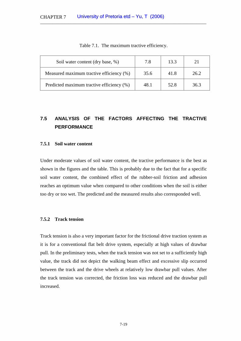
CHAPTER 7 __________________________________________________________________________________

Table 7.1. The maximum tractive efficiency.

Soil water content (dry base, %) 7.8 13.3 21

Measured maximum tractive efficiency (%) 35.6 41.8 26.2

Predicted maximum tractive efficiency (%) 48.1 52.8 36.3

7.5 ANALYSIS OF THE FACTORS AFFECTING THE TRACTIVE

PERFORMANCE

7.5.1 Soil water content

Under moderate values of soil water content, the tractive performance is the best as

shown in the figures and the table. This is probably due to the fact that for a specific

soil water content, the combined effect of the rubber-soil friction and adhesion

reaches an optimum value when compared to other conditions when the soil is either

too dry or too wet. The predicted and the measured results also corresponded well.

7.5.2 Track tension

Track tension is also a very important factor for the frictional drive traction system as

it is for a conventional flat belt drive system, especially at high values of drawbar

pull. In the preliminary tests, when the track tension was not set to a sufficiently high

value, the track did not depict the walking beam effect and excessive slip occurred

between the track and the drive wheels at relatively low drawbar pull values. After

the track tension was corrected, the friction loss was reduced and the drawbar pull

increased.

7-19


CHAPTER 7 __________________________________________________________________________________

7.5.3 Motion resistance and internal friction losses

The measured and predicted values of the motion resistances for three soil conditions

at different soil water content values are shown in Table 7.2. As can be seen, the

predicted and the measured motion resistance values depict large differences

probably caused by the internal frictional losses and the friction between the track

elements.

Table 7.2. Measured and predicted motion resistances.

Soil type Soil water content,

%, dry basis

Predicted external

motion resistance,

kN

Measured motion

resistance, kN

1 7.8 9.5 22.8

2 13.3 11.7 21.6

3 21 12.6 23.2

4 0, concrete surface - 12.8

The attention must be drawn to the fact that the measured motion resistance was

based on the input torque to the drive shaft and the predicted value by summation of

the horizontal force components below the track when the drawbar pull was zero. It

is proved that the internal resistance for all conditions was considerably higher than

expected.

7-20


CHAPTER 8 _____________________________________________________________________

CHAPTER VIII

SUMMARY, CONCLUSIONS AND RECOMMENDATIONS

8.1 SUMMARY

From the literature and the validation of the field tests and modelling undertaken in

this research, it was possible to develop an analytical model to predict the drawbar

performance for the prototype track based on the principles pioneered by Bekker and

other researchers. The proposed flexible track model was able to predict the contact

pressure distribution for a soft soil surface and therefore, also the frictional stress and

thrust force contributed by each track element.

Further more, the measurement and instrumentation system that was developed was

able to record the required soil parameters for the development of the analytical model.

Particularly, the rubber-soil friction was characterized by using a standard track

element and steel sinkage test plates.

Two force transducers were specially designed and built based on the theory of the

extended octagonal ring, to successfully measure the distribution of the contact

pressure and the friction-shear stress and thus the frictional force per track element.

A series of full-scale drawbar pull tests were conducted in the fields and the

relationships of traction and drawbar performance with total slippage under various

soil conditions were obtained.

The computerized data acquisition system was used to record all the in situ test results

for the soil characterization and the full-scale drawbar tests.

Through the modelling and the measurement, some design features of the prototype

traction system and the soil parameters were evaluated for their influence on the

8-1


CHAPTER 8 _____________________________________________________________________

tractive performance. These factors such as the frictional drive principle, the track

tension, the centre ground wheels and the soil water content played important roles for

the development of traction performance.

8.2 CONCLUSIONS

Based on the results from the field experiments and the performance prediction of the

analytical traction model, the following detailed conclusions were drawn:

1. The sinkage tests and the shear and frictional tests could be performed by the

instrumented test device. Related soil characteristics were obtained by

applying the processing procedure as required by the bevameter technique.

2. The contact pressure as recorded for all terrain conditions still displayed

typical peak values under the different wheels and the envisaged beam effect

did not materialize for the prototype track.

3. Wear and friction between steel track elements might be the major reason

causing the track to loose its initial bridging beam effect, resulting in an

increase in contact pressure under the driving and tension wheels.

4. As peak contact pressure still occurred, it proved that for the present it is not

justifiable to accept a uniform contact pressure distribution for the track as

envisaged by the inventor, thus omitting road wheels.

5. The track motion resistance was recorded as unacceptably high under all test

conditions, although the resistance on a concrete surface was considerably

lower than on soft surfaces. This appeared to be due to internal energy loss in

the track unit.

6. For the two models tested for predicting drawbar pull, i.e. a constant contact

pressure model, changing to trapezoidal and a flexible track model, with

typically undeformable truck wheels at the front and rear end and a circular

8-2


CHAPTER 8 _____________________________________________________________________

deflecting track section in between, the former proofed to be more idealized

and the later more practical.

7. For the deformable track model, reasonable agreement between the measured

and predicted values of contact pressure and traction force were observed for

individual traction elements.

8. The traction and drawbar pull coefficients of the prototype track, based on

measurements, were not as good as expected from modelling. In the criteria

for drawbar pull performance, the measured values were rather unacceptably

low when compared to results as reported in the other literature. This could

only be attributed to substantial internal energy losses for the tracks.

9. The tractive efficiency was also unacceptably low, apparently caused by high

internal friction between adjacent track elements and frictional slip between

the track and the driving wheels.

10. The soil water content influenced the soil characteristics and thus also the

traction performance of the tracks.

11. The research undertaken identified and confirmed a model to be used to

predict contact pressure and tangential stresses for a single track element.

12. By applying two octagonal ring transducers and other necessary test apparatus

and instrumentation, it was possible to measure the contact pressure and

tangential force on a single track element with minimal interference which was

confirmed by the predicted values.

13. Based on the proposed theoretical analysis, the tractive performance for

different possible contact pressure values could be predicted.

8-3


CHAPTER 8 _____________________________________________________________________

8.3 RECOMMENDATIONS

For possible future research, the following are recommendations, based on the results

from this study:

1. As the tractive performance of the tractor was not ideal as expected, it is

suggested that the complete operating principle of the walking beam concept

be reanalyzed and the source of the high internal losses be identified and

corrected.

2. The principle of an articulated beam track, with optimum traction

characteristics, was hampered by wear on the contact surfaces between

adjacent track elements. However, advantages offered by the tractor drive

train and steering system and the replacement of individual track elements

when damaged, justifies the development and testing of some effective means

to minimize friction and wear between track elements and sustain track tension

and the bridging effect.

3. Alternatively other available rubber covered steel tracks, with a positive drive

system, could be tested and combined with the novel steering and automatic

differential lock system.

4. The flexible track model, with the specific configuration of the contact profile,

was still not a universal model. To be applicable to new types of or modified

future tracks, the contact profile at the interface of the track and the terrain

surface may need to be observed and re-shaped.

5. Additional loading rollers or road wheels between the front and rear tension

and driving wheels could be added to achieve a more uniform distribution of

ground contact pressure under the tracks.

8-4


CHAPTER 8 _____________________________________________________________________

6. Based on the theoretical analysis, an optimum contact pressure distribution can

be proposed.

7. A modified track system based on the theoretical analysis is to be built and

tested and a modified model for tractive performance be tested.

8-5


LIST OF REFERENCES

ASAE, 1988. ASAE Standard S313.2. American Society of Agricultural Engineers,

St. Joseph, MI.

Barnard, J. H., 1989. United States Patent No. 4,882,947 dated November 28, 1989.

Track-laying device.

Bekker, M. G., 1956. Theory of Land Locomotion. University of Michigan Press,

Ann Arbor, MI.

Bekker, M. G., 1960. Off-the-road Locomotion. University of Michigan Press, Ann

Arbor, MI.

Bekker M. G., 1969. Introduction to Terrain-vehicle Systems. University of

Michigan Press, Ann Arbor, MI.

Caterpillar Inc., 1995. In pursuit of the ideal tractor – development of the rubber belt

tractor (ASAE distinguished lecture series, tractor design No. 20). Chicago, Illinois.

Chi, L., Tessier, S., McKyes, E. and Laguë, C., 1993. Modelling mechanical

behavior of agricultural soils. Transaction of the ASAE, 36 (6), pp. 1563-1570.

Chi, L., Kushwaha, R. L. and Shen, J., 1993. An elasto-plastic constitutive model for

agricultural cohesive soil. Canadian Agricultural Engineering, 35 (4), pp. 245-251.

Culshaw, D., 1988. Rubber tracks for traction. Journal of Terramechanics, 25 (1), pp.

69-80.

1


Dudzinksi, P. and Ketting, M., 1996. New hybrid friction/positive drive for rubber

belt running gear. Proceedings of the 12th International Conference of the ISTVS,

Beijing, China.

du Plessis, H.L.M., 1996. The Bi-Pole traction system-construction and performance.

Proceedings of the 12th International Conference of the ISTVS, Beijing, China.

du Plessis, H. L. M. and Yu, T., 1999. The tractive performance of a prototype track

based on rubber/soil friction and shear. Proceedings of the 13th International

Conference of the ISTVS, pp. 217-224. München, Germany.

Dwyer, M. J., Okello, J. A. and Scarlet, A. J., 1993. Theoretical and experimental

investigation of rubber tracks for agriculture. Journal of Terramechanics, 30 (4), pp.

285-298.

Evans, W. C. and Gove, D. S., 1986. Rubber belt track in agriculture. ASAE Paper

No.86-1061. St. Joseph, MI 49085-9659.

Esch, J. H., Bashford, L. L., Von Bargen, K. and Ekström, R. E., 1990. Tractive

performance comparisons between a rubber belt track and a four-wheel drive tractor.

Transactions of the ASAE, 36 (4), pp. 1563-1570.

Freitag, D. R., 1965. A dimensional analysis of the performance of pneumatic tires

on soft soils. Technical report No. 3-688, U.S. Army Engineers Waterways

Experiment Station, Vicksburg, Mississippi.

Girma, G., 1989. Multicomponent dynamometer for measurement of forces on

plough bodies. Journal of Agricultural Engineering Research, 42 (2), pp. 85-96.

Godwin, R. J., 1975. An extended octagonal ring transducer for use in tillage studies.

Journal of Agricultural Engineering Research, 20 (4), pp. 347-352.

2


Green, W. G., 1955. Theory of Machines. Blackie & Son Limited, London, pp. 674-

685.

Holm, C., Hefer, G. J. and Hintze, D., 1987. The influence of shape and size of a

penetration body on the pressure-sinkage relationship. Proceedings of the 9th

International Conference of the ISTVS. Barcelona, Spain.

Janosi, Z., Hanamoto, B., 1961. The analytical determination of drawbar pull as a

function of slip, for tracked vehicles in deformable soils. Proceedings of the 1st Int.

Conference Mech. Soil-Vehicle Systems. Turin, Italy.

Karafiath, L. L. and Nowatzki, E. A., 1978. Soil mechanics for off-road vehicle

engineering. Trans Tech Publications, Clausthal, Germany.

Koolen, A. J. and Kuipers, H., 1983. Agricultural Soil Mechanics. Springer-Verlag,

New York.

Lowen, E. G. and Cook, N. H., 1956. Metal cutting measurement and their

interaction. Experimental Stress Analysis, 13 (2), pp. 57-62.

McKyes, E. and Fan, T., 1985. Multiplate penetration tests to determine soil stiffness

moduli. Journal of Terramechanics, 22 (3), pp. 157-162.

McKyes, E., 1989. Agricultural Engineering Soil Mechanics (Developments in

Agricultural Engineering 10). Elsevier Science Publishers B.V., Amsterdam.

Neal, M.S., 1966. Friction and adhesion between soil and rubber. Journal of

Agricultural Engineering Research, 11 (2), pp. 108-112.

O’Dogherty, M. J., 1975. A dynamometer to measure the forces on a sugar beet.


3


O’Dogherty, M. J., 1996. The design of octagonal ring dynamometer. Journal of

Agricultural Engineering Research, 63 (1), pp. 9-18.

Okello, J. A., 1991. A Review of soil strength measurement techniques for prediction

of terrain vehicle performance. Journal of Agricultural Engineering Research, 50 (2),

pp. 129-155.

Okello, J. A., 1994. Prediction and experimental validation of the field tractive

performance of a rubber track unit. Journal of Agricultural Engineering Research, 59

(2), pp. 163-171.

Okello, J. A., Dwyer, M. J. and Cottrell, F. B., 1994. The tractive performance of

rubber tracks and a tractor driving wheel tyre as influenced by design parameters.


Okello, J. A., Watany, M. and Crolla, D. A., 1998. A theoretical and experimental

investigation of rubber track performance models. Journal of Agricultural

Engineering Research, 69 (1), pp. 15-24.

Reece, A. R., 1965-1966. Principles of soil-vehicle mechanics. Proc. Instn. Mech.

Engrs., 180, Part 2A(2), pp. 45-67.

Rula, A. A. and Nuttall, C. J., 1971. An analysis of ground mobility models

(ANAMOB). Technical Report M-71-4, U.S. Army Engineer Waterways Experiment

Station, Vicksburg, Mississippi.

Sela, A. D. and Ehrlich, I. R., 1972. Load support capability of flat plates of various

shapes in soil. Journal of Terramechanics, 8 (3), pp. 39-70.

Shen, J. and Kushwaha, R. L., 1998. Soil-machine interactions: a finite element

perspective. Marcel Dekker, New York.

4


Taylor, J. H. and Burt, E. C., 1973. Track and tire performance in agricultural soil.

Transaction of the ASAE, Vol. 18 (1), pp. 3-7.

Terzaghi, K., 1966. Theoretical Soil Mechanics. John Wiley & Sons, New York.

Thakur, T. C. and Godwin, R. J., 1988. Design of extended octagonal ring

dynamometer for rotary tillage studies. Agricultural Mechanization in Asia, Africa

and Latin America, 19 (3), pp. 23-28.

Turnage, G. W., 1972. Performance of soils under tire loads; Application of test

results to tire selection for off-road vehicles. Technical report No. 3-666, Report 8,

U.S. Army Engineers Waterways Experiment Station, Vicksburg, Mississippi.

Turnage, G. W., 1978. A synopsis of tire design and operational considerations

aimed at increasing in-soil tire drawbar performance. Proceedings of the 6th

International Conference of the ISTVS, Vol. II, pp. 757-810.

Upadhyaya, S. K., Wulfsohn, D. and Mehlschau, J., 1993. An instrumented device to

obtain traction related parameters. Journal of Terramechanics, 30 (1), pp. 1-20.

Upadayaya, S. K. and Wulfsohn, D., 1993. Traction prediction using soil parameters

obtained with an instrumented analog device. Journal of Terramechanics, 30 (2), pp.

85-100.

Wills, B. M. D., 1963. The measurement of soil shear strength and deformation

moduli and a comparison of the actual and theoretical performance of a family of

rigid tracks. Journal of Agricultural Engineering Research, 8 (2), pp. 115-131.

Wismer, R. D. and Luth, H. J., 1973. Off-road traction prediction for wheeled

vehicles. Journal of Terramechanics, 10 (2), pp. 49-61.

5


Wong, J. Y. and Reece, A. R., 1967. Prediction of rigid wheel performance based on

the analysis of soil-wheel stresses – Part II. Performance of towed rigid wheels.

Journal of Terramechanics, 4 (2), pp. 7-25.

Wong, J. Y., 1980. Data processing methodology in the characterization of the

mechanical properties of terrain. Journal of Terramechanics, 17 (1), pp. 13-41.

Wong, J. Y., 1989. Terramechanics and off-road vehicles. Elsevier Science

Publishers, B.V., Amsterdam.

Wong, J. Y., 1993. Theory of ground vehicles, 2nd Edition. John Wiley & Sons, Inc.,

New York.

Yong, R. N., Fattah, E. A. and Skiadas, N., 1984. Vehicle Traction Mechanics

(Developments in Agricultural Engineering 3). Elsevier Science Publishers B.V.,

Amsterdam.

Youssef, A. F. A. and Ali, G. A., 1982. Determination of soil parameters using plate

test. Journal of Terramechanics, 19 (2), pp. 129-148.

Yu, T., 1996. Measurement of soil characteristics for traction modelling under

African conditions. Proceedings of the 12th International Conference of the ISTVS,

Beijing, China.

Yu, T. and du Plessis, H. L. M., 1996. Extended octagonal ring transducers to measure

vertical and tangential forces between a track element of the bi-pole traction system

and the terrain. Agricultural Engineering in South Africa, 28 (1), pp. 32-40.

Yu, T. and du Plessis, H. L. M., 1997. Pressure distribution and frictional-shear stress

under a prototype crawler track. Agricultural Engineering in South Africa, 29 (1), pp.

79-87.

6


APPENDIX A

DRAWBAR PULL TEST RESULTS

0.0

10.0

20.0

30.0

40.0

50.0

60.0

70.0

0.00 0.10 0.20 0.30 0.40 0.50

Slip

Dra

wba

r pul

l (kN

)

0.00

0.10

0.20

0.30

0.40

0.50

Dra

wba

r coe

ffici

ent

Experimental result

Fitted data

Figure A1. Drawbar pull test results for soil water content 7.8% (dry basis), sandy

loam soil.

7


0.0

10.0

20.0

30.0

40.0

50.0

60.0

70.0

0.00 0.10 0.20 0.30 0.40 0.50

Slip

0.00

0.10

0.20

0.30

0.40

0.50

0.60

Dra

wba

r coe

ffici

ent

Figure A2. Drawbar pull test results for soil water content 13.3% (dry basis), sandy

loam soil.

Figure A3. Drawbar pull test results for soil water content 21% (dry basis), sandy loam soil.

Dra

wba

r pul

l (kN

)

Experimental resultFitted data

0.0

10.0

20.0

30.0

40.0

50.0

0.00 0.10 0.20 0.30 0.40 0.50

Slip

Dra

wba

r pul

l (kN

)

0.00

0.05

0.10

0.15

0.20

0.25

0.30

0.35

Dra

wba

r coe

ffici

ent

Experimental resultFitted data

8


Documents

THE TRACTIVE PERFORMANCE OF A FRICTION-BASED …