The Transform between Geographic Coordinates and … · The Transform between Geographic Coordinates and Location Codes of Aperture 4 Hexagonal Grid System Wang Ruia,*, Ben Jina,b,

The Transform between Geographic Coordinates and Location Codes of Aperture 4

Hexagonal Grid System

Wang Ruia,*, Ben Jina,b, Li Yalua, Du Lingyua

a Institute of Surveying and Mapping, Information Engineering University, Zhengzhou 450052, China- [email protected],

[email protected], [email protected], [email protected]

b State Key Laboratory of Resource and Environmental Information System, Chinese Academy of Science, Beijing 100101, China,

KEY WORDS: Discrete Global Grid System, Location Code, Geographic Coordinate, Conversion, Code Operation

ABSTRACT:

Discrete global grid system is a new data model which supports the fusion processing of multi-source geospatial data. In discrete

global grid systems, all cell operations can be completed by codes theoretically, but most of current spatial data are in the forms of

geographic coordinates and projected coordinates. It is necessary to study the transform between geographic coordinates and grid

codes, which will support data entering and getting out of the systems. This paper chooses the icosahedral hexagonal discrete global

system as a base, and builds the mapping relationships between the sphere and the icosahedron. Then an encoding scheme of planar

aperture 4 hexagonal grid system is designed and applied to the icosahedron. Basing on this, a new algorithm of transforms between

geographic coordinates and grid codes is designed. Finally, experiments test the accuracy and efficiency of this algorithm. The

efficiency of code addition of HLQT is about 5 times the efficiency of code addition of HQBS.

1. INTRODUCTION

Discrete Global Grid Systems (DGGS) is a new global-oriented

data model, of which the main characteristic is the digital

representation of geospatial location. DGGS partition the globe

into uniform grid cells in hierarchical structure and address

every cell using location code to substitute for traditional

geographic coordinates in operation. Compared with the

traditional spatial data models, DGGS take the globe as the

research object and provide worldwide uniform space datum.

Each grid cell is correspond to one geographical location and

cell size will change in terms of the level of grid, which help

process of multi-resource, isomerous and multi-resolution

geospatial data. Moreover, in DGGS, geometrical operation of

grid cells can be achieved completely by location codes which

improve efficiency of data computation and process.1

Common cell shapes used by DGGS are triangles, quadrangles

and hexagons. Compared with other two shapes, the topological

relationship of hexagonal grids is consistent, which is beneficial

* Corresponding author at: Information Engineering University,

Zhengzhou 450052, China

E-mail address: [email protected]

for spatial analysis like adjacency and connection (Sahr et al.,

2003; Ben et al., 2015a). Spatial sampling efficiency of

hexagonal grids is highest and helps data visualization (Sahr,

2011). The processing efficiency of sampling values is about 20

percent to 50 percent higher than quadrangles (Sahr, 2011).

In the regular polyhedral DGGS, the icosahedron has the most

face, hence its geometric distortion after projection is minimum.

Now, many researchers at home and abroad have made relevant

research into the icosahedral hexagonal discrete grid systems.

Sahr et al. (Sahr, 2005; Sahr, 2008) realized the fast indexing of

cells at different resolutions based on the Icosahedral Snyder

Equal Area aperture 3 Hexagonal grid (ISEA3H). Vince and

Zheng (Vince and Zheng, 2009) designed the algorithms of

location code operation and Fourier Transform of the

icosahedral aperture 3 hexagonal grid system. Tong et al.

(Tong , 2010; Tong et al., 2013) designed an indexing structure

called the Hexagonal Quad Balances Structure (HQBS). Ben et

al. (Ben et al., 2015a; Ben, 2005; Ben et al., 2007; Ben et al.,

2010; Ben et al., 2011; Ben et al., 2015b) researched into the

generation algorithm, code indexing and real-time display of

hexagonal DGGS. In engineering, PYXIS Innovation

The International Archives of the Photogrammetry, Remote Sensing and Spatial Information Sciences, Volume XLII-2/W7, 2017 ISPRS Geospatial Week 2017, 18–22 September 2017, Wuhan, China

This contribution has been peer-reviewed. https://doi.org/10.5194/isprs-archives-XLII-2-W7-161-2017 | © Authors 2017. CC BY 4.0 License.

161

mailto:[email protected]

mailto:[email protected]

Corporation in Canada developed the spatial data integration

software based on the ISEA3H grid system and its core

technology is PYXIS grid indexing patent (Peterson, 2006).

Although current research has made considerable progress,

some deficiency exists. In the PYXIS scheme, the direction of

grid cells will change with levels of resolution, which is not

beneficial to spatial analysis like adjacency. The concept model

of HQBS is so complicated that there are frequent failure in

code regularization and operaions will rollback, which seriously

affects computational efficiency. The operations of cells can

be completely realized by location code in grid systems, but at

present most spatial data are still represented and stored in the

form of traditional geographic coordinates or projection

coordinates. To ensure that spatial data can transform between

the traditional data organization framework and grid systems at

a high speed, it is necessary to make research on conversion

between geographic coordinates and location codes.

Above all, this paper chooses the icosahedral DGGS and firstly

establishes the mapping relationship between the regular

icosahedron and the sphere. Then, an encoding scheme of the

planar aperture 4 hexagonal grid system is designed and applied

into the icosahedron skillfully. Based on this, we desinged a

new algorithm of conversion between geographic coordinates

and location codes of grids and compares with the scheme

HQBS to verify validity and high efficicency of the algorithm.

2. LOCATION OF THE REGULAR ICOSAHEDRON

AND MAPPING RELAITON WITH THE SPHERE

In order to establish the mapping relation between the surface

of a regular icosahedron and the sphere, firstly we should

determine the location relationship between the regular

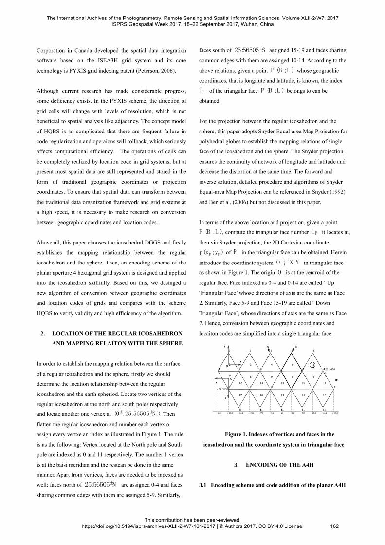
icosahedron and the earth spheriod. Locate two vertices of the

regular icosahedron at the north and south poles respectively

and locate another one vertex at (0±;25:56505±N ). Then

flatten the regular icosahedron and number each vertex or

assign every vertxe an index as illustrated in Figure 1. The rule

is as the following: Vertex located at the North pole and South

pole are indexed as 0 and 11 respectively. The number 1 vertex

is at the baisi meridian and the restcan be done in the same

manner. Apart from vertices, faces are needed to be indexed as

well: faces north of 25:56505±N are assigned 0-4 and faces

sharing common edges with them are assinged 5-9. Similarly,

faces south of 25:56505±S assigned 15-19 and faces sharing

common edges with them are assinged 10-14. According to the

above relations, given a point P (B ;L ) whose geograohic

coordinates, that is longitute and latitude, is known, the index

T P of the triangular face P (B ;L ) belongs to can be

obtained.

For the projection between the regular icosahedron and the

sphere, this paper adopts Snyder Equal-area Map Projection for

polyhedral globes to establish the mapping relations of single

face of the icosahedron and the sphere. The Snyder projection

ensures the continuity of network of longitude and latitude and

decrease the distortion at the same time. The forward and

inverse solution, detailed procedure and algorithms of Snyder

Equal-area Map Projection can be referenced in Snyder (1992)

and Ben et al. (2006) but not discussed in this paper.

In terms of the above location and projection, given a point

P (B ;L ), compute the triangular face number T P it locates at,

then via Snyder projection, the 2D Cartesian coordinate

p(xp;yp) of P in the triangular face can be obtained. Herein

introduce the coordinate system O ¡ X Y in triangular face

as shown in Figure 1. The origin O is at the centroid of the

regular face. Face indexed as 0-4 and 0-14 are called ‘ Up

Triangular Face’ whose directions of axis are the same as Face

2. Similarly, Face 5-9 and Face 15-19 are called ‘ Down

Triangular Face’, whose directions of axis are the same as Face

7. Hence, conversion between geographic coordinates and

locaiton codes are simplified into a single triangular face.

N

0 0 0 0

1111

144 ±180 - 144 - 108 -72 -36 0 36 72 108 144 ±180

11 11 11

0

4 5 1 2 3

8 9 10 6 7 8

3 4 0 1

6

10

5

14

9

13

8

12

7

17 18 19 15 16

3

N

26. 5650

5

-26. 56505

2

11

Y

X

X

Y

O

O

Figure 1. Indexes of vertices and faces in the

icosahedron and the coordinate system in triangular face

3. ENCODING OF THE A4H

3.1 Encoding scheme and code addition of the planar A4H



162

Above analysis, in order to complete the conversion, we need to

research relationship between locaiton codes on the triangular

faces and the correspongding 2D Cartesian coordinates. Centers

of grid cells are called lattice, which are identified with grid

cells in our research. For convnence of code substitution, this

paper adopts complex numbers to represent lattice locations

(Vince, 2006a, 2006b). Thereinaftet, let n denote the partition

level of grids, and the higher the level, the finer the resolution

or the size of grid cell. According to geometry of the aperture 4

hexagongal grid system (A4H), lattice at level n , n > 1,

comprises lattice and midpoints of each cell edges at level

n ¡ 1.

On the complex plane, let ! 0 =1

2+

p3

2i, D 0 = f0;! 0;! 02,

;! 03;! 04;! 05;! 06g , ! = ¡1

2+

p3

2i and D = f0;!;! 2 ,

;! 3g, the set of lattice of A4H is given by

8>><

>>:

L 1 =1

2D0

L n = L 1 +nP

i= 2

1

2iD

(1)

where ‘P

’ and ‘+’ mean accumulation among sets.

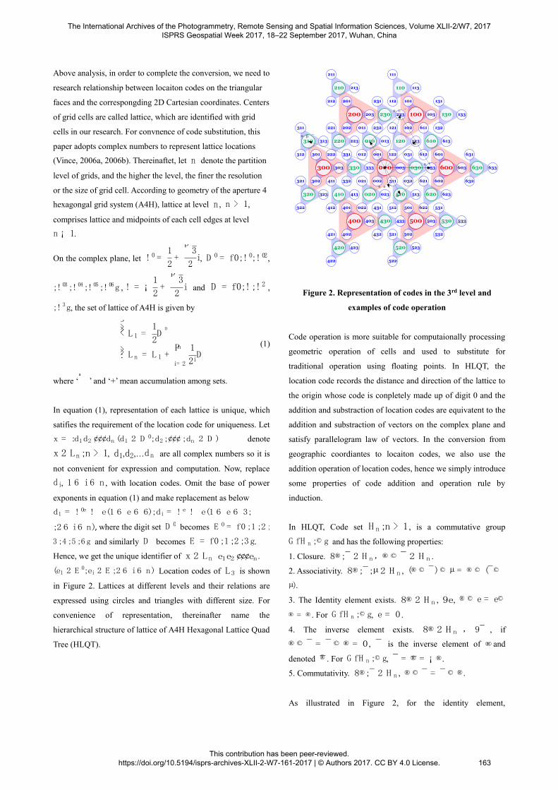
In equation (1), representation of each lattice is unique, which

satifies the requirement of the location code for uniqueness. Let

x = :d1d2 ¢¢¢dn (d1 2 D0;d2;¢¢¢;dn 2 D ) denote

x 2 Ln;n > 1, d1,d2,…dn are all complex numbers so it is

not convenient for expression and computation. Now, replace

di, 1 6 i6 n , with location codes. Omit the base of power

exponents in equation (1) and make replacement as below

d1 = !0e ! e(1 6 e 6 6);di = !

e ! e(1 6 e 6 3;

;2 6 i6 n), where the digit set D 0 becomes E 0 = f0 ;1 ;2 ;

3 ;4 ;5 ;6 g and similarly D becomes E = f0;1;2;3g.

Hence, we get the unique identifier of x 2 L n e1e2 ¢¢¢en .

(e1 2 E0;ei 2 E ;2 6 i6 n) Location codes of L3 is shown

in Figure 2. Lattices at different levels and their relations are

expressed using circles and triangles with different size. For

convenience of representation, thereinafter name the

hierarchical structure of lattice of A4H Hexagonal Lattice Quad

Tree (HLQT).

130

110

120

111

112

113

131

132

133

121

122

123

030

430

410

420

210

220

230

310

320

330

510

520

530

610

620

630

611

612

613

621

622

623

631

632

633

511

512

513

500

501

502

503

431

432

433

421

422

423

400

401

402

403

411

412

413

331

332

333

321

322

323

311

312

313

221

222

223

300

301

302

303 000

010

011

012

013

200

231

232

233

201

202

203

211

212

213

001

002

003

031

032

033 600

601

602

603

531

532

533

521

522

523

100

101

102

103

020

021

022

023

¯ ®

® © ¯

¯

® ª ¯

® Ð ¯

® ® ¯

Figure 2. Representation of codes in the 3rd level and

examples of code operation

Code operation is more suitable for computaionally processing

geometric operation of cells and used to substitute for

traditional operation using floating points. In HLQT, the

location code records the distance and direction of the lattice to

the origin whose code is conpletely made up of digit 0 and the

addition and substraction of location codes are equivatent to the

addition and substraction of vectors on the complex plane and

satisfy parallelogram law of vectors. In the conversion from

geographic coordiantes to locaiton codes, we also use the

addition operation of location codes, hence we simply introduce

some properties of code addition and operation rule by

induction.

In HLQT, Code set H n;n > 1 , is a commutative group

G fH n ;© g and has the following properties:

1. Closure. 8® ;̄ 2 H n，® © ¯ 2 H n .

2. Associativity. 8® ;̄ ;µ 2 H n , (® © ¯)© µ = ® © (̄ ©

µ).

3. The Identity element exists. 8® 2 H n , 9e, ® © e = e©

® = ® . For G fH n ;© g, e = 0 .

4. The inverse element exists. 8® 2 H n ， 9¯ , if

® © ¯ = ¯ © ® = 0 , ¯ is the inverse element of ® and

denoted ® . For G fH n ;© g, ¯ = ® = ¡ ® .

5. Commutativity. 8® ;̄ 2 H n , ® © ¯ = ¯ © ® .

As illustrated in Figure 2, for the identity element,



163

233 © 000 = 233 . For the inverse element, 010©

510 = 0;510 = 010 . For the property (5), 010 © 123 = .

123 © 010 = 233 . And these properties make G fH n ;© g

the Abelian group.The operation rule of code addtion is similar

to the decimal addition essentailly. In operation , we reference

the addition table as Table 1.

Table 1. Addition table of seven code cells

© 0 1 2 3 4 5 6

0 0 1 2 3 4 5 6

1 1 100 20 2 0 6 10

2 2 20 200 30 3 0 1

3 3 2 30 300 40 4 0

4 4 0 3 40 400 50 5

5 5 6 0 4 50 500 60

6 6 10 1 0 5 60 600

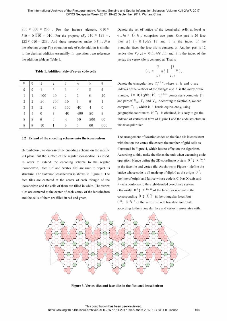
3.2 Extend of the encoding scheme onto the icosahedron

Hereinbefore, we discussed the encoding scheme on the infinite

2D plane, but the surface of the regular icosahedron is closed.

In order to extend the encoding scheme to the regular

icosahedron, ‘face tile’ and ‘vertex tile’ are used to depict its

structure. The flattened icosahedron is shown in Figure 3. The

face tiles are centered at the center of each triangle of the

icosahedron and the cells of them are filled in white. The vertex

tiles are centered at the center of each vertex of the icosahedron

and the cells of them are filled in red and green.

Denote the set of lattice of the icosahedral A4H at level n

G n (n > 1). G n comprises two parts. One part is 20 face

tiles A in ;i= 0;1;¢¢¢;19 and i is the index of the

triangular faces the face tile is centered at. Another part is 12

vertxe tiles V jn ;j = 0;1;¢¢¢;11 and j is the index of the

vertex the vertex tile is centered at. That is

G n =19[

i= 0

A in [11[

k= 0

V jn。

Denote the triangular face T a;b;ci , where a, b and c are

indexes of the vertices of the triangle and i is the index of the

triangle, i= 0;1;¢¢¢;19. T a;b;ci comprises a complete Pi

and part of Va , Vb and Vc. According to Section 2, we can

compute T P , which is i herein equivalently, using

geographic coordinates. If T P is obtained, it is easy to get the

indexed of vertices in term of Figure 1 and the code structure in

this triangular face.

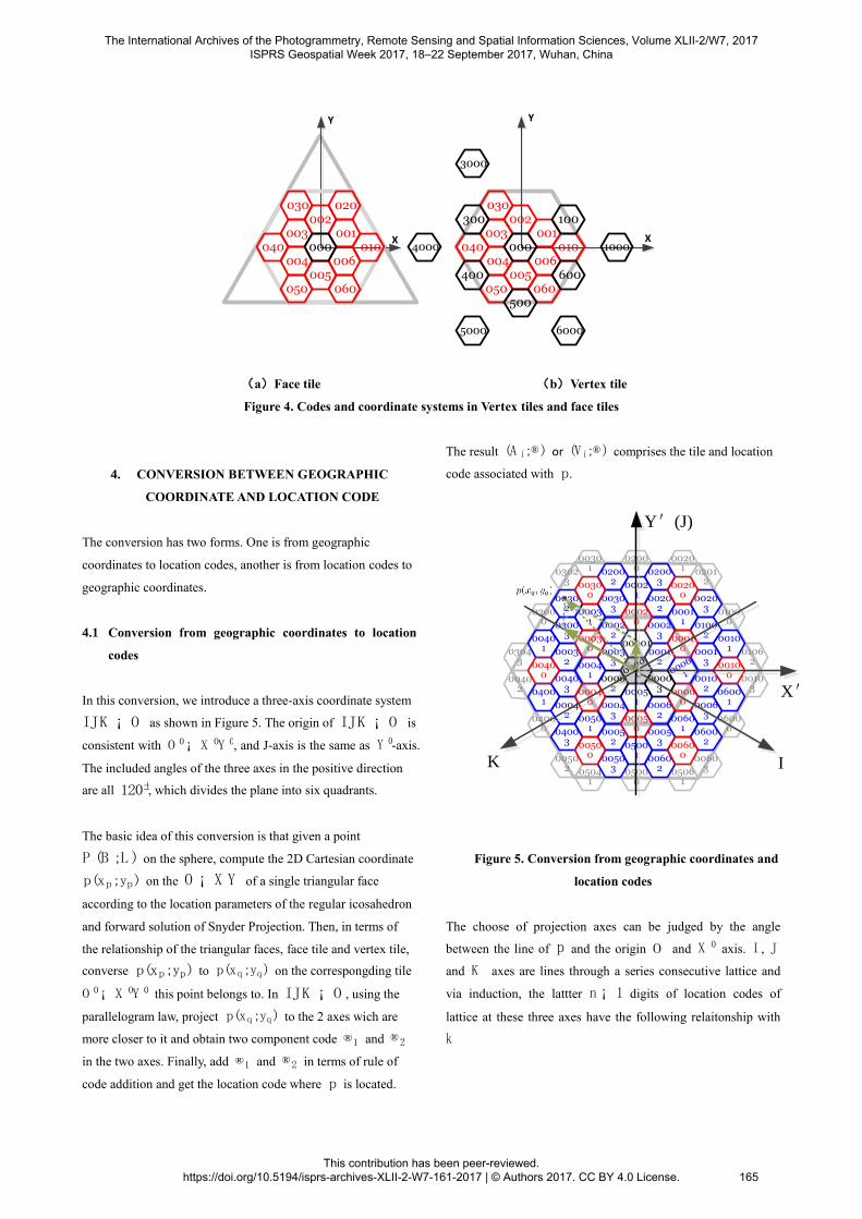
The arrangement of location codes on the face tile is consistent

with that on the vertex tile except the number of grid cells as

illustrated in Figure 4, which has no effect on the algorithm.

According to this, make the tile as the unit when executing code

operation. Hence define the 2D coordinate system O 0¡ X 0Y 0

in the face tile and vertex tile. As shown in Figure 4, define the

lattice whose code is all made up of digit 0 as the origin O 0,

the line of origin and lattice whose code is 010 as X-axis and

Y -axis conforms to the right-handed coordinate system.

Obviously, O 0¡ X 0Y 0 of the face tiles is equal to the

corresponding O ¡ X Y in the triangular faces, but

O 0¡ X 0Y 0 of the vertex tile will translate and rotate

according to the triangular face and vertex it associates with.

Figure 3. Vertex tiles and face tiles in the flattened icosahedron



164

X

Y Y

X001

020002

003040

030

050 060

006010

004005

000006

002003

004005

040

050 060

030

001010000

300

400

500

600

100

4000

5000

1000

6000

3000

（a）Face tile （b）Vertex tile

Figure 4. Codes and coordinate systems in Vertex tiles and face tiles

4. CONVERSION BETWEEN GEOGRAPHIC

COORDINATE AND LOCATION CODE

The conversion has two forms. One is from geographic

coordinates to location codes, another is from location codes to

geographic coordinates.

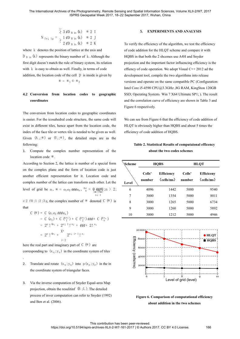
4.1 Conversion from geographic coordinates to location

codes

In this conversion, we introduce a three-axis coordinate system

IJK ¡ O as shown in Figure 5. The origin of IJK ¡ O is

consistent with O 0¡ X 0Y 0, and J-axis is the same as Y 0-axis.

The included angles of the three axes in the positive direction

are all 120±, which divides the plane into six quadrants.

The basic idea of this conversion is that given a point

P (B ;L ) on the sphere, compute the 2D Cartesian coordinate

p(xp;yp) on the O ¡ X Y of a single triangular face

according to the location parameters of the regular icosahedron

and forward solution of Snyder Projection. Then, in terms of

the relationship of the triangular faces, face tile and vertex tile,

converse p(xp;yp) to p(xq;yq) on the correspongding tile

O 0¡ X 0Y 0 this point belongs to. In IJK ¡ O , using the

parallelogram law, project p(xq;yq) to the 2 axes wich are

more closer to it and obtain two component code ®1 and ® 2

in the two axes. Finally, add ®1 and ® 2 in terms of rule of

code addition and get the location code where p is located.

The result (A i;®) or (Vi;® ) comprises the tile and location

code associated with p.

003010302

3

05041

00502

04000

00402

03043

03000

02000

00201 0201

2

01000

01062

00103

06000

006030506

105000

00022

00033

003030003

100011

00202

0006

1

00012

00023

00102

00013

00062 0060

100053

000510004

3

00052

00002

00041

00501

00032

0000

0

00021

03003

00042

05001

00063

01002

004030400

1

04003

00020

00030

00010

00060

00040

00050

00503

00500 0060

2

06001

060020060

0

00203

00101

00100

02002

02003 0020

000302

00300

00401

00400

00001

00003 X＇

K I

Y＇(J)

Figure 5. Conversion from geographic coordinates and

location codes

The choose of projection axes can be judged by the angle

between the line of p and the origin O and X 0 axis. I , J

and K axes are lines through a series consecutive lattice and

via induction, the lattter n ¡ 1 digits of location codes of

lattice at these three axes have the following relaitonship with

k



165

N fn ¡ 1g =

8><

>:

3 ¢D B in (k) ® 2 I

1 ¢D B in (k) ® 2 J

2 ¢D B in (k) ® 2 K

where k denotes the position of lattice at the axis and

D B in (k) represents the binary number of k . Although the

first digit doesn’t match the rule of binary system, its relation

with k is easy to obtain as well. Finally, in terms of code

addition, the location code of the cell p is inside is given by

® = ® 1 © ® 2

4.2 Conversion from location codes to geographic

coordinates

The conversion from location codes to geographic coordinates

is easier. For the icosahedral code structure, the same code will

exist in different tiles, hence apart from the location code, the

index of the face tile or vertex tile is needed to be given as well.

Given (A i;®) or (Vi;® ), the detailed steps are as the

following:

1. Compute the complex number representation of the

location code ® .

According to Section 2, the lattice is number of a special form

on the complex plane and the form of location code is just

another efficient representation for it. Location code and

complex number of the lattice can transform each other. Let the

level of grid be n , ® = e1e2 ¢¢¢en , ²en = 0 ¢¢¢0| {z }n ¡ 1

;n > 2;

e 2 f0 ;1 ;2 ;3 g, the complex number of ® denoted C (® ) is

that

C (®) = C (e1e2 ¢¢¢en )

= C (e1)+ C (²e21 )+ C (²

e22 )¢¢¢+ C (²

enn )

= 2n ! 0e1 + 2n ¡ 1! e2 + ¢¢¢+ 2! en

= 2n ! 0e1 +nX

i= 2

2n ¡ i+ 1! ei

here the real part and imaginary part of C (® ) are

corresponding to (xq;yq) in the coordinate system of tiles

.

2. Translate and rotate (xq;yq) into p(xp;yp) in the in

the coordinate system of triangular faces.

3. Via the inverse computation of Snyder Equal-area Map

projection, obtain the resulitinf (B ;L ). The detailed

process of inver computation can refer to Snyder (1992)

and Ben et al. (2006).

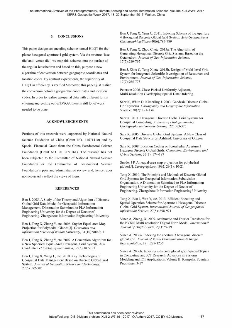
5. EXPERIMENTS AND ANALYSIS

To verify the efficiency of the algorithm, we test the efficiency

of code addition for the HLQT scheme and compare it with

HQBS in that both the 2 shcemes use A4H and Snyder

projection and the important factor influencing efficiency is the

effiency of code operation. We adopt Visual C++ 2012 ad the

development tool, compile the two algorithms into release

versions and operate on the same compatible PC (Configuration:

Intel Core i5-4590 [email protected] ,8G RAM, KingSton 120GB

SSD; Operating System：Win 7 X64 Ultimate SP1; ). The result

and the correlation curve of efficiency are shown in Table 3 and

Figure 6 respectively.

We can see from Figure 6 that the efficiency of code addition of

HLQT is obviously higher than HQBS and about 5 times the

efficiency of code addition of HQBS.

Table 2. Statistical Results of computaional efficency

about the two codes schemes

Scheme

Level

HQBS HLQT

Cells’

number

Efficiency

（cells/ms）

Cells’

number

Efficiceny

（cells/ms）

6 4096 1442 5000 9540

7 3000 1354 5000 8011

8 3000 1265 5000 6734

9 3000 1260 5000 5892

10 3000 1212 5000 4946

HQBS

HLQT

Level of grid (level)

Effic

ien

cy (c

ells

/ms)

Figure 6. Comparison of computational efficiency

about addition in the two schemes



166

mailto:i5-4590%[email protected]

6. CONCLUSIONS

This paper designs an encoding scheme named HLQT for the

planar hexagonal aperture 4 grid system. Via the struture ‘face

tile’ and ‘vertec tile’, we map this scheme onto the surface of

the regular icosahedron and based on this, purpose a new

algorithm of conversion between geographic coordinates and

location codes. By contrast experiments, the superiority of

HLQT in efficiency is verified.Moreover, this paper just realize

the conversion between geographic coordinates and location

codes. In order to realize geospatial data with different forms

entering and getting out of DGGS, there is still lot of work

needed to be done.

ACKNOWLEDGEMENTS

Portions of this research were supported by National Natural

Science Foudation of China (Grant NO. 41671410) and by

Special Financial Grant from the China Postdoctoral Science

Foundation (Grant NO. 2013T60161). The research has not

been subjected to the Committee of National Natural Science

Foundation or the Committee of Postdoctoral Science

Foundation’s peer and administrative review and, hence, does

not necessarily reflect the views of them.

REFERENCES

Ben J. 2005. A Study of the Theory and Algorithm of Discrete

Global Grid Data Model for Geospatial Information

Management. Dissertation Submitted to PLA Information

Engineering University for the Degree of Doctor of

Engineering. Zhengzhou: Information Engineering University

Ben J, Tong X, Zhang Y, etc. 2006. Snyder Equal-area Map

Projection for Polyhedral Globes[J]. Geomatics and

Information Science of Wuhan University, 31(10):900-903

Ben J, Tong X, Zhang Y, etc. 2007. A Generation Algorithm for

a New Spherical Equal-Area Hexagonal Grid System. Acta

Geodaetica et Cartographica Sinica, 36(5):187-191

Ben J, Tong X, Wang L, etc. 2010. Key Technologies of

Geospatial Data Management Based on Discrete Global Grid

System. Journal of Geomatics Science and Technology,

27(5):382-386

Ben J, Tong X, Yuan C. 2011. Indexing Schema of the Aperture

4 Hexagonal Discrete Global Grid System. Acta Geodaetica et

Cartographica Sinica,40(6):785-789

Ben J, Tong X, Zhou C, etc. 2015a. The Algorithm of

Generating Hexagonal Discrete Grid Systems Based on the

Octahedron. Journal of Geo-Information Science.

17(7):789-797

Ben J, Zhou C, Tong X, etc. 2015b. Design of Multi-level Grid

System for Integrated Scientific Investigation of Resources and

Environment. Journal of Geo-Information Science,

17(7):765-773

Peterson 2006. Close-Packed Uniformly Adjacent,

Multi-resolution Overlapping Spatial Data Ordering.

Sahr K, White D, Kimerling J. 2003. Geodesic Discrete Global

Grid Systems. Cartography and Geographic Information

Science, 30(2): 121-134

Sahr K. 2011. Hexagonal Discrete Global Grid Systems for

Geospatial Computing. Archives of Photogrammetry,

Cartography and Remote Sensing, 22: 363-376

Sahr K. 2005. Discrete Global Grid Systems: A New Class of

Geospatial Data Structures. Ashland: University of Oregon

Sahr K. 2008. Location Coding on Icosahedral Aperture 3

Hexagon Discrete Global Grids. Computers, Environment and

Urban Systems, 32(3): 174-187

Snyder J P. An equal-area map projection for polyhedral

globes[J]. Cartographica, 1992, 29(1): 10-21

Tong X. 2010. The Principle and Methods of Discrete Global

Grid Systems for Geospatial Information Subdivision

Organization. A Dissertation Submitted to PLA Information

Engineering University for the Degree of Doctor of

Engineering. Zhengzhou: Information Engineering University

Tong X, Ben J, Wan Y, etc. 2013. Efficient Encoding and

Spatial Operation Scheme for Aperture 4 Hexagonal Discrete

Global Grid System. International Journal of Geographical

Information Science, 27(5): 898-921

Vince A, Zheng, X. 2009. Arithmetic and Fourier Transform for

the PYXIS Multi-resolution Digital Earth Model. International

Journal of Digital Earth, 2(1): 59-79

Vince A, 2006a. Indexing the aperture 3 hexagonal discrete

global grid. Journal of Visual Communication & Image

Representation, 17: 1227-1236

Vince A, 2006b. Indexing a discrete global grid. Special Topics

in Computing and ICT Research, Advances in Systems

Modeling and ICT Applications, Volume II. Kampala: Fountain

Publishers. 3-17



167

Documents

The Transform between Geographic Coordinates and … · The Transform between Geographic Coordinates and Location Codes of Aperture 4 Hexagonal Grid System Wang Ruia,*, Ben Jina,b,