THE TRANSMUTED BIRNBAUM–SAUNDERS DISTRIBUTION · (vi) its scale parameter is also its median, so that the BS distribution can be seen as an analogue, but in an asymmetrical setting,

REVSTAT – Statistical Journal

Volume 15, Number 4, October 2017, 601–628

THE TRANSMUTED BIRNBAUM–SAUNDERS

DISTRIBUTION

Authors: Marcelo Bourguignon

– Department of Statistics, Universidade Federal do Rio Grande do Norte,[email protected]

Jeremias Leao

– Department of Statistics, Universidade Federal do Amazonas,[email protected]

Vıctor Leiva

– School of Industrial Engineering, Pontificia Universidad Catolica de Valparaıso,[email protected], www.victorleiva.cl

Manoel Santos-Neto

– Department of Statistics, Universidade Federal de Campina Grande,[email protected], www.santosnetoce.com.br

Received: February 2016 Revised: April 2016 Accepted: April 2016

Abstract:

• The Birnbaum–Saunders distribution has been largely studied and applied becauseof its attractive properties. We introduce a transmuted version of this distribution.Various of its mathematical and statistical features are derived. We use the maximumlikelihood method for estimating its parameters and determine the score vector andHessian matrix for inference and diagnostic purposes. We evaluate the performanceof the maximum likelihood estimators by a Monte Carlo study. We illustrate the po-tential applications of the new transmuted Birnbaum–Saunders distribution by meansof three real-world data sets from different areas.

Key-Words:

• data analysis; likelihood methods; Monte Carlo simulations; Ox and R softwares;

transmutation map.

AMS Subject Classification:

• 62F10; 62J20; 62P99.

602 M. Bourguignon, J. Leao, V. Leiva and M. Santos-Neto

The Transmuted Birnbaum–Saunders Distribution 603

1. INTRODUCTION

The Birnbaum–Saunders (BS) distribution has been widely studied and

applied due to its interesting properties. Some of its more relevant characteristics

are the following:

(i) it is a transformation of the normal distribution, inheriting several of

its properties;

(ii) it has two parameters, modifying its shape and scale;

(iii) it has positive skewness, doing its probability density function (PDF)

to be asymmetrical to the right, but due to its flexibility, symmetric

data can also be modeled by the BS distribution;

(iv) its PDF and failure rate (FR) are unimodal, but also other shapes

for its FR may be modeled;

(v) it belongs to the scale and closed under reciprocation families of dis-

tributions; and

(vi) its scale parameter is also its median, so that the BS distribution can

be seen as an analogue, but in an asymmetrical setting, of the normal

distribution, which has the mean as one of its parameters.

For more details of the BS distribution, see Birnbaum and Saunders (1969b),

Johnson et al. (1995, pp. 651–663), or the recent book by Leiva (2016). The

BS distribution is a direct competitor of the gamma, inverse Gaussian (IG),

lognormal and Weibull distributions; see details of these last distributions in

Johnson et al. (1994).

The BS distribution has its genesis from fatigue of materials. Then, its

natural applications have been mainly focussed on engineering and reliability.

However, today they range diverse fields including business, environment and

medicine. For some of its more recent applications, see Villegas et al. (2011),

Marchant et al. (2013, 2016a,b), Saulo et al. (2013, 2017), Leiva et al. (2014a,d,

2015a, 2016c, 2015b, 2017), Rojas et al. (2015), Wanke and Leiva (2015), Desousa

et al. (2017), Garcia-Papani et al. (2017), Leao et al. (2017a,b), Lillo et al. (2016)

and Mohammadi et al. (2017). These and other applications, as well as several

extensions and generalizations of the BS distribution, have been conducted by an

international, transdisciplinary group of researchers. The first extension of the BS

distribution is attributed to Volodin and Dzhungurova (2000), which established

that the BS distribution is the mixture equally weighted of an IG distribution

and its convolution with the chi-squared distribution with one degree of freedom.

The authors provided a physical interpretation in terms of fatigue-life models

and introduced a general family of distributions, with members such as the IG,

normal and BS distributions, as well as others used in reliability applications.

Then, Dıaz-Garcıa and Leiva (2005) introduced the generalized BS (GBS) distri-

bution; see also Azevedo et al. (2012). Owen (2006) proposed a three-parameter


extension of the BS distribution. Vilca and Leiva (2006) derived a BS distribution

based on skew-normal models (skew-BS). Gomez et al. (2009) extended the BS

distribution from the slash-elliptic model. Guiraud et al. (2009) deducted a non-

central version of the BS distribution. Leiva et al. (2009) provided a length-biased

version of the BS distribution. Ahmed et al. (2010) analyzed a truncated version

of the BS distribution. Kotz et al. (2010) performed mixture models related to

the BS distribution. Vilca et al. (2010) and Castillo et al. (2011) developed the

epsilon-skew BS distribution. Balakrishnan et al. (2011) considered mixture BS

distributions. Cordeiro and Lemonte (2011) defined the beta-BS distribution.

Leiva et al. (2011) modeled wind energy flux using a shifted BS distribution.

Athayde et al. (2012) viewed the BS distributions as part of the Johnson system,

allowing location-scale BS distributions to be obtained. Ferreira et al. (2012) and

Leiva et al. (2016a) proposed an extreme value version of the BS distribution

and its modeling. Santos-Neto et al. (2012, 2014, 2016) and Leiva et al. (2014c)

reparameterized the BS distribution obtaining interesting properties and mod-

eling. Saulo et al. (2012) presented the Kumaraswamy-BS distribution. Fierro

et al. (2013) generated the BS distribution from a non-homogeneous Poisson

process. Lemonte (2013) studied the Marshall–Olkin-BS (MOBS) distribution.

Bourguignon et al. (2014) derived the power-series BS class of distributions. Mar-

tinez et al. (2014) introduced an alpha-power extension of the BS distribution.

Leiva et al. (2016c) derived a zero-adjusted BS distribution.

The above mentioned review about extensions and generalizations of the

BS distribution is in agreement with the important growing that the distribution

theory has had in the last decades. This is because, although the Gaussian (or

normal) distribution has dominated this theory during more than 100 years, many

real-world applications cannot be well modeled by this distribution. Then, non-

normal distributions which must be flexible in skewness and kurtosis are needed.

The interested reader can find a good collection of non-normal distributions in

Johnson et al. (1994, 1995). Several of these distributions were constructed us-

ing methods early proposed by Pearson (1895), Edgeworth (1917), Cornish and

Fisher (1937) and Johnson (1949), based on differential equations, mathematical

approximations and translation techniques; see more details in Johnson et al.

(1994, pp. 15–62). A more recent proposal on non-normal distributions is at-

tributed to Azzalini (1985). In the line of these works and motivated from fi-

nancial mathematics, where applications in the calculation of value at risk and

corrections to the Black–Scholes options need flexibility in skewness and kurto-

sis, Shaw and Buckley (2009) introduced new parametric families of distributions

based on the transmutation method. This method modifies the skewness and/or

kurtosis into symmetric and asymmetric distributions and generates a new dis-

tributional family known as transmuted (or changed in its shape) distributions.

The transmutation method proposed by Shaw and Buckley (2009) carries out a

function composition between the cumulative distribution function (CDF) of a

distribution and the quantile function (QF) of another. Aryal and Tsokos (2009)


defined the transmuted extreme value distribution. Aryal and Tsokos (2011) and

Khan and King (2013) presented transmuted Weibull distributions. Aryal (2013)

proposed the transmuted log-logistic distribution. Ashour and Eltehiwy (2013)

analyzed the transmuted Lomax distribution. Mroz (2013a,b) studied the trans-

muted Lindley and Rayleigh distributions, whereas Sharma et al. (2014) derived

a transmuted inverse Rayleigh distribution. Khan and King (2014) considered

the transmuted inverse Weibull distribution. Merovci and Puka (2014) deduced

the transmuted Pareto distribution. Tiana et al. (2014) developed the trans-

muted linear exponential distribution. Saboor et al. (2015) created a transmuted

exponential-Weibull distribution. Louzada and Granzotto (2016) introduced the

transmuted log-logistic regression model. To our best knowledge, no transmuted

versions of the BS distribution exist. Therefore, the main objective of this pa-

per is to propose and derive the transmuted BS (TBS) distribution, as well as a

comprehensive treatment of its mathematical and statistical properties.

Section 2 presents the TBS distribution and derives some of its characteris-

tics including its PDF, CDF and QF, as well as its FR, moments and a generator

of random numbers. Section 3 provides the estimation of the TBS parameters

using the maximum likelihood (ML) method, including the corresponding score

vector and Hessian matrix for inferential and diagnostic purposes. In this sec-

tion, the performance of the ML estimators is evaluated by means of Monte Carlo

(MC) simulations. In addition, diagnostic tools are derived to detect influential

data in the ML estimation. Section 4 illustrates the potential applications of the

TBS distribution with three real-world data sets from different areas. Section 5

discusses the conclusions of this work and future research about the topic.

2. FORMULATION AND CHARACTERISTICS

In this section, we provide a background of the BS distribution, formulate

the new distribution and obtain some of its more relevant characteristics.

2.1. The BS distribution

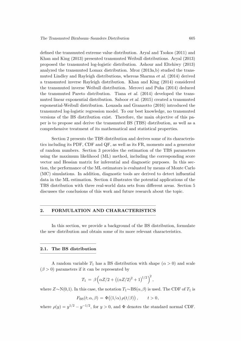
A random variable T1 has a BS distribution with shape (α > 0) and scale

(β > 0) parameters if it can be represented by

T1 = β(αZ/2 +

((αZ/2)2 + 1

)1/2)2

,

where Z∼N(0,1). In this case, the notation T1∼BS(α,β) is used. The CDF of T1 is

FBS(t; α, β) = Φ((1/α) ρ(t/β)

), t > 0,

where ρ(y) = y1/2 − y−1/2, for y > 0, and Φ denotes the standard normal CDF.


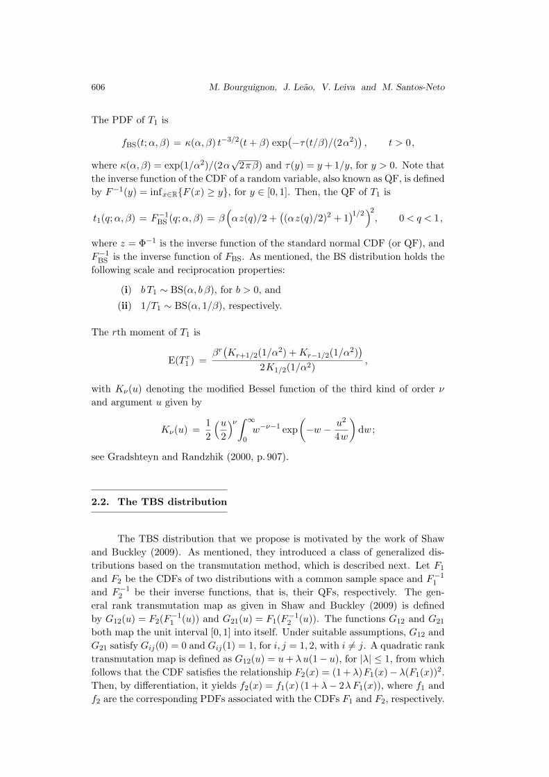
The PDF of T1 is

fBS(t; α, β) = κ(α, β) t−3/2(t + β) exp(−τ(t/β)/(2α2)

), t > 0,

where κ(α, β) = exp(1/α2)/(2α√

2πβ) and τ(y) = y + 1/y, for y > 0. Note that

the inverse function of the CDF of a random variable, also known as QF, is defined

by F−1(y) = infx∈RF (x) ≥ y, for y ∈ [0, 1]. Then, the QF of T1 is

t1(q; α, β) = F−1BS (q; α, β) = β

(αz(q)/2 +

((αz(q)/2)2 + 1

)1/2)2

, 0 < q < 1,

where z = Φ−1 is the inverse function of the standard normal CDF (or QF), and

F−1BS is the inverse function of FBS. As mentioned, the BS distribution holds the

following scale and reciprocation properties:

(i) b T1 ∼ BS(α, b β), for b > 0, and

(ii) 1/T1 ∼ BS(α, 1/β), respectively.

The rth moment of T1 is

E(T r1 ) =

βr(Kr+1/2(1/α2) + Kr−1/2(1/α2)

)

2K1/2(1/α2),

with Kν(u) denoting the modified Bessel function of the third kind of order ν

and argument u given by

Kν(u) =1

2

(u

2

)ν∫

∞

0w−ν−1 exp

(−w − u2

4w

)dw ;

see Gradshteyn and Randzhik (2000, p. 907).

2.2. The TBS distribution

The TBS distribution that we propose is motivated by the work of Shaw

and Buckley (2009). As mentioned, they introduced a class of generalized dis-

tributions based on the transmutation method, which is described next. Let F1

and F2 be the CDFs of two distributions with a common sample space and F−11

and F−12 be their inverse functions, that is, their QFs, respectively. The gen-

eral rank transmutation map as given in Shaw and Buckley (2009) is defined

by G12(u) = F2(F−11 (u)) and G21(u) = F1(F

−12 (u)). The functions G12 and G21

both map the unit interval [0, 1] into itself. Under suitable assumptions, G12 and

G21 satisfy Gij(0) = 0 and Gij(1) = 1, for i, j = 1, 2, with i 6= j. A quadratic rank

transmutation map is defined as G12(u) = u + λ u(1− u), for |λ| ≤ 1, from which

follows that the CDF satisfies the relationship F2(x) = (1 + λ)F1(x)− λ(F1(x))2.

Then, by differentiation, it yields f2(x) = f1(x) (1 + λ− 2λ F1(x)), where f1 and

f2 are the corresponding PDFs associated with the CDFs F1 and F2, respectively.


For more details about the quadratic rank transmutation map, see Shaw and

Buckley (2009). By using the BS CDF and PDF, we have the TBS CDF and

PDF, with parameters α, β and λ, given respectively by

FTBS(t; α, β, λ) = (1 + λ)Φ((1/α) ρ(t/β)

)− λ

(Φ((1/α) ρ(t/β)

))2,

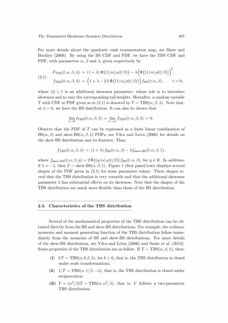
(2.1)fTBS(t; α, β, λ) =

(1 + λ − 2λ Φ

((1/α) ρ(t/β)

))fBS(t; α, β), t > 0,

where |λ| ≤ 1 is an additional skewness parameter, whose role is to introduce

skewness and to vary the corresponding tail weights. Hereafter, a random variable

T with CDF or PDF given as in (2.1) is denoted by T ∼ TBS(α, β, λ). Note that,

at λ = 0, we have the BS distribution. It can also be shown that

limt→0

fTBS(t; α, β, λ) = limt→∞

fTBS(t; α, β, λ) = 0 .

Observe that the PDF of T can be expressed as a finite linear combination of

BS(α, β) and skew-BS(α, β, 1) PDFs; see Vilca and Leiva (2006) for details on

the skew-BS distribution and its features. Thus,

fTBS(t; α, β, λ) = (1 + λ) fBS(t; α, β) − λfskew-BS(t; α, β, 1),

where fskew-BS(t; α, β, η) = 2 Φ((η/α) ρ(t/β)

)fBS(t; α, β), for η ∈ R. In addition,

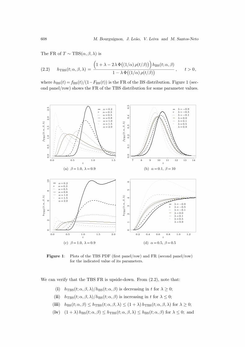
if λ = −1, then T ∼ skew-BS(α, β, 1). Figure 1 (first panel/row) displays several

shapes of the PDF given in (2.1) for some parameter values. These shapes re-

veal that the TBS distribution is very versatile and that the additional skewness

parameter λ has substantial effects on its skewness. Note that the shapes of the

TBS distribution are much more flexible than those of the BS distribution.

2.3. Characteristics of the TBS distribution

Several of the mathematical properties of the TBS distribution can be ob-

tained directly from the BS and skew-BS distributions. For example, the ordinary

moments and moment generating function of the TBS distribution follow imme-

diately from the moments of BS and skew-BS distributions. For more details

of the skew-BS distribution, see Vilca and Leiva (2006) and Saulo et al. (2013).

Some properties of the TBS distribution are as follow. If T ∼ TBS(α, β, λ), then:

(i) b T ∼ TBS(α, b β, λ), for b > 0, that is, the TBS distribution is closed

under scale transformations;

(ii) 1/T ∼ TBS(α, 1/β,−λ), that is, the TBS distribution is closed under

reciprocation;

(iii) Y = (α2/β)T ∼ TBS(α, α2, λ), that is, Y follows a two-parameter

TBS distribution.


The FR of T ∼ TBS(α, β, λ) is

(2.2) hTBS(t; α, β, λ) =

(1 + λ − 2λ Φ

((1/α) ρ(t/β)

))hBS(t; α, β)

1 − λ Φ((1/α) ρ(t/β)

) , t > 0,

where hBS(t) = fBS(t)/(1−FBS(t)) is the FR of the BS distribution. Figure 1 (sec-

ond panel/row) shows the FR of the TBS distribution for some parameter values.

t

fT

BS(t

;α

,β

,λ)

0.0

0.0

0.5

0.5

1.0

1.0

1.5

1.5

2.0

2.5 α =0.2

α =0.3α =0.5α =0.8α =1.0α =1.5α =2.0

(a) β = 1.0, λ = 0.9

t

fT

BS(t

;α

,β

,λ)

λ =0.0

0.0

0.5

0.2

0.4

0.1

0.3

7 8 9 10 11 12 13 14

λ =−0.9λ =−0.5λ =−0.1

λ =0.1λ =0.5λ =0.9

(b) α = 0.1, β = 10

t

hT

BS(t

;α

,β

,λ)

0.0 0.5 1.0 1.5 2.0

02

46

810

α =0.2α =0.3α =0.5α =0.8α =1.0α =1.5α =2.0

(c) β = 1.0, λ = 0.9

t

λ =0.0

hT

BS(t

;α

,β

,λ)

1.00.2 0.4

01

23

45

6

0.6 0.8 1.2

λ =−0.9λ =−0.5λ =−0.1

λ =0.1λ =0.5λ =0.9

(d) α = 0.5, β = 0.5

Figure 1: Plots of the TBS PDF (first panel/row) and FR (second panel/row)for the indicated value of its parameters.

We can verify that the TBS FR is upside-down. From (2.2), note that:

(i) hTBS(t; α, β, λ)/hBS(t; α, β) is decreasing in t for λ ≥ 0;

(ii) hTBS(t; α, β, λ)/hBS(t; α, β) is increasing in t for λ ≤ 0;

(iii) hBS(t; α, β) ≤ hTBS(t; α, β, λ) ≤ (1 + λ)hTBS(t; α, β, λ) for λ ≥ 0;

(iv) (1 + λ)hBS(t; α, β) ≤ hTBS(t; α, β, λ) ≤ hBS(t; α, β) for λ ≤ 0; and


(v) limt→0 hTBS(t; α, β, λ) = 0 and limt→∞ hTBS(t; α, β, λ) = 1/(2α2β),

that is, the limiting behaviors of the FRs of the TBS and BS dis-

tributions are the same.

Observe that the expression given in (2.2) may also be written as

hTBS(t; α, β, λ) = p(t)hBS(t; α, β) +(1 − p(t)

)hskew-BS(t; α, β, 1),

where p(t) =((1 + λ)

(1 − Φ

((1/α) ρ(t/β)

)))/(1 − (1 + λ)Φ

((1/α) ρ(t/β)

)+

λ(Φ((1/α) ρ(t/β)

))2), whereas hBS and hskew-BS are the FRs of the BS and

skew-BS distributions, respectively.

Many important features of a distribution can be obtained through its moments.

Let T1 ∼ BS(α, β) and T2 ∼ skew-BS(α, β, 1). Then, their rth moments are

E(T r1 ) =

βrα2 r

23r−1

r∑

k=0

k∑

i=0

(2 r

2 k

)(k

i

)(α2

4

)i−k

,(2.3)

E(T r2 ) = βr

r∑

k=0

k∑

i=0

(r

k

)(k

i

)2i(α

2

)k+1wk+1;k−i , r = 1, 2, ... ,(2.4)

where wa,b=E(Za(

√α2Z2+4)b

)and Z∼ skew-normal(0, 1, 1); see Azzalini (1985).

The rth moment of T ∼ TBS(α, β, λ) can be written as E(T r) = (1 + λ) E(T r1 )−

λE(T r2 ). Then, using the results presented in (2.3) and (2.4), we obtain

E(T r) = βr

r∑

k=0

k∑

j=0

((1 + λ)

(2 r

2 k

)(k

j

)α2(r−k+j)

23(r−k+j)−1

−λ

(r

k

)(k

j

)2j(α

2

)k+1wk+1;k−j

) .

Therefore, the first four moments of T ∼ TBS(α, β, λ) are

E(T ) = µ = β

(1 +

α2

2

)(1 + λ − λ

(1 +

α w1,1

(2 + α2)

)),

E(T 2) = β2

(1 + 2α2 +

3

2α4

)(1 + λ − λ

(1 +

2 α w1,1 + α3w3,1

2 + 4α2 + 3α4

)),

E(T 3) = β3

(1 +

9

2α2 + 9α4 +

15

2α6

)

×(

1 + λ − λ

(1 +

3 α w1,1 + 4α3w3,1 + α5w5,1

2 + 9α2 + 18α4 + 15α6

)),

E(T 4) = β4

(1 + 8α2 + 30α4 + 60α6 +

105

2α8

)

×(

1 + λ − λ

(1 +

4 α w1,1 + 10α3w3,1 + 6α5w5,1 + α7w7,1

2 + 16α2 + 60α4 + 120α6 + 105α8

)).


Thus, the rth moment of T ∼ TBS(α, β, λ) about its mean is

E((T − µ)r

)= (1 + λ)

r∑

j=0

(r

j

)(µ1 − µ)r−j E

((T1 − µ1)

j)

−λr∑

j=0

(r

j

)(µ2 − µ)r−j E

((T2 − µ2)

j),

where µ1 = β(1 + α2/2

)and µ2 = β

(1 + α w1,1 + α2/2

). Hence, the correspond-

ing second, third and fourth moments about the mean are

E((T − µ)2

)= Var(T ) = (1 + λ)

((µ1 − µ)2 + σ2

1

)− λ

((µ2 − µ)2 + σ2

2

),

E((T − µ)3

)= (1 + λ)

((µ1 − µ)3 + 3σ2

1 + µ(3)1

)− λ

((µ2 − µ)3 + 3σ2

2 + µ(3)2

),

E((T − µ)4

)= (1 + λ)

((µ1 − µ)4 + 6(µ1 − µ)2σ2

1 + 6(µ1 − µ)µ(3)1 + µ

(4)1

)

−λ((µ2 − µ)4 + 6(µ2 − µ)2σ2

2 + 6(µ1 − µ)µ(3)2 + µ

(4)2

),

where

σ21 = Var(T1) = α2β2

(1 + (5/4)α2

),

σ22 = Var(T2) = (β2/4)

(4 α2 − α2w2

1,1 + 2α3w3,1 − 2 α3w1,1 + 5α4),

µ(3)1 = β3α4

(3 + (11/2)α2

),

µ(4)1 = β4α4

(3 + (45/2)α2 + (633/16)α4

),

µ(3)2 = µ

(3)1 + (α3β3/4)

(2 α2w5,1 + 2w3,1 − 3 α2w3,1 − 3 α w1,1w3,1

+ w31,1 + 3α w2

1,1 − 6 α2w1,1 − 6 w1,1

),

and

µ(4)2 = µ

(4)1 + (α4β4/16)

(24 α2w1,1w2,1 + 12w1,1w2

3,1 − 16 α2w1,1w5,1

+ 18α2w21,1 − 96 α w1,1 + 16α w5,1 − 12 α w3

1,1 + 8α3w7,1

− 3 w41,1 + 24w2

1,1 − 16 α3w5,1 + 12α3w3,1 − 180 α3w1,1

+ 16α w3,1 − 16 w1,1w3,1

).

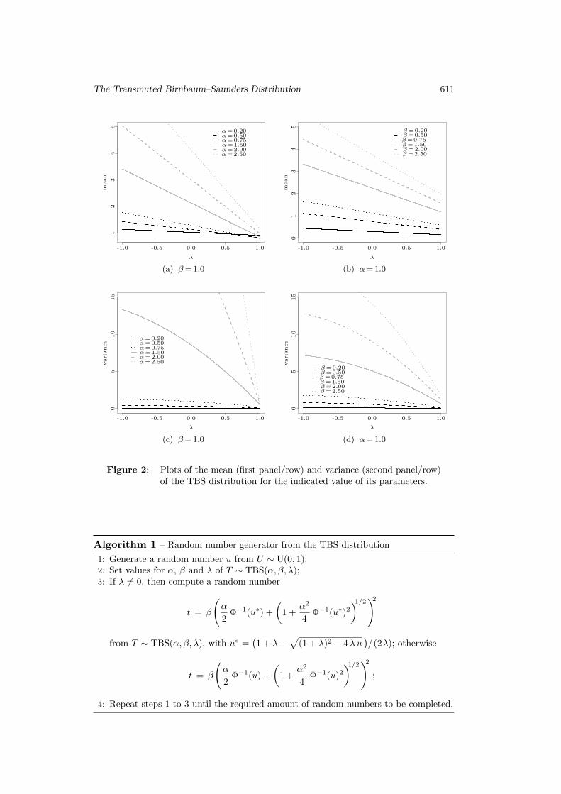
Figure 2 presents graphical plots of the mean (first panel/row) and variance

(second panel/row) of the TBS distribution for different values of α, β and λ.

Note that the mean and variance decrease as λ increases, but the mean and

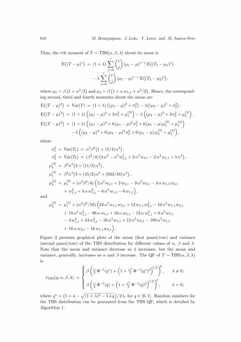
variance, generally, increases as α and β increase. The QF of T ∼ TBS(α, β, λ)

is

tTBS(q; α, β, λ) =

β

(α2 Φ−1(q∗) +

(1 + α2

4 Φ−1(q∗)2)1/2

)2, λ 6= 0;

β

(α2 Φ−1(q) +

(1 + α2

4 Φ−1(q)2)1/2

)2, λ = 0;

where q∗ =(1 + λ −

√(1 + λ)2 − 4 λ q

)/2λ, for q ∈ [0, 1]. Random numbers for

the TBS distribution can be generated from the TBS QF, which is detailed by

Algorithm 1.


mean

λ

α =0.20α =0.50α =0.75α =1.50α =2.00α =2.50

12

34

5

0.0 0.5 1.0-1.0 -0.5

(a) β = 1.0

mean

λ

β =0.20β =0.50β =0.75β =1.50β =2.00β =2.50

01

23

45

0.0 0.5 1.0-1.0 -0.5

(b) α = 1.0

vari

ance

λ

α =0.20α =0.50α =0.75α =1.50α =2.00α =2.50

05

0.0 0.5 1.0-1.0 -0.5

10

15

(c) β = 1.0

vari

ance

λ

β =0.20β =0.50β =0.75β =1.50β =2.00β =2.50

05

0.0 0.5 1.0-1.0 -0.5

10

15

(d) α = 1.0

Figure 2: Plots of the mean (first panel/row) and variance (second panel/row)of the TBS distribution for the indicated value of its parameters.

Algorithm 1 – Random number generator from the TBS distribution

1: Generate a random number u from U ∼ U(0, 1);2: Set values for α, β and λ of T ∼ TBS(α, β, λ);3: If λ 6= 0, then compute a random number

t = β

(α

2Φ−1(u∗) +

(1 +

α2

4Φ−1(u∗)2

)1/2)2

from T ∼ TBS(α, β, λ), with u∗ =(1 + λ −

√(1 + λ)2 − 4λu

)/(2λ); otherwise

t = β

(α

2Φ−1(u) +

(1 +

α2

4Φ−1(u)2

)1/2)2

;

4: Repeat steps 1 to 3 until the required amount of random numbers to be completed.


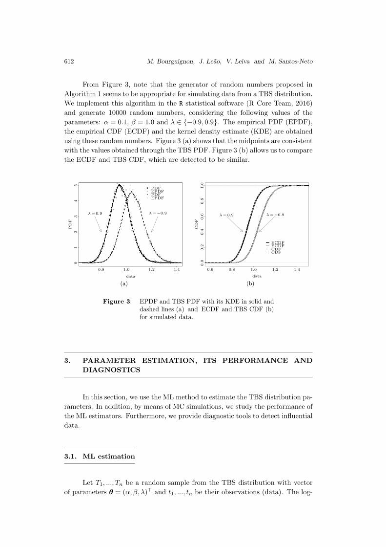
From Figure 3, note that the generator of random numbers proposed in

Algorithm 1 seems to be appropriate for simulating data from a TBS distribution.

We implement this algorithm in the R statistical software (R Core Team, 2016)

and generate 10000 random numbers, considering the following values of the

parameters: α = 0.1, β = 1.0 and λ ∈ −0.9, 0.9. The empirical PDF (EPDF),

the empirical CDF (ECDF) and the kernel density estimate (KDE) are obtained

using these random numbers. Figure 3 (a) shows that the midpoints are consistent

with the values obtained through the TBS PDF. Figure 3 (b) allows us to compare

the ECDF and TBS CDF, which are detected to be similar.

data

PD

F

PDFEPDFPDFEPDF

λ =0.9 λ =−0.9

01

23

45

0.8 1.0 1.2 1.4

(a)

data

CD

F

ECDFECDFCDFCDF

λ =0.9 λ =−0.9

0.0

0.2

0.4

0.6

0.6

0.8

0.8

1.0

1.0 1.2 1.4

(b)

Figure 3: EPDF and TBS PDF with its KDE in solid anddashed lines (a) and ECDF and TBS CDF (b)for simulated data.

3. PARAMETER ESTIMATION, ITS PERFORMANCE AND

DIAGNOSTICS

In this section, we use the ML method to estimate the TBS distribution pa-

rameters. In addition, by means of MC simulations, we study the performance of

the ML estimators. Furthermore, we provide diagnostic tools to detect influential

data.

3.1. ML estimation

Let T1, ..., Tn be a random sample from the TBS distribution with vector

of parameters θ = (α, β, λ)⊤ and t1, ..., tn be their observations (data). The log-


likelihood function for θ is

ℓ(θ) = n log(κ(α, β)

)− 3

2

n∑

i=1

log(ti) +n∑

i=1

log(ti + β)(3.1)

− 1

2α2

n∑

i=1

τ(ti/β) +n∑

i=1

log(1 + λ

(1 − 2Φ(vi)

)),

where vi = (1/α) ρ(ti/β). The ML estimate θ = (α, β, λ)⊤ is obtained by solving

the likelihood equations Uα = Uβ = Uλ = 0 simultaneously, where Uα, Uβ and Uλ

are the components of the score vector U(θ) = (Uα, Uβ, Uλ)⊤ given by

Uα = − n

α

(1 +

2

α2

)+

1

α3

n∑

i=1

(tiβ

+β

ti

)+

2λ

α

n∑

i=1

vi φ(vi)

1 + λ − 2λ Φ(vi),

Uβ = − n

2β+

n∑

i=1

1

ti + β+

1

2α2β

n∑

i=1

(tiβ

+β

ti

)− 2λ

αβ

n∑

i=1

(τ(√

ti/β)φ(vi)

1+λ−2λ Φ(vi)

),

Uλ =n∑

i=1

1 − 2 Φ(vi)

1 + λ(1 − 2 Φ(vi)

) ,

with φ being the standard normal PDF. The equations Uα = Uβ = Uλ = 0 cannot

be solved analytically, so that iterative techniques, such as bisection, Newton–

Raphson and secant methods, may be used; see Lange (2001) and McNamee and

Pa (2013). To obtain the ML estimates of the model parameters, we employ the

subroutine MaxBFGS of the Ox software; see Doornik (2006). This subroutine uses

the analytical derivatives to maximize ℓ(θ); see Nocedal and Wright (1999) and

Press et al. (2007). As starting values for the numerical procedure, we suggest to

consider

α =(s/β + β/r − 2

)1/2, β = (sr)1/2 , λ = 0,

where s = (1/n)∑n

i=1 ti and r = 1/((1/n)

∑ni=1(1/ti)

); see Birnbaum and Saun-

ders (1969a) and Leiva (2016, pp. 40–42).

To construct approximate confidence intervals and hypothesis tests for the

parameters, we use the normal approximation of the distribution of the ML es-

timator of θ = (α, β, λ)⊤. Specifically, assume that regularity conditions are ful-

filled in the interior of the parameter space but not on the boundary; see Cox

and Hinkley (1974). Then, the asymptotic distribution of√

n(θ−θ) is N3(0,Σθ),

where Σθ is the asymptotic variance–covariance matrix of θ, which can be ap-

proximated from the observed information matrix K(θ) = −J(θ), where J(θ) is


the Hessian matrix J(θ) = ∂2ℓ(θ)/∂θ∂θ⊤, whose elements are

Jαα =n

α2+

6n

α4− 4λ

α2

n∑

i=1

vi φ(vi)

1 + λ − 2λ Φ(vi)

(v2i +

vi φ(vi)

1 + λ − 2λ Φ(vi)− 2

)

− 3

4

n∑

i=1

(tiβ

+β

ti

),

Jαβ =2λ

α2β

n∑

i=1

τ(√

ti/β)φ(vi)

1 + λ(1 − 2Φ(vi)

)(

2λ vi φ(vi)

1 + λ(1 − 2Φ(vi)

) + (vi)2 − 1

)

− 1

α3β

n∑

i=1

(tiβ− β

xi

),

Jαλ = − 2

α

n∑

i=1

(vi φ(vi)(

1 + λ − 2λ Φ(vi))2

),

Jβλ =2

αβ

n∑

i=1

(τ(√

ti/β)φ(vi)(

1 + λ − 2λ Φ(vi))2

),

Jββ =λ

αβ2

n∑

i=1

φ(vi)

1 + λ − 2λ Φ(vi)

×(

3

√tiβ−√

β

ti−(τ(ti/β)

)2

α

(vi −

2λ φ(vi)

1 + λ − 2λ Φ(vi)

))

+n

2β2−

n∑

i=1

1

(ti + β)2− 1

α2β3

n∑

i=1

ti ,

Jλλ = −n∑

i=1

(1 − 2Φ(vi)

1 + λ(1 − 2Φ(vi)

))2

.

Thus, this trivariate normal distribution can be used to construct approximate

confidence intervals and regions for the model parameters. Note that asymptotic

100(1 − γ/2)% confidence intervals for α, β and λ are, respectively, established

as

α ± z1−γ/2

(Var(α)

)1/2, β ± z1−γ/2

(Var(β)

)1/2, λ ± z1−γ/2

(Var(λ)

)1/2,

where Var(θj) is the jth diagonal element of K−1(θ) related to each parameter

θj , for j = 1, 2, 3, with θ1 = α, θ2 = β, θ3 = λ, and zγ/2 is the 100(1 − γ/2)th

quantile of the standard normal distribution. Note that the estimated asymptotic

standard errors (SEs) of the each estimator can be obtained from the square root

of the diagonal element of K−1(θ).


3.2. Simulation study

We present a numerical experiment to evaluate the performance of the ML

estimators α, β and λ. The simulation was performed using the Ox software.

A number of 10000 MC replications were considered, sample sizes n ∈ 25, 50,

75, 100, 200, 400, 800, the combination of the parameters (α, β) ∈ (0.10, 1.00),

(0.50,1.00), (1.50,1.00), (2.00,1.00) and λ∈−0.80,−0.50,−0.20,0.20,0.50,0.80.Without loss of generality, we fix β at 1.00 in all experiments, because this is a

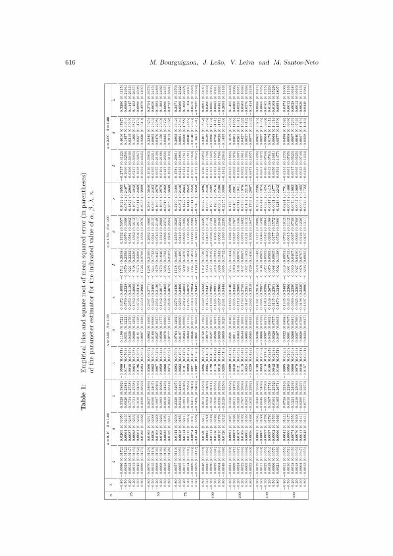
scale parameter. Table 1 presents the empirical bias and square root of mean

squared error of the estimators of the TBS distribution parameters. From this

table, note that, generally, the bias decreases as n increases, evidencing that the

ML estimators α and β are asymptotically unbiased. Observe that, when varying

the values of λ, the distributions of the estimators of α and β show, in general,

symmetrical behaviors. In addition, when the parameter α increases, the bias of β

increases. Note also that the estimator λ is more biased than α and β, considering

all scenarios. Also in all of the cases, the square root of the mean square error

decreases as n increases, proving that the ML estimators of the TBS distribution

parameters have good precision, as known. It is important to mention that some

iterations did not converge during the simulations, due possibly to the complexity

of the function to be maximized or because of the difficulty to provide a good

initial value from λ.

3.3. Influence diagnostics

Local influence is based on the curvature of the plane of the log-likelihood

function; see Leiva et al. (2014b, 2016b). In the case of the TBS model given in

(2.1), let θ = (α, β, λ)⊤ and ℓ(θ|ω) be the parameter vector and the log-likelihood

function related to this model perturbed by ω, respectively. The perturbation

vector ω belongs to a subset Ω ∈ Rn and ω0 is an n× 1 non-perturbation vector,

such that ℓ(θ|ω0) = ℓ(θ), for all θ. The corresponding likelihood distance (LD)

is

(3.2) LD(ω) = 2(ℓ(θ) − ℓ(θω)

),

where θω denotes the ML estimate of θ upon the perturbed TBS model used

to assess the influence of the perturbation on the ML estimate, whereas ℓ(θ)

is the usual likelihood function given in (3.1). Cook (1987) showed that the

normal curvature for θ in the direction of the vector d, with ‖d‖ = 1, is expressed

as Cd(θ) = 2 |d⊤∆⊤J(θ)−1∆d|, where ∆ is a 3×n perturbation matrix with

elements ∆ji = ∂2ℓ(θ|ω)/∂θj ∂ωi evaluated at θ = θ and ω = ω0, for j = 1, 2, 3,

i = 1, ..., n, and J(θ) is the corresponding Hessian matrix.


Table

1:

Em

pir

ical

bia

san

dsq

uar

ero

otof

mea

nsq

uar

eder

ror

(in

par

enth

eses

)of

the

par

amet

eres

tim

ator

for

the

indic

ated

valu

eof

α,β,λ,n.

nλ

α=

0.1

0,

β=

1.0

0α

=0.5

0,

β=

1.0

0α

=1.5

0,

β=

1.0

0α

=2.0

0,

β=

1.0

0

bα

b β

b λ

bα

b β

b λ

bα

b β

b λbαb βb λ

25

−0.8

0−

0.0

096

(0.0

172)

0.0

209

(0.0

305)

0.3

329

(0.3

892)

−0.0

509

(0.0

871)

0.1

198

(0.1

722)

0.3

472

(0.4

095)

−0.1

741

(0.2

818)

0.3

332

(0.5

057)

0.3

022

(0.3

853)

−0.2

717

(0.4

122)

0.4

616

(0.6

787)

0.3

296

(0.4

115)

−0.5

0−

0.0

038

(0.0

152)

0.0

064

(0.0

243)

0.0

926

(0.2

381)

−0.0

177

(0.0

763)

0.0

331

(0.1

222)

0.0

760

(0.2

328)

−0.0

670

(0.2

359)

0.0

970

(0.3

309)

0.0

502

(0.2

467)

−0.1

000

(0.3

250)

0.1

457

(0.4

034)

0.0

898

(0.2

494)

−0.2

0−

0.0

013

(0.0

147)

−0.0

087

(0.0

248)

−0.1

734

(0.2

738)

−0.0

048

(0.0

745)

−0.0

430

(0.1

179)

−0.2

053

(0.3

139)

−0.0

221

(0.2

232)

−0.0

581

(0.2

662)

−0.1

827

(0.2

988)

−0.0

306

(0.3

040)

−0.0

315

(0.3

069)

−0.1

447

(0.2

613)

0.2

0−

0.0

012

(0.0

145)

0.0

093

(0.0

253)

0.1

731

(0.2

738)

−0.0

064

(0.0

738)

0.0

500

(0.1

292)

0.1

952

(0.3

005)

−0.0

138

(0.2

236)

0.1

562

(0.3

613)

0.1

920

(0.3

042)

−0.0

247

(0.3

055)

0.1

369

(0.3

875)

0.1

453

(0.2

637)

0.5

0−

0.0

042

(0.0

152)

−0.0

061

(0.0

236)

−0.1

010

(0.2

436)

−0.0

196

(0.0

765)

−0.0

181

(0.1

128)

−0.0

736

(0.2

416)

−0.0

673

(0.2

380)

−0.0

104

(0.2

817)

−0.0

511

(0.2

469)

−0.1

038

(0.3

267)

−0.0

357

(0.3

175)

−0.0

896

(0.2

508)

0.8

0−

0.0

099

(0.0

175)

−0.0

198

(0.0

292)

−0.3

239

(0.3

822)

−0.0

484

(0.0

869)

−0.0

897

(0.1

338)

−0.3

350

(0.3

960)

−0.1

726

(0.2

788)

−0.1

858

(0.2

976)

−0.3

058

(0.3

889)

−0.2

662

(0.4

045)

−0.2

336

(0.3

510)

−0.3

278

(0.4

107)

50

−0.8

0−

0.0

070

(0.0

129)

0.0

165

(0.0

251)

0.2

627

(0.3

466)

−0.0

386

(0.0

667)

0.0

962

(0.1

406)

0.2

907

(0.3

771)

−0.1

295

(0.2

199)

0.2

662

(0.4

066)

0.2

680

(0.3

640)

−0.1

916

(0.3

083)

0.3

345

(0.5

025)

0.2

754

(0.3

675)

−0.5

0−

0.0

015

(0.0

110)

0.0

030

(0.0

200)

0.0

506

(0.2

407)

−0.0

062

(0.0

560)

0.0

160

(0.0

988)

0.0

420

(0.2

400)

−0.0

244

(0.1

733)

0.0

541

(0.2

515)

0.0

360

(0.2

483)

−0.0

395

(0.2

321)

0.0

862

(0.2

943)

0.0

650

(0.2

415)

−0.2

00.0

008

(0.0

106)

−0.0

108

(0.0

220)

−0.1

897

(0.2

940)

0.0

067

(0.0

549)

−0.0

527

(0.1

037)

−0.2

051

(0.3

136)

0.0

179

(0.1

645)

−0.0

743

(0.2

149)

−0.1

669

(0.2

879)

0.0

055

(0.2

139)

−0.0

476

(0.2

298)

−0.1

282

(0.2

489)

0.2

00.0

008

(0.0

106)

0.0

108

(0.0

223)

0.1

893

(0.2

928)

0.0

059

(0.0

544)

0.0

596

(0.1

177)

0.1

942

(0.3

017)

0.0

173

(0.1

646)

0.1

312

(0.2

860)

0.1

668

(0.2

870)

0.0

104

(0.2

168)

0.1

156

(0.2

930)

0.1

283

(0.2

492)

0.5

0−

0.0

018

(0.0

108)

−0.0

033

(0.0

195)

−0.0

618

(0.2

423)

−0.0

066

(0.0

550)

−0.0

070

(0.0

960)

−0.0

432

(0.2

405)

−0.0

203

(0.1

732)

0.0

066

(0.2

374)

−0.0

315

(0.2

462)

−0.0

427

(0.2

356)

−0.0

235

(0.2

572)

−0.0

696

(0.2

437)

0.8

0−

0.0

068

(0.0

128)

−0.0

159

(0.0

244)

−0.2

663

(0.3

514)

−0.0

374

(0.0

652)

−0.0

777

(0.1

149)

−0.2

848

(0.3

678)

−0.1

275

(0.2

167)

−0.1

605

(0.2

584)

−0.2

659

(0.3

639)

−0.1

932

(0.3

104)

−0.1

912

(0.2

992)

−0.2

727

(0.3

694)

75

−0.8

0−

0.0

057

(0.0

110)

0.0

144

(0.0

230)

0.2

320

(0.3

297)

−0.0

293

(0.0

560)

0.0

764

(0.1

202)

0.2

270

(0.3

430)

−0.1

118

(0.1

889)

0.2

359

(0.3

620)

0.2

490

(0.3

488)

−0.1

584

(0.2

681)

0.2

803

(0.4

342)

0.2

371

(0.3

370)

−0.5

0−

0.0

005

(0.0

095)

0.0

018

(0.0

185)

0.0

342

(0.2

449)

−0.0

023

(0.0

469)

0.0

107

(0.0

909)

0.0

250

(0.2

409)

−0.0

075

(0.1

480)

0.0

419

(0.2

244)

0.0

307

(0.2

446)

−0.0

213

(0.1

989)

0.0

661

(0.2

504)

0.0

566

(0.2

322)

−0.2

00.0

017

(0.0

093)

−0.0

114

(0.0

211)

−0.1

991

(0.3

046)

0.0

101

(0.0

473)

−0.0

504

(0.0

999)

−0.2

012

(0.3

082)

0.0

200

(0.1

370)

−0.0

656

(0.1

905)

−0.1

422

(0.2

664)

0.0

134

(0.1

761)

−0.0

500

(0.1

988)

−0.1

083

(0.2

278)

0.2

00.0

014

(0.0

091)

0.0

112

(0.0

213)

0.1

909

(0.2

965)

0.0

089

(0.0

467)

0.0

603

(0.1

115)

0.1

785

(0.3

028)

0.0

221

(0.1

384)

0.1

120

(0.2

508)

0.1

414

(0.2

652)

0.0

164

(0.1

781)

0.0

940

(0.2

485)

0.1

104

(0.2

307)

0.5

0−

0.0

009

(0.0

093)

−0.0

024

(0.0

181)

−0.0

471

(0.2

400)

−0.0

027

(0.0

469)

−0.0

046

(0.0

872)

−0.0

318

(0.2

384)

−0.0

084

(0.1

491)

0.0

038

(0.2

200)

−0.0

311

(0.2

458)

−0.0

207

(0.1

960)

−0.0

140

(0.2

333)

−0.0

570

(0.2

332)

0.8

0−

0.0

059

(0.0

112)

−0.0

144

(0.0

226)

−0.2

426

(0.3

408)

−0.0

307

(0.0

570)

−0.0

681

(0.1

063)

−0.2

469

(0.3

442)

−0.1

069

(0.1

887)

−0.1

469

(0.2

402)

−0.2

408

(0.3

450)

−0.1

571

(0.2

657)

−0.1

661

(0.2

691)

−0.2

337

(0.3

359)

100

−0.8

0−

0.0

048

(0.0

099)

0.0

130

(0.0

217)

0.2

072

(0.3

183)

−0.0

286

(0.0

528)

0.0

758

(0.1

195)

0.2

349

(0.3

233)

−0.1

012

(0.1

730)

0.2

152

(0.3

348)

0.2

272

(0.3

296)

−0.1

346

(0.2

385)

0.2

401

(0.3

852)

0.2

091

(0.3

107)

−0.5

00.0

000

(0.0

084)

0.0

008

(0.0

180)

0.0

204

(0.2

489)

0.0

005

(0.0

430)

0.0

072

(0.0

869)

0.0

176

(0.2

447)

−0.0

053

(0.1

353)

0.0

418

(0.2

114)

0.0

369

(0.2

440)

−0.0

147

(0.1

790)

0.0

539

(0.2

296)

0.0

490

(0.2

259)

−0.2

00.0

020

(0.0

082)

−0.0

111

(0.0

203)

−0.1

950

(0.3

011)

0.0

120

(0.0

430)

−0.0

527

(0.0

967)

−0.1

909

(0.2

905)

0.0

217

(0.1

219)

−0.0

596

(0.1

740)

−0.1

236

(0.2

492)

0.0

157

(0.1

562)

−0.0

396

(0.1

763)

−0.0

885

(0.2

105)

0.2

00.0

022

(0.0

081)

0.0

116

(0.0

208)

0.1

910

(0.2

955)

0.0

116

(0.0

424)

0.0

598

(0.1

087)

0.1

895

(0.2

931)

0.0

218

(0.1

231)

0.1

005

(0.2

302)

0.1

266

(0.2

516)

0.0

131

(0.1

557)

0.0

750

(0.2

141)

0.0

883

(0.2

091)

0.5

0−

0.0

004

(0.0

084)

−0.0

015

(0.0

176)

−0.0

330

(0.2

399)

−0.0

010

(0.0

418)

−0.0

020

(0.0

853)

−0.0

257

(0.2

366)

−0.0

026

(0.1

342)

0.0

052

(0.2

048)

−0.0

308

(0.2

406)

−0.0

140

(0.1

788)

−0.0

028

(0.2

171)

−0.0

481

(0.2

262)

0.8

0−

0.0

049

(0.0

098)

−0.0

126

(0.0

212)

−0.2

129

(0.3

250)

−0.0

285

(0.0

510)

−0.0

659

(0.1

025)

−0.2

401

(0.3

448)

−0.0

965

(0.1

712)

−0.1

363

(0.2

235)

−0.2

255

(0.3

300)

−0.1

342

(0.2

384)

−0.1

455

(0.2

500)

−0.2

093

(0.3

116)

200

−0.8

0−

0.0

031

(0.0

079)

0.0

091

(0.0

187)

0.1

530

(0.2

852)

−0.0

209

(0.0

434)

0.0

591

(0.1

046)

0.1

863

(0.3

146)

−0.0

744

(0.1

414)

0.1

624

(0.2

709)

0.1

780

(0.2

829)

−0.0

935

(0.1

885)

0.1

619

(0.2

863)

0.1

455

(0.2

440)

−0.5

00.0

009

(0.0

071)

−0.0

007

(0.0

168)

−0.0

011

(0.2

470)

0.0

040

(0.0

357)

0.0

011

(0.0

810)

0.0

035

(0.2

458)

0.0

070

(0.1

115)

0.0

187

(0.1

767)

0.0

160

(0.2

201)

−0.0

003

(0.1

376)

0.0

301

(0.1

785)

0.0

300

(0.1

906)

−0.2

00.0

024

(0.0

067)

−0.0

107

(0.0

192)

−0.1

820

(0.2

963)

0.0

121

(0.0

352)

−0.0

463

(0.0

884)

−0.1

712

(0.2

969)

0.0

138

(0.0

870)

−0.0

353

(0.1

346)

−0.0

717

(0.1

941)

0.0

106

(0.1

097)

−0.0

261

(0.1

331)

−0.0

525

(0.1

657)

0.2

00.0

022

(0.0

066)

0.0

108

(0.0

193)

0.1

767

(0.2

896)

0.0

119

(0.0

344)

0.0

544

(0.1

005)

0.1

704

(0.2

758)

0.0

157

(0.0

887)

0.0

578

(0.1

692)

0.0

739

(0.1

976)

0.0

092

(0.1

081)

0.0

427

(0.1

522)

0.0

503

(0.1

638)

0.5

00.0

003

(0.0

068)

−0.0

005

(0.0

165)

−0.0

202

(0.2

386)

0.0

024

(0.0

345)

0.0

005

(0.0

802)

−0.0

187

(0.2

351)

0.0

057

(0.1

102)

0.0

121

(0.1

813)

−0.0

167

(0.2

213)

−0.0

002

(0.1

395)

0.0

027

(0.1

812)

−0.0

276

(0.1

928)

0.8

0−

0.0

033

(0.0

080)

−0.0

096

(0.0

189)

−0.1

635

(0.2

992)

−0.0

229

(0.0

424)

−0.0

565

(0.0

943)

−0.2

092

(0.3

319)

−0.0

729

(0.1

410)

−0.1

092

(0.1

947)

−0.1

794

(0.2

867)

−0.0

871

(0.1

857)

−0.0

977

(0.2

032)

−0.1

414

(0.2

419)

400

−0.8

0−

0.0

019

(0.0

066)

0.0

061

(0.0

164)

0.1

043

(0.2

538)

−0.0

139

(0.0

369)

0.0

436

(0.0

923)

0.1

391

(0.2

816)

−0.0

518

(0.1

143)

0.1

117

(0.2

098)

0.1

254

(0.2

238)

−0.0

547

(0.1

498)

0.0

962

(0.2

075)

0.0

886

(0.1

817)

−0.5

00.0

011

(0.0

060)

−0.0

009

(0.0

160)

−0.0

048

(0.2

436)

0.0

053

(0.0

308)

−0.0

006

(0.0

759)

0.0

005

(0.2

387)

0.0

106

(0.0

902)

0.0

048

(0.1

430)

0.0

047

(0.1

874)

0.0

061

(0.1

072)

0.0

097

(0.1

365)

0.0

068

(0.1

525)

−0.2

00.0

022

(0.0

055)

−0.0

097

(0.0

176)

−0.1

595

(0.2

790)

0.0

116

(0.2

770)

−0.0

387

(0.0

813)

−0.1

410

(0.0

298)

0.0

072

(0.0

592)

−0.0

142

(0.0

994)

−0.0

323

(0.1

424)

0.0

040

(0.0

760)

−0.0

064

(0.0

980)

−0.0

165

(0.1

215)

0.2

00.0

019

(0.0

054)

0.0

097

(0.0

178)

0.1

567

(0.2

751)

0.0

109

(0.0

287)

0.0

439

(0.0

902)

0.1

348

(0.2

673)

0.0

070

(0.0

593)

0.0

269

(0.1

108)

0.0

317

(0.1

415)

0.0

043

(0.0

764)

0.0

178

(0.1

041)

0.0

188

(0.1

220)

0.5

00.0

006

(0.0

057)

−0.0

002

(0.0

153)

−0.0

164

(0.2

352)

0.0

042

(0.0

298)

0.0

028

(0.0

757)

−0.0

135

(0.2

301)

0.0

098

(0.0

905)

0.0

177

(0.1

572)

−0.0

041

(0.1

877)

0.0

056

(0.1

061)

0.0

068

(0.1

431)

−0.0

108

(0.1

529)

0.8

0−

0.0

021

(0.0

066)

−0.0

066

(0.0

166)

−0.1

165

(0.2

671)

−0.0

186

(0.0

371)

−0.0

497

(0.0

903)

−0.1

870

(0.3

240)

−0.0

502

(0.1

138)

−0.0

739

(0.1

588)

−0.1

213

(0.2

242)

−0.0

503

(0.1

477)

−0.0

577

(0.1

659)

−0.0

854

(0.1

807)

800

−0.8

0−

0.0

011

(0.0

055)

0.0

041

(0.0

141)

0.0

728

(0.2

216)

−0.0

095

(0.0

320)

0.0

322

(0.0

808)

0.1

045

(0.2

482)

−0.0

348

(0.0

951)

0.0

733

(0.1

612)

0.0

821

(0.1

731)

−0.0

244

(0.1

233)

0.0

498

(0.1

568)

0.0

474

(0.1

400)

−0.5

00.0

010

(0.0

051)

−0.0

006

(0.0

147)

0.0

010

(0.2

286)

0.0

050

(0.0

266)

−0.0

001

(0.0

707)

0.0

043

(0.2

266)

0.0

091

(0.0

713)

−0.0

015

(0.1

112)

−0.0

037

(0.1

466)

0.0

061

(0.0

765)

0.0

008

(0.0

969)

−0.0

012

(0.1

116)

−0.2

00.0

018

(0.0

045)

−0.0

074

(0.0

155)

−0.1

224

(0.2

494)

0.0

086

(0.0

239)

−0.0

266

(0.0

681)

−0.0

960

(0.2

350)

0.0

030

(0.0

407)

−0.0

037

(0.0

730)

−0.0

079

(0.1

063)

0.0

017

(0.0

523)

0.0

007

(0.0

723)

−0.0

028

(0.0

918)

0.2

00.0

018

(0.0

045)

0.0

076

(0.0

160)

0.1

218

(0.2

506)

0.0

079

(0.0

233)

0.0

307

(0.0

769)

0.0

925

(0.2

305)

0.0

027

(0.0

410)

0.0

093

(0.0

760)

0.0

097

(0.1

069)

0.0

005

(0.0

525)

0.0

040

(0.0

736)

0.0

012

(0.0

910)

0.5

00.0

004

(0.0

047)

−0.0

011

(0.0

141)

−0.0

290

(0.2

227)

0.0

040

(0.0

261)

0.0

028

(0.0

708)

−0.0

108

(0.2

230)

0.0

078

(0.0

707)

0.0

124

(0.1

238)

−0.0

005

(0.1

465)

0.0

033

(0.0

749)

0.0

057

(0.1

015)

−0.0

036

(0.1

113)

0.8

0−

0.0

013

(0.0

055)

−0.0

043

(0.0

141)

−0.0

777

(0.2

273)

−0.0

157

(0.0

331)

−0.0

424

(0.0

827)

−0.1

607

(0.2

990)

−0.0

293

(0.0

925)

−0.0

437

(0.1

311)

−0.0

743

(0.1

723)

−0.0

229

(0.1

234)

−0.0

258

(0.1

416)

−0.0

449

(0.1

384)


A local influence diagnostic is generally based on index plots. For example,

the index graph of the eigenvector dmax related to the maximum eigenvalue of

B(θ) = −∆⊤J(θ)−1∆, Cdmax(θ) say, evaluated at θ = θ, can detect those cases

that, under small perturbations, exercise a high influence on LD(ω) given in

(3.2). In addition to the direction vector of maximum normal curvature, dmax

say, another direction of interest is di = ein, which corresponds to the direction of

the case i, where ein is an n×1 vector of zeros with a value equal to one at the ith

position, that is, ein, 1 ≤ i ≤ n is the canonical basis of Rn. Thus, the normal

curvature is Ci(θ) = 2|bii|, where bii is the ith diagonal element of B(θ), for

i = 1, ..., n, evaluated at θ = θ. The case i is considered as potentially influential

if Ci(θ) > 2C(θ), where C(θ) =∑n

i=1 Ci(θ)/n. This procedure is called total

local influence of the case i; see Liu et al. (2016).

Consider the log-likelihood function given in (3.1). We obtain the respec-

tive perturbation matrix ∆, which is already evaluated at the non-perturbation

vector ω0, under the scheme of case-weight perturbation. Then, we want to eval-

uate whether cases with different weights in the log-likelihood function affect the

ML estimate of θ. This scheme is the most used to assess local influence in a

model. The log-likelihood function of the TBS model perturbed by the case-

weight scheme is

ℓ(θ|ω) =n∑

i=1

ℓi(θ|ωi) =n∑

i=1

ωi ℓi(θ) .

Then, taking its derivative with respect to ω⊤, we obtain ∆ = (∆β ,∆α,∆λ)⊤.

After evaluating at θ = θ and ω = ω0, the elements of ∆α, ∆β and ∆λ are

∆(i)α = − 1

α

(1 +

2

α2

)+

1

α3

(tiβ

+β

ti

)+

2λ vi φ(vi)

α(1 + λ − 2λ Φ(vi)

) , i = 1, ..., n ,

∆(i)λ =

1 − 2Φ(vi)

1 + λ(1 − 2Φ(vi)

) ,

∆(i)β = − 1

2β+

1

ti + β+

1

2α2β

(tiβ

+β

ti

)− 2λ

αβ

(τ(√

ti/β)φ(vi)

1 + λ − 2λ Φ(vi)

).

4. APPLICATIONS TO REAL-WORLD DATA

In this section, we apply the obtained results for the new model to three

data sets, illustrating its potential applications. The results are compared to

other competing BS distributions. All the computations were done using the

Ox software. For each data set, we estimate the unknown parameters of the

associated distribution by the ML method and evaluate its goodness of fit with

suitable methods.


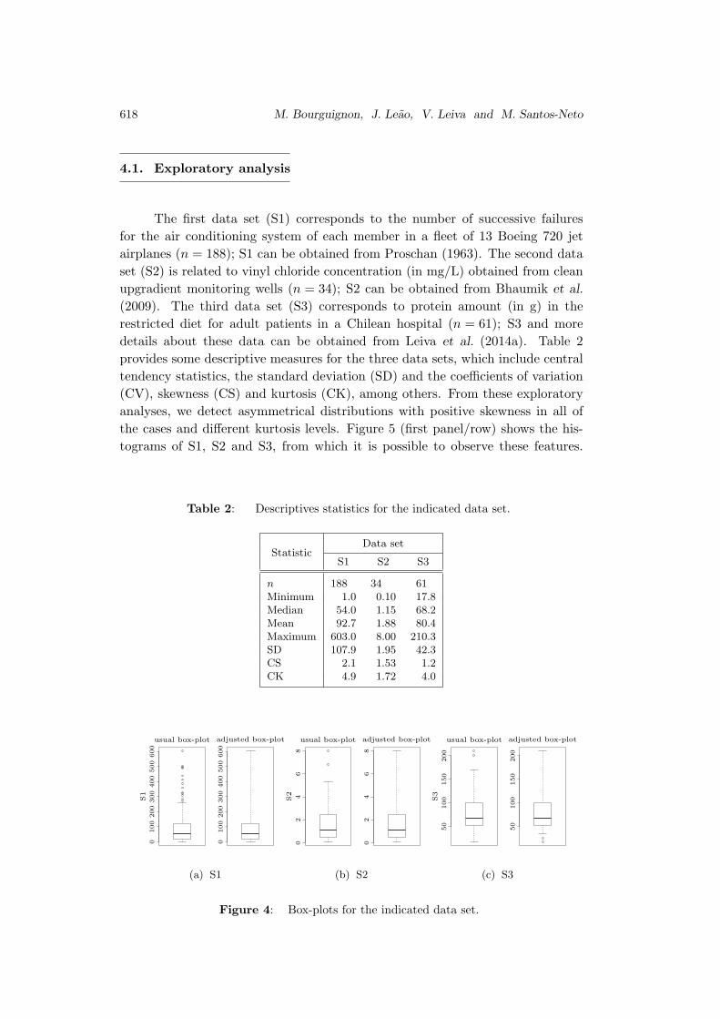
4.1. Exploratory analysis

The first data set (S1) corresponds to the number of successive failures

for the air conditioning system of each member in a fleet of 13 Boeing 720 jet

airplanes (n = 188); S1 can be obtained from Proschan (1963). The second data

set (S2) is related to vinyl chloride concentration (in mg/L) obtained from clean

upgradient monitoring wells (n = 34); S2 can be obtained from Bhaumik et al.

(2009). The third data set (S3) corresponds to protein amount (in g) in the

restricted diet for adult patients in a Chilean hospital (n = 61); S3 and more

details about these data can be obtained from Leiva et al. (2014a). Table 2

provides some descriptive measures for the three data sets, which include central

tendency statistics, the standard deviation (SD) and the coefficients of variation

(CV), skewness (CS) and kurtosis (CK), among others. From these exploratory

analyses, we detect asymmetrical distributions with positive skewness in all of

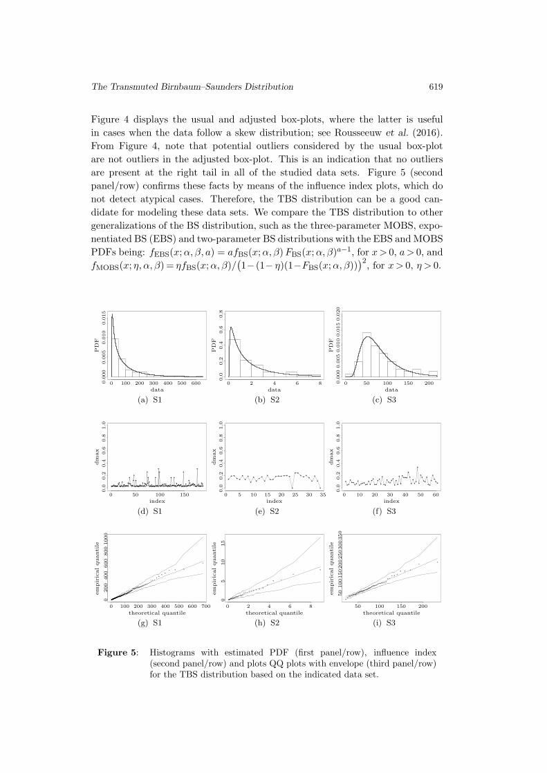
the cases and different kurtosis levels. Figure 5 (first panel/row) shows the his-

tograms of S1, S2 and S3, from which it is possible to observe these features.

Table 2: Descriptives statistics for the indicated data set.

StatisticData set

S1 S2 S3

n 188 34 61Minimum 1.0 0.10 17.8Median 54.0 1.15 68.2Mean 92.7 1.88 80.4Maximum 603.0 8.00 210.3SD 107.9 1.95 42.3CS 2.1 1.53 1.2CK 4.9 1.72 4.0

00

100

100

200

200

300

300

400

400

500

500

600

600

S1

usual box-plot adjusted box-plot

(a) S1

22

44

66

88

00

S2


(b) S2

50

50

100

100

150

150

200

200

S3


(c) S3

Figure 4: Box-plots for the indicated data set.


Figure 4 displays the usual and adjusted box-plots, where the latter is useful

in cases when the data follow a skew distribution; see Rousseeuw et al. (2016).

From Figure 4, note that potential outliers considered by the usual box-plot

are not outliers in the adjusted box-plot. This is an indication that no outliers

are present at the right tail in all of the studied data sets. Figure 5 (second

panel/row) confirms these facts by means of the influence index plots, which do

not detect atypical cases. Therefore, the TBS distribution can be a good can-

didate for modeling these data sets. We compare the TBS distribution to other

generalizations of the BS distribution, such as the three-parameter MOBS, expo-

nentiated BS (EBS) and two-parameter BS distributions with the EBS and MOBS

PDFs being: fEBS(x; α, β, a) = afBS(x; α, β)FBS(x; α, β)a−1, for x > 0, a > 0, and

fMOBS(x; η, α, β) = ηfBS(x; α, β)/(1− (1− η)(1−FBS(x; α, β))

)2, for x > 0, η > 0.

data

PD

F

0.0

00

0.0

15

0.0

05

0.0

10

300200 400 500 6000 100

(a) S1

data

PD

F

80 2 4 6

0.0

0.2

0.4

0.6

0.8

(b) S2

data

PD

F

0.0

00

0.0

20

0.0

15

0.0

05

0.0

10

2000 50 100 150

(c) S3

0

dm

ax

index

0.0

0.2

0.4

0.6

0.8

1.0

50 100 150

(d) S1

0 5

dm

ax

index

0.0

0.2

0.4

0.6

0.8

1.0

10 15 20 25 30 35

(e) S2

0

dm

ax

index

0.0

0.2

0.4

0.6

0.8

1.0

10 20 30 5040 60

(f) S3

theoretical quantile

em

pir

icalquanti

le

300

200

200

400

400 500

600

600

800

700

1000

0

0 100

(g) S1


em

pir

icalquanti

le

8

0

0 2 4 6

510

15

(h) S2


em

pir

icalquanti

le

300

200

200

250

350

50

50

100

100

150

150

(i) S3

Figure 5: Histograms with estimated PDF (first panel/row), influence index(second panel/row) and plots QQ plots with envelope (third panel/row)for the TBS distribution based on the indicated data set.


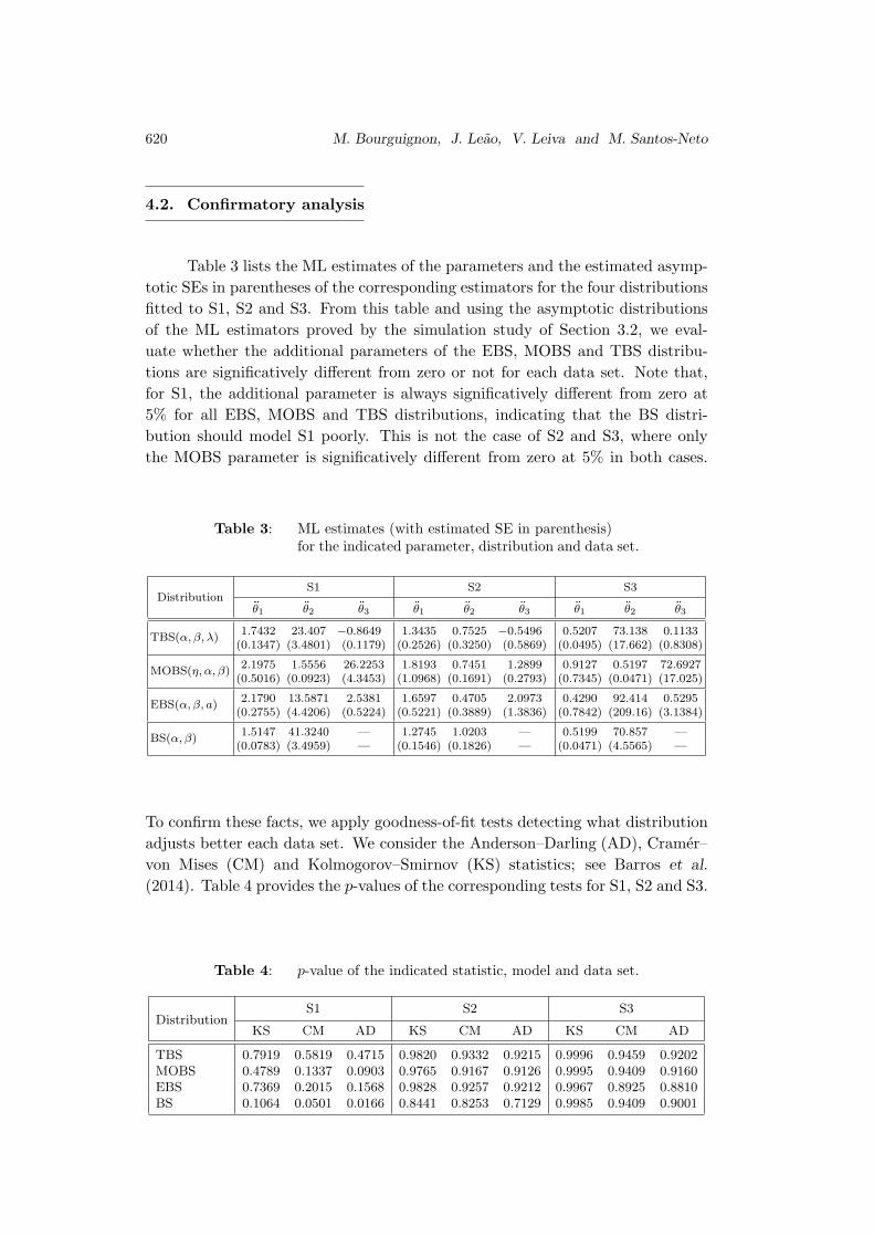
4.2. Confirmatory analysis

Table 3 lists the ML estimates of the parameters and the estimated asymp-

totic SEs in parentheses of the corresponding estimators for the four distributions

fitted to S1, S2 and S3. From this table and using the asymptotic distributions

of the ML estimators proved by the simulation study of Section 3.2, we eval-

uate whether the additional parameters of the EBS, MOBS and TBS distribu-

tions are significatively different from zero or not for each data set. Note that,

for S1, the additional parameter is always significatively different from zero at

5% for all EBS, MOBS and TBS distributions, indicating that the BS distri-

bution should model S1 poorly. This is not the case of S2 and S3, where only

the MOBS parameter is significatively different from zero at 5% in both cases.

Table 3: ML estimates (with estimated SE in parenthesis)for the indicated parameter, distribution and data set.

DistributionS1 S2 S3bθ1bθ2

bθ3bθ1

bθ2bθ3

bθ1bθ2

bθ3

TBS(α, β, λ)1.7432 23.407 −0.8649 1.3435 0.7525 −0.5496 0.5207 73.138 0.1133

(0.1347) (3.4801) (0.1179) (0.2526) (0.3250) (0.5869) (0.0495) (17.662) (0.8308)

MOBS(η, α, β)2.1975 1.5556 26.2253 1.8193 0.7451 1.2899 0.9127 0.5197 72.6927

(0.5016) (0.0923) (4.3453) (1.0968) (0.1691) (0.2793) (0.7345) (0.0471) (17.025)

EBS(α, β, a)2.1790 13.5871 2.5381 1.6597 0.4705 2.0973 0.4290 92.414 0.5295

(0.2755) (4.4206) (0.5224) (0.5221) (0.3889) (1.3836) (0.7842) (209.16) (3.1384)

BS(α, β)1.5147 41.3240 — 1.2745 1.0203 — 0.5199 70.857 —

(0.0783) (3.4959) — (0.1546) (0.1826) — (0.0471) (4.5565) —

To confirm these facts, we apply goodness-of-fit tests detecting what distribution

adjusts better each data set. We consider the Anderson–Darling (AD), Cramer–

von Mises (CM) and Kolmogorov–Smirnov (KS) statistics; see Barros et al.

(2014). Table 4 provides the p-values of the corresponding tests for S1, S2 and S3.

Table 4: p-value of the indicated statistic, model and data set.

DistributionS1 S2 S3

KS CM AD KS CM AD KS CM AD

TBS 0.7919 0.5819 0.4715 0.9820 0.9332 0.9215 0.9996 0.9459 0.9202MOBS 0.4789 0.1337 0.0903 0.9765 0.9167 0.9126 0.9995 0.9409 0.9160EBS 0.7369 0.2015 0.1568 0.9828 0.9257 0.9212 0.9967 0.8925 0.8810BS 0.1064 0.0501 0.0166 0.8441 0.8253 0.7129 0.9985 0.9409 0.9001


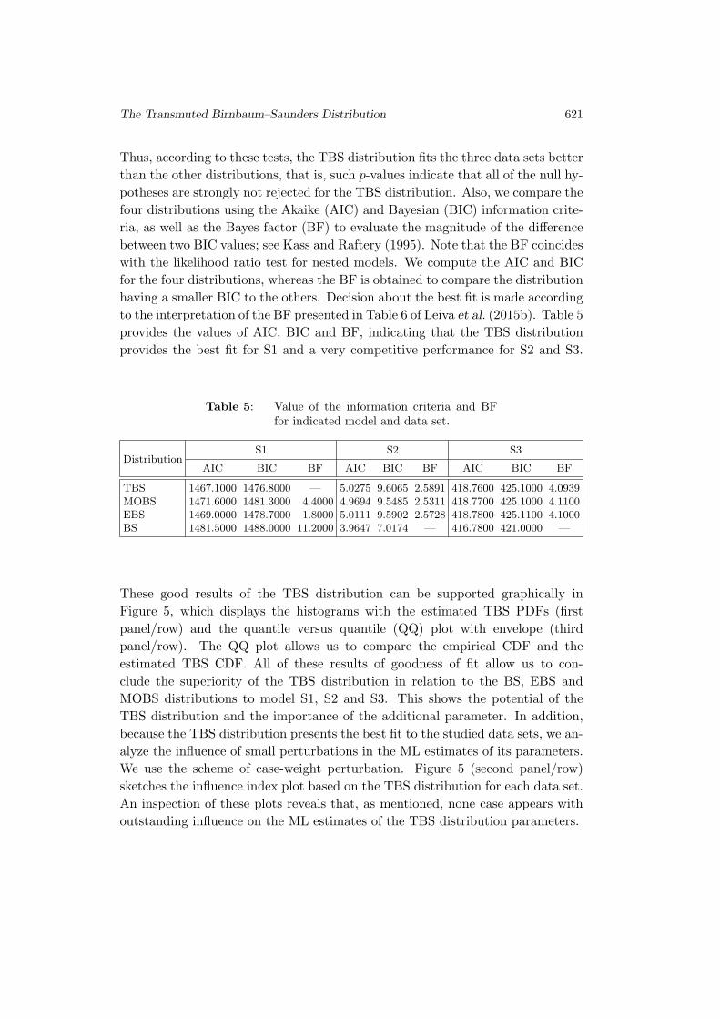
Thus, according to these tests, the TBS distribution fits the three data sets better

than the other distributions, that is, such p-values indicate that all of the null hy-

potheses are strongly not rejected for the TBS distribution. Also, we compare the

four distributions using the Akaike (AIC) and Bayesian (BIC) information crite-

ria, as well as the Bayes factor (BF) to evaluate the magnitude of the difference

between two BIC values; see Kass and Raftery (1995). Note that the BF coincides

with the likelihood ratio test for nested models. We compute the AIC and BIC

for the four distributions, whereas the BF is obtained to compare the distribution

having a smaller BIC to the others. Decision about the best fit is made according

to the interpretation of the BF presented in Table 6 of Leiva et al. (2015b). Table 5

provides the values of AIC, BIC and BF, indicating that the TBS distribution

provides the best fit for S1 and a very competitive performance for S2 and S3.

Table 5: Value of the information criteria and BFfor indicated model and data set.

DistributionS1 S2 S3

AIC BIC BF AIC BIC BF AIC BIC BF

TBS 1467.1000 1476.8000 — 5.0275 9.6065 2.5891 418.7600 425.1000 4.0939MOBS 1471.6000 1481.3000 4.4000 4.9694 9.5485 2.5311 418.7700 425.1000 4.1100EBS 1469.0000 1478.7000 1.8000 5.0111 9.5902 2.5728 418.7800 425.1100 4.1000BS 1481.5000 1488.0000 11.2000 3.9647 7.0174 — 416.7800 421.0000 —

These good results of the TBS distribution can be supported graphically in

Figure 5, which displays the histograms with the estimated TBS PDFs (first

panel/row) and the quantile versus quantile (QQ) plot with envelope (third

panel/row). The QQ plot allows us to compare the empirical CDF and the

estimated TBS CDF. All of these results of goodness of fit allow us to con-

clude the superiority of the TBS distribution in relation to the BS, EBS and

MOBS distributions to model S1, S2 and S3. This shows the potential of the

TBS distribution and the importance of the additional parameter. In addition,

because the TBS distribution presents the best fit to the studied data sets, we an-

alyze the influence of small perturbations in the ML estimates of its parameters.

We use the scheme of case-weight perturbation. Figure 5 (second panel/row)

sketches the influence index plot based on the TBS distribution for each data set.

An inspection of these plots reveals that, as mentioned, none case appears with

outstanding influence on the ML estimates of the TBS distribution parameters.


5. CONCLUSIONS AND FUTURE RESEARCH

We have used the transmutation method to define a new distribution that

generalizes the Birnbaum–Saunders model, named the transmuted Birnbaum–

Saunders distribution. Some relevant characteristics of the new distribution have

been derived, such as the probabilistic functions, as well moments and a gen-

erator of random numbers. We have estimated the model parameters with the

maximum likelihood method and its good performance has been evaluated by

means of Monte Carlo simulations. Score vector and Hessian matrix were de-

rived to infer about the model parameters. Diagnostic tools have been obtained

to detect locally influential data in the maximum likelihood estimates. Poten-

tial applications of the new distribution have been considered by using three

real-world data sets. Goodness-of-fit methods have demonstrated the suitable

performance of the transmuted Birnbaum–Saunders distribution to these data in

comparison to other versions of the Birnbaum–Saunders distribution. We hope

that the new proposed distribution may attract wider applications in statistics.

Modeling based on fixed, random and mixed effects, including semi-parametric

formulations and non-parametric estimation of kernel, can be conducted with this

new distribution. Multivariate versions, as well as copula methods, could also be

addressed by the new transmuted Birnbaum–Saunders distribution.

ACKNOWLEDGMENTS

The authors thank the editors and reviewers for their constructive com-

ments on an earlier version of this manuscript which resulted in this improved

version. This research was supported by Capes and CNPq from Brazil, and

FONDECYT 1160868 grant from Chile.


REFERENCES

[1] Ahmed, S.; Castro-Kuriss, C.; Leiva, V.; Flores, E. and Sanhueza,

A. (2010). Truncated version of the Birnbaum–Saunders distribution with anapplication in financial risk, Pakistan Journal of Statistics, 26, 293–311.

[2] Aryal, G. (2013). Transmuted log-logistic distribution, Journal of Statistics

Applications and Probability, 2, 11–20.

[3] Aryal, G. and Tsokos, C. (2009). On the transmuted extreme value distri-bution with application, Nonlinear Analysis: Theory, Methods and Applications,71, 1401–1407.

[4] Aryal, G. and Tsokos, C. (2011). Transmuted Weibull distribution: A gener-alization of the Weibull probability distribution, European Journal of Pure and

Applied Mathematics, 4, 89–102.

[5] Ashour, S. and Eltehiwy, M. (2013). Transmuted Lomax distribution, Amer-

ican Journal of Applied Mathematics and Statistics, 1, 121–127.

[6] Athayde, E.; Azevedo, C.; Leiva, V. and Sanhueza, A. (2012). AboutBirnbaum–Saunders distributions based on the Johnson system, Communications

in Statistics: Theory and Methods, 41, 2061–2079.

[7] Azevedo, C.; Leiva, V.; Athayde, E. and Balakrishnan, N. (2012). Shapeand change point analyses of the Birnbaum–Saunders-t hazard rate and associatedestimation, Computational Statistics and Data Analysis, 56, 3887–3897.

[8] Azzalini, A. (1985). A class of distributions which includes the normal ones,Scandinavian Journal of Statistics, 11, 171–178.

[9] Balakrishnan, N.; Gupta, R.; Kundu, D.; Leiva, V. and Sanhueza, A.

(2011). On some mixture models based on the Birnbaum–Saunders distribu-tion and associated inference, Journal of Statistical Planning and Inference, 141,2175–2190.

[10] Barros, M.; Leiva, V.; Ospina, R. and Tsuyuguchi, A. (2014). Goodness-of-fit tests for the Birnbaum–Saunders distribution with censored reliability data,IEEE Transactions on Reliability, 63, 543–554.

[11] Bhaumik, D.; Kapur, K. and Gibbons, R. (2009). Testing parameters of agamma distribution for small samples, Technometrics, 51, 326–334.

[12] Birnbaum, Z.W. and Saunders, S.C. (1969a). Estimation for a family oflife distributions with applications to fatigue, Journal of Applied Probability, 6,328–347.

[13] Birnbaum, Z.W. and Saunders, S.C. (1969b). A new family of life distribu-tions, Journal of Applied Probability, 6, 319–327.

[14] Bourguignon, M.; Silva, R. and Cordeiro, G. (2014). A new class of fa-tigue life distributions, Journal of Statistical Computation and Simulation, 84,2619–2635.

[15] Castillo, N.; Gomez, H. and Bolfarine, H. (2011). Epsilon Birnbaum–Saunders distribution family: Properties and inference, Statistical Papers, 52,871–883.


[16] Cook, R.D. (1987). Influence assessment, Journal of Applied Statistics, 14,117–131.

[17] Cordeiro, M. and Lemonte, J. (2011). The β-Birnbaum–Saunders distribu-tion: An improved distribution for fatigue life modeling, Computational Statistics

and Data Analysis, 55, 1445–1461.

[18] Cornish, E.A. and Fisher, R.A. (1937). Moments and cumulants in thespecification of distributions, Review of the International Statistical Institute, 5,307–320.

[19] Cox, D.R. and Hinkley, D.V. (1974). Theoretical Statistics, Chapman andHall, London, UK.

[20] Desousa, M.F.; Saulo, H.; Leiva, V. and Scalco, P. (2017).On a tobit-Birnbaum–Saunders model with an application to antibody re-sponse to vaccine, Journal of Applied Statistics, page in press available athttp://dx.doi.org/10.1080/02664763.2017.1322559.

[21] Dıaz-Garcıa, J. and Leiva, V. (2005). A new family of life distributions basedon elliptically contoured distributions, Journal of Statistical Planning and Infer-

ence, 128, 445–457.

[22] Doornik, J. (2006). An Object-Oriented Matrix Language, Timberlake Consul-tants Press, London, UK.

[23] Edgeworth, F.Y. (1917). On the mathematical representation of statisticaldata, Journal of the Royal Statistical Society A, 80, 65–83; 266–288; 411–437.

[24] Ferreira, M.; Gomes, M.I. and Leiva, V. (2012). On an extreme valueversion of the Birnbaum–Saunders distribution, REVSTAT Statistical Journal,10, 181–210.

[25] Fierro, R.; Leiva, V.; Ruggeri, F. and Sanhueza, A. (2013). On aBirnbaum–Saunders distribution arising from a non-homogeneous Poisson pro-cess, Statistical and Probability Letters, 83, 1233–1239.

[26] Garcia-Papani, F.; Uribe-Opazo, M.A.; Leiva, V. and Aykroyd, R.G.

(2017). Birnbaum–Saunders spatial modelling and diagnostics applied to agricul-tural engineering data, Stochastic Environmental Research and Risk Assessment,31, 105–124.

[27] Gomez, H.; Olivares-Pacheco, J.F. and Bolfarine, H. (2009). An exten-sion of the generalized Birnbaum–Saunders distribution, Statistical and Probabil-

ity Letters, 79, 331–338.

[28] Gradshteyn, I. and Randzhik, I. (2000). Table of Integrals, Series, and Prod-

ucts, Academic Press, New York, US.

[29] Guiraud, P.; Leiva, V. and Fierro, R. (2009). A non-central version of theBirnbaum–Saunders distribution for reliability analysis, IEEE Transactions on

Reliability, 58, 152–160.

[30] Johnson, N.; Kotz, S. and Balakrishnan, N. (1994). Continuous Univariate

Distributions, volume 1, Wiley, New York, US.

[31] Johnson, N.; Kotz, S. and Balakrishnan, N. (1995). Continuous Univariate

Distributions, volume 2, Wiley, New York, US.

[32] Johnson, N.L. (1949). Systems of frequency curves generated by methods oftranslation, Biometrika, 36, 149–176.


[33] Kass, R. and Raftery, A. (1995). Bayes factors, Journal of the American

Statistical Association, 90, 773–795.

[34] Khan, M. and King, R. (2013). Transmuted modified Weibull distribution:A generalization of the modified Weibull probability distribution, European Jour-

nal of Pure and Applied Mathematics, 6, 66–88.

[35] Khan, M. and King, R. (2014). A new class of transmuted inverse Weibulldistribution for reliability analysis, American Journal of Mathematical and Man-

agement, 33, 261–286.

[36] Kotz, S.; Leiva, V. and Sanhueza, A. (2010). Two new mixture models re-lated to the inverse Gaussian distribution, Methodology and Computing in Applied

Probability, 12, 199–212.

[37] Lange, K. (2001). Numerical Analysis for Statisticians, Springer, New York,US.

[38] Leao, J.; Leiva, V.; Saulo, H. and Tomazella, V. (2017a). A survivalmodel with Birnbaum–Saunders frailty for uncensored and censored cancer data,Brazilian Journal of Probability and Statistics, page in press.

[39] Leao, J.; Leiva, V.; Saulo, H. and Tomazella, V. (2017b). Birnbaum–Saunders frailty regression models: Diagnostics and application to medical data,Biometrical Journal, 59, 291–314.

[40] Leiva, V. (2016). The Birnbaum–Saunders Distribution, Academic Press, NewYork, US.

[41] Leiva, V.; Athayde, E.; Azevedo, C. and Marchant, C. (2011). Modelingwind energy flux by a Birnbaum–Saunders distribution with unknown shift pa-rameter, Journal of Applied Statistics, 38, 2819–2838.

[42] Leiva, V.; Ferreira, M.; Gomes, M.I. and Lillo, C. (2016a). Extreme valueBirnbaum–Saunders regression models applied to environmental data, Stochastic

Environmental Research and Risk Assessment, 30, 1045–1058.

[43] Leiva, V.; Liu, S.; Shi, L. and Cysneiros, F. (2016b). Diagnostics in ellipticalregression models with stochastic restrictions applied to econometrics, Journal of

Applied Statistics, 43, 627–642.

[44] Leiva, V.; Marchant, C.; Ruggeri, F. and Saulo, H. (2015a). A criterionfor environmental assessment using Birnbaum–Saunders attribute control charts,Environmetrics, 26, 463–476.

[45] Leiva, V.; Marchant, C.; Saulo, H.; Aslam, M. and Rojas, F. (2014a).Capability indices for Birnbaum–Saunders processes applied to electronic andfood industries, Journal of Applied Statistics, 41, 1881–1902.

[46] Leiva, V.; Rojas, E.; Galea, M. and Sanhueza, A. (2014b). Diagnostics inBirnbaum–Saunders accelerated life models with an application to fatigue data,Applied Stochastic Models in Business and Industry, 30, 115–131.

[47] Leiva, V.; Ruggeri, F.; Saulo, H. and Vivanco, J.F. (2017). A methodologybased on the Birnbaum–Saunders distribution for reliability analysis applied tonano-materials, Reliability Engineering and System Safety, 157, 192–201.

[48] Leiva, V.; Sanhueza, A. and Angulo, J.M. (2009). A length-biased version ofthe Birnbaum–Saunders distribution with application in water quality, Stochastic



[49] Leiva, V.; Santos-Neto, M.; Cysneiros, F.J.A. and Barros, M. (2014c).Birnbaum–Saunders statistical modelling: A new approach, Statistical Modelling,14, 21–48.

[50] Leiva, V.; Santos-Neto, M.; Cysneiros, F.J.A. and Barros, M. (2016c).A methodology for stochastic inventory models based on a zero-adjustedBirnbaum–Saunders distribution, Applied Stochastic Models in Business and In-

dustry, 32, 74–89.

[51] Leiva, V.; Saulo, H.; Leao, J. and Marchant, C. (2014d). A family of au-toregressive conditional duration models applied to financial data, Computational

Statistics and Data Analysis, 79, 175–191.

[52] Leiva, V.; Tejo, M.; Guiraud, P.; Schmachtenberg, O.; Orio, P. andMarmolejo, F. (2015b). Modeling neural activity with cumulative damage dis-tributions, Biological Cybernetics, 109, 421–433.

[53] Lemonte, A. (2013). A new extension of the Birnbaum–Saunders distribution,Brazilian Journal of Probability and Statistics, 27, 133–149.

[54] Lillo, C.; Leiva, V.; Nicolis, O. and Aykroyd, R.G. (2016). L-moments ofthe Birnbaum–Saunders distribution and its extreme value version: Estimation,goodness of fit and application to earthquake data, Journal of Applied Statistics,page in press available at http://dx.doi.org/10.1080/02664763.2016.1269729.

[55] Liu, S.; Leiva, V.; Ma, T. and Welsh, A. (2016). Influence diagnostic analysisin the possibly heteroskedastic linear model with exact restrictions, Statistical

Methods and Applications, 5, 227–249.

[56] Louzada, F. and Granzotto, D. (2016). The transmuted log-logistic regres-sion model: A new model for time up to first calving of cows, Statistical Papers,57, 623–640.

[57] Marchant, C.; Bertin, K.; Leiva, V. and Saulo, H. (2013). GeneralizedBirnbaum–Saunders kernel density estimators and an analysis of financial data,Computational Statistics and Data Analysis, 63, 1–15.

[58] Marchant, C.; Leiva, V. and Cysneiros, F.J.A. (2016a). A multivariatelog-linear model for Birnbaum–Saunders distributions, IEEE Transactions on

Reliability, 65, 816–827.

[59] Marchant, C.; Leiva, V.; Cysneiros, F.J.A. and Vivanco, J.F. (2016b).Diagnostics in multivariate generalized Birnbaum–Saunders regression models,Journal of Applied Statistics, 43, 2829–2849.

[60] Martinez, G.; Bolfarine, H. and Gomez, H. (2014). An alpha-power exten-sion for the Birnbaum–Saunders distribution, Statistics, 48, 896–912.

[61] McNamee, J. and Pa, V. (2013). Numerical Methods for Roots of Polynomials,

Part II, Academic Press, New York, US.

[62] Merovci, F. and Puka, L. (2014). Transmuted Pareto distribution, ProbStat

Forum, 7, 1–11.

[63] Mohammadi, K.; Alavi, O. and McGowan, J.G. (2017). Use of Birnbaum–Saunders distribution for estimating wind speed and wind power probabilitydistributions: A review, Energy Conversion and Management, 143, 109–122.

[64] Mroz, T. (2013a). Transmuted Lindley distribution, International Journal of

Open Problems in Computer Science, 6, 63–72.


[65] Mroz, T. (2013b). Transmuted Rayleigh distribution, Austrian Journal of

Statistics, 42, 21–31.

[66] Nocedal, J. and Wright, S. (1999). Numerical Optimization, Springer, NewYork, US.

[67] Owen, W. (2006). A new three-parameter extension to the Birnbaum–Saundersdistribution, IEEE Transactions on Reliability, 55, 475–479.

[68] Pearson, K. (1895). Mathematical contribution to the theory of evolution. II.Skew variation in homogeneous material, Philosophical Transactions of the Royal

Society of London A, 186, 343–414.

[69] Press, W.; Teulosky, S.; Vetterling, W. and Flannery, B. (2007).Numerical Recipes in C: The Art of Scientific Computing, Cambridge Univer-sity Press, Cambridge, UK.

[70] Proschan, F. (1963). Theoretical explanation of observed decreasing failurerate, Technometrics, 15, 375–383.

[71] R Core Team (2016). R: A Language and Environment for Statistical Computing,R Foundation for Statistical Computing, Vienna, Austria.

[72] Rojas, F.; Leiva, V.; Wanke, P. and Marchant, C. (2015). Optimizationof contribution margins in food services by modeling independent componentdemand, Revista Colombiana de Estadıstica, 38, 1–30.

[73] Rousseeuw, P.; Croux, C.; Todorov, V.; Ruckstuhl, A.; Salibian-

Barrera, M.; Verbeke, T.; Koller, M. and Maechler, M. (2016).robustbase: Basic Robust Statistics, R package version 0.92-6.

[74] Saboor, A.; Kamal, M. and Ahmad, M. (2015). The transmuted exponential-Weibull distribution with applications, Pakistan Journal of Statistics, 13,229–250.

[75] Santos-Neto, M.; Cysneiros, F.J.A.; Leiva, V. and Ahmed, S. (2012). Onnew parameterizations of the Birnbaum–Saunders distribution, Pakistan Journal

of Statistics, 28, 1–26.

[76] Santos-Neto, M.; Cysneiros, F.J.A.; Leiva, V. and Barros, M. (2014).On new parameterizations of the Birnbaum–Saunders distribution and its mo-ments, estimation and application, REVSTAT Statistical Journal, 12, 247–272.

[77] Santos-Neto, M.; Cysneiros, F.J.A.; Leiva, V. and Barros, M. (2016).Reparameterized Birnbaum–Saunders regression models with varying precision,Electronic Journal of Statistics, 10, 2825–2855.

[78] Saulo, H.; Leao, J.; Leiva, V. and Aykroyd, R.G. (2017).Birnbaum–Saunders autoregressive conditional duration models applied tohigh-frequency financial data, Statistical Papers, pages in press available athttp://dx.doi.org/10.1007/s00362-017-0888-6.

[79] Saulo, H.; Leao, V. and Bourguignon, M. (2012). The KumaraswamyBirnbaum–Saunders distribution, Journal of Statistical Theory and Practice, 1,1–13.

[80] Saulo, H.; Leiva, V.; Ziegelmann, F.A. and Marchant, C. (2013).A nonparametric method for estimating asymmetric densities based on skewedBirnbaum–Saunders distributions applied to environmental data, Stochastic



[81] Sharma, V.; Singh, S. and Singh, U. (2014). A new upside-down bathtubshaped hazard rate model for survival data analysis, Applied Mathematics and

Computation, 239, 242–253.

[82] Shaw, W. and Buckley, I. (2009). The alchemy of probability distribu-tions: Beyond Gram–Charlier expansions, and a skew-kurtotic-normal dis-tribution from a rank transmutation map, Working Paper, available athttp://arxiv.org/abs/0901.0434v1:1–8.

[83] Tiana, Y.; Tiana, M. and Zhu, Q. (2014). Transmuted linear exponentialdistribution: A new generalization of the linear exponential distribution, Com-

munications in Statistics: Simulation and Computation, 43, 2661–2677.

[84] Vilca, F. and Leiva, V. (2006). A new fatigue life model based on the family ofskew-elliptical distributions, Communications in Statistics: Theory and Methods,35, 229–244.

[85] Vilca, F.; Sanhueza, A.; Leiva, V. and Christakos, G. (2010). An ex-tended Birnbaum–Saunders model and its application in the study of environ-mental quality in Santiago, Chile, Stochastic Environmental Research and Risk

Assessment, 24, 771–782.

[86] Villegas, C.; Paula, G. and Leiva, V. (2011). Birnbaum–Saunders mixedmodels for censored reliability data analysis, IEEE Transactions on Reliability,60, 748–758.

[87] Volodin, I. and Dzhungurova, O. (2000). On limit distribution emerging inthe generalized Birnbaum–Saunders model, Journal of Mathematical Science, 99,1348–1366.

[88] Wanke, P. and Leiva, V. (2015). Exploring the potential use of the Birnbaum–Saunders distribution in inventory management, Mathematical Problems in

Engineering, Article ID 827246:1–9.

Documents

THE TRANSMUTED BIRNBAUM–SAUNDERS DISTRIBUTION · (vi) its scale parameter is also its median, so that the BS distribution can be seen as an analogue, but in an asymmetrical setting,