Embed Size (px)
Citation preview

The Two-Pillar Policy for the RMB∗
Urban J. Jermann, Bin Wei, and Vivian Z. Yue†
June 4, 2020
Abstract
We document stylized facts about China’s recent exchange rate policy for its currency,
the Renminbi (RMB). Our empirical findings suggest that a “two-pillar policy” is in place,
aiming to balance exchange rate flexibility and RMB index stability. Using derivatives data
and a reduced-form no-arbitrage model, we assess financial market participants’view about
the current exchange rate policy. Based on these empirical results, we develop a flexible-price
monetary model for the RMB to evaluate the optimality of the two-pillar policy.
Keywords: Exchange Rate Policy, Two-Pillar Policy, Managed Float, Chinese currency,
Renminbi, RMB, Central Parity, RMB Index.
∗For helpful comments and suggestions we thank Markus Brunnermeier, Mario Crucini, Wenxin Du (discus-sant), Jeff Frankel, Pierre-Olivier Gourinchas, Nobuhiro Kiyotaki, Stijn Van Nieuwerburgh, Maurice Obstfeld,Mark Spiegel (discussant), Larry Wall, Shang-Jin Wei, Wei Xiong (editor), Tao Zha, Haoxiang Zhu, an anony-mous associate editor, two anonymous referees, and participants at the Atlanta Fed, Federal Reserve Board, FudanUniversity, George Washington University, Peking University, Tsinghua University, University of Hong Kong, Uni-versity of Tokyo, University of Western Ontario, 2019 NBER Summer Institute, 2019 American Finance Associationmeetings, First IMF-Atlanta Fed Workshop on China’s Economy, Bank of Canada-University of Toronto China con-ference. The views expressed in this paper are those of the authors and do not necessarily represent those of theFederal Reserve System.†Jermann is at the Wharton School of University of Pennsylvania and NBER, E-mail: jermann@ whar-
ton.upenn.edu. Wei is at the Federal Reserve Bank of Atlanta, E-mail: [email protected]. Yue is at EmoryUniversity, the Federal Reserve Bank of Atlanta, and NBER, E-mail: [email protected].

1 Introduction
How China manages its currency, the Renminbi (RMB), is one of the most consequential decisions
in global financial markets. China has been the world’s largest exporter since 2009. The value of
the RMB is of paramount importance in determining the prices of China’s exports. Many people
have argued that China’s undervalued currency contributes to the trade surplus that China runs
consistently since 1993.1 Hence it is important to understand how China’s monetary authority
conducts its exchange rate policy.
Since July 21, 2005 when the RMB was depegged from the U.S. dollar, China has adopted a
managed floating regime. In the current regime, the People’s Bank of China (PBOC) announces
the central parity (or fixing) rate of the RMB against the U.S. dollar before the opening of the
market each business day. The central parity rate serves as the midpoint of the daily trading
range, and the intraday spot rate is allowed to fluctuate only within a narrow band around it.
For a long time, little was revealed about how the central parity was determined. Since August
2015, the PBOC has implemented several reforms to make the formation mechanism of the central
parity more transparent and more market-oriented. However, it still remains largely opaque to
investors how the policy is implemented.
In this paper, we first document stylized facts about China’s recent exchange rate policy. Our
empirical findings suggest that a “two-pillar policy”is in place, aiming to balance exchange rate
flexibility and RMB index stability. According to the PBOC’s Monetary Policy Report of the first
quarter of 2016, the formation mechanism of the central parity depends on two key factors, or two
pillars: the first pillar refers to “the closing rates of the previous business day to reflect changes
in market demand and supply conditions”, while the second pillar is related to changes in the
currency basket, “as a means to maintain the overall stability of the RMB to the currency basket.”
We construct empirical measures of these two pillars and find that they explain as much as 80
percent of the variations in the central parity. We find that both pillars receive roughly equal
weights in setting the central parity.
Based on these stylized facts, we develop a reduced-form no-arbitrage model of the RMB under
the two-pillar policy. Using derivatives data on the RMB and the U.S. dollar index, we estimate
the model to assess financial markets’views about the current exchange rate policy. Our daily
estimation results suggest that during our sample period between December 11, 2015 and December
31, 2018 financial market participants attach a high probability to the policy continuing to be in
place. The estimated probability of policy continuation fluctuates mostly between 60 percent and
90 percent. We also find that absent the two-pillar policy, the RMB is expected to depreciate about
2 percent on average, which is consistent with recent depreciationary pressure on the RMB. In
1For example, since 2003, the United States has been pressuring China to allow the RMB to appreciate andto be more flexible (see Frankel and Wei (2007)). On the other hand, the RMB was assessed in 2015 by theInternational Monetary Fund (IMF) to be no longer undervalued given its recent appreciation (see the press releaseat https://www.imf.org/en/News/Articles/2015/09/14/01/49/pr15237).
2

addition, we find the above estimation results remain largely unchanged even after we incorporate
the offshore RMB market. These findings lend further support to the validity of the two-pillar
policy we have formulated.
To evaluate China’s performance in managing its currency, we develop a flexible-price monetary
model of the RMB by extending Svensson (1994). In the model, the government trades offbetween
the variabilities of the exchange rate, the interest rate, and the current account. The central bank
optimally chooses the money growth rate and exchange rate policy to achieve the government’s
objective.
In the theoretical model, the two-pillar policy arises endogenously as an optimal solution to
the government’s problem. The central parity depends on both pillars because the government’s
preferences involve two policy targets: minimizing the exchange rate variability and stabilizing the
current account. The former policy target incentivizes the government to set the central parity as
close as possible to the previous closing rate, which reflects market conditions. The latter policy
target requires a stable RMB index which measures the value of the RMB against a basket of
currencies of China’s trading partners. When the government cares equally about both policy
targets, the two pillars carry equal weights in the optimal central parity rule, consistent with our
empirical findings.
We calibrate the model and assess quantitatively the trade-off faced by the government. On the
one hand, if the central parity were only dependent on a single pillar of the previous day’s closing
rate, then the exchange rate variability would be minimized, but the current account would be 20
percent more volatile than the data. On the other hand, if the central parity had only depended on
the basket pillar, the current account volatility would be very low, but the exchange rate volatility
could be as high as 15 percent, almost four times the level in the data.
In the model, the government engages in nonsterilized intervention by optimally setting the
money growth rate to trade off between the exchange rate bandwidth and the interest rate volatil-
ity. As argued in Svensson (1994), the latter reflects the degree of monetary policy independence,
which in turn varies inversely with the exchange rate bandwidth. The effective trading bandwidth,
interpreted as three standard deviations of the exchange rate deviation in the data, is roughly 0.75
percent in our sample period. Based on our calibrated parameters, we show that under the 0.75-
percent bandwidth, the standard deviation of the interest rate is 1.67 percent, about twice as
large as the level in the data. However, if we increase the trading bandwidth to 1.2 percent, the
standard deviation of the interest rate drops to 0.78 percent, similar to the level observed in the
data, reflecting increased monetary policy independence. The above findings quantify the trade-off
faced by the PBOC between the exchange rate bandwidth and the interest rate volatility.
We also extend the model to study direct sterilized government intervention based on Brun-
nermeier, Sockin, and Xiong (2018). As in Brunnermeier, Sockin, and Xiong (2018), the direct
government intervention is an effective tool to “lean against noise traders”when there is noise trad-
ing risk in the foreign exchange market. Without government intervention, the foreign exchange
3

market may break down if there is a suffi ciently large degree of noise trading. This is because
more noise trading leads investors to demand a higher risk premium for providing liquidity to noise
traders, which drives up exchange rate volatility. This further raises the risk premium required
by investors. When the amount of noise trading is suffi ciently large, there does not exist any risk
premium that can induce investors to take on any position. As a result, exchange rate volatility
explodes and the market breaks down. By “leaning against noise traders”, the government could
intervene to offset the amount of noise trading and lower the risk premium, forestalling market
breakdown.
Our paper is related to the large literature on the Chinese exchange rate.2 Earlier research
papers study the RMB undervaluation or misalignment (e.g., Frankel (2006), Cheung, Chinn,
and Fujii (2007), and Yu (2007)), or aim to characterize how China managed its exchange rate
(e.g., Frankel and Wei (1994, 2007), Frankel (2009), and Sun (2010)). In particular, Frankel
and Wei (1994, 2007) use regression analysis to estimate unknown basket weights and reject the
notion that an announced basket peg was actually followed by the PBOC in earlier periods. Our
empirical analysis of China’s recent exchange rate policy follows and goes beyond the tradition
established in Frankel and Wei (1994, 2007). Recent research papers that empirically investigated
the determinants of the central parity include Cheung, Hui and Tsang (2018), Clark (2018), and
McCauley and Shu (2018). To the best of our knowledge, our paper is the first one that empirically
characterizes and theoretically evaluates the two-pillar policy.
The paper is also related to the literature on exchange rate target zones, pioneered in Krugman
(1991).3 In a recent study, Jermann (2017) develops a no-arbitrage model in a spirit similar to
target zone models to study Switzerland’s exchange rate policy. In this paper we first demystify
the formation mechanism of the central parity in China. Based on our formulation of the two-
pillar policy, we extend Jermann (2017) to assess financial market participants’view about China’s
exchange rate policy.
Our flexible-price monetary model of the RMB in this paper is most closely related to the
model in Svensson (1994) which is used to quantitatively analyze the degree of monetary policy
independence for the managed floating system in Sweden. In Svensson (1994) the central bank
preferences involve a trade-off between interest rate smoothing and exchange rate variability, and
the central parity is assumed to be constant for the case of Sweden. By contrast, in this paper
the government optimally chooses the central parity. We find that the optimal central parity
rule mimics the two-pillar policy for the case of China as a result of the policy trade-off between
minimizing exchange rate variability and stabilizing the current account.
2A related literature is on China’s monetary policy and capital control, e.g., Prasad et al. (2005), Chang, Liu,and Spiegel (2015).
3The target zone literature was initially developed for Europe’s path to monetary union. Recently, Bertola andCaballero (1992) and Bertola and Svensson (1993) extend Krugman (1991) to allow for realignment risk that thetarget cannot be credibly maintained. Dumas et al. (1995), Campa and Chang (1996), Malz (1996), Söderlind(2000), Hui and Lo (2009) utilize options data to estimate the realignment risk.
4

The extended model of intraday government intervention in this paper is in spirit similar
to Jeanne and Rose (2002) and other papers that explicitly model microstructure aspects of
foreign exchange markets.4 Our theoretical findings suggest an important role of direct government
intervention via “leaning against the wind”, which echoes the findings in Brunnermeier, Sockin,
and Xiong (2018). The existing theories of government intervention in the foreign exchange market
analyze two channels through which government intervention affects the level of the exchange rate:
the portfolio balance channel (e.g., Dominguez and Frankel (1993)) and the signalling channel (e.g.,
Stein (1989), Bhattacharya and Weller (1997), Vitale (1999)).5 Different from these channels,
the channel proposed in this paper is aimed to prevent the volatility of the exchange rate from
exploding amid market failure.
In the rest of the paper, Section 2 contains the empirical analysis, including derivatives-based
estimations. Section 3 presents the theoretical analysis. Section 4 concludes.
2 Empirical Analysis
We start by describing offi cial policies for the RMB in the recent years. We argue that China’s
exchange rate policy since 2015 can be formulated by a two—pillar approach and provide empirical
evidence for our formulation. Furthermore, we assess the financial market participants’view about
the implemented two-pillar policy using a reduced-form no-arbitrage model and derivatives data.
2.1 Managed Floating RMB Regime
During the last three decades, China’s transition into a market-based economy has been remark-
able. However, the Chinese government continues to keep a firm grip on the RMB.
Since July 21, 2005 when the RMB was depegged from the dollar and had a one-time appre-
ciation by 2 percent, China has implemented a managed floating regime for its currency. In the
current regime, the PBOC announces the central parity rate of the RMB against the dollar at
9:15AM before the opening of the market each business day. The central parity rate serves as the
midpoint of daily trading range in the sense that the intraday spot rate is allowed to fluctuate
within a narrow band around it. Figure 1’s Panel A displays the RMB central parity and closing
rates since 2004. It is evident from the panel that the deviation of the closing rate from the central
parity rate is typically very small and falls within the offi cial trading band.
To strengthen the role of demand and supply force, China has gradually widened the trading
4See Lyons (2001) for a comprehensive treatment of both theoretical and empirical work along this line ofresearch, as well as the references therein.
5Sarno and Taylor (2001) provide a survey of recent research on government intervention in the foreign exchangemarket. See, for example, Pasquariello, Roush, and Vega (2020) for research on government intervention in theU.S. treasury market.
5

band from an initial width of 0.3 percent to the current width of 2 percent.6 Figure 1’s Panel
B plots the deviation between the central parity and the close since 2004. It shows that as the
trading band widened, the deviation has become more volatile, reflecting more flexibility of the
RMB.
Figure 1: RMB Central Parity and Closing Rates between 2004 and 2018
Panel A of this figure plots historical central parity rate (blue solid line) and closing rate (red dashed
line) between 2004 and 2018. Panel B of this figure plots in blue solid line the difference between the
logarithms of the central parity and closing rates, and in red solid lines the bounds imposed by the PBOC.
04Jan 06Jan 08Jan 10Jan 12Jan 14Jan 16Jan 18Jan6
6.5
7
7.5
8
8.5Panel A: RMB Central Parity (CP) and Close (CL)
CPCL
04Jan 06Jan 08Jan 10Jan 12Jan 14Jan 16Jan 18Jan
0.02
0.01
0
0.01
0.02
Panel B: Deviation between Central Parity and Close
However, the PBOC can intervene in the foreign exchange market and control the extent to
which the spot rate deviates from the central parity. As a result, the effective width of the trading
band can be much smaller than the offi cially announced width. For example, during the recent
financial crisis, the RMB was essentially re-pegged to the dollar. As another example, since August
11, 2015, the band around the central parity has been effectively limited to 0.5 percent, with an
exception of a few dates.
On August 11, 2015, China reformed its procedure of setting the daily central parity of the
RMB against the dollar. The reformed formation mechanism is meant to be more transparent
and more market driven as part of RMB internationalization effort.7 In particular, “quotes of the
central parity of the RMB to the USD should refer to the closing rates of the previous business day
6Starting from the initial 0.3%, the bandwidth has been widened to 0.5% on May 21, 2007, to 1% on April 16,2012, and 2% on March 17, 2014.
7Over the past decade, China has stepped up its efforts to internationalize the RMB (e.g., its inclusion in theIMF’s SDR basket of reserve currencies in October 2016). Some recent studies on RMB internationalization includeChen and Cheung (2011), Cheung, Ma and McCauley (2011), Frankel (2012), Eichengreen and Kawai (2015), andPrasad (2016), among others.
6
to reflect changes in market demand and supply conditions”, according to the PBOC’s Monetary
Policy Report in the first quarter of 2016. Following the reform the central parity of the RMB
against the dollar depreciated 1.9 percent, 1.6 percent, and 1.1 percent, respectively, in the first
three trading days under the reformed formation mechanism until the PBOC intervened to halt
further depreciation.
On December 11, 2015, the PBOC introduced three trade-weighted RMB indices and reformed
the formation mechanism of the central parity. The reform aimed to mitigate depreciation ex-
pectations stemming from China’s slowing economy and the first possible interest rate liftoff by
the Federal Reserve. The three RMB indices are based on China Foreign Exchange Trade System
(CFETS), the IMF’s Special Drawing Rights (SDR) and Bank for International Settlement (BIS)
baskets. We thus refer to them as the CFETS, SDR and BIS indices, respectively, throughout
the paper. All three indices have the same base level of 100 in the end of 2014 and are published
regularly.
The PBOC’s Monetary Policy Report in the first quarter of 2016 provides more details about
the new formation mechanism of the central parity. It states that
“a formation mechanism for the RMB to the USD central parity rate [consisting]
of ‘the previous closing rate plus changes in the currency basket’has been preliminarily
in place. The ‘previous closing rate plus changes in the currency basket’ formation
mechanism means that market makers must consider both factors when quoting the
central parity of the RMB to the USD, namely the ‘previous closing rate’ and the
‘changes in the currency basket’.”
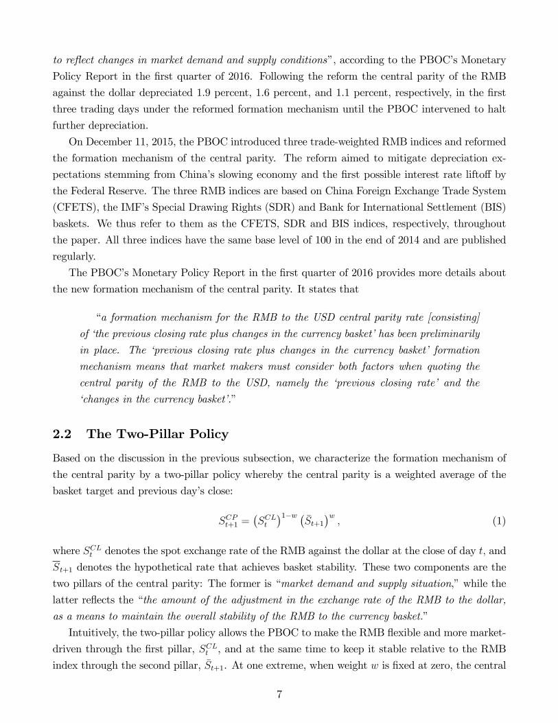
2.2 The Two-Pillar Policy
Based on the discussion in the previous subsection, we characterize the formation mechanism of
the central parity by a two-pillar policy whereby the central parity is a weighted average of the
basket target and previous day’s close:
SCPt+1 =(SCLt
)1−w (St+1
)w, (1)
where SCLt denotes the spot exchange rate of the RMB against the dollar at the close of day t, and
St+1 denotes the hypothetical rate that achieves basket stability. These two components are the
two pillars of the central parity: The former is “market demand and supply situation,”while the
latter reflects the “the amount of the adjustment in the exchange rate of the RMB to the dollar,
as a means to maintain the overall stability of the RMB to the currency basket.”
Intuitively, the two-pillar policy allows the PBOC to make the RMB flexible and more market-
driven through the first pillar, SCLt , and at the same time to keep it stable relative to the RMB
index through the second pillar, St+1. At one extreme, when weight w is fixed at zero, the central
7

parity is fully determined by the first pillar and is thus market driven to the extent that the
spot exchange rate is permitted to fluctuate within a band around the central parity rate under
possible interventions by the PBOC. At the other extreme, when weight w is fixed at 100 percent,
the central parity is fully determined by the second pillar; that is, the exchange rate policy is
essentially basket pegging and the RMB index does not change over time.
To explicitly represent the pillar associated with the currency basket St+1, we first discuss RMB
indices. In essence, an RMB index (e.g., CFETS) is a geometric average of a basket of currencies:
Bt = CB
(SCP,USD/CNYt
)wUSD (SCP,EUR/CNYt
)wEUR (SCP,JPY/CNYt
)wJPY· · · (2)
where CB is a scaling constant used to normalize the index level to 100 in the end of 2014,
SCP,i/CNYt denotes the central parity rate in terms of the RMB for the currency i in the basket,
and wi the corresponding weight for i = USD, EUR, JPY , etc. When the RMB strengthens (or
weakens) relative to the currency basket, the RMB index goes up (or down).
The key central parity rate is the one of the RMB against the dollar, denoted as SCPt ≡1/S
CP,USD/CNYt . According to the PBOC, once SCPt is determined, the central parity rates for
other non-dollar currencies are determined as the cross rates between SCPt and the spot exchange
rates of the dollar against those currencies. Therefore, we focus on the formation mechanism of
the central parity rate SCPt . For this reason, we refer to it simply as the central parity wherever
there is no confusion.
The RMB index can be rewritten in terms of the central parity rate of the RMB against the
dollar, SCPt , and a dollar index of all the non-RMB currencies, Xt:
Bt = χX1−wUSDt
SCPt, (3)
where Xt denotes the index-implied dollar index, defined by
Xt ≡ CX
(SCP,EUR/CNYt
SCP,USD/CNYt
) wEUR1−wUSD
(SCP,JPY/CNYt
SCP,USD/CNYt
) wJPY1−wUSD
· · · (4)
with a scaling constant CX , and χ ≡ CB/C1−wUSDX . The scaling constant CX is chosen such that
Xt coincides in the end of 2014 with the well known U.S. Dollar Index that is actively traded on
the Intercontinental Exchange under ticker “DXY”. We construct the index-implied basket Xt
based on equation (4) (see the online appendix for details). Note that the composition for the
CFETS and SDR indices has changed since 2017. Take the CFETS index as an example. On
December 29, 2016, the PBOC decided to expand the CFETS basket from 13 currencies to 24
currencies and at the same time reduced the dollar’s weight from 26.4 percent to 22.4 percent. We
take into account the composition changes of RMB indices when we construct Xt (please see the
8

online appendix for details). The index-implied dollar basket Xt, plotted in Figure 2, is shown to
be highly correlated with the U.S. dollar index DXY.
Figure 2: Index-implied Dollar Basket vs. DXY
In this figure we plot the historical dollar index (black dotted line) together with the dollar baskets
implied in three indices. The dollar basket implied in the CFETS (respectively, SDR or BIS) index is
plotted using blue solid line (respectively, red dashed or green dash-dot lines).
15Jan 15May 15Sep 16Feb 16Jun 16Oct 17Mar 17Jul 17Nov 18Apr 18Aug 18Dec88
90
92
94
96
98
100
102
104
106CFETS XSDR XBIS XDXY
The pillar St+1 is determined so as to achieve basket stability. Put differently, it is the value
that would keep the RMB index unchanged if the central parity were set at such value. Therefore
it is straightforward to show8
St+1 = SCPt
(Xt+1
Xt
)1−wUSD. (5)
The expression of St+1 in equation (5) is intuitive. The key idea is that movements in the RMB
index are attributable to movements in either the value of the RMB relative to the dollar, or
the value of the dollar relative to the basket of non-dollar currencies in the RMB index, or both.
The relative contributions of these two types of the movements are determined by wUSD and
(1− wUSD), respectively. As a result, in order for the RMB index to remain unchanged in response
to movement in the dollar index, hypothetically, the value of the RMB relative to the dollar should
be at a level that exactly offsets such movement.
8Specifically, the expression of St+1 can be derived as follows. At time t, the RMB index is given by Bt =
χX1−wUSDt
SCPt. At time t + 1, if the index-implied dollar baset changes its value to Xt+1, the RMB index would
become Bt+1 = χX1−wUSDt+1
SCPt+1if the central parity were set as SCPt+1. Equalizing Bt and Bt+1 (i.e., Bt = χ
X1−wUSDt
SCPt=
χX1−wUSDt+1
SCPt+1) determines the hypothetical value of SCPt+1, or St+1, which would keep the RMB index unchanged.
9

Substituting the above equation into equation (1), the two-pillar policy can be described by
the following equation:
SCPt+1 =(SCLt
)(1−w)
[SCPt
(Xt+1
Xt
)1−wUSD]w
. (6)
In the following subsection we empirically test and present empirical evidence for the above for-
mulation.
2.3 Empirical Evidence
We document here that the RMB central parity has closely tracked our equation (1) summarizing
the offi cial policy statements. In addition, we find strong empirical support for a central parity
rule that gives equal weights to each of the two pillars (i.e., w = 1/2).
To empirically test the two-pillar formulation in equation (1), we run the following regression:
log
(SCPt+1
SCPt
)= α · log
(SCLtSCPt
)+ β · (1− wUSD) log
(Xt+1
Xt
)+ εt+1. (7)
That is, the daily change in the log central parity (i.e., log(SCPt+1/S
CPt
)is regressed on the two
pillars scaled by the previous central parity (i.e., log(SCLt /SCPt
)and (1− wUSD) log (Xt+1/Xt)).
The coeffi cients α and β correspond to 1−w and w, respectively. The R-squared of the regressionis a good indicator of the extent to which the actual formation mechanism of the central parity
can be explained by our formulation of the two-pillar policy.
The results from the regression (7) for the whole sample period are reported under Column
“Whole Sample”in Panel A of Table 1. The regression results support that w = 1/2 as both of the
coeffi cients α and β are roughly equal to one half. The PBOC’s Monetary Policy Report in the first
quarter of 2016 has an example that seems to suggest equal weights for both pillars. Consistent
with the report, our empirical analysis provides supportive empirical evidence for w = 1/2 for
the period following December 11, 2015 when the RMB indices were announced for the first time.
Moreover, the regression has a very high R-squared at around 80 percent, which suggests that
our formulation of the two-pillar policy has a large explanatory power in describing the formation
mechanism of the central parity in practice.
Next, we show that the above results also largely hold after a new “countercyclical factor”was
introduced in the formation mechanism of the central parity. Specifically, the PBOC confirmed on
May 26, 2017 that it had modified the formation mechanism of the central parity by introducing
the new countercyclical factor, although no detailed information has been disclosed about how the
countercyclical factor is constructed.9 The modification is believed to “give authorities more control
9See the statement on the CFETS website: http://www.chinamoney.com.cn/fe/Info/38244066.
10

over the fixing and restrain the influence of market pricing.”10 The policy change is perceived by
many market participants as a tool to address depreciation pressure without draining foreign
reserves. However, it undermines earlier efforts to make the RMB more market driven. The
countercyclical factor was then subsequently removed as reported by Bloomberg on January 9,
2018. It signals the return to the previous two-pillar policy. The removal of the countercyclical
factor in January 2018 reflects the RMB’s strength over the past year as well as the dollar’s
protracted decline.
Accordingly we divide the whole sample period into three subsample periods: regime 1 (12/11/2015
to 5/25/2017), regime 2 (5/26/2017 to 1/8/2018), and regime 3 (1/9/2018 to 12/31/2018).11
Loosely speaking, regimes 1 and 3 refer to the subperiods without the countercyclical factor, while
regime 2 represents the subperiod when the countercyclical factor was added to the determination
of the central parity. The regression results for these three subsample periods are reported under
Columns “Regime 1”, “Regime 2”, and “Regime 3”in Table 1, respectively.
Table 1: Empirical Evidence for the Two-Pillar PolicyPanel A: Unconstrained Regressions
Whole Sample Regime 1 Regime 2 Regime 3
α β R2 α β R2 α β R2 α β R2
CFETS 0.53 0.47 0.81 0.49 0.51 0.82 0.53 0.40 0.78 0.57 0.40 0.81
SDR 0.55 0.45 0.80 0.49 0.49 0.80 0.53 0.40 0.79 0.60 0.40 0.81
BIS 0.55 0.42 0.78 0.51 0.48 0.78 0.52 0.40 0.79 0.61 0.30 0.79
Panel B: Constrained Regressions
Whole Sample Regime 1 Regime 2 Regime 3
α β R2 α β R2 α β R2 α β R2
CFETS 0.53 0.47 − 0.49 0.51 − 0.55 0.45 − 0.58 0.42 −SDR 0.55 0.45 − 0.51 0.49 − 0.56 0.44 − 0.60 0.40 −BIS 0.57 0.43 − 0.52 0.48 − 0.55 0.45 − 0.64 0.36 −
Notes: This table reports the results of regression (7) in which the daily change in the log central
parity (i.e., log(SCPt+1/S
CPt
)is regressed on the two pillars scaled by the previous central parity (i.e.,
log(SCLt /SCPt
)and (1− wUSD) log (Xt+1/Xt)). The results of unconstrained (constrained) regressions
are reported in Panel A (Panel B). The regression is conducted in four different periods: whole sam-
ple period (12/11/2015 to 12/31/2018), regime 1 (12/11/2015 to 5/25/2017), regime 2 (5/26/2017 to
1/8/2018), and regime 3 (1/9/2018 to 12/31/2018). All regression coeffi cients are statistically significant
at the 99 percent level.
10See the article “China Considers Changing Yuan Fixing Formula to Curb Swings”on Bloomberg News on May25, 2017.11We are grateful to an anonymous referee for suggesting the empirical analysis over these three subsample
periods.
11

Compared to the results in Column “Whole Sample”, the results in Column “Regime 1”pro-
vide even stronger empirical evidence for our two-pillar policy formulation in that the regression
coeffi cients α or β are even closer to 0.5 with slightly higher R-squared. The stronger results in
this subperiod are intuitive, because presumably this is the subperiod when the two-pillar policy
holds as closest as possible to our formulation.12 As a result of the introduction of the counter-
cyclical factor, the R-squared in Column “Regime 2”slightly decreases, but remains large around
80 percent. Once the countercyclical factor was reportedly dropped, the R-squared in Column
“Regime 2”increases.
The results reported in Panel A of Table 1 are from unconstrained regressions whereby we do
not impose the restriction that the coeffi cients sum up to one. Interestingly, the regression results
suggest it roughly holds in the data (i.e., α + β ≈ 1). We also run constrained regressions by
explicitly imposing the above restriction. The results are reported in Panel B of Table 1. The
constrained regression results lend further support for w = 1/2.
Figure 3: Empirical Evidence for the Two-Pillar Approach
This figure plots the coeffi cients β from 60-day rolling-window regressions: logSCPt+1
SCPt= α · log
SCLtSCPt
+
β ·(1− windUSD
)log
Xindt+1
Xindt
+ εt+1, where superscript “ind”indicates one of the three indices CFETS (blue
solid line), BIS (red dashed line), and SDR (green dash-dot line).
15Dec 16Mar 16Jul 16Nov 17Feb 17Jun 17Oct 18Jan 18May 18Sep 18Dec0
0.1
0.2
0.3
0.4
0.5
0.6
0.7
0.8
0.9
160day RollingRegression Coefficient (w)
CFETSSDRBIS
The above results from running the regression in equation (7) shed light on the average weights
on the two pillars during a fixed period, but are silent about possible time variation in the weights.12Note that the PBOC also changed the composition of the CFETS basket in the subperiod “regime 1”. The
new CFETS basket, effective January 1, 2017 includes 13 additional currencies and puts lower weight on the dollar.The adjustment is considered as a signal that the PBOC is likely to maintain the same formation mechanism of thecentral parity on a trade-weighted basis. In unreported results, we show that focusing on the subperiod betweenJanuary 1, 2017 and May 25, 2017, the R-squared from the same regression increases to 86% for the CFETS index.
12

To further investigate how the weights may possibly vary over time, we run the above regression
by using 60-day rolling windows, starting from 60 business days after August 11, 2015. Figure 3
plots the estimate of weight w implied by the rolling-window regressions.
Figure 3 shows that the weight w is initially around 0.1 in the period prior to the introduction
of the RMB indices. The results suggest that the formation mechanism before December 2015
follows closer to a “one-pillar”policy in the sense that it is almost completely determined by the
previous day’s close as the dollar basket implied in the RMB index carries very little weight.13
After the RMB indices were introduced on December 11, 2015, the weight w has since then steadily
increased and stabilized around 0.5, suggesting that the two-pillar policy with equal weights is in
place. Since May 2017 when a countercyclical factor was introduced, the estimate of weight w
exhibits more variability under the modified two-pillar policy with the new countercyclical factor.
2.3.1 Robustness Checks
Lastly we conduct robustness checks by taking into account another modification of the two-pillar
policy: On February 20, 2017, the PBOC reduced the reference period for the central parity
against the RMB index from 24 hours to 15 hours. According to Monetary Policy Report in the
second quarter of 2017, the rational for the adjustment is to avoid “repeated references to the daily
movements of the USD exchange rate in the central parity of the following day”since the previous
close has already incorporated such information to a large extent. This adjustment, however, is
widely believed to have limited impact on the RMB exchange rate. Accordingly, we repeat the
above empirical analysis for two subsample periods: “Subsample I” (12/11/2015 to 2/19/2017)
when a 24-hour reference period was used, and “Subsample II”(2/20/2017 to 12/31/2018) when
a 15-hour reference period was used.
To carry out the analysis, it is important to point out some subtle issues about timing. First,
the spot rate SCLt in equation (7) is the rate at the closing time 5PM New York time or 5AM
Beijing time of the next day (or 6AM if not in daylight saving time). To clarify, we denote it
SCLt+1,5AM in Beijing time by adding the time stamp in the subscript. Similarly, we denote the
central parity at date t + 1 by SCPt+1,9:15AM . Second, even though the central parity SCPt+1,9:15AM
is announced at 9:15AM of date t + 1, it is unclear which 24-hour reference period is used in
evaluating the changes in the basket. For now, we denote it by log (Xt+1,9:15AM/Xt,9:15AM). Using
high-frequency data we will identify the 24-hour reference period shortly. In the end, we can
rewrite the regression (7) below in terms of Beijing time:
logSCPt+1,9:15AM
SCPt,9:15AM
= α · logSCLt+1,5AM
SCPt,9:15AM
+ β · (1− wUSD) logXt+1,9:15AM
Xt,9:15AM
+ εt+1. (8)
13This finding is consistent with the regression results, reported in the online appendix, for the period betweenAugust 11, 2015 and December 10, 2015 that the regression-based estimate of w is close to zero and the R-squaredis very high (around 0.95) for this period.
13

To cope with the subtle timing issues, we use Bloomberg BFIX intraday data, which are
available every 30 minutes on the hour and half-hour throughout the day. Based on the BFIX
data, we can thus construct the index-implied dollar basket Xt and the spot rate SCLt for all
48 half-hour intervals throughout the day.14 As shown in the online appendix, we find strong
empirical evidence that the formation mechanism of the central parity in Subsample (I) uses the
24-hour reference period starting from 7:30AM to 7:30AM the next day, and the spot rate at
4:30PM close. We also find evidence for the (overnight) 15-hour reference period starting 4:30PM
to 7:30AM the next day for Subsample (II).
Table 2: Empirical Evidence for the Two-Pillar Policy: Robustness Checks
Panel A: Unconstrained Regressions
Subsample I Subsample II
α β R2 α β R2
CFETS 0.56 0.64 0.82 0.74 0.71 0.86
SDR 0.57 0.58 0.76 0.74 0.61 0.85
BIS − − − − − −Panel B: Constrained Regressions
Subsample I Subsample II
α β R2 α β R2
CFETS 0.41 0.59 − 0.59 0.41 −SDR 0.46 0.54 − 0.60 0.40 −BIS − − − − − −
Notes: We use intraday Bloomberg BFIX data to run regressions (9) and (10). The results of uncon-
strained (constrained) regressions are reported in Panel A (Panel B). Column “Subsample I” reports
the results from the regression (9) for Subsample period I (12/11/2015 to 2/19/2017) when the 24-hour
reference period starting from 7:30AM to 7:30AM the next day is used. Column “Subsample II”reports
the results from the regression (10) for Subsample period II (2/20/2017 to 12/31/2018) when the 15-hour
reference period starting from 4:30PM to 7:30AM the next day is used. All regression coeffi cients are
statistically significant at the 99 percent level.
Consequently, using Bloomberg BFIX intraday data, we conduct the empirical tests of the
two-pillar policy based on the following two regressions:
log
(SCPt+1,9:15AM
SCPt,9:15AM
)= α · log
(SCLt,4:30PM
SCPt,9:15AM
)+ β · (1− wUSD) log
(Xt+1,7:30AM
Xt,7:30AM
)+ εt+1, (9)
14Because Bloomberg has stopped producing the BFIX data for Venezuela currency, we do not construct intradayspot fixings for the BIS index.
14

and
log
(SCPt+1,9:15AM
SCPt,9:15AM
)= α · log
(SCLt,4:30PM
SCPt,9:15AM
)+ β · (1− wUSD) log
(Xt+1,7:30AM
Xt,4:30PM
)+ εt+1. (10)
We run the regression (9) using the 24-hour reference period for the relevant subperiod “Subsample
I”. Similarly, we run the regression (10) using the 15-hour reference period for the relevant
subperiod “Subsample II”. The results are reported in Columns “Subsample I”and “Subsample
II”, respectively, in Table 2.
Consider the unconstrained regression results in Panel A of Table 2. As before, the results
suggest that the coeffi cients α and β are roughly equal, although they do not add up to one in the
unconstrained regressions. The R-squared range from 76 percent to 86 percent, suggesting that
our two-pillar policy does a good job of characterizing the formation mechanism of the central
parity in practice. The constrained regression results in Panel B of Table 2 lend further support
to the findings.
2.4 Analysis of the Two-Pillar Policy Using Derivatives Data
We have shown that China’s exchange rate policy since December 2015 can be characterized with
the two-pillar policy. The regression results in the previous subsection provide strong empirical
evidence for such policy and suggest that the two pillars carry about the same weights. In this
subsection, using derivatives data from the lens of a reduced-form no-arbitrage model, we analyze
how the financial market participants assess the two pillar policy. A priori, it is unclear whether
the actual policy, characterized by our two-pillar formulation, is optimal or sustainable from the
viewpoint of investors. We will turn to a formal theoretical model to study and evaluate the
optimality of the two-pillar policy in Section 3 where the government’s objective is explicitly
modeled. In this subsection, we empirically assess financial market participants’view about the
policy.
In particular, building on Jermann (2017), we assume that there is a probability p that the
two-pillar policy regime continues, and a probability (1− p) that the policy ends tomorrow. Ifit ends, the exchange rate equals the fundamental exchange rate Vt that is arbitrage-free itself,
satisfying1 + r$
1 + rCEQt [Vt+1] = Vt. (11)
The interpretation of Vt can be quite broad; for example, we can interpret it as the exchange rate
that would prevail when the RMB had become freely floating.
15

The equilibrium exchange rate St is given by
St =1 + r$
1 + rC
[pEQ
t H(St+1, S
CPt+1, b
)+ (1− p)EQ
t Vt+1
](12)
=1 + r$
1 + rCpEQ
t H(St+1, S
CPt+1, b
)+ (1− p)Vt,
where b denotes the width of the trading band around the central parity,
H(St+1, S
CPt+1; b
)= max
(min
(St+1, S
CPt+1 (1 + b)
), SCPt (1− b)
), (13)
and EQt [·] refers to expectations under the RMB risk-neutral measure, and r$ and rC are per-
period interest rates in the U.S. and China, respectively. Intuitively, the current spot rate is the
expected value of the exchange rate in the two regimes, appropriately adjusted for the yields.
If the equilibrium exchange rate St falls within the band around the central parity, the observed
spot exchange rate at the close is equal to St. Otherwise, the spot exchange rate is equal to Sttruncated at the (lower or upper) boundary of the band. Therefore, the model-implied spot
exchange rate at the close then equals
SCLt = H(St, S
CPt ; b
). (14)
Next, we turn to the formation mechanism of the central parity SCPt . To make the model
tractable enough for estimation, we consider the following two-pillar rule, which represents a
good approximation of the two-pillar policy empirically and is also consistent with the formation
mechanism of the central parity in the PBOC’s report in the broad sense. Specifically, we replace
the previous close by SCPt (Vt+1/Vt)γ, 0 ≤ γ ≤ 1, while keeping the basket pillar unchanged. That
is, the two-pillar rule is modeled as the following:
SCPt+1 =
[SCPt
(Vt+1
Vt
)γ]1−w[SCPt
(Xt+1
Xt
)(1−wUSD)]w
≡ SCPt
(Vt+1
Vt
)α(Xt+1
Xt
)β, (15)
where α ≡ γ (1− w) and β ≡ (1− wUSD)w are some constants bounded between 0 and 1.
The reduced-form model is particularly tractable in continuous time. We show in Appendix B1
that the equilibrium exchange rate St has a closed-form solution in continuous time. Specifically,
denote by St ≡ St/SCPt the equilibrium exchange rate St scaled by the central parity SCPt , and
denote by Vt ≡ Vt/SCPt the scaled fundamental exchange rate. In Proposition 4 in Appendix B1,
we prove that the scaled equilibrium exchange rate can be expressed as a univariate function S (·)of the scaled fundamental exchange rate (i.e., St = S(Vt)), and characterize the solution in closed
16

form. Figure 4 plots the scaled equilibrium exchange rate S(Vt).
Figure 4: Equilibrium Exchange Rate S(Vt)
This figure plots in solid line the scaled equilibrium exchange rate S(V ) as a function of V .
As shown in Figure 4, there exist two thresholds V∗ and V ∗ within which the function S(Vt) has
a S shape. When Vt hits the threshold V∗ or V ∗, the equilibrium exchange rate St breaches either
the lower boundary (i.e., SCPt (1− b)) or the upper boundary (i.e., SCPt (1 + b)) of the trading
band. When Vt is suffi ciently away from both thresholds, the equilibrium exchange rate would
change almost one for one in response to changes in the fundamental exchange rate. However,
when Vt gets closer to one of the thresholds, government intervention becomes increasingly likely.
As a result, the equilibrium exchange rate becomes less sensitive to the fundamental value– a
flatter slope of the function S(Vt) near the boundaries of the trading band. This is reminiscent of
the exchange rate behavior in a target zone model (see Krugman (1991)) that the expectation of
possible intervention affects exchange rate behavior even when the exchange rate lies inside the
zone (the so-called “honeymoon effect”). The honeymoon effect implies that the spot exchange rate
varies less than the underlying fundamental value. Our estimation explicitly takes into account
the non-linear relationship between the observed spot exchange rate and the fundamental value.
We estimate the model to match the closing spot exchange rate and four RMB option prices.
We assume that the options market is free of government interventions. The model-implied price
of a call option with maturity τ and strike K is given by
C (K; τ) = e−rCNY τ(pτEQ
[max
(H(St+τ , S
CPt+τ , b
), K)]
+ (1− pτ )EQ [max (Vt+τ , K)]). (16)
The price of a put option can be represented in a similar way. The special case with zero trading
bandwidth (i.e., b = 0) is tractable and has closed-form option pricing formula (see the online
17

appendix). However, in the general case with a nonzero trading bandwidth we obtain option
prices numerically by simulation.
We estimate (V, p, σV ) for each day in the sample period between December 11, 2015 and
December 31, 2018. The beginning date of the sample period is chosen as December 11, 2015
because the RMB indices were introduced on that date for the first time. During this period, the
trading bandwidth is offi cially 2 percent. However, the effective width is much smaller, around
0.5%. As a result, we choose b = 0.5% in estimating the model.15 To simplify the estimation, we
fix ρ = 0. The parameter γ determines how sensitive the central parity is to the changing market
conditions. We choose γ = 1/4 so that the frequency of the pillar, SCPt (Vt+1/Vt)γ, staying within
the trading band is roughly similar to that of the close SCLt .
Figure 5: Baseline Parameter Estimates
This figure reports the results of the baseline estimation. In the top panel, we plot the fundamental
exchange rate Vt (blue solid line), the central parity (red dashed line), and the close (black dashed line).
In the middle panel, we plot the probability of the policy still being in place three months later pt. In
the bottom panel, we plot the fundamental exchange rate volatility σV (blue solid line), and the average
implied volatilities of 10-delta options (red dashed line) and 25-delta options (black dashed line).
15Dec 16Mar 16Jun 16Oct 17Jan 17May 17Aug 17Nov 18Mar 18Jun 18Sep 18Dec
6.5
7
15Dec 16Mar 16Jun 16Oct 17Jan 17May 17Aug 17Nov 18Mar 18Jun 18Sep 18Dec0.2
0.4
0.6
0.8
15Dec 16Mar 16Jun 16Oct 17Jan 17May 17Aug 17Nov 18Mar 18Jun 18Sep 18Dec
0.1
0.2
Figure 5 displays the main estimation results. As shown in the top panel, the fundamental
exchange rate Vt is estimated to be always greater than both the central parity and spot rates,
consistent with depreciation expectations. Implied from the estimate of Vt, the RMB is valued on
average about 1.7 percent higher than its fundamental value during the whole sample period. The
gap between the spot rate and the estimated fundamental value is particularly elevated in the first
15The results for the case of b = 2%, unreported here, are similar and available upon request.
18

couple of months of the sample period, ranging between 2 percent and 9 percent. The large gap
in the early sample period is consistent with the expectation of 10-15 percent depreciation of the
RMB.16 It is possible that the PBOC may intervene in both spot and derivatives markets, which
may contribute to the overall small deviations between the estimated fundamental exchange rate
and the spot rate.17 In the next subsection we extend the reduced-form model to the offshore
market and provide more discussion on the impact of government intervention.
The middle panel in Figure 5 plots the probability that the current policy would still be in
place three months later. It suggests that financial markets attached a high probability to the
policy still being in place three months later. The estimated probability of policy continuation
fluctuates mostly between 60 percent and 90 percent. In particular, until the countercyclical factor
was introduced in May 2017, the average probability of policy continuation is about 76 percent.
These findings lend further support to the validity of the two-pillar policy we have formulated.
At the same time our estimation results capture some episodes when financial market partic-
ipants cast doubt on the sustainability of the two-pillar policy. For example, the model-implied
probability of policy continuation drops to the lowest level, around 15 percent, on May 23, 2017
in the week preceding the PBOC’s confirmation of adding the new countercyclical factor on May
26, 2017. On January 9, 2018, the PBOC has reportedly removed the countercyclical factor.18 As
a result of the return to the two-pillar policy, the probability of policy continuation has since then
increased and stabilized around the average level of 60 percent. Overall, our findings suggest that
financial market participants have relatively high confidence in the continuation of the two-pillar
policy.
The implied volatility of the fundamental exchange rate shown in the bottom panel of Figure
5 displays a relatively stable pattern in that the implied volatility fluctuates around its average
value 8.6 percent during the whole sample period. It is worthwhile to point out that since the
U.S. presidential election, the implied volatility has steadily decreased from around 14 percent in
mid-December of 2016 to only 4 percent in the end of May, 2017. It suggests “damping currency
volatility against the dollar [is] now a bigger priority.”19
16See, for example, the Reuters article “Pressure on China central bank for bigger yuan depreciation”on January7, 2016.17Consistent with this possibility, we find that the difference between onshore and offshore exchange rates– a
gauge for the effect of the government intervention– explains about 5 percent of the variation in the fundamentalvalue scaled by the central parity. This result, unreported but available upon request, also suggests that ourfundamental value estimate contains useful information beyond the aforementioned difference.18See the article “China Changes the Way It Manages Yuan After Currency’s Jump” on Bloomberg News on
January 9, 2018.19See, for example, the article “China Hitches Yuan to the Dollar, Buying Rare Calm”in the Wall Street Journal
on May 25, 2017.
19
2.4.1 Offshore RMB Market
The RMB trades in both onshore (i.e., mainland China) and offshore (e.g., Hong Kong) markets.
We extend the reduced-form model to incorporate the joint dynamics between these markets. For
greater specificity, we use “CNY”and “CNH”to denote RMB-denominated accounts that trade
in onshore and offshore markets, respectively. Similarly, we use “USDCNY”and “USDCNH”to
denote the exchange rates of the CNY and the CNH against the USD, respectively. The CNH-
CNY basis– the spread between USDCNH and USDCNY– has remained fairly narrow. 20 The
small deviations between these two exchange rates also reflect the rising integration of onshore
and offshore RMB markets following a series of recent developments.21
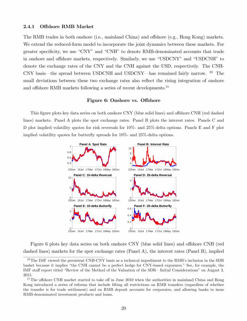
Figure 6: Onshore vs. Offshore
This figure plots key data series on both onshore CNY (blue solid lines) and offshore CNH (red dashed
lines) markets. Panel A plots the spot exchange rates. Panel B plots the interest rates. Panels C and
D plot implied volatility quotes for risk reversals for 10%- and 25%-delta options. Panels E and F plot
implied volatility quotes for butterfly spreads for 10%- and 25%-delta options.
15Dec 16Jul 17Mar 17Oct 18May 18Dec
6.4
6.6
6.8
7Panel A: Spot Rate
15Dec 16Jul 17Mar 17Oct 18May 18Dec
4
6
8
10Panel B: Interest Rate
15Dec 16Jul 17Mar 17Oct 18May 18Dec0
5
10Panel C: 10delta Reversal
15Dec 16Jul 17Mar 17Oct 18May 18Dec0
2
4
Panel D: 25delta Reversal
15Dec 16Jul 17Mar 17Oct 18May 18Dec0
1
2
Panel E: 10delta Butterfly
15Dec 16Jul 17Mar 17Oct 18May 18Dec0
0.2
0.4
0.6Panel F: 25delta Butterfly
Figure 6 plots key data series on both onshore CNY (blue solid lines) and offshore CNH (red
dashed lines) markets for the spot exchange rates (Panel A), the interest rates (Panel B), implied
20The IMF viewed the persistent CNH-CNY basis as a technical impediment to the RMB’s inclusion in the SDRbasket because it implies “the CNH cannot be a perfect hedge for CNY-based exposures.”See, for example, theIMF staff report titled “Review of the Method of the Valuation of the SDR– Initial Considerations”on August 3,2015.21The offshore CNH market started to take off in June 2010 when the authorities in mainland China and Hong
Kong introduced a series of reforms that include lifting all restrictions on RMB transfers (regardless of whetherthe transfer is for trade settlement) and on RMB deposit accounts for corporates, and allowing banks to issueRMB-denominated investment products and loans.
20

volatility quotes for risk reversals (Panels C and D, respectively) and butterfly spreads (Panels
E and F, respectively) for 10%- and 25%-delta options. Panel A of Figure 6 confirms that the
onshore and offshore spot rates tend to move in lockstep. The last four panels show that CNY
or CNH options have similar prices. As shown in Panel B, the interest rates on these markets
occasionally diverge due to the PBOC’s intervention.
The PBOC can directly intervene in the offshore spot or forward/swap markets, besides capital
controls that limit the RMB flow between the onshore and offshore markets.22 For the former spot-
market intervention, the PBOC can use nonsterilized foreign exchange intervention, for example,
to support the CNH by permanently repatriating CNH to mainland China. The cost of such
intervention is the immediate run-down of foreign reserves. For instance, offshore PBOC agent
banks were believed to have intervened heavily in the spot CNH market, causing the offshore
interest rate to sharply rise to more than 10 percent in mid January 2016.23
On the other hand, the authorities may also intervene in the offshore forward and swap mar-
kets.24 Forward market intervention through selling-USD-buying-CNH forwards strengthens the
CNH because of the covered interest parity; that is, it puts downward pressure on the USDCNH
forward rate, mechanically causing the CNH to appreciate against the USD under the covered
interest parity. Compared to the spot market intervention, forward market intervention avoids
immediately draining foreign reserves.
In the aftermath of the August 2015 devaluation, Chinese commercial banks in Hong Kong
acting as agents for the PBOC started intervening in the offshore foreign exchange forward/swap
markets. According to the public data on its derivatives holdings disclosed by the PBOC for the
first time on March 31, 2016, the central bank held a nominal short position of $28.9 billion in
forwards as of February 29, 2016.25 From the same data, the PBOC increased its short position to
$45.3 billion in September 2016, indicating another round of intervention in the offshore forward
market. The forward market intervention drove up the CNH interest rate in September as shown
in Panel B. Later in January and May 2017 the settlement of these forward transactions caused the
CNH interest rate to spike again because the counterparty side of the intervention (e.g., investors)
had to source CNH for delivery to the agent banks who in turn repatriate the CNH to the PBOC.26
22Arguably, the PBOC could also intervene in the options market in theory. For example, through the put-callparity relationship, the options intervention may impact the forward rate. However, the PBOC can achieve thesame effect by intervening directly in the forward market. The PBOC’s derivatives holdings data (discussed below)shows that the PBOC had zero position in options during the period when the data was available.23In January 2016, the CNH was significantly weaker than the CNY amid short selling pressure under the
expectations of another imminent devaluation. The elevated implied volatilities for risk reversals in January 2016,shown in Panels C and D of Figure 7, also indicate strong speculative bets on RMB depreciation.24See, for example, a Wall Street Journal article on August 27, 2015, titled “PBOC Uses Unusual Tool to Tame
Yuan Fall Expectations.”25The same data, however, shows that the PBOC had zero positions in options, signaling no direct intervention
in the options market.26Our analysis of the PBOC’s derivatives holdings data suggests that as of February 29, 2016 the Chinese central
bank held $28.9 billion short position of forwards at the tenor of around one year, and in September increased theshort position to $45 billion by shorting additionally $10 billion forward at the tenor of around six months and $6
21

In this way, CNH liquidity is reduced in a similar manner as nonsterilized interventions.
We extend the reduced-form model to incorporate the joint dynamics of the onshore and
offshore markets. Suppose the cost of arbitraging between these markets is c ≥ 0. We assume that
the onshore spot rate, SCLt , serves as the “underlying anchor”for the offshore spot rate, denoted
TCLt . Specifically, if we let Tt denote the equilibrium exchange rate for the offshore CNH market,
then the offshore spot rate TCLt is given by
TCLt = H(Tt, S
CLt ; c
)= max
(min
(Tt, S
CLt (1 + c)
), SCLt (1− c)
),
Similarly as the onshore CNY market, the equilibrium exchange rate for the offshore market, Tt,
satisfies the following no-arbitrage condition
Tt =1 + r$
1 + roffshorepEQ
t H(Tt+1, S
CLt+1; c
)+ (1− p) 1 + r$
1 + rCEQt Vt+1 (17)
=1 + r$
1 + roffshorepEQ
t H(Tt+1, S
CLt+1; c
)+ (1− p)Vt,
where roffshoret denotes the offshore interest rate for CNH deposits (i.e., HIBOR rate). We solve and
estimate the model in continuous time and set c = 0.5% to be the same as the trading bandwidth.
The equilibrium exchange rate Tt is a solution to an ordinary differential equation with free
boundaries. Because of no closed-form solution, we numerically solve the free-boundary problem
using the finite-difference method. The detailed derivation as well as numerical methodology are
delegated to Appendix B2.
Figure 7 plots the estimation results based on data on both offshore and onshore markets
(particularly, the CNH options data). As shown in the figure, the estimation results for the
fundamental exchange rate (top panel), the probability of policy continuation (middle panel), and
the volatility of the fundamental process (bottom panel) are very close to those in Figure 5 for
the onshore market. The similarity in the results is expected given the similar pricing of CNY
and CNH options. Furthermore, the PBOC’s intervention in the offshore market seems to work
through its impact on the offshore funding costs (e.g., spikes in the offshore interest rate as shown
in Panel B), which, however, has limited impact on our estimation results. The similarity in
the results further validates our reduced-form framework with the two-pillar policy as a plausible
approach to study both onshore and offshore RMB markets.
At this point we have empirically assessed financial market participants’view about the two-
pillar policy. We next turn to a formal theoretical model to study and evaluate the optimality of
the policy.
billion forwards at the tenor of around one year. These forward contracts started to mature in February throughMay 2017 according to the PBOC’s derivatives holdings data.
22

Figure 7: Offshore CNH Market Estimation Results
This figure reports the estimation results for both offshore (red dashed line) and onshore (blue solid
lines) markets. We plot the fundamental exchange rate Vt, the probability of the policy still being in
place three months later pt, and the fundamental exchange rate volatility σV in the top, middel, and
bottom panels, respectively.
15Dec 16Mar 16Jun 16Oct 17Jan 17May 17Aug 17Nov 18Mar 18Jun 18Sep 18Dec
6.46.66.8
77.2
15Dec 16Mar 16Jun 16Oct 17Jan 17May 17Aug 17Nov 18Mar 18Jun 18Sep 18Dec0.2
0.4
0.6
0.8
15Dec 16Mar 16Jun 16Oct 17Jan 17May 17Aug 17Nov 18Mar 18Jun 18Sep 18Dec
0.1
0.2
3 Theoretical Model
In this section, we develop a conventional flexible-price monetary model for exchange rate determi-
nation based on Svensson (1994).27 Our model extends the Svensson model along two important
dimensions. First, we incorporate the two-pillar policy and provide a theoretical microfoundation
for such policy in order to evaluate its optimality. Second, we further extend the model to examine
intraday government intervention.
3.1 Setup
There is an infinite number of periods with each period divided into two subperiods: “AM” and
“PM”. In each period, the government in the home country (China) chooses the optimal central
parity at subperiod AM, and the optimal monetary and exchange rate policies at subperiod PM.
Specifically, at the PM of each period, the government chooses the optimal level of money
stock for period t, denoted by mt, which then determines in equilibrium the domestic interest rate
it, and the exchange rate et under rational expectations. The money market equilibrium condition
27We are very grateful to the editor and the associate editor for very constructive suggestions that motivated usto develop the theoretical model for the RMB in this section.
23

for the home country links the logarithm of the money stock (mt) deflated by the logarithm of the
price level, pt, to the domestic interest rate, it, given by:
mt − pt = −αit. (18)
Assuming zero foreign exchange risk premium,28 the domestic interest rate satisfies the equilibrium
condition
it = i∗t + Et [et+1 − et] /∆t, (19)
where i∗t denotes the interest rate in the foreign country (the United States), and Et [·] denotesthe rational expectation. The log of the real exchange rate, qt, is given by
qt = p∗t + et − pt, (20)
where et denotes the spot exchange rate expressed in units of domestic currency (i.e., RMB) per
unit of foreign currency (i.e., USD). As normalization we set p∗t = 0.
At the AM of each period, the home country (indexed by N) trades with N other countries,
indexed by i = 0, · · · , N − 1. The U.S. is the numeraire country (indexed by 0), and countries
in the rest of the world (RoW) are indexed by 1 through N − 1. Assume that the price of each
country’s product is 1 in terms of its currency. Let R(i)t denote the price of currency i in dollars,
then country i’s product costs R(i)t dollar.
Through the balance-of-payments model in Flanders and Helpman (1979), we show that
if the government’s objective is solely minimizing the variability in the trade-balance growth,
then the optimal exchange rate policy is a basket peg (see Appendix C). Specifically, let ct ≡logS
CP,CNY/USDt denote the logarithm of the central parity SCP,CNY/USDt , and let TBt denote the
surplus in the home country’s balance of trade in terms of dollars defined as exports minus im-
ports. As shown in Appendix C, conditional on the observations of ∆ logR(i)t ≡ logR
(i)t /R
(i)t−1, for
i = 0, · · · , N − 1, minimizing the variability in the trade-balance growth, i.e., minct (∆ log TBt)2,
is equivalent to the following:
minct
(∑N−1i=1 ωi∆ logR
(i)t + ct−1 − ct
)2
,
where ωi denotes the weight of currency i in a currency basket. Note that by definition R(0)t is a
constant equal to one and thus is dropped from the above objective function. Under additional
simplifying assumptions, the optimal weights ωiN−1i=0 are shown to equal the share of country i in
the home country’s exports. The weight for the USD in the basket ω0 = 1−∑N−1
j=1 ωj is determined
28We will relax this assumption later in an extension of the model in which noise trading and intraday governmentintervention give rise to time-varying foreign exchange risk premium.
24

as well.29 Therefore, minimizing the variability in the trade-balance growth is equivalent to
minct
((1− ω0) ∆xt + ct−1 − ct)2 ,
where xt ≡ logXt denotes the logarithm of the basket-implied dollar index Xt. If the government
only cares about the stability of the trade-balance growth, the optimal exchange rate policy is
thus a basket peg, that is, ct = (1− ω0) ∆xt + ct−1, which is equal to the logarithm of the pillar
St in equation (5).
However, the government may also have other policy targets to meet in its objective function,
besides the stability of the trade-balance growth. For example, the government may want to
minimize the variability of the exchange rate (ct − et−1)2 or c2t , where et−1 denotes the logarithm
of the spot exchange rate expressed in units of the home currency per unit of numeraire currency
(in our case, the RMB against the USD).
Therefore, we extend Svensson (1994) to consider the following government’s objective func-
tion:30
E0
∞∑t=0
βt[ξdd
2t + ξii
2t + ξ∆x ((1− ω0) ∆xt −∆ct)
2 /∆t+ ξ∆e (ct − et−1)2 /∆t+ ξcc2t
]∆t, (21)
where dt ≡ et − ct denotes the exchange rate deviation relative to the central parity. The aboveobjective function implies suffi cient flexibility for the government to balance among the competing
targets of smoothing interest rate and stabilizing the exchange rate and the trade-balance growth.
3.2 The Government’s Problem
We now analyze and solve the government’s problem using dynamic programming. At the AM of
period t, the government observes the realization of∆xt, ct−1, dt−1, as well as other pre-determined
variables. We stack these state variables into the vector Yt =(∆xt, ct−1, qt−1, i
∗t−1,mt−1, dt−1, it−1
)′.
Let U (Yt) denote the government’s value function at the AM of period t, that is,
U (Yt) = mincs
EAMt
∞∑s=t
β(s−t)
[(ξdd
2s + ξii
2s) ∆t
+ξ∆x ((1− ω0) ∆xs −∆cs)2 + ξ∆e (cs − es−1)2 + ξcc
2s
], (22)
where EAMt [·] denotes the expectation conditional on the information set at the AM of period
t. Consistent with the data, we assume that the change in the basket-implied dollar index ∆xt
29Note that ω0 corresponds to ωUSD in the previous section, and the basket-implied dollar index (see (4) in the
previous section) is given by Xt ≡ CX∏N−1j=1
(R
(j)t
)− ωi1−ω0 .
30The model can be easily generalized to include more targets in the government’s objective function. In theonline appendix, we provide a generalized framework with additional targets such as ξ∆d (∆dt)
2/∆t, ξ∆i (∆it)
2/∆t,
ξuu2t/∆t from Svensson (1994).
25

follows an independent process across time:
∆xt = ε∆x,t,
where ε∆x,t follows a standard normal distribution with mean zero and variance σ2∆x∆t.
At the PM of period t, besides observing the central parity ct, the government also observes
the realizations of qt, i∗t , and other pre-determined variables, which are stacked into the vector:
Xt = (qt, i∗t ,mt−1, dt−1, it−1, ct)
′ .
Using dynamic programming, the government’s problem at PM has the following recursive for-
mulation:
V (Xt) = minut
(ξdd
2t + ξii
2t
)∆t+ βEPM
t [U (Yt+1)] , (23)
where ut ≡ mt − mt−1 denotes the change in the level of money supply, V (Xt) denotes the
government’s value function at the PM of period t, and EPMt [·] denotes the expectation conditional
on the information set at the PM of period t. The real exchange rate qt and the foreign interest
rate i∗t follows exogenous AR(1) processes:
qt =(1− ρq∆t
)qt−1 + εq,t,
i∗t = (1− ρi∗∆t) i∗t−1 + εi∗,t,
where εq,t ∼ N(0, σ2
q∆t)and εi∗,t ∼ N (0, σ2
i∗∆t) are independent and normally distributed shocks.
In the data, both processes are highly persistent with the AR(1) coeffi cients close to one.
The government’s problem at AM has a similar recursive formulation:
U (Yt) = minct
ξ∆x ((1− ω0) ∆xt −∆ct)2 + ξ∆e (ct − et−1)2 + ξcc
2t∆t+ EAM
t [V (Xt)] . (24)
The Bellman equations (23) and (24) constitute a standard linear-quadratic optimization prob-
lem. We show that the value functions U (Yt) and V (Xt) take a quadratic form
U (Yt) = (Y ′tUYt + U0) ∆t, (25)
V (Xt) = (X ′tV Xt + V0) ∆t,
where the coeffi cients U , U0, V , and V0 are determined endogenously.
3.3 Endogenous Two-Pillar Policy
We now solve the government’s problem at the AM period in (24) for the optimal formation
mechanism for the central parity. We decompose the state vector Xt into the vector of exogenous
26

shocks X(1)t = (qt, i
∗t )′, pre-determined variables X(2)
t = (mt−1, dt−1, it−1)′, and the endogenous
variable X(3)t = ct. The coeffi cient matrix V in the value function V (Xt) is also decomposed ac-
cordingly. Similarly, we decompose the state vector Yt into Y(1)t = (∆xt, ct−1)′, Y (2)
t =(qt−1, i
∗t−1
)′,
and Y (3)t = (mt−1, dt−1, it−1)′, and do the similar decomposition to U .
We can then solve the government’s problem in (24) for the optimal central parity rule. The
proposition below reports the result.
Proposition 1 Suppose the value function V (Xt) takes the quadratic form in (25), let Vcc ≡V (3,3), then the optimal central parity has the following two-pillar representation:
ct = w1et−1 + w2 (ct−1 + (1− ω0) ∆xt) + ht−1, (26)
where w1 ≡ ξ∆e/∆tVcc+ξc+(ξ∆e+ξ∆x)/∆t
, w2 ≡ ξ∆x/∆tVcc+ξc+(ξ∆e+ξ∆x)/∆t
, and ht−1 is related to the hedging demand.
Proof. See Appendix D1.The optimal central parity rule in equation (26) resembles the two-pillar policy we have for-
mulated. In particular, the first two terms correspond to the two pillars. The last term ht−1
represents the government’s hedging demand as the state of the economy varies over time. As
we will characterize the equilibrium more sharply, the hedging term ht−1 turns out to depend on
the lagged US interest rate only. Note that if the U.S. interest rate is independent over time,
the hedging term ht−1 is zero. Based on the calibrated parameter values, the hedging term is
small in magnitude. So the optimal central parity rule is primarily captured by our two-pillar
policy. In addition, we show below that when the government does not care about the interest
rate variability (i.e., ξi = 0), the hedging term is also zero because there is no longer demand for
hedging the foreign interest rate risk.
3.4 Optimal Monetary and Exchange Rate Policies
We now turn to the government’s optimization problem at the PM of period t. We focus on
discretionary policies where the central bank reoptimizes each period under discretion. As a
consequence, the interventions in each period will only depend on the predetermined variables in
that period. In particular, the exchange rate deviation from the central parity, i.e., dt = et−ct, is aforward-looking state variable. In a rational expectations equilibrium private agents’expectations
incorporate the restriction that the forward-looking variable dt is chosen as a function of the
predetermined variables Xt in that period. Formally, the restriction is
dt = DXt,
where the endogenous matrix D in our case is a 1 × 6 row vector. We focus on stationary
equilibriums.
27

We stack the state vector Xt and the forward-looking variable dt into the vector Zt. That is,
the first six elements of Zt is Xt and the last (seventh) element is dt. The transition equation can
be written as [Xt+1
Et [dt+1]
]= AZt +But + εZ,t+1, (27)
where εZ,t+1 ≡ (εq,t+1, εi∗,t+1, 0, 0, 0, w2 (1− ω0) ∆xt+1, 0)′ and the expressions for coeffi cients A and
B are given in (56) in Appendix D2.
Given the above linear transition equation, the government’s PM problem in (23) can be
rewritten as the following linear-quadratic problem:
1
∆tV (Xt) = min
utξdd
2t + ξii
2t + βEPM
t
[1
∆tU (Yt+1)
]= min
ut(X ′tQ
∗Xt +X ′tW∗ut + u′tW
∗′Xt + u′tR∗ut)
+β(X ′tQ
∗Xt +X ′tW∗ut + u′tW
∗′Xt + u′tR∗ut + U11V ar (∆x)
), (28)
where the expressions of coeffi cients (e.g., Q∗, Q∗, etc.) are given in Appendix D3. This is a
standard linear-quadratic problem to solve. Its solution is reported in the proposition below.
Proposition 2 In a stationary rational expectations equilibrium, the optimal monetary policy utsolves the problem in (28), given by
ut = −(R∗ + βR∗
)−1 (W ∗ + βW ∗
)′Xt ≡ −F ∗Xt, (29)
where F ∗ ≡(R∗ + βR∗
)−1 (W ∗ + βW ∗
)′. In equilibrium, the exchange rate deviation relative to
the central parity must satisfy
dt = HXt +Gut = (H −GF ∗)Xt ≡ DXt. (30)
The value function V (Xt) = (X ′tV Xt + V0) ∆t is determined where V0 = βU11V ar (∆x) and
V = Q∗ + βQ∗ −(W ∗ + βW ∗
)F ∗ − F ∗′
(W ∗ + βW ∗
)′+ F ∗′
(R∗ + βR∗
)F ∗.
Proof. See Appendix D3.
The above proposition together with Proposition (26) fully characterize the stationary equi-
librium. In the discretionary equilibrium with the rational-expectations restriction dt = DXt,
the transition equation in (27) implies that the exchange rate deviation dt linearly depends on
both the state vector Xt and the control ut in equilibrium; that is, dt = HXt + Gut as shown in
(30). Under the optimal monetary policy ut = F ∗Xt in (29), equation (30) imposes an explicit
28

constraint on D as a result of rational expectations. We thus need to solve the matrices U and
V in the value functions together with D jointly as a fixed point to the system of the Bellman
equations and the rational-expectations restriction in equation (30).
We can further sharpen the characterization of the equilibrium. The corollary below summaries
the results.
Corollary 3 In the stationary equilibrium,(i) the hedging term ht−1 depends on only i∗t−1, i.e., ht−1 = h · i∗t−1 where h is an endogenous
constant coeffi cient. When ρi∗ = 1/∆t or ξi = 0, it must hold that h = 0; i.e., the hedging term is
zero.
(ii) Furthermore, the optimal monetary policy u = −F ∗Xt satisfies:
F ∗ = [1, F2, 1, 0, 0, F6] ,
where the expressions of F2 and F6, or the second and sixth elements of the vector F ∗, are provided
in the proof.
Proof. See Appendix D4.
The above corollary shows that in equilibrium, under the optimal monetary policy ut = −qt−mt−1 − F2i
∗t − F6ct. In other words, the government chooses the money supply mt = mt−1 + ut
optimally such that the exogenous real exchange rate shock qt is fully absorbed. This explains why
the hedging demand ht−1 only depends on i∗t−1, but not qt−1. Intuitively, when the US interest
rate is independent over time (i.e., ρi∗ = 1/∆t) or the government does not care about the interest
rate variability (i.e., ξi = 0), there is no longer demand for hedging the foreign interest rate risk,
implying a zero hedging term.
In sum, in the theoretical model, the government optimally chooses its monetary and exchange
rate policies. From the lens of the model, we next examine the optimality of the two-pillar policy
in practice.
3.5 Results
We calibrate the model and report the calibrated parameter values in Table 3. Because the
inflation data needed for constructing the real exchange rate measure are available only at the
monthly frequency, we focus on the monthly frequency and convert the daily data to monthly
by keeping end-of-month observations. The period length dt is thus one month (i.e., dt = 1/12).
Following Svensson (1994), the interest-elasticity of the demand for money α is set to 0.5 year and
the time discount factor β is set to 0.9913 for a month (or equivalently the annualized discount
factor is equal to 0.9). As we focus on 3-month RMB options and forwards, the maturity in periods
τ is therefore set equal to three. To calibrate ρq, ρi∗, and ρ∆x (respectively, the rates of mean
29

reversion for the real exchange rate qt, the US interest rate i∗t , and the index-implied dollar basket
∆xt), we run univariate first-order autoregressions within the sample period between December
2015 and December 2018. We construct the real exchange rate measure using (20) based on the
nominal exchange rate data as well as CPI inflation data for China and the U.S. Because of the
tightening U.S. monetary policy during this period, we linearly detrend the US interest rate and
use detrended interest rate in the autoregression. For the index-implied dollar basket, we use the
basket implied from the CFETS index for calibration; the results based on other RMB indices are
similar.
The autoregression results suggest large persistence in qt and i∗t whose AR(1) coeffi cients are
around 0.9. The calibrated values for ρq and ρi∗ are 1.29 and 1.45 per year. By contrast, the growth
rate of the index-implied dollar index ∆xt are serially uncorrelated with the AR(1) coeffi cient
nearly zero. We thus set ρ∆x = 1/dt so that the process ∆xt is independent over time. From
the autoregression results, we infer the values for the standard deviations σq, σi∗ , and σ∆x. The
calibrated parameter values are reported in Table 3 below.
Table 3: Calibrated ParametersParameter dt τ ω0 α β ρq ρi∗ ρ∆x σq σi∗ σ∆x
Value 1/12 3 0.2240 0.5 0.9913 1.29 1.45 12 0.05 0.0026 0.0535
Notes: This table reports the calibrated values for the parameters in the model. The period of length
is one month (dt = 1/12) and the horizon is three months (τ = 3). ω0 denotes the dollar’s weight
in the RMB index. α denotes the interest-elasticity of the demand for money. β denotes the time
discount factor. ρq, ρi∗ , and ρ∆x denote the rates of mean reversion for the real exchange rate qt, the US
interest rate i∗t , and the index-implied dollar index ∆xt, respectively, while σq, σi∗ , and σ∆x denote the
corresponding standard deviations.
Based on the calibrated parameter values, we provide a quantitative analysis of the model.
By varying the weights on various targets (i.e., ξd, ξi, ξ∆x, ξ∆e, ξc), we can trace out the multi-
dimensional trade-off between the targets. Throughout the analysis, we set ξc = 0.01 for the sake
of numerical stability and normalize the remaining target weights (ξd, ξi, ξ∆e, ξ∆x) such that they
sum up to one. In the analysis below, we set ξ∆e + ξ∆x = 0.5 and ξd + ξi = 0.5.
To quantitatively illustrate the policy trade-off that the government faces, we vary the target
weights ξ∆e and ξ∆x to examine how changes in relative contributions of both pillars influence the
central parity. We also shift the target weights on the variability of interest rates and exchange
rate deviation, i.e. ξd and ξi.
Table 4 reports the main results from the quantitative analysis. As shown in Panel A, the
interest rate’s standard deviation in the data is 0.79 percent. The standard deviation of the
exchange rate deviation from the central parity is 0.25 percent. The standard deviation of the
difference between the central parity and the previous close (i.e., ct − et−1) is 4.27 percent. The
30

standard deviation of the difference between the central parity and the basket pillar (i.e., ct −(ct−1 + (1− ω0) ∆xt)) is smaller at 3.47 percent. Finally, the central party’s standard deviation is
2.94, and the M2 growth rate’s standard deviation is 2.32 percent.
Table 4: Model OutcomeTarget Pillar Std. Dev. (%)
ξd ξi w1 w2 dt itct−et−1√
∆tct−st√
∆tct
ut√∆t
Panel A: Data
0.25 0.79 4.27 3.47 2.94 2.32
Panel B: Dollar Pillar Only (ξ∆e = 0.5, ξ∆x = 0)
B1 0.5 0 0.99 0 0 0.16 0 4.15 0 5.14
B2 0 0.5 1.00 0 0.05 0.00 0.00 4.16 0.11 5.14
Panel C: Basket Pillar Only (ξ∆e = 0, ξ∆x = 0.5)
C1 0.5 0 0 0.96 0 1.89 4.04 0.56 4.34 7.11
C2 0 0.5 0 0.96 4.34 0 15.04 0.56 4.34 5.14
Panel D: Both Pillars (ξ∆e = 0.25, ξ∆x = 0.25)
D1 0.5 0 0.49 0.49 0.08 1.07 2.02 2.16 1.89 5.73
D2 0 0.5 0.39 0.39 0.49 0.09 1.72 2.77 0.51 5.15
D3 0.48 0.02 0.44 0.44 0.26 1.67 1.84 2.43 0.78 6.17
D4 0.44 0.06 0.39 0.39 0.40 0.78 1.66 2.73 0.53 5.45
Notes: Panel A of this table reports, respectively, the standard deviations of the exchange rate
deviation dt, the domestic interest rate it, the differences between the central parity and the two pillars
scaled by√
∆t (i.e., ct−et−1√∆t
and ct−st√∆t
= ∆ct−(1−ω0)∆xt√∆t
), the central parity ct, and the scaled money
growth rate ut√∆tin the data. The standard deviations are reported in percentage. In Panels B through
D, we report the model-implied standard deviations for the same variables with different specifications of
target weights (ξd, ξi, ξ∆e, ξ∆x). Columns “w1”and “w2”reports the coeffi cients in the optimal central
parity rule ct = w1et−1 +w2 (ct−1 + (1− ω0) ∆xt) + hi∗t−1 in the model. The coeffi cient h is zero in all
cases, except Cases D2 through D4 in which h is equal to 0.13, 0.06, and 0.13, respectively.
First, we consider the case where the government does not care about the current account
variability, and thus put zero weight on the basket stability (i.e. ξ∆x = 0, and ξ∆e = 0.5). The
results are reported in Panel B. In this case, the central parity has a single pillar, namely the
pervious close. If the target weight on the interest rate is also zero (see case B1), then it is
essentially a dollar peg with a fixed exchange rate. In fact, all the exchange rates (central parity
or spot rate) are constant and thus exhibit zero variability. The interest rate’s standard deviation
is 0.16 percent, or about one fifth of the level observed in the data. However, the lower interest
rate volatility comes at the expense of a more volatility current account because the hard dollar
peg in this special case passes through all the foreign exchange shocks to the current account. The
31

resulting standard deviation of the difference between the central parity and the basket pillar is
as high as 4.16 percent, which is 20 percent above the level in the data.
When the target weights shift completely from the exchange rate deviation to the interest rate
(see case B2), the spot exchange rate fluctuates in response to the foreign U.S. interest rate. The
central parity is almost equal to the previous close with the weight w1 close to one. As a result,
the standard deviations of both dt and (ct − et−1) are relatively small at 0.05 percent and 0.0002
percent, respectively. As the primary target is the interest rate smoothing, the standard deviation
of the interest rate is essentially zero. Nevertheless, the standard deviation of the difference
between the central parity and the basket pillar remains large as in case B1.
Next, we move on to study the other extreme case where the government does not care about
the variability of (ct − et−1), and thus shifts the weight completely from ξ∆e to ξ∆x (i.e. ξ∆x = 0.5,
and ξ∆e = 0). The results are reported in Panel C. In this case, the central parity is solely driven
by the basket pillar (i.e., ct = w2 (ct−1 + (1− ω0) ∆xt)). As a result, the domestic government
let more volatility go into the central parity, the spot exchange rate as well as the interest rate
because of the foreign exchange shocks arising from the currencies in the basket. The results
in cases C1 and C2 are qualitatively similar to those in cases B1 and B2, but now have larger
volatilities. For example, in case C1 where ξi = 0, the interest rate’s volatility increases to 1.89
percent from only 0.16 percent in case B1. In case C2 where ξd = 0, the volatility of the exchange
rate deviation increases to 4.34 percent from only 0.05 percent in case B2. At the expense of
the higher volatilities on these targets, the domestic government, however, achieves a more stable
current account whose volatility is now reduced to only 0.56 percent in both cases C1 and C2 from
around 4 percent in the previous cases B1 and B2.
Lastly, we examine the case where the domestic government puts equal weights on both pillars.
The results are reported in Panel D. This case is supported by the empirical evidence shown in
Section 2. The major advantage of having such a two-pillar policy is to balance the targets with
respect to both pillars (i.e., (ct − et−1) and (ct − ((ct−1 + (1− ω0) ∆xt))). Focusing on cases D1
and D2, from columns labeled as ct−et−1√∆t
and ∆ct−(1−ω0)∆xt√∆t
we can see the balance between these
two targets. Unlike cases B1 or B2 with a large volatility of the latter target, or cases C1 or C2
with a large volatility of the former target, the volatilities of both targets are now balanced and
have similar levels in the range of 1.7 to 3 percent.
Based on the calibrated model, we can quantitatively assess the trade-off faced by the gov-
ernment. Following Svensson (1994), if we interpret the trading bandwidth as three standard
deviations of the exchange rate deviation, then the trading bandwidth is roughly 0.75 percent
because the standard deviation of the exchange rate deviation is 0.25 percent in the data. Based
on our calibrated parameters, we show that under the 0.75-percent bandwidth, the standard de-
viation of the interest rate is 1.67 percent, about twice as large as the level in the data (see case
D3). However, if we increase the trading bandwidth to 1.2 percent, the standard deviation of
the interest rate drops to 0.78 percent, similar to the level observed in the data (see case D4),
32

reflecting increased monetary policy independence. Our findings suggest that the effective trading
bandwidth is significantly less than the offi cial one.
3.6 Extension: Intraday Government Intervention
In the model so far, the government engages in sterilized intervention to balance between exchange
rate volatility and interest rate volatility. The exchange rate volatility reflects shocks in the
fundamentals. In reality, exchange rate volatility may include a nonfundamental component, for
example, as a result of noise trading out of whims, fads, or sentiment. In this subsection, we
augment the main monetary model of the exchange rate determination by the microstructural
theory of noise trading (De Long et al. (1990)). In the extended model, the government finds it
optimal to intervene intraday in a nonsterlized manner to offset noise trading. As we will show
shortly, the nonsterlized intraday government intervention is an effective tool to “lean against noise
traders”, forestalling market failure. For simplicity of exposition, we assume exogenous variables
qt and i∗t follow i.i.d. processes.
We now describe the microstructure part of the extended model. Different from the main
model, we now assume that there exist two types of investors: informed traders and noise traders.
We assume that there is a continuum of informed investors in the foreign exchange market, indexed
by i ∈ [0, 1], who trade both the RMB and the dollar. They are assumed to be myopic, and live
for only two periods in which they trade in the first one and consume in the second. Each investor
born at date t is endowed with wealth W and chooses optimal investment-consumption strategy
to maximize the expected CARA utility over its next-period wealth W it+1:
maxXit
E[− exp
(−γW i
t+1
)∣∣F it ] (31)
s.t.,W it+1 = (1 + i∗∆t)W +X i
tρt+1,
where F it denotes the information set for informed investors, and ρt+1 denotes the log-linearized
excess return on RMB-denominated bonds
ρt+1 ≡ (it − i∗t ) ∆t− (et+1 − et) . (32)
It is straightforward to show that the optimal demand for the RMB by informed investors is given
by
X it =
Eit
[ρt+1
]γV arit
[ρt+1
] ,where Ei
t [·] and V arit [·] denote the conditional mean and variance under their information set,respectively. When the RMB is expected to depreciate more relative to the dollar, the expected
excess return is negative, prompting informed investors to sell the RMB and buy the dollar.
33

Assume informed traders hold rational expectations so that
Eit
[ρt+1
]= Et
[ρt+1
],
V arit[ρt+1
]= V art
[ρt+1
],
where Et [·] and V art [·] denote the conditional mean and variance under rational expectations,respectively. We will show that the conditional variance is time-invariant and thus simply use
V ar(ρt+1
)by dropping the time subscript (see Appendix E).
The second type of investors is noise traders, who trade for exogenous reasons. As is standard
in the market microstructure literature, the noise traders submit market orders with quantity Nt
which is assumed to be an i.i.d. process:
Nt = εN,ti.i.d.∼ N
(0, σ2
N
),
where σN > 0 measures the volatility of noise trading (or the amount of noise trading risk), and
εN,t ∼ N (0, σ2N) represents independently and identically distributed shocks.
Besides informed and noise traders, the government is another player whose demand for the
RMB is denoted by XGt . Following Brunnermeier, Sockin, and Xiong (2018), we model the gov-
ernment intervention as follows:
XGt = ϑN,tNt +
√V ar [ϑN,tNt| Ft−1]Gt
= ϑN,tNt + ϑN,tσNGt.
The first term ϑN,tNt represents the government’s intended intervention strategy in trading against
the noise traders. The coeffi cient ϑN,t represents the intervention intensity and is endogenously
chosen by the government. The second term√V ar [ϑN,tNt| Ft−1]Gt or simply ϑN,tσNGt captures
unintended intervention-induced noise with Gt = εG,t and εG,t ∼ N (0, σ2G) representing indepen-
dently and identically distributed shocks. Under this specification, the magnitude of the second
term scales up with the conditional volatility of the government’s intended intervention strategy,
which is useful in capturing the notion that the government may face more frictions associated
with more intensive intervention.
The market clearing condition∫ 1
0X itdi+XG
t = Nt implies that
Et[ρt+1
]γV art
[ρt+1
] = (1− ϑN,t)Nt − ϑN,tσNGt ≡ vt,
where vt represents the composite external shock arising from the noise trading as well as intervention-
34
induced noise. Substituting the expression of ρt+1 in equation (32) into the above equation yields
(it − i∗t ) ∆t− Et [et+1 − et] = γV art(ρt+1
)vt. (33)
The right-hand side of the above equation thus represents the time-varying foreign exchange risk
premium. Intuitively, the risk premium required by the risk-averse informed traders increases with
the magnitude of the composite external shock.
Next, we describe the government’s AM problem where the government sets the central parity
rate ct as before, but now also decides on the intensity of intraday intervention ϑN,t.
3.6.1 Optimal Intraday Government Intervention Policy
First, we solve the government’s AM problem in (24):
U (Yt) = minct,ϑN,t
ξ∆x ((1− ω0) ∆xt −∆ct)2 + ξcc
2t∆t+ EAM
t [V (Xt)] ,
where Xt ≡ (qt, i∗t , ct, vt)
′ denotes the state vector. We decompose the state vector Xt into the
vectors X(1)t = (qt, i
∗t )′, X(2)
t = ct, and X(3)t = vt, as well as the matrix V accordingly. Note that
under the simplifying assumption of i.i.d. processes for qt and i∗t , the state vector Xt no longer
includes lagged variables and the continuation value can be further simplified as follows
1
∆tEAMt [V (Xt)] = V (3,3)E
[v2t
]+ V (2,2)c2
t + E[X
(1)′t V (1,1)X
(1)t
]+ V0.
It is straightforward to see that the optimal central parity remains the same as before: ct = w1et−1+
w2 (ct−1 + (1− ω0) ∆xt).31 Moreover, the optimal intraday intervention policy is determined from
the following optimization problem:
minϑN,t
V (3,3)E[v2t
]= min
ϑN,tV (3,3)σ2
N
((1− ϑN,t)2 + ϑ2
N,tσ2G
).
As long as V (3,3) > 0, the optimal trading intensity for government intervention is given by:
ϑN,t =1
1 + σ2G
. (34)
The optimal intervention strategy is to lean against noise traders to reduce exchange rate volatility.
However, the government intervention cannot completely eliminate noise trading because of the
noise created by its own intervention. In fact, the optimal intervention intensity is inversely related
31Note that under the simplifying assumption of i.i.d. process for the US interest rate, the hedging term ht−1 iszero.
35

to the volatility parameter σG. Intuitively, a larger σG is associated with more noise or frictions
originated from the intervention process, which are internalized by the government through its less
intensive intervention. Note also that because the optimal intervention intensity is time invariance,
we thus drop the time subscript and simply use ϑN from now on.
3.6.2 Model Implications
Through the lens of the extended model we show below that intraday government intervention
is an effective tool to “lean against noise traders”so that it helps avoid market breakdown. To
simplify presentation, we focus on the freely floating case with ξd = 0. The detailed derivation is
delegated to Appendix E. By way of comparison, we first characterize the equilibrium in the case
without government intervention (“Case I”), and then incorporate government intervention into
the model (“Case II”). Below we study these two cases one by one.
Case I: No Intraday Government Intervention In this case we fix the intensity of the
intervention always at zero (i.e., ϑN = 0); that is, there is no government intervention and vt = Nt
consists of noise trading only. This is similar to the model in Jeanne and Rose (2002). We briefly
summarize the equilibrium outcome below.
As derived in Appendix E, the equilibrium exchange rate is given by
et = i∗t∆t+ γV art(ρt+1
)Nt. (35)
That is, the exchange rate is freely floating, determined by the foreign interest rate and the risk
premium. According to equation (33), the government achieves monetary autonomy with a fixed
domestic interest rate (i.e., it = 0). Furthermore, the conditional variance of the excess return
satisfies the following quadratic equation:
V art(ρt+1
)= V ar (i∗t ) (∆t)2 + γ2σ2
NV art(ρt+1
)2.
The above equation together with equation (35) imply that the conditional variance of the foreign
exchange risk premium is not only constant, but also equal to the unconditional variance of the
exchange rate. That is, V art(ρt+1
)= V ar (et), and V ar (et) thus satisfies the same quadratic
equation:
V ar (et) = V ar (i∗t ) (∆t)2 + γ2σ2N (V ar (et))
2 . (36)
It is worthwhile to point out several observations. First, the exchange rate variance depends on
both fundamentals and noise. An exogenous increase in the amount of noise trading (i.e., larger
σN) unambiguously increases the variance of the exchange rate through the risk-premium channel.
36

Second, the quadratic equation (36) has real roots if and only if
σN ≤1
2γ√V ar (i∗t )∆t
≡ σ∗N . (37)
If strict inequality holds in the condition, there are two distinct positive roots to the equation.
This result is reminiscent of equilibrium multiplicity in Jeanne and Rose (2002).
Lastly, and most importantly, if there is too much noise trading in the market such that the
above condition is violated, the equation has no real roots. In this case, there is no equilibrium
and the market breaks down. As argued in Brunnermeier, Sockin, and Xiong (2018), the market
breakdown occurs because facing more noise trading investors demand a higher risk premium for
providing liquidity to noise traders, which drives up the variance of the exchange rate. This further
raises the risk premium required by investors. When the amount of noise trading is suffi ciently
large, there does not exist any risk premium that can induce investors to take on any position,
resulting in market breakdown (see also De Long, et al. (1990) for a similar mechanism). In
order to avoid market breakdown, the amount of noise trading cannot be too large. That is, the
condition (37) must be satisfied.
Case II: Intraday Government Intervention We now introduce government intervention
into the model. The equilibrium exchange rate still satisfies (35), but now vt = (1− ϑN)Nt −ϑNσNGt is the composite external risk that is composed of both noise risk as well as the intervention-
induced risk. As proved earlier, the optimal intensity of intervention is ϑN = 1/ (1 + σ2G).
Similar as in Case I, the conditional variance of the risk premium V art(ρt+1
)is still constant
and equal to V ar (e), which satisfies the following quadratic equation:
V ar(ρt+1
)= V ar (i∗t ) (∆t)2 + γ2σ2
N
((1− ϑN)2 + ϑ2
Nσ2G
)V ar
(ρt+1
)2.
It has at least one positive real solution if the following condition is satisfied:
σN ≤σ∗N√
(1− ϑN)2 + ϑ2Nσ
2G
, (38)
where σ∗N is the volatility threshold defined in (37). By “leaning against noise traders”, the
government intervenes to offset the amount of noise trading. The reduced noise trading risk
thus lowers the risk premium required by investors and increases the threshold from σ∗N to
σ∗N/√
(1− ϑN)2 + ϑ2Nσ
2G, forestalling market breakdown.
Jeanne and Rose (2002) study a similar model with endogenous noise trading. They argue that
through credible commitment to limit exchange rate volatility, the government can reduce noise
trading and indeed pin down the economy on the equilibrium with low exchange rate volatility.
37
In this paper, we focus on the case with exogenous noise trading and do not assume the existence
of such credible commitment. In this case we show that direct government intervention can be
another tool to ameliorate noise trading risk.
4 Conclusions
Understanding China’s exchange rate policy is a key global monetary issue. China’s exchange
rate policy not only affects the Chinese economy but also impacts the global financial markets.
Our paper is the first academic paper that provides an in-depth analysis of China’s recent two-
pillar policy for the RMB. We provide empirical evidence for the implementation of the two pillar
policy that aims to achieve balance between exchange rate flexibility and stability against a RMB
index. Based on that evidence, we develop a reduced-form no-arbitrage model that incorporates
the two-pillar exchange rate policy for the RMB. The estimation results based on derivatives data
suggest that financial market participants have relatively high confidence in the continuation of
the two-pillar policy.
In light of the empirical evidence for the two-pillar policy, we quantitatively evaluate China’s
exchange rate policy using a flexible-price monetary model of the RMB developed in this paper.
The theoretical model features policy trade-offs between the variabilities of the exchange rate, the
interest rate, and the current account. We show that the two-pillar policy arises endogenously as
an optimal solution to the government’s problem in which the government tries to minimize the
variabilities of exchange rate deviations and the current account. We extend the model further
to understand the rationale behind intramarginal government interventions. As in Brunnermeier,
Sockin, and Xiong (2018), we show that the direct government intervention is an effective tool to
“lean against noise traders”in the presence of noise trading risk.
Our work can be extended along several dimensions. For example, more policy targets can be
incorporated. One can also introduce information asymmetry into the theoretical model to study
the impact of the government’s policy actions on informativeness in the foreign exchange market.
We leave these possible extensions to future research.
References
[1] Bertola, Giuseppe, and Ricardo J. Caballero, 1992, Target zones and realignments, American
Economic Review 82, 520—536.
[2] Bertola, Giuseppe, and Lars E. O. Svensson, 1993, Devaluation risk and the empirical fit of
target-zone models, Review of Economic Studies 60, 689—712.
38

[3] Bhattacharya, Utpal, and Paul Weller, 1997, The advantage of hiding one’s hand: Speculation
and central bank intervention in the foreign exchange market, Journal of Monetary Economics
39, 251—277.
[4] Bisesti, Lorenzo, Antonio Castagna, and Fabio Mercurio, 2005, Consistent pricing and hedging
of an FX options book, Kyoto Economic Review 74, 65—83.
[5] Brooks, Robin, and Gene Ma, 2017, China spotlight: The de facto re-anchoring of the RMB,
memo (May 26, 2017), Institute of International Finance.
[6] Brunnermeier, Markus, Michael Sockin, and Wei Xiong, 2018, China’s model of managing
the financial system, Working Paper.
[7] Campa, José Manuel, and P. H. Kevin Chang, 1996, Arbitrage-based tests of target-zone
credibility: Evidence from ERM cross-rate options, American Economic Review 86, 726—740.
[8] Chang, Chun, Zheng Liu, and Mark M. Spiegel, 2015, Capital controls and optimal Chinese
monetary policy, Journal of Monetary Economics 74, 1—15.
[9] Chen, Xiaoli, and Yin-Wong Cheung, 2011, Renminbi going global, China and World Econ-
omy 19, 1—18.
[10] Cheung, Yin-Wong, Menzie D. Chinn, and Eiji Fujii, 2007, The overvaluation of renminbi
undervaluation, Journal of International Money and Finance 26, 762—785.
[11] Cheung, Yin-Wong, Guonan Ma, and Robert N. McCauley, 2011, Renminbising China’s
foreign assets, Pacific Economic Review 16, 1—17.
[12] Cheung, Yin-Wong, Cho-Hoi Hui, and Andrew Tsang, 2018, Renminbi central parity: An
empirical investigation, Pacific Economic Review 23, 164—183.
[13] Clark, John, 2017, China’s evolving managed float: An exploration of the roles of the fix and
broad dollar movements in explaining daily exchange rate changes, Federal Reserve Bank of
New York Staff Reports.
[14] De Long, J. Bradford, Andrei Shleifer, Lawrence H. Summers, and Robert J. Waldmann,
1990, Noise Trader risk in financial markets, Journal of Political Economy 98, 703—738.
[15] Dominguez, Kathryn M., and Jeffrey A. Frankel, 1993, Does foreign-exchange intervention
matter? The portfolio effect, American Economic Review 83, 1356—1369.
[16] Du, Wenxin, Alexander Tepper, and Adrien Verdelhan, 2018, Deviations from covered interest
rate parity, Journal of Finance 73, 915—957.
39

[17] Dumas, Bernard, L. Peter Jennergren, Bertil Naslund, 1995, Realignment risk and currency
option pricing in target zones, European Economic Review 39, 1523—1544,
[18] Eichengreen, Barry, and Masahiro Kawai, 2015, Renminbi internationalization: Achieve-
ments, prospects, and challenges, Washington, DC: Brookings Institution Press.
[19] Frankel, Jeffrey A., 2006, On the Yuan: The choice between adjustment under a fixed ex-
change rate and adjustment under a flexible rate, CESifo Economic Studies 52, 246—275.
[20] Frankel, Jeffrey A., 2009, New estimation of China’s exchange rate regime, Pacific Economic
Review 14, 346—360.
[21] Frankel, Jeffrey A., 2012, Internationalization of the RMB and historical precedents, Journal
of Economic Integration 27, 329—65.
[22] Frankel, Jeffrey A., and Shang-Jin Wei, 1994, Yen bloc or dollar bloc? Exchange rate policies
of the east asian economies, inMacroeconomic Linkage: Savings, Exchange Rates, and Capital
Flows, ed. by Takatoshi Ito and Anne Krueger, pp. 295—333 (Chicago: University of Chicago
Press).
[23] Frankel, Jeffrey A., and Shang-Jin Wei, 2007, Assessing China’s exchange rate regime, Work-
ing paper.
[24] Goldstein, Morris, and Nicholas R. Lardy, 2009, The future of China’s exchange rate policy,
Washington, DC: Peterson Institute for International Economics.
[25] Hui, C. H., and C. F. Lo, 2009, A note on estimating realignment probabilities —A first-
passage-time approach, Journal of International Money and Finance 28, 804—812.
[26] Jeanne, Olivier, and Andrew K. Rose, 2002, Noise trading and exchange rate regimes, Quar-
terly Journal of Economics 117, 537—569.
[27] Jermann, Urban J., 2017, Financial markets’views about the euro-swiss franc floor, Journal
of Money, Credit and Banking 49, 553—565.
[28] Krugman, Paul R., 1991, Target zones and exchange rate dynamics, Quarterly Journal of
Economics 106, 669—682.
[29] Lyons, Richard K., 2001, The Microstructure Approach to Exchange Rates, Cambridge, MA:
MIT Press.
[30] Malz, Allan M., 1996, Using option prices to estimate realignment probabilities in the eu-
ropean monetary system: The case of Sterling-Mark, Journal of International Money and
Finance 15, 717—748.
40

[31] McCauley, Robert N., and Chang Shu, 2018, Recent RMB policy and currency co-movements,
BIS Working Papers No 727.
[32] Meese, Richard A., and Kenneth Rogoff, 1983, Empirical exchange rate models of the seven-
ties: Do they fit out of sample? Journal of International Economics 14, 3—24.
[33] Meese, Richard A., and Kenneth J. Singleton, 1982, On unit roots and the empirical modeling
of exchange rates, Journal of Finance 37, 1029—1035.
[34] Muthuraman, Kumar, and Sunil Kumar, 2006, Multidimensional portfolio optimization with
proportional transaction costs, Mathematical Finance 16, 301-335.
[35] Pasquariello, Paolo, Jennifer Roush, and Clara Vega, 2020, Government intervention and
strategic trading in the U.S. treasury market, Journal of Financial and Quantitative Analysis
55, 117—157.
[36] Prasad, Eswar, 2016, Gaining currency: The rise of the Renminbi, Oxford University Press.
[37] Prasad, Eswar, Thomas Rumbaugh, and Qing Wang, 2005, Putting the cart before the horse?
Capital account liberalization and exchange rate flexibility in China. IMF Policy Discussion
Paper No. 05/1.
[38] Sarno, Lucio, and Mark P. Taylor, 2001, Offi cial intervention in the foreign exchange market:
Is it effective and, If so, how does it work? Journal of Economic Literature 39, 839—868.
[39] Söderlind, Paul, 2000, Market Expectations in the UK before and after the ERM Crisis,
Economica 67, 1—18.
[40] Stein, Jeremy, 1989, Cheap talk and the Fed: A theory of imprecise policy announcements,
American Economic Review 79, 32—42.
[41] Sun, Jie, 2010, Retrospect of the Chinese exchange rate regime after reform: Stylized facts
during the period from 2005 to 2010, China and World Economy 18, 19—35.
[42] The People’s Bank of China, 2016, China Monetary Policy Report Quarter One.
[43] The People’s Bank of China, 2017, China Monetary Policy Report Quarter Two.
[44] Vitale, Paolo, 1999, Sterilised central bank intervention in the foreign exchange market, Jour-
nal of International Economics 49, 245—267.
[45] Yu, Jialin, 2007, Closed-form likelihood approximation and estimation of jump-diffusions
with an application to the realignment risk of the Chinese Yuan, Journal of Econometrics
141, 1245—1280.
41

Appendix A: Data
Main sources of our data are the CFETS and Bloomberg.
From the CFETS website (http://www.chinamoney.com.cn), we retrieve the historical data of
the central parity rates and the RMB indices.
From Bloomberg, we obtain daily data on spot exchange rates, 3-month SHIBOR and LIBOR
interest rates, US dollar index, options and futures data on the RMB and the dollar index (includ-
ing the data on the implied volatility of options on the dollar index). We also obtain monthly data
on China’s M2 money supply, CPI, foreign reserves data. In particular, the RMB options data
consist of implied volatility quotes for at-the-money options, risk reversals, and butterfly spreads,
with a maturity of 3 months. These quotes can then be used to infer implied volatilities by the
standard approach (e.g., see Jermann (2017) or Bisesti et al. (2015) for more details).
Lastly, we obtain intraday exchange rate data from the Bloomberg BFIX data, which are
available every 30 minutes on the hour and half-hour throughout the day. For each week, the
BFIX data begin Sunday 5:30 PM New York time and end Friday 5 PM New York time. We then
use the BFIX data to construct intraday values for the U.S. dollar index (DXY), CFETS, and
SDR indices.32 For a given index, we collect the BFIX data for all constituent currencies and then
convert the data in China local time, taking into account time-zone difference and daylight saving
period. Based on the BFIX data, we can thus construct the index-implied dollar basket and the
RMB spot rate for all 48 half-hour intervals throughout the day.
Appendix B: Derivations of the reduced-form model
Appendix B1: The Onshore CNY Market
Denote St ≡ St/SCPt and Vt ≡ Vt/S
CPt . Due to homogeneity of function H (x, y; b), solving the
equilibrium exchange rate St boils down to solving the univariate function S(Vt), which satisfies:
S(Vt) =S(Vt, S
CPt
)SCPt
=1 + r$
1 + rCpEQ
t
[SCPt+1
SCPtH(S(Vt+1
), 1; b
)]+ (1− p) Vt. (39)
For ease of notation from now on we simply write H(S(Vt+1), 1; b) as H(S(Vt+1)). Substituting
the two-pillar rule into the above equation yields
S(Vt
)=
1 + r$
1 + rCpEQ
[(Xt+1
Xt
)α(Vt+1
Vt
)βH(S(Vt+1
))]+ (1− p) Vt, (40)
32Because Bloomberg has stopped producing the BFIX data for Venezuela currency, we do not construct intradayspot fixings for the BIS index.
42

andVt+1
Vt=
(Xt+1
Xt
)−α(Vt+1
Vt
)1−β
. (41)
We now cast the model in continuous time in which the equilibrium exchange rate S(Vt) is
derived in closed form. Let the length of each period ∆t tend to zero. The dynamics of the state
variables in continuous time under the RMB risk-neutral measure Q is given by
dVtVt
= (rCNY − rUSD) dt+ σV dWV,t ≡ µV dt+ σV dWV,t, (42)
dXt
Xt
=(rDXY − rUSD − ρσXσV + σ2
X
)dt+ σX
(ρdWV,t +
√1− ρ2dWX,t
)(43)
≡ µXdt+ σX
(ρdWV,t +
√1− ρ2dWX,t
),
where WV,t and WX,t are independent Brownian motions under the measure Q, and rCNY , rUSD,
rDXY are instantaneous interest rates for the RMB, the dollar, and the currency basket in the dollar
index DXY , respectively. That is, the per-period interest rates in the preceding discrete-time
setup satisfy: r$ = exp (rUSD∆t) and rC = exp (rCNY ∆t). Similarly, the per-period probability
p = 1− λ∆t while we assume that the current managed floating regime will be abandoned upon
arrival of a Poisson process with intensity λ. The processes Xt and Vt are assumed to havea correlation ρ. Their drifts are specified in the above equations so as to exclude any arbitrage
opportunities.
In the proposition below we derive the equilibrium exchange rate S(Vt) in closed form.
Proposition 4 In the continuous-time model, the scaled equilibrium exchange rate S(Vt) is de-
termined as follows:
S(Vt
)=
1− b, if V ≤ V∗;
C0V + C1Vη1 + C2V
η2 , if V∗ < V < V ∗;
1 + b, if V ≥ V ∗,
(44)
where the thresholds V∗ and V ∗ are endogenously determined and the expressions of η1, η2, and
C0 through C2 are given in the proof.
Proof of Proposition 4. Below we use lowercase variables to denote the logarithm of the
corresponding uppercase variables. For example, vt ≡ log Vt, sCPt ≡ logSCPt , vt ≡ log Vt, etc.
Under the two-pillar policy in equation (15), by Ito’s lemma the dynamics of SCPt is given by:
dSCPtSCPt
≡ µCPdt+ (αρσX + βσV ) dWV,t + α√
1− ρ2σXdWX,t, (45)
where µCP ≡ α (µX − 1/2σ2X) +β (µV − 1/2σ2
V ) + 12
(αρσX + βσV )2 + 12α2 (1− ρ2)σ2
X denotes the
43
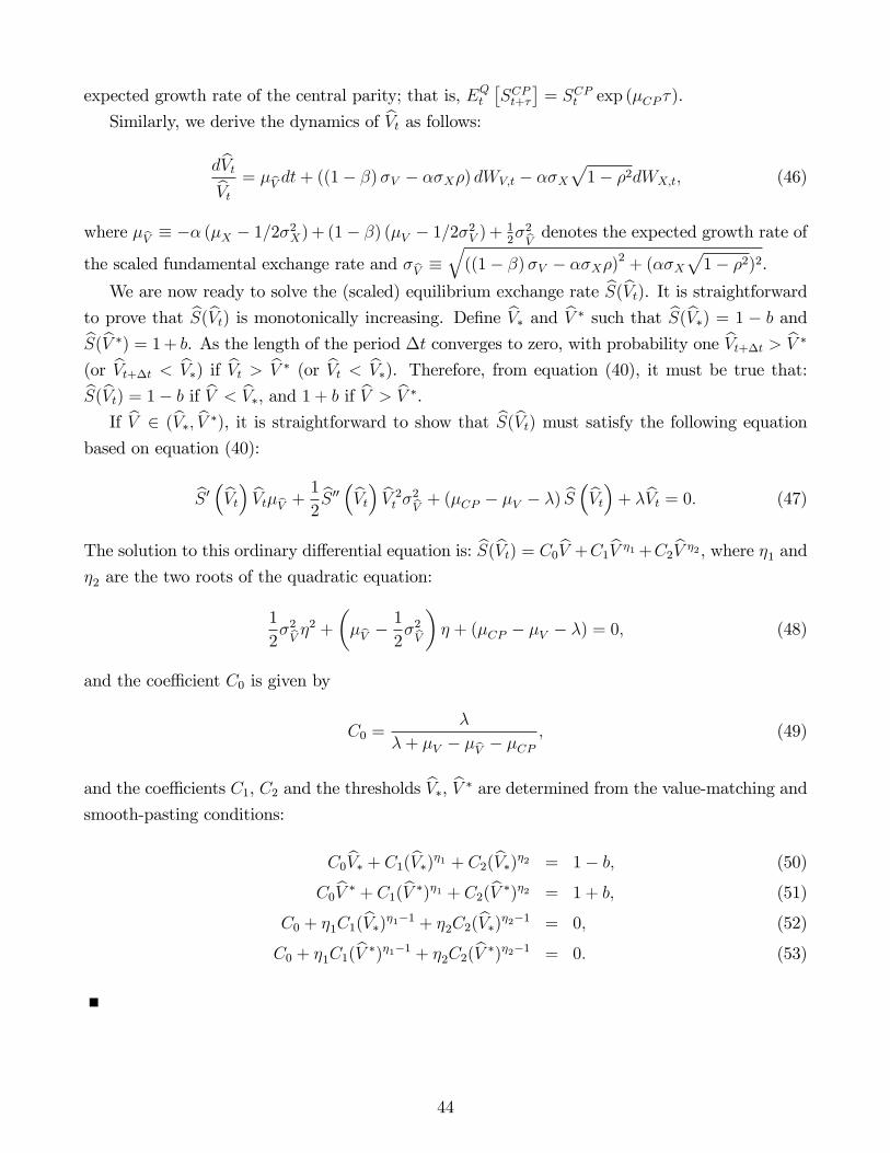
expected growth rate of the central parity; that is, EQt
[SCPt+τ
]= SCPt exp (µCP τ).
Similarly, we derive the dynamics of Vt as follows:
dVt
Vt= µV dt+ ((1− β)σV − ασXρ) dWV,t − ασX
√1− ρ2dWX,t, (46)
where µV ≡ −α (µX − 1/2σ2X) + (1− β) (µV − 1/2σ2
V ) + 12σ2Vdenotes the expected growth rate of
the scaled fundamental exchange rate and σV ≡√
((1− β)σV − ασXρ)2 + (ασX√
1− ρ2)2.
We are now ready to solve the (scaled) equilibrium exchange rate S(Vt). It is straightforward
to prove that S(Vt) is monotonically increasing. Define V∗ and V ∗ such that S(V∗) = 1 − b andS(V ∗) = 1 + b. As the length of the period ∆t converges to zero, with probability one Vt+∆t > V ∗
(or Vt+∆t < V∗) if Vt > V ∗ (or Vt < V∗). Therefore, from equation (40), it must be true that:
S(Vt) = 1− b if V < V∗, and 1 + b if V > V ∗.
If V ∈ (V∗, V∗), it is straightforward to show that S(Vt) must satisfy the following equation
based on equation (40):
S ′(Vt
)VtµV +
1
2S ′′(Vt
)V 2t σ
2V
+ (µCP − µV − λ) S(Vt
)+ λVt = 0. (47)
The solution to this ordinary differential equation is: S(Vt) = C0V +C1Vη1 +C2V
η2 , where η1 and
η2 are the two roots of the quadratic equation:
1
2σ2Vη2 +
(µV −
1
2σ2V
)η + (µCP − µV − λ) = 0, (48)
and the coeffi cient C0 is given by
C0 =λ
λ+ µV − µV − µCP, (49)
and the coeffi cients C1, C2 and the thresholds V∗, V ∗ are determined from the value-matching and
smooth-pasting conditions:
C0V∗ + C1(V∗)η1 + C2(V∗)
η2 = 1− b, (50)
C0V∗ + C1(V ∗)η1 + C2(V ∗)η2 = 1 + b, (51)
C0 + η1C1(V∗)η1−1 + η2C2(V∗)
η2−1 = 0, (52)
C0 + η1C1(V ∗)η1−1 + η2C2(V ∗)η2−1 = 0. (53)
44

Appendix B2: The Offshore CNH Market
Define Tt ≡ TtSCLt
and Ut ≡ VtSCLt
= VtSCPt
SCPtSCLt
= VtHb(S(Vt))
, where Hb
(S(Vt
))≡ H
(S(Vt
), 1; b
).
The equation for Tt can be written as
T(Ut
)=
1 + r$
1 + roffshorepEQ
t
[SCLt+1
SCLtHc
(T(Ut+1
))]+ (1− p) Ut
=1 + r$
1 + roffshorepEQ
t
[SCPt+1
SCPt
St+1
StHc
(T(Ut+1
))]+ (1− p) Ut,
where SCLt ≡ SCLt /SCPt , and Hc
(T(Ut+1
))≡ H
(T(Ut+1
), 1; c
).
We solve the model in continuous time. Denote 1 + roffshore ≡ exp (rCNH∆t). Note that Ut is
a monotonically increasing function of Vt, given by
Ut =VtSCLt
=Vt
S(Vt
) =
1
1−b Vt, if Vt < V∗Vt
C0Vt+C1Vη1t +C2V
η2t
, if Vt ∈[V∗, V
∗]
11+b
Vt, if V > V ∗
.
By the same argument as in the special case with b = 0, there exist V∗∗ and V ∗∗ such that
T(Vt
)= 1− c for Vt < V∗∗, and 1 + c for Vt > V ∗∗. To complete the derivation, we just need to
solve for T(Vt
)for Vt ∈
[V∗∗, V
∗∗]. Below we derive the ODE for T (Vt).
First, recall that
dVt
Vt= µV dt+ ((1− β)σV − ασXρ) dWV,t − ασX
√1− ρ2dWX,t ≡ µV dt+ σV dWV ,t,
where dWV ,t ≡ 1σV
[((1− β)σV − ασXρ) dWV,t − ασX
√1− ρ2dWX,t
]. By Ito’s lemma, we have
dSt =
[S ′VtµV +
1
2S ′′σ2
VV 2t
]dt+ S ′VtσV dWV ,t ≡ St
[µS + σSdWV ,t
],
where µS and σS are zero for Vt /∈[V∗, V
∗], and for Vt ∈
[V∗, V
∗], µS = − 1
St
[(µCP − µV − λ) St + λVt
]and σS = 1
StS ′V σV . Therefore,
dUt = d
(Vt
St
)= Ut
(µV dt+ σV dWV ,t
)− Ut
(µSdt+ σSdWV ,t
)+ Utσ
2Sdt− UtσV σSdt
= Ut
[(µV − µS + σS
(σS − σV
))dt−
(σS − σV
)dWV ,t
]≡ Ut
(µUdt+ σUdWV ,t
).
45

Next, we derive the dynamics for SCLt = SCPt St. Because
dSCPtSCPt
≡ µCPdt+ (αρσX + βσV ) dWV,t + α√
1− ρ2σXdWX,t
dS
S= µSdt+
σSσV
[((1− β)σV − ασXρ) dWV,t − ασX
√1− ρ2dWX,t
]we have
d(SCPt S
)SCPt S
= µCPdt+ (αρσX + βσV ) dWV,t + α√
1− ρ2σXdWX,t
+µSdt+ σS1
σV
[((1− β)σV − ασXρ) dWV,t − ασX
√1− ρ2dWX,t
]+σS
1
σV
[(αρσX + βσV ) ((1− β)σV − ασXρ)− σXα2
(1− ρ2
)]dt
≡ µCLdt+[(αρσX + βσV ) +
(σS/σV
)((1− β)σV − ασXρ)
]dWV,t
+(1− σS/σV
)α√
1− ρ2σXdWX,t,
where µCL ≡ µCP + µS +σS
σV
[(αρσX + βσV ) ((1− β)σV − ασXρ)− σXα2 (1− ρ2)].
Lastly, in continuous time, equation (17) implies the following ODE for T(U)as a function
of U :
0 = T ′(U)UµU +
1
2T ′′(U)U2σ2
U+ (rUSD − rCNH − λ+ µCL) T
(U)
+ λUt.
It is easier to solve for T(V)as a function of V instead. Using T ′
(V)
= T ′(U)U ′(V)and
T ′′(V)
= T ′′(U)U ′(V)2
+ T ′(U)U ′′(V), the above ODE can be rewritten as one for T
(V):
0 =1
2
U2σ2U
U ′(V)2 T
′′(V)
+
UµU
U ′(V) − 1
2U2σ2
U
U ′′(V)
U ′(V)3
T ′ (V )+ (rUSD − rCNH − λ+ µCL) T
(V)
+ λU(V)
≡ θ2T′′(V)
+ θ1T′(V)
+ θ0T(V)
+ λU(V), (54)
where θ0, θ1, θ2 denote the coeffi cients of T(V), T ′
(V), and T ′′
(V), respectively. The boundary
conditions are T(V∗∗
)= 1−c, T
(V ∗∗)
= 1+c, T ′(V∗∗
)= T ′
(V ∗∗)
= 0. So it is a free-boundary
problem. Because of no closed-form solution, we solve it numerically using the finite-difference
method (FDM). We provide the detail about our numerical method shortly below.
46
Numerical Method
Because of no closed-form solution for nonzero arbitraging costs, we numerically solve the free-
boundary problem in (54) with free boundaries V∗∗, V ∗∗ using the finite-difference method (FDM).
The algorithm of solving for the optimal boundaries is based on Muthuraman and Kumar (2006).
We use the following two-step procedure to solve the free-boundary problem. We begin by
choosing arbitrary boundaries V (0)∗∗ , V ∗∗(0), and denote the closed interval between these two
boundaries as Ω0 =[V
(0)∗∗ , V ∗∗(0)
]. Initially, we choose the interval large enough to embed the
optimal interval Ω∗ within it. In the next step, we use a boundary update procedure to obtain a
new interval Ω1, which is a subset of Ω0 (i.e., Ω1 ⊆ Ω0). We will repeat the procedure to get a
sequence of the intervals Ω0, Ω1, · · · until it converges to the optimal interval Ω∗ associated with
the optimal boundaries V∗∗, V ∗∗.
• In step 1, given Ωm =[V
(m)∗∗ , V ∗∗(m)
], we solve the ODE in (54) with the boundary conditions
that T(V
(m)∗∗
)= 1− c and T
(V ∗∗(m)
)= 1 + c. It can be easily solved using a FDM scheme.
Specifically, we construct a equally spaced gridV
(m)n
Nn=1
within the interval Ωm such that
V(m)
1 = V(m)∗∗ and V (m)
N = V ∗∗(m). Let ∆V denote the distance between two consecutive grid
points. To simplify notation, we denote T(V
(m)n
)simply by T (m)
n . For n ∈ 2, · · · , N − 1,
we use FDM to evaluate the derivatives of T(V)at the grid point V (m)
n :
T ′(Vn
)=T(Vn+1
)− T
(Vn
)∆V
=Tn+1 − Tn
∆Vand T ′′
(Vn
)=Tn+1 − 2Tn + Tn−1
∆V 2.
Substituting the above expressions into the ODE (54) and manipulating it, we obtain
UnT(m)n+1 +MnT
(m)n +DnT
(m)n−1 = −λU
(V (m)n
),
where Un ≡ θ1
∆V+ θ2
∆V 2, Mn ≡ − θ1
∆V− 2θ2
∆V 2+ θ0, and Dn ≡ θ2
∆V 2. The value of the function
T(V)at the grid can then be solved by the linear system below:
1
D2 M2 U2
. . .
Dn Mn Un. . .
DN−1 MN−1 UN−1
1
T(m)1
T(m)2...
T(m)n
...
T(m)N−1
T(m)N
=
1− c−λU
(V
(m)2
)...
−λU(V
(m)n
)...
−λU(V
(m)N−1
)1 + c
.
47

• In step 2, we update the boundaries from Ωm to Ωm+1. Specifically, given the solutionT
(m)n
Nn=1
from the first step, we choose the updated boundary V (m+1)∗∗ (or V ∗∗(m+1)) as
the grid point at which the function T (m) achieves its minimum (or maximum). Note that
upon convergence to the optimal boundaries V∗∗ and V ∗∗, the first derivatives are both zero,
satisfying the additional boundary conditions: T ′(V∗∗
)= T ′
(V ∗∗)
= 0. As argued in
Muthuraman and Kumar (2006), the boundary update procedure in this step guarantees
that the generated sequence of Ω’s are nested.
Appendix C: International Trades and the Balance of Pay-
ments
There are totally (N + 1) countries, including the home country (indexed by N), the numeraire
country (indexed by 0), and countries in the rest of the world or ROW (indexed by 1 through
N − 1). In the context of this paper, the home country refers to China and the numeraire country
refers to the US. We lump countries 1 through N − 1 into the rest of the world (RoW). So from
now on we focus on three countries/regions: China (home country), the US (numeraire country),
and the RoW.
Suppose China (the home country, or country N) trades with N other countries, indexed by
i ∈ 0, · · · , N − 1. Let R(i)t denote the price of currency i in dollars for i = 0, · · · , N . Note
that (i) R(0)t is always equal to unity; (ii) R(N)
t is the inverse of the central parity of the RMB
against the USD; that is, R(N)t = 1/S
CP,CNY/USDt in the previous section. Assume the price of
each country’s product is 1 in terms of its currency. Hence, country i’s product costs R(i)t dollar.
The surplus in the home country’s balance of trade in terms of dollars, TBt, is defined as
exports minus imports:
TBt ≡ R(N)t
∑N−1j=0 Dj,N
t −∑N−1
j=0 R(j)t DN,j
t ,
where Dj,Nt denotes country j’s demand for the home country’s output (i.e., export from China to
country j), and DN,jt denotes the home country’s demand for country j’s output (i.e., import to
China from country j). The loglinear approximation of the trade-balance growth is given below:
∆ log TBt ≈∑N
j=0 γ(j)t−1∆ logR
(j)t ,
where the derivation and the expressions of γ(j)t−1 in Appendix A.
Let ct ≡ logSCP,CNY/USDt denote the logarithm of the central parity SCP,CNY/USD. Note that
R(N)t = 1/S
CP,CNY/USDt and hence ∆ logR
(j)t = − (ct − ct−1). Conditional on the observations of
∆ logR(j)t
N−1
j=0, minimizing the variability in the trade-balance growth leads to a basket peg. In
48

fact,
minct
(∆ log TBt)2
= minct
(∑N−1j=1 γ
(j)t−1∆ logR
(j)t − γ
(N)t−1 (ct − ct−1)
)2
.
The solution to the above optimization problem is:
ct = ct−1 −∑N−1
j=1
(−γ(j)
t−1/γ(N)t−1
)∆ logR
(j)t . (55)
The optimal exchange rate policy that minimizes the variability in the trade-balance growth
is thus a basket peg. To see this, consider a RMB index or basket of currencies of countries
j = 0, · · · , N − 1. For currency j ∈ 1, · · · , N − 1, its weight in the basket, denoted by ωj, isgiven by
ωj = −γ(j)t−1/γ
(N)t−1, j = 1, · · · , N − 1
Under additional simplifying assumptions (see Flanders and Helpman (1979) and also the appendix
in the end of the paper), we can show that the optimal weight for currency j ∈ 0, 1, · · · , N − 1is equal to share of country j in the home country’s exports. Given that the export shares are
relatively stable, we can roughly consider the weights ωjN−1j=0 largely time invariant. The weight
for the USD in the basket ω0 = 1−∑N−1
j=1 ωj is determined as well. Note that ω0 corresponds to
ωUSD in the previous section.
With the basket composition ωjN−1j=0 , the optimal central parity in (55) can be rewritten as:
ct = ct−1 −∑N−1
j=1 ωj∆ logR(j)t .
It is straightforward to show that the above central parity is actually equal to the logarithm of
the stability pillar St corresponding to the RMB index:
Bt = CB
(R
(N)t
)ω0 ∏N−1j=1
(R
(N)t /R
(j)t
)ωj≡ χR
(N)t X1−ω0
t ,
where Xt ≡ CX∏N−1
j=1
(R
(j)t
)− ωi1−ω0 and χ ≡ CB/C
1−ω0X are defined in the same way as in the
previous section.
Let st ≡ logSt denote the logarithm of the stability pillar St, then it is given by
st = ct−1 −∑N−1
j=1 ωj∆ logR(j)t = ct−1 + (1− ω0) ∆ logXt
≡ ct−1 + (1− ω0) ∆xt,
where xt ≡ logXt denotes the logarithm of the index-implied USD index Xt. As a result, a basket
49

peg is optimal if the objective is only to minimize the variability in the trade-balance growth.
Appendix D: Derivation and Proofs in the Theoretical Model
Appendix D1: The central bank’s AM problem and the solution
Recall that the central bank’s AM objective function is stated in (24), repeated below
U (Yt) = minct
ξ∆x ((1− ω0) ∆xt −∆ct)2 + ξ∆e (ct − et−1)2 + ξcc
2t∆t+ EAM
t [V (Xt)] .
Here we show that the value function U (Yt) is also a quadratic function of the state vector Yt.
We decompose the matrix V in the value function V accordingly. Note that because
1
∆tEAMt [V (Xt)] = EAM
t
[X
(1)′t V (1,1)X
(1)t + 2X
(3)t V (3,1)X
(1)t + 2X
(1)′t V (1,2)X
(2)t
]+V (3,3)c2
t + 2ctV(3,2)X
(2)t +X
(2)′t V (2,2)X
(2)t + V0
= V (3,3)c2t + 2ct
[V (3,1)A(1,1)X
(1)t−1 + V (3,2)X
(2)t
]+X
(2)′t V (2,2)X
(2)t + V0
+X(1)′t−1A
(1,1)′V (1,1)A(1,1)X(1)t−1 + E
[ε
(1)′X,tV
(1,1)ε(1)X,t
]+ 2X
(1)′t−1A
(1,1)′V (1,2)X(2)t
Denote Vcc ≡ V (3,3). Note that X(1)t−1 = Y
(2)t and X
(2)t = Y
(3)t . We can rewrite the above
equation below
1
∆tEAMt [V (Xt)] = Vccc
2t + 2ct
[V (3,1)A(1,1)Y
(2)t + V (3,2)Y
(3)t
]+ Y
(3)′t V (2,2)Y
(3)t
+Y(2)′t A(1,1)′V (1,1)A(1,1)Y
(2)t + 2Y
(2)′t A(1,1)′V (1,2)Y
(3)t + E
[ε
(1)′X,tV
(1,1)ε(1)X,t
]+ V0
Solving the optimization problem in (24) is equivalent to solving the problem below:
minct
ξ∆x
∆t((1− ω0) ∆xt −∆ct)
2 +ξ∆e
∆t(ct − et−1)2 + (Vcc + ξc) c
2t + 2ct
[V (3,1)A(1,1)Y
(2)t + V (3,2)Y
(3)t
]The solution is the following generalized two-pillar policy:
ct = w1et−1 + w2 (ct−1 + (1− ω0) ∆xt) + ht−1,
where w1 ≡ ξ∆e/∆tVcc+ξc+(ξ∆e+ξ∆x)/∆t
, w2 ≡ ξ∆x/∆tVcc+ξc+(ξ∆e+ξ∆x)/∆t
, and ht−1 ≡ −V (3,1)A(1,1)Y(2)t +V (3,2)Y
(3)t
Vcc+ξc+(ξ∆e+ξ∆x)/∆t.
Denote V (3,2) = V (3,2) − ξ∆e/∆t [0, 1, 0]. After tedious algebra (see detailed derivations in the
50

online appendix), we can show that
1
∆tU (Yt)
=ξ∆x
∆t((1− ω0) ∆xt −∆ct)
2 +ξ∆e
∆t(ct − et−1)2 + (Vcc + ξc) c
2t + 2ct
[V (3,1)A(1,1)Y
(2)t + V (3,2)Y
(3)t
]+Y
(3)′t V (2,2)Y
(3)t + Y
(2)′t A(1,1)′V (1,1)A(1,1)Y
(2)t + 2Y
(2)′t A(1,1)′V (1,2)Y
(3)t + E
[ε
(1)′X,tV
(1,1)ε(1)X,t
]+ V0
= Y(1)′t U (1,1)Y
(1)t
−
[Y
(2)′t A(1,1)′V (3,1)′V (3,1)A(1,1)Y
(2)t + Y
(3)′t V (3,2)′V (3,2)Y
(3)t + 2Y
(2)′t A(1,1)′V (3,1)′V (3,2)Y
(3)t
]Vcc + ξc + (ξ∆e + ξ∆x) /∆t
+2Y(1)′t
[w2 (1− ω0)
w1 + w2
](V (3,1)A(1,1)Y
(2)t + V (3,2)Y
(3)t
)+ ξ∆e/∆t
(d2t−1 + 2ct−1dt−1
)+Y
(3)′t V (2,2)Y
(3)t + Y
(2)′t A(1,1)′V (1,1)A(1,1)Y
(2)t + 2Y
(2)′t A(1,1)′V (1,2)Y
(3)t + E
[ε
(1)′X,tV
(1,1)ε(1)X,t
]+ V0
= Y(1)′t U (1,1)Y
(1)t + 2Y
(1)′t
[w2 (1− ω0)
w1 + w2
]V (3,1)A(1,1)Y
(2)t
+2Y(1)′t
([w2 (1− ω0)
w1 + w2
]V (3,2) +
ξ∆e
∆t
[0 0 0
0 1 0
])Y
(3)t
+Y(2)′t
[A(1,1)′V (1,1)A(1,1) − A(1,1)′V (3,1)′V (3,1)A(1,1)
Vcc + ξc + (ξ∆e + ξ∆x) /∆t
]Y
(2)t
+Y(3)′t
V (2,2) − V (3,2)′V (3,2)
Vcc + ξc + (ξ∆e + ξ∆x) /∆t+ξ∆e
∆t
0 0 0
0 1 0
0 0 0
Y (3)
t
+2Y(2)′t
[A(1,1)′V (1,2) − A(1,1)′V (3,1)′V (3,2)
Vcc + ξc + (ξ∆e + ξ∆x) /∆t
]Y
(3)t + E
[ε
(1)′X,tV
(1,1)ε(1)X,t
]+ V0
≡ Y ′tUYt + U0,
where U0 ≡ E[ε
(1)′X,tV
(1,1)ε(1)X,t
]+ V0, and U =
[U (i,j)
], i, j = 1, 2, 3, and
U (1,1) =
(Vcc + ξc +
ξ∆x + ξ∆e
∆t
)[(1− ω0)2w2 (1− w2) (1− ω0)w2 (1− w1 − w2)
(1− ω0)w2 (1− w1 − w2) (w1 + w2) (1− w1 − w2)
],
U (2,2) = A(1,1)′V (1,1)A(1,1) − A(1,1)′V (3,1)′V (3,1)A(1,1)
Vcc + ξc + (ξ∆e + ξ∆x) /∆t,
U (3,3) = V (2,2) − V (3,2)′V (3,2)
Vcc + ξc + (ξ∆e + ξ∆x) /∆t+ξ∆e
∆t
0 0 0
0 1 0
0 0 0
,
51

and
U (1,2) =
[w2 (1− ω0)
w1 + w2
]V (3,1)A(1,1),
U (1,3) =
[w2 (1− ω0)
w1 + w2
]V (3,2) +
ξ∆e
∆t
[0 0 0
0 1 0
],
U (2,3) = A(1,1)′V (1,2) − A(1,1)′V (3,1)′V (3,2)
Vcc + ξc + (ξ∆e + ξ∆x) /∆t,
and U (2,1) = U (1,2)′, U (3,1) = U (1,3)′, U (3,2) = U (2,3)′.
Appendix D2: Dynamics of the state variables
Define Zt =
[Xt
dt
]. We now derive the dynamics of the state variables. First, note that
X(1)t+1 =
[qt+1
i∗t+1
]=
[1− ρq∆t 01×5
1− ρi∗∆t 01×5
]Zt +
[0
0
]ut +
[εq,t+1
εi∗,t+1
]≡ A(1,·)Zt +B(1,·)ut + ε
(1)X,t+1.
and
X(2)t+1 =
mt
dt
it
=
mt−1 + ut
dt
α−1 (dt − (mt−1 + ut) + ct − qt)
=
0 0 1 0 0 0 0
0 0 0 0 0 0 1
−1/α 0 −1/α 0 0 1/α 1/α
Zt +
1
0
−1/α
ut≡ A(2,·)Zt +B(2,·)ut,
and
X(3)t+1 = ct+1 = w1dt + (w1 + w2) ct + w2 (1− ω0) ∆xt+1 −
V (3,1)A(1,1)X(1)t + V (3,2)X
(2)t+1
Vcc + ξc + (ξ∆e + ξ∆x) /∆t
=[− V (3,1)A(1,1)
Vcc+ξc+(ξ∆e+ξ∆x)/∆t03×1 w1 + w2 0
]Zt
−V (3,2)
(A(2,·)Zt +B(2,·)ut
)Vcc + ξc + (ξ∆e + ξ∆x) /∆t
+ w2 (1− ω0) ∆xt+1
≡ A(3,·)Zt +B(3,·)ut + w2 (1− ω0) ∆xt+1,
52

and33
Etdt+1 = (1− w1) dt + (it − i∗t ) ∆t+ (1− w1 − w2) ct − ht= (1− w1) dt +
[α−1 (dt − (mt−1 + ut) + ct − qt)− i∗t
]∆t+ (1− w1 − w2) ct − ht
= −∆t
αqt − i∗t∆t+
(∆t
α+ (1− w1 − w2)
)ct −
∆t
αmt−1 +
(1− w1 +
∆t
α
)dt −
∆t
αut
+V (3,1)A(1,1)X
(1)t + V (3,2)X
(2)t+1
Vcc + ξc + (ξ∆e + ξ∆x) /∆t
=[−∆t
α−∆t −∆t
α0 0 ∆t
α+ (1− w1 − w2) 1 + ∆t
α
]Zt +
(−∆t
α
)ut
+V (3,1)A(1,1)
Vcc + ξc + (ξ∆e + ξ∆x) /∆tX
(1)t +
V (3,2)(A(2,·)Zt +B(2,·)ut
)Vcc + ξc + (ξ∆e + ξ∆x) /∆t
≡ A(4,·)Zt +B(4,·)ut.
Therefore,
[Xt+1
Et [dt+1]
]=
X
(1)t+1
X(2)t+1
X(3)t+1
Et [dt+1]
=
A(1,·)
A(2,·)
A(3,·)
A(4,·)
Zt +
0
B(2,·)
B(3,·)
B(4,·)
ut +
ε
(1)X,t+1
0
w2 (1− w0) ∆xt+1
0
≡ AZt +But +
ε
(1)X,t+1
0
w2 (1− w0) ∆xt+1
0
(56)
33This is becauseit = α−1 (dt − (mt−1 + ut) + ct − qt)
and
dt+1 = et+1 − [w1dt + (w1 + w2) ct + w2 (1− w0) ∆xt+1 + ht]
= et+1 − et + (1− w1) dt + (1− w1 − w2) ct − w2 (1− w0) ∆xt+1 − ht
and
Et [dt+1] = Et [et+1 − et] + (1− w1) dt + (1− w1 − w2) ct − w2 (1− w0)Et [∆xt+1]− ht= (1− w1) dt + (it − i∗t ) ∆t+ (1− w1 − w2) ct − w2 (1− w0)Et [∆xt+1]− ht= (1− w1) dt + (it − i∗t ) ∆t+ (1− w1 − w2) ct − ht
where in deriving the last equality we have used the result Et [∆xt+1] = 0 under the assumption that ∆xt+1 =ε∆x,t+1.
53
Appendix D3: The central bank’s PM problem and the solution
Recall that 1∆tV (Xt) = minut ξdd
2t + ξii
2t + βEPM
t
[1
∆tU (Yt+1)
]. Note that:
ξdd2t + ξii
2t
= ξdd2t +
ξiα2
(dt −mt−1 − ut + ct − qt)2
=ξiα2q2t + 2qt
(ξiα2mt−1 −
ξiα2
(ct + dt)
)+ξiα2m2t−1 + 2mt−1
(− ξiα2
(ct + dt)
)+
(ξd +
ξiα2
)d2t
+ξiα2c2t + 2
ξiα2ctdt +
(ξu∆t
+ξiα2
)u2t + 2
[ξiα2qt +
ξiα2mt−1 −
ξiα2dt −
ξiα2ct
]ut
≡ Z ′tQZt + Z ′tWut + u′tW′Zt + u′tRut,
where Ξ ≡ ξi/α2, R = Ξ, and
Zt =
qt
i∗t
mt−1
dt−1
it−1
ct
dt
,W =
Ξ
0
Ξ
0
0
−Ξ
−Ξ
, Q =
Ξ 0 Ξ 0 0 −Ξ −Ξ
0 0 0 0 0 0 0
Ξ 0 Ξ 0 0 −Ξ −Ξ
0 0 0 0 0 0 0
0 0 0 0 0 0 0
−Ξ 0 −Ξ 0 0 Ξ Ξ
−Ξ 0 −Ξ 0 0 Ξ ξd + Ξ
.
First, note that
EPMt
[Y ′t+1UYt+1
]= U11V ar (∆x) + U22c
2t + 2 (U23ctqt + U24cti
∗t + U25ctmt + U26ctdt + U27ctit) + U33q
2t
+2 (U34qti∗t + U35qtmt + U36qtdt + U37qtit) + U44 (i∗t )
2 + 2 (U45i∗tmt + U46i
∗tdt + U47i
∗t it)
+U55m2t + 2 (U56mtdt + U57mtit) + U66d
2t + U67dtit + U77i
2t ,
where we have used the results EPMt
[1
∆tU (Yt+1)
]= EPM
t
[Y ′t+1UYt+1
]+ U0, EPM
t
[(∆xt+1)2] =
V ar (∆x) = σ2∆x∆t, and E
PMt [Yt+1] =
[0 ct qt i∗t mt dt it
]′.
54

Then after tedious algebra (see detailed derivations in the online appendix), we can show that
EPMt
[Y ′t+1UYt+1
]=
(U33 −
2
αU37 +
U77
α2
)q2t + 2qt
( (U34 − U47
α
)i∗t +
(U35 − U57+U37
α+ U77
α2
)mt−1
+(U23 − U27−U37
α− U77
α2
)ct +
(U36 − U67−U37
α− U77
α2
)dt
)
+U44 (i∗t )2 + 2i∗t
((U45 −
1
αU47
)mt−1 +
(U24 +
1
αU47
)ct +
(U46 +
1
αU47
)dt
)+
(U55 −
2
αU57 +
1
α2U77
)m2t−1 + 2mt−1
( (U25 − 1
α(U27 − U57)− 1
α2U77
)ct
+(U56 − 1
α(U67 − U57)− 1
α2U77
)dt
)
+
(U22 +
2
αU27 +
U77
α2
)c2t + 2
(U26 +
U27 + U67
α+U77
α2
)ctdt +
(U66 +
2
αU67 +
U77
α2
)d2t
+2ut
( (U35 − U57+U37
α+ U77
α2
)qt +
(U45 − U47
α
)i∗t +
(U55 − 2
αU57 + U77
α2
)mt−1
+(U25 + U57−U27
α− U77
α2
)ct +
(U56 + U57−U67
α− U77
α2
)dt
)
+
(U55 −
2
αU57 +
1
α2U77
)u2t + U11V ar (∆x)
≡ Z ′tQZt + Z ′tWut + u′tW′Zt + u′tRut + U11V ar (∆x) ,
where R = U55 − 2αU57 + 1
α2U77, and
W =
U35 − 1αU57 − 1
αU37 + 1
α2U77
U45 − 1αU47
U55 − 2αU57 + 1
α2U77
0
0
U25 + 1αU57 − 1
αU27 − 1
α2U77
U56 + 1αU57 − 1
αU67 − 1
α2U77
, Q =
Q(1,1) Q(1,2) Q(1,3)
Q(2,1) Q(2,2) Q(2,3)
Q(3,1) Q(3,2) Q(3,3)
,
and
Q(1,1) =
[U33 + α−2U77 − 2α−1U37 U34 − α−1U47
U34 − α−1U47 U44
],
Q(1,2) =
[U35 + α−2U77 − α−1 (U57 + U37) 0
U45 − α−1U47 0
],
Q(1,3) =
[0 U23 − α−2U77 − α−1 (U27 − U37) U36 − α−2U77 − α−1 (U67 − U37)
0 U24 + α−1U47 U46 + α−1U47
],
55

and
Q(2,2) =
[U55 + α−2U77 − 2α−1U57 0
0 0
],
Q(2,3) =
[0 U25 − α−2U77 − α−1 (U27 − U57) U56 − α−2U77 − α−1 (U67 − U57)
0 0 0
],
Q(3,3) =
0 0 0
0 U22 + α−2U77 + 2α−1U27 U26 + α−2U77 + α−1 (U27 + U67)
0 U26 + α−2U77 + α−1 (U27 + U67) U66 + α−2U77 + 2α−1U67
,and Q(2,1) = Q(1,2)′, Q(3,1) = Q(1,3)′, Q(2,3) = Q(3,2)′.
Next, we now solve the above problem of the central bank at the PM of period t. This
solution is derived as follows. First, the matrices A, Q, and B are decomposed according to the
decomposition of Zt = (Xt, dt)′:
A =
[A11 A12
A21 A22
], Q =
[Q11 Q12
Q21 Q22
], B =
[B1
B2
]
Second, given dt = DXt, from (56), we have
Et [dt+1] = A21Xt + A22dt +B2ut = Dt+1Et [Xt+1] = Dt+1 (A11Xt + A12dt +B1ut) ,
dt = (A22 −Dt+1A12)−1 [(Dt+1A11 − A21)Xt + (Dt+1B1 −B2)ut] ≡ HtXt +Gtut,
where Ht ≡ (A22 −Dt+1A12)−1 (Dt+1A11 − A21) and Gt ≡ (A22 −Dt+1A12)−1 (Dt+1B1 −B2).
Third, substitution and identification of the terms in (23) results in
1
∆tV (Xt) = X ′tVtXt + V0,t
= minut
ξdd2t + ξii
2t + ξ∆d (∆dt)
2 /∆t+ ξ∆i (∆it)2 /∆t+ ξuu
2t/∆t+ βEPM
t
[1
∆tU (Yt+1)
]= min
ut(X ′tQ
∗tXt +X ′tW
∗ut + u′tW∗′t Xt + u′tR
∗tut)
+β(X ′tQ
∗tXt +X ′tW
∗ut + u′tW∗′t Xt + u′tR
∗tut + U11V ar (∆x)
),
where Q∗t ≡ Q11 + Q12Ht + H ′tQ21 + H ′tQ22Ht, W ∗t ≡ W1 + H ′tW2 + Q12Gt + H ′tQ22Gt, R∗t ≡
R +G′tW2 +W ′2Gt +G′tQ22Gt. Similarly defined are Q∗t , U
∗t , and R
∗t .
Fourth, optimization gives the standard result that the optimal choice of ut can be expressed
as a feedback on Xt
ut = −(R∗t + βR∗t
)−1 (W ∗t + βW ∗
t
)′Xt ≡ −F ∗t Xt,
56

where F ∗t =(R∗t + βR∗t
)−1 (W ∗t + βW ∗
t
)′and Vt = Q∗t+βQ
∗t−(W ∗t + βW ∗
t
)F ∗t −F ∗′t
(W ∗t + βW ∗
t
)′+
F ∗′t
(R∗t + βR∗t
)F ∗t .
Finally,
dt = HtXt +Gtut = (Ht −GtF∗t )Xt ≡ DtXt,
where Dt = Ht −GtF∗t . Therefore, the stationary solution is given as in Proposition (2).
Appendix D4: Characterization of the Steady Equilibrium
In this appendix, we further characterize the steady equilibrium. In particular, we conjecture the
matrix V in the value function V to be zero, except its elements V22, V26 (= V62), and V66, where
Vij denotes the (i, j) element of the matrix V . In the online appendix, we verify that the matrix
V indeed takes the conjectured form.
One immediate implication of the conjecture is that
ht−1 = −V(3,1)A(1,1)Y
(2)t + V (3,2)Y
(3)t
Vcc + ξc + (ξ∆e + ξ∆x) /∆t= − V62 (1− ρi∗∆t)
Vcc + ξc + (ξ∆e + ξ∆x) /∆ti∗t−1
≡ hi∗t−1,
where h ≡ − V62(1−ρi∗∆t)Vcc+ξc+(ξ∆e+ξ∆x)/∆t
. Note that when the US interest rate is independent over time
(i.e., (1− ρi∗∆t) = 0), then h = 0.
As derived in the online appendix, we can further show that D =[0 D2 0 0 0 D6
],
F ∗ =[1 F2 1 0 0 F6
], H =
[G H2 G 0 0 H6
], G = ∆t/α
1+∆t/α−w1(1+D6), where D2 and D6
are the second and sixth elements of D, respectively, and F2, F6, H2, H6 are similarly defined.
These elements are determined endogenously together with the matrix V . After tedious algebra
(see the online appendix for detailed derivations), we can verify indeed the matrix V takes the
conjectured form.
Appendix E: Extended model with intraday government
intervention
In the extended model, the government’s AM problem of choosing central parity is the same as in
the baseline model. Under the simplifying assumptions of i.i.d. processes of qt and i∗t as well as
ξ∆e = 0, the central parity has simplified rule as follows
ct+1 = w1et + w2 (ct + (1− ω0) ∆xt+1) ,
57
where w1 = ξ∆e/∆tVcc+ξc+(ξ∆e+ξ∆x)/∆t
, w2 = ξ∆x/∆tVcc+ξc+(ξ∆e+ξ∆x)/∆t
, and Vcc ≡ V (2,2). Furthermore, the gov-
ernment’s value function from its AM optimization problem is given by U (Yt) = (Y ′tUYt + U0) ∆t
where Yt = (∆xt, ct−1)′ denotes the state variable, and
U =
(Vcc + ξc +
ξ∆e + ξ∆x
∆t
)[(1− ω0)2w2 (1− w2) (1− ω0)w2 (1− w1 − w2)
(1− ω0)w2 (1− w1 − w2) (w1 + w2) (1− w1 − w2)
].
We now turn to the government’s PM problem of choosing optimal monetary policy in (23):
V (Xt) = minut
[ξdd
2t + ξii
2t
]∆t+ βEPM
t [U (Yt+1)] .
Because ∆xt follows an i.i.d. process, EPMt [U (Yt+1)], derived below, depends on only ct, not
money supply mt:
1
∆tEPMt [U (Yt+1)]
=(Vcc + ξc) (ξ∆e/∆t+ ξ∆x/∆t)
Vcc + ξc + ξ∆e/∆t+ ξ∆x/∆tc2t +
(Vcc + ξc + ξ∆e/∆t) (ξ∆x/∆t)
Vcc + ξc + ξ∆e/∆t+ ξ∆x/∆t(1− ω0)2 V ar (∆x) + U0
≡ Z ′tQZt + Z ′tWmt +m′tW′Zt + u′tRmt + U11V ar (∆x) + U0,
where R = 0, W = 05×1, and Q = diag ([0, 0, U22, 0, 0]). As a result, the government’s problem at
the PM can be simplified as choosing the level of money supply mt directly. That is,
minmt
ξdd2t + ξii
2t
= minmt
ξdd2t +
ξiα2
(dt −mt + ct − qt)2
≡ minmt
Z ′tQZt + Z ′tWmt +m′tW′Zt +m′tRmt,
where Ξ = ξi/α2, and R = Ξ,
Xt =
qt
i∗t
ct
vt
, Zt =
qt
i∗t
ct
vt
dt
, Q =
Ξ 0 −Ξ 0 −Ξ
0 0 0 0 0
−Ξ 0 Ξ 0 Ξ
0 0 0 0 0
−Ξ 0 Ξ 0 ξd + Ξ
,W = Ξ
1
0
−1
0
−1
.
Similarly as in the baseline model, the transition equation can be written as
Xt+1 = A11Xt + A12dt +B1mt + εX,t+1,
Et [dt+1] = A21Xt + A22dt +B2mt,
58

where εX,t+1 ≡ (εq,t+1, εi∗,t+1, w2 (1− ω0) ∆xt+1, vt+1)′ and
A11 =
0
0
w1 + w2
0
, A12 =
0
0
w1
0
,A21 =
[−∆t/α −∆t 1− w1 − w2 + ∆t/α −γV art
(ρt+1
)], A22 = 1− w1 + ∆t/α,
B1 = 04×1, B2 = −∆t/α.
We can solve the model similarly as before (see Appendix B1 for detailed derivation). The
basic idea is that under discretion private agents’expectations incorporate the following restriction
in a rational expectations equilibrium: dt = DXt. The restriction together with the dynamics of
the state vector Xt and the expectation Et (dt+1) imply that in equilibrium dt = HXt + Gmt
determines the exchange rate deviation as a linear function of the state vector and money supply.
Substituting the expression for dt into the government’s objective function yields
minmt
ξdd2t + ξii
2t
= minmt
X ′tQ11Xt +X ′tQ12dt + d′tQ21Xt + d′tQ22dt
+X ′tW1mt + d′tW2mt +m′tW′1Xt +m′tW
′2dt +m′tRmt
= minmt
X ′tQ11Xt +X ′tQ12 (HXt +Gmt) + (HXt +Gmt)′Q21Xt
+ (HXt +Gmt)′Q22 (HXt +Gmt) +X ′tW1mt
+ (HXt +Gmt)′W2mt +m′tW
′1Xt +m′tW
′2 (HXt +Gmt) +m′tRmt
= minmt
X ′tQ∗Xt +X ′tW
∗mt +m′tW∗′Xt +m′tR
∗mt,
where Q∗ ≡ Q11 + Q12H + H ′Q21 + H ′Q22H, W ∗ ≡ W1 + H ′W2 + Q12G + H ′Q22G, and R∗ ≡R+G′W2 +W ′
2G+G′Q22G. Therefore, the first-order condition implies the optimal money supply
mt = − (R∗)−1W ∗′Xt ≡ −F ∗Xt with F ∗ ≡ (R∗)−1W ∗′.
Special Case with ξd = 0
We now focus on a special case with ξd = 0. We conjecture that V = diag ([0, 0, Vcc, 0]) is a 4× 4
matrix of zeros, except for the last diagonal element being Vcc > 0, and that
dt = i∗t∆t− ct + γV art(ρt+1
)vt =
[0 ∆t −1 γV art
(ρt+1
)]Xt ≡ DXt.
59

Under this conjecture, we have
H = (A22 −DA12)−1 (DA11 − A21) =1
1 + ∆t/α
[∆tα
∆t −(1 + ∆t
α
)γV art
(ρt+1
)],
G = − (A22 −DA12)−1 (DB1 −B2) =∆t/α
1 + ∆t/α.
Furthermore, we can show that R∗ = Ξ(1+∆t/α)2 , W ∗ = Ξ
(1+∆t/α)2
[1 −∆t 0 −γV art
(ρt+1
)]′,
and
Q∗ =Ξ
(1 + ∆t/α)2
1 −∆t 0 −γV art
(ρt+1
)−∆t (∆t)2 0 γV art
(ρt+1
)∆t
0 0 0 0
−γV art(ρt+1
)γV art
(ρt+1
)∆t 0
(γV art
(ρt+1
))2
.Therefore, F ∗ = − (R∗)−1W ∗′ =
[1 −∆t 0 −γV art
(ρt+1
)]. The above result thus verifies that
our conjecture for D indeed holds. We can also show that Q∗ −W ∗F ∗ − F ∗′W ∗′ + F ∗′R∗F ∗ = 0.
Next, it is also straightforward to show that R∗ = 0, W ∗ = 04×1, and Q∗ = diag ([0, 0, U22, 0]).
Therefore,
V ∗ = Q∗ + βQ∗ −(W ∗t + βW ∗
t
)F ∗t − F ∗′t
(W ∗t + βW ∗
t
)′+ F ∗′t
(R∗t + βR∗t
)F ∗t = βQ∗.
It thus follows that Vcc = βU22 = β(Vcc+ξc)(ξ∆e/∆t+ξ∆x/∆t)Vcc+ξc+ξ∆e/∆t+ξ∆x/∆t
, which has a unique positive root.
Because the excess return is given by ρt+1 = (it − i∗t ) ∆t− (et+1 − et), we have
ρt+1 − Et[ρt+1
]= − (et+1 − Et [et+1]) = −EεX,t+1,
implying that the conditional variance of the excess return ρt+1 is given by
V art(ρt+1
)= EV ar (εX,t+1)E ′ = V ar (i∗t ) (∆t)2 +
(γV art
(ρt+1
))2V ar (vt) . (57)
The above equation implies the conditional variance of the excess return V art(ρt+1
)is time
invariant. We can thus simply write it as V ar(ρt+1
).
Lastly, we can determine the spot exchange rate et as the following
et = dt + ct = i∗t∆t+ γV ar(ρt+1
)vt ≡ EXt,
where E ≡(0,∆t, 0, γV ar
(ρt+1
)). Thus V ar (et) = V ar
(ρt+1
).
60


![International Policy Coordination and RMB ... - imi.ruc.edu.cn · IMI Working Paper No. 1916 [EN] International Policy Coordination and RMB Internationalisation: Theory and Historical](https://img.pdfslide.net/doc/110x75/5fe294491b710f382d0c5037/international-policy-coordination-and-rmb-imiruceducn-imi-working-paper.jpg)