The Universal Grids and the Transverse Mercator …earth-info.nga.mil/GandG/update/coordsys/resources/NGA...The Universal Grids and the Transverse Mercator and Polar Stereographic

NGA.SIG.0012_2.0.0_UTMUPS 2014-03-25

NATIONAL GEOSPATIAL-INTELLIGENCE AGENCY

STANDARDIZATION DOCUMENT

Implementation Practice

The Universal Grids and the

Transverse Mercator and Polar

Stereographic Map Projections

2014-03-25

Version 2.0.0

OFFICE OF GEOMATICS

This page is left intentionally blank.

NATIONAL GEOSPATIAL-INTELLIGENCE AGENCY

STANDARDIZATION DOCUMENT

Implementation Practice

(Revision of DMA Technical Manual 8358.2 dated 18 September 1989)

The Universal Grids and the

Transverse Mercator and Polar

Stereographic Map Projections

March 25, 2014

NGA.SIG.0012_2.0.0_UTMUPS 2014-03-25

3

Table of Contents

Preliminaries and Ellipsoid

1. General 8

1.1 Introduction 8

1.2 Purpose and scope 8

1.3 Previous edition 8

1.4 What’s new 8

1.5 What’s old 9

1.6 Meters, radians, Pi 9

1.7 Inverse trigonometric functions 9

1.8 Sign, Floor, Round 10

2. Reference Ellipsoid 11

2.1 The reference ellipsoid 11

2.2 Longitude Λ and geodetic latitude Φ 11

2.3 Ellipsoid numerical example 12

2.4 Geocentric latitude Ψ and conformal latitude Χ 12

2.5 Illustration of Φ and Ψ 12

2.6 Given Φ, compute Ψ 13

2.7 Given Ψ, compute Φ 13

2.8 Given Φ, compute {cos Χ,sin Χ} 13

2.9 Given {cos Χ, sin Χ}, compute Φ 14

2.10 Using Ψ as a substitute for Χ 14

Transverse Mercator and UTM

3. Basic Transverse Mercator 15

3.1 Definition of transverse Mercator 15

3.2 Given Λ, Φ, compute x, y 15

3.3 Notes to the developer 16

3.4 Forward mapping: a numerical example 17

3.5 Given x, y, compute Λ, Φ 17

3.6 Inverse mapping: a numerical example 18

3.7 Coverage of the ellipsoid 18

3.8 Index ∆ 19

3.9 Computational accuracy 19

4. Transverse Mercator for other Ellipsoids 20

4.1 Everest 1956 (India) ellipsoid 20

4.2 Other "Everest" ellipsoids 20

4.3 Airy 1830 ellipsoid 20

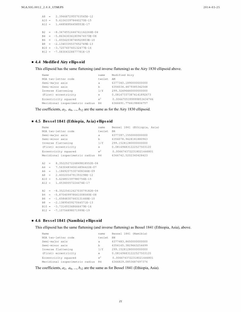
4.4 Modified Airy ellipsoid 21

4.5 Bessel 1841 (Ethiopia, Asia) ellipsoid 21

4.6 Bessel 1841 (Namibia) ellipsoid 21

4.7 Krassovsky 1940 ellipsoid 22

4.8 Helmert 1906 ellipsoid 22

4.9 Modified Fischer 1960 ellipsoid 22

4.10 WGS 72 ellipsoid 22


4.12 GRS 80 ellipsoid 23

4.13 South American 1969 ellipsoid 23

4.14 Australian National 1966 ellipsoid 24

4.15 Indonesian 1974 ellipsoid 24

4.16 International 1924 ellipsoid 24

4.17 Hough 1960 ellipsoid 25

4.18 War Office 1924 ellipsoid 25

4.19 Clarke 1866 ellipsoid 25

4.20 Clarke 1880 (IGN) ellipsoid 26



4.23 Sphere 26

NGA.SIG.0012_2.0.0_UTMUPS 2014-03-25

4

4. Transverse Mercator for other Ellipsoids 20

4.1 Everest 1956 (India) ellipsoid 20

4.2 Other "Everest" ellipsoids 20

4.3 Airy 1830 ellipsoid 20

4.4 Modified Airy ellipsoid 21

4.5 Bessel 1841 (Ethiopia, Asia) ellipsoid 21

4.6 Bessel 1841 (Namibia) ellipsoid 21

4.7 Krassovsky 1940 ellipsoid 22

4.8 Helmert 1906 ellipsoid 22

4.9 Modified Fischer 1960 ellipsoid 22



4.12 GRS 80 ellipsoid 23

4.13 South American 1969 ellipsoid 23

4.14 Australian National 1966 ellipsoid 24

4.15 Indonesian 1974 ellipsoid 24

4.16 International 1924 ellipsoid 24

4.17 Hough 1960 ellipsoid 25

4.18 War Office 1924 ellipsoid 25


4.20 Clarke 1880 (IGN) ellipsoid 26



4.23 Sphere 26

5. Transverse Mercator with Parameters 27

5.1 Preliminary general form 27

5.2 Origin 27

5.3 Given Λorigin, Φorigin, xorigin, yorigin, compute xcm, yeq 28

5.4 General form of transverse Mercator 28


5.6 History and sources 28

5.7 Old v. new 28

6. Transverse Mercator Auxiliary Functions 30

6.1 Point-scale 30

6.2 Convergence-of-meridians 30

6.3 Given Λ, Φ, compute Σ, Γ — basic case 30

6.4 Given Λ, Φ, compute Σ, Γ — general case 31

7. Universal Transverse Mercator (UTM) 32

7.1 Definition of UTM 32

7.2 Examples of computing x, y, Σ, Γ, given Λ, Φ, Z 32

7.3 Examples of computing Λ, Φ, given Z, x, y 33

7.4 Administrative rules 33

7.5 Given Λ, Φ, compute Z 34

7.6 Hierarchy of subroutines 34

Polar stereographic and UPS

8. Basic Polar Stereographic 35

8.1 Given Λ, Φ, compute x, y, Σ, Γ 35

8.2 Given x, y, compute Λ, Φ 35

9. Polar Stereographic with Parameters 37

9.1 General form (k0) 37

9.2 Origin 38

9.3 Given Λorigin, Φorigin, xorigin, yorigin, compute xpole, ypole 38

9.4 Other meanings of "Origin" 38

9.5 General form (k0, arbitrary origin) 39

9.6 Standard parallel 39

9.7 Given Φ1, compute k0 39

9.8 Given k0, compute Φ1 39

9.9 General form (Φ1, arbitrary origin) 39

9.10 Examples of conversions between Φ1 and k0 40

10. Universal Polar Stereographic (UPS) 41

10.1 Definition of UPS 41





NGA.SIG.0012_2.0.0_UTMUPS 2014-03-25

5

10. Universal Polar Stereographic (UPS) 41

10.1 Definition of UPS 41





MGRS and USNG

11. Military Grid Reference System (MGRS) 43

11.1 Character string for the UTM portion of MGRS 43

11.2 Lettering scheme “AA” 43

11.3 Lettering scheme “AL” 44

11.4 Which lettering scheme to use 44

11.5 Lettering schemes on old maps 44

11.6 Precision and digits 45

11.7 Latitude band letter 45

11.8 Latitude band letter example 45

11.9 Character string for the UPS portion of MGRS 45

11.10 Lettering scheme “UPS north” 46

11.11 Lettering scheme “UPS south” 46

11.12 Precision and digits 46

11.13 Conversion of MGRS to UTM or UPS 47

11.14 MGRS to UTM conversion example 48

11.15 Legacy tables for the lettering schemes 48

12. Topics in MGRS 51

12.1 Formal definition of MGRS 51


12.3 Rounding v. truncating 51

12.4 Point v. area 51

12.5 Latitude band letter — efficiency — northern hemisphere 52

12.6 Latitude band letter — efficiency — symmetry of tables 53

12.7 Latitude band letter — efficiency — examples 53

12.8 Latitude band letter — efficiency — southern hemisphere 54

12.9 Latitude band letter — leniency 54

12.10 Latitude band letter — leniency rule 55

12.11 MGRS–UTM hybrid 55

13. MGRS Quick-Start 56

13.1 Given Lon./Lat., compute MGRS 56

13.2 Given MGRS, compute Lon./Lat. 57

14. United States National Grid 59

14.1 Definition of USNG 59

14.2 USNG example 59

Plots and References

15. Diagrams for UTM, UPS and MGRS 61

16. References 86

NGA.SIG.0012_2.0.0_UTMUPS 2014-03-25

6

List of Symbols

Symbol Description Section(s)

a Semi-major axis of a reference ellipsoid 2.1

a2, a4... Coefficients in the series for forward transverse Mercator 3.2

A2, A4... Coefficients in the series for forward transverse Mercator 4 intro

b Semi-minor axis of a reference ellipsoid 2.1

b2, b4... Coefficients in the series for inverse transverse Mercator 3.5

B2, B4... Coefficients in the series for inverse transverse Mercator 4 intro

deg Size of one degree, in radians 1.6

f Flattening of the reference ellipsoid 2.1

f -1 Inverse flattening; reciprocal flattening 2.1

f1, f2 ... (various functions for forward mapping equations) 3.2, 6.3, 8.1

g1, g2 ... (various functions for inverse mapping equations) 3.5, 8.2

k0 Scale factor mandated for the central meridian or for the Pole 5.1, 9.1

P (an intermediate variable for some latitude conversions) 2.8

Pn (an intermediate variable for some latitude conversions) 2.9

R4 Meridional isoperimetric radius 3.2

u (an intermediate variable for basic transverse Mercator) 3.2

v (an intermediate variable for basic transverse Mercator) 3.2

w (an intermediate variable depending on ) 2.2

x Map projection plane abscissa; distance on the horizontal axis; Easting 2.1, 5.1, 8.1...

X First of three Cartesian coordinates for 3D Euclidean space 2.1

y Map projection plane ordinate; distance on the vertical axis; Northing 2.1, 5.1, 8.1...

Y Second of three Cartesian coordinates for 3D Euclidean space 2.1

Z Third of three Cartesian coordinates for 3D Euclidean space 2.1

Γ Convergence-of-meridians angle; grid declination 6.3, 8.1

e (First) eccentricity of the reference ellipsoid 2.1

Λ Longitude 2.2

Λ0 Longitude of the central meridian 5.1, 9.1

Π Pi, the ratio of a circle’s circumference to its diameter 1.6

Σ Local scale (factor) 6.3, 8.1

Φ Geodetic latitude; latitude 2.2

Χ Conformal latitude 2.4

Ψ Geocentric latitude 2.4

NGA.SIG.0012_2.0.0_UTMUPS 2014-03-25

7

1. General

� 1.1 Introduction

Earth features are commonly referenced by geographic coordinates — longitude and latitude. However, these coordi-

nates are not suitable in all situations to report positions or to calculate distances or directions. To perform these

functions conveniently, grids and grid coordinate systems have been invented. A national grid is devised by a national

authority and covers a single country (or part of it). The universal grids, Universal Transverse Mercator (UTM) and

Universal Polar Stereographic (UPS), were devised by the U.S. Department of Defense (DoD) and taken together

cover the whole Earth. The Military Grid Reference System (MGRS) is the pair, UTM and UPS, after some reformat-

ting (e.g. lettering) is applied to each.

� 1.2 Purpose and scope

This document defines the UTM, UPS and MGRS systems of coordinates and provides some information toward their

understanding and use in surveying, cartography, and geographic-information analysis.

Mainly, though, this document provides guidance to DoD and DoD contractors for the software implementation of

algorithms to convert between longitude/latitude, UTM or UPS, and MGRS coordinates. As a necessary step toward

that end, this document provides guidance for the software implementation of the transverse Mercator and polar

stereographic map projections. These map projections are endowed with parameters for general utility, of which

UTM and UPS are particular instances.

It should be noted that the previous edition, [3], had these same purposes: to define UTM and to provide the formulas

for its implementation in software. Moreover, this should be accomplished without partiality to a particular program-

ming language or software environment. Existing software, even if it were open source and government provided

(e.g. GeoTrans) and most modern and up-to-date, would not be a substitute for this document. Management of

specific DoD procurements is outside the scope of this document. Likewise also are the policies and procedures for

quality assurance of these procurements. Yet, a general recommendation can be stated: if the above conversions are

to be implemented anew, or if existing software is to be modified (for the benefits below or for other reasons), then

this document should be used to direct the development or redevelopment. This will yield the benefits explained

below under “What’s new”.

A companion to this document is NGA Standardization Document NGA.STND.0037_2.0_GRIDS, “Universal Grids

and Grid Reference Systems” [11]. DoD mapping and charting production elements should refer to it for guidance on

the proper depiction of UTM and UPS grids and MGRS labels on standard products.

Although some explanations are offered in defense of what is new, this document is not designed as a tutorial. It is

recommended to consult the map projection literature for the meaning and usefulness of grid coordinates in general

and UTM, UPS and MGRS coordinates in particular.

� 1.3 Previous edition

This document replaces technical manual DMA TM8358.2 Edition 1, “The Universal Grids: Universal Transverse

Mercator (UTM) and Universal Polar Stereographic (UPS)”, dated 18 September, 1989. Chapters 1-4 of the 1989

technical manual are superseded by this document. Chapter 5 dealt with datum transformations, which is a separate

topic and is not included in this document. Datum transformations are included in Edition 3 and Edition 4 (in prepara-

tion) of [12].

� 1.4 What’s new

The transverse Mercator map projection formulas in Section 3 are new, as explained in Subsections 5.6 and 5.7. The

new formulas provide improved efficiency and expanded coverage of the ellipsoid. Using them, the software is

shorter and simpler to write, and, by implication, less likely to have bugs.

New to this document are several sections on MGRS (Sections 11, 12, and 13). The one-dimensional tables in

Subsections 11.2 and 11.3 offer simpler logic for grid-square lettering than the traditional two-dimensional tables in

[2], but produce the same result. Some secondary matters concerning MGRS, namely non-WGS-84 lettering

(Subsection 11.4) and latitude-band-letter leniency (Subsection 12.9), have remained ambiguous (not standardized)

for years. This is corrected here for the first time in a DMA, NIMA, or NGA document. “MGRS Quick-start”

(Section 13) may be read after reading Sections 1, 2, and 3. Because it is so close to MGRS, there is a brief section

(Section 14) on the U.S. National Grid (USNG).

NGA.SIG.0012_2.0.0_UTMUPS 2014-03-25

8

New to this document are several sections on MGRS (Sections 11, 12, and 13). The one-dimensional tables in

Subsections 11.2 and 11.3 offer simpler logic for grid-square lettering than the traditional two-dimensional tables in

[2], but produce the same result. Some secondary matters concerning MGRS, namely non-WGS-84 lettering

(Subsection 11.4) and latitude-band-letter leniency (Subsection 12.9), have remained ambiguous (not standardized)

for years. This is corrected here for the first time in a DMA, NIMA, or NGA document. “MGRS Quick-start”

(Section 13) may be read after reading Sections 1, 2, and 3. Because it is so close to MGRS, there is a brief section

(Section 14) on the U.S. National Grid (USNG).

This document advocates layering of software modules, so that, for example, MGRS is a layer over UTM; UTM is a

layer over transverse Mercator with parameters; and the latter is a layer over basic transverse Mercator. Then, within

each of UTM, UPS and MGRS, some rules are described as “administrative rules” (e.g. Subsection 7.4). These are

usage oriented and not required by the theory. The recommendation is to not bundle these with the theory-required

formulas and logic, but make them a separate layer.

As a help to developers of geographic metadata formats and as a furtherance of general functionality, map projection

parameters for the transverse Mercator and polar stereographic projections are discussed in detail in Sections 5 and 9.

This yields software that is capable of both grid calculations and general cartography (map-sheet design) — a boon to

the desired consistency between these capabilities.

It is hoped that the plots and diagrams in Section 15 (all newly produced) will be useful to many. They illustrate the

principles in this document.

� 1.5 What’s old

The new formulas for transverse Mercator and UTM are consistent with the previous edition formulas where they

overlap. MGRS-needed UTM calculations, for example, are unchanged.

� 1.6 Meters, radians, pi

All lengths and distances in this document are given in meters. Readers interested in English units should be aware

that the international foot and the U.S. survey foot are slightly different. For both, a foot is 12 inches. For the U.S.

survey foot, one meter equals 39.37 (U.S. survey) inches exactly; for the international foot, one (international) inch

equals 2.54 centimeters exactly.

All angles occurring in the formulas are assumed to be in radians. One radian equals 180

Π degrees and one degree

equals Π

180 radians. When it is convenient to refer to an angle by its degree-equivalent, the notation “deg” is used as a

multiplier. Its value is deg =Π

180. For example, Λ = 23 deg =

23 Π

180. An angle occurring in a numerical table will be in

degrees, if its column heading includes the notation “(deg)”.

If the programming language does not have a built-in function for Π, the developer may establish a value for it with a

statement like pi 4 atan 1 taking the benefit of the arc-tangent function, which might be spelled “atan”.

This statement provides all the digits for Π within the chosen arithmetic precision type — single, double, or other type.

� 1.7 Inverse trigonometric functions

The (circular) trigonometric functions cosine (cos), sine (sin) and tangent (tan) take a single argument in radians.

Their inverses are defined:

arccos cos Θ = Θ, if 0 £ Θ £ Π

arcsin sin Θ = Θ, if-Π

2£ Θ £

Π

2

arctan tan Θ = Θ, if-Π

2< Θ <

Π

2

The following function is needed because some angles have values in all four quadrants and because the determina-

tion of a first-quadrant angle is numerically more robust if its cosine and sine are given than if its tangent is given. It

is called the two-argument version of arc-tangent and satisfies these identities:

(1)

arctan cos Θ, sin Θ = Θ, if - Π < Θ £ Π

arctan a x, a y = arctan x, y, if x and y are any real numbers and a > 0

arctan x, y = arctany

x, if x > 0 and y is any real number

The order of the arguments for arctan as they appear in Eq. (1.1) and in [18] might be called “x before y”. The other

convention might be called “numerator before denominator” and is the convention used in Fortran and C, where the

two-argument version of arc-tangent function is spelled “atan2”. Its relationship to arctan in this document is:

NGA.SIG.0012_2.0.0_UTMUPS 2014-03-25

9

The order of the arguments for arctan as they appear in Eq. (1.1) and in [18] might be called “x before y”. The other

convention might be called “numerator before denominator” and is the convention used in Fortran and C, where the

two-argument version of arc-tangent function is spelled “atan2”. Its relationship to arctan in this document is:

arctan x, y = atan2 y, x

Some computer languages might not have the inverse hyperbolic tangent. It is:

arctanh x =1

2Ln

1 + x

1 - x

where Ln is the natural logarithm function, that is, logarithms to the base 2.71828 ...

� 1.8 Sign, Floor, Round

Signum (sign) is the function that returns 1 if the argument is positive, 1 if the argument is negative, and 0 if the

argument is zero.

Floor is the function that returns the greatest integer less than or equal to the given number. Some examples are:

Floor1.1 = 1, Floor1 = 1, Floor-1 = -1, and Floor-1.1 = -2

Round is the function that returns the integer nearest to the given number, with half-integers rounded up. It can also

be defined:

Round x = Floor x +1

2

NGA.SIG.0012_2.0.0_UTMUPS 2014-03-25

10

2. Reference Ellipsoid

Essential for the construction of the universal grids are a reference ellipsoid and the concepts of longitude and lati-

tude, which are based upon it. These and related matters are discussed in this section.

� 2.1 The reference ellipsoid

In this document, the Earth is represented by a reference ellipsoid, defined as a surface whose points’ three-dimen-

sional Cartesian coordinates X , Y , Z satisfy the equation:

(2)X 2

a2+

Y 2

a2+

Z2

b2= 1

where a and b are constants called the semi-major and semi-minor axes, respectively. It is required that a > b. The

quantities a and b determine the flattening, f , and the eccentricity-squared, e2, as follows:

f =a - b

a= 1 -

b

a

e2=

a2 - b2

a2= 1 -

b

a

2

The flattening and the eccentricity-squared are inter-convertible as follows:

e2= f 2 - f

f =e2

1 + 1 - e2

Instead of the pair a, b as the defining parameters, the reference ellipsoid can be defined by a, f , a, f -1, a, e, or

a, e2 in which case b is given by either of these equations:

b = a 1 - f

b = a 1 - e2

The reference ellipsoid is a mathematical idealization. How it is attached to the physical Earth is outside the scope of

this document. For a treatment of this topic in general, see the geodetic literature. For its part in the establishment of

some modern terrestrial reference systems see [12] and [13].

� 2.2 Longitude Λ and geodetic latitude Φ

As stated above, a point in space lies on the reference ellipsoid if its coordinates X , Y , Z satisfy Eq. (2.2). Equiva-

lently, a point in space lies on the reference ellipsoid if its coordinates X , Y , Z can be generated by the following

formulas:

(3)

X =a

wcos Φ cos Λ

Y =a

wcos Φ sin Λ

Z =a 1 - e2

wsin Φ

where

(4)w = 1 - e2 sin2Φ

and Λ and Φ are any two real numbers. The quantity Λ, which is longitude in radians, can be restricted to any interval

of length 2 Π such as -Π < Λ £ Π. The quantity Φ, which is geodetic latitude in radians, should be restricted to the

interval -Π 2 £ Φ £ Π 2.

In this section, the term for Φ is “geodetic latitude”, to distinguish it from other quantities that are 0° at the equator

and ±90° at the Poles (see Subsection 2.4). After this section and in keeping with standard usage in geography and

cartography, geodetic latitude is shortened to “latitude”.

NGA.SIG.0012_2.0.0_UTMUPS 2014-03-25

11

In this section, the term for Φ is “geodetic latitude”, to distinguish it from other quantities that are 0° at the equator

and ±90° at the Poles (see Subsection 2.4). After this section and in keeping with standard usage in geography and

cartography, geodetic latitude is shortened to “latitude”.

� 2.3 Ellipsoid numerical example

The International ellipsoid (1924) is defined by a = 6 378 388 meters and f -1 = 297.000000. Using the formulas in

Subsection 2.1, the other parts of this ellipsoid are:

Name name International 1924

NGA two-letter code twolet IN

inverse flattening 1/f 297.000000000000000

flattening f 0.00336700336700336700

eccentricity-squared e2 0.00672267002233332200

eccentricity e 0.0819918899790297674

semi-major axis a 6378388.00000000000

semi-minor axis b 6356911.94612794613

A particular point on the International ellipsoid has longitude Λ = 23 deg =23 Π

180 and geodetic latitude Φ = 47 deg =

47 Π

180.

Using Eqs. (2.3 and 2.4), the Cartesian coordinates X , Y , Z of the particular point are:

X = 4011461.001914537

Y = 1702764.171519670

Z = 4641850.497100156

� 2.4 Geocentric latitude Ψ and conformal latitude Χ

As stated above, each point on a reference ellipsoid has a longitude Λ and geodetic latitude Φ. These quantities are

sufficient to locate the point without ambiguity. Other quantities needed in this document are the geocentric latitude

Ψ and the conformal latitude Χ, whose dependencies on Φ are given by:

(5)tan Ψ = 1 - e2 tan Φ

(6)arctanhsin Χ = arctanh sin Φ - e arctanh e sin Φ

At the Equator, Φ = Ψ = Χ = 0, and at the north Pole, Φ = Ψ = Χ = 90 deg. For the southern hemisphere, changing

Φ ® -Φ implies Ψ ® -Ψ and Χ ® - Χ. The recommended steps for converting between Φ and Χ are given in

Subsections 2.8 and 2.9.

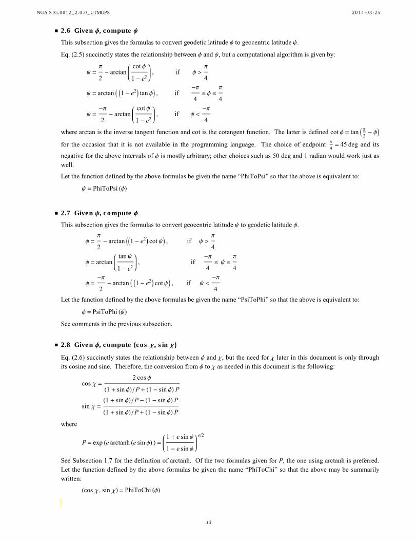
� 2.5 Illustration of Φ and Ψ

The following illustrates the concepts of reference ellipsoid, geodetic latitude Φ and geocentric latitude Ψ. The

reference ellipsoid (with greatly exaggerated flattening) is shown by its intersection with the XZ plane, i.e. the plane of

the prime meridian (Λ = 0). Point P is on the prime meridian. The line PQ is perpendicular to the ellipsoid at P. Then

Φ = ÐPQA is the geodetic latitude of P and Ψ = ÐPOA is the geocentric latitude of P.

Ψ ΦX

Z

P

O

Q

A

NGA.SIG.0012_2.0.0_UTMUPS 2014-03-25

12

� 2.6 Given Φ, compute Ψ

This subsection gives the formulas to convert geodetic latitude Φ to geocentric latitude Ψ.

Eq. (2.5) succinctly states the relationship between Φ and Ψ, but a computational algorithm is given by:

Ψ =Π

2- arctan

cot Φ

1 - e2, if Φ >

Π

4

Ψ = arctan 1 - e2 tan Φ , if-Π

4£ Φ £

Π

4

Ψ =-Π

2- arctan

cot Φ

1 - e2, if Φ <

-Π

4

where arctan is the inverse tangent function and cot is the cotangent function. The latter is defined cot Φ = tan Π

2- Φ

for the occasion that it is not available in the programming language. The choice of endpoint Π

4= 45 deg and its

negative for the above intervals of Φ is mostly arbitrary; other choices such as 50 deg and 1 radian would work just as

well.

Let the function defined by the above formulas be given the name “PhiToPsi” so that the above is equivalent to:

Ψ = PhiToPsi Φ

� 2.7 Given Ψ, compute Φ

This subsection gives the formulas to convert geocentric latitude Ψ to geodetic latitude Φ.

Φ =Π

2- arctan 1 - e2 cot Ψ , if Ψ >

Π

4

Φ = arctantan Ψ

1 - e2, if

-Π

4£ Ψ £

Π

4

Φ =-Π

2- arctan 1 - e2 cot Ψ , if Ψ <

-Π

4

Let the function defined by the above formulas be given the name “PsiToPhi” so that the above is equivalent to:

Φ = PsiToPhi Ψ

See comments in the previous subsection.

� 2.8 Given Φ, compute cos Χ, sin Χ

Eq. (2.6) succinctly states the relationship between Φ and Χ, but the need for Χ later in this document is only through

its cosine and sine. Therefore, the conversion from Φ to Χ as needed in this document is the following:

cos Χ =2 cos Φ

1 + sin Φ P + 1 - sin Φ P

sin Χ =1 + sin Φ P - 1 - sin Φ P


where

P = exp e arctanh e sin Φ =1 + e sin Φ

1 - e sin Φ

e2

See Subsection 1.7 for the definition of arctanh. Of the two formulas given for P, the one using arctanh is preferred.

Let the function defined by the above formulas be given the name “PhiToChi” so that the above may be summarily

written:

cos Χ, sin Χ = PhiToChi Φ

NGA.SIG.0012_2.0.0_UTMUPS 2014-03-25

13

� 2.9 Given cos Χ, sin Χ, compute Φ

The procedure to compute geodetic latitude Φ given the cosine and sine of the conformal latitude Χ is the following:

Φ = arctan cos Φ, sin Φ

where cos Φ is computed from sin Φ and P by:

cos Φ =1 + sin Φ P + 1 - sin Φ P

2cos Χ

where sin Φ is the limit (within desired resolution) of s1, s2, s3, ... and P is the corresponding limit of P1, P2, P3, ...

and where:

s1 = sin Χ

sn+1 =1 + sin Χ Pn

2 - 1 - sin Χ

1 + sin Χ Pn2 + 1 - sin Χ

Pn = exp e arctanh e sn =1 + e sn

1 - e sn

e2

Of the two formulas given for Pn, the one using arctanh is preferred. Let the function defined by the above formulas

be given the name “ChiToPhi” so that the above conversion is written:

Φ = ChiToPhi cos Χ, sin Χ

� 2.10 Using Ψ as a substitute for Χ

The difference between Ψ and Χ is small and Φ « Ψ conversions are faster than Φ « Χ conversions. Software develop-

ers could substitute Ψ for Χ in situations that require extreme performance and loose accuracy. Numerical investiga-

tion of the loss of accuracy would be an obligation of the developer, but here is some initial guidance:

For an ellipsoid no flatter than the ellipsoids in Section 4, the worst case occurs for the Clark 1880 ellipsoid at

Φ = ±60.1184 deg where Χ - Ψ reaches a maximum of 0.5207 arc-seconds. An error in Χ of some amount under

one second (e.g. because the formula for Ψ is used instead) propagates to an error in Φ of roughly the same amount.

NGA.SIG.0012_2.0.0_UTMUPS 2014-03-25

14

3. Basic Transverse Mercator

One of the universal grids, namely Universal Transverse Mercator (UTM), is based on the transverse Mercator map

projection. This section gives the formulas for transverse Mercator in its basic form. Later in Section 5, various

parameters such as central meridian and central scale factor will be introduced. They will enable transverse Mercator

to be offered in its commonly-used general form.

The theory of map projections and the theory of conformal mapping between surfaces are outside the scope of this

document. However, one idea from these theories is presented. The formulas for transverse Mercator will be new,

and the theoretical definition of transverse Mercator in Subsection 3.1 is appropriate as a bridge between old, e.g.

[16], and new.

In this section, any constant dependent on a reference ellipsoid will have the value pertaining to the WGS 84 ellipsoid.

Transverse Mercator for other reference ellipsoids is given in Section 4.

� 3.1 Definition of transverse Mercator

Transverse Mercator in its basic form is defined by the following requirements:

è Requirement 1: The prime meridian, i.e. the meridian at longitude Λ = 0, is portrayed on the x, y plane of the map

projection as a segment of the vertical line x = 0.

è Requirement 2: The point of intersection of the prime meridian with the Equator corresponds to the point

x, y = 0, 0 on the map projection plane.

è Requirement 3: If two points lie on the prime meridian, the distance between them on the map projection plane

will be the same as the length of meridional arc joining them on the reference ellipsoid. In other words, “distance

is preserved” (on the prime meridian).

è Requirement 4: The map projection is conformal

It is notable that the only requirement dealing with points not on the prime meridian is Requirement 4. After the

prime meridian’s points are properly placed, Requirement 4 is enough to determine the map projection’s placement of

all other points.

For readers who are familiar with transverse Mercator or who have looked ahead to Section 5, it can be stated that the

parameter choices implied by the above definition are (i) a central meridian of longitude 0 deg, (ii) a central scale

factor of 1.0000, (iii) an “Origin” point given as longitude 0 deg and latitude 0 deg, and (iv) a False Easting and a

False Northing of 0 mE and 0 mN, respectively, assigned to that origin. This is the basic form of transverse Mercator.

The formulas for transverse Mercator to follow are new (in a sense to be explained), but they adhere to the above

definition, which is not new (in effect). The above definition is implicit in the map projection literature, and both old

and new formulas are based upon it. A discussion of the relationship of this document to other authorities on trans-

verse Mercator must await the conclusion of Section 5.

� 3.2 Given Λ, Φ, compute x, y

This subsection gives the forward mapping equations for the basic form of the transverse Mercator projection. Given

the longitude Λ and latitude Φ of a point on the reference ellipsoid, the functions f1 and f2, specified below, produce

the easting x = f1Λ, Φ and northing y = f2Λ, Φ of the corresponding point on the map projection plane. They satisfy

the requirements of Subsection 3.1.

(7)

x = f1Λ, Φ= R4 u + a2 sinh2 u cos2 v + a4 sinh4 u cos4 v + ... + a12 sinh12 u cos12 v

y = f2Λ, Φ= R4 v + a2 cosh2 u sin2 v + a4 cosh4 u sin4 v + ... + a12 cosh12 u sin12 v

where cosh and sinh are the hyperbolic cosine and hyperbolic sine, respectively, and R4 and a2, a4, a6, a8, a10 and a12

are constants, and where u and v are determined by:

(8)u = arctanh cos Χ sin Λ v = arctan cos Χ cos Λ, sin Χ

NGA.SIG.0012_2.0.0_UTMUPS 2014-03-25

15

and cos Χ and sin Χ are computed according to Subsection 2.8, i.e. the function PhiToChi is applied:


For the WGS 84 ellipsoid (a = 6 378 137, f -1 = 298.257223563), the numerical values of the constants are:

(9)

R4 = 6 367 449.1458234153093 meters

a2 = 8.3773182062446983032 E 04 unitlessa4 = 7.608527773572489156 E 07 unitlessa6 = 1.19764550324249210 E 09 unitlessa8 = 2.4291706803973131 E 12 unitlessa10 = 5.711818369154105 E 15 unitlessa12 = 1.47999802705262 E 17 unitless

The quantity R4 has a name — the meridional isoperimetric radius. It is the radius of a semicircle having the same

arclength as a meridian. Its notation, R4, was chosen after seeing that notations R1, R2, R3 were adopted by [10] and

[12] for the tri-axial arithmetic-mean radius, the authalic radius, and the isovolumetric radius, respectively.

� 3.3 Notes to the developer

The previous subsection is complete for the mathematics of the forward mapping equations of the basic form of

transverse Mercator. This subsection offers additional information that might be helpful.

A series of numbers should be added from small (absolute values) to large, so as not to risk losing the full contribution

of the small numbers to the sum. Therefore, the series for x in Eq. (3.7) should begin with the last term and add each

preceding term in turn. Likewise for the series for y.

Simplicity of computer code and high performance of computer code are competing requirements for algorithm

design; it is usually not possible to achieve both. This document leans toward the former, but not exclusively, and the

following improvement for performance (speed) might be of interest to some developers. Toward the numerical

outcome required by Eq. (3.7), after cos2 v and sin2 v have been computed, the remaining multiple-angle sines and

cosines can be computed by:

(10)

cos4 v = 2 cos22 v - 1

sin4 v = 2 cos2 v sin2 vcos6 v = cos4 v cos2 v - sin4 v sin2 vsin6 v = cos4 v sin2 v + cos2 v sin4 v

and the pattern continues with:

(11)

cos8 v = 2 cos24 v - 1

sin8 v = 2 cos4 v sin4 vcos10 v = cos8 v cos2 v - sin8 v sin2 vsin10 v = cos8 v sin2 v + cos2 v sin8 vcos12 v = 2 cos26 v - 1

sin12 v = 2 cos6 v sin6 v

For the hyperbolic functions, the formulas are:

(12)

cosh4 u � 2 cosh22 u - 1

sinh4 u � 2 cosh2 u sinh2 ucosh6 u � cosh2 u cosh4 u + sinh2 u sinh4 usinh6 u � cosh4 u sinh2 u + cosh2 u sinh4 u

NGA.SIG.0012_2.0.0_UTMUPS 2014-03-25

16

and the pattern continues with:

(13)

cosh8 u � 2 cosh24 u - 1

sinh8 u � 2 cosh4 u sinh4 ucosh10 u � cosh2 u cosh8 u + sinh2 u sinh8 usinh10 u � cosh8 u sinh2 u + cosh2 u sinh8 ucosh12 u � 2 cosh26 u - 1

sinh12 u � 2 cosh6 u sinh6 u

It is in the nature of these mathematical functions that Eqs. (3.10 and 3.12) look so much alike as do Eqs. (3.11 and

3.13). A careful look at the formulas for cos6 v, and cosh6 u will reveal that they are not totally alike. The above is

correct, despite looking like there is a mistake in sign.

Eq. (3.7) as written above implies 24 calls to trigonometric functions (circular or hyperbolic). With the use of Eqs.

(3.10 through 3.13), this is reduced to merely four calls — cos2 v, sin2 v, cosh2 u and sinh2 u. The time for the

extra additions and multiplications is minuscule compared to the performance savings of fewer calls to trigonometric

functions. The extra effort to use Eqs. (3.10 through 3.13) will not suit the needs of all software developers.

It may be argued that for practical applications of transverse Mercator and UTM, Eq. (3.9) contains an excessive

number of digits. However, developers are encouraged to cut and paste the numbers as given into their code. The

computer memory locations must be filled somehow; the extra digits cause no performance degradation; and they are

not entirely inconsequential in software-testing.

The transverse Mercator projection is symmetric about the Equator and about the prime meridian. These symmetries

are contained in Eqs. (3.7, 3.8, and 3.9), which therefore apply to all four quadrants, not merely to Λ > 0 with Φ > 0.

There is no need for additional code to convert points in other quadrants. Additionally and likewise, Eqs. (3.7, 3.8,

and 3.9) get correct the (lesser known) symmetry about the meridians Λ = ±90 deg in the polar regions.

Lastly, some developers might be interested in a trade-off between accuracy and speed. Eqs. (3.10 to 3.13) were an

attempt to meet the developer’s need for speed. They do so without loss of accuracy. If that effort is insufficient, it is

admitted that fewer terms of Eq. (3.7) would be possible under a more lax accuracy requirement (Subsection 3.9) or a

more restricted reference-ellipsoid coverage requirement (Subsection 3.7), or both.

� 3.4 Forward mapping: a numerical example

Let Λ, Φ = -10 deg, 3 deg define a point on the WGS 84 ellipsoid. Then cos Χ = 0.998647785036631316 and

sin Χ = 0.0519865505821477812 by Subsection 2.8. Then u = -0.175183729646051084 and

v = 0.0528108539283539197 by Eq. (3.8). Finally, x = -1 117 373.87527102019 and y = 336 868.939627688401 by

Eq. (3.7) .

� 3.5 Given x, y, compute Λ, Φ

This subsection gives the inverse mapping equations for the basic form of the transverse Mercator projection. Given

the easting x and northing y of a point on the map projection plane, the functions g1 and g2, specified below, produce

the longitude Λ and latitude Φ of the corresponding point on the ellipsoid.

(14)Λ = g1 x, y = arctan cos v, sinh u

where u and v are computed below;

Φ = g2 x, y = ChiToPhi cos Χ, sin Χ

where the function ChiToPhi is defined in Subsection 2.9 and cos Χ is computed from u, and v as follows:

cos Χ =sinh u

cosh u sin Λ

unless sin Λ is close to zero, that is, unless:

Λ < 0.01 or Λ ± Π < 0.01 or Λ ± 2 Π < 0.01

in which case the calculation should be:

NGA.SIG.0012_2.0.0_UTMUPS 2014-03-25

17

cos Χ =sinh2 u + cos2 v

cosh u

and sin Χ is computed

sin Χ =sin v

cosh u

where u and v are computed from x and y as follows:

u =x

R4

+ b2 sinh2 x

R4

cos2 y

R4

+ b4 sinh4 x

R4

cos4 y

R4

+ ... + b12 sinh12 x

R4

cos12 y

R4

v =y

R4

+ b2 cosh2 x

R4

sin2 y

R4

+ b4 cosh4 x

R4

sin4 y

R4

+ ... + b12 cosh12 x

R4

sin12 y

R4

where R4 is defined in Subsection 3.2 and b2, b4, ... b12 are unitless constants. In the case of the WGS 84 ellipsoid,

the values are:

b2 = -8.3773216405794867707E-04

b4 = -5.905870152220365181E-08

b6 = -1.67348266534382493E-10

b8 = -2.1647981104903862E-13

b10 = -3.787930968839601E-16

b12 = -7.23676928796690E-19

Longitude at the Poles is ambiguous, i.e. not well defined. For the forward mapping equations (Section 3.2) this was

not a problem. The formulas there will correctly convert Φ = ±90 deg no matter what numerical value is used for Λ.

In this subsection, the ambiguity is a problem. The attempted computation of Λ in Eq. (3.14) will fail when the math-

library routine for arctangent encounters arctan0, 0. This will happen at a Pole, where u = 0 and v = ± Π 2, derived

from x = 0 and y = ± R4Π 2. To get around this, let the software define a constant, Λpole = 0 (suggested), and execute

Λ = Λpole if u = 0 and v = ± Π 2, and execute Eq. (3.14) otherwise.

See the notes to the developer in Subsection 3.3.

� 3.6 Inverse mapping: a numerical example

Let the reference ellipsoid be WGS 84 and let x = 400 000 and y = 7 000 000 be given. Then, in order of calculation,

u = 0.0628815005045996857, v = 1.09865807573984195, Λ = 0.137482740770994122 which in degrees is

7.87718080206913254, cos Χ = 0.458217667193810883, and sin Χ = 0.888840013428435821. Then, by the methods

of Subsection 2.9, Φ = 1.09753532362197469 which in degrees is 62.8841419100641123.

� 3.7 Coverage of the ellipsoid

For reasons beyond the scope of this document, the forward mapping equations in Subsection 3.2 are not valid for the

entire ellipsoid (i.e. the WGS 84 ellipsoid, in this section). An area surrounding each of the two points

Λ, Φ = ±90 deg, 0 deg must be omitted. Without trying to make the omitted area as small as possible, it is

possible and permitted to specify the region of validity as those points Λ, Φ which satisfy one or more of the inequali-

ties in the following list:

Λ £ 70 deg

Λ - Π £ 70 deg

Λ + Π £ 70 deg

Π

2- Φ £ 70 deg

Φ +Π

2£ 70 deg

(Recall from Subsection 1.6 that deg = Π 180 is a multiplier so that 70 deg = 7 Π 18). In words, by the above rule, any

point to be placed on a transverse Mercator map must be within 70° of longitude to the prime or anti-prime meridian

or within 70° of latitude to the North or South Pole.

NGA.SIG.0012_2.0.0_UTMUPS 2014-03-25

18

(Recall from Subsection 1.6 that deg = Π 180 is a multiplier so that 70 deg = 7 Π 18). In words, by the above rule, any

point to be placed on a transverse Mercator map must be within 70° of longitude to the prime or anti-prime meridian

or within 70° of latitude to the North or South Pole.

There is a corresponding region of validity for the inverse mapping equations. A simple, non-maximal, but adequate

choice for it is the set of all points x, y such that:

x £ 10 000 000 meters and y £ 20 000 000 meters

The above regions of validity permit all calculations of the form x, y ® Λ, Φ ® x¢, y¢, i.e. the forward mapping

equations can always be used to check an inverse-mapping-equation calculation.

� 3.8 Index ∆

As a measure of how well a point given by Λ, Φ falls within the ellipsoid coverage (Subsection 3.7) and as an index

to computational-error bounds in Subsection 3.9, the following function of Λ, Φ is defined:

∆ = Minimum Λ , Λ - Π , Λ + Π ,Π

2- Φ, Φ +

Π

2

The quantity ∆ is the minimum of the 5 quantities listed above. The ellipsoid coverage can be restated simply as

∆ £ 70 deg. In words, ∆ is the smaller of the latitude-difference to the nearest Pole and the longitude-difference to the

nearest “special” meridian (i.e. central or anti-central meridian).

� 3.9 Computational accuracy

The theoretical definition of transverse Mercator in Subsection 3.1 is the standard by which approximate formulations

such as in Subsections 3.2 and 3.5 are judged for computational accuracy. The forward mapping equations

(Subsection 3.2 using all terms) have the following computational-error bounds, depending on the index ∆:

index ∆ bound

(deg) (meters)

30 10-9

40 10-8

50 0.5´10-6

60 10-5

70 10-2

For example, if a point P has index ∆ £ 60 deg, then x - x¢2 + y - y¢2 < 10-5meters where x, y are the com-

puted coordinates and x¢, y¢ are the true coordinates of the conversion of P.

The inverse mapping equations have corresponding accuracies. In other words, the inverse mapping followed by the

true forward mapping would produce round-trip discrepancies in meters within the bounds given above.

Software developers competent in iterative numerical methods will know how to build an accurate inverse of this

document’s approximate forward mapping equations. This is discouraged, as it will not produce a more accurate

inverse mapping than the one given here.

NGA.SIG.0012_2.0.0_UTMUPS 2014-03-25

19

4. Transverse Mercator for other Ellipsoids

Section 3 was limited to one choice for the reference ellipsoid, namely the WGS 84 ellipsoid. In particular, the

constants R4, e, a2, ..., a12, b2, ... b12 all depend on the choice of the reference ellipsoid. This section provides the

values of these constants for each ellipsoid in Appendix A of [12]. A method of calculating these is found in [9].

This provision extends the formulations of transverse Mercator in Subsections 3.2 and 3.5 to these other ellipsoids.

In this section, subscripted notations are replaced by non-subscripted notations. For example, a2 is replaced by A2

and b2 is replaced by B2.

The ellipsoids are listed in order of increasing flattening (decreasing inverse flattening).

� 4.1 Everest 1956 (India) ellipsoid

Name name Everest 1956 (India)

NGA two-letter code twolet EC

Semi-major axis a 6377301.2430000000000

Semi-minor axis b 6356100.2283681013106

Inverse flattening 1/f 300.80170000000000000

(First) eccentricity e 0.081472980982652689208

Eccentricity squared e2

0.0066378466301996867553

Meridional isoperimetric radius R4 6366705.1481254190443

A2 = 8.3064943111192510534E-04

A4 = 7.480375027595025021E-07

A6 = 1.16750772278215999E-09

A8 = 2.3479972304395461E-12

A10 = 5.474212231879573E-15

A12 = 1.40642257446745E-17

B2 = -8.3064976590443772201E-04

B4 = -5.805953517555717859E-08

B6 = -1.63133251663416522E-10

B8 = -2.0923797199593389E-13

B10 = -3.630200927775259E-16

B12 = -6.87666654919219E-19

� 4.2 Other “Everest” ellipsoids

There are other ellipsoids listed in Appendix A of [12] having “Everest” in their names. They differ from the Everest

1956 (India) ellipsoid in size but not in shape. Therefore they have the same values for f , f -1, e, e2, a2, a4, ..., b12.

The value of R4 is obtained from the value of the semi-major axis, a, by multiplying by the constant

0.99833846724957337010 or by referring to the following table. (This multiplier pertains only to ellipsoids having this

shape, i.e. an inverse flattening of 300.8017).

Name code a b R4

Everest (India 1830) EA 6377276.345000 6356075.413140 6366680.291494

Everest (E. Malaysia, Brunei) EB 6377298.556000 6356097.550301 6366702.465590

Everest 1956 (India) EC 6377301.243000 6356100.228368 6366705.148125

Everest 1969 (West Malaysia) ED 6377295.664000 6356094.667915 6366699.578395

Everest 1948(W.Malaysia,Singapore) EE 6377304.063000 6356103.038993 6366707.963440

Everest (Pakistan) EF 6377309.613000 6356108.570542 6366713.504218

� 4.3 Airy 1830 ellipsoid

Name name Airy 1830

NGA two-letter code twolet AA

Semi-major axis a 6377563.3960000000000

Semi-minor axis b 6356256.9092372851202




0.0066705399999853634746


A2 = 8.3474517669594013740E-04

A4 = 7.554352936725572895E-07

A6 = 1.18487391005135489E-09

A8 = 2.3946872955703565E-12

A10 = 5.610633978440270E-15

A12 = 1.44858956458553E-17

B2 = -8.3474551646761162264E-04

B4 = -5.863630361809676570E-08

B6 = -1.65562038746920803E-10

B8 = -2.1340335537652749E-13

B10 = -3.720760760132477E-16

B12 = -7.08304328877781E-19

NGA.SIG.0012_2.0.0_UTMUPS 2014-03-25

20

Name name Airy 1830

NGA two-letter code twolet AA

Semi-major axis a 6377563.3960000000000

Semi-minor axis b 6356256.9092372851202




0.0066705399999853634746


A2 = 8.3474517669594013740E-04

A4 = 7.554352936725572895E-07

A6 = 1.18487391005135489E-09

A8 = 2.3946872955703565E-12

A10 = 5.610633978440270E-15

A12 = 1.44858956458553E-17

B2 = -8.3474551646761162264E-04

B4 = -5.863630361809676570E-08

B6 = -1.65562038746920803E-10

B8 = -2.1340335537652749E-13

B10 = -3.720760760132477E-16

B12 = -7.08304328877781E-19

� 4.4 Modified Airy ellipsoid

This ellipsoid has the same flattening (and inverse flattening) as the Airy 1830 ellipsoid above.

Name name Modified Airy

NGA two-letter code twolet AM

Semi-major axis a 6377340.1890000000000

Semi-minor axis b 6356034.4479385342568




0.0066705399999853634746


The coefficients, a2, a4, ..., b12 are the same as for the Airy 1830 ellipsoid.

� 4.5 Bessel 1841 (Ethiopia, Asia) ellipsoid

Name name Bessel 1841 (Ethiopia, Asia)

NGA two-letter code twolet BR

Semi-major axis a 6377397.1550000000000

Semi-minor axis b 6356078.9628181880963




0.0066743722318021446801


A2 = 8.3522527226849818552E-04

A4 = 7.563048340614894422E-07

A6 = 1.18692075307408346E-09

A8 = 2.4002054791393298E-12

A10 = 5.626801597980756E-15

A12 = 1.45360057224474E-17

B2 = -8.3522561262703079182E-04

B4 = -5.870409978661008580E-08

B6 = -1.65848307463131468E-10

B8 = -2.1389565927064571E-13

B10 = -3.731493368666479E-16

B12 = -7.10756898071999E-19

� 4.6 Bessel 1841 (Namibia) ellipsoid

This ellipsoid has the same flattening (and inverse flattening) as Bessel 1841 (Ethiopia, Asia), above.

Name name Bessel 1841 (Namibia)

NGA two-letter code twolet BN

Semi-major axis a 6377483.8650000000000

Semi-minor axis b 6356165.3829663254699




0.0066743722318021446801


The coefficients, a2, a4, ..., b12 are the same as for Bessel 1841 (Ethiopia, Asia).

NGA.SIG.0012_2.0.0_UTMUPS 2014-03-25

21

� 4.7 Krassovsky 1940 ellipsoid

Name name Krassovsky 1940

NGA two-letter code twolet KA

Semi-major axis a 6378245.0000000000000

Semi-minor axis b 6356863.0187730472679




0.0066934216229659432280


A2 = 8.3761175713442343106E-04

A4 = 7.606346200814720197E-07

A6 = 1.19713032035541037E-09

A8 = 2.4277772986483520E-12

A10 = 5.707722772225013E-15

A12 = 1.47872454335773E-17

B2 = -8.3761210042019176501E-04

B4 = -5.904169154078546237E-08

B6 = -1.67276212891429215E-10

B8 = -2.1635549847939549E-13

B10 = -3.785212121016612E-16

B12 = -7.23053625983667E-19

� 4.8 Helmert 1906 ellipsoid

This ellipsoid has the same flattening (and inverse flattening) as the Krassovsky 1940 ellipsoid above.

Name name Helmert 1906

NGA two-letter code twolet HE

Semi-major axis a 6378200.0000000000000

Semi-minor axis b 6356818.1696278913845




0.0066934216229659432280


The coefficients, a2, a4, ..., b12 are the same as for Krassovsky 1940.

� 4.9 Modified Fischer 1960 ellipsoid

This ellipsoid has the same flattening (and inverse flattening) as the Krassovsky 1940 ellipsoid above.

Name name Modified Fischer 1960

NGA two-letter code twolet FA

Semi-major axis a 6378155.0000000000000

Semi-minor axis b 6356773.3204827355012




0.0066934216229659432280


The coefficients, a2, a4, ..., b12 are the same as for Krassovsky 1940.

� 4.10 WGS 72 ellipsoid

Name name WGS 72

NGA two-letter code twolet WD

Semi-major axis a 6378135.0000000000000

Semi-minor axis b 6356750.5000000000000




0.0066943240336952331159


A2 = 8.3772481044362217923E-04

A4 = 7.608400388863560936E-07

A6 = 1.19761541904924067E-09

A8 = 2.4290893081322466E-12

A10 = 5.711579173743133E-15

A12 = 1.47992364667635E-17

B2 = -8.3772515386847544554E-04

B4 = -5.905770828762463028E-08

B6 = -1.67344058948464124E-10

B8 = -2.1647255130188214E-13

B10 = -3.787772179729998E-16

B12 = -7.23640523525528E-19

NGA.SIG.0012_2.0.0_UTMUPS 2014-03-25

22

Name name WGS 72

NGA two-letter code twolet WD

Semi-major axis a 6378135.0000000000000

Semi-minor axis b 6356750.5000000000000




0.0066943240336952331159


A2 = 8.3772481044362217923E-04

A4 = 7.608400388863560936E-07

A6 = 1.19761541904924067E-09

A8 = 2.4290893081322466E-12

A10 = 5.711579173743133E-15

A12 = 1.47992364667635E-17

B2 = -8.3772515386847544554E-04

B4 = -5.905770828762463028E-08

B6 = -1.67344058948464124E-10

B8 = -2.1647255130188214E-13

B10 = -3.787772179729998E-16

B12 = -7.23640523525528E-19

� 4.11 WGS 84 ellipsoid

The subsection repeats some information for the WGS 84 ellipsoid in the format of this section.

Name name WGS 84

NGA two-letter code twolet WE

Semi-major axis a 6378137.0000000000000

Semi-minor axis b 6356752.3142451794976




0.0066943799901413169961


A2 = 8.3773182062446983032E-04

A4 = 7.608527773572489156E-07

A6 = 1.19764550324249210E-09

A8 = 2.4291706803973131E-12

A10 = 5.711818369154105E-15

A12 = 1.47999802705262E-17

B2 = -8.3773216405794867707E-04

B4 = -5.905870152220365181E-08

B6 = -1.67348266534382493E-10

B8 = -2.1647981104903862E-13

B10 = -3.787930968839601E-16

B12 = -7.23676928796690E-19

� 4.12 GRS 80 ellipsoid

Name name GRS 80

NGA two-letter code twolet RF

Semi-major axis a 6378137.0000000000000

Semi-minor axis b 6356752.3141403558479




0.0066943800229007876254


A2 = 8.3773182472855134012E-04

A4 = 7.608527848149655006E-07

A6 = 1.19764552085530681E-09

A8 = 2.4291707280369697E-12

A10 = 5.711818509192422E-15

A12 = 1.47999807059922E-17

B2 = -8.3773216816203523672E-04

B4 = -5.905870210369121594E-08

B6 = -1.67348268997717031E-10

B8 = -2.1647981529928124E-13

B10 = -3.787931061803592E-16

B12 = -7.23676950110361E-19

� 4.13 South American 1969 ellipsoid

Name name South American 1969

NGA two-letter code twolet SA

Semi-major axis a 6378160.0000000000000

Semi-minor axis b 6356774.7191953059514




0.0066945418545876371598


A2 = 8.3775209887947194075E-04

A4 = 7.608896263599627157E-07

A6 = 1.19773253021831769E-09

A8 = 2.4294060763606098E-12

A10 = 5.712510331613028E-15

A12 = 1.48021320370432E-17

B2 = -8.3775244233790270051E-04

B4 = -5.906157468586898015E-08

B6 = -1.67360438158764851E-10

B8 = -2.1650081225048788E-13

B10 = -3.788390325953455E-16

B12 = -7.23782246429908E-19

NGA.SIG.0012_2.0.0_UTMUPS 2014-03-25

23

Name name South American 1969

NGA two-letter code twolet SA

Semi-major axis a 6378160.0000000000000

Semi-minor axis b 6356774.7191953059514




0.0066945418545876371598


A2 = 8.3775209887947194075E-04

A4 = 7.608896263599627157E-07

A6 = 1.19773253021831769E-09

A8 = 2.4294060763606098E-12

A10 = 5.712510331613028E-15

A12 = 1.48021320370432E-17

B2 = -8.3775244233790270051E-04

B4 = -5.906157468586898015E-08

B6 = -1.67360438158764851E-10

B8 = -2.1650081225048788E-13

B10 = -3.788390325953455E-16

B12 = -7.23782246429908E-19

� 4.14 Australian National 1966 ellipsoid

The Australian National 1966 ellipsoid is identical to the South American 1969 ellipsoid. Its NGA two-letter code is

“AN”. The numerical values of all the parameters are the same as those for South American 1969.

� 4.15 Indonesian 1974 ellipsoid

Name name Indonesian 1974

NGA two-letter code twolet ID

Semi-major axis a 6378160.0000000000000

Semi-minor axis b 6356774.5040855398378




0.0066946090804090967678


A2 = 8.3776052087969078729E-04

A4 = 7.609049308144604484E-07

A6 = 1.19776867565343872E-09

A8 = 2.4295038464530901E-12

A10 = 5.712797738386076E-15

A12 = 1.48030257891140E-17

B2 = -8.3776086434848497443E-04

B4 = -5.906276799395007586E-08

B6 = -1.67365493472742884E-10

B8 = -2.1650953495573773E-13

B10 = -3.788581120060625E-16

B12 = -7.23825990889693E-19

� 4.16 International 1924 ellipsoid

Name name International 1924

NGA two-letter code twolet IN

Semi-major axis a 6378388.0000000000000

Semi-minor axis b 6356911.9461279461279




0.0067226700223333219966


A2 = 8.4127599100356448089E-04

A4 = 7.673066923431950296E-07

A6 = 1.21291995794281190E-09

A8 = 2.4705731165688123E-12

A10 = 5.833780550286833E-15

A12 = 1.51800420867708E-17

B2 = -8.4127633881644851945E-04

B4 = -5.956193574768780571E-08

B6 = -1.69484573979154433E-10

B8 = -2.2017363465021880E-13

B10 = -3.868896221495780E-16

B12 = -7.42279219864412E-19

NGA.SIG.0012_2.0.0_UTMUPS 2014-03-25

24

� 4.17 Hough 1960 ellipsoid

This ellipsoid has the same flattening (and inverse flattening) as the International 1924 ellipsoid.

Name name Hough 1960

NGA two-letter code twolet HO

Semi-major axis a 6378270.0000000000000

Semi-minor axis b 6356794.3434343434343




0.0067226700223333219966


The coefficients, a2, a4, ..., b12 are the same as for International 1924.

� 4.18 War Office 1924 ellipsoid

Name name War Office 1924

NGA two-letter code twolet WO

Semi-major axis a 6378300.5800000000000

Semi-minor axis b 6356752.2672297297297




0.0067453433162892622352


A2 = 8.4411652150600103279E-04

A4 = 7.724989750172583427E-07

A6 = 1.22525529789972041E-09

A8 = 2.5041361775549209E-12

A10 = 5.933026083631383E-15

A12 = 1.54904908794521E-17

B2 = -8.4411687285559594196E-04

B4 = -5.996681687064322548E-08

B6 = -1.71209836918814857E-10

B8 = -2.2316811233502163E-13

B10 = -3.934782433323038E-16

B12 = -7.57474665717687E-19

� 4.19 Clarke 1866 ellipsoid

Name name Clarke 1866

NGA two-letter code twolet CC

Semi-major axis a 6378206.4000000000000

Semi-minor axis b 6356583.8000000000000




0.0067686579972910991438


A2 = 8.4703742793654652315E-04

A4 = 7.778564517658115212E-07

A6 = 1.23802665917879731E-09

A8 = 2.5390045684252928E-12

A10 = 6.036484469753319E-15

A12 = 1.58152259295850E-17

B2 = -8.4703778294785813001E-04

B4 = -6.038459874600183555E-08

B6 = -1.72996106059227725E-10

B8 = -2.2627911073545072E-13

B10 = -4.003466873888566E-16

B12 = -7.73369749524777E-19

NGA.SIG.0012_2.0.0_UTMUPS 2014-03-25

25

� 4.20 Clarke 1880 (IGN) ellipsoid

Name name Clarke 1880 (IGN)

NGA two-letter code twolet CG

Semi-major axis a 6378249.2000000000000

Semi-minor axis b 6356514.9999634416278




0.0068034876577242657616


A2 = 8.5140099460764136776E-04

A4 = 7.858945456038187774E-07

A6 = 1.25727085106103462E-09

A8 = 2.5917718627340128E-12

A10 = 6.193726879043722E-15

A12 = 1.63109098395549E-17

B2 = -8.5140135513650084564E-04

B4 = -6.101145475063033499E-08

B6 = -1.75687742410879760E-10

B8 = -2.3098718484594067E-13

B10 = -4.107860472919190E-16

B12 = -7.97633133452512E-19

� 4.21 Clarke 1880 ellipsoid

Name name Clarke 1880

NGA two-letter code twolet CD

Semi-major axis a 6378249.1450000000000

Semi-minor axis b 6356514.8695497759528




0.0068035112828490643388


A2 = 8.5140395445291970541E-04

A4 = 7.859000119464140978E-07

A6 = 1.25728397182445579E-09

A8 = 2.5918079321459932E-12

A10 = 6.193834639108787E-15

A12 = 1.63112504092335E-17

B2 = -8.5140431498554106268E-04

B4 = -6.101188106187092184E-08

B6 = -1.75689577596504470E-10

B8 = -2.3099040312610703E-13

B10 = -4.107932016207395E-16

B12 = -7.97649804397335E-19


The statements about regions of validity in Subsection 3.7 are true also for the above ellipsoids. This is because the

ellipsoids above, listed after “WGS 84 ellipsoid” are not severely flatter than the WGS 84 ellipsoid, and because the

validity regions defined in Subsection 3.7 are more restrictive than what is theoretically possible.

� 4.23 Sphere

For a sphere of radius a, the formulas of Section 3 are applicable by setting f = e2 = e = 0 and b = R4 = a and setting

all the coefficients a2, a4, ..., b12 to zero.

NGA.SIG.0012_2.0.0_UTMUPS 2014-03-25

26

5. Transverse Mercator with Parameters

Sections 3 and 4 presented the basic form of transverse Mercator. In this section, the basic form is extended two

ways: Firstly, where those sections measured longitude from the prime meridian, this section will allow longitude to

be measured from any specified meridian (“central meridian”). Secondly, the easting-northing-pairs x, y obtained

from those sections will be subjected to a homothetic transformation in this section. (A transformation is homothetic

if it consists of a translation and/or a proportional re-sizing. Rotations and other modes of stretching/shrinking are not

allowed).

This section concludes with a review of the sources consulted in the development of this document.

� 5.1 Preliminary general form

Let f1 and f2 be the functions from Subsection 3.2 that define the forward mapping of the transverse Mercator

projection in its basic form. Let Λ0 be a constant in radians, let k0 > 0 be a unitless constant, and let xcmand yeq be

constants in meters. Then a preliminary general form of the transverse Mercator forward mapping equations is:

(15)x = k0 f1Λ - Λ0, Φ + xcm

y = k0 f2Λ - Λ0, Φ + yeq

The constants, also called parameters, have these notation, names, and units:

0 central meridian, CM radians

k0 central scale factor, central scale (unitless)

xcm central meridian easting, CM easting meters

yeq Equator northing meters

The parameter k0 controls the proportional re-sizing and the parameters xcm and yeq control the translation mentioned

above. The corresponding inverse mapping equations are:

(16)

Λ = Λ0 + g1

x - xcm

k0

,y - yeq

k0

Φ = g2

x - xcm

k0

,y - yeq

k0

where functions g1 and g2 are the inverse mapping equations of the basic form of transverse Mercator specified in

Subsection 3.5.

The quantity Λ computed according to Eq. (5.16) lies in the interval Λ0 - Π < Λ £ Λ0 + Π. To convert it to a longitude

lying in a different interval (of length 2Π), the quantity 2Π should be added or subtracted to it as necessary.

The list, Λ0, k0, xcm, yeq, is a set of unique independently-specifiable parameters.

� 5.2 Origin

The equations and parameters of Subsection 5.1 accomplish the goals stated in the Section 5 introduction, which were

to (i) specify a meridian of reference (the meridian Λ0), (ii) apply a proportional re-sizing (the factor k0) and (iii) apply

a translation (the vector xcm, yeq). We should be done. However, for convenience, an alternate method to accom-

plish the translation has been adopted. This is now explained:

A point on the reference ellipsoid is selected for special treatment. It must lie in the transverse Mercator coverage

area (i.e. lie within 70° of longitude from the central or anti-central meridian or lie within 70° of latitude from the

North or South Pole), and is called the Origin. Let its longitude and latitude be notated Λorigin and Φorigin, respectively.

On the map projection plane, the Origin is to have rectangular coordinates x, y = xorigin, yorigin. This will determine

the translation under consideration.

The above parameters have these notations, names, abbreviations, and units:

Λorigin Origin longitude radians

Φorigin Origin latitude radians

xorigin (Origin easting), False Easting, FE meters

yorigin (Origin northing), False Northing, FN meters

NGA.SIG.0012_2.0.0_UTMUPS 2014-03-25

27





(If there was an opportunity to revise the terminology, “Origin easting” and “Origin northing” would make sense.

Accepted terminology is “False Easting” and “False Northing”).

� 5.3 Given Λorigin, Φorigin, xorigin, yorigin, compute xcm, yeq

Let the reference ellipsoid and transverse Mercator parameters Λ0 and k0 be fixed. Let the parameters

Λorigin, Φorigin, xorigin, yorigin be given. To obtain values for the parameters xcm, yeq that yield the same translation,

the following applies:

(17)

xcm = xorigin - k0 f1Λorigin - Λ0, Φoriginyeq = yorigin - k0 f2Λorigin - Λ0, Φorigin

� 5.4 General form of transverse Mercator

The general form of transverse Mercator is Eqs. (5.15 and 5.16) with the further stipulations that xcm and yeq are taken

as intermediate variables computed according to Eq. (5.17) and that the list Λ0, k0, Λorigin, Φorigin, xorigin, yorigin is

adopted as the general form’s set of (non-unique) independently-specifiable parameters.

Not all authorities provide the option to allow an Origin longitude distinct from the central meridian. When the set of

parameters has only one special longitude, Λorigin = Λ0 should be assumed.


The statements in Subsection 3.7 about the regions of validity for the forward and inverse mapping equations carry

over to the general form of transverse Mercator if Λ is replaced by Λ - Λ0 and x is replaced by x - xcm k0 and y is

replaced by y - yeqk0.

� 5.6 History and sources

A history of the development of transverse Mercator is outside the scope of this document, but some aspects should be

mentioned. Transverse Mercator as defined in Subsection 3.1 and extended in Subsections 5.1 or 5.4 for parameters is

sometimes given the name Gauss-Krüger or the phrase “of Gauss-Krüger type” after its inventors C. F. Gauss and L.

Krüger. This is done to distinguish it from some historical versions (Gauss-Lambert, Gauss-Schreiber) that do not

adhere to Requirement 3 of Subsection 3.1.

The formulas in Subsections 3.2 and 3.5 are extensions of the work of Krüger (1912). Krüger carried out an expan-

sion to 4th order, i.e. obtaining coefficients a2, a4, a6, a8 to some precision, and this resulted in equations which were

accurate to within 10-6 meters for points located within 1000 km of the central meridian. The algorithms given in

Section 3 extend Krüger’s method to 6th order and are based on the work of [4], [9], and [15]. Variations of Krüger’s

algorithms are in use by the national geodetic institutes of several European countries. Recently the Oil and Gas

Producers (formerly EPSG) added some version of this method to their compendium of coordinate conversion

formulas [6]. Another reference for the basic idea of Krüger’s method is Section 5.1.6, “Gauss-Kruger projection for

a wide zone” of [1].

An international standard for spatial reference frames and their coordinates, including some map projections, is

presented in [8]. The mathematical formulas it adopted for transverse Mercator do imply and are implied by the

theoretical definition in this document (Subsection 3.1). Its choice of parameters is the same as Subsection 5.4 with

Λorigin = Λ0.

� 5.7 Old v. new

Reference [3], i.e., Edition 1 of this document, and references [16] and [17] used algorithms based on an expansion in

Λ - Λ0. The major drawback of this approach is that it has a much more restricted domain of applicability, particu-

larly at high latitudes. In contrast, the algorithms given in Subsections 3.2 and 3.5 are vast improvements. They offer

better accuracy, greater ellipsoid coverage, faster execution, simpler logic, and easier software coding.

The choice of parameters in Subsection 5.4 follows current practice except that providing Λorigin as a parameter distinct

from Λ0 is new. This is recommended for its naturalness (see Subsection 5.2) and its flexibility in specifying elec-

tronic-drafting-table coordinates, especially when the map sheet has multiple plans.

NGA.SIG.0012_2.0.0_UTMUPS 2014-03-25

28

The choice of parameters in Subsection 5.4 follows current practice except that providing Λorigin as a parameter distinct

from Λ0 is new. This is recommended for its naturalness (see Subsection 5.2) and its flexibility in specifying elec-

tronic-drafting-table coordinates, especially when the map sheet has multiple plans.

Assessments of software packages in current use at DoD are outside the scope of this document. If the transverse

Mercator routines are satisfactory with respect to accuracy, ellipsoid coverage, execution speed, and code maintainabil-

ity, they need not be replaced with the algorithms specified here.

NGA.SIG.0012_2.0.0_UTMUPS 2014-03-25

29

6. Transverse Mercator Auxiliary Functions

Every conformal map projection comes with two auxiliary functions: point-scale and convergence-of-meridians

(CoM). The formulas for these for transverse Mercator are the subject of this section. Detailed explanations of the

importance and usefulness of these functions are outside the scope of this document, but some introductory definitions

will be offered.

� 6.1 Point-scale

Loosely, point-scale is the function which tells how the map projection enlarges or reduces small distances when

transferring them from the reference ellipsoid to the map projection plane. It is location specific (it varies from point

to point); it is independent of direction (conformality is required) and it is a unitless ratio (proportionality is assumed).

Let Σ (sigma, for “s” in “scaling”) be the notation for this function so that ΣP is the value of this function at position

P. If points A and B on the reference ellipsoid are one meter apart, then on the map projection plane they will be

ΣA » ΣB meters apart.

A precise definition using the differential calculus is available in the map projection literature [1], [8], [16], or [17],

where it might be called scale, local scale, local scale function, scale distortion, or point distortion.

� 6.2 Convergence-of-meridians

Convergence-of-meridians (CoM) is the function which gives the angles of intersection between the meridians and the

map projection’s vertical lines, i.e. the lines x = constant. More precisely, it is the angle from true north to map north

at such an intersection point, where the positive sense of the rotation is clockwise. True north is tangent to the

meridian and points in the direction of increasing latitude. Map north is tangent to (and coincident with) the line

x = constant and points in the direction of increasing y coordinate. All this takes place on the map projection plane.

The symbol for CoM will be Γ (gamma, for “g” in “grid declination” and “grid convergence”, synonyms for CoM

when the map projection is one of the universal grids UTM or UPS).

� 6.3 Given Λ, Φ, compute Σ, Γ — basic case

The basic form of transverse Mercator (Section 3) is handled first. Let a be the semi-major axis and e be the eccentric-

ity of the reference ellipsoid. When it is desired to emphasize the functional dependence of point-scale Σ and CoM Γ

on longitude Λ and latitude Φ, the notations f3 and f4 will be used.

The formulas for Σ and Γ are:

Σ = f3Λ, Φ =2 R4 a w cosh u Σ1

2 + Σ22


Γ = f4Λ, Φ = arctan cos Λ, sin Χ sin Λ + arctan Σ1, Σ2

where:

Σ1 = 1 + 2 a2 cosh2 u cos2 v + 4 a4 cosh4 u cos4 v + ... + 12 a12 cosh12 u cos12 vΣ2 = 2 a2 sinh2 u sin2 v + 4 a4 sinh4 u sin4 v + ... + 12 a12 sinh12 u sin12 v

w = 1 - e2 sin2Φ

P = exp e arctanh e sin Φ =1 + e sin Φ

1 - e sin Φ

e2

and where u and v are computed by Eq. (3.8) of Subsection 3.2 and R4 and the coefficients a2, a4, ..., a12 have the

same values as in Sections 3 and 4.

Depending on their requirements, software developers should consider bundling the equations of this subsection with

those of Subsection 3.2 to obtain a single module which could be described, “Given Λ, Φ, compute x, y, Σ, Γ”.

� 6.4 Given Λ, Φ, compute Σ, Γ — general case

The general form of transverse Mercator is now considered. Let the parameters Λ0, k0, Λorigin, Φorigin, xorigin, yorigin be

given. The subset Λorigin, Φorigin, xorigin, yorigin is irrelevant to the computation of Σ and Γ. Subsection 6.3 gave the

formulas for Σ and Γ for the case that Λ0 = 0 and k0 = 1. The formulas for the general case are:

NGA.SIG.0012_2.0.0_UTMUPS 2014-03-25

30

The general form of transverse Mercator is now considered. Let the parameters Λ0, k0, Λorigin, Φorigin, xorigin, yorigin be

given. The subset Λorigin, Φorigin, xorigin, yorigin is irrelevant to the computation of Σ and Γ. Subsection 6.3 gave the

formulas for Σ and Γ for the case that Λ0 = 0 and k0 = 1. The formulas for the general case are:

Σ = k0 f3 Λ - Λ0, ΦΓ = f4 Λ - Λ0, Φ

where f3 and f4 are the functions defined in Subsection 6.3. Software developers could bundle the above with Eq.

(5.15) as part of a module, “transverse Mercator preliminary general form”.

NGA.SIG.0012_2.0.0_UTMUPS 2014-03-25

31

7. Universal Transverse Mercator (UTM)

This section gives the definition of UTM, some numerical examples of it, and the administrative rules added to it.

� 7.1 Definition of UTM

UTM is a family of 120 instances of the general form of the transverse Mercator projection. Each instance is called a

zone and is given a zone number Z between -60 and +60 excluding zero. (As a connection to other explanations, the

zone numbers can be arranged suggestively this way):

+1 +2 ... +30 +31 ... +59 +60

-1 -2 ... -30 -31 ... -59 -60

UTM zone Z is the transverse Mercator projection whose parameters Λ0, k0, Λorigin, Φorigin, xorigin, yorigin are specified:

Λ0 = -183 deg + 6 deg Z using the absolute value function applied to Zk0 = 0.9996 exactly

Λorigin = Λ0

Φorigin = 0

xorigin = 500 000 meters

yorigin = 0 if Z > 0 but yorigin = 10 000 000 meters if Z < 0

Some comments apply: East longitude is positive; west longitude is negative. For Z = ±1, the central meridian in

degrees is -183 ° + 6 °´1 = -177 °, which by the above rule may be notated 177°W. The notation “-177 °W” is

incorrect. Never use both a prefix (plus or minus sign) and a suffix (“E” or “W”). A longitude in degrees can be a

UTM central meridian if and only if it is a whole number divisible by three but not by two.

� 7.2 Examples of computing x, y , Σ, Γ, given Λ, Φ, Z

This subsection gives numerical examples of the computation of the easting x, northing y, point-scale Σ, and grid-

declination Γ, given the longitude Λ, latitude Φ, and UTM zone number Z.

The following points in the Indian Ocean are symmetrically arrayed about the Equator and 75°E, which is the central

meridian for Z = ±43. Lon., Lat., and CoM are in degrees; easting and northing are in meters, and point-scale (“pt-

scale”) is a unitless ratio. The computations pertain to the WGS 84 ellipsoid.

E.g. Lon Lat Z easting northing pt-scale CoM

--- (deg) (deg) --- (meters) (meters) --- (deg)

1 65 3 43 -616926.925721 336734.192052 1.015083 -0.528835

2 74 3 43 388870.867643 331643.938073 0.999753 -0.052341

3 75 3 43 500000.000000 331593.179548 0.999600 0.000000

4 76 3 43 611129.132357 331643.938073 0.999753 0.052341

5 85 3 43 1616926.925721 336734.192052 1.015083 0.528835

6 65 -3 43 -616926.925721 -336734.192052 1.015083 0.528835

7 74 -3 43 388870.867643 -331643.938073 0.999753 0.052341

8 75 -3 43 500000.000000 -331593.179548 0.999600 0.000000

9 76 -3 43 611129.132357 -331643.938073 0.999753 -0.052341

10 85 -3 43 1616926.925721 -336734.192052 1.015083 -0.528835

Example 1, above, devolves to the example in Subsection 3.4.

The same points are re-computed for zone Z = -43, and the only change is the northing. An offset of 10,000,000

meters has been added:



11 65 3 -43 -616926.925721 10336734.192052 1.015083 -0.528835

12 74 3 -43 388870.867643 10331643.938073 0.999753 -0.052341

13 75 3 -43 500000.000000 10331593.179548 0.999600 0.000000

14 76 3 -43 611129.132357 10331643.938073 0.999753 0.052341

15 85 3 -43 1616926.925721 10336734.192052 1.015083 0.528835

16 65 -3 -43 -616926.925721 9663265.807948 1.015083 0.528835

17 74 -3 -43 388870.867643 9668356.061927 0.999753 0.052341

18 75 -3 -43 500000.000000 9668406.820452 0.999600 0.000000

19 76 -3 -43 611129.132357 9668356.061927 0.999753 -0.052341

20 85 -3 -43 1616926.925721 9663265.807948 1.015083 -0.528835

NGA.SIG.0012_2.0.0_UTMUPS 2014-03-25

32



11 65 3 -43 -616926.925721 10336734.192052 1.015083 -0.528835

12 74 3 -43 388870.867643 10331643.938073 0.999753 -0.052341

13 75 3 -43 500000.000000 10331593.179548 0.999600 0.000000

14 76 3 -43 611129.132357 10331643.938073 0.999753 0.052341

15 85 3 -43 1616926.925721 10336734.192052 1.015083 0.528835

16 65 -3 -43 -616926.925721 9663265.807948 1.015083 0.528835

17 74 -3 -43 388870.867643 9668356.061927 0.999753 0.052341

18 75 -3 -43 500000.000000 9668406.820452 0.999600 0.000000

19 76 -3 -43 611129.132357 9668356.061927 0.999753 -0.052341

20 85 -3 -43 1616926.925721 9663265.807948 1.015083 -0.528835

The following points in the Arctic region are symmetrically arrayed about the North Pole, and about the central

meridian 75°E and its anti-meridian 105 °W = 255 °E. (The first and last points are the same):



21 -105 80 43 500000.000000 11114344.070054 0.999600 -180.000000

22 -45 80 43 -469262.805167 10560437.037836 1.011097 -120.381138

23 15 80 43 -469262.805167 9435492.848206 1.011097 -59.618862

24 75 80 43 500000.000000 8881585.815988 0.999600 0.000000

25 135 80 43 1469262.805167 9435492.848206 1.011097 59.618862

26 195 80 43 1469262.805167 10560437.037836 1.011097 120.381138

27 255 80 43 500000.000000 11114344.070054 0.999600 180.000000

� 7.3 Examples of computing Λ, Φ, given Z, x, y

This subsection gives numerical examples of the computation of the longitude and latitude, given the zone number,

easting and northing. Easting and northing are in meters; longitude and latitude are in degrees. The reference ellip-

soid is WGS 84.

E.g. Z easting northing Lon Lat

--- --- (meters) (meters) (deg) (deg)

1 43 500000 0 75.0000000000 0.0000000000

2 43 600000 0 75.8986376602 0.0000000000

3 43 1000000 0 79.4887438844 0.0000000000

4 43 500000 2000000 75.0000000000 18.0887089431

5 43 600000 2000000 75.9450469497 18.0863946381

6 43 1000000 2000000 79.7195800291 18.0310022588

7 43 500000 4000000 75.0000000000 36.1447180988

8 43 600000 4000000 76.1114780322 36.1395604499

9 43 1000000 4000000 80.5461340659 36.0161920195

10 43 500000 6000000 75.0000000000 54.1481041039

11 43 600000 6000000 76.5307012564 54.1383733178

12 43 1000000 6000000 82.6176089075 53.9061008395

13 43 500000 8000000 75.0000000000 72.0992225251

14 43 600000 8000000 77.9124923218 72.0775365270

15 43 1000000 8000000 89.2856856739 71.5657403285

16 43 500000 10000000 -105.0000000000 89.9817727747

17 43 600000 10000000 166.1657933474 89.1041886301

18 43 1000000 10000000 165.2329617955 85.5261156460

19 43 500000 15000000 -105.0000000000 45.1168391850

20 43 600000 15000000 -106.2712189672 45.1097638704

21 43 1000000 15000000 -111.3373820793 44.9406465210

22 43 500000 20000000 -105.0000000000 -0.0368235977

23 43 600000 20000000 -105.8986378445 -0.0368190381

24 43 1000000 20000000 -109.4887448015 -0.0367098873

� 7.4 Administrative rules

For standard uses at DoD, there are amendments to UTM as defined above, called administrative rules. The mathemat-

ics does not require them. The most important of these rules are:

For Z > 0, UTM zone Z is intended for the portion of the reference ellipsoid given by:

Λ0 - 3 deg £ Λ < Λ0 + 3 deg and 0 £ Φ < 84 deg

For Z < 0, UTM zone Z is intended for:

Λ0 - 3 deg £ Λ < Λ0 + 3 deg and - 80 deg £ Φ < 0

The inequalities above are strict or non-strict according to the administrative rule that a zone owns its southern and

western boundaries. In other words, points on a zone’s southern and western boundaries belong to the zone but points

on its northern and eastern boundaries do not.

The above has exceptions (more administrative rules) for parts of Norway and the Arctic. These are given in [11] and

are included in Subsection 7.5.

NGA.SIG.0012_2.0.0_UTMUPS 2014-03-25

33

Examples 2,3,4 in Subsection 7.2 comply with the administrative rules; Examples 1,5-10 do not.

Software developers should be aware that the administrative rules cannot be applied in every situation, such as when

overlapping or partly overlapping UTM grids are mandated for a map sheet. Again, see [11]. Geographic informa-

tion analysts should be aware that for analytical purposes the administrative rules can be put aside in favor of obtain-

ing continuous coordinates for a region of interest. For example, UTM zone 16 coordinates could be used for hurri-

cane Katrina damage studies even where some of the damage is west of 90°W.

� 7.5 Given Λ, Φ, compute Z

This subsection gives the procedure to determine the value of Z for which UTM zone Z contains the point Λ, Φ in

compliance with the administrative rules. At the outset, if Λ = 180 deg is given, it should be converted to

Λ = -180 deg. The inequalities -180 deg £ Λ < 180 deg and -80 deg £ Φ < 84 deg should be confirmed.

Then, in pseudo-code, the procedure is:

Z = FloorΛ + 180 deg

6 deg+ 1

if Φ < 0

Z = -Z

if Z = 31 and 56 deg £ Φ < 64 deg and Λ ³ 3 deg

Z = 32

else if Z = 32 and Φ ³ 72 deg

if Λ < 9 deg

Z = 31

else

Z = 33

else if Z = 34 and Φ ³ 72 deg

if Λ < 21 deg

Z = 33

else

Z = 35

else if Z = 36 and and Φ ³ 72 deg

if Λ < 33 deg

Z = 35

else

Z = 37

� 7.6 Hierarchy of subroutines

Software design considerations are mostly beyond the scope of this document, but the following is recommended. Let

the foregoing formulas and logic be gathered into subroutines under the following hierarchy, where each subroutine is

a client of the one below it:

è UTM with administrative rules

è UTM

è transverse Mercator general form

è transverse Mercator preliminary general form

è transverse Mercator basic form

NGA.SIG.0012_2.0.0_UTMUPS 2014-03-25

34

8. Basic Polar Stereographic

The other universal grid system is Universal Polar Stereographic (UPS) and is based on the polar stereographic

projection. This section gives the formulas for the polar stereographic in its basic form. Later in Section 9, various

parameters such as zone (north or south), central meridian and central scale factor will be introduced. They will

enable polar stereographic to be offered in its commonly-used general form.

Stereographic projections in general are outside the scope of this document. The only stereographic projection treated

herein is the polar stereographic projection.

� 8.1 Given Λ, Φ, compute x, y , Σ, Γ

The basic form of the polar stereographic projection chosen for this document is centered at the north Pole and has the

following for its forward mapping equations. Let Λ, Φ be the longitude and latitude, respectively, of a point on the

reference ellipsoid excepting the south Pole. The rectangular coordinates x, y, the point-scale Σ (Subsection 6.1)

and the convergence-of-meridians Γ (Subsection 6.2) corresponding to the given point are:

(18)

x = f1Λ, Φ =2 a sin Λ cos Χ

k90 1 + sin Χ

y = f2Λ, Φ =-2 a cos Λ cos Χ

k90 1 + sin Χ

Σ = f3Λ, Φ =2 1 - e2 sin2 Φ exp e arctanh e sin Φ

k901 + sin Φ=

2 1 + e sin Φ1+e 1 - e sin Φ1-e

k901 + sin Φ

Γ = f4Λ, Φ = Λ

where, from Subsection 2.8,


and where, from Section 2, a, e are the semi-major axis and eccentricity of the reference ellipsoid. The constant k90

depends only on the reference ellipsoid and is computed by:

(19)k90 = 1 - e2 exp e arctanh e = 1 + e1+e 1 - e1-e

Where two formulas are given, namely for Σ = f3Λ, Φ and for k90, the one using arctanh is preferred. (The notation

“k90” was chosen because its value is determined by the desire to have Σ = 1 at the north Pole for the basic form).

For readers who are familiar with polar stereographic, or who have looked ahead to Section 9, it can be stated that the

parameter choices implied by Eq. (8.18) are (i) a central meridian of longitude 0 deg, (ii) a central scale factor of

1.0000, (iii) the north Pole adopted as the “Origin” point, and (iv) a False Easting and a False Northing of 0 mE and

0 mN, respectively, assigned to that origin. This is the basic form of polar stereographic.

� 8.2 Given x, y, compute Λ, Φ

The inverse mapping equations for the basic form are:

(20)Λ = g1x, y = arctan -y, xΦ = g2x, y = ChiToPhi cos Χ, sin Χ

where the function ChiToPhi is defined in Subsection 2.9 and cos Χ and sin Χ are computed by:

cos Χ =2 r

1 + r2

sin Χ =1 - r2

1 + r2

where:

NGA.SIG.0012_2.0.0_UTMUPS 2014-03-25

35

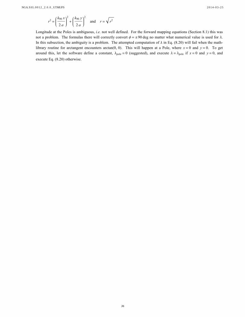
r2=

k90 x

2 a

2

+k90 y

2 a

2

and r = r2

Longitude at the Poles is ambiguous, i.e. not well defined. For the forward mapping equations (Section 8.1) this was

not a problem. The formulas there will correctly convert Φ = ±90 deg no matter what numerical value is used for Λ.

In this subsection, the ambiguity is a problem. The attempted computation of Λ in Eq. (8.20) will fail when the math-

library routine for arctangent encounters arctan0, 0. This will happen at a Pole, where x = 0 and y = 0. To get

around this, let the software define a constant, Λpole = 0 (suggested), and execute Λ = Λpole if x = 0 and y = 0, and

execute Eq. (8.20) otherwise.

NGA.SIG.0012_2.0.0_UTMUPS 2014-03-25

36

9. Polar Stereographic with Parameters

Section 8 presented the basic form of the polar stereographic projection. In this section, the basic form is extended

two ways: (i) Where Section 8 measured the longitude from the prime meridian, this section will allow longitude to

be measured from any specified meridian (“central meridian”). Then (ii), the easting-northing pairs x, y obtained

from that section will be subjected to a homothetic transformation in this section, i.e. subjected to a translation and/or

a proportional re-sizing. This follows the pattern of Section 5. (For polar stereographic but not for transverse Merca-

tor, the combination of (i) and (ii) is a similarity transformation).

� 9.1 General form (k0)

Let Z = ±1 be a flag such that Z = 1 (respectively, Z = -1) indicates the north (respectively, south) polar stereographic

projection. Let Λ0 be a constant in radians, k0 > 0 be a unitless constant, and xpole and ypole be constants in meters.

Then a general form of the polar stereographic forward mapping equations is:

(21)

For Z = +1,

x = k0 f1Λ - Λ0, Φ + xpole

y = k0 f2Λ - Λ0, Φ + ypole

Σ = k0 f3Λ - Λ0, ΦΓ = f4Λ - Λ0, Φ = Λ - Λ0

For Z = -1,

x = k0 f1Λ - Λ0, -Φ + xpole

y = -k0 f2Λ - Λ0, -Φ + ypole

Σ = k0 f3Λ - Λ0, -ΦΓ = - f4Λ - Λ0, -Φ = -Λ + Λ0

where x, y, Σ, Γ are the easting, northing, point-scale and CoM corresponding to the reference ellipsoid point at

longitude Λ and latitude Φ, and where functions f1, f2, f3, and f4 are defined in Subsection 8.1.

The constants, also called parameters, have these notations, names and units:

Λ0 central meridian, radians

longitude down from the Pole (Z = 1),

longitude up from the Pole (Z = -1).

k0 central scale, point-scale at the Pole, scale at the Pole (unitless)

xpole easting of the Pole meters

ypole northing of the Pole meters

The parameter k0 controls the proportional re-sizing and the parameters xpole and ypole control the translation men-

tioned in the introduction to this section. The corresponding inverse mapping equations are:

(22)

For Z = 1,

Λ = Λ0 + g1

x - xpole

k0

,y - ypole

k0

Φ = g2

x - xpole

k0

,y - ypole

k0

For Z = -1,

Λ = Λ0 + g1

x - xpole

k0

,y - ypole

-k0

Φ = -g2

x - xpole

k0

,y - ypole

-k0

The quantity Λ computed according to Eq. (9.22) lies in the interval Λ0 - Π < Λ £ Λ0 + Π. To convert it to a longitude

lying in a different interval (of length 2Π), the quantity 2Π should be added or subtracted to it as necessary.

The list Z, Λ0, k0, xpole, ypole is a set of unique independently-specifiable parameters.

NGA.SIG.0012_2.0.0_UTMUPS 2014-03-25

37

The list Z, Λ0, k0, xpole, ypole is a set of unique independently-specifiable parameters.

� 9.2 Origin

(This subsection is deliberately almost the same wording as Subsection 5.2 “Origin”).

The equations and parameters of Subsection 9.1 accomplish the goals stated in the Section 9 introduction, which were

to (i) specify a meridian of reference (the meridian Λ0), (ii) apply a proportional re-sizing (the factor k0) and (iii) apply

a translation (the vector xpole, ypole). More options are not a necessity. However, for convenience, an alternate

method to accomplish the translation is possible, and is now explained.

A point on the reference ellipsoid is selected for special treatment. It must lie in the ellipsoid coverage area (i.e.

outside a small region around the opposite Pole) and is called the Origin. Let its longitude and latitude be notated

Λorigin and Φorigin, respectively. On the map projection plane, the Origin is to have rectangular coordinates

x, y = xorigin, yorigin. This will determine the translation under consideration.

The above parameters have these notations, names, and units:





(If there was an opportunity to revise the terminology, “Origin easting” and “Origin northing” would make sense.

Accepted terminology is “False Easting” and “False Northing”).

� 9.3 Given Λorigin, Φorigin, xorigin, yorigin, compute xpole, ypole

Let the reference ellipsoid and polar stereographic parameters Z, Λ0, and k0 be fixed. Let the parameters

Λorigin, Φorigin, xorigin, yorigin be given. To obtain values for the parameters xpole, ypole that yield the same translation,

the following applies:

(23)

For Z = 1,

xpole = xorigin - k0 f1Λorigin - Λ0, Φoriginypole = yorigin - k0 f2Λorigin - Λ0, Φorigin

For Z = -1,

xpole = xorigin - k0 f1Λorigin - Λ0, -Φoriginypole = yorigin + k0 f2Λorigin - Λ0, -Φorigin

� 9.4 Other meanings of “Origin”

The polar stereographic projection as defined in this document should be treated as a map projection in its own right

and not as a special case of more general kinds of map projections that are called “stereographic”. Consequently, the

set of parameters has been tailored to this purpose. Moving the origin as accomplished by choosing values for

Λorigin, Φorigin, xorigin, yorigin and applying Eq. (9.23) has no affect on the shape, size, or orientation of any feature

portrayed on the map. It affects only the up/down placement of the x-axis and left/right placement of the y-axis on the

map projection plane.

By contrast, literature and software that treats the more general “stereographic” projection (not defined in this docu-

ment) might use the term “Origin” differently. Its use might include a parameter called “latitude of Origin” and

require it to be 90° to obtain the polar stereographic projection.

In this document, the concept of origin and the meaning of Λorigin, Φorigin, xorigin, yorigin are consistent between polar

stereographic and transverse Mercator. This is to the advantage of cartographers and geographic information analysts

having to try both map projections.

� 9.5 General form (k0, arbitrary origin)

An alternate general form of the polar stereographic projection is Eqs. (9.21 and 9.22) with the further stipulations that

xpole and ypole are taken as intermediate variables computed according to Eq. (9.23) and that the list

Z, Λ0, k0, Λorigin, Φorigin, xorigin, yorigin is adopted as the general form’s set of (non-unique) independently-specifiable

parameters. (The list is non-unique because more than one quadruple Λorigin, Φorigin, xorigin, yorigin will define the

same translation, i.e. the same xpole, ypole values).

NGA.SIG.0012_2.0.0_UTMUPS 2014-03-25

38

An alternate general form of the polar stereographic projection is Eqs. (9.21 and 9.22) with the further stipulations that

xpole and ypole are taken as intermediate variables computed according to Eq. (9.23) and that the list

Z, Λ0, k0, Λorigin, Φorigin, xorigin, yorigin is adopted as the general form’s set of (non-unique) independently-specifiable

parameters. (The list is non-unique because more than one quadruple Λorigin, Φorigin, xorigin, yorigin will define the

same translation, i.e. the same xpole, ypole values).

� 9.6 Standard parallel

The standard parallel, also called the latitude of unity scale, is the value of Φ in Eq. (9.21) that gives Σ = 1. It will

exist if k0 £ 1. Its notation in this document is Φ1.

� 9.7 Given Φ1, compute k0

Given the standard parallel Φ1, the formula to find the scale factor k0 at the relevant Pole is:

(24)

For Z = 1,

k0 =1

f30, Φ1=

k901 + sin Φ1

2 1 + e sin Φ11+e 1 - e sin Φ11-e

For Z = -1,

k0 =1

f30, -Φ1=

k901 - sin Φ1

2 1 - e sin Φ11+e 1 + e sin Φ11-e

� 9.8 Given k0, compute Φ1

For Z = ±1, let a value k0 < 1 for the scale factor at the Pole be given. Then the method to compute the standard

parallel Φ1 is:

Φ1 = Z arcsin s

where s is the limit (within the desired resolution) of the sequence s1, s2, s3, ... whose members are computed by:

s1 = -1 + 2 k0

sn+1 =2 k0 1 + e sn1+e 1 - e sn1-e

k90

- 1

� 9.9 General form (Φ1, arbitrary origin)

Another general form of the polar stereographic projection is Eqs. (9.21 and 9.22) with the further stipulations that

xpole, ypole, and k0 are taken as intermediate variables computed according to Eqs. (9.23 and 9.24) and that the list

Z, Λ0, Φ1, Λorigin, Φorigin, xorigin, yorigin is adopted as the general form’s set of (non-unique) independently-specifiable

parameters. Note that Φ1 replaces k0 in the list.

The adjectives “unique” and “independently-specifiable” and their negatives have been used carefully in this section

when describing lists of polar stereographic parameters. As another example, consider the list

Z, Λ0, k0, Φ1, xpole, ypole. Its parameters are all unique, but they are not all independently-specifiable because both k0

and Φ1 are listed.

NGA.SIG.0012_2.0.0_UTMUPS 2014-03-25

39

� 9.10 Examples of conversions between Φ1 and k0

The following two tables pertain to the north polar stereographic projection (Z = 1) of the WGS 84 ellipsoid

(a = 6 378 137 and f -1 = 298.257223563).

In the table at left, the values of Φ1 are exact and the values of k0 are computed to as many digits shown. In the table

at right, the values of k0 are exact, and the values of Φ1 are computed to as many digits as are shown.

1

degree

k0

unitless

75 0.017 259 384 673

60 0.067 773 950 243

45 0.147 883 853 421

30 0.251 891 492 664

15 0.372 562 837 459

0 0.501 678 277 625

15 0.630 570 160 065

30 0.750 629 794 742

45 0.853 799 593 615

60 0.933 069 071 736

75 0.982 966 757 777

80 0.992 404 648 246

81 0.993 844 677 874

82 0.995 134 351 941

83 0.996 273 262 333

84 0.997 261 048 527

85 0.998 097 397 746

86 0.998 782 045 101

87 0.999 314 773 702

88 0.999 695 414 760

89 0.999 923 847 656

90 1.000 000 000 000

k0

unitless

1

degree

0.1000 53.337 403 999 811

0.2000 37.116 011 177 617

0.3000 23.825 251 373 649

0.4000 11.763 627 302 241

0.5000 0.192 963 050 538

0.6000 11.385 608 705 462

0.7000 23.471 956 301 947

0.8000 36.808 078 424 089

0.9000 53.106 923 780 672

0.9100 55.064 894 505 323

0.9200 57.123 352 185 495

0.9300 59.302 785 064 482

0.9400 61.631 355 734 180

0.9500 64.149 649 327 832

0.9600 66.920 027 216 673

0.9700 70.047 603 511 896

0.9800 73.737 632 650 010

0.9900 78.520 890 585 055

0.9910 79.111 860 671 964

0.9920 79.736 353 686 644

0.9930 80.400 910 884 378

0.9940 81.114 517 868 594

0.9950 81.890 113 174 369

0.9960 82.747 558 146 254

0.9970 83.720 292 647 173

0.9980 84.873 530 910 724

0.9990 86.375 668 096 133

0.9991 86.561 716 515 710

0.9992 86.758 411 486 352

0.9993 86.967 824 204 285

0.9994 87.192 799 401 974

0.9995 87.437 432 634 553

0.9996 87.708 009 826 129

0.9997 88.015 112 711 542

0.9998 88.379 374 422 928

0.9999 88.854 064 538 034

1.0000 90.000 000 000 000

NGA.SIG.0012_2.0.0_UTMUPS 2014-03-25

40

10. Universal Polar Stereographic (UPS)

This section gives the definition of UPS, some numerical examples of it, and the administrative rules added to it.

� 10.1 Definition of UPS

The Universal Polar Stereographic (UPS) system is these two instances of the polar stereographic projection with

parameters. The parameters fit Eqs. (9.21 and 9.22).

North UPS is defined by:

Z = 1

Λ0 = 0 longitude down from the Polek0 = 0.994 exactlyxpole = 2 000 000

ypole = 2 000 000

South UPS is defined by:

Z = -1

Λ0 = 0 longitude up from the Polek0 = 0.994 exactlyxpole = 2 000 000

ypole = 2 000 000

� 10.2 Examples of computing x, y , Σ, Γ, given Λ, Φ, Z

The following computations pertain to the WGS 84 ellipsoid.



1 --- 90 1 2000000.000000 2000000.000000 0.994000 ---

2 -179 89 1 1998062.320046 2111009.610243 0.994076 -179

3 -90 88 1 1777930.731071 2000000.000000 0.994303 -90

4 -1 87 1 1994185.827038 1666906.254073 0.994682 -1

5 0 86 1 2000000.000000 1555731.570643 0.995212 0

6 1 85 1 2009694.068153 1444627.207468 0.995895 1

7 89 84 1 2666626.157825 1988363.997132 0.996730 89

8 90 83 1 2778095.750322 2000000.000000 0.997718 90

9 91 82 1 2889442.490749 2015525.276426 0.998860 91

10 179 81 1 2017473.190606 3001038.419357 1.000156 179

11 180 80 1 2000000.000000 3112951.136955 1.001608 180

12 0 40 1 2000000.000000 -3918313.984953 1.209619 0

13 -179 3 1 1790630.987261 13994742.706481 1.883453 -179

14 -90 2 1 -10206568.118587 2000000.000000 1.914973 -90

15 -1 1 1 1783239.204558 -10418217.653909 1.947589 -1

16 0 0 1 2000000.000000 -10637318.498257 1.981349 0

17 1 -1 1 2224408.737826 -10856367.979638 2.016305 1

18 90 -2 1 15083269.373905 2000000.000000 2.052510 90

19 179 -3 1 2232331.498720 15310262.647286 2.090020 179

20 180 -4 1 2000000.000000 15545537.944524 2.128897 180

� 10.3 Examples of computing Λ, Φ, given Z, x, y

The following computations pertain to the WGS 84 ellipsoid.



1 -1 0 0 -135.0000000000 -64.9164123332

2 -1 1000000 0 -153.4349488229 -70.0552944014

3 -1 2000000 0 -180.0000000000 -72.1263610163

4 -1 3000000 0 153.4349488229 -70.0552944014

5 -1 4000000 0 135.0000000000 -64.9164123332

6 -1 0 1000000 -116.5650511771 -70.0552944014

7 -1 1000000 1000000 -135.0000000000 -77.3120791908

8 -1 2000000 1000000 180.0000000000 -81.0106632645

9 -1 3000000 1000000 135.0000000000 -77.3120791908

10 -1 4000000 1000000 116.5650511771 -70.0552944014

11 -1 0 2000000 -90.0000000000 -72.1263610163

12 -1 1000000 2000000 -90.0000000000 -81.0106632645

13 -1 2000000 2000000 --- -90.0000000000

14 -1 3000000 2000000 90.0000000000 -81.0106632645

15 -1 4000000 2000000 90.0000000000 -72.1263610163

16 -1 0 3000000 -63.4349488229 -70.0552944014

17 -1 1000000 3000000 -45.0000000000 -77.3120791908

18 -1 2000000 3000000 0.0000000000 -81.0106632645

19 -1 3000000 3000000 45.0000000000 -77.3120791908

20 -1 4000000 3000000 63.4349488229 -70.0552944014

21 -1 0 4000000 -45.0000000000 -64.9164123332

22 -1 1000000 4000000 -26.5650511771 -70.0552944014

23 -1 2000000 4000000 0.0000000000 -72.1263610163

24 -1 3000000 4000000 26.5650511771 -70.0552944014

25 -1 4000000 4000000 45.0000000000 -64.9164123332

NGA.SIG.0012_2.0.0_UTMUPS 2014-03-25

41



1 -1 0 0 -135.0000000000 -64.9164123332

2 -1 1000000 0 -153.4349488229 -70.0552944014

3 -1 2000000 0 -180.0000000000 -72.1263610163

4 -1 3000000 0 153.4349488229 -70.0552944014

5 -1 4000000 0 135.0000000000 -64.9164123332

6 -1 0 1000000 -116.5650511771 -70.0552944014

7 -1 1000000 1000000 -135.0000000000 -77.3120791908

8 -1 2000000 1000000 180.0000000000 -81.0106632645

9 -1 3000000 1000000 135.0000000000 -77.3120791908

10 -1 4000000 1000000 116.5650511771 -70.0552944014

11 -1 0 2000000 -90.0000000000 -72.1263610163

12 -1 1000000 2000000 -90.0000000000 -81.0106632645

13 -1 2000000 2000000 --- -90.0000000000

14 -1 3000000 2000000 90.0000000000 -81.0106632645

15 -1 4000000 2000000 90.0000000000 -72.1263610163

16 -1 0 3000000 -63.4349488229 -70.0552944014

17 -1 1000000 3000000 -45.0000000000 -77.3120791908

18 -1 2000000 3000000 0.0000000000 -81.0106632645

19 -1 3000000 3000000 45.0000000000 -77.3120791908

20 -1 4000000 3000000 63.4349488229 -70.0552944014

21 -1 0 4000000 -45.0000000000 -64.9164123332

22 -1 1000000 4000000 -26.5650511771 -70.0552944014

23 -1 2000000 4000000 0.0000000000 -72.1263610163

24 -1 3000000 4000000 26.5650511771 -70.0552944014

25 -1 4000000 4000000 45.0000000000 -64.9164123332


For standard uses at DoD, there are amendments to UPS as defined above, called administrative rules. The mathemat-

ics does not require them. They are: (i) north UPS coordinates (Z = 1) may be used for the region defined by

Φ ³ 84 deg, and (ii) south UPS coordinates (Z = -1) may be used for the region defined by Φ < -80 deg.

� 10.5 Hierarchy of subroutines

The suggested hierarchy of subroutines (where calls are made to subroutines further down the list) is the following:

è UPS with administrative rules

è UPS

è polar stereographic general forms

è routines to convert between k0 and Φ1

è polar stereographic basic form

NGA.SIG.0012_2.0.0_UTMUPS 2014-03-25

42

11. Military Grid Reference System (MGRS)

The Military Grid Reference System (MGRS) is the pair, UTM and UPS taken together, with some digits dropped or

replaced by letters and with other notations and rules added. Subsections 11.1 to 11.8 specify the UTM to MGRS

conversion, and Subsections 11.9 to 11.12 specify the UPS to MGRS conversion. The inverse conversion, MGRS to

UTM or UPS , is explained in Subsections 11.13 and 11.14. The section ends with a re-print of some old but still valid

tables about MGRS lettering.

The agenda of this document is the programming logic needed by the software developer. Basic explanations of

MGRS for land navigation and policies for tactical forces to report positions or define operational areas are outside

the scope of this document.

� 11.1 Character string for the UTM portion of MGRS

The UTM portion of MGRS is the following sequence of letters and digits. From left to right they are:

(i) One or two decimal digits, representing the UTM zone number in absolute value

(ii) A letter in the range "C" to "X", representing an interval of latitude

(iii) Two letters — an easting letter and a northing letter — representing a square that is 100 000 meters on a

side

(iv) Zero to five decimal digits, representing the UTM easting to desired precision

(v) The same number of decimal digits, representing the UTM northing to the same precision

To facilitate machine-to-machine communication, an MGRS string is to have no intermediate spaces or punctuation

marks and all the letters are to be capitals. Letters “I” and “O” are never used. For (i), if the UTM zone number is

less than 10 in absolute value, a leading zero is preferred but not mandated. Consequently, software for information

processing should accept both 5NAB123123 and 05NAB123123, for example, but should produce only 05N-

AB123123. End-user devices and map margin notes may show 5NAB123123.

� 11.2 Lettering scheme “AA”

This subsection specifies one of the schemes for picking two letters to represent the 100 000 meter square, i.e. item

(iii) of Subsection 11.1.

Let Z be the UTM zone and x, y be the UTM easting and northing (in meters) of a point within these limits:

100 000 £ x < 900 000

0 £ y < 9 700 000 if Z > 0

300 000 £ y < 10 000 000 if Z < 0

The 100 000 meter square identifier consists of an easting letter followed by a northing letter. The easting letter is the

conversion of Floor x 100 000 according to the following set of tables:

1 2 3 4 5 6 7 8

A B C D E F G H , if Mod Z , 3 = 1

1 2 3 4 5 6 7 8

J K L M N P Q R , if Mod Z , 3 = 2

1 2 3 4 5 6 7 8

S T U V W X Y Z , if Mod Z , 3 = 0

where, for n > 0, Mod n, 3 is the remainder when n is divided by 3.

The northing letter is the conversion of Floor Mod y, 2 000 000 100 000 according to the following set of tables:

0 1 2 3 4 5 6 7 8 9 10 11 12 13 14 15 16 17 18 19

A B C D E F G H J K L M N P Q R S T U V , if Z is odd

0 1 2 3 4 5 6 7 8 9 10 11 12 13 14 15 16 17 18 19

F G H J K L M N P Q R S T U V A B C D E , if Z is even

Notice that the letters “I” and “O” are deliberately omitted from the above tables. The notation “AA” for this lettering

scheme comes from the fact that for Z = 1 (and other Z), the southwest corner of allowed values of x, y is square AA.

NGA.SIG.0012_2.0.0_UTMUPS 2014-03-25

43

Notice that the letters “I” and “O” are deliberately omitted from the above tables. The notation “AA” for this lettering

scheme comes from the fact that for Z = 1 (and other Z), the southwest corner of allowed values of x, y is square AA.

� 11.3 Lettering scheme “AL”

This subsection specifies another scheme for picking two letters to represent the 100 000 meter square, i.e. item (iii) of

Subsection 11.1.

Let Z be the UTM zone and x, y be the UTM easting and northing of a point within the same limits as for scheme

“AA”.

The 100 000 meter square identifier consists of an easting letter followed by a northing letter. The easting letter is the

same as for scheme “AA”.

The northing letter is the conversion of Floor Mod y, 2 000 000 100 000 according to the following set of tables:

0 1 2 3 4 5 6 7 8 9 10 11 12 13 14 15 16 17 18 19

L M N P Q R S T U V A B C D E F G H J K , if Z is odd

0 1 2 3 4 5 6 7 8 9 10 11 12 13 14 15 16 17 18 19

R S T U V A B C D E F G H J K L M N P Q , if Z is even

Notice that the letters “I” and “O” are deliberately omitted from the above tables. The notation “AL” for this lettering

scheme comes from the fact that for Z = 1 (and other Z), the southwest corner of allowed values of x, y is square AL.

� 11.4 Which lettering scheme to use

This subsection pertains to item (iii) of Subsection 11.1

For all usages of MGRS within the WGS 84 datum and ellipsoid, the lettering scheme to use should be “AA”.

If not operating within the WGS 84 datum, the lettering scheme to use depends on the reference ellipsoid to which the

UTM coordinates refer. If the reference ellipsoid is Bessel 1841 (Ethiopia, Asia) (BR), or Bessel 1841 (Namibia)

(BN), or Clarke 1866 (CC), or Clarke 1880 (CD), or Clarke 1880 (IGN) (CG), then scheme “AL” is to be used. For all

other ellipsoids, scheme “AA” is to be used.

� 11.5 Lettering schemes on old maps

MGRS predates the establishment of WGS 84 and was invented when no global 3D geodetic datum had yet gained

preeminence. Consequently, MGRS historically employed at least the two lettering schemes explained — "AA" and

"AL". This was done to highlight a change of datum when crossing into an adjacent area on a competing datum. (A

change in datum is usually accompanied by a change in reference ellipsoid). A review of the inventory of U.S. and

NATO maps and charts to investigate this further is outside the scope of this document, but the following should be

mentioned as an example of the Subsection 11.4 rule:

The horizontal datum for the United States for many decades of the 20th century was the North American Datum of

1927 which uses the Clarke 1866 ellipsoid. When an MGRS position is specified using this datum, as may happen

with old maps of U.S. military installations, lettering scheme “AL” is used.

Also to be found are usages of “AA” and “AL” outside of the Subsection 11.4 rule and letterings compliant with

neither “AA” nor “AL”. Edition 1 of [11] contains an advisory worth repeating here: "Users are cautioned that

deviations from the combined AA-or-AL lettering schemes were made in the past. These deviations were an attempt

to provide unique grid references within a complicated and disparate world-wide mapping system."

The foregoing has implications for the software developer. The Subsection 11.4 rule should be segregated and made

into a separate table with room for amendment and not combined with the logic of Subsections 11.2 and 11.3. Fur-

ther, if new lettering schemes are discovered and software support for them is wanted, the logic for them should be

patterned after Subsections 11.2 and 11.3. For example, lettering scheme “AF” is built on the pattern of “AA” and

“AL”.

� 11.6 Precision and digits

Let x, y be the UTM coordinates to be converted to an MGRS string. The rules for MGRS provide a choice of six

levels of precision. With each level of precision, there is a fixed number of digits for the easting and the same number

of digits for the northing. See items (iv) and (v) of Subsection 11.1.

NGA.SIG.0012_2.0.0_UTMUPS 2014-03-25

44

Let x, y be the UTM coordinates to be converted to an MGRS string. The rules for MGRS provide a choice of six

levels of precision. With each level of precision, there is a fixed number of digits for the easting and the same number

of digits for the northing. See items (iv) and (v) of Subsection 11.1.

Precision no. of digits

(meters) ( n )

1 5

10 4

100 3

1000 2

10,000 1

100,000 0

Let n be the number of easting digits to be displayed in the MGRS string. For n = 0, there are no digits to be dis-

played. For n > 0, the easting digits are those of the number Floor Mod x, 105105- n and the northing digits are

those of the number Floor Mod y, 105105- n . The number 105- n is the precision in meters corresponding to n.

This completes the specification of items (iv) and (v) of Subsection 11.1.

� 11.7 Latitude band letter

The MGRS latitude band letter, i.e. item (ii) of Subsection 11.1, is the conversion of Floor Φ 8 deg to a letter

according to the following table:

-11 -10 -9 -8 -7 -6 -5 -4 -3 -2 -1 0 1 2 3 4 5 6 7 8 9 10

C C D E F G H J K L M N P Q R S T U V W X X

where latitude Φ lies in the interval -88 deg £ Φ < 88 deg. The letters “C” and “X” occur twice as shown.

Consequently, the UTM to MGRS conversion requires also the UTM to Lon./Lat. conversion. This means executing

the inverse mapping equations for transverse Mercator (Eq. 5.16) with, of course, the parameters for UTM (Subsection

7.1). This is necessary to obtain the latitude Φ required above.

� 11.8 Latitude band letter example

Here is an example of the UTM portion of MGRS and the nuisance caused by the latitude band letter. The example

uses the WGS 84 ellipsoid.

1 3 V F C 4 9 6 6 1 0 8 6 7 9 A point in western Canada near 102.6°W, 56°N

. . . 1 0 . . . . . Move 10 m in the easting direction

1 3 V F C 4 9 6 7 1 0 8 6 7 9 New position after the move, so it would seem,

but the latitude band letter “V” is not correct

1 3 U F C 4 9 6 7 1 0 8 6 7 9 Correct new position

UTM is independent of longitude/latitude when doing displacement calculations of the above kind. This is not true

for MGRS as the above example shows. Application-software developers should be aware of this and do all plane-

geometry calculations in UTM and only use MGRS to convert the inputs or outputs, as needed.

� 11.9 Character string for the UPS portion of MGRS

For the UPS portion of MGRS, a sequence of letters and digits is specified from left to right as:

(i) Three letters — two easting letters and one northing letter — representing a square that is 100 000 meters

on a side

(ii) Zero to five decimal digits, representing the UTM easting to desired precision

(iii) The same number of decimal digits, representing the UTM northing to the same precision

To be strictly correct and to facilitate machine-to-machine communication, an MGRS string is to have no intermediate

spaces or punctuation marks and all the letters are to be capitals. Letters “I” and “O” are never used.

� 11.10 Lettering scheme “UPS north”

This subsection specifies the scheme for picking two letters to represent the 100 000 meter square for the UPS portion

of MGRS, i.e. item (i) of Subsection 11.9, when the UPS zone is north, i.e. Z = 1.

NGA.SIG.0012_2.0.0_UTMUPS 2014-03-25

45

Let Z = 1 be the UPS zone, and let x, y be the UPS easting and northing (in meters) of a point within these limits:

1 300 000 £ x < 2 700 000

1 300 000 £ y < 2 700 000

The 100 000 meter square identifier consists of two easting letters followed by a northing letter. The two easting

letters are the conversion of Floorx 100 000 according to the following table:

13 14 15 16 17 18 19 20 21 22 23 24 25 26

YR YS YT YU YX YY YZ ZA ZB ZC ZF ZG ZH ZJ

Note that YU is followed on the right by YX (skipping YV and YW) and ZC is followed on the right by ZF (skipping

ZD and ZE).

The northing letter is the conversion of Floory 100 000 according to the following table:

13 14 15 16 17 18 19 20 21 22 23 24 25 26

A B C D E F G H J K L M N P

Notice that the letters “I” and “O” are deliberately omitted from the above tables.

� 11.11 Lettering scheme “UPS south”

This subsection specifies the scheme for picking two letters to represent the 100 000 meter square for the UPS portion

of MGRS, i.e. item (i) of Subsection 11.9, when the UPS zone is south, i.e. Z = -1.

Let Z = -1 be the UPS zone, and let x, y be the UPS easting and northing (in meters) of a point within these limits:

800 000 £ x < 3 200 000

800 000 £ y < 3 200 000

The 100 000 meter square identifier consists of two easting letters followed by a northing letter. The two easting

letters are the conversion of Floor x 100 000 according to the following table (shown in two pieces):

8 9 10 11 12 13 14 15 16 17 18 19

AJ AK AL AP AQ AR AS AT AU AX AY AZ

20 21 22 23 24 25 26 27 28 29 30 31

BA BB BC BF BG BH BJ BK BL BP BQ BR

Note that AL is followed on the right by AP (skipping AM and AN) and that other skips occur. The northing letter is

the conversion of Floor y 100 000 according to the following table (shown in two pieces):

8 9 10 11 12 13 14 15 16 17 18 19

A B C D E F G H J K L M

20 21 22 23 24 25 26 27 28 29 30 31

N P Q R S T U V W X Y Z

Notice that the letters “I” and “O” are deliberately omitted from the above tables.

� 11.12 Precision and digits

Let x, y be the UPS coordinates to be converted to an MGRS string. There is a choice of six levels of precision.

The rules about this are the same as for the UTM portion of MGRS in Subsection 11.6 and are repeated here. With

each level of precision, there is a fixed number of digits for the easting and the same number of digits for the northing

as follows:


(meters) ( n )

1 5

10 4

100 3

1000 2

10,000 1

100,000 0

NGA.SIG.0012_2.0.0_UTMUPS 2014-03-25

46


(meters) ( n )

1 5

10 4

100 3

1000 2

10,000 1

100,000 0

Let n be the number of easting digits to be displayed in the MGRS string. For n = 0, there are no digits to be dis-

played. For n > 0, the easting digits are those of the number Floor Mod x, 105105- n and the northing digits are

those of the number Floor Mod y, 105105- n . The number 105- n is the precision in meters corresponding to n.

This completes the specification of items (ii) and (iii) of Subsection 11.9.

This subsection completes the specification of the UPS portion of MGRS.

� 11.13 Conversion of MGRS to UTM or UPS

If the first character of an MGRS string is a digit, the string belongs to the UTM portion of MGRS and can be con-

verted to UTM coordinates. Otherwise the string belongs to the UPS portion of MGRS and can be converted to UPS

coordinates. In all cases, the easting x is obtained by:

x = 100 000 xletter + 105-n xdigits

where xletter is the number listed in the appropriate lettering-scheme table for the given easting letter(s) and xdigits is the

number defined by the n given easting digits, assuming some easting digits were given. If no easting (northing) digits

are given, then xdigits = 0.

For the UPS portion of MGRS, the northing y is obtained by:

y = 100 000 yletter + 105-n ydigits

where yletter is the number listed in the appropriate lettering-scheme table for the given northing letter and ydigits is the

number defined by the n given northing digits. If no easting (northing) digits are given, then ydigits = 0. This con-

cludes the MGRS to UPS conversion.

If the first character of the MGRS string is a digit, the string belongs to the UTM portion of MGRS, as has been said.

The UTM Zone number Z is the leading digit(s) of the MGRS string, taken as a positive number if the MGRS latitude

band letter is in the range N-X and taken as a negative number if the latitude band letter is in the range C-M.

Obtaining the UTM northing y requires several steps. A preliminary northing yprelim is obtained by:

yprelim = 100 000 yletter + 105-n ydigits

where, like above, yletter is the number listed in the appropriate lettering-scheme table for the given northing letter and

ydigits is the number defined by the n given northing digits. If no easting (northing) digits are given, then ydigits = 0.

Then the northing y is calculated:

y = 2 000 000 yband + yprelim

where yband is the choice among 0,1,2,3 and 4 that satisfies the requirement that converting the obtained UTM coordi-

nates x, y back to Λ, Φ yields a latitude Φ lying in the given MGRS latitude band (see Subsection 11.7). To help

choose among 0,1,2,3 and 4, a trial value may be obtained from row 2 of the following table. The first row is the

MGRS latitude band letter; the other rows give the possible values of yband. For some columns (e.g. column “E”),

there is only one possibility and the trial value is the actual value. In such cases, a UTM-to-Lon/Lat calculation is not

needed.

C D E F G H J K L M N P Q R S T U V W X

1 1 1 2 2 3 3 4 4 4 0 0 0 1 1 2 2 3 3 3

0 0 1 2 3 1 2 3 4 4

� 11.14 MGRS to UTM conversion example

An example of a MGRS-to-UTM conversion is now given. Consider the MGRS string 06STB1980012345 for a point

in the central Pacific referred to the WGS 84 ellipsoid. Picking it apart, in order, gives UTM absolute zone 06,

latitude band S, easting letter T, northing letter B, easting digits 19800, and northing digits 12345. The UTM zone is

Z = 6, (rather than Z = -6), because S falls in the sequence N–X. The easting is considered first. Since

Mod Z, 3 = Mod 6, 3 = 0, entering the Section 11.2 tables with T yields xletter = 2. Note that the precision is one

meter using n = 5 digits. Combining xletter = 2 with xdigits = 19 800 gives x = 219 800 meters for the UTM easting.

The northing is considered next. Since Z = 6 is even, entering the Section 11.2 tables with B yields yletter = 16.

Combining yletter = 16 with ydigits = 12 345 gives yprelim = 1 612 345 meters. The Section 11.13 table under S is

consulted to obtain the possible values yband = 1, 2. They generate the possibilities y1 = 3 612 345 or y2 = 5 612 345

for the UTM northing y. The coordinates x, y1 convert to Λ = -149.98596 deg and Φ = 32.61320 deg. The Section

11.7 table is entered with the calculation Floor Φ 8 deg = 4 to re-obtain S as the MGRS latitude band letter. This

decides in favor of y1 over y2. Therefore, the UTM coordinates are x = 219 800 and y = 3 612 345 in zone Z = 6.

NGA.SIG.0012_2.0.0_UTMUPS 2014-03-25

47

An example of a MGRS-to-UTM conversion is now given. Consider the MGRS string 06STB1980012345 for a point

in the central Pacific referred to the WGS 84 ellipsoid. Picking it apart, in order, gives UTM absolute zone 06,

latitude band S, easting letter T, northing letter B, easting digits 19800, and northing digits 12345. The UTM zone is

Z = 6, (rather than Z = -6), because S falls in the sequence N–X. The easting is considered first. Since

Mod Z, 3 = Mod 6, 3 = 0, entering the Section 11.2 tables with T yields xletter = 2. Note that the precision is one

meter using n = 5 digits. Combining xletter = 2 with xdigits = 19 800 gives x = 219 800 meters for the UTM easting.

The northing is considered next. Since Z = 6 is even, entering the Section 11.2 tables with B yields yletter = 16.

Combining yletter = 16 with ydigits = 12 345 gives yprelim = 1 612 345 meters. The Section 11.13 table under S is

consulted to obtain the possible values yband = 1, 2. They generate the possibilities y1 = 3 612 345 or y2 = 5 612 345

for the UTM northing y. The coordinates x, y1 convert to Λ = -149.98596 deg and Φ = 32.61320 deg. The Section

11.7 table is entered with the calculation Floor Φ 8 deg = 4 to re-obtain S as the MGRS latitude band letter. This

decides in favor of y1 over y2. Therefore, the UTM coordinates are x = 219 800 and y = 3 612 345 in zone Z = 6.

� 11.15 Legacy tables for the lettering schemes

The methods of this Section to find the easting/northing letters given the numerical x, y coordinates employed the

one-dimensional tables found in Sections 11.2, 11.3, 11.10, and 11.11. This provided succinct logic for the software

developer. The equivalent and familiar two dimensional tables for lettering schemes “AA” and “AL” are provided

(newly printed) on the next two pages. For the two dimensional version of the UPS-related lettering scheme tables,

see the plots in Section 15.

NGA.SIG.0012_2.0.0_UTMUPS 2014-03-25

48

AA

AB

AC

AD

AE

AF

AG

AH

AJ

AK

AL

AM

AN

AP

AQ

AR

AS

AT

AU

AV

BA

BB

BC

BD

BE

BF

BG

BH

BJ

BK

BL

BM

BN

BP

BQ

BR

BS

BT

BU

BV

CA

CB

CC

CD

CE

CF

CG

CH

CJ

CK

CL

CM

CN

CP

CQ

CR

CS

CT

CU

CV

DA

DB

DC

DD

DE

DF

DG

DH

DJ

DK

DL

DM

DN

DP

DQ

DR

DS

DT

DU

DV

EA

EB

EC

ED

EE

EF

EG

EH

EJ

EK

EL

EM

EN

EP

EQ

ER

ES

ET

EU

EV

FA

FB

FC

FD

FE

FF

FG

FH

FJ

FK

FL

FM

FN

FP

FQ

FR

FS

FT

FU

FV

GA

GB

GC

GD

GE

GF

GG

GH

GJ

GK

GL

GM

GN

GP

GQ

GR

GS

GT

GU

GV

HA

HB

HC

HD

HE

HF

HG

HH

HJ

HK

HL

HM

HN

HP

HQ

HR

HS

HT

HU

HV

JF

JG

JH

JJ

JK

JL

JM

JN

JP

JQ

JR

JS

JT

JU

JV

JA

JB

JC

JD

JE

KF

KG

KH

KJ

KK

KL

KM

KN

KP

KQ

KR

KS

KT

KU

KV

KA

KB

KC

KD

KE

LF

LG

LH

LJ

LK

LL

LM

LN

LP

LQ

LR

LS

LT

LU

LV

LA

LB

LC

LD

LE

MF

MG

MH

MJ

MK

ML

MM

MN

MP

MQ

MR

MS

MT

MU

MV

MA

MB

MC

MD

ME

NF

NG

NH

NJ

NK

NL

NM

NN

NP

NQ

NR

NS

NT

NU

NV

NA

NB

NC

ND

NE

PF

PG

PH

PJ

PK

PL

PM

PN

PP

PQ

PR

PS

PT

PU

PV

PA

PB

PC

PD

PE

QF

QG

QH

QJ

QK

QL

QM

QN

QP

QQ

QR

QS

QT

QU

QV

QA

QB

QC

QD

QE

RF

RG

RH

RJ

RK

RL

RM

RN

RP

RQ

RR

RS

RT

RU

RV

RA

RB

RC

RD

RE

SA

SB

SC

SD

SE

SF

SG

SH

SJ

SK

SL

SM

SN

SP

SQ

SR

SS

ST

SU

SV

TA

TB

TC

TD

TE

TF

TG

TH

TJ

TK

TL

TM

TN

TP

TQ

TR

TS

TT

TU

TV

UA

UB

UC

UD

UE

UF

UG

UH

UJ

UK

UL

UM

UN

UP

UQ

UR

US

UT

UU

UV

VA

VB

VC

VD

VE

VF

VG

VH

VJ

VK

VL

VM

VN

VP

VQ

VR

VS

VT

VU

VV

WA

WB

WC

WD

WE

WF

WG

WH

WJ

WK

WL

WM

WN

WP

WQ

WR

WS

WT

WU

WV

XA

XB

XC

XD

XE

XF

XG

XH

XJ

XK

XL

XM

XN

XP

XQ

XR

XS

XT

XU

XV

YA

YB

YC

YD

YE

YF

YG

YH

YJ

YK

YL

YM

YN

YP

YQ

YR

YS

YT

YU

YV

ZA

ZB

ZC

ZD

ZE

ZF

ZG

ZH

ZJ

ZK

ZL

ZM

ZN

ZP

ZQ

ZR

ZS

ZT

ZU

ZV

AF

AG

AH

AJ

AK

AL

AM

AN

AP

AQ

AR

AS

AT

AU

AV

AA

AB

AC

AD

AE

BF

BG

BH

BJ

BK

BL

BM

BN

BP

BQ

BR

BS

BT

BU

BV

BA

BB

BC

BD

BE

CF

CG

CH

CJ

CK

CL

CM

CN

CP

CQ

CR

CS

CT

CU

CV

CA

CB

CC

CD

CE

DF

DG

DH

DJ

DK

DL

DM

DN

DP

DQ

DR

DS

DT

DU

DV

DA

DB

DC

DD

DE

EF

EG

EH

EJ

EK

EL

EM

EN

EP

EQ

ER

ES

ET

EU

EV

EA

EB

EC

ED

EE

FF

FG

FH

FJ

FK

FL

FM

FN

FP

FQ

FR

FS

FT

FU

FV

FA

FB

FC

FD

FE

GF

GG

GH

GJ

GK

GL

GM

GN

GP

GQ

GR

GS

GT

GU

GV

GA

GB

GC

GD

GE

HF

HG

HH

HJ

HK

HL

HM

HN

HP

HQ

HR

HS

HT

HU

HV

HA

HB

HC

HD

HE

JA

JB

JC

JD

JE

JF

JG

JH

JJ

JK

JL

JM

JN

JP

JQ

JR

JS

JT

JU

JV

KA

KB

KC

KD

KE

KF

KG

KH

KJ

KK

KL

KM

KN

KP

KQ

KR

KS

KT

KU

KV

LA

LB

LC

LD

LE

LF

LG

LH

LJ

LK

LL

LM

LN

LP

LQ

LR

LS

LT

LU

LV

MA

MB

MC

MD

ME

MF

MG

MH

MJ

MK

ML

MM

MN

MP

MQ

MR

MS

MT

MU

MV

NA

NB

NC

ND

NE

NF

NG

NH

NJ

NK

NL

NM

NN

NP

NQ

NR

NS

NT

NU

NV

PA

PB

PC

PD

PE

PF

PG

PH

PJ

PK

PL

PM

PN

PP

PQ

PR

PS

PT

PU

PV

QA

QB

QC

QD

QE

QF

QG

QH

QJ

QK

QL

QM

QN

QP

QQ

QR

QS

QT

QU

QV

RA

RB

RC

RD

RE

RF

RG

RH

RJ

RK

RL

RM

RN

RP

RQ

RR

RS

RT

RU

RV

SF

SG

SH

SJ

SK

SL

SM

SN

SP

SQ

SR

SS

ST

SU

SV

SA

SB

SC

SD

SE

TF

TG

TH

TJ

TK

TL

TM

TN

TP

TQ

TR

TS

TT

TU

TV

TA

TB

TC

TD

TE

UF

UG

UH

UJ

UK

UL

UM

UN

UP

UQ

UR

US

UT

UU

UV

UA

UB

UC

UD

UE

VF

VG

VH

VJ

VK

VL

VM

VN

VP

VQ

VR

VS

VT

VU

VV

VA

VB

VC

VD

VE

WF

WG

WH

WJ

WK

WL

WM

WN

WP

WQ

WR

WS

WT

WU

WV

WA

WB

WC

WD

WE

XF

XG

XH

XJ

XK

XL

XM

XN

XP

XQ

XR

XS

XT

XU

XV

XA

XB

XC

XD

XE

YF

YG

YH

YJ

YK

YL

YM

YN

YP

YQ

YR

YS

YT

YU

YV

YA

YB

YC

YD

YE

ZF

ZG

ZH

ZJ

ZK

ZL

ZM

ZN

ZP

ZQ

ZR

ZS

ZT

ZU

ZV

ZA

ZB

ZC

ZD

ZE

200

300

400

500

600

700

800

200

300

400

500

600

700

800

200

300

400

500

600

700

800

200

300

400

500

600

700

800

200

300

400

500

600

700

800

200

300

400

500

600

700

800

50

0

10

00

15

00

20

00

Zo

ne

s

1,

7,

13,

19,

25,

31,

37,

43,

49,

55

Zo

ne

s

2,

8,

14,

20,

26,

32,

38,

44,

50,

56

Zo

ne

s

3,

9,

15,

21,

27,

33,

39,

45,

51,

57

Zo

ne

s

4,

10,

16,

22,

28,

34,

40,

46,

52,

58

Zo

ne

s

5,

11,

17,

23,

29,

35,

41,

47,

53,

59

Zo

ne

s

6,

12,

18,

24,

30,

36,

42,

48,

54,

60

Easti

ng

-le

ttern

ort

hin

g-

lett

er

co

mb

inati

on

sfo

rle

tteri

ng

sch

em

e"A

A"

for

the

UT

Mp

ort

ion

of

MG

RS

tob

eu

sed

for

the

Geo

deti

cR

efe

ren

ce

Syste

m1

98

0ell

ipso

ido

rth

eW

orl

dG

eo

deti

cS

yste

m1

98

4ell

ipso

ido

ras

oth

erw

ise

ex

pla

ined

inth

em

an

ual.

Easti

ng

an

dn

ort

hin

gla

bels

are

giv

en

ink

ilo

mete

rs.

Th

ep

att

ern

rep

eats

inth

en

ort

hin

gd

irecti

on

by

mu

ltip

les

of

20

00

km

.

NGA.SIG.0012_2.0.0_UTMUPS 2014-03-25

49

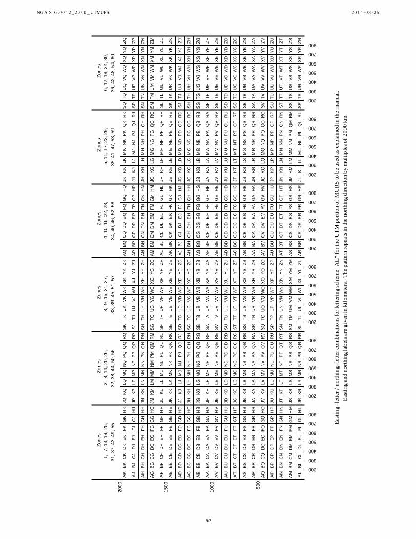
AL

AM

AN

AP

AQ

AR

AS

AT

AU

AV

AA

AB

AC

AD

AE

AF

AG

AH

AJ

AK

BL

BM

BN

BP

BQ

BR

BS

BT

BU

BV

BA

BB

BC

BD

BE

BF

BG

BH

BJ

BK

CL

CM

CN

CP

CQ

CR

CS

CT

CU

CV

CA

CB

CC

CD

CE

CF

CG

CH

CJ

CK

DL

DM

DN

DP

DQ

DR

DS

DT

DU

DV

DA

DB

DC

DD

DE

DF

DG

DH

DJ

DK

EL

EM

EN

EP

EQ

ER

ES

ET

EU

EV

EA

EB

EC

ED

EE

EF

EG

EH

EJ

EK

FL

FM

FN

FP

FQ

FR

FS

FT

FU

FV

FA

FB

FC

FD

FE

FF

FG

FH

FJ

FK

GL

GM

GN

GP

GQ

GR

GS

GT

GU

GV

GA

GB

GC

GD

GE

GF

GG

GH

GJ

GK

HL

HM

HN

HP

HQ

HR

HS

HT

HU

HV

HA

HB

HC

HD

HE

HF

HG

HH

HJ

HK

JR

JS

JT

JU

JV

JA

JB

JC

JD

JE

JF

JG

JH

JJ

JK

JL

JM

JN

JP

JQ

KR

KS

KT

KU

KV

KA

KB

KC

KD

KE

KF

KG

KH

KJ

KK

KL

KM

KN

KP

KQ

LR

LS

LT

LU

LV

LA

LB

LC

LD

LE

LF

LG

LH

LJ

LK

LL

LM

LN

LP

LQ

MR

MS

MT

MU

MV

MA

MB

MC

MD

ME

MF

MG

MH

MJ

MK

ML

MM

MN

MP

MQ

NR

NS

NT

NU

NV

NA

NB

NC

ND

NE

NF

NG

NH

NJ

NK

NL

NM

NN

NP

NQ

PR

PS

PT

PU

PV

PA

PB

PC

PD

PE

PF

PG

PH

PJ

PK

PL

PM

PN

PP

PQ

QR

QS

QT

QU

QV

QA

QB

QC

QD

QE

QF

QG

QH

QJ

QK

QL

QM

QN

QP

QQ

RR

RS

RT

RU

RV

RA

RB

RC

RD

RE

RF

RG

RH

RJ

RK

RL

RM

RN

RP

RQ

SL

SM

SN

SP

SQ

SR

SS

ST

SU

SV

SA

SB

SC

SD

SE

SF

SG

SH

SJ

SK

TL

TM

TN

TP

TQ

TR

TS

TT

TU

TV

TA

TB

TC

TD

TE

TF

TG

TH

TJ

TK

UL

UM

UN

UP

UQ

UR

US

UT

UU

UV

UA

UB

UC

UD

UE

UF

UG

UH

UJ

UK

VL

VM

VN

VP

VQ

VR

VS

VT

VU

VV

VA

VB

VC

VD

VE

VF

VG

VH

VJ

VK

WL

WM

WN

WP

WQ

WR

WS

WT

WU

WV

WA

WB

WC

WD

WE

WF

WG

WH

WJ

WK

XL

XM

XN

XP

XQ

XR

XS

XT

XU

XV

XA

XB

XC

XD

XE

XF

XG

XH

XJ

XK

YL

YM

YN

YP

YQ

YR

YS

YT

YU

YV

YA

YB

YC

YD

YE

YF

YG

YH

YJ

YK

ZL

ZM

ZN

ZP

ZQ

ZR

ZS

ZT

ZU

ZV

ZA

ZB

ZC

ZD

ZE

ZF

ZG

ZH

ZJ

ZK

AR

AS

AT

AU

AV

AA

AB

AC

AD

AE

AF

AG

AH

AJ

AK

AL

AM

AN

AP

AQ

BR

BS

BT

BU

BV

BA

BB

BC

BD

BE

BF

BG

BH

BJ

BK

BL

BM

BN

BP

BQ

CR

CS

CT

CU

CV

CA

CB

CC

CD

CE

CF

CG

CH

CJ

CK

CL

CM

CN

CP

CQ

DR

DS

DT

DU

DV

DA

DB

DC

DD

DE

DF

DG

DH

DJ

DK

DL

DM

DN

DP

DQ

ER

ES

ET

EU

EV

EA

EB

EC

ED

EE

EF

EG

EH

EJ

EK

EL

EM

EN

EP

EQ

FR

FS

FT

FU

FV

FA

FB

FC

FD

FE

FF

FG

FH

FJ

FK

FL

FM

FN

FP

FQ

GR

GS

GT

GU

GV

GA

GB

GC

GD

GE

GF

GG

GH

GJ

GK

GL

GM

GN

GP

GQ

HR

HS

HT

HU

HV

HA

HB

HC

HD

HE

HF

HG

HH

HJ

HK

HL

HM

HN

HP

HQ

JL

JM

JN

JP

JQ

JR

JS

JT

JU

JV

JA

JB

JC

JD

JE

JF

JG

JH

JJ

JK

KL

KM

KN

KP

KQ

KR

KS

KT

KU

KV

KA

KB

KC

KD

KE

KF

KG

KH

KJ

KK

LL

LM

LN

LP

LQ

LR

LS

LT

LU

LV

LA

LB

LC

LD

LE

LF

LG

LH

LJ

LK

ML

MM

MN

MP

MQ

MR

MS

MT

MU

MV

MA

MB

MC

MD

ME

MF

MG

MH

MJ

MK

NL

NM

NN

NP

NQ

NR

NS

NT

NU

NV

NA

NB

NC

ND

NE

NF

NG

NH

NJ

NK

PL

PM

PN

PP

PQ

PR

PS

PT

PU

PV

PA

PB

PC

PD

PE

PF

PG

PH

PJ

PK

QL

QM

QN

QP

QQ

QR

QS

QT

QU

QV

QA

QB

QC

QD

QE

QF

QG

QH

QJ

QK

RL

RM

RN

RP

RQ

RR

RS

RT

RU

RV

RA

RB

RC

RD

RE

RF

RG

RH

RJ

RK

SR

SS

ST

SU

SV

SA

SB

SC

SD

SE

SF

SG

SH

SJ

SK

SL

SM

SN

SP

SQ

TR

TS

TT

TU

TV

TA

TB

TC

TD

TE

TF

TG

TH

TJ

TK

TL

TM

TN

TP

TQ

UR

US

UT

UU

UV

UA

UB

UC

UD

UE

UF

UG

UH

UJ

UK

UL

UM

UN

UP

UQ

VR

VS

VT

VU

VV

VA

VB

VC

VD

VE

VF

VG

VH

VJ

VK

VL

VM

VN

VP

VQ

WR

WS

WT

WU

WV

WA

WB

WC

WD

WE

WF

WG

WH

WJ

WK

WL

WM

WN

WP

WQ

XR

XS

XT

XU

XV

XA

XB

XC

XD

XE

XF

XG

XH

XJ

XK

XL

XM

XN

XP

XQ

YR

YS

YT

YU

YV

YA

YB

YC

YD

YE

YF

YG

YH

YJ

YK

YL

YM

YN

YP

YQ

ZR

ZS

ZT

ZU

ZV

ZA

ZB

ZC

ZD

ZE

ZF

ZG

ZH

ZJ

ZK

ZL

ZM

ZN

ZP

ZQ

200

300

400

500

600

700

800

200

300

400

500

600

700

800

200

300

400

500

600

700

800

200

300

400

500

600

700

800

200

300

400

500

600

700

800

200

300

400

500

600

700

800

50

0

10

00

15

00

20

00

Zo

ne

s

1,

7,

13,

19,

25,

31,

37,

43,

49,

55

Zo

ne

s

2,

8,

14,

20,

26,

32,

38,

44,

50,

56

Zo

ne

s

3,

9,

15,

21,

27,

33,

39,

45,

51,

57

Zo

ne

s

4,

10,

16,

22,

28,

34,

40,

46,

52,

58

Zo

ne

s

5,

11,

17,

23,

29,

35,

41,

47,

53,

59

Zo

ne

s

6,

12,

18,

24,

30,

36,

42,

48,

54,

60

Easti

ng

-le

ttern

ort

hin

g-

lett

er

co

mb

inati

on

sfo

rle

tteri

ng

sch

em

e"A

L"

for

the

UT

Mp

ort

ion

of

MG

RS

tob

eu

sed

as

ex

pla

ined

inth

em

an

ual.

Easti

ng

an

dn

ort

hin

gla

bels

are

giv

en

ink

ilo

mete

rs.

Th

ep

att

ern

rep

eats

inth

en

ort

hin

gd

irecti

on

by

mu

ltip

les

of

20

00

km

.

NGA.SIG.0012_2.0.0_UTMUPS 2014-03-25

50

12. Topics in MGRS

The agenda of this document is the programming logic needed by the software developer. For MGRS, this is covered

in Section 11 — in one sense, covered completely. But it is prudent to take notice of some related issues, and this is

done here.

� 12.1 Formal definition of MGRS

Section 11 adopts a formal point of view, i.e. MGRS is merely a respelling of UTM or UPS coordinates truncated to

the desired precision. If the administrative rules (Subsections 7.4 or 10.4) were in effect when the UTM or UPS

coordinates were produced, they remain in effect when these coordinates are converted to MGRS. If the UTM or UPS

coordinates were produced outside the administrative rules, they can yet be converted to MGRS provided they satisfy

the inequalities for x and y given for the relevant lettering scheme, i.e. the inequalities in Subsections 11.2, 11.3

(implied), 11.10 and 11.11.

If the UTM or UPS coordinates x, y are both multiples of the desired MGRS precision, 105- n (see Subsection 11.6),

then the double conversion UTM ® MGRS ® UTM yields the original coordinates x, y exactly. With no change in

the desired precision, the double conversion MGRS ® UTM ® MGRS yields the original MGRS string. Likewise for

UPS in place of UTM. All this is true when keeping to the principles of Section 11.


The intended usage of MGRS is meant to comply with the administrative rules of Subsections 7.4 and 10.4.

At some level of the software hierarchy, the MGRS conversion routines should be written in accordance with Section

11. This will allow the crossing of an administrative-rule boundary when necessary or when convenient and allowed.

At a higher level, the administrative rules may be enforced in software. The goal is to keep UTM/UPS synchronized

with MGRS. In any situation, the administrative rules should be applied to both or neither; they should not be applied

to only one.

� 12.3 Rounding v. truncating

The intended usage of UTM and UPS coordinates for the calculating or recording of positions complies with the usual

rounding rules of science and engineering. When a precise coordinate, e.g. x = 512 378 m, is to be converted to a less

precise coordinate, e.g. x = 512 380 m or x = 512 400 m, the operation is rounding, not dropping of digits (truncating).

For UTM (and UPS) conversions to MGRS, the operation is truncating, not rounding (see Section 11). Continuing the

above example, x = 512 378 m becomes x = 512 370 m (easting digits 1237) or x = 512 300 m (easting digits 123).

For the reverse conversion, i.e. MGRS to UTM or MGRS to UPS, if the requirement is for the best UTM or UPS

position rather than for a defined area’s bottom-left corner (discussed next), one-half the precision should be added to

the result of the Section 11 conversion. For example, if the given easting digits are 1237, the meaning of those digits

is a 10 meter interval from (say) x = 512 370 m to x = 512 380 m and the appropriate value of x would be x = 512 375

m.

� 12.4 Point v. area

MGRS is also an area identification scheme. If there are n easting digits (with the same number of northing digits),

the MGRS string defines a square in the UTM or UPS plane whose side is 105- n meters and whose bottom left corner

is the UTM or UPS equivalent of the MGRS string (using Section 11 for the conversion). For non-polar areas, the

bottom left corner is the southwest corner.

The administrative rules are amended to allow some MGRS strings as area identifiers that would not be allowed as

point identifiers. Point vice area is an important distinction. Here is an example: The administrative limits for UTM

zone (-53) are 132 deg £ Λ < 138 deg. Point 53ELR2520014100 lies east of 132°E and is compliant. It belongs to

area 53ELR2514, whose southwest corner is point 53ELR2514 or point 53ELR2500014000 (to use a consistent

precision for points, in this example). Almost all of area 53ELR2514 lies east of 132°E. But the corner point 53EL-

R2500014000 lies west of 132°E and is therefore non-compliant. (See the figure in this subsection). Zone (-53)

should not be used for this point. Its administratively correct specification is point 52EFA7482914007 in the next

zone westward, i.e. zone (-52). But no good will come of this conversion. String 52EFA7482914007 has the wrong

precision to identify the desired area (1000-meter square) and truncating it to 52EFA7414 (the desired precision)

defines a different area. (This is an example of a general principle: it is impossible to simultaneously specify an area

of the earth by UTM zone (-52) grid-lines and by UTM zone (-53) grid-lines, even if the administrative rules are

completely abandoned). Therefore the administrative rules are amended to say that although “53ELR2514” is not

allowed as the specification of a point, area 53ELR2514 shall mean the portion of this 1000-meter square east of

132°E.

NGA.SIG.0012_2.0.0_UTMUPS 2014-03-25

51

The administrative rules are amended to allow some MGRS strings as area identifiers that would not be allowed as

point identifiers. Point vice area is an important distinction. Here is an example: The administrative limits for UTM

zone (-53) are 132 deg £ Λ < 138 deg. Point 53ELR2520014100 lies east of 132°E and is compliant. It belongs to

area 53ELR2514, whose southwest corner is point 53ELR2514 or point 53ELR2500014000 (to use a consistent

precision for points, in this example). Almost all of area 53ELR2514 lies east of 132°E. But the corner point 53EL-

R2500014000 lies west of 132°E and is therefore non-compliant. (See the figure in this subsection). Zone (-53)

should not be used for this point. Its administratively correct specification is point 52EFA7482914007 in the next

zone westward, i.e. zone (-52). But no good will come of this conversion. String 52EFA7482914007 has the wrong

precision to identify the desired area (1000-meter square) and truncating it to 52EFA7414 (the desired precision)

defines a different area. (This is an example of a general principle: it is impossible to simultaneously specify an area

of the earth by UTM zone (-52) grid-lines and by UTM zone (-53) grid-lines, even if the administrative rules are

completely abandoned). Therefore the administrative rules are amended to say that although “53ELR2514” is not

allowed as the specification of a point, area 53ELR2514 shall mean the portion of this 1000-meter square east of

132°E.

25000

25200

25400

25600

25800

26000

14000

14200

14400

14600

14800

15000

1000-meter square 53ELR2514 (gray) with intersection by meridian 132E (red)

� 12.5 Latitude band letter — efficiency — northern hemisphere

Because various characteristics of MGRS are unhelpful to analytical work (see Subsection 11.8), this document

suggests (but does not mandate) the following division of labor between MGRS and UTM/UPS when both are under

consideration. UTM/UPS should be be used for calculations, analytical work, and storage & retrieval of geographic

information; MGRS should be limited to notations on maps and charts, displays on end-user devices and person-to-

person or person-to-machine communication. Therefore, there would not seem to be a great need for efficiency in the

conversion algorithms between UTM/UPS and MGRS, as large data sets that would consume computer resources

should already be stored in UTM or UPS coordinates.

The above notwithstanding, there could be occasions where these conversion algorithms need to be efficient. The

UPS-to-MGRS algorithm and its inverse present no issues. The UTM-to-MGRS algorithm and it inverse, however,

could be improved for efficiency. The issue is the latitude band letter.

For the UTM-to-MGRS conversion, rather than always execute the UTM-to-Lon./Lat. algorithm to obtain the latitude

and thus the latitude band letter, the software should invoke the following table for the northern hemisphere. For each

parallel circle, the table provides two staircase-like functions that envelope the parallel — one on its north side; the

other on its south side. This allows a table look-up to complete the latitude band letter determination for the vast

majority of cases. All x and y values in the table are kilometers on the UTM plane. For the MGRS-to-UTM conver-

sion, this table obviates the need for an execution of the UTM-to-Lon./Lat. algorithm. (See the examples in Subsec-

tion 12.7). The table is valid for any reference ellipsoid listed in Section 4.

NGA.SIG.0012_2.0.0_UTMUPS 2014-03-25

52

y-value for y-value for y-value for y-value for

Lat. 500 x 600 600 x 700 700 x 800 800 x 900

(deg) ( km ) ( km ) ( km ) ( km )

Latitude band X

72 7992 7999 8011 8029

-------------------------------------------------------------

72 7988 7990 7997 8009

Latitude band W

64 7099 7104 7112 7123

-------------------------------------------------------------

64 7096 7097 7102 7110

Latitude band V

56 6208 6211 6217 6225

-------------------------------------------------------------

56 6205 6206 6210 6215

Latitude band U

48 5318 5320 5325 5331

-------------------------------------------------------------

48 5315 5316 5319 5323

Latitude band T

40 4429 4431 4434 4439

-------------------------------------------------------------

40 4427 4427 4429 4433

Latitude band S

32 3541 3543 3545 3549

-------------------------------------------------------------

32 3540 3540 3542 3544

Latitude band R

24 2655 2656 2658 2660

-------------------------------------------------------------

24 2653 2654 2655 2657

Latitude band Q

16 1770 1770 1771 1773

-------------------------------------------------------------

16 1768 1768 1769 1770

Latitude band P

8 885 885 886 887

-------------------------------------------------------------

8 884 884 884 885

Latitude band N

0 0 0 0 0

-------------------------------------------------------------

(A subroutine to convert Lon./Lat. to MGRS by combining the guidance in several sections of this document will not

need efficiency improvements like the above. The latitude is a given input item; the latitude band letter is easily

determined by Subsection 11.7).

� 12.6 Latitude band letter — efficiency — symmetry of tables

On the other side of the line x = 500 000, symmetry is applied as if the headings of the tables in Subsections 12.5 and

12.8 were:


Lat. 400 x 500 300 x 400 200 x 300 100 x 200

(deg) ( km ) ( km ) ( km ) ( km )

� 12.7 Latitude band letter — efficiency — examples

To convert x, y = 705 000, 1 765 123, use the column 700 km £ x < 800 km and find that y = 1 765 123 is safely in

band P because it is south of y = 1769 km and north of y = 886 km.

To convert x, y = 705 000, 1 769 123, which is the point displaced 4000 meters more in northing, the UTM-to-

Lon./Lat. algorithm will have to be executed because y = 1 769 123 lies between y = 1769 km and y = 1771 km.

Let 31SFR1500042887 be given as an MGRS string for an ellipsoid that uses lettering scheme “AA”. This example

finds the corresponding UTM coordinates. The UTM zone is Z = +31. The easting letter is “F” which by the tables

of Subsection 11.2 represents 6, i.e. 6 ´ 105 = 600 000 meters. Add the easting digits to get x = 615 000. The northing

letter is “R”, which by the same tables of Subsection 11.2 represents 15, i.e. 15 ´ 105meters, which is understood to

stand for 1 500 000 + 2 000 000 k meters for k = 0, 1, 2, 3, or 4 (to be determined). Add the northing digits to get

y = 1 542 887 + 2 000 000 k. In other words, the candidates for y are 1 542 887, 3 542 887, 5 542 887, 7 542 887 and

9 542 887, which ambiguity is to be resolved by the latitude band letter “S”. Consulting the table in Subsection 12.5

under column 600 km £ x < 700 km, we see that y = 3 542 887 lies inside the expanded limits of band S, i.e.

y = 3540 km to y = 4431 km. Therefore, y = 3 542 887.

NGA.SIG.0012_2.0.0_UTMUPS 2014-03-25

53

To convert x, y = 705 000, 1 765 123, use the column 700 km £ x < 800 km and find that y = 1 765 123 is safely in

band P because it is south of y = 1769 km and north of y = 886 km.

To convert x, y = 705 000, 1 769 123, which is the point displaced 4000 meters more in northing, the UTM-to-

Lon./Lat. algorithm will have to be executed because y = 1 769 123 lies between y = 1769 km and y = 1771 km.

Let 31SFR1500042887 be given as an MGRS string for an ellipsoid that uses lettering scheme “AA”. This example

finds the corresponding UTM coordinates. The UTM zone is Z = +31. The easting letter is “F” which by the tables

of Subsection 11.2 represents 6, i.e. 6 ´ 105 = 600 000 meters. Add the easting digits to get x = 615 000. The northing

letter is “R”, which by the same tables of Subsection 11.2 represents 15, i.e. 15 ´ 105meters, which is understood to

stand for 1 500 000 + 2 000 000 k meters for k = 0, 1, 2, 3, or 4 (to be determined). Add the northing digits to get

y = 1 542 887 + 2 000 000 k. In other words, the candidates for y are 1 542 887, 3 542 887, 5 542 887, 7 542 887 and

9 542 887, which ambiguity is to be resolved by the latitude band letter “S”. Consulting the table in Subsection 12.5

under column 600 km £ x < 700 km, we see that y = 3 542 887 lies inside the expanded limits of band S, i.e.

y = 3540 km to y = 4431 km. Therefore, y = 3 542 887.

� 12.8 Latitude band letter — efficiency — southern hemisphere

The table for the southern hemisphere follows. It is valid for any reference ellipsoid listed in Section 4.


Lat. 500 x 600 600 x 700 700 x 800 800 x 900

(deg) ( km ) ( km ) ( km ) ( km )

0 10000 10000 10000 10000

Latitude band M

-8 9116 9116 9116 9115

-------------------------------------------------------------

-8 9115 9115 9114 9113

Latitude band L

-16 8232 8232 8231 8230

-------------------------------------------------------------

-16 8230 8230 8229 8227

Latitude band K

-24 7347 7346 7345 7343

-------------------------------------------------------------

-24 7345 7344 7342 7340

Latitude band J

-32 6460 6460 6458 6456

-------------------------------------------------------------

-32 6459 6457 6455 6451

Latitude band H

-40 5573 5573 5571 5567

-------------------------------------------------------------

-40 5571 5569 5566 5561

Latitude band G

-48 4685 4684 4681 4677

-------------------------------------------------------------

-48 4682 4680 4675 4669

Latitude band F

-56 3795 3794 3790 3785

-------------------------------------------------------------

-56 3792 3789 3783 3775

Latitude band E

-64 2904 2903 2898 2890

-------------------------------------------------------------

-64 2901 2896 2888 2877

Latitude band D

-72 2012 2010 2003 1991

-------------------------------------------------------------

-72 2008 2001 1989 1971

Latitude band C

-------------------------------------------------------------

� 12.9 Latitude band letter — leniency

Many software programs allow some leniency in the latitude band letter during the MGRS-to-UTM conversion

process. The example of Subsection 11.8 is a case in point. In that example, the string 13VFC4967108679 is invalid

by the rules of Section 11, and would have to be rejected and not converted. (An error message would be helpful).

Opposed to this, both 13UFC4967108679 (valid) and 13VFC4967108679 (invalid) convert to Z = +13,

x, y = 649 671, 6 208 679 by the application of the latitude-band-letter efficiency table of Subsection 12.5 (and see

Sub-subsection 12.7.3). So, it would seem that the error in the Latitude band letter is recoverable in this case and

maybe shouldn’t be called an error. Again, this leniency is outside the definition of MGRS in Section 11.

NGA.SIG.0012_2.0.0_UTMUPS 2014-03-25

54

Many software programs allow some leniency in the latitude band letter during the MGRS-to-UTM conversion

process. The example of Subsection 11.8 is a case in point. In that example, the string 13VFC4967108679 is invalid

by the rules of Section 11, and would have to be rejected and not converted. (An error message would be helpful).

Opposed to this, both 13UFC4967108679 (valid) and 13VFC4967108679 (invalid) convert to Z = +13,

x, y = 649 671, 6 208 679 by the application of the latitude-band-letter efficiency table of Subsection 12.5 (and see

Sub-subsection 12.7.3). So, it would seem that the error in the Latitude band letter is recoverable in this case and

maybe shouldn’t be called an error. Again, this leniency is outside the definition of MGRS in Section 11.

Of the choice to be lenient or not, many system developers adopt the more generous view and apply it to cases more

aggressively in the wrong latitude band than the above example. If this practice is to be allowed, this document

should offer some guidance. The purpose of the latitude band letter — the only purpose with respect to the algorithms

at issue — is to resolve the 2 000 000 k meters ambiguity in the northing where k is one of the integers 0, 1, 2, 3, or 4.

The design of a leniency rule has to include the requirement that a candidate MGRS string that is off by one latitude

band letter but otherwise valid converts to the intended UTM coordinates.

� 12.10 Latitude band letter — leniency rule

For the UTM to MGRS conversion, there is no leniency — the latitude band letter is to be computed correctly by the

foregoing principles. For the MGRS to UTM conversion, the following leniency rule is to be applied to decipher a

candidate MGRS string: Give each “latitude band” (hereafter, bloated latitude band) a much larger area. Refer to the

tables in Subsections 12.5 and 12.8. For each latitude band other than C and X, start with the pair of staircase func-

tions immediately above and below it. Modify these to create new limits for the band. Modify the y-values to move

the northern limit of each band another 400 000 meters further north and to move the southern limit 400 000 meters

further south. For latitude bands C and X, expand 200 000 meters in the direction toward the Equator. Then if none

of the 5 choices for value of y (see above, where k equals 0,1,2,3 or 4) falls into the bloated latitude band correspond-

ing to the given letter, the candidate MGRS string is invalid and cannot be converted.

The above leniency rule is quite lax, while yet retaining the ability to resolve the 2 000 000 k meters ambiguity in the

northings. For quality assurance of imported geographic data, analysts may devise and perform more stringent tests to

filter-out candidate MGRS data for further review before acceptance.

� 12.11 MGRS–UTM hybrid

Nothing in this document prohibits DoD components and their contractors from employing a mixture of UTM and

MGRS information for displays on end-user equipment or for margin notes on printed maps, etc. Prominent in this

category is the following MGRS–UTM hybrid:

(i) UTM zone number in absolute value

(ii) MGRS latitude band letter

(iii) UTM x-coordinate (Easting) to precision 1 meter

(iv) UTM y-coordinate (Northing) to precision 1 meter

As an example, here is a point specified three ways:

UTM (stored internally): Zone 31, x 345009, y 6700123

MGRS: 31VCH4500900123

MGRS–UTM hybrid: 31V, 345009mE, 6700123mN

Details of the format and wording of margin notes and device displays are outside the scope of this document. See

[11] for guidance and these remarks: From the information-content point-of-view, the MGRS latitude band letter

belongs to MGRS, not UTM. For greater readability the above example appends “mE” for meters east and “mN” for

meters north, as shown. Also for readability, UTM may show “31 north” in place of “+31”, but the capital letters “N”

and “S” may not be used as abbreviations for north and south.

Here is another example. It is 10, 000, 000 meters less in northing, and on the other side of the Equator:



MGRS: 31JCH4500900123

MGRS–UTM hybrid: 31J, 345009mE, 6700123mN

The suffix “mN” for “meters North” is to be used for points on both sides of the Equator.

NGA.SIG.0012_2.0.0_UTMUPS 2014-03-25

55

13. MGRS Quick-Start

The guidance given to this point has assumed that the routines for processing MGRS are part of a larger package of

map projection and coordinate conversion software to include UTM and UPS and, more generally, transverse Merca-

tor and polar stereographic routines. When these are available, the additional code to implement MGRS is merely a

few table look-ups (see Sections 11 and 12; note some exceptions), and MGRS is efficiently linked to UTM and UPS.

Modern positioning (e.g. GPS technology) is in pursuit of centimeter accuracy. This manual’s conversions between

Lon./Lat. and UTM support such a goal but MGRS does not. Consequently and for other reasons, the development of

transverse Mercator and UTM in this document is more extensive than needed for MGRS. UTM is recommended for

serious analytical work with grid coordinates but some software developers might need only MGRS. For them, this

section provides some short-cuts. Some short cuts are for the reader; some are for the machine.

This section provides guidance for converting directly between longitude/latitude and MGRS. Only the UTM portion

of MGRS is considered. Only the WGS 84 ellipsoid is considered. The administrative rules apply. The chosen

precision for MGRS will be 1 meter. For aspects of MGRS outside this agenda, see the full treatment in Sections 11

and 12 and the earlier sections to which they refer. Sections 1, 2, and 3 are prerequisite.

� 13.1 Given Lon./Lat. compute MGRS

The procedure to compute MGRS from longitude and latitude is given as a series of steps to be followed in the order

given.

13.1.1) Let LonD and LatD be the given longitude and latitude in decimal degrees of the point to be converted.

Points north of the Equator have positive latitudes; points south have negative. Points east of the nominal Greenwich

meridian have positive longitudes; points west have negative.

If LatD 80 or LatD 84, the point cannot be converted to the UTM portion of MGRS and an error message

should be issued.

13.1.2) The set of allowed central meridians in degrees is the list 177 to 177 by increment of 6. Find the

member of this list closest to LonD and call it CMdeg. The UTM absolute zone number is calculated

absZ CMdeg 183 6.

13.1.3) If LatD 56 and 0 LonD 42, an adjustment to CMdeg from Step 13.1.2 might be required. (See

Subsection 7.5).

13.1.4) Divide LatD by 8 and discard the remainder, i.e. compute FloorLatD 8. Enter the following table

with the result to find the latitude band letter.

-10 -9 -8 -7 -6 -5 -4 -3 -2 -1 0 1 2 3 4 5 6 7 8 9 10

C D E F G H J K L M N P Q R S T U V W X X

13.1.5) Convert the angles in Steps 13.1.1 and 13.1.2 to radians. In other words, compute Lon LonD Pi 180and Lat LatD Pi 180 and CM CMdeg Pi 180.

13.1.6) Next is needed the conformal latitude Χ or, rather, its cosine and sine. See Subsection 2.8 and use the formu-

las there. The value to use for e, the eccentricity is e = f 2 - f where f = 1 298.257223563.

13.1.7) Perform the computations of Eq. (3.8) to obtain the quantities u and v using Lon CM for the value of

in those equations.

13.1.8) Compute cos2 v, cos4 v, sin2 v, sin4 v, directly or with help from Eq. (3.10)

13.1.9) Compute cosh2 u, cosh4 u, sinh2 u, sinh4 u, directly or with help from Eq. (3.12)

NGA.SIG.0012_2.0.0_UTMUPS 2014-03-25

56

13.1.9) Compute cosh2 u, cosh4 u, sinh2 u, sinh4 u, directly or with help from Eq. (3.12)

13.1.10) Perform the computations of Eq. (3.7) in the following abbreviated way. (This is possible because the

computational accuracy required in this situation is merely one meter.)

x = R4 u + a2 sinh2 u cos2 v + a4 sinh4 u cos4 v y = R4 v + a2 cosh2 u sin2 v + a4 cosh4 u sin4 v

13.1.11) Compute the UTM easting and northing as follows, where yeq is 0 if Lat 0 and is 10 000 000 otherwise:

xutm = 0.9996 x + 500 000 truncated to 1 meter

yutm = 0.9996 y + yeq truncated to 1 meter

13.1.12) Apply lettering scheme “AA” (see Subsection 11.2) to the numbers xutm, yutm found in Step 13.1.11 with

Z there equal to absZ here.

13.1.13) The MGRS string consists of the absolute zone number absZ from Step 13.1.2, followed by the latitude

band letter from Step 13.1.4, followed by the easting-letter obtained in Step 13.1.12, followed by the northing letter

obtained also in Step 13.1.12, followed the 5 least significant digits of xutm obtained in Step 13.1.11, followed finally

by the 5 least significant digits of yutm obtained also in Step 13.1.11.

� 13.2 Given MGRS, compute Lon./Lat.

The procedure to compute the longitude and latitude from MGRS is given as a series of steps to be followed in the

order given.

13.2.1) Check that the given MGRS string consists of 1 or 2 digits (the UTM absolute zone number absZ) followed

by a letter in the range C-X (the latitude band letter) followed by another letter (easting-letter) followed by another

letter (northing-letter) followed by 5 digits (easting-digits xdigits) followed finally by 5 more digits (northing-digits

ydigits). None of the letters may be “I” or “O”. Other checks will arise in what follows.

13.2.2) The central meridian in degrees is computed CMdeg 183 6 absZ. Its radian equivalent is

CM CMdeg Pi 180.

13.2.3) Apply lettering scheme “AA” (see Subsection 11.2) in reverse to the easting-letter and northing-letter from

Step 13.2.1 to obtain their numerical equivalents xletter and yletter. Successful table look-ups should yield answers in

the ranges 1 £ xletter £ 8 and 0 £ yletter £ 19. Take Z there to be equal to absZ here.

13.2.4) Combine the above pieces of information according to the following equations to obtain the UTM easting xutm

and the UTM northing yutm.

xutm = 100 000 xletter + xdigits

yprelim = 100 000 yletter + ydigits

yutm = 2 000 000 yband + yprelim

where yband is one of the numbers 0,1,2,3 or 4 to be determined. (The five candidates for yband yield five candidates

for yutm.)

13.2.5) Determine yband by one of these two methods. (i) Enter the latitude band efficiency tables of Subsections 12.5

and 12.8 with xutm and the latitude band letter and the 5 candidate values of yutm to see which one fits. Or, (ii) consult

the following table (from Subsection 11.13) to obtain the one or two possible values of yband , compute yutm for each

value and apply the remaining steps of this subsection to each yutm candidate to see which latitude (final answer) fits

the given latitude band.


1 1 1 2 2 3 3 4 4 4 0 0 0 1 1 2 2 3 3 3

0 0 1 2 3 1 2 3 4 4

NGA.SIG.0012_2.0.0_UTMUPS 2014-03-25

57


1 1 1 2 2 3 3 4 4 4 0 0 0 1 1 2 2 3 3 3

0 0 1 2 3 1 2 3 4 4

13.2.6) Compute the transverse Mercator coordinates x and y as follows, where yeq is 10 000 000 if the latitude band

letter is among C-M and is 0 if it is among N-X:

x = xutm - 500 000 0.9996y = yutm - yeq 0.9996

13.2.7) Apply the formulas and logic of Subsection 3.5 to the values for x, y from Step 13.2.6. The formulas for u

and v may be shortened as follows:

u =x

R4

+ b2 sinh2 x

R4

cos2 y

R4

+ b4 sinh4 x

R4

cos4 y

R4

v =y

R4

+ b2 cosh2 x

R4

sin2 y

R4

+ b4 cosh4 x

R4

sin4 y

R4

NGA.SIG.0012_2.0.0_UTMUPS 2014-03-25

58

14. United States National Grid

This section explains the United States National Grid (USNG). It is included in this document because it is almost the

same as MGRS.

� 14.1 Definition of USNG

Like MGRS, the United States National Grid (USNG) [5] is built on UTM coordinates (eastings and northings), a

lettering scheme for multiples of 100 000 meters, and latitude bands. It adopted almost all of the rules of the UTM

portion of MGRS given in Section 11. The sole exception concerns the choice between lettering schemes “AA” and

“AL” in a particular circumstance. The following table tells which scheme is used for which ellipsoid/datum:

Ellipsoid MGRS USNG

GRS 80 ellipsoid (used by the NAD 83 datum) AA AA

Clark 1866 ellipsoid (used by the NAD 27 datum) AL AA

For NAD 83, the MGRS and USNG systems are the same. For NAD 27, they are not.

� 14.2 USNG example

It is a goal of the U.S. federal government to convert all the land maps of the U.S. from NAD 27 to NAD 83. When

that happens, USNG will be identical to MGRS in usage because NAD 27 will be obsolete. In the meantime, a point

in Nevada at 117°W, 39°N (NAD 27) has these competing representations, differing at the northing letter. Note “P” v.

“D”.

MGRS: 11SNP0000016568 (NAD 27)

USNG: 11SND0000016568 (NAD 27)

^

NGA.SIG.0012_2.0.0_UTMUPS 2014-03-25

59

This page is intentionally blank,

NGA.SIG.0012_2.0.0_UTMUPS 2014-03-25

60

15. Diagrams for UTM, UPS and MGRS

The following pages are some plots that illustrate principles in this document. The depictions are informative for this

purpose only. For guidance on the portrayal of grids and graticules on DoD standard products, see [11].

Figure Description

Figure 1 Overview of UTM plane

(a) eastings and northings if zone Z > 0

(b) eastings and northings if zone Z < 0

(c) relation to parallels

(d) MGRS representable portion

(e) MGRS latitude bands

(f) meridians at ±3°

Figure 2 UTM plane — north zones — 8400 kmN to 9800 kmN







Figure 9 UTM plane — south zones — 8600 kmN to 10000 kmN







Figure 16 UPS plane — north zone — x < 2000 kmE, y > 2000 kmN

Figure 17 UPS plane — north zone — x > 2000 kmE, y > 2000 kmN

Figure 18 UPS plane — north zone — x < 2000 kmE, y < 2000 kmN

Figure 19 UPS plane — north zone — x > 2000 kmE, y < 2000 kmN

Figure 20 UPS plane — south zone — x < 2000 kmE, y > 2000 kmN

Figure 21 UPS plane — south zone — x > 2000 kmE, y > 2000 kmN

Figure 22 UPS plane — south zone — x < 2000 kmE, y < 2000 kmN

Figure 23 UPS plane — south zone — x > 2000 kmE, y < 2000 kmN

NGA.SIG.0012_2.0.0_UTMUPS 2014-03-25

61

0 50

0

10

00

-10000

-8000

-6000

-4000

-2000

0

2000

4000

6000

8000

10000

a

0 50

0

10

00

0

2000

4000

6000

8000

10000

12000

14000

16000

18000

20000

b

0 50

0

10

00

0

2000

4000

6000

8000

0 or

10000

2000

4000

6000

8000

10000

c

80°S

72°S

64°S

56°S

48°S

40°S

32°S

24°S

16°S

8°S

0°N

8°N

16°N

24°N

32°N

40°N

48°N

56°N

64°N

72°N

80°N

Figure 1. UTM plane for generic zone Z. All eastings and northings are in kilometers. (a) Northings if Z 0.

(b) Northings if Z 0. (c) Northings in common practice with parallels every 8° and the north and south poles.

NGA.SIG.0012_2.0.0_UTMUPS 2014-03-25

62

0 50

0

10

00

0

2000

4000

6000

8000

0 or

10000

2000

4000

6000

8000

10000

d

0 50

0

10

00

0

2000

4000

6000

8000

0 or

10000

2000

4000

6000

8000

10000

C

D

E

F

G

H

J

K

L

M

N

P

Q

R

S

T

U

V

W

X

72°S

64°S

56°S

48°S

40°S

32°S

24°S

16°S

8°S

0°N

8°N

16°N

24°N

32°N

40°N

48°N

56°N

64°N

72°N

e

0 50

0

10

00

0

2000

4000

6000

8000

0 or

10000

2000

4000

6000

8000

10000

f

Figure 1 (continued). (d) Portion of the UTM plane representable in MGRS, (e) MGRS latitude bands with their bounding parallels,

(f) Meridians at ±3° of the central meridian and parallels at 80°S and 84°N, which are basic to the administrative rules for UTM and MGRS.

NGA.SIG.0012_2.0.0_UTMUPS 2014-03-25

63

10

0

30

0

50

0

70

0

90

0

8400

8600

8800

9000

9200

9400

9600

9800

76°N

78°N

80°N

82°N

84°N

86°N 88°N

30°E30°W

45°E45°W

60°E60°W

15°E15°W 0° 3°3° 6°6° 9°9° 12°12°

Fig. 2. UTM plane for arbitrary zone Z 0 showing grid-lines, meridians, and parallels. All eastings and

northings are in kilometers. Longitudes are relative to the unspecified central meridian. The region repre-

sentable in MGRS is shaded.

NGA.SIG.0012_2.0.0_UTMUPS 2014-03-25

64

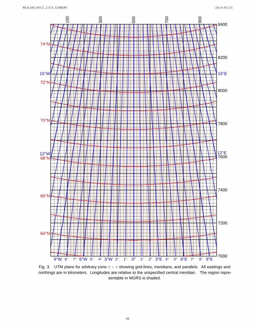
10

0

30

0

50

0

70

0

90

0

7000

7200

7400

7600

7800

8000

8200

8400

64°N

66°N

68°N

70°N

72°N

74°N

12°E12°W

15°E15°W

3°E3°W 6°E6°W 9°E9°W 0° 1°1° 2°2° 4°4° 5°5° 7°7° 8°8°




NGA.SIG.0012_2.0.0_UTMUPS 2014-03-25

65

10

0

30

0

50

0

70

0

90

0

5600

5800

6000

6200

6400

6600

6800

7000

52°N

54°N

56°N

58°N

60°N

62°N

9°E9°W

3°E3°W 6°E6°W 0° 1°1° 2°2° 4°4° 5°5° 7°7°




NGA.SIG.0012_2.0.0_UTMUPS 2014-03-25

66

10

0

30

0

50

0

70

0

90

0

4200

4400

4600

4800

5000

5200

5400

5600

38°N

40°N

42°N

44°N

46°N

48°N

50°N

6°E6°W

3°E3°W 0° 1°1° 2°2° 4°4° 5°5°




NGA.SIG.0012_2.0.0_UTMUPS 2014-03-25

67

10

0

30

0

50

0

70

0

90

0

2800

3000

3200

3400

3600

3800

4000

4200

26°N

28°N

30°N

32°N

34°N

36°N

3°E3°W 0° 1°1° 2°2° 4°4°




NGA.SIG.0012_2.0.0_UTMUPS 2014-03-25

68

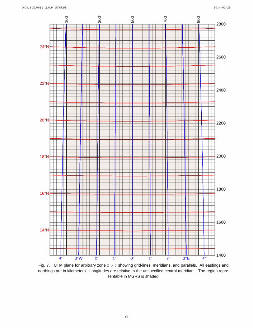
10

0

30

0

50

0

70

0

90

0

1400

1600

1800

2000

2200

2400

2600

2800

14°N

16°N

18°N

20°N

22°N

24°N

3°E3°W 0° 1°1° 2°2° 4°4°




NGA.SIG.0012_2.0.0_UTMUPS 2014-03-25

69

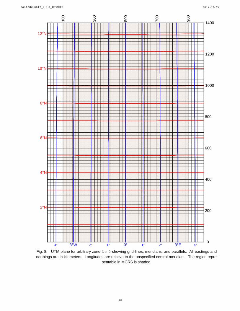
10

0

30

0

50

0

70

0

90

0

0

200

400

600

800

1000

1200

1400

2°N

4°N

6°N

8°N

10°N

12°N

3°E3°W 0° 1°1° 2°2° 4°4°




NGA.SIG.0012_2.0.0_UTMUPS 2014-03-25

70

10

0

30

0

50

0

70

0

90

0

8600

8800

9000

9200

9400

9600

9800

10 000

12°S

10°S

8°S

6°S

4°S

2°S

3°E3°W

3°E3°W

0°

1°1° 2°2° 4°4°




NGA.SIG.0012_2.0.0_UTMUPS 2014-03-25

71

10

0

30

0

50

0

70

0

90

0

7200

7400

7600

7800

8000

8200

8400

8600

24°S

22°S

20°S

18°S

16°S

14°S

3°E3°W

3°E3°W

0°

1°1° 2°2° 4°4°




NGA.SIG.0012_2.0.0_UTMUPS 2014-03-25

72

10

0

30

0

50

0

70

0

90

0

5800

6000

6200

6400

6600

6800

7000

7200

36°S

34°S

32°S

30°S

28°S

26°S

3°E3°W

3°E3°W

0°

1°1° 2°2° 4°4°




NGA.SIG.0012_2.0.0_UTMUPS 2014-03-25

73

10

0

30

0

50

0

70

0

90

0

4400

4600

4800

5000

5200

5400

5600

5800

50°S

48°S

46°S

44°S

42°S

40°S

38°S

6°E6°W

6°E6°W 3°E3°W

3°E3°W

0°

1°1° 2°2° 4°4° 5°5°




NGA.SIG.0012_2.0.0_UTMUPS 2014-03-25

74

10

0

30

0

50

0

70

0

90

0

3000

3200

3400

3600

3800

4000

4200

4400

62°S

60°S

58°S

56°S

54°S

52°S

9°E9°W

9°E9°W 3°E3°W 6°E6°W

6°E6°W

0°

1°1° 2°2° 4°4° 5°5° 7°7°




NGA.SIG.0012_2.0.0_UTMUPS 2014-03-25

75

10

0

30

0

50

0

70

0

90

0

1600

1800

2000

2200

2400

2600

2800

3000

74°S

72°S

70°S

68°S

66°S

64°S

12°E12°W

12°E12°W

15°E15°W

15°E15°W 3°E3°W

3°E3°W

6°E6°W

6°E6°W

9°E9°W

9°E9°W

0°

1°1° 2°2° 5°5° 7°7°




NGA.SIG.0012_2.0.0_UTMUPS 2014-03-25

76

10

0

30

0

50

0

70

0

90

0

200

400

600

800

1000

1200

1400

1600

84°S

82°S

80°S

78°S

76°S

88°S86°S

30°E30°W

45°E45°W

60°E60°W

15°E15°W 3°3° 6°6° 9°9° 12°12°




NGA.SIG.0012_2.0.0_UTMUPS 2014-03-25

77

80

0

10

00

12

00

14

00

16

00

18

00

20

00

2000

2200

2400

2600

2800

3000

3200

90°W

105°W

120°W

135°W

150°W

165°W

18

0°W

88°N86°N84°N82°N80°N

78°N

76°N

YRH

YRJ

YRK

YRL

YRM

YRN

YRP

YSH

YSJ

YSK

YSL

YSM

YSN

YSP

YTH

YTJ

YTK

YTL

YTM

YTN

YTP

YUH

YUJ

YUK

YUL

YUM

YUN

YUP

YXH

YXJ

YXK

YXL

YXM

YXN

YXP

YYH

YYJ

YYK

YYL

YYM

YYN

YYP

YZH

YZJ

YZK

YZL

YZM

YZN

YZP

Fig. 16. UPS plane for Z 1 (north zone) showing grid-lines, meridians, parallels and MGRS lettering.

All eastings and northings are in kilometers.

NGA.SIG.0012_2.0.0_UTMUPS 2014-03-25

78

20

00

22

00

24

00

26

00

28

00

30

00

32

00

2000

2200

2400

2600

2800

3000

3200

90°E

105°E

120°E

135°E

150°E

165°E

18

0°E

88°N 86°N 84°N 82°N 80°N

78°N

76°N

ZAH

ZAJ

ZAK

ZAL

ZAM

ZAN

ZAP

ZBH

ZBJ

ZBK

ZBL

ZBM

ZBN

ZBP

ZCH

ZCJ

ZCK

ZCL

ZCM

ZCN

ZCP

ZFH

ZFJ

ZFK

ZFL

ZFM

ZFN

ZFP

ZGH

ZGJ

ZGK

ZGL

ZGM

ZGN

ZGP

ZHH

ZHJ

ZHK

ZHL

ZHM

ZHN

ZHP

ZJH

ZJJ

ZJK

ZJL

ZJM

ZJN

ZJP



NGA.SIG.0012_2.0.0_UTMUPS 2014-03-25

79

80

0

10

00

12

00

14

00

16

00

18

00

20

00

800

1000

1200

1400

1600

1800

2000

60°W

75°W

90°W

0°W

15°W

30°W

45°W

88°N86°N84°N82°N80°N

78°N

76°N

YRA

YRB

YRC

YRD

YRE

YRF

YRG

YSA

YSB

YSC

YSD

YSE

YSF

YSG

YTA

YTB

YTC

YTD

YTE

YTF

YTG

YUA

YUB

YUC

YUD

YUE

YUF

YUG

YXA

YXB

YXC

YXD

YXE

YXF

YXG

YYA

YYB

YYC

YYD

YYE

YYF

YYG

YZA

YZB

YZC

YZD

YZE

YZF

YZG



NGA.SIG.0012_2.0.0_UTMUPS 2014-03-25

80

20

00

22

00

24

00

26

00

28

00

30

00

32

00

800

1000

1200

1400

1600

1800

2000

60°E

75°E

90°E

0°E

15°E

30°E

45°E

88°N 86°N 84°N 82°N 80°N

78°N

76°N

ZAA

ZAB

ZAC

ZAD

ZAE

ZAF

ZAG

ZBA

ZBB

ZBC

ZBD

ZBE

ZBF

ZBG

ZCA

ZCB

ZCC

ZCD

ZCE

ZCF

ZCG

ZFA

ZFB

ZFC

ZFD

ZFE

ZFF

ZFG

ZGA

ZGB

ZGC

ZGD

ZGE

ZGF

ZGG

ZHA

ZHB

ZHC

ZHD

ZHE

ZHF

ZHG

ZJA

ZJB

ZJC

ZJD

ZJE

ZJF

ZJG



NGA.SIG.0012_2.0.0_UTMUPS 2014-03-25

81

80

0

10

00

12

00

14

00

16

00

18

00

20

00

2000

2200

2400

2600

2800

3000

3200

90°W

75°W

60°W

45°W

30°W

15°W

0°W

88°S86°S84°S82°S80°S

78°S

76°S

AJN

AJP

AJQ

AJR

AJS

AJT

AJU

AJV

AJW

AJX

AJY

AJZ

AKN

AKP

AKQ

AKR

AKS

AKT

AKU

AKV

AKW

AKX

AKY

AKZ

ALN

ALP

ALQ

ALR

ALS

ALT

ALU

ALV

ALW

ALX

ALY

ALZ

APN

APP

APQ

APR

APS

APT

APU

APV

APW

APX

APY

APZ

AQN

AQP

AQQ

AQR

AQS

AQT

AQU

AQV

AQW

AQX

AQY

AQZ

ARN

ARP

ARQ

ARR

ARS

ART

ARU

ARV

ARW

ARX

ARY

ARZ

ASN

ASP

ASQ

ASR

ASS

AST

ASU

ASV

ASW

ASX

ASY

ASZ

ATN

ATP

ATQ

ATR

ATS

ATT

ATU

ATV

ATW

ATX

ATY

ATZ

AUN

AUP

AUQ

AUR

AUS

AUT

AUU

AUV

AUW

AUX

AUY

AUZ

AXN

AXP

AXQ

AXR

AXS

AXT

AXU

AXV

AXW

AXX

AXY

AXZ

AYN

AYP

AYQ

AYR

AYS

AYT

AYU

AYV

AYW

AYX

AYY

AYZ

AZN

AZP

AZQ

AZR

AZS

AZT

AZU

AZV

AZW

AZX

AZY

AZZ

Fig. 20. UPS plane for Z 1 (south zone) showing grid-lines, meridians, parallels and MGRS lettering.


NGA.SIG.0012_2.0.0_UTMUPS 2014-03-25

82

20

00

22

00

24

00

26

00

28

00

30

00

32

00

2000

2200

2400

2600

2800

3000

3200

90°E

75°E

60°E

45°E

30°E

15°E

0°E

88°S 86°S 84°S 82°S 80°S

78°S

76°S

BAN

BAP

BAQ

BAR

BAS

BAT

BAU

BAV

BAW

BAX

BAY

BAZ

BBN

BBP

BBQ

BBR

BBS

BBT

BBU

BBV

BBW

BBX

BBY

BBZ

BCN

BCP

BCQ

BCR

BCS

BCT

BCU

BCV

BCW

BCX

BCY

BCZ

BFN

BFP

BFQ

BFR

BFS

BFT

BFU

BFV

BFW

BFX

BFY

BFZ

BGN

BGP

BGQ

BGR

BGS

BGT

BGU

BGV

BGW

BGX

BGY

BGZ

BHN

BHP

BHQ

BHR

BHS

BHT

BHU

BHV

BHW

BHX

BHY

BHZ

BJN

BJP

BJQ

BJR

BJS

BJT

BJU

BJV

BJW

BJX

BJY

BJZ

BKN

BKP

BKQ

BKR

BKS

BKT

BKU

BKV

BKW

BKX

BKY

BKZ

BLN

BLP

BLQ

BLR

BLS

BLT

BLU

BLV

BLW

BLX

BLY

BLZ

BPN

BPP

BPQ

BPR

BPS

BPT

BPU

BPV

BPW

BPX

BPY

BPZ

BQN

BQP

BQQ

BQR

BQS

BQT

BQU

BQV

BQW

BQX

BQY

BQZ

BRN

BRP

BRQ

BRR

BRS

BRT

BRU

BRV

BRW

BRX

BRY

BRZ



NGA.SIG.0012_2.0.0_UTMUPS 2014-03-25

83

80

0

10

00

12

00

14

00

16

00

18

00

20

00

800

1000

1200

1400

1600

1800

2000

120°W

105°W

90°W

18

0°W

165°W

150°W

135°W

88°S86°S84°S82°S80°S

78°S

76°S

AJA

AJB

AJC

AJD

AJE

AJF

AJG

AJH

AJJ

AJK

AJL

AJM

AKA

AKB

AKC

AKD

AKE

AKF

AKG

AKH

AKJ

AKK

AKL

AKM

ALA

ALB

ALC

ALD

ALE

ALF

ALG

ALH

ALJ

ALK

ALL

ALM

APA

APB

APC

APD

APE

APF

APG

APH

APJ

APK

APL

APM

AQA

AQB

AQC

AQD

AQE

AQF

AQG

AQH

AQJ

AQK

AQL

AQM

ARA

ARB

ARC

ARD

ARE

ARF

ARG

ARH

ARJ

ARK

ARL

ARM

ASA

ASB

ASC

ASD

ASE

ASF

ASG

ASH

ASJ

ASK

ASL

ASM

ATA

ATB

ATC

ATD

ATE

ATF

ATG

ATH

ATJ

ATK

ATL

ATM

AUA

AUB

AUC

AUD

AUE

AUF

AUG

AUH

AUJ

AUK

AUL

AUM

AXA

AXB

AXC

AXD

AXE

AXF

AXG

AXH

AXJ

AXK

AXL

AXM

AYA

AYB

AYC

AYD

AYE

AYF

AYG

AYH

AYJ

AYK

AYL

AYM

AZA

AZB

AZC

AZD

AZE

AZF

AZG

AZH

AZJ

AZK

AZL

AZM



NGA.SIG.0012_2.0.0_UTMUPS 2014-03-25

84

20

00

22

00

24

00

26

00

28

00

30

00

32

00

800

1000

1200

1400

1600

1800

2000

120°E

105°E

90°E

18

0°E

165°E

150°E

135°E

88°S 86°S 84°S 82°S 80°S

78°S

76°S

BAA

BAB

BAC

BAD

BAE

BAF

BAG

BAH

BAJ

BAK

BAL

BAM

BBA

BBB

BBC

BBD

BBE

BBF

BBG

BBH

BBJ

BBK

BBL

BBM

BCA

BCB

BCC

BCD

BCE

BCF

BCG

BCH

BCJ

BCK

BCL

BCM

BFA

BFB

BFC

BFD

BFE

BFF

BFG

BFH

BFJ

BFK

BFL

BFM

BGA

BGB

BGC

BGD

BGE

BGF

BGG

BGH

BGJ

BGK

BGL

BGM

BHA

BHB

BHC

BHD

BHE

BHF

BHG

BHH

BHJ

BHK

BHL

BHM

BJA

BJB

BJC

BJD

BJE

BJF

BJG

BJH

BJJ

BJK

BJL

BJM

BKA

BKB

BKC

BKD

BKE

BKF

BKG

BKH

BKJ

BKK

BKL

BKM

BLA

BLB

BLC

BLD

BLE

BLF

BLG

BLH

BLJ

BLK

BLL

BLM

BPA

BPB

BPC

BPD

BPE

BPF

BPG

BPH

BPJ

BPK

BPL

BPM

BQA

BQB

BQC

BQD

BQE

BQF

BQG

BQH

BQJ

BQK

BQL

BQM

BRA

BRB

BRC

BRD

BRE

BRF

BRG

BRH

BRJ

BRK

BRL

BRM



NGA.SIG.0012_2.0.0_UTMUPS 2014-03-25

85

16. References

1. Bugayevskiy, Lev and Snyder, John (1995), Map Projections —A Reference Manual, Taylor and Francis, London.

2. Defense Mapping Agency (1990, limited reprint 1996), Datums, Ellipsoids, Grids, and Grid Reference Systems,

DMA Technical Manual 8358.1, Washington D.C.

3. Defense Mapping Agency (1989), The Universal Grids: Universal Transverse Mercator (UTM) and Universal Polar

Stereographic (UPS), DMA Technical Manual 8358.2, Washington, D.C.

4. Engsager, K., and Poder K. (2007, August). “A highly accurate world wide algorithm for the transverse Mercator

mapping (almost)”, in Proceedings of XXIII International Cartographic Conference (ICC2007) (pp. 4-10).

5. Federal Geographic Data Committee (2001), United States National Grid, FGDC-STD-011-2001, Reston, VA.

6. International Association of Oil and Gas Producers (2012), Coordinate Conversions and Transformations including

Formulas, OGP Publication 373-7-2 — Geomatics Guidance Note number 7 part 2 — revised July 2012.

7. International Standards Organization (2006), ISO 19111:2006(E), Geographic information — Spatial referencing

by coordinates.

8. International Standards Organization (2009), ISO/IEC 18026:2009(E), Ed. 2, Spatial Reference Model,

http://standards.iso.org/ittf/PubliclyAvailableStandards.

9. Karney, Charles (2011), Transverse Mercator with an accuracy of a few nanometers, Journal of Geodesy, Vol. 85,

No.8, Pp 475-485.

10. Moritz, H. (2000), Geodetic Reference System 1980, Journal of Geodesy, 74 (1) 128-162.

11. National Geospatial-Intelligence Agency, (2013, draft), Universal grids and grid reference systems, NGA

Standardization Document NGA.STND.0037_2.0_GRIDS, Washington, D.C.

12. National Imagery and Mapping Agency (1997), Department of Defense World Geodetic System 1984 — Its

Definition and Relationships with Local Geodetic Systems, NIMA Technical Report 8350.2 Third Edition, National

Imagery and Mapping Agency, Washington, D.C.

13. Petit, Gérard and Luzum, Brian. (eds.), IERS Conventions (2010), IERS Technical Note No. 36, International Earth

Rotation and Reference Systems Service (IERS), Verlag des Bundesamts für Kartographie und Geodäsie, Frankfurt

am Main, 2010.

14. Poder, Knud and Engsager, Karsten (1998), Some conformal mappings and transformations for geodesy and

topographic cartography. (Vol. 6). Kort & Matrikelstyrelsen.

15. Rollins, Craig (2006), Auxiliary latitude formulas: finding the coefficients numerically and symbolically, Wolfram

Library Archive, http://library.wolfram.com/infocenter/Conference/6431.

16. Snyder, John P. (1987), Map Projections — A Working Manual, U.S. Geological Survey Professional Paper 1395,

U.S. Government Printing Office, Washington D.C.

17. Thomas, Paul D. (1952), Conformal Projections in Geodesy and Cartography, Special Publication No. 251, U.S.

Department of Commerce, Washington D.C.

18. Wolfram, Stephen (2003), The Mathematica Book, 5th Ed., Wolfram Media, Champaign, Illinois.

NGA.SIG.0012_2.0.0_UTMUPS 2014-03-25

86

Documents

The Universal Grids and the Transverse Mercator …earth-info.nga.mil/GandG/update/coordsys/resources/NGA...The Universal Grids and the Transverse Mercator and Polar Stereographic