Embed Size (px)
Citation preview
THE UNIVERSITY OF HULL
Ensemble-characterisation of Satellite Rainfall Uncertainty and its Impacts
on the Hydrological Modelling of a Sparsely Gauged Basin in Western
Africa
being a Thesis submitted for the Degree of Doctor of Philosophy
in the University of Hull
by
Christopher James Skinner MPhys Geog
March 2013

Declaration
I confirm that this is my own work and the use of all material from other
sources has been properly and fully acknowledged.
Christopher James Skinner

Acknowledgements
My first thank you, of course, goes to my supervisor, Tim Bellerby; I can only
aspire to your intelligence and I am grateful for the many patient hours of
support, guidance and assistance, without which I would have been lost. Thank
you also to David Grimes, whose inspiration and many years of work provided
the foundations on which this research is built on – David’s feedback on this
thesis was sorely missed. Thank you to those who have also offered guidance
throughout this thesis – Graham, Dave and Tom.
A thank you to the TAMSAT team at the University of Reading, whose work
informed this thesis. A special thank you to Helen Greatrex for her support and
assistance – thank you for answering all my emails!
A thank you to Alison Hook for finding the advert for the studentship, and
making me promise to mention you in the acknowledgements when I wrote
them. Thank you to Thorwald Stein for guidance with the application, and the
sofa to sleep on when I was visiting Reading.
It has been a privilege to be a part of the Department of Geography,
Environment and Earth Sciences, University of Hull. Thank you to all of those
who have made my time thoroughly enjoyable – Karen, Tim, Carl, Baoli,
Michelle, Steve, Joe, Chris, Leiping, Jordan, Sarah, Lucy, Sally, plus the many
other participants of ‘Pub Wednesday’ over the years.

Thank you to my church family at Hull Vineyard, especially Jeremy and Elaine,
and the members of my small group, whose love, prayers and encouragement
have been invaluable. Thank you to my family for their love and support, and for
given me plenty of excuses to meet you at Krispie Kreme. Finally, a huge thank
you and much love to my amazing wife, Amy. Thank you for being you, for
being my rock through my PhD, encouraging me, proof reading and bringing me
crisps and liquorice.

Abstract
Many areas of the planet lack the infrastructure required to make accurate and
timely estimations of rainfall. This problem is especially acute in sub-Saharan
Africa, where a paucity of rain recording radar and sufficiently dense raingauge
networks combine with highly variable rainfall, a reliance on agriculture that is
predominantly rain fed and systems that are prone to flooding and drought.
Satellite Rainfall Estimates (SRFE) are useful as they can provide additional
spatial and temporal information to drive various downstream environmental
models and early warning systems (EWS). However, when operating at higher
spatial and temporal resolutions SRFE contain large uncertainties which
propagate through the downstream models.
This thesis uses the TAMSAT1 SRFE algorithm developed by Teo (2006) to
estimate the rainfall over a large, data sparse and heterogenous catchment in
the Senegal Basin. The uncertainty within the TAMSAT1 SRFE is represented
using a set of ensemble estimates, each unique but equiprobable based on the
full conditional distribution of the recorded rainfall, produced using the TAMSIM
algorithm, also developed by Teo (2006). The ensemble rainfall estimates were
then used in turn to drive a Pitman Rainfall-Runoff model of the catchment
hydrology.
The use of ensemble rainfall estimates was shown to be incompatible with the
pre-calibrated parameter values for the hydrological model. A novel approach,
the EnsAll method, was developed to calibrate the hydrological model which
incorporated each individual ensemble member. The EnsAll calibrated model

showed the greatest skill when driven by the ensemble rainfall estimates and
little bias. A comparison of the hydrographs produced from TAMSIM ensemble
rainfall estimates and that from an ensemble of perturbed TAMSAT1 estimates
showed that the full spatio-temporally distributed method used by TAMSIM is
superior to a simpler perturbation method for characterizing SRFE uncertainty.
Overall, the SRFE used were shown to outperform the rainfall estimates
produced from the sparse raingauge network as a hydrological model driver.
However, they did demonstrate a lack of ability to represent the large
interseasonal variations in rainfall resulting in large systematic biases. These
biases were observed propagating directly to the modelled hydrological ouput.

Contents
Chapter 1 - Introduction 1
1.1 Satellite Rainfall Estimation and Hydrological Modelling 1
1.2 Using Satellites to Estimate Rainfall in Africa 9
1.3 Thesis Aims 11
1.4 Experimental Process and Thesis Plan 12
Chapter 2 - Satellite Rainfall Applications in Hydrological Modelling 18
2.1 Introduction 18
2.2 Dealing with Input Uncertainty in Hydrological Models 18
2.3 Satellite Rainfall Estimation 24
2.4 Satellite Rainfall Uncertainty Characterisation 31
2.5 Hydrological Modelling and Calibration 37
2.6 Summary 49
Chapter 3 - Study Area and Context 51
3.1 Introduction 51
3.2 The Problem in Context 52
3.3 Description of the Study Area 67
3.4 Previous Studies Relating to the Bakoye Catchment 82
3.5 Available Data 86
3.6 Summary 103
Chapter 4 - Methodology - Spatial Interpolation 105
4.1 Introduction 105
4.2 Spatial Interpolation and the Double Kriging (DK) Method 105
4.3 Implementation of the DK Method 111
4.3.1 Introduction 111
4.3.2 Calibration 112
4.3.3 Validation 119
4.4 Summary 129
Chapter 5 - Methodology - Ensemble Representation of Satellite Rainfall Uncertainty
131
5.1 Introduction 131
5.2 TAMSAT1 131
5.3 TAMSIM 136
5.4 Implementation 141
5.4.1 Introduction 141
5.4.2 Calibration 142

5.4.3 Validation of the TAMSAT1 SRFE 148
5.4.4 Implementation of TAMSIM 152
5.5 Summary 155
Chapter 6 - Methodology - Hydrological Modelling 156
6.1 Introduction 156
6.2 The Pitman Model 156
6.3 The Shuffled Complex Evolution method implemented at the University of Arizona (SCE-UA)
160
6.4 Calibration of the Pitman Model using SCE-UA 166
6.5 Summary 170
Chapter 7 - Validation of the Ensemble Representation of the Daily Senegal Basin Rain Field
171
7.1 Introduction 171
7.2 Daily Senegal Basin Rain Field 172
7.3 Influence of Uncertainty on the Estimates 187
7.4 Conclusions 198
Chapter 8 - The Influence of SRFE Uncertainty on Hydrological Model Output
202
8.1 Introduction 202
8.2 Ensemble Parameterisation of the Pitman Model 204
8.3 The Propagation of Input Uncertainty through the Pitman Model
208
8.4 Comparison with a Perturbation Method 227
8.5 Conclusions 239
Chapter 9 - The Influence of Ensemble Rainfall Input on the Calibration of the Pitman Model
243
9.1 Introduction 243
9.2 Pitman Model Behaviours 244
9.3 Variability of Parameter Values for an Ensemble Driven Pitman Model
250
9.4 Conclusions 278
Chapter 10 - Discussions 281
10.1 Key Results 281
10.2 Issues and Recommendations 286
Chapter 11 - Conclusions 300
Bibliography 304


Chapter 1 - Introduction
1
1 Introduction
1.1 - Satellite Rainfall Estimation and Hydrological Modelling
Rainfall estimation is most accurately and timely performed using ground
instrumentation - such as raingauges or radar – however, in many areas of the
planet – such as sub-Saharan Africa – large regions are covered only by sparse
raingauge networks and often with no rain recording radar. Satellite Rainfall
Estimates (SRFE) offer a substitute for the ground instrumentation, able to
estimate rainfall at a high spatial and temporal resolution at real-time or near
real-time, but these estimates contain high uncertainties that need to be
measured and characterised. The use of ensemble estimates of rainfall
provides a useful method of representing the uncertainty in the SRFE which can
then be used as a direct input for downstream applications, such as crop yield
or hydrological models. When using a deterministic hydrological model, driven
by an ensemble input, an appropriate calibration of the parameters needs to be
established.
Gebremichael and Hossain (2010) described how the terms “satellite rainfall”
and “surface hydrology” have been well established over decades of research,
yet the combination of the two, which was termed “satellite rainfall applications

Chapter 1 - Introduction
2
for surface hydrology”, was a relatively new topic. Although Gebremichael and
Hossain (2010) acknowledged that SRFE have been used to drive models
representing surface hydrology processes, the two fields have only marginally
intersected during their development.
The connection of the two fields and the development of the new topic led
Gebremichael and Hossain (2010) to propose a series of questions pertinent to
this new discipline:
1. Which SRFE is best for a specific application?
2. What is the optimum SRFE resolution for a specific application?
3. How much uncertainty is there within the SRFE and how does this
propagate to the surface hydrology application?
4. Where can data be acquired for research and operational applications?
5. How are SRFE developed and how do they vary from one another?
While each of the five questions posed are important to this field, the focus of
this thesis is an attempt to address the third question: the issue of quantifying
SRFE uncertainty and the impact it has on modelling the hydrology of a river
basin.
SRFE contain significant uncertainties, principally because they rely upon an
indirect relationship between rainfall and the data recorded by the satellite, most
often thermal infrared imagery of cloud top temperature, or microwave back
scatter. This leads to three main uncertainties in any SRFE:

Chapter 1 - Introduction
3
1. When it is raining
2. Where it is raining
3. How much it is raining – i.e., the rain rate
The full extent and implications of SRFE uncertainty are discussed in Chapters
2 and 3, but the Tropical Applications of Meteorology using SATellites
(TAMSAT) method provides an example of how the three types of uncertainty
emerge within a SRFE. Dugdale et al. (1991) described how TAMSAT
estimates rainfall using a calibrated relationship between the temperatures of
cloud tops – as recorded by Meteosat thermal infrared (TIR) sensors – and
rainfall – as recorded by ground raingauges. In order to do so it has to makes
two assumptions:
1. All clouds are convective
2. All convective clouds are raining
These assumptions come from the area-time integral (ATI) method that informs
the TAMSAT rainfall estimation, which relies on a statistical relationship
between cold cloud duration, coverage and areal rainfall (Kebe et al. 2004).
The use of ensemble estimates provides an effective way of characterising and
representing the uncertainty in rain fields. A notable experiment in this area is
the Hydrological Ensemble Prediction Experiment (HEPEX), led by the National
Oceanic and Atmospheric Administration (NOAA) (Schaake et al., 2007). The

Chapter 1 - Introduction
4
goal of HEPEX is to produce an end-to-end system that accounts for all the
uncertainties inherent within streamflow forecasting. A conceptual diagram of
one possible system is shown in Figure 1.1.
Figure 1.1 – A conceptual diagram of a possible end-to-end meteorological-hydrological
ensemble streamflow system. The system allows for all sources of uncertainty to be
accounted for (from Schaake et al., 2007).

Chapter 1 - Introduction
5
Although HEPEX is not explicitly aimed at the use of SRFE - the weather-
climate ensembles shown in Figure 1.1 are derived from forecasts using
satellite and radar data, amongst other sets of data which include SRFE
(Schaake et al., 2007) – the principles and the processes shown in Figure 1.1
are useful for informing research into the use of SRFE in hydrological modelling
and accounting for uncertainties.
The production of an ensemble estimate requires the use of a stochastic
element, where for a rainfall estimate the uncertainty is measured and a random
element is used to produce a multitude of estimates from within these bounds of
uncertainty. A major advantage of the ensemble approach is that it produces
estimates of rainfall that resemble a deterministic estimate allowing for an
almost direct application to a downstream model, often designed to operate
using a single, deterministic input. Ensemble inputs provide an easy and useful
method of demonstrating the propagation of input uncertainty in a hydrological
model, as each can be applied as a separate input and an ensemble of model
outputs can be extracted (Bellerby and Sun, 2005, Germann et al., 2007).
The simplest method of producing an ensemble estimate of rainfall is to perturb
the estimation at each timestep by an amount drawn from a distribution
reflecting the uncertainty. This can be achieved by using either an additive
method, and/or a multiplicative method, where the deterministic estimate is
altered by randomly applying the perturbing factor. For the purpose of this
thesis, all such methods are referred to as perturbation methods.

Chapter 1 - Introduction
6
The major issue with perturbation methods is that they are only capable of
representing the third facet of the main sources of uncertainty previously
detailed for SRFE – the rain rate – and a perturbation method is unable to
account for intermittencies in the rainfall field. In addition, an ensemble estimate
produced using a perturbation estimate is dependent on a deterministic
estimate. An alternative approach for producing ensemble SRFE is the use of a
fully spatio-temporally distributed stochastic approach, such as Bellerby and
Sun (2005), Teo (2006) and Teo and Grimes (2007), which allow for a full
representation of the spatial and temporal intermittencies in the rainfall field as
well as uncertainty about the rainfall rate. These methods are based on the full
conditional distribution of the rainfall in respect to the input data, and therefore
are independent on the deterministic SRFE.
Although there have been previous studies into the impacts of input uncertainty
on hydrological models, many have been limited to stochastic perturbations, of
a given magnitude, of the input, without attempting to fully characterise the error
(McMillan et al., 2011). Given the complex, non-linear, nature of rainfall and
hydrological models, such an approach is not sufficiently detailed, and a critical
research priority must be for a full analysis of rainfall input uncertainty (McMillan
et al., 2011).
Vrugt et al. (2008) provide a good example of how past attempts to bridge the
gaps between SRFE and hydrological modelling have fallen short, despite best
intentions. The Differential Evolution Adaptive Metropolis (DREAM) method was
used to determine Bayesian statistics about the model parameters when being

Chapter 1 - Introduction
7
driven by rainfall inputs that characterised the input error. The input error was
characterised using multipliers on individual storm events.
Hong et al. (2006) used the Precipitation Estimation from Remote Sensed
Information using Artificial Neural Network – Cloud Classification System
(PERSIANN-CSS) algorithm to drive the HyMod hydrological model. The input
uncertainty was characterised by calculating error bounds at 10 rainfall intensity
bands, and producing ensemble members from within these bounds. Although
the rain intensity-dependent error approach employed is an improvement on a
simpler multiplier method, such as Vrugt et al. (2008), it still does not
adequately reflect the uncertainty within SRFE as it only addresses rainfall rate
uncertainty.
The approach of using perturbation methods to try and characterise input
uncertainty, as used by Vrugt et al. (2008) and Hong et al. (2006), is, as
suggested by McMillan et al. (2011), not adequate. Although it simulates
possible uncertainty inherent in estimating rainfall rate, and total input volume, it
cannot simulate the uncertainties inherent in estimating both the timing of
rainfall and its location.
Bellerby and Sun (2005) presented a fully spatio-temporally distributed
stochastic ensemble approach for characterising uncertainty in a multi-platform
SRFE but, although suitable for such a use, the ensemble outputs were never
used to drive a downstream application. Using a similar method, Teo (2006)
and Teo and Grimes (2007) demonstrated that the TAMSIM algorithm could

Chapter 1 - Introduction
8
successfully characterise the full range of uncertainties within a SFRE. The
approach produced ensemble representations of the rainfall field at daily
timesteps which represented uncertainty around the location, timing and rate of
rainfall. The ensemble outputs were used to drive a crop yield model,
demonstrating the influence of the propagation of input uncertainty. This thesis
proposes the use of the TAMSIM algorithm to produce ensemble rainfall input to
drive a hydrological model, and assess how this full characterisation of
uncertainty propagates through the model.
As highlighted by Gebremichael and Hossain (2010) studies have often
focussed on one aspect of the field when looking at satellite rainfall applications
for surface hydrology. For example, Hossain et al. (2004) characterised the
retrieval and sampling errors within passive microwave (PM) derived products,
and applied this to the TOPMODEL hydrological model which was only
calibrated using a basin average of the rainfall recorded by raingauges.
Although this approach demonstrates how SRFE uncertainty can be
characterised and applied to a surface hydrology model, it does not consider
the surface hydrology facet of the field as the study did not attempt to separate
the sensitivity of TOPMODEL to the error, from its sensitivity to its input-
parameter interactions.
The key issue that continues to separate the two fields of satellite rainfall
estimation and hydrology is a matter of assumptions. Vrugt et al. (2008)
suggested that a traditional approach to hydrological model calibration makes
the assumption that both input and output data are free from uncertainty, and

Chapter 1 - Introduction
9
that any errors are due to parameter set selection. Similar assumptions are
made in the approach to hydrometeorology, with the assumption being that all
uncertainty is within the SRFE, and any error in the hydrological model is
negligible.
The use of ensemble inputs for the same temporal period is likely to have an
influence on the calibration of a hydrological model, with input uncertainties
potentially interacting with model structure and parameter uncertainty in
complex and non-Gaussian ways. The traditional approach to calibration of a
hydrological model uses the minimisation of one or more error scores (objective
functions), against a single deterministic input, and for the use with ensemble
inputs there remains an unanswered question of what constitutes an
appropriate calibration. This thesis demonstrates how calibration against
deterministic estimates of rainfall, for the study period, produce
parameterisations of the Pitman model that are not suitable for use with
ensemble inputs, and proposes the EnsAll parameterisation that incorporates
each individual ensemble member – this parameterisation showed superior
performance to the alternative methods and little bias.
1.2 – Using Satellites to Estimate Rainfall in Africa
SRFEs are becoming increasingly important in rainfall monitoring and prediction
in Africa. The African continent poses a particular problem to many fields, in
that many regions face severe insecurity in regards to food provision and water
resources - which are likely to increase with predicted climatic changes

Chapter 1 - Introduction
10
(Commission for Africa, 2010) – and driven by variations in rainfall. Such
extreme events in rainfall can lead to devastating floods and droughts, such as
the ‘Horn of Africa’ drought which struck the eastern Sahel region in 2011
(Hillier and Dempsey, 2012).
Although Early Warning Systems (EWS) are in place to help predict and
manage potential humanitarian disasters resulting from the extreme variations
in rainfall, such as the Famine Early Warning Systems Network (FEWSNET)
(Hillier and Dempsey, 2012), they rely on timely and accurate rainfall estimation.
This second issue, one of data availability, is another significant challenge
facing those working in Africa, with Washington et al. (2006) describing the
provision of ground instrumentation recording rainfall in Africa as historically
poor, with few radar and sparse raingauge networks.
To fill this void many researchers have turned to using SRFE, as these can
provide increased spatial and temporal resolution, and can be provided in near
real-time. Examples of services that provide daily or dekadal (10-day total)
rainfall estimates for the whole of Africa are the Climate Prediction Centre
(CPC) and TAMSAT, both of which are freely accessible on the internet (Teo,
2006).

Chapter 1 - Introduction
11
1.3 – Thesis Aims
The main aims of this thesis can be summarised as:
1. Characterising the SRFE uncertainty over a large, data sparse,
heterogenous area, using a fully spatio-temporally distributed stochastic
ensemble method.
2. Investigating how this uncertainty in the SRFE propagates through as
uncertainty in a hydrological model.
3. Investigating how the use of ensemble rainfall inputs interacts with the
calibration of a hydrological model.
In addressing the three aims above, there exists a number of research
questions that require addressing in order to inform the research. Principal
amongst these are:
a) To what extent do the ensemble SRFE reproduce the characteristics of
the rainfall fields for the study area?
b) How does the uncertainty in the SRFE manifest – error, spatial bias,
temporal bias?
c) How can a hydrological model be best calibrated for use with ensemble
rainfall inputs?

Chapter 1 - Introduction
12
d) With an appropriate calibration, which of the sources of uncertainty are
evident in the hydrological model output when driven by the ensemble
rainfall inputs?
e) How does the use of a fully spatio-temporally distributed method of
uncertainty characterisation compare to a perturbation method for
modelling input uncertainty in a hydrological model?
f) What influence does using ensemble rainfall inputs have on the
hydrological model calibration and behaviour?
1.4 – Experimental Process and Thesis Plan
The choice of study area, data and methods that are used in this thesis position
the experimentation directly in their operational context. The double Kriging,
TAMSAT1 and TAMSIM methods have been tested and validated,
experimentally and for the Gambian catchment, in Teo (2006) and this thesis
does not seek to reproduce this, rather it seeks to use those methods in an area
where they might be used operationally. The study area chosen is large,
heterogeneous and very sparsely covered by ground instrumentation used to
measure rainfall, which will produce an abundance of uncertainties that can be
measured. It should be noted that the data used will not provide the best
representation of the methods employed – this has been the domain of previous
studies – the aim of this thesis is to characterise the uncertainty in a SRFE and
investigate how it propagates through a downstream application, not to show

Chapter 1 - Introduction
13
how well a SRFE performs as a driver for the model, which has been previously
shown (see Chapter 2). The choice of study area and data will deliberately
stretch the methods adopted to the limits of their performance, as they might be
when used operationally in sub-Saharan Africa.
Chapter 3 will detail the sources of raw data and these are summarised below:
Raingauge data from 81 gauges across the Senegal Basin area for the
period covering 1986-1996.
Discharge data from seven discharge stations, providing mixed coverage
for the period 1986-2005.
Cold Cloud Duration (CCD) data covering the study area for the periods
above, extracted from Meteosat thermal infrared (TIR) data, at a daily
timestep with a spatial resolution of 0.05°.
The experimental process of this thesis can be seen summarised in Figure 1.2.
This details the stages from the collection of the raw raingauge data, and its
interpolation into a grid that is compatible with the satellite CCD data collected.
The satellite data is calibrated using the interpolated raingauge data to produce
a TAMSAT1 deterministic estimate of rainfall, and a TAMSIM (using the SIMU
programme) stochastic ensemble estimate of rainfall. The rainfall estimates,
from the raingauge and satellite data, are used as an input for a lumped
hydrological model, both to drive it and to calibrate it.

Chapter 1 - Introduction
14
Figure 1.2 – Flow chart demonstrating the process used in this thesis, the main steps,
and the methods employed. Blue boxes indicate the input data, green boxes the main
steps and methods, whilst the brown box indicates the output.
The remainder of this thesis demonstrates the fulfilment of the process above.
Chapter 2 investigates the literature associated with the emerging field of
satellite rainfall applications for surface hydrology (Gebremichael and Hossain,
2010), focussing particularly on issues regarding the influence and propagation
of input uncertainty on hydrological modelling when using SRFE.
Chapter 3 discusses the issues raised in this thesis in their geographical context
and the Sahel region. The chapter looks broadly at the pressing need for
accurate environmental models in the area, and in turn the requirement for
timely rainfall estimations to drive these models – the role of uncertainty is

Chapter 1 - Introduction
15
explored, highlighting the importance of accurate and proper uncertainty
characterisation, its clear communication and the implications for risk
management. The Senegal Basin study area, and the Bakoye catchment within
it, are explored focussing on the physical attributes and climate of the area, and
discussing previous relevant studies in the region. Finally the raw data available
to the thesis is described, showing how it reflects the physical characteristics
previously detailed.
Chapter 4 focuses on the spatial interpolation of the raingauge data and the
double Kriging (DK) method used to do this, demonstrating how the method is
superior to ordinary Kriging (OK), both in its ability to account for fractional
rainfall fields but also in its ability to better match the initial raingauge data at
individual gauge locations, and also as an average for the Bakoye catchment.
Chapter 5 highlights the SRFE methods used, showing the calibration of the
both the TAMSAT1 and TAMSIM methods and their use in generating daily
rainfall fields for the Senegal Basin, and the Bakoye catchment average rainfall
estimates.
Chapter 6 demonstrates the hydrological modelling methods used for the thesis,
describing the Pitman lumped conceptual rainfall-runoff (CRR) model and the
Shuffled Complex Evolution (SCE-UA) method used to automatically calibrate it.
It is shown how the automatic calibration method significantly increases the
performance of the Pitman model using a rainfall estimate produced from the
raingauge data.

Chapter 1 - Introduction
16
Chapter 7 describes TAMSIM’s ability to reproduce the underlying spatio-
temporal distributions of the rainfall (as described by the DK raingauge fields)
by observing the 200 ensemble members produced. Its performance is
described at both gauge-pixel (pixels that contain at least one raingauge) and
Bakoye catchment scale. The performance of the TAMSIM ensemble SRFE is
compared against the TAMSAT1 deterministic SRFE, finding that not only is it
able to demonstrate the full bounds of uncertainty, but also when taken as a
whole the ensembles perform better at modelling the underlying rainfall field.
The main sources of uncertainty within the SRFE are explored, showing that the
estimates display significant spatial and temporal biases.
Chapter 8 demonstrates the outcome from the process shown in Figure 1.2,
using the TAMSIM ensemble SRFE to drive an optimised Pitman model of the
Bakoye catchment: the ensemble output discharge data used to produce
hydrographs that show the bounds of the 95% confidence envelope for
discharge which fully reflects the influence of the input uncertainty on the
Pitman model. It is seen that the spatial biases in the TAMSIM ensemble
estimates have been compensated for by the calibration, but significant
temporal biases have been directly propagated into the Pitman model output.
The discharge envelopes are compared to those produced by a simpler
perturbation method on the TAMSAT1 data, highlighting the inadequacy of this
method in fully characterising the propagation of input uncertainty. The chapter
introduces the EnsAll method for calibrating a lumped CRR hydrological model

Chapter 1 - Introduction
17
for use with an ensemble input, demonstrated how the method outperforms all
the alternatives and shows little overall bias.
Chapter 9 focuses specifically on the influence of the input uncertainty on the
calibration of the variable parameters in the Pitman model, and on the resulting
behaviour of the model. The individual calibrations from the TAMSIM ensemble
SRFE are investigated closely, observing the relationships between the spread
of parameter values on model behaviour and performance. It was found that the
uncertainty within the input had little influence on the calibration of the
parameter values, but there was some evidence for equifinality in the model
behaviours.
Chapter 10 discusses the key issues encountered by this thesis, critically
evaluating the analyses undertaken and highlighting the key results and their
implications on the research field. Suggestions are made for appropriate
avenues of future research.
Finally, Chapter 11 concludes the thesis, discussing the major findings.

Chapter 2 – Satellite Rainfall Applications in Hydrological Modelling
18
2 Satellite Rainfall Applications in
Hydrological Modelling
2.1 – Introduction
In Chapter 1, the field of satellite rainfall applications for surface hydrology was
introduced along with a demonstration for the need for a holistic approach to
research into the influence of uncertainty, as highlighted by Gebremichael and
Hossain (2010). This chapter breaks the field down into its component features
and investigates the current state of uncertainty research in each facet.
2.2 – Dealing with Input Uncertainty in Hydrological Models
The issue of observation uncertainty, in particular input uncertainty, is an often
neglected element of hydrological model uncertainty analysis (Vrugt et al.,
2008, Baldasarre and Montanari, 2009). Vrugt et al. (2008) described this issue
within the field of hydrology where the common approach to modelling assumes
that the primary source of uncertainty is associated with parameter values, and
the model calibration, resulting in neglecting the influence of uncertainty within
the rainfall input. Baldasarre and Montanari (2009) agreed with the sentiments

Chapter 2 – Satellite Rainfall Applications in Hydrological Modelling
19
of Vrugt et al. (2008), suggesting that few attempts have been made to assess
the influence of observation uncertainty as it is often regarded as negligible
compared to model structure or parameter uncertainty. Moradkhani et al. (2005)
stated that often the uncertainties associated with inputs, outputs and model
structure are ignored, and assumed to be associated with model parameter
uncertainty.
Michaud and Sorooshian (1994b) suggested that the influence of rainfall error
on hydrological models is undetermined, with some studies showing very little
significance and others showing very marked effects on the modelled output –
although by reducing the raingauge density over a catchment, it was found that
spatial sampling error alone could contribute up to 50% of the difference
between the observed and modelled discharges.
Hughes (1995) suggested the sources of uncertainties in hydrological models
are:
Erroneous data inputs
Poor interpretation of model results
Inadequate or inappropriate modelling of catchment processes
Inadequate modelling of the spatial variability of runoff generation from
rainfall
Inadequate representation of the spatial variability of the rainfall input
Inadequate representation of the temporal variability of the rainfall input
Inadequate representation of the parameter values.

Chapter 2 – Satellite Rainfall Applications in Hydrological Modelling
20
From the list provided by Hughes (1995), three of the potential sources of
uncertainty in hydrological models can be attributed to the rainfall input, and
these can be grouped as input uncertainty, composed of three components:
1. Temporal – differentiating between when it is raining and when it is not
2. Spatial – differentiating between areas where it is raining and where it is
not
3. Rate – the intensity of rainfall where raining
A common approach to representing the input uncertainty in hydrological
models is to use a perturbation method, where the rainfall estimated at each
timestep is perturbed within set bounds, usually a multiplier or an additive
factor. Examples of studies that have employed a perturbation method can be
seen in Butts et al. (2004), Vrugt et al. (2008) and Montanari and Baldasarre
(2013).
The studies listed above vary in nature, for example Butts et al. (2004)
randomly perturbed each estimate by the addition of a value chosen from a
normal distribution with a mean of zero and a standard deviation equal to 50%
of the rainfall estimate for that timestep, producing an ensemble of 200
estimates. Montanari and Baldasarre (2013) perturbed the estimates obtained
by the average of raingauge measurements by adjusting the weighting given to
each gauge in the production of the estimate. The method demonstrated by
Vrugt et al. (2008) was more complex, instead applying multipliers based on the
identification of individual storm events. Both Butts et al. (2004) and Montanari

Chapter 2 – Satellite Rainfall Applications in Hydrological Modelling
21
and Baldasarre (2013) found the representation of input uncertainty showed
little influence on simulated discharges, yet Vrugt et al. (2008) showed their
method acted to remove systematic biases in the rainfall estimates.
Butts et al. (2004) highlighted that there was a requirement for a more complete
representation of the uncertainty within the radar rainfall estimate used, with a
full characterisation of the spatial and temporal uncertainties. This can be said
of each of the methods above, and for all conventional perturbation methods
that can only characterise the rainfall rate aspect of rainfall input uncertainty.
When using areal averages of rainfall it is tempting to do this, as ultimately all
three components of the rainfall uncertainty will be expressed as a rainfall rate
for the timestep over that area, but the methods are limited by their inability to
fully represent the complex nature of rainfall. This was highlighted in McMillan et
al. (2011) who described the requirement for a comprehensive analysis of the
uncertainty due to the complex, non-linear nature of rainfall as a critical
research need. In reference to SRFE, Hossain and Anagnostou (2004)
suggested that simple additive methods of characterising input uncertainty are
insufficient to understand the propagation of the uncertainty through a
hydrological model.
The spatial distribution of rainfall has been shown to be important to
hydrological modelling, with Azimi-Zonooz et al. (1989) arguing that the
accurate determination of storm locations within a watershed is necessary for
hydrological modelling, particularly in the case of localised storm and flood
forecasting. Using a lumped model, Sivaplan et al. (1997) showed that

Chapter 2 – Satellite Rainfall Applications in Hydrological Modelling
22
heterogeneity in rainfall inputs has a significant influence on modelled
discharges. The spatial and temporal variability of rainfall was also highlighted
as an issue needing to be properly addressed by hydrological modellers by
O’Connel and Todini (1996). In a study observing the influence of spatial
resolution and sampling error in the MIKE SHE distributed hydrological model,
Shah et al. (1996) found that the spatial variability of rainfall was particularly
influential on the modelled discharge during dry periods, as soil moisture was
sensitive to the spatial distribution of precipitation.
A study by Xuan et al. (2009) directly applied rainfall forecasts produced by a
numerical weather prediction (NWP) model to a distributed hydrological model.
They used data from a raingauge network to correct storm locations in the
ensembles and found that this improved the modelling of the discharge. Lee et
al. (2012) also observed the importance of spatial distributions of rainfall on
hydrological modelling, by modelling scenarios displaying different temporal and
spatial distributions of the rainfall field and applying them to a distributed
hydrological model.
Tsai et al. (in press 2012) noted that the requirement to account for the spatial
distribution of convective rainfall, which displays a high degree of spatio-
temporal heterogeneity and uncertainty, is particularly acute when it is the key
driver for runoff. They also added that the majority of studies focus on the
impacts of temporal variations to the detriment of the impacts of the spatial
variations of model inputs. Using a reservoir model they demonstrated how the

Chapter 2 – Satellite Rainfall Applications in Hydrological Modelling
23
inclusion of spatial distributions of rainfall improved the performance of a semi-
distributed model, when modelling the impacts of typhoons in Taiwan.
Hong et al. (2006) demonstrated a spatio-temporal method of characterising
rainfall uncertainty within a SRFE. The method worked by binning data from the
PERSIAN-CSS SRFE into spatial aggregation, temporal aggregation and
rainfall rate categories, and providing a reference error value in a contingency
table for each bin – the contingency table was then used to produce ensemble
rainfall estimates. The method was adopted by Moradkhani et al. (2006) to
further investigate the propagation of the input uncertainty on the conceptual
Hydrological MODel (HyMOD), using a sequential data assimilation (SDA)
method to account for all sources of error in hydrological modelling – in
comparison to parameter, the input uncertainty showed a wider range of
uncertainty.
Although the method employed by Hong et al. (2006) and Moradkhani et al.
(2006) does make account of some spatial and temporal details of rainfall
uncertainty and better represents the uncertainty of the input over the fixed
perturbation approach, ultimately it still amounts to applying a multiplier to the
estimates. This method cannot fully represent the uncertainty within the input –
for example, it is unable to predict rainfall where the original SRFE predicts
none and vice versa.
There remains a pressing research requirement for a study into the influence of
the full spectrum of uncertainties within SRFEs on the modelling of hydrological

Chapter 2 – Satellite Rainfall Applications in Hydrological Modelling
24
systems (McMillan et al., 2011). The TAMSIM algorithm introduced by Teo
(2006) and Teo and Grimes (2007) provides the opportunity to do this as it fulfils
the requirements specified, in that it allows for the characterisation of temporal,
spatial and rainfall rate uncertainties, both in rainfall retrieval and sampling.
2.3 – Satellite Rainfall Estimation
The study area, like much of sub-Saharan Africa and especially the Sahel
region, lacks extensive coverage of ground instrumentation for the estimation of
rainfall in real-time. As part of the World Meteorology Organisation’s (WMO)
World Weather Watch (WWW) raingauge network, Africa has 1,152 stations,
giving a raingauge density of 1 per 26,000km2 – eight times lower than the
WMO’s own specified minimum recommendation (Washington et al., 2006).
Washington et al. (2006) also suggested that the actual situation is worse than
this as many of the stations are intermittent in transmitting data, especially in
central Africa where large areas are essentially unmonitored. This is supported
by NOAA (2010), where out of 1,000 raingauges available to the African Rainfall
Estimation (RFE 2.0) project, usually less than 500 are used on any single day
due to lack of transmission or erroneous data. It has been found that the
situation in sub-Saharan Africa regarding raingauge coverage has deteriorated
over recent decades (Ali et al., 2005).
The probable reason for this lack of ground instrumentation, in the form of
raingauge and weather radar systems, is the considerable financial and

Chapter 2 – Satellite Rainfall Applications in Hydrological Modelling
25
technological investment that is required to install and operate these networks
(Anagnostou et al., 2010).
The Senegal Basin study area is not atypical to the situation described above.
As is shown in Chapter 3, the Bakoye catchment part of the study area has a
raingauge density of 1 gauge per 7,000km2 – relatively high given the African
average provided by Washington et al. (2006). In contrast, Teo and Grimes
(2007) studying the Gambia region close to the Senegal Basin used a gauge
network averaging 1 gauge per 500km2.
Given this lack of ground instrumentation, satellite data has been increasingly
used to fill the data gap and currently constitutes the only viable method of
providing data for use in hydrological studies for many areas of the Earth
(Anagnostou et al., 2010).
SRFEs have been made since the 1970s, with observations made in either the
visible (VIS), thermal infrared (TIR) and passive microwave (PM) spectrums
(Anagnostou et al., 2010). VIS sensors are able to provide information of the
density of droplets in a cloud by measuring the cloud albedo. TIR sensors
measure the temperature of cloud tops and this can be used to infer rainfall
using a statistical relationship between the cloud top temperature and rainfall,
exploiting the fact that tropical rainfall is dominated by convective storms
comprising of high-top cumulonimbus clouds. PM sensors measure the long-
wave radiation re-emitted from water droplets and the shortwave radiation
scattered by ice crystals – direct indicators of rainfall. Due to the nature of the

Chapter 2 – Satellite Rainfall Applications in Hydrological Modelling
26
sensors PM retrieval is restricted to low polar orbits, which provide limited areal
coverage but high spatial resolution. TIR and VIS sensors can be mounted on
satellites in geostationary orbits, which are higher and provide greater spatial
coverage over a fixed point but often sacrifice the spatial resolution available at
lower orbits. Table 3.1 shows a list of current satellites that contribute towards
the WMO’s Global Observing System (GOS).
There are efforts to improve the satellite coverage for rainfall retrieval, for
example the Global Precipitation Measurement (GPM) will significantly
decrease the sampling intermittencies from PM sensors. GPM is an
international mission that will involve a large constellation of PM sensors in
Low-Earth orbits (LEO), giving global coverage at a temporal resolution of 3-6
hours and a spatial resolution of 100km (Hossain and Anagnostou, 2004). At
the centre of the constellation is a core satellite which will carry the first space-
borne Dual-frequency Precipitation Radar (DPR) which will monitor precipitation
in 3-dimensions – it is due for launch in 2014 (NASA, 2013).

Chapter 2 – Satellite Rainfall Applications in Hydrological Modelling
27
Geostationary Operator Sensors Sector
GOES-15 NOAA VIS/TIR East Pacific
GOES-14 NOAA VIS/TIR West Atlantic
GOES-13 NOAA VIS/TIR West Atlantic
GOES-12 NOAA VIS/TIR West Atlantic
Meteosat-10 EUMETSAT VIS/TIR East Atlantic
Meteosat-9 EUMETSAT VIS/TIR East Atlantic
Meteosat-8 EUMETSAT VIS/TIR East Atlantic
INSAT-3E ISRO VIS/TIR Indian Ocean
Meteosat-7 EUMETSAT VIS/TIR Indian Ocean
INSAT-3C ISRO VIS/TIR Indian Ocean
Kalpana-1 ISRO VIS/TIR Indian Ocean
Electro-L N1 RosHydroMet VIS/TIR Indian Ocean
FY-2D CMA VIS/TIR Indian Ocean
INSAT-3A ISRO VIS/TIR Indian Ocean
FY-2E CMA VIS/TIR Indian Ocean
FY-2F CMA VIS/TIR West Pacific
COMS-1 KMA VIS/TIR West Pacific
Himawari-6 JMA VIS/TIR West Pacific
Himawari-7 JMA VIS/TIR West Pacific
Low Earth Orbits Operator Sensors Sector
DMSP-F15 DoD VIS/TIR/PM Early Morning Orbit
DMSP-F17 DoD VIS/TIR/PM Early Morning Orbit
DMSP-F13 DoD VIS/TIR/PM Early Morning Orbit
DMSP-F16 DoD VIS/TIR/PM Early Morning Orbit
NOAA-17 NOAA VIS/TIR/PM Morning Orbit
DMSP-F18 DoD VIS/TIR/PM Morning Orbit
NOAA-16 NOAA VIS/TIR/PM Morning Orbit
Meteor-M N1 RosHydroMet VIS/TIR/PM Morning Orbit
MetOp-A EUMETSAT VIS/TIR/PM Morning Orbit
MetOp-B EUMETSAT VIS/TIR/PM Morning Orbit
FY-3A CMA VIS/TIR/PM Morning Orbit
Soumi-NPP NASA VIS/TIR/PM Afternoon Orbit
NOAA-19 NOAA VIS/TIR/PM Afternoon Orbit
FY-3B CMA VIS/TIR/PM Afternoon Orbit
NOAA-18 NOAA VIS/TIR/PM Afternoon Orbit
DMSP-F14 DoD VIS/TIR/PM Afternoon Orbit
NOAA-15 NOAA VIS/TIR/PM Afternoon Orbit
Table 3.1 – Table showing current meteorological satellites that contribute towards the
WMO’s GOS, their types of orbits, operators, types of sensors carried and sectors
covered. For satellites in low earth orbits, the sector refers to the time the platform
crosses the equator during daylight in a sun-synchronous orbit (WMO, 2013).

Chapter 2 – Satellite Rainfall Applications in Hydrological Modelling
28
Of the principal sensors used for rainfall retrieval, PM data is more desirable as
it provides physical observation of rain areas as related hydrometeors interact
with the upwelling microwave radiation, however, these sensors need to be
positioned in polar LEO and thus only a few observations (6-10) of a limited
region can be obtained each day (Tadesse and Anagnostou, 2009, Dinku et al.,
2010). Even if the rainfall retrieval error was zero, the intermittence in coverage
leads to sampling error which is the dominate source of uncertainty in low orbit
SRFE (Bell et al., 1990). The ability of PM sensors to accurately measure
rainfall is influenced by the land surface of the observation region, with certain
land surfaces interfering with the signals (Dinku et al. 2007). Amongst these are
land surfaces associated with arid and semi-arid regions (Morland et al. 2001),
which is of particular importance to this thesis - Chapter 3 argues that a
significant proportion of the study area can be classified as arid and/or semi-
arid.
TIR data can be collected from a geosynchronous orbit able to make continuous
observation of a wide area, but cannot directly observe rainfall, rather collecting
information on storms based on the temperature of cloud tops – with the
assumption that colder cloud tops are most likely to be representative of areas
of rainfall (Tadesse and Anagnostou, 2009, Dinku et al., 2010). As TIR data is
available at higher spatial (4km) and temporal (1/2 hourly) intervals, it can be
used to fill the spatial and temporal gaps in PM rainfall retrieval (Tadesse and
Anagnostou, 2009).

Chapter 2 – Satellite Rainfall Applications in Hydrological Modelling
29
Many modern SRFE algorithms take advantage of the different types of sensors
available, combining the data to cover the shortfalls in each. An example is the
Tropical Rainfall Measuring System (TRMM) Multisatellite Precipitation Analysis
(TMPA) which merges PM and TIR data where available, and covers the
sampling intermittencies from PM sensors using a PM calibrated TIR estimate
of rainfall (Huffman et al., 2010).
SRFEs are utilised for many purposes, including providing driving inputs for
hydrological and crop yield models (Teo, 2006, Teo and Grimes, 2007), nd
informing global atmospheric circulation models (Arkin and Meisner, 1987) and
Early Warning Systems (EWS) – drought, famine and disease (Verdin et al.
2005). Skees and Collier (2008) highlighted the use of satellite weather data as
a useful check for weather indexes, used to inform microinsurance schemes for
the data poor regions of the Sahel.
For many applications of hydrological modelling it is desirable to have rainfall
estimates provided in fine temporal timesteps, and for distributed models a
reasonably high spatial resolution is required. There is also a desire for the
capability of providing real-time, or near real-time estimates. Bellerby et al.
(2000) suggest that for meteorological and hydrology purposes, a product at a
temporal scale of one day or less and a spatial scale of 25km or less would be
invaluable.

Chapter 2 – Satellite Rainfall Applications in Hydrological Modelling
30
Examples of methods of SRFE that fulfil these criteria above are:
The Tropical Rainfall Measuring System (TRMM) – The Multi-
Satellite Precipitation Analysis (TMPA) - TMPA can produce global
rainfall estimates at 3-hour timesteps at a spatial resolution of
0.25°x0.25°. For real-time TMPA estimates, rainfall estimates derived
from several PM and TIR measuring platforms are combined by using
PM estimates where available, and using PM calibrated TIR estimates to
fill in gaps (Huffman et al., 2010).
The African Rainfall Estimation (RFE 2.0) – The RFE 2.0 combines
rainfall estimates from three satellite platforms (two PM making four
passes each a day, and one TIR taking half-hour measurements),
weighted to ground raingauge data to produce a daily rainfall estimate for
Africa at 0.1°x0.1° pixel resolution (NOAA, 2010).
The Climate Prediction Centre morphing method (CMORPH) – This
method produces global estimates of rainfall at half-hour resolution,
using a combination of PM and geostationary TIR satellite data. The
method uses the temporal resolution of the TIR data to calculate the
passage of rainfall for the period between LEO satellite passes collecting
PM data, producing a rainfall estimation derived from the higher-quality
PM alone (Joyce et al., 2004).

Chapter 2 – Satellite Rainfall Applications in Hydrological Modelling
31
Precipitation Estimation from Remotely Sensed Information using
Neural Networks (PERSIANN) – The PERSIANN method processes
TIR and ground data through an artificial neural network to produce
rainfall estimates. The relationships can be updated using spatio-
temporally limited ground-based data as it becomes available (Hsu et al.,
1996). A Cloud Classification System (CSS) has been added to the
PERSIANN method to improve rainfall estimates (Hong et al., 2004).
Tropical Applications of Meteorology from SATellites (TAMSAT) –
The TAMSAT method has a long operational history in sub-Saharan
Africa and has proven successful in this context (Teo and Grimes, 2007).
The method produces estimates of rainfall for sub-Saharan Africa at
0.05°x0.05° pixel resolution. The only satellite input is TIR cloud top
brightness and rainfall is derived by calibrating a simple linear
relationship between cloud top temperature and rain, locally (Dugdale,
1991). Although the publically available TAMSAT products, produced by
the TAMSAT team, University of Reading, are only in dekadal time-steps,
the methodology provided by Teo and Grimes (2007) expanded the
algorithm to produce daily rainfall estimates.
2.4 – Satellite Rainfall Uncertainty Characterisation
The previous section detailed the necessity for producing SRFE and highlighted
some of the techniques and the existing products available. However, SRFE
contain uncertainties inherent in their generation and often these uncertainties
Chapter 2 – Satellite Rainfall Applications in Hydrological Modelling
32
are large. Any uncertainty in the rainfall input for a hydrological model is likely to
propagate through to its output and to assess the impact of this it is necessary
to quantify and represent the scale of these uncertainties. This section looks at
some of the major sources of uncertainty in SRFE, with a focus on the TAMSAT
method in particular, and explores the methods that have been previously
employed to measure and represent them.
Rainfall generators have been developed to generate ensemble products from
single inputs - either single satellite sensors or satellite rainfall estimates
themselves (using a delta approach). The full conditional simulation from
multiple satellite sensors requires the implementation of techniques to cater for
discontinuities at sensor coverage boundaries, but these are still in
development (Bellerby, 2012). However, methods have been demonstrated for
use with SRFE derived from single sensors, such as TAMSAT. TAMSAT is
ideal for use with this study area as it has a long operational history in sub-
Saharan Africa and has previously been used with a full spatio-temporally
distributed uncertainty characterisation method, in TAMSIM (Teo, 2006).
The only satellite information required by TAMSAT is the Meteosat TIR cloud
brightness data, processed into CCD values at given cloud top temperature
thresholds. To estimate rainfall from this data TAMSAT uses an area-time
integral (ATI) that assumes that the areal rainfall is proportional to the CCD and
cloud coverage over the observation area, when a sufficient number of storms
are aggregated over space and time (Kebe et al. 2004). The method therefore
has to make two assumptions about the relationship between it and real rainfall:

Chapter 2 – Satellite Rainfall Applications in Hydrological Modelling
33
1. All cold clouds are convective
2. All convective clouds are raining
This works well for areas where the dominant rainfall type is convective – which
is the case for the study area and the wider Sahel region, as detailed in Chapter
3. The TAMSAT1 method, introduced by Teo (2006) and Teo and Grimes
(2007) for daily SRFE estimation, maintains these assumptions in its operation
and as a result this will lead into two major sources of uncertainty in the
resulting SRFE. First, not all cold clouds are convective, for example high
altitude cirrus clouds can be recorded as raining. Second, the method will miss
low level storms that have warm clouds. In addition, the calibrated relationship
is non-stationary, both spatially and temporally, and likely to be non-linear, all
contributing to the uncertainty in the SRFE (Nikolopolous et al., 2010). Vicente
et al. (1998) states that the relationship between cloud-top temperature and
rainfall rates can vary between storm types, the season, location and the land-
surface, amongst many other contributory factors.
A review by Hossain and Anagnostou (2006) found that due to the variety of
methods for producing SRFE, using different sensor platforms and algorithms,
the methods developed to quantify and characterise the uncertainty within them
were just as varied, adding that many were limited to the errors involved in large
spatio-temporal resolutions. An example is Hong et al. (2006), which modelled
the uncertainty in an aggregated estimate based on the resolution of the
aggregation used.

Chapter 2 – Satellite Rainfall Applications in Hydrological Modelling
34
If SRFE are to be used effectively as rainfall inputs in hydrological models then
the errors inherent need to be accurately characterised, but that
characterisation also needs to fully reflect the complexity of the error structure
of rainfall fields at a scale useful for dynamic surface hydrological processes
(Hossain and Anagnostou, 2006, Nikolopolous et al., 2010). Bellerby and Sun
(2005) highlighted how SRFE were often aggregated to lower spatio-temporal
resolutions to avoid the large uncertainties associated with using the higher
resolutions, but this means that much of the spatial information cannot be used.
For use with modelling dynamic surface hydrological processes, such as runoff
or flood forecasting, the more uncertain higher resolution data is more desirable
as it provides the spatio-temporal information required (Bellerby and Sun,
2005), but to ensure that these uncertain products are useful to the downstream
applications, the uncertainties need to modelled fully, accurately and in a way
where they can be translated to the downstream applications and propagation
of the uncertainties can be measured (Bellerby and Sun, 2005, Hossain and
Anagnostou, 2006, and Nikolopolous et al., 2010).
Probabilistic Ensembles
The use of probabilistic ensemble weather forecasts was shaped by the work of
Lorenz (1963, 1969), whose research informed the meteorological community
about the concept of chaos theory – the atmosphere is a complex, non-linear
system and subject to small perturbations that over time cause forecasts to
diverge, and to cover the possible divergences ensemble sets of forecasts are

Chapter 2 – Satellite Rainfall Applications in Hydrological Modelling
35
produced, each unique but equally plausible within the bounds of possibilities
(Slingo and Palmer, 2011). For use with a rainfall estimate, a stochastic weather
generator is used to produce an ensemble set of rain fields, each consistent
with the statistics of the observed rain field and containing a random element
based on measured uncertainty. This makes each ensemble representation of
the rain field unique yet equiprobable.
The use of ensemble estimates is a useful and relatively recent method of
characterising the uncertainty within a rainfall estimation. Examples of their use
can be found for interpolated raingauge estimates (Clark and Slater, 2006),
estimates from weather radar stations (Germann et al., 2007) and for SRFE
(Bellerby and Sun, 2005, Teo, 2006, Hossain and Anagnostou, 2006, Teo and
Grimes, 2007). Germann et al. (2007) highlighted how probabilistic ensemble
approaches allowed the propagation of the input uncertainty to be effectively
examined and, possibly most importantly, in a way that is easy to understand
for end users.
There have been several studies into the stochastic generation of the spatial
and temporal variation of rainfall which could be applied to SRFE. Notably,
amongst these are the Modified Turning Bands (MTB) model in the trilogy of
papers Mellor (1996), Mellor and O’Connell (1996) and Mellor and Metcalfe
(1996), and in the model presented by Lanza (2000).
Three methods have been developed for characterising the uncertainty in high-
resolution SRFEs using probabilistic ensemble approaches:

Chapter 2 – Satellite Rainfall Applications in Hydrological Modelling
36
The method of Bellerby and Sun, 2005 (BS05) – The method
described by Bellerby and Sun (2005) produced equiprobable ensemble
realisations of the rainfall field, by combining a pixel by pixel derived
conditional distribution with a modelled spatio-temporal covariance
structure. The technique was tested on a multiplatform, TIR/PM, TRMM
product (Bellerby and Sun, 2005).
SREM2D – SREM2D is a multi-dimensional error model that produced
ensemble representations of rain fields. The method uses nine
parameters of error to produce the equiprobable ensembles and was
tested on a TIR only, and a multiplatform, TIR/PM, SRFE. SREM2D also
used high resolution radar data to simulate satellite data with errors
rather than simulating the errors from satellite data themselves (Hossain
and Anagnostou, 2006).
TAMSIM - The TAMSIM method operates by combing two stochastically
generated fields, a rain/no-rain ‘indicator’ field, and a no-zeros’ rainfall
field, to produce equiprobable ensemble rainfall fields that allow for
spatial intermittency of rainfall. The underlying spatial correlation of the
raingauge rain field is determined and maintained in each ensemble
using a variogram approach (Teo, 2006, Teo and Grimes, 2007).

Chapter 2 – Satellite Rainfall Applications in Hydrological Modelling
37
Of the methods above, BS05 and TAMSIM both function is similar ways
incorporating a full conditional distribution in regards to the input. SREM2D
instead uses a delta method.
Each of the methods detailed above uses a stochastic ensemble generation
approach for characterisation of the rainfall field. This allows the ensembles to
be used as inputs in an deterministic hydrological model, in turn producing an
ensemble of model discharges that characterise the propagation of the SRFE
input uncertainty (Bellerby and Sun, 2005). The use of ensembles also allows
for the upscaling of uncertainties to lower spatial resolution, which is useful for
inputs in lumped or semi-distributed hydrological models (Teo and Grimes,
2007).
2.5 – Hydrological Modelling and Calibration
The list of types of uncertainty in hydrological models, provided by Hughes
(1995) and shown in Section 2.2, suggested that input uncertainty, as
composed of three components, is a major contributing factor to the overall
uncertainty in the modelling of catchment discharge. Section 2.2 investigated
the literature regarding input uncertainties in hydrological models, but this is not
the only significant form of uncertainty that needs to be addressed – Hughes
(1995) also suggested that model structure and model calibrations are
significant contributing factors.

Chapter 2 – Satellite Rainfall Applications in Hydrological Modelling
38
There are numerous types of hydrological models and calibration methods. An
in-depth review of the current state of the field can be found in Wheater (2002),
and more recently in Pechlivanidis et al. (2011) - both describing different model
structures, classifications, calibration methods, sensitivity analyses and
uncertainty measurements. Pechlivanidis et al. (2011) describes four main
types of hydrological models:
Metric Models (based on physically recorded data from the catchment)
Conceptual Models (with parameters calibrated against input-output
data)
Physics-based Models (based on experimentally determined
relationships)
Hybrid Models (elements of at least two of the above)
The ideal hydrological model would be a fully physically based model - which
Pechlivanidis et al. (2011) refers to as a metric model - with parameters defined
by data collected in the field or observed remotely (Wagener et al., 2001).
However, such data is often limited and even when available the model would
still not be able to represent the heterogeneity of the study catchment (Beven,
1989).
A physics-based model, using largely known definite physical relationships, is
also limited by the requirement to make assumptions, and simplified averages,
of largely unknown boundary conditions and the use of simplified empirical
relationships (Nash and Sutcliffe, 1970).

Chapter 2 – Satellite Rainfall Applications in Hydrological Modelling
39
As such the majority of hydrological models used can be defined as conceptual
rainfall-runoff (CRR) models, which Wagener et al. (2003) described as
complying to two criteria:
1. The structure of the model is determined before the modelling is
conducted (i.e., the data does not define the model structure).
2. Some, if not all, of the parameters in the model are not based on direct
measurement of the study catchment.
As CRR models have parameters that are not able to be defined by actual
measurements they must be calibrated against observed data (Wheater et al.,
1993, Wheater, 2002). Chapter 3 details the data available for the study
catchment, the Bakoye catchment, and it is clear that there is insufficient data
available to operate a physical-based model. Therefore a CRR model would be
the most suitable choice for the catchment and will be the focus of this section.
A hydrological model can be defined as the combination of its structure and the
calibration of its parameters (Wagener et al., 2003), and this thesis uses this
definition. The remainder of this section is split into first reviewing the structures
of hydrological models and second, reviewing some of the ways to calibrate the
variable parameters.

Chapter 2 – Satellite Rainfall Applications in Hydrological Modelling
40
Hydrological Model Structure
In the broadest sense there are three main types of CRR structure - lumped,
distributed and semi-distributed. Beven (2008) defined a lumped model as one
that treats the catchment as a whole, averaging the values and variables over
the whole area, whilst a distributed model is one that allows for spatial
variations of the values and variables. A semi-distributed model operates by
combining a series of lumped models to operate as a single model covering a
larger area (Boyle et al., 2001).
Of the three basic structures, distributed models are the most sophisticated and
closer to the idealised ‘physics-based’ models. However these models require
significant spatial data to be calibrated at a distributed level and this is often not
possible (Stisen et al., 2008). Ajami et al. (2004) described some of the issues
with distributed models, highlighting that their use is likely to cause a significant
increase in the amount of parameters needing to be calibrated – this not only
increases the computational time of modelling, but also the uncertainty as little,
if not no, distributed discharge date is available for calibration at that scale. This
has led to the argument that despite their ambitions, distributed models are
complex CRR models rather than the physically based models they are
designed to be (Refsgaard and Abbott, 1996, Grayson and Bloschl, 2001). The
lack of ground spatial data available for this study means that the use of a
distributed hydrological model is likely to produce significant uncertainties
because of the paucity of calibration and validation data, although Stisen et al.
(2008) demonstrated how the distributed MIKE SHE model could be used

Chapter 2 – Satellite Rainfall Applications in Hydrological Modelling
41
effectively for modelling discharge of the Bakoye catchment, using multiple
sources of remotely sensed spatial data.
Semi-distributed models have previously been used successfully in semi-arid
and African contexts (Ajami et al., 2004, Hughes et al., 2006, Wilk et al., 2006).
Boyle et al. (2001) described semi-distributed models as an attractive
alternative to both lumped models and fully distributed models, as they utilise
the strengths of both whilst bypassing some of the weaknesses. Ajami et al.
(2004) found that a semi-distributed model offered marginal improvement in
final outlet discharge modelling, over a lumped model, but not enough to justify
the additional complexity and resulting increase of uncertainty – although it did
allow for the modelling of the interior of the catchment.
The goal of this thesis is to show how the uncertainty of SRFE inputs
propagates through the hydrological model. As such a distributed model would
not be suitable as it would introduce additional complexity that would require
extensive measurement to separate the uncertainty from the hydrological
modelling from the uncertainty in the SRFE. A semi-distributed model is also
not suitable as the discharge data which is unaffected by dam processes is
unavailable for the extra level of modelling. Given the limitations in spatial data
available, and the need to minimise uncertainty associated with the hydrological
model itself, the best structure to use is a lumped one. This is a similar view to
that taken by Perrin et al. (2003), where it is seen as a logical first step to
monitor how processes work at a catchment scale before trying to model in
more detail.

Chapter 2 – Satellite Rainfall Applications in Hydrological Modelling
42
Lumped Model Structure
There are numerous lumped hydrological models in common use, each
representing the conceptual relationship between rainfall and runoff in different
ways, and in varying degrees of complexity. There have been hundreds of
hydrological response models developed due to the complexity of the rainfall-
runoff process, and each has merits and flaws (Choi and Beven, 2007).
A study by Seiller et al. (2012) produced ensemble runoff to represent model
structure uncertainty by using the same rainfall input through twenty different
lumped hydrological models with different structures. The complexity of the
models varied widely, with numbers of parameters between 4 and 10, and
stores between 2 and 7.
Some examples of lumped models are:
TOPMODEL (Beven and Kirkby, 1979) – a lumped model with 3 stores
and 7 variable parameters, but incorporates a distributed element for flow
routing.
The TANK model (Sugawara, 1979) – a model with 4 stores (“tanks”)
and 7 variable parameters.
IHACRES (Jakeman et al., 1990) – a model with 7 variable parameters
and three stores.

Chapter 2 – Satellite Rainfall Applications in Hydrological Modelling
43
MODHYDROLOG (Chiew and McMahon, 1994) – full model has 19
variable parameters and 5 stores but can be simplified.
PE-P (Abulohom et al., 2001) – a single store, 5 parameter model run at
a monthly timestep.
HyMOD (Wagener et al., 2001) – a model with 4-buckets, split between
fast-flow route with 3 stores and a single slow-flow bucket, and 6 variable
parameters.
GR4J (Perrin et al., 2003) – a 2-bucket model with 4 variable
parameters.
Pitman Model (Grimes and Diop, 2003) – a 2-bucket model with 11
variable parameters (originally a monthly discharge model by Pitman
(1973), and adapted for daily discharge by Grimes and Diop (2003)).
Perrin et al. (2003) suggested that increasing the model complexity through
increasing the number of variable parameters could lead to
overparameterisation, resulting in a loss of model efficiency, demonstrating that
4 variable parameters were optimum for the GR4J model. Chiew and McMahon
(1994), studying a model with a possible 19 variable parameters, found that 9 or
fewer variable parameters were required for accurate daily streamflow
prediction, and even less for temperate catchments.
Additional information can be incorporated into a lumped model to improve its
performance, for example Beven and Kirkby (1979) developed the TOPMODEL
that incorporates a distributed representation of channel routing using
measurement of the catchment topography.

Chapter 2 – Satellite Rainfall Applications in Hydrological Modelling
44
The Pitman lumped CRR model (Pitman, 1973) has been successfully used
across Africa, in areas similar to the study area, climatically and in land cover
(Wilk et al., 2006, Hughes et al., 2006, and Andersson et al., 2006), and has
also been used to model the Bakoye Catchment (Hardy et al., 1989, and
Grimes and Diop, 2003). Further discussion regarding the Pitman model can be
found in Chapter 6.
Hydrological Model Calibration
As stated by Wagener et al. (2003), a hydrological model is the sum of its
structure and the calibration of its variable parameters. As discussed earlier,
ideally the parameter values would be set through direct measurement in the
field of the processes they represent (Wagener et al., 2003). The data for this is
most often lacking, and although it can be substituted to some extent by remote
sensing (Stisen et al., 2008), almost all models require some parameters to be
calibrated against observed data (Wheater et al., 1993).
The methods of calibration are wide ranging and often dependent on the
desired outcome, or the role of a particular model e.g. floods forecasting. A full
and comprehensive review of hydrological modelling calibration can be found in
Beven (2008), particularly in Chapter 6.
There are two principal approaches to hydrological model calibration – manual
and automatic (Wagener et al., 2003). Manual calibration can be favoured by

Chapter 2 – Satellite Rainfall Applications in Hydrological Modelling
45
hydrologists, where an expert with extensive working knowledge of a catchment
can manipulate the model parameters to produce a satisfactory hydrograph
(Boyle et al., 2001). However, such extensive ground knowledge of the Bakoye
catchment is not available, and a manual approach would be too subjective to
be suitable for a quantitative study of uncertainty propagation.
An automatic calibration approach typically works by minimising an objective
function, which is an error score produced when comparing the modelled output
data with recorded data. The parameter set that produces the lowest score from
the objective function is said to be the ‘optimal’ set. Gan et al. (1997) suggested
that the parameter sets produced by an automatic calibration procedure
performed on a CRR are unlikely to be uniquely optimal and depend on:
1. The optimisation method/algorithm used
2. The objective function chosen to minimise
3. The calibration data – length and quality
4. The model structure
At the heart of hydrological model calibration is a philosophical debate that it
would be inappropriate not to acknowledge at this stage – as it should be at the
heart of further research in this area. It is borne out of the issues raised above,
such that whilst an automatic and deterministic calibration approach will
produce a set of parameters and a hydrograph that statistically fits the data
better, an experienced hydrologist may wish to reject the approach as they
believe the fitted hydrograph is not the best (Boyle et al., 2001). This argument

Chapter 2 – Satellite Rainfall Applications in Hydrological Modelling
46
led Beven (2006) to propose the ‘equifinality’ approach to model calibration
through the Generalised Likelihood Uncertainty Estimation (GLUE) method (see
Freer et al. 1996, Beven, 2006, Beven, 2008, amongst others).
The philosophical debate discussed by Beven (2006) is one at odds with the
traditional scientific approach of discovering the best description of reality
possible, and in hydrological modelling this is the goal to find the ‘optimal’
model. Equifinality on the other hand does not implicitly reject the idea of an
optimal model, but rather accepts a reality where with the current state of the art
the discovery of one, single, best model might not be possible. Beven (2006)
claims it takes a post-modern approach which acknowledges that there may
exist several model structures and several parameters sets that will equally
represent the catchment response. As all model structures are extreme
simplications of natural systems (Beven, 1989), then all model structures will be
subject to error and, as an extension, any parameter set will also be subject to
errors (Beven and Binley, 1992). This is a view supported by Sevenjie (2001),
that the hydrological laws are simply laws of averaging and that any parameters
are a function of that averaging.
In response to this, the GLUE methodology was developed and introduced by
Beven (1989) and also Beven and Binley (1992). GLUE uses a sensitivity
analysis of the variable parameters of a defined model structure to produce
multiple sets of parameter values, each of which has survived a set ‘behavioural
threshold’ likelihood rejection levels based on its representation of the
catchment. The surviving parameter sets are then assigned a new, relative

Chapter 2 – Satellite Rainfall Applications in Hydrological Modelling
47
likelihood score. This ‘fuzzy’ approach allows for the use of hydrological models
(structure and calibration) which previously were rejected for not being optimal,
despite their error score being close to the optimal model – these may represent
the catchment behaviours in a different way (Beven, 2006).
An example of the criticism aimed at GLUE can be found in Thiemann et al.
(2001), specifically highlighting the elements of “user defined” values, for
example the ‘behavioural threshold’. Thiemann et al. (2001) argued that such
values are subjective, proposing that a Bayesian based approach is superior
and more rigorous. Beven (2006) acknowledges these criticisms and suggests
that it is, again, a matter of philosophy.
Given the goals of this thesis, and the significant additional complexity that a
GLUE method would introduce, an optimal model based approach is the most
suitable. However, the merits of the equifinality thesis should be acknowledged
and should form the composition of further research in this field. A further
discussion of automatic calibration methods and the methodology used in this
thesis can be seen in Chapter 6.
Additional sources of uncertainty in hydrological models
In addition to the types of uncertainty discussed previously in this Chapter, there
are other sources which influence the accurate modelling of catchment
discharge. The influence of observation data uncertainty has been discussed in

Chapter 2 – Satellite Rainfall Applications in Hydrological Modelling
48
Section 2.2 but only in the context of precipitation input uncertainty. However,
the driving input is not the only source of observation data.
As discussed previously, the calibration of parameters is often performed by
minimising an objective function when comparing recorded output and modelled
output data, commonly discharge. Di Baldassarre and Montanari (2009)
highlighted the influence that uncertainty within the recorded discharge may
have on hydrological modelling – these uncertainties emerge from inaccuracy in
the measuring instruments and unsteady flows during measurements, when
using a traditional velocity-area method.
Many hydrological models, including the Pitman model, incorporate
evapotranspiration data as part of the modelling process. This too is a potential
source of uncertainty. A discussion of the sources and value of
evapotranspiration data for hydrological modelling can be seen in Chapter 3.
Hughes (1995) also highlighted poor interpretation of output data as a source of
uncertainty. This is most likely to be an issue when using a manual calibration
technique, but should not be viewed as a source of uncertainty when using an
automatic calibration method (any uncertainty here can be classified as
parameter or structural uncertainty).
In addition to each of the above, it is also likely that uncertainty within the
measurement of rainfall by the raingauges will also have a cascading effect on
the modelling process. The uncertainties of raingauge measurements can be

Chapter 2 – Satellite Rainfall Applications in Hydrological Modelling
49
large, with Nespor and Sevruk (1998) suggesting that the influence of wind
alone on a raingauge measurement was on average between 2% and 10%. A
full analysis of raingauge measurement error is not proposed as part of this
thesis, but a conservative estimate of the errors in the order of up to 10%
should be considered when observing the data used in this thesis
Although each of these sources of uncertainty discussed are legitimate, they
are likely to be minor and any attempts to quantify them and their influence is
beyond the scope of this thesis. In essence the uncertainty from each will be
regarded as negligible but with a note of caution against such an assumption.
2.6 - Summary
This chapter has argued that when SRFE are used to drive a hydrological
model there are a multitude of sources of uncertainty that need to be
addressed, principal amongst those being input uncertainty, model parameter
uncertainty and model structure uncertainty. It is inappropriate to consider any
of these sources of uncertainty as negligible or trivial in regards to the final
output, and it should be anticipated that they will interact with each other in
complex and non-Gaussian ways.
Whilst model parameter and model structure uncertainties have been widely
researched, with established methods of measuring, managing and minimising
them, the influence of input uncertainty has often not been investigated in full
detail. Previous studies have focussed on representing the uncertainty within a

Chapter 2 – Satellite Rainfall Applications in Hydrological Modelling
50
rainfall input by using perturbation methods which only alter the rainfall rate.
They have not fully characterised the spatio-temporal distribution of uncertainty
within the estimates, and this was highlighted by McMillian et al. (2011) as a
critical research need.
The main aim of this thesis is to demonstrate a methodology for characterising
the full spatio-temporal distribution of uncertainty within a SRFE, for use as a
driver for a hydrological model, showing how this uncertainty propagates
through the model when using traditional hydrological modelling methods for
reducing and measuring model parameter and structure uncertainties. The
thesis demonstrates not only that this method can be successfully implemented
for a sparsely gauged region, but that the method is superior in representing
uncertainty compared to simpler perturbation methods.

Chapter 3 – Study Area and Context
51
3 Study Area and Context
3.1 – Introduction
The previous chapter has described the general literature around satellite
rainfall estimation and the use of SRFE in hydrological modelling. The need for
SRFE was highlighted, especially in areas with a paucity of ground
instrumentation recording rainfall – such as radar and raingauges. This chapter
will expand upon this with a strong focus on the Sahel region of Africa, within
which the Senegal Basin and Bakoye catchment study areas belong. The dire
necessity for improved uncertainty characterisation, measurement of
propagation and better communication of the uncertainties is also a focus.
The second half of this chapter will take a close look at the Senegal Basin and
Bakoye catchment study areas, focussing on the aspects that may have an
influence on the experiments in this thesis, as well as looking at the raw data
available and how these relate to the study area characteristics ascertained.

Chapter 3 – Study Area and Context
52
3.2 – The Problem in Context
The variability of rainfall in the Sahelian region of Africa is a major factor in food
and water resource security for the area. In semi-arid regions, of which the
Sahel is typical, rainfall displays great temporal and spatial variability over
several temporal periods (Ali et al., 2003). As agriculture is almost completely
rain-based crops (Ali et al., 2003), the region is sensitive to this variability and
the Commission for Africa report (2005) listed extreme weather events as one
of the main reasons why food insecurity is still prevalent, and is potentially a
reason why Sultan et al. (2005) found that the Sahel was the only region in the
world where food production per capita had reduced in the previous twenty
years.
The availability of water, and therefore rainfall, is vital to the agriculture of the
region. Nicholson (1993) showed how the Sahelian rainfall can vary, with
drought conditions prevalent in the 1980s, after two decades of high rainfall,
though more recent studies have suggested that rainfall is again increasing and
the drought becoming less persistent (Nicholson, 2005).
The Commission for Africa (2010) claimed that climate change is expected to
have a particularly damaging effect on the African continent, with the following
possibilities:
Expansion of deserts
Increase of floods and droughts

Chapter 3 – Study Area and Context
53
Reduced crop yields and availability of agricultural land
Increased food insecurity and malnutrition
Increased prevalence of severity of disease, like Malaria
Damage to land and property from environmental disasters
Damage to biodiversity and ecosystems
The Commission for Africa (2010) suggested that a high proportion of Africa’s
agricultural land is dependent on rainfall alone, largely due to a lack of irrigation,
and this is particularly important as many African economies are dependent on
agriculture and are therefore vulnerable to impacts of climate change.
The Sahel area of Africa is experiencing climate change that is likely to put
strain on the water resources (Andersen et al., 2001). This strain on the water
resources could lead to political and humanitarian issues on the area, and
Andersen et al. (2001) describes the region as a potential conflict area because
of attempts to manage the resources, such as large irrigation schemes and dam
construction. Climate change, along with urbanisation, poverty and inequality,
is listed as a possible reason for future conflict in Africa by the Commission for
Africa (2010).
Vorosmarty et al. (2010) analysed the potential threats surrounding the world’s
fresh water resources, using rivers as a focus, in regards to risks to human
water security and also the biodiversity of the rivers, from influences of human
activities like anthropogenic climate change, land use changes and
industrialisation. The potential threats were weighted against nations’ ability to

Chapter 3 – Study Area and Context
54
invest in engineering works to maintain or improve the water security, without
damaging the biodiversity of the rivers. The study found that the Sahel region
was an area with a high risk to its human water security and to its biodiversity.
However, any study into the possible future effects of rainfall variability could
never demonstrate the impact it has as effectively as the unfolding disasters
that are all too evident, with the real outcomes of people being displaced or
dying from thirst, famine or disease. This reality became all too prominent
during the Horn of Africa drought that affected Ethiopia, Uganda, Kenya,
Somalia and Djibouti in 2011, as low rainfalls resulted in water shortages and
crop failures (Water Aid, 2012).
The “A Dangerous Delay” Report
The “A Dangerous Delay” report (Hillier and Dempsey, 2012), jointly published
by Save the Children and Oxfam in 2012 (referred to henceforth as ADD12),
highlighted the Horn of Africa drought as the worst hunger crisis this century,
but one that was utterly avoidable. ADD12 stated that the drought represents
the latest in what it described as a systematic failure of the international system,
where early warning of the drought was given but not heeded and acted upon.

Chapter 3 – Study Area and Context
55
Figure 3.1 – Timeline showing the unfolding of the Horn of Africa drought in 2011,
detailing the timing of early warning alerts and the delivery of aid (ADD12, source given
as OCHA Financial Tracking Service).
The unfolding of the events of the Horn of Africa drought in 2011 can be seen in
Figure 3.1. The early warning alerts for a crisis first came in August 2010,
mainly due to the predictions of changing weather patterns linked to La Nina,
which were increased in November as the winter rains were predicted to be
poor. The predictions were correct and a drought began to unfold, and the early
warning systems also warned of a failure of the March to May rains, suggesting
that even average rains would result in famine conditions.
It was not until the drought had taken grip, causing famine conditions to
develop, that the international community responded. The report shows that a
window of opportunity to take preventative action existed between November
2010 and March 2011, but the actual emergency response did not reach

Chapter 3 – Study Area and Context
56
capacity until April 2011, months after several declarations of emergency had
been issued.
The conclusion of the report was that the international response to the disaster
was too late, and when it did arrive it was still too small. The crisis affected 13
million people and estimates of those who died in the crisis are given between
50,000 and 100,000, with half of those under the age of five. On top of this there
was widespread malnutrition, and with a quicker response many of the deaths
and displacements could have been avoided.
In short, the report showed that the delay unnecessarily cost lives. A major
contributor to this was misunderstanding and miscommunication of the
uncertainty when using EWS, and thus failing to convince governments and
agencies to act. The solution proposed by ADD12 was to produce a risk matrix
of probability of a risk and the impact of that risk, with a specified threshold that
would trigger an emergency response – in order to do this the uncertainty of an
EWS forecast needs to be quantified to establish the probability of the risk.
Early Warning Systems (EWS) and Uncertainty
The ADD12 report showed how EWS are useful for forecasting possible
droughts, famines and other crises. However, although the EWS were found to
be wholly correct in their predictions of the Horn of Africa, the uncertainties
within the EWS were poorly understood and communicated to governments and
agencies responsible for acting upon the warnings.

Chapter 3 – Study Area and Context
57
The EWS that was highlighted in ADD12 was the Famine Early Warning
Systems Network (FEWSNET), administered by the United States Agency for
International Aid (USAID) and incorporating several private institutions and US
government agencies, such as the United States Geological Survey (USGS),
the National Aeronautics and Space Administration (NASA), the National
Oceanographic and Atmospheric Administration (NOAA) and the United States
Department of Agriculture (USDA).
A key component of FEWSNET is drought monitoring, for which it utilises
several satellite data products for early detection for indication of drought,
including the Normalised Difference Vegetation Index (NDVI) and Satellite
Rainfall Estimates (SRFE) (Verdin et al., 2005). Flood risk also poses a threat to
food security in Africa and FEWSNET uses SRFE to monitor potential flood
hazards, although this has proven more difficult due to a paucity of ground data
required to replicate more conventional methods (Verdin et al., 2005).
A major factor in dealing with uncertainties in EWS is communicating them
clearly, and putting in place guidelines for action based on uncertain forecasts.
A good example of this is demonstrated in Braman et al. (2012), which
examined the Early Warning, Early Action (EWEA) strategy. EWEA works from
medium and long range flood forecasts and puts in place low cost efforts that
are not wasted if the forecast proves inaccurate – such as training local
volunteers and deploying non-perishable relief items. Braman et al. (2012)

Chapter 3 – Study Area and Context
58
showed that the EWEA strategy was effective using the West African floods of
2007 and 2008 as a case study.
The Origin of Uncertainty
To understand why governments and agencies delayed action in response to
uncertainty within EWS, the understanding of what is meant by uncertainty must
be clearly defined, from the point of view of the scientific field and that more
general accepted in the public arena.
The Collins English Dictionary gives the definition of ‘uncertain’ and thus
‘uncertainty’ as:
“not able to be accurately known or predicted; not able to be depended on;
changeable” – (Collins, 2012, page 619)
It is hardly surprising that when faced with an ‘uncertain’ EWS alert that a
government or agency would be reluctant to act upon it, given the generally
accepted definition claims that it cannot be depended upon. However, in the
scientific field, this is not what is meant when referring to uncertainty. Beven
(2008) briefly defines uncertainty in the context of an environmental model
simply as the risk of it being wrong.
This is a problem that permeates the public perception of science that goes
beyond the field of hydrometeorology, and the issue of uncertainty in

Chapter 3 – Study Area and Context
59
environmental models. May (2011) described how, due in part to the way
science is communicated or used in education, it is often seen to be ‘certain’,
yet in reality and within the scientific community it is seen as organised
scepticism – the public perception of science does not admit debate or
uncertainty.
Palmer and Hardaker (2011) took this further and claimed that any prediction
that does not acknowledge the existence of uncertainty has no basis in science
at all, highlighting the pressing need for the use of probabilistic methods and for
improved ways of communicating uncertainty, especially in terms of decision
making. Smith and Stern (2011) suggested that scientists have an important
role in the decision making process, where instead of just presenting results the
community should engage and converse with policy-makers regarding
uncertainty – in this role the most immediate aim of the scientist is not to
actually reduce uncertainty, but to quantify it and communicate it more clearly.
Beven (2008) suggested that uncertainty is a concept applicable to
environmental models that is often underplayed or misunderstood and
highlights the issues of quantifying and communicating this risk - the problem of
researchers not adequately communicating the uncertainty of their model
predictions derives from the fact that it tends to confuse decision makers, and
many go so far as to ignore the uncertainty in their models by not reporting
them or even not attempting to calculate them.

Chapter 3 – Study Area and Context
60
Beven and Feyen (2002) noted that identifying ways to best visualise and
present uncertainty was a key question to be answered in the field of
hydrological modelling. This can be applied to the field of environmental
modelling, yet in order to be able to do that the uncertainty needs to be properly
defined and quantified beforehand.
Gourley and Vieux (2006) claimed that to calculate the uncertainty in an
environmental model prediction, the uncertainty of a number of areas needed to
be individually determined. These areas are given as:
Model inputs
Boundary and initial conditions
Model parameters
Model representations of physical processes
Model numerical formation, and
Observations of the system behaviour.
These areas of uncertainty above affirms the view of Beven (2008) that an
environmental model’s uncertainty comes from the uncertainty within the input,
and the model’s structure (which encompasses the next four points).
Observations of the system behaviour are used to evaluate the model output,
for example in a hydrological model this might be recorded river discharge data
– these are often used to calibrate the model parameters so any uncertainty
within the observations will contribute to the model structure error. A simplified

Chapter 3 – Study Area and Context
61
schematic of the sources of uncertainty in a hydrological model can be seen in
Figure 3.2.
Figure 3.2 – A schematic showing the main sources of uncertainty in a hydrological
model (from Vazquez et al., 2009).
It is logical that the more an environmental model is based on reality, derived
from the physical properties of the system it purports to represent, the better the
output will be. However, such ‘physics’ or ‘physical’ models require a large
quantity of high resolution data about the system in order to operate (Wagener
et al., 2001). Grayson et al. (2002) highlighted the relationship between data
availability, model complexity and the performance of an environmental model,
suggesting that an optimum model complexity exists which captures the full
detail availability but without extrapolating to finer spatio-temporal resolutions.
Figure 3.3 shows this relationship.

Chapter 3 – Study Area and Context
62
Figure 3.3 – Schematic demonstrating the relationship between data availability, model
complexity and the predictive performance of an environmental model, showing where
the optimum model complexity exists (from Grayson et al., 2002).
What Grayson et al. (2002) and the schematic in Figure 3.3 demonstrate is that
the model input is not only a source of uncertainty, but also dictates the
complexity that the model structure itself can take. In the context of EWS
models for sub-Saharan Africa, their performance and development, including
any attempts to quantify and reduce the uncertainty within them, is intrinsically
linked the data available to drive them.
The State of Data Availability in Sub-Saharan Africa
Although the EWS models used in sub-Saharan Africa make use of a multitude
of data sources, both ground based and remotely sensed, one of the most

Chapter 3 – Study Area and Context
63
important data inputs required, in particular for drought or flood monitoring, is a
real time measurement of rainfall.
Ground measurements of rainfall in Africa have historically been very poor, with
almost no precipitation radars available and most regions being covered by only
sparse networks of raingauges (Washington et al., 2006).
Figure 3.4 – The global distribution of raingauges that are part of the World
Meteorological Organisation’s (WMO) World Weather Watch (WWW) Regional Basic
Synoptic Network (RSBN) in 2003. Each raingauge station is colour coded dependent
upon its reporting rate (from Washington et al., 2006).
Figure 3.4 shows the distribution of raingauge stations that form part of the
World Meteorological Organisation’s (WMO) World Weather Watch (WWW)
network. It is clear that compared to much of the rest of the world, sub-Saharan
Africa is far less densely covered, and of those raingauges covering the region

Chapter 3 – Study Area and Context
64
many report less than 50% of the time. This pattern can also be seen in Latin
America.
In 2003 the raingauge density of the Regional Basin Synoptic Network (RBSN)
for Africa was just 1 gauge per 26,000km2, far below the WMO’s own guidelines
(Washington et al., 2006).
Washington et al. (2006) attributed a lack of investment in both data recording
infrastructure, and in the scientists necessary for its operation, as reasons for
this situation, stressing that there is a lack of (though increasing) political will to
improve data acquisition due to more pressing concerns.
Numerical weather predictions (NWP) could potentially offer an alternative but
require ground data in order to be calibrated, with current efforts focussed on
mid-latitudes resulting in a loss of predictability for areas in the tropics
experiencing convective rainfall (Washington et al., 2006).
Recently the 2002-2008 African Monsoon Multidisciplinary Analyses (AMMA)
has increased the density and reliability of the raingauges in Sahelian West
Africa (Greatrex, 2012), but there still exists only a sparse network.
The Trans-African Hydro-Meteorological Observatory (TAHMO) is an ambitious
project that aims to install 20,000 raingauges across sub-Saharan Africa,
increasing the gauge network density to 1 gauge per 30km (Hut and van der
Giesen, 2010, TAHMO, 2012). To achieve this each station would cost less

Chapter 3 – Study Area and Context
65
than $US200, reporting automatically using the mobile telecommunications
network and sited in schools, incorporating them into local educational projects.
To date the project has produced the acoustic disdrometer, each costing less
than $US10 to produce and records rainfall using a microphone, reporting the
data via the mobile telecommunication network: it has been successfully tested
in Tanzania (TAHMO, 2012).
Despite the ambitions of the TAHMO project and the progress made via the
AMMA project, there still exists a paucity of ground recorded rainfall for sub-
Saharan Africa and a requirement for an alternative method of collecting real
time rainfall data to drive environmental models and EWS.
Satellite Rainfall Estimates (SRFE)
As discussed earlier in this chapter, the FEWSNET EWS uses SRFE as an
input for both its drought monitoring and flood monitoring models (Verdin et al.,
2005). The benefit of using SRFEs are that they can be retrieved at real-time, or
near real-time, and can show a greater spatial resolution than estimates derived
from a sparse raingauge network alone (Hardy et al., 1989).
There are two main sources of satellite data for use in producing SRFE (Dinku
et al., 2010) –
Thermal-Infrared Imagery (TIR)
Passive Microwave (PM)

Chapter 3 – Study Area and Context
66
TIR imagery is often based on geostationary platforms and SRFE using this
data will infer rainfall location and rate based on an indirect statistical
relationship between cloud top temperature and rainfall, whilst PM sensors are
able to directly record the location and rate of rainfall but are based on platforms
in lower, polar orbits resulting in a coarser temporal resolution (Dinku et al.,
2010).
SRFE estimates have proven successful as an input in several different types of
environmental models, including Malaria EWS monitoring (Grover-Kopec et al.,
2005), crop water monitoring (Verdin and Klaver, 2002), crop yield models
(Reynolds et al., 2000) and hydrological modelling (Grimes and Diop, 2003,
Andersen et al., 2002, Sandholt et al., 2003).
However, when operating at high spatio-temporal resolutions the indirect
relationships used by SRFE result in high levels of uncertainty (Bellerby and
Sun, 2005). The indirect relationship between rainfall and the satellite data
available is often calibrated using ground instrumentation and climatic data, but
these relationships are non-stationary – temporally and spatially – and non-
linear (Nikolopolous et al., 2010). As already shown, sub-Saharan Africa has a
paucity of ground instrumentation available to calibrate (and validate) SRFE,
further increasing the uncertainty.
Teo (2006) and Teo and Grimes (2007) demonstrated how the uncertainty
within the TAMSAT SRFE can be characterised using a stochastic ensemble

Chapter 3 – Study Area and Context
67
approach. Each ensemble rainfall estimate was a unique yet equiprobable
realisation of the rainfall field, as established using a sparse historic raingauge
network for calibration. The full ensemble of SRFEs was used to drive the
Generalised Large Area Model (GLAM) crop yield model.
Teo and Grimes (2007) demonstrated that a stochastic ensemble approach
could be used to successfully characterise the uncertainty within a SRFE, and
showed how this can be applied to a crop yield model, such as those utilised by
EWS in sub-Saharan Africa. Hydrological models are a significant component of
EWS, for drought and flood monitoring, and also make significant use of SRFE.
The TAMSIM method developed by Teo (2006) has yet to be applied to a
hydrological modelling context and this is a significant aim of this thesis.
3.3 – Description of the Study Area
The Sahel is a region of sub-Saharan African that lies in a belt across the
continent, from the Atlantic Ocean to the Red Sea. The name derives from the
Arabic word for coast, or shore, as it appears as a ‘coastline’ against the
expanse of the Saharan desert, a 5,400km stretch across east to west, varying
in thickness across the continent. In total it crosses the borders of 12 countries
– Senegal, Mauritania, Mali, Burkina Faso, Algeria, Niger, Nigeria, Chad,
Sudan, South Sudan, Ethiopia and Eritrea.
The main method for identifying whether a region falls within the Sahel is
through observation of physical features, such as the climate, soil types and the

Chapter 3 – Study Area and Context
68
vegetation cover (Koechlin, 1997). Koechlin (1997) describes the principal
characteristics Sahelian regions display, and these are summarised below –
Climatic Characteristics
The climate of the Sahel is largely driven by two air currents. The Harmattan is
dry and dusty, flowing north-east to east between December and March, whilst
the Saint Helen anticyclone flows south-west to west and is humid. The two air
flows cause the Intertropical Front (ITF) to fluctuate, driving the transitions
between the wet and dry seasons. The wet season usually falls between April
and October but varies locally.
Soil Characteristics
The Sahel is dominated by three major soil types:
Dune Soils
Soils richer in fine particles, over a bedrock of granite, metamorphic or
sandstone geologies
Soils on a hardpan
Most of the soils in the Sahel are thin and often compact, allowing for little
permeability and promoting surface runoff.

Chapter 3 – Study Area and Context
69
Vegetation Characteristics
The vegetation of the region ranges from herbaceous shrubs to steppe or
savannah like flora. Only in the southern most regions of the Sahel would
woodland and forest plants be found.
Koechlin (1997) also proposed splitting the Sahel into four further sub-regions
and these have been summarised in Table 3.1.
Sub-region Annual Rainfall (mm) Length of Wet Season
(months)
Vegetation
Sub-desert sector
200-250 2 or less Herbaceous to shrub
steppe
Sahelian sector
200-550 2-4 Steppe, shrubby, wooded
Sub-Sahelian sector 550-700 4-5 Steppe to savannah
transition
North Sudanese sector 750-1000 5-6 Wooded savannah, hard
grasses
Table 3.1 - Characteristics of Sahelian sub-regions (after Koechlin, 1997)
The extent of the West African savannah associated with the Sahel is shown in
Figure 3.4. The characteristic shape of the Sahel can be seen, with it forming a
band from west to east, with the Sahara forming the northern boundary (taken
as the limit of cultivation), and the southern boundary being the start of the
forested environment.
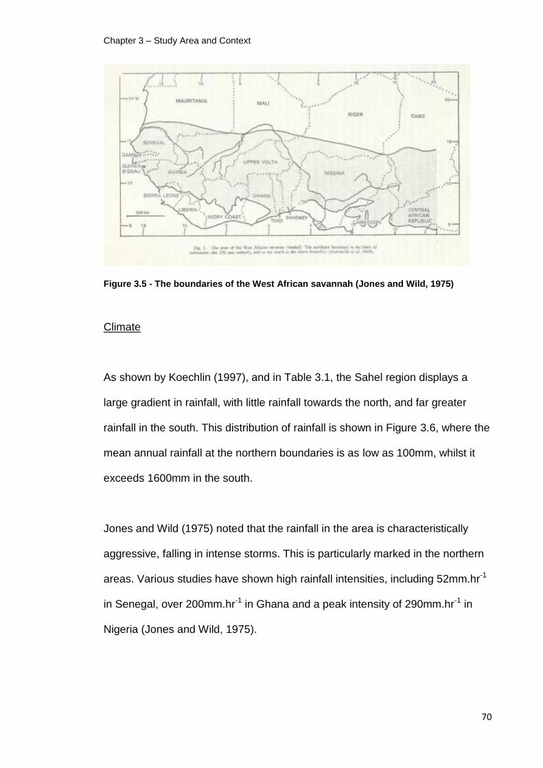
Chapter 3 – Study Area and Context
70
Figure 3.5 - The boundaries of the West African savannah (Jones and Wild, 1975)
Climate
As shown by Koechlin (1997), and in Table 3.1, the Sahel region displays a
large gradient in rainfall, with little rainfall towards the north, and far greater
rainfall in the south. This distribution of rainfall is shown in Figure 3.6, where the
mean annual rainfall at the northern boundaries is as low as 100mm, whilst it
exceeds 1600mm in the south.
Jones and Wild (1975) noted that the rainfall in the area is characteristically
aggressive, falling in intense storms. This is particularly marked in the northern
areas. Various studies have shown high rainfall intensities, including 52mm.hr-1
in Senegal, over 200mm.hr-1 in Ghana and a peak intensity of 290mm.hr-1 in
Nigeria (Jones and Wild, 1975).

Chapter 3 – Study Area and Context
71
Figure 3.6 - Isohyets of mean annual rainfall (mm) for the Western Sahel (after Jones and
Wild, 1975) – The Bakoye catchment is outlined in red and the Oualia gauging station is
highlighted by the green dot.
As well as the steep north-south gradient for mean annual rainfall, the same
gradient is evident in regards to the initiation and length of the wet season.
Figure 3.7 shows the gradient – for the Sahel region, the north has a short,
three month wet season beginning in July, and the south largely a 6 month wet
season, beginning in April (Jones and Wild, 1975).
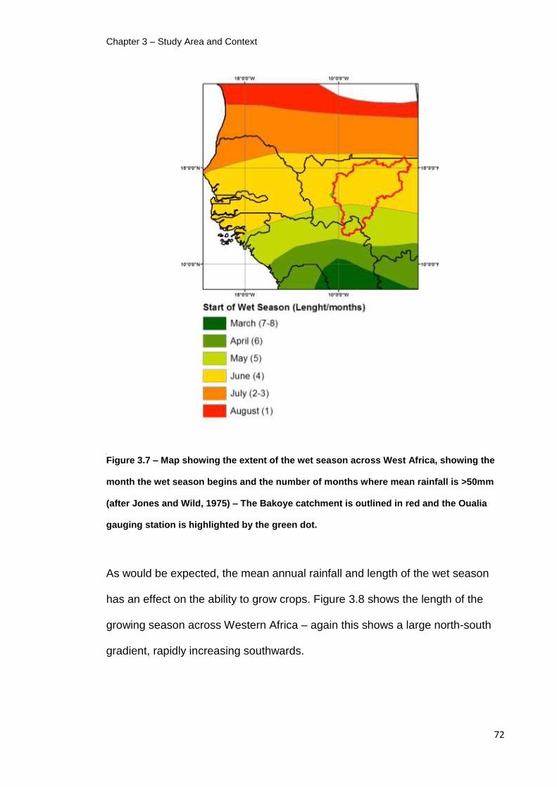
Chapter 3 – Study Area and Context
72
A
Figure 3.7 – Map showing the extent of the wet season across West Africa, showing the
month the wet season begins and the number of months where mean rainfall is >50mm
(after Jones and Wild, 1975) – The Bakoye catchment is outlined in red and the Oualia
gauging station is highlighted by the green dot.
As would be expected, the mean annual rainfall and length of the wet season
has an effect on the ability to grow crops. Figure 3.8 shows the length of the
growing season across Western Africa – again this shows a large north-south
gradient, rapidly increasing southwards.

Chapter 3 – Study Area and Context
73
Figure 3.8 - The length of the growing season, in days, across Western Africa (after
Jones and Wild, 1975) – The Bakoye catchment is outlined in red and the Oualia gauging
station is highlighted by the green dot.
The length of the growing season is linked to the relationship between potential
evapotranspiration (PET) and rainfall, where over the entire year in the Sahel
the PET exceeds the mean annual rain, but during the growing season the
rainfall is intense enough to create an excess (Jones and Wild, 1975).
Jones and Wild (1975) suggested that the Sahelian growing season can be
categorised into five distinct periods:

Chapter 3 – Study Area and Context
74
1. Preparatory period – rainfall is below PET but sufficient for cultivation
2. First intermediate period – rainfall close to PET, sufficient for sowing and
some growth
3. Humid period – rainfall exceeds PET
4. Second intermediate period – rainfall close to PET
5. Reserve period – PET exceeds rainfall, growth dependent on soil
moisture reserves
From north to south the humid period increases in length, along with the overall
growing season length, yet the other stages decrease in length (Jones and
Wild, 1975).
Similarly the influence of the climate has an input on the natural vegetation of
the region, and a generalised map of the vegetation zone across West Africa
can be seen in Figure 3.9.
It can be seen from the maps in Figure 3.6 to 3.9 that the Bakoye Catchment
straddles many climatic areas, in terms of mean annual rainfall, length of wet
season and vegetation zones. The majority of the catchment falls within the
area where the wet season can be expected to begin in June and last for four
months, and has a mean annual rainfall between 400-800mm. Vegetation is
varied across the catchment, with growing seasons lasting 80 days in the north,
and over 160 days in the south, and the catchment is almost equally divided
between the Northern Guinea, Sudan and Sahel vegetation zones.

Chapter 3 – Study Area and Context
75
Figure 3.9 – Map showing the generalised vegetation zones across West Africa (after
Jones and Wild, 1975) – The Bakoye catchment is outlined in red and the Oualia gauging
station is highlighted by the green dot. Northern Guinea – savannah. Sahel – wooded
steppe. Southern Guinea – relative moist undifferentiated savannah. Sudan – relatively
dry undifferentiated savannah.
Geology and Soil
Jones and Wild (1975) showed there to be a difference between the north and
the south in regards to rock types. The rocks of the south are dominated by

Chapter 3 – Study Area and Context
76
granites, and granite-derived metamorphic rocks, yet the north is largely
unconsolidated sands. Some areas in Mali, Senegal and Mauritania have large
areas of rocks associated with marine conditions, including conglomerates,
sandstones and clays. The lack of base-rich primary and volcanic rocks in the
region was highlighted.
Figure 3.10 - Generalised soil type distributions across the West African savannah (after
Jones and Wild, 1975) – The Bakoye catchment is outlined in red and the Oualia gauging
station is highlighted by the green dot.

Chapter 3 – Study Area and Context
77
Figure 3.10 shows the generalised soil type distributions across the region.
Jones and Wild (1975) suggested that the climate and vegetation have a
greater influence on the soil type than the parent material. The land surfaces
are predominantly from the late Cenozoic, with some older early Cenozoic
areas, with the soils having undergone several cycles of deposition and erosion,
resulting in the evidence of significant transportation and mixing. Younger
surfaces are restricted to the proximity of major rivers.
It can be seen in Figure 3.10 that the soil distributions broadly shows a north-
south gradient in the same way as the mean annual rainfall. Jones and Wild
(1975) saw this as a possible relationship, suggesting that the climate drives the
leaching and weathering rates, resulting in shallower soil profiles in the north.
The lack of vegetation towards the north also exposes the surface to heavier
erosion. In addition there is the potential for feedbacks from the land surfaces
that can define and/or reinforce the rainfall gradient in the Western Sahel
(Taylor and Lebel, 1998).
The Bakoye catchment itself shows significant heterogeneity of soil types
across its extent, with red/brown arid type soils in the north (corresponding with
the Sahel vegetation zone in Figure 3.9), tropical ferruginous soils in the south
and east, and weakly developed rocky soils in the west.

Chapter 3 – Study Area and Context
78
Topography
The Bakoye catchment also displays significant heterogeneity in topography
across its extent, as demonstrated in Figure 3.11 which shows the elevation
across West Africa as available from the National Geospatial-Intelligence
Agency (NGA, 2006).
Figure 3.11 – Map showing the topography of West Africa – The Bakoye catchment is
outlined in red and the Oualia gauging station is highlighted by the green dot (Elevation
data from NGA, cited 2006).
The elevation across the West African region can be seen to vary between
highlands in the south, largely within Guinea and Mali, with lowlands to the
north and west, particularly along the course of the River Senegal and the
Gambia where the elevation is almost wholly below 250m. The Bakoye

Chapter 3 – Study Area and Context
79
catchment shows significant variations, the south and east are mountainous
areas, and the height decreases towards the north. Most of the catchment is
above 250m elevation, but falls rapidly towards the outlet at the Oualia gauging
station.
Natural Hazards
The Sahel region is prone to drought and is often held as an example of the
dangers of environmental disaster, especially after the devastating drought that
persisted between 1968 and 1974 (Rain, 1999). Berry (1975) showed that
during this period, the Agades station in Niger recorded mean annual rainfalls
half the amount of the 50 year average between 1922 and 1972.
Similar droughts have occurred prior to the 1968-1974 event, such as in 1913
and 1940 (Berry, 1975). Balme et al. (2006) suggested that the Sahel region
had actually been in a state of drought from the late 1960s to the mid 1990s,
with intense peaks in 1972-1974 and 1983-1985. Most recently, the East
African Sahel was gripped by the Horn of Africa drought as described by
ADD12 and discussed in Section 3.2.
Overall the 1990-2002 rainfall for the Sahel was 20% below the 1950-1969
average, and 8% below the 1950-1989 average (Balme et al., 2006).
Although the region is prone to drought it is also prone to flooding. The risk of
flooding in West Africa is highlighted in Braman et al. (2012), showing that the

Chapter 3 – Study Area and Context
80
region is under increased risk because of development upon floodplains during
the long drought period, and the International Panel for Climate Change (IPCC)
predictions for more intense rainfall events for the region. In recent years there
has been an increase in flooding in the West African regions, as shown in
Figure 3.12
Figure 3.12 – Chart showing the increase in the number of annual floods in West Africa
between 1970-2008 (from Braman et al., 2012).
The Commission for Africa Report (Commission for Africa, 2010) highlighted the
expansion of deserts, or desertification, as a hazard facing the Sahel region.
Using a 3,200 year record of dust and proxy precipitation data from West Africa,
Mulitza et al. (2010) found that the relationship between Sahelian dust

Chapter 3 – Study Area and Context
81
generation and rainfall became decoupled around 1700AD, with the arrival of
commercial agriculture in the region, which may be contributing to the observed
desertification trend over the last four centuries.
Figure 3.13 – Chart showing the rainfall anomalies across the Sahelian zone (from
Conway, 2009).
The Sahelian region is currently in a multidecadal period of drought, which
began at the start of the 1970s (Conway, 2009) – this can be seen in the rainfall
anomaly chart in Figure 3.13. It is not certain whether this is due to natural
cycles – the area has experienced similar periods several times since the last
glacial period – or due to anthropogenic climate change (Conway, 2009).
The theory that desertification was occurring in the Sahel emerged from the
prolonged drought that afflicted the region after the 1960s, with the prevailing
thought being that mismanagement of the land had caused a climatic shift
(Giannini et al., 2008). Since the mid 1980s however, there was growing
evidence that the droughts were driven by changes in the global pattern of sea

Chapter 3 – Study Area and Context
82
surface temperatures (SST), and the rains have somewhat recovered with
‘greening’ evident in the region (Giannini et al., 2008).
With strong evidence for a link between warmer ocean temperatures and
Sahelian drought (Giannini et al., 2008), it stands to reason that with the
predictions for anthropogenic climate change that future warmer oceans will
lead to a drier Sahel, and desertification. However, Giannini et al. (2008)
suggested that recent observation and re-greening in the region contradict this
trend and theory, whilst Hein et al. (2011) noted that remote sensing techniques
have failed to detect wide-spread degradation of vegetation in the Sahel that
would be indicative of desertification.
The picture of desertification and possibilities for the future are unclear and
highly complex. Land degradation and farming plays a part in complex ways
(Conway, 2009), but the evidence points to a stronger link between droughts
and SST (Giannini et al., 2008). Conway (2009) shows that the main driver for
Sahelian droughts from SST is the difference in temperatures between the cool
North Atlantic and a warmer South Atlantic, but it appears that the South
Atlantic may have been cooling since the 1990s, and the North warming due to
climate change – this would lead to an increase of rainfall in the region.
3.4 – Previous Studies relating to the Bakoye Catchment
There have been five previous studies of the Bakoye Catchment that are
relevant to this study, details of which can be found in Hardy et al. (1989),

Chapter 3 – Study Area and Context
83
Andersen et al. (2002), Grimes and Diop (2003), Diop and Grimes (2003), and
Stisen et al. (2008). A summary of each is provided below –
Hardy et al. (1989)
The study described in Hardy et al. (1989) was one of the early applications of
the TAMSAT CCD method to drive a manually calibrated Pitman lumped CRR
model of the Manantali and Gourbassy catchments, upstream sub-catchments
of the Senegal Basin.
The study found that the Pitman model performed comparatively well compared
to the model driven by raingauge data, with the benefit of being produced in
near real-time. The study acknowledged the requirement for further research,
including on other catchments but also acknowledged the implications of
hydrological model calibration when using the SRFE.
Andersen et al. (2002)
Andersen et al. (2001) described the calibration and validation of a MIKE SHE
distributed and physically based hydrological model of the Senegal Basin. The
same model was used but with remotely sensed data to drive it in Andersen et
al. (2002), including a TAMSAT CCD estimate of rainfall to fill in areas that were
more than 25km away from a recording raingauge station. The study found that
the use of the TAMSAT rainfall did not improve the performance of the overall
model but there was some improvement at smaller scales, which could be

Chapter 3 – Study Area and Context
84
further improved as the additional spatial information provided by TAMSAT
estimates would allow a higher resolution to be used for future modelling.
Grimes and Diop (2003)
The study described in Grimes and Diop (2003) compared the performance of
TAMSAT estimates to inputs from a NWP model incorporating satellite data and
a mean of the raingauges within the catchment, when used to drive a pre-
calibrated Pitman lumped CRR model. Included as part of this study was a
modelling of storm types and the influence of the African Eastern Waves
(AEWs). The study found that a NWP model utilising satellite data, with a
contemporaneous calibration can outperform raingauge data alone for driving a
hydrological model, and this can be further improved by including information on
storm types and wave phases.
In addition the study also found that inclusion of a relatively complex modelling
of PET in the Pitman model - using remotely sensed NDVI data - did not
improve the modelling of the catchment.
Diop and Grimes (2003)
The study described by Diop and Grimes (2003), a companion paper to Grimes
and Diop (2003) summarised above, investigated the influence of the AEWs on
the Bakoye Catchment, and the modelling of rainfall and hydrology.

Chapter 3 – Study Area and Context
85
Produced by instabilities in the African Easterly Jet, AEWs form and travel
westwards over North Africa, into the Atlantic and are linked to the formation of
tropical cyclones there. For the region of the Senegal Basin and the Bakoye
catchment they are significant in that they are key drivers of convection, and the
rainfall that results. The study found that the highest levels of rainfall and CCD
occurred on the leading edge of the waves, with minima in the trough behind,
however the relationship was complex and showed significant inter-annual
variation indicating the influence of other meteorological factors. As stated
above, Grimes and Diop (2003) showed that the inclusion of wave phase and
storm type classification in the modelling process improved performance.
Stisen et al. (2008)
The study described by Stisen et al. (2008) looked at using remote sensing data
to drive a MIKE SHE distributed hydrological model of the Senegal Basin,
including six sub-catchments, one of which being the Bakoye catchment.
Rainfall data for the study was produced using TAMSAT CCD estimates.
The study concluded that remotely sensed data could provide a valid means of
driving a distributed hydrological model for a large river basin, and that by
comparing data for a single sub-catchment and previous studies, a distributed
approach outperformed less sophisticated lumped methods, especially in the
robustness of the calibration.

Chapter 3 – Study Area and Context
86
The Current Picture
It would appear from the studies above that the picture of using SRFE to drive a
hydrological model for the Bakoye Catchment is mixed. Hardy et al. (1989) and
Grimes and Diop (2003) both showed that TAMSAT rainfall estimates can be
used effectively to drive a lumped hydrological model of a sub-catchment of the
Senegal Basin, and Stisen et al. (2008) demonstrated that TAMSAT could also
be used effectively with a distributed model of the larger basin area. However,
Andersen et al. (2002) suggested that the TAMSAT rainfall did not improve the
performance of the model at the catchment level.
Diop and Grimes (2003) showed that by introducing the modelling of storm type
and wave phases to the modelling of rainfall from satellite data, the
performance when driving a lumped model was improved. None of the previous
studies have attempted to model the uncertainty within the SRFE and how it
influences and propagates through the hydrological model.
3.5 – The Available Data
This section will examine the datasets that have been made available to this
thesis, plus the additional sources of data to supplement it. The section will also
investigate the data in relation to the climatic conditions discussed earlier in this
chapter. The main sources of data available were:
Historic Raingauge Data

Chapter 3 – Study Area and Context
87
Historic Discharge Data
Historic Satellite Data
Additional sources of data available which have been used are:
Climatic Potential Evaporation Data
Digital Elevation Model Data
The Raingauge Data
Data from 81 raingauge stations are available, recording the period between
1986 and 1996, at a daily timestep. Figure 3.14 shows the locations of each of
the raingauges available, and their percentage of recording coverage between
1986 and 1996.
Coverage of the raingauges is generally good, with an all-over average of
77.71%. 22 stations have data recorded for 100% of the period, 48 stations
have over 75% and 67 stations have at least 50% coverage. Only 4 stations
record data for less than 25% of the period. Ideally, stations that show such a
poor record of coverage would be excluded from the dataset, but due to the
already sparse nature of the data all stations were included.

Chapter 3 – Study Area and Context
88
Figure 3.14 – Map showing the extent of the study area and location of the 81 raingauge
stations. The percentage of recording coverage provided by each station is shown for
the period between 1986 and 1996, with green stars indicating those stations that provide
100% coverage. The extent of the Bakoye catchment is outlined in red.
Table 3.2 shows the mean annual rainfall for each year of the study taken from
all 81 stations, with each station having been weighted depending on the
number of days it has recorded data that year. The table also shows the
average coverage for each year.

Chapter 3 – Study Area and Context
89
Year Weighted Mean
Rainfall (mm.yr-1) Coverage (%)
1986 592.95 88.44
1987 580.63 84.93
1988 689.89 80.13
1989 686.37 76.66
1990 528.82 73.73
1991 549.60 76.86
1992 503.41 68.51
1993 521.41 71.81
1994 715.75 79.61
1995 681.77 78.38
1996 635.54 75.70
Total 6686.14
Mean 607.83 77.71
Table 3.2 – Mean annual rainfall for each year taken from all the 81 raingauge stations for
the period between 1986 and 1996, and the mean recording coverage of the stations for
that period.
Figure 3.15 – Chart showing the deviation from the 1986-1996 rainfall mean for each year
of the study period, for all the raingauge stations.
-150.00
-100.00
-50.00
0.00
50.00
100.00
150.00
1986 1987 1988 1989 1990 1991 1992 1993 1994 1995 1996
Rai
nfa
ll B
alan
ce f
rom
me
an (
mm
.yr-
1)
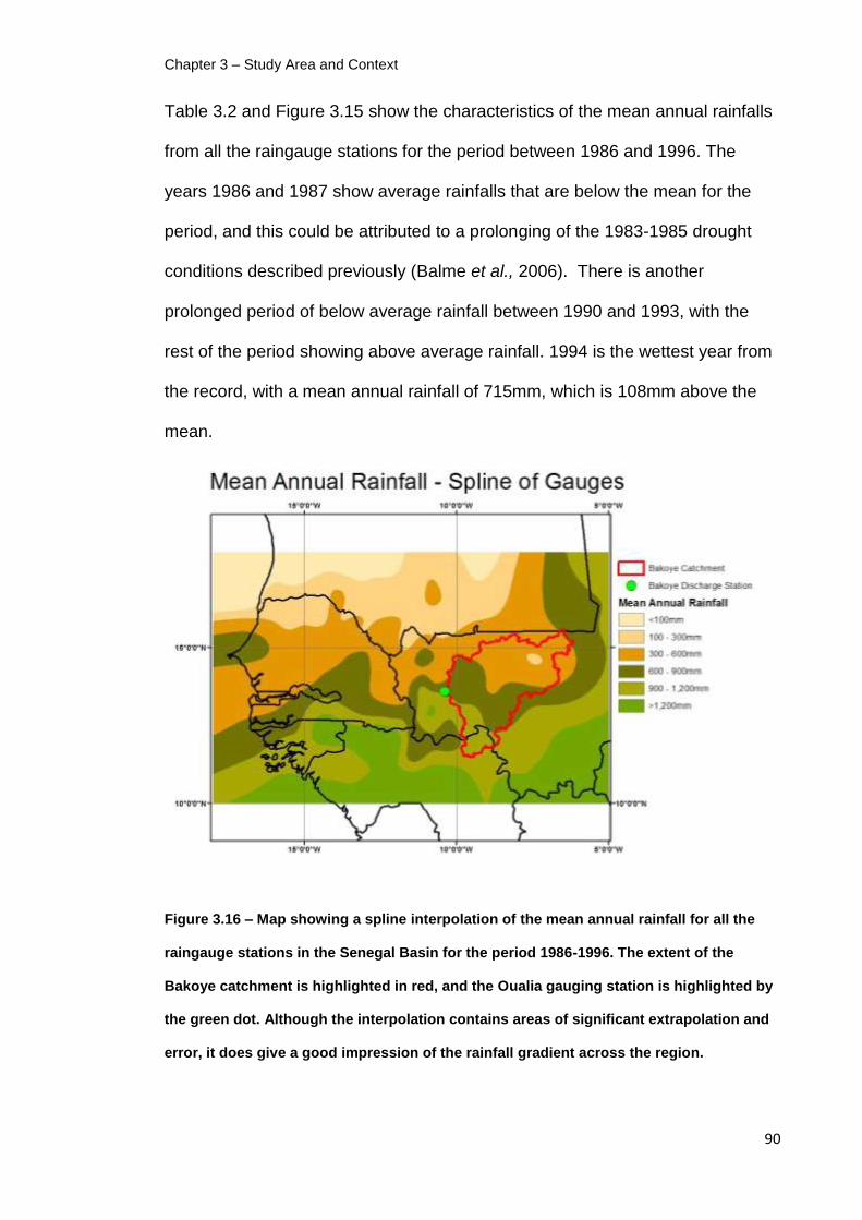
Chapter 3 – Study Area and Context
90
Table 3.2 and Figure 3.15 show the characteristics of the mean annual rainfalls
from all the raingauge stations for the period between 1986 and 1996. The
years 1986 and 1987 show average rainfalls that are below the mean for the
period, and this could be attributed to a prolonging of the 1983-1985 drought
conditions described previously (Balme et al., 2006). There is another
prolonged period of below average rainfall between 1990 and 1993, with the
rest of the period showing above average rainfall. 1994 is the wettest year from
the record, with a mean annual rainfall of 715mm, which is 108mm above the
mean.
Figure 3.16 – Map showing a spline interpolation of the mean annual rainfall for all the
raingauge stations in the Senegal Basin for the period 1986-1996. The extent of the
Bakoye catchment is highlighted in red, and the Oualia gauging station is highlighted by
the green dot. Although the interpolation contains areas of significant extrapolation and
error, it does give a good impression of the rainfall gradient across the region.

Chapter 3 – Study Area and Context
91
Figure 3.16 shows a spline plot of the mean annual rainfall from the gauges
across the Senegal Basin area. The mean annual rainfall region (607mm) lies
between the dark-brown and dark-green bands.
There are 13 raingauge stations from the record that can be said to be
associated with the Bakoye Catchment. These 13 stations will form a sub-set
for use in determining the seasonal variations of rainfall over the Bakoye
catchment. The mean annual rainfalls for the study period, determined from
these stations, are shown in Table 3.3, along with the average recording
coverage.
Year Weighted Mean Rainfall
(mm/yr) Coverage (%)
1986 772.59 100.00
1987 621.84 99.98
1988 892.78 69.23
1989 848.17 76.92
1990 694.74 76.92
1991 760.27 76.92
1992 660.88 59.58
1993 723.25 58.29
1994 940.01 74.35
1995 814.75 75.01
1996 768.36 62.82
Total 8497.64
Mean 772.51 75.46
Table 3.3 – Mean annual rainfall for each year taken from all the Bakoye catchment sub-
set of raingauge stations for the period between 1986 and 1996, and the mean recording
coverage of the stations for that period.

Chapter 3 – Study Area and Context
92
Figure 3.17 – Chart showing the deviation from the 1986-1996 rainfall mean for each year
of the study period, for the Bakoye catchment sub-set of raingauge stations.
Table 3.3 and Figure 3.17 show the characteristics of the mean annual rainfall
for the Bakoye catchment, based on a sub-set of 13 raingauge stations. The
general pattern is similar to that of the wider Senegal Basin, with dry periods
between 1986-87 and 1990-93, with 1994 being the wettest year. However, the
rainfall in 1986 is slightly more than the mean for the period, and 1996 slightly
below – a deviation from the pattern seen for the whole of the Senegal Basin.
Overall the catchment has a higher mean annual rainfall than the Senegal Basin
as a whole, which is expected as the Bakoye catchment predominantly lies
towards the climatologically wetter, southern end of the Basin. This can been
seen in Figure 3.16, with significant areas of the catchment covered by bands of
rainfall above the mean annual rainfall for the Senegal Basin (607mm).
However, this might be skewed because the wetter regions of the Bakoye

Chapter 3 – Study Area and Context
93
catchment are more densely gauged than the drier northern areas, which lie in
areas of mean annual rainfall below the overall mean, likely to result in
overestimation of rainfall for the catchment from the gauges here.
The River Discharge Data
The available river discharge data is from seven discharge stations, with various
periods of coverage between 1986 and 2005.
Figure 3.18 – Map showing the locations of the river discharge stations of the Senegal
Basin and the associated catchment extents. The Oualia station records the output from
the Bakoye catchment. The numbers show the percentage of discharge for each
catchment in relation to discharge of the Bakel station (for 1998-2001) (from Stisen et al.,
2008).

Chapter 3 – Study Area and Context
94
Figure 3.18 shows the locations of the discharge stations and their associated
upstream catchments. From 1987 the discharge from the Manantali outlet is
controlled by the dam located there, and the discharge data shows little
correlation with rainfall calculated from raingauges within its catchment. As the
discharge from Manantali accounts for 43% of that recorded by the Bakel
station (Stisen et al., 2008), it would be expected that the output from the dam
would have significant impact on the discharge downstream, and this is
reflected in the data for Kayes and Bakel.
The sub-catchments of Mankana and Dakka, upstream of Manantali, do not
cover enough area to be represented by a sub-set of raingauges, so the
influence of the dam at Manantali cannot be assessed, but it is anticipated to be
significant.
Of the catchments, the Gourbassa and Bakoye catchments are the best suited
for modelling, both being free from the influence of the Manantali dam. Both
have a similar output, 20% of the Bakel discharge for Gourbassa, and 18% in
the case of Bakoye, yet the Gourbassa catchment is the smaller. This is an
issue, as there are five raingauge stations that can be associated with the
Gourbassa Catchment (with periods of only two stations recording), and 13
associated with the Bakoye Catchment – this makes the Bakoye catchment the
most suitable catchment to model.
Although data is available for the period 1986-2005 for the Oualia station which
sits at the outlet of the Bakoye Catchment, raingauge data is only available for

Chapter 3 – Study Area and Context
95
the period 1986-1996. Figures 3.19 and 3.20 show the characteristics of the
mean annual discharge for the Bakel and Oualia stations respectively.
Figure 3.19 – Chart showing deviation of mean annual discharge for the Bakel station
from the mean annual discharge for the period 1986-1996.
Figure 3.20 – Chart showing deviation of mean annual discharge for the Oualia station
from the mean annual discharge for the period 1986-1996.

Chapter 3 – Study Area and Context
96
The patterns shown in Figures 3.19 and 3.20, in the main, resemble the
variations from mean annual rainfall shown both for the Senegal Basin area in
Figure 3.15, and the Bakoye catchment in Figure 3.17. There are dry periods in
1986-87 and 1990-93, and the discharges for 1994 reflect the fact that the
raingauge stations indicated that it was the wettest year of the record. However,
1989, which is a relatively wet year according to the raingauge stations shows
below average discharge.
Interestingly, 1996 displayed below average rainfall over the Bakoye catchment
yet above average discharge. It is clear that the relationship between a simple
average of raingauge measurements and catchment discharge is likely to be
non-linear, non-stationary (both temporally and spatially) and uncertain at best.
In absence of a more accurate alternative, the raingauge and discharge station
data will be assumed to be free of error and uncertainty, although this is clearly
not the case.
Satellite Data
The third important dataset available to the study was the satellite data, in the
form of ‘Cold Cloud Duration’ (CCD) data, produced by the Tropical Applications
of Meteorology using SATellites (TAMSAT) research group, Department of
Meteorology, University of Reading.
The CCD method employed by the TAMSAT group utilises the 10-13μm infra-
red channel of the Meteosat satellites to capture cloud top temperatures at

Chapter 3 – Study Area and Context
97
quarter-hourly intervals. For each 0.05° pixel a value is produced for the amount
of time that pixel records temperatures below specified thresholds for each day.
That value is the pixel’s daily CCD value.
The database provided includes data for the whole of sub-Saharan Africa for
the period of 1983-2010, at daily timesteps at a resolution of 0.05°. It is provided
for the temperature thresholds of -20°c, -30°c, -40°c, -50°c and -60°c.
Seasonality in the Data
There is a large seasonality displayed across the region, as described by Jones
and Wild (1975), with much of the Senegal Basin area within the region where
the wet season can be expected to begin in June and last for four months.
The seasonality expected is seen in the data, as shown in Figure 3.21. The vast
majority of the rainfall falls between June and September, with peak rainfalls in
August which accounts for 31% of the annual rainfall. The period between June
and September accounts for 88% of the annual rainfall. There are still
reasonably significant rainfalls in May and October, but these are still only 4%
and 7% of the annual total.
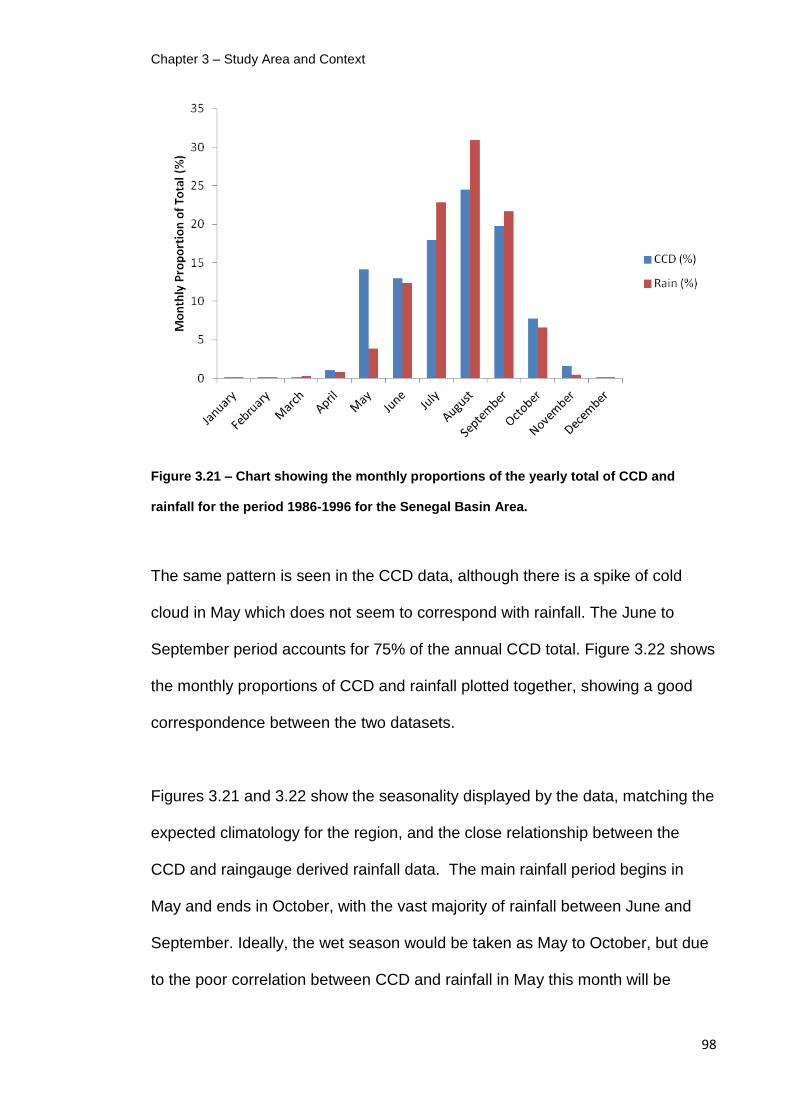
Chapter 3 – Study Area and Context
98
Figure 3.21 – Chart showing the monthly proportions of the yearly total of CCD and
rainfall for the period 1986-1996 for the Senegal Basin Area.
The same pattern is seen in the CCD data, although there is a spike of cold
cloud in May which does not seem to correspond with rainfall. The June to
September period accounts for 75% of the annual CCD total. Figure 3.22 shows
the monthly proportions of CCD and rainfall plotted together, showing a good
correspondence between the two datasets.
Figures 3.21 and 3.22 show the seasonality displayed by the data, matching the
expected climatology for the region, and the close relationship between the
CCD and raingauge derived rainfall data. The main rainfall period begins in
May and ends in October, with the vast majority of rainfall between June and
September. Ideally, the wet season would be taken as May to October, but due
to the poor correlation between CCD and rainfall in May this month will be

Chapter 3 – Study Area and Context
99
excluded. Still, the defined wet season of June to October accounts for 95% of
the rainfall recorded by the raingauge stations.
Figure 3.22 – Scatter plot showing the relationship between the monthly CCD and rainfall
proportions of the annual total for the period 1986-1996 for the Senegal Basin area.
Climatic Potential Evapotranspiration Data
In a similar way to ground instrumentation for rainfall, the Senegal Basin area
does not contain the infrastructure for recording evapotranspiration rates at high
spatial or temporal resolution. For use in this thesis, monthly climatic derived
values are used, taken from the Food and Agriculture Organisation of the
United Nations (FAO), available from FAO (2009) – the values used are from
the nearest point available to the Oualia gauging station.
The climatic monthly averages of reference evapotranspiration are determined
by the FAO (2009), using the Montieth-Penman method, which is outlined in

Chapter 3 – Study Area and Context
100
Allen at al (1998). In a review of different methods of evaluating climatic
evapotranspiration data, the CGIAR-CSI (2009) found that the Montieth-
Penman method outperformed the others, the details of which can be seen in
Figure 3.23. These findings were similar to Batchelor (1984) which
demonstrated that the method was superior in most practical situations. As can
be seen in Figure 3.23, the Montieth-Penman does not have the spatial
resolution of the other methods but as a lumped value was used this is not
relevant. The Montieth-Penman has the additional benefit of being available for
download without the need for additional processing.
The Montieth-Penman method makes assumptions that could be a source of
uncertainty in hydrological modelling. As a climatic representation of
evapotranspiration it lacks the temporal resolution of the model, and cannot
account for annual variations from the climatic average. It is also unable to
account for antecedent conditions, which Taylor and Lebel (1998) suggested
could be significant on the amount of soil moisture, evapotranspiration and
feedbacks to rainfall amount. The Montieth-Penman method makes the
assumption of global homogeneity in crop types, described as being 0.12m in
height, with a surface resistance of 70s.m-1 and an albedo of 0.23 (Allen et al.,
1998) – obviously this assumption is incorrect and the heterogeneity of
vegetation has been shown across the Bakoye catchment in Figures 3.8 and
3.9.

Chapter 3 – Study Area and Context
101
Figure 3.23 – Comparison of methodologies for producing reference climatic
evapotranspiration data (from CGIAR-CSI, 2009).
Some attempts can be made to mitigate these issues, such as smoothing the
data into dekadal time steps, but this is unlikely to significantly improve the
quality of the data. Remote sensing has been used to improve the spatial and
temporal resolution of evapotranspiration data, and Courault et al. (2005)
provided an overview of the techniques, broadly categorising them into four
types:
1. Direct empirical methods, for example those based on TIR images
2. Residual methods of the energy budget using remotely sensed data with
physical parameters
3. Deterministic models such as Soil-Vegetation-Atmosphere-Transfer
(SVAT)

Chapter 3 – Study Area and Context
102
4. Vegetation index methods used as adjustments to the initial data
Stisen et al. (2008) attempted to improve the temporal resolution of remotely
sensed evapotranspiration values by modifying them with satellite derived
Normally Distributed Vegetation Index (NDVI) data – the NDVI data was
available at daily time steps with a spatial resolution of 6km, and was used as
an indicator of Leaf Area Index (LAI). The approach by Stisen et al. (2008) was
similar to that used by Grimes and Diop (2003) which incorporated daily NDVI
data to adjust the FAO climatic estimates, finding no improvement to the model.
Baret and Guyot (1991) found that NDVI was highly sensitive to soil optical
properties, particularly in areas of low vegetation, showing that other methods
outperformed NDVI – it is possible that the approach by Grimes and Diop
(2003) was correct but the NDVI data used was not suitable for the Bakoye
catchment.
Courault et al. (2005) suggested that the methods of perturbing climatic
estimates based on remotely sensed data were unlikely to estimate the spatial
and temporal variations of evapotranspiration with a high degree of accuracy.
Despite this and although Grimes and Diop (2003) found that a more
sophisticated method of incorporating PET into the model did not improve
performance – and indeed initial tests performed for this thesis found similar
results – their use of such methods cannot be excluded from future research
and disregarded, especially with the use of a distributed hydrological model and
more research is required in this area.

Chapter 3 – Study Area and Context
103
Digital Elevation Data
The digital elevation data used for the thesis is taken from the National
Geospatial-Intelligence Agency (NGA, 2006). The elevation data for West Africa
can be seen earlier in this Chapter in Figure 3.11.
3.6 – Summary
This chapter has demonstrated how the Sahel region is an area that faces
many problems, from food insecurity, drought and famine, to flooding and
desertification due to climate change, amongst others. Many agencies have
attempted to assist the area’s development and help to mitigate and limit the
impacts of disasters if they do occur.
A key component to the success of these efforts are the environmental models
that are used to inform EWS, but these rely on timely and accurate
measurements of precipitations which, when compared to other areas of the
globe, are scarce. SRFE have been shown to improve the spatial and temporal
resolution of the precipitation data available to environmental models in the
Sahel but these can be highly uncertain, and there is a requirement to
accurately measure this uncertainty, characterise it in a way that is applicable to
an environmental model, and clearly communicate it in a way that can be
understood by decision makers.

Chapter 3 – Study Area and Context
104
The Senegal Basin and the Bakoye catchment within it are typical of the Sahel
region, and pose a challenge for producing SRFE. The precipitation data from
ground recording instrumentation is particularly sparse, and the region displays
significant heterogeneity in terms of climate, land cover and geology. This
makes the need for accurate uncertainty characterisation even more urgent for
SRFE in this area.
The following three chapters detail the methodology adopted for this thesis.
Chapter 4 demonstrates how the point raingauge network was interpolated into
a continuous grid. Chapter 5 describes the TAMSAT1 method of producing a
deterministic SRFE, and the TAMSIM algorithm for characterising the
uncertainty using a fully spatio-temporally distributed stochastic ensemble
method. Chapter 6 demonstrates the Pitman lumped CRR model used for the
hydrological modelling part of the thesis, and the SCE-UA technique used to
optimise the variable parameters.

Chapter 4 – Methodology – Spatial Interpolation
105
4 Methodology – Spatial Interpolation
4.1 – Introduction
This chapter is the first of three methodology chapters and details the methods
used in the spatial interpolation of the point raingauge data. This is a necessity
in order to make the data directly compatible and comparable to the satellite
data which is aggregated at 0.5º pixels. The method chosen to perform the
spatial interpolation was the double Kriging (DK) method introduced by
Barancourt et al. (1992).
4.2 – Spatial Interpolation and the Double Kriging (DK) Method
In order to calibrate the satellite data using historical raingauge data one of two
approaches must be taken – either calculate point values from the satellite pixel
averages, or produce pixel averages of the raingauge data (Grimes et al.,
1999). For this thesis, the latter approach has been adopted and therefore it is
necessary to produce daily average rainfalls for the Senegal Basin at an
appropriate pixel size, and the DK method of Barancourt et al. (1992) has been
chosen to compute the pixel averages from the raingauge data.

Chapter 4 – Methodology – Spatial Interpolation
106
Kriging is a linear interpolation method common to geostatistics, although it has
been used widely across many and varied disciplines, for example estimating
the proportion of shading across large photovoltaic cells (Di Piazza and Di
Piazza, 2009) and even graphical character animation (Courty and Cuzol,
2010), which highlights its versatility.
Kriging is a popular approach for the spatial interpolation of rainfall fields and its
usefulness has been demonstrated for a variety of applications, including
hydrological modelling (Sun et al., 2000), climate studies (Duchon et al., 1995;
Pardo-Iguzquiza, 1998), pollution modelling (Shen et al., 2012), producing
large, gridded datasets (Jeffrey et al., 2001; Haylock et al., 2008; Hofstra et al.,
2009), designing raingauge networks (Pardo-Iguzquiza, 1998; Campling et al.,
2001), producing reference fields for error characterisation (Kirstetter et al.,
2010) and calibration of remote sensing techniques (Grimes et al., 1999). It has
been found to outperform other methods for spatial interpolation of rainfall,
including inverse-distance (Dirks et al., 1998), Theissen Polygon (Dirks et al.,
1998; Goovaerts, 2000) and multi-quadratic interpolation (Syed et al., 2003) –
although Dirks et al. (1998) and Syed et al. (2003) both suggest that for small
catchments with a dense network, the benefits of Kriging are negligible
compared to simple methods especially when considering the additional
computational expense. Dirks et al. (1998) added that the benefits of Kriging are
more fully realised when the study was sufficiently large to exploit the full extent
of the semi-variogram.

Chapter 4 – Methodology – Spatial Interpolation
107
Kriging is not without its limitations and Hofstra et al. (2009), on spatial
interpolation in general, suggested that the network density, spatial
characteristics of the variable and the complexity of the terrain all have an effect
on the accuracy of the interpolation.
With Kriging there is a tendency for interpolated values to converge upon the
mean, described in Haylock et al. (2008) as a smoothing of extreme events,
where the Kriging interpolation was found to be smoothing the peaks and
troughs of the gauge data. Maidment et al. (in press 2012) also observed this
effect with block Kriging but suggested that in this case it is likely to be
physically correct, with high values representing a ‘direct hit’ over the gauge
when rainfall elsewhere in the pixel is lower, and vice versa. Only by
experimental testing could this be proven or otherwise, and this would require a
dense network of gauges at sub-pixel level (Maidment et al., in press 2012).
In the pursuit of more realistic realisations of precipitation fields, several
variations of the Kriging methodology have been developed. Goovaerts (2000)
explored some of these methods for incorporating secondary information, in this
case elevation data in the form of a DEM, into the algorithm. The techniques
were linear regression, simple Kriging (SK) with linear mean, Kriging with
external drift and ordinary Kriging (OK), and it was found that the algorithms
incorporating the secondary information outperformed OK (Goovaerts, 2000).
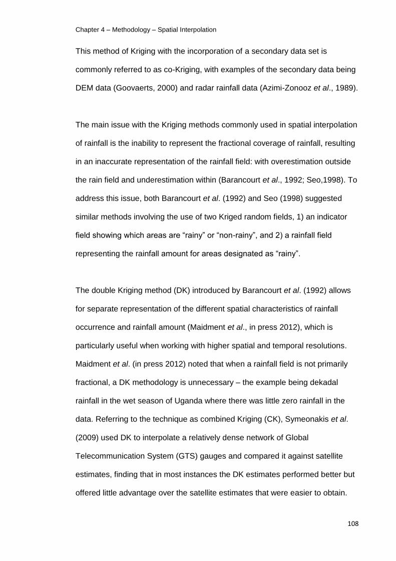
Chapter 4 – Methodology – Spatial Interpolation
108
This method of Kriging with the incorporation of a secondary data set is
commonly referred to as co-Kriging, with examples of the secondary data being
DEM data (Goovaerts, 2000) and radar rainfall data (Azimi-Zonooz et al., 1989).
The main issue with the Kriging methods commonly used in spatial interpolation
of rainfall is the inability to represent the fractional coverage of rainfall, resulting
in an inaccurate representation of the rainfall field: with overestimation outside
the rain field and underestimation within (Barancourt et al., 1992; Seo,1998). To
address this issue, both Barancourt et al. (1992) and Seo (1998) suggested
similar methods involving the use of two Kriged random fields, 1) an indicator
field showing which areas are “rainy” or “non-rainy”, and 2) a rainfall field
representing the rainfall amount for areas designated as “rainy”.
The double Kriging method (DK) introduced by Barancourt et al. (1992) allows
for separate representation of the different spatial characteristics of rainfall
occurrence and rainfall amount (Maidment et al., in press 2012), which is
particularly useful when working with higher spatial and temporal resolutions.
Maidment et al. (in press 2012) noted that when a rainfall field is not primarily
fractional, a DK methodology is unnecessary – the example being dekadal
rainfall in the wet season of Uganda where there was little zero rainfall in the
data. Referring to the technique as combined Kriging (CK), Symeonakis et al.
(2009) used DK to interpolate a relatively dense network of Global
Telecommunication System (GTS) gauges and compared it against satellite
estimates, finding that in most instances the DK estimates performed better but
offered little advantage over the satellite estimates that were easier to obtain.

Chapter 4 – Methodology – Spatial Interpolation
109
Teo (2006) used a cross-validation method, sequentially removing a single
raingauge point from the Kriging method for each timestep, to assess the
capabilities of both DK and OK for determining point estimates. Using numerous
skill measures, the DK method outperformed OK, the latter was found to reduce
the heterogeneity of intermittent rainfall fields.
The Double Kriging (DK) Method
The DK method was first described in Barancourt et al. (1992). For this thesis
the KrigeRain algorithm (Greatrex, 2009) was used to conduct the DK on the
raingauge data from the study area, and this section provides a summary of the
DK method and the functionality of the KrigeRain algorithm. The description of
the method in Teo (2006) should be seen for a full methodology and
background.
The DK method involves the production and combination of two random fields
(RF) which together produce a fractional mean areal rainfall field. The two RFs
required are –
1. a binary ‘indicator’ rain/no-rain field of thresholded rainfall probabilities -
.
2. a ‘no-zero rainfall’ field showing the variability of rainfall with the zero
values removed - .

Chapter 4 – Methodology – Spatial Interpolation
110
Equation 4.1
Equation 4.1 shows the combination of the two RFs outlined above, where is
the DK product of the two RFs and is a pixel location. The remainder of this
section is divided into first summarising the generation of the Indicator ( ) field,
and then summarising the generation of the no-zero rainfall ( ) field.
Generation of , the Indicator Field
In order to produce daily fractional mean areal rainfall field it is necessary to
determine which areas are likely to be raining, and which are not. In the DK
method of Barancourt et al. (1992) this was achieved by using a binary
indicator, rain/no-rain, RF of thresholded rainfall probabilities.
Equation 4.2
The production of the binary field is shown in Equation 4.2. is the
probability of rainfall at pixel , produced by OK of the binary rainfall state of the
raingauges. represents the probability threshold which is determined for each
day so that the resulting field will produce the same proportion of raining pixels
as the proportion of raingauges recording rain for that day. If the probability of
rainfall for a pixel is above the threshold it is assigned a rainy status, 1, and if it
is below it is assigned a non-rainy status, 0.

Chapter 4 – Methodology – Spatial Interpolation
111
Generation of , the ‘No-Zero Rainfall’ Field
With the indicator field representing the areas that are likely to be raining or not
raining, it is then necessary to produce a rainfall field showing the rainfall
volumes at each pixel. The resulting field needs to produce a total volume of
rainfall across the field that is in line with the total volume of rainfall suggested
by the raw raingauge data. The DK method described of Barancourt et al.
(1992) used a ‘no-zero rainfall’ method to produce this field.
The ‘no-zero rainfall’ field, , is produced by OK of the raingauge data only for
raingauges that record positive rainfall, for each day, for the entire study area.
The resulting rainfall field obviously shows much greater rainfall volumes than
an OK produced rain field from all of the raingauge data, but when combined
with the ‘indicator’ field the total volume is reduced to a more representative
amount.
4.3 – Implementation of the DK Method
4.3.1 – Introduction
This section details the implementation specifics for the double Kriging (DK)
method for the spatial interpolation of the daily rain field for the Senegal Basin.
4.3.2 shows the calibration using the historic raingauge data, and 4.3.3 part

Chapter 4 – Methodology – Spatial Interpolation
112
demonstrates how DK daily rain field relates to the original gauge data. This
section concludes in 4.3.4.
4.3.2 – Calibration
The daily raingauge data covering the Senegal Basin area, for 1986 to 1996,
was spatially interpolated using the DK method detailed above. The process
was performed using the KrigeRain V1.1 algorithm for the R environment
(Greatrex, 2009).
Chapter 3 looked at the raw raingauge data and showed that the likelihood of
rain and the rainfall amount was heterogeneous over the region, and because
of this it is impossible to represent the true nature of the rain field statistics with
a stationary and ergodic rain field. Goovaerts (2000) showed how secondary
information, incorporated into the Kriging process, can be an effective way of
producing a non-stationary, non-ergodic underlying rain field, but with the
paucity of raingauges available it is unlikely that sufficient detail would be
available to fully represent the heterogeneity. However, considering the above
limitations, it is reasonable to compromise and treat the spatial characteristics of
rainfall occurrence and amount as stationary and ergodic – represented by
climatological variograms.
The ideal situation would be the generation of variograms that describe each
individual storm event, but in reality it is unusual for sufficient data to be
available to do this and climatological variograms are a reasonable alternative

Chapter 4 – Methodology – Spatial Interpolation
113
(Grimes and Pardo-Iguzquiza, 2010). With data used in this thesis there was
not enough sufficient coverage, and/or enough positive rainfall in the record to
produce climatological variograms for each month, so a wet season variogram
was used instead. There was insufficient positive rainfall to produce a dry
season variogram.
Figures 4.1 and 4.2 show the standardised experimental variograms and the
fitted climatological variograms for the wet season. In comparison to other
studies, the nugget effect in the indicator variogram is relatively modest – Teo
(2006) produced nuggets of 70-80% of the sill, suggesting that this showed
intermittencies at a scale smaller than the gauge network could detail. The
nugget effect here of 37% could suggest that such intermittencies are less
prevalent for this region, but could be a result of the bin size selected.
The climatological variograms were generated after experimental variograms
were produced, and the parameters adjusted to produce a suitable modelled
variogram. Figures 4.3 and 4.4 shows an example of experimental variograms -
demonstrating the selection of a suitable binsize. The binsize was required to
be narrow enough to reflect the relationship over distance, yet not be so narrow
that the relationship becomes noisy. For both the no-zero and indicator
variograms a binsize of 25km was selected.

Chapter 4 – Methodology – Spatial Interpolation
114
Figure 4.1 – Wet season climatological Indicator variogram for the daily Senegal Basin
rainfall field. Range is defined as the distance where the semivariance is 95% of the sill.
Figure 4.2 - Wet season climatological no-zero rainfall variogram for the daily Senegal
Basin rainfall field. Range is defined as the distance where the semivariance is 95% of
the sill.
Chapter 4 – Methodology – Spatial Interpolation
115
The experimental variograms shown in Figures 4.3 and 4.4 were also used to
set the maximum extent of the variograms, this being the distance where the
relationship begins to degrade and becomes noisy. Figures 4.5 and 4.6 are
plots showing the number of station pairs over distance, which were also used
in the selection of a maximum extent distance – the maximum distance should
be set before the number of pairs becomes too low. For both the no-zero and
indicator variograms, this maximum extent was set at 600km. Although at that
distance both fields retain a reasonable number of station pairs, it is at this
distance where the variograms clearly start to degrade.
Figure 4.3 – Experimental ‘no-zero’ variograms generated by KrigeRain using different
binsize settings.

Chapter 4 – Methodology – Spatial Interpolation
116
Figure 4.4 – Experimental ‘indicator’ variograms generated by KrigeRain using different
binsize settings.

Chapter 4 – Methodology – Spatial Interpolation
117
Figure 4.5 – Chart showing number of station pairs at distance for ‘no-zero’ rain field.
Figure 4.6 – Chart showing number of station pairs at distance for ‘indicator’ rain field.
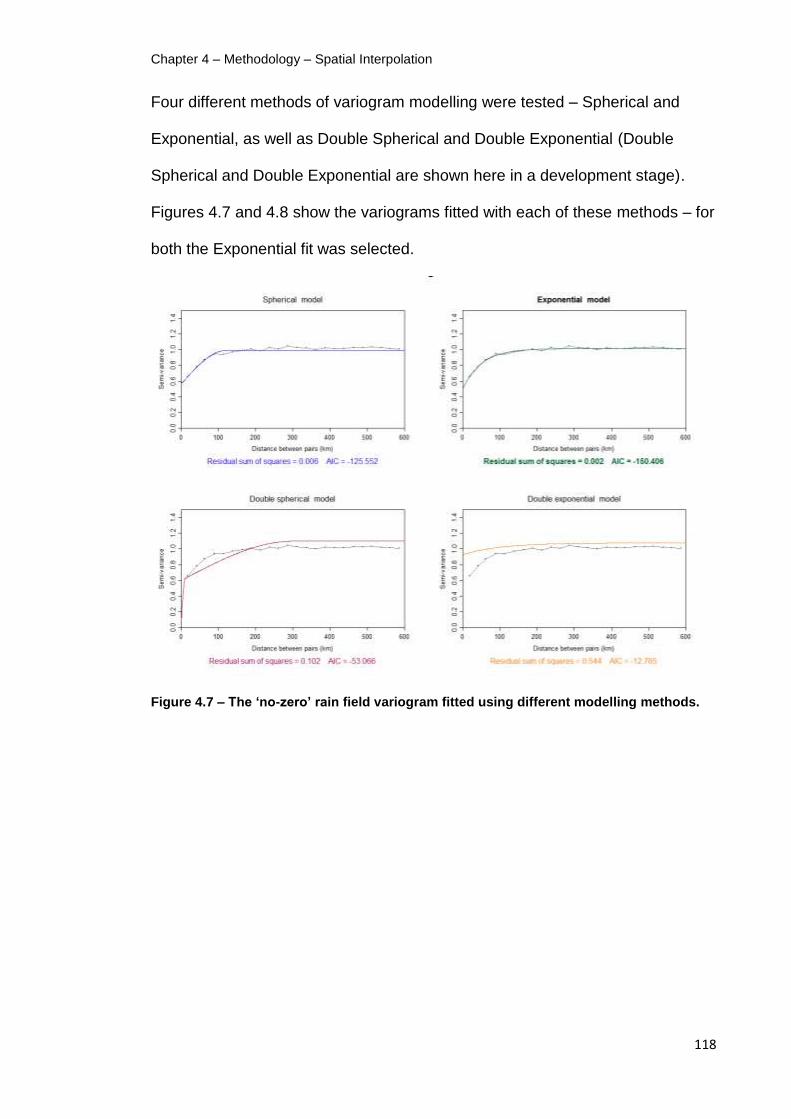
Chapter 4 – Methodology – Spatial Interpolation
118
Four different methods of variogram modelling were tested – Spherical and
Exponential, as well as Double Spherical and Double Exponential (Double
Spherical and Double Exponential are shown here in a development stage).
Figures 4.7 and 4.8 show the variograms fitted with each of these methods – for
both the Exponential fit was selected.
Figure 4.7 – The ‘no-zero’ rain field variogram fitted using different modelling methods.
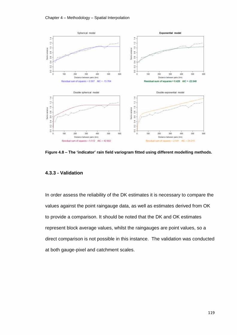
Chapter 4 – Methodology – Spatial Interpolation
119
Figure 4.8 – The ‘indicator’ rain field variogram fitted using different modelling methods.
4.3.3 - Validation
In order assess the reliability of the DK estimates it is necessary to compare the
values against the point raingauge data, as well as estimates derived from OK
to provide a comparison. It should be noted that the DK and OK estimates
represent block average values, whilst the raingauges are point values, so a
direct comparison is not possible in this instance. The validation was conducted
at both gauge-pixel and catchment scales.

Chapter 4 – Methodology – Spatial Interpolation
120
Comparison of Gauge, OK Rain fields and DK Rain fields at Gauge-Pixel Scale
For the comparison, all days where all raingauges recorded zero rainfall were
removed from the record, as their inclusion would only provide trivial results.
Similarly, days where all raingauges recorded rainfall were removed as in these
cases the rain field would not be fractional and the DK method would behave
identically with the OK method, although there were no days recording 100%
rainfall in this dataset. R2 was used as a measure of fit between the data sets.
Figure 4.9 – Charts showing comparison between point raingauge and Kriging estimates
for the block average of pixels containing that raingauge. The chart on the left shows
comparison with OK and the chart on the right shows the comparison with DK. The solid
black line indicates the 1:1 relationship.
Figure 4.9 shows the comparison between the point raingauge data and the
block estimates for the pixels containing gauges, for both OK and DK. The R2
values for both methods indicate that DK more closely resembles the raingauge
rainfall, with a score of 0.52, compared to the score for OK of 0.36. DK was also

Chapter 4 – Methodology – Spatial Interpolation
121
able to predict the fractional field better and was able to match correctly a
pixel’s rainfall status with that of the corresponding raingauge in 86.4% of
cases.
Figure 4.10 – Frequency distribution of raingauge values and block average estimates for
DK and OK. Frequency includes values for zero rainfall that are not shown on the chart,
these were Gauge = 72.7%, DK = 69.4% and OK = 4.1%.
The frequency distributions of rainfalls are shown in Figure 4.10, and it
demonstrates a lack of comparison between the raingauges and block
averaged estimates for DK and OK. DK does compare well in the frequency of
rainfall with raingauges (72.7% zero rainfall for raingauges, 69.4% for DK), yet
the main distribution of rainfall peaks at 12mm, much higher than the raingauge
peak of 2mm. The raingauge data is also more spread, with 4.7% of the rainfall
above 25mm, whilst both OK and DK predicted 1.6% of the rainfall to be above
25mm.

Chapter 4 – Methodology – Spatial Interpolation
122
This is consistent with the findings of Haylock et al. (2008) and Maidment et al.
(in press 2012) who noted that when using block Kriging, grid cell values will
display a different distribution to point values, with the tendency of block values
to converge around the mean rainfall value.
Comparison of Gauge, OK Rain fields and DK Rain fields at Catchment Scale
As previously mentioned, the point raingauge values make for a poor
comparison with the block average Kriged estimates. Catchment average
values for the Bakoye catchment would provide a better comparison and Table
4.1 shows this. For the Kriged estimates, the catchment average was
determined by the mean of the all the pixels within the Bakoye catchment
boundary – for those pixels through which the boundary intersects, the pixel
was split into 100 0.05ºx0.05º pixels and weighted depending on the percentage
of the smaller pixels within the catchment boundary. To compare the catchment
average estimates of rainfall to the raingauge data, an area weighted Gauge
Average estimate was produced using Thiessen Polygons, each adjusted to
account for orographic effects.
Table 4.1 and Figure 4.11 compare the catchment average rainfalls from the
Gauge Average and DK data at various temporal scales. It is seen in Table 4.1
that the DK estimates rainfalls that generally of greater volume than the Gauge
Average, however if the possible error within each of the estimates were to be
considered, the two cannot be distinguished. For example, Nespor and Sevruk
(1998) suggested that wind-induced error alone can cause errors of up to 10%,
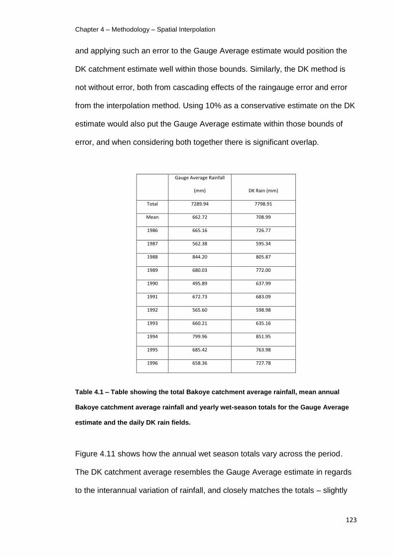
Chapter 4 – Methodology – Spatial Interpolation
123
and applying such an error to the Gauge Average estimate would position the
DK catchment estimate well within those bounds. Similarly, the DK method is
not without error, both from cascading effects of the raingauge error and error
from the interpolation method. Using 10% as a conservative estimate on the DK
estimate would also put the Gauge Average estimate within those bounds of
error, and when considering both together there is significant overlap.
Gauge Average Rainfall
(mm) DK Rain (mm)
Total 7289.94 7798.91
Mean 662.72 708.99
1986 665.16 726.77
1987 562.38 595.34
1988 844.20 805.87
1989 680.03 772.00
1990 495.89 637.99
1991 672.73 683.09
1992 565.60 598.98
1993 660.21 635.16
1994 799.96 851.95
1995 685.42 763.98
1996 658.36 727.78
Table 4.1 – Table showing the total Bakoye catchment average rainfall, mean annual
Bakoye catchment average rainfall and yearly wet-season totals for the Gauge Average
estimate and the daily DK rain fields.
Figure 4.11 shows how the annual wet season totals vary across the period.
The DK catchment average resembles the Gauge Average estimate in regards
to the interannual variation of rainfall, and closely matches the totals – slightly

Chapter 4 – Methodology – Spatial Interpolation
124
estimating more rainfall in most years but indistinguishable with a conservative
estimate of error of 10% applied to each.
Figure 4.11 – Chart showing the annual Bakoye catchment average rainfall totals for the
wet seasons of 1986-1996, for the Gauge Average estimate and the DK daily rain fields.
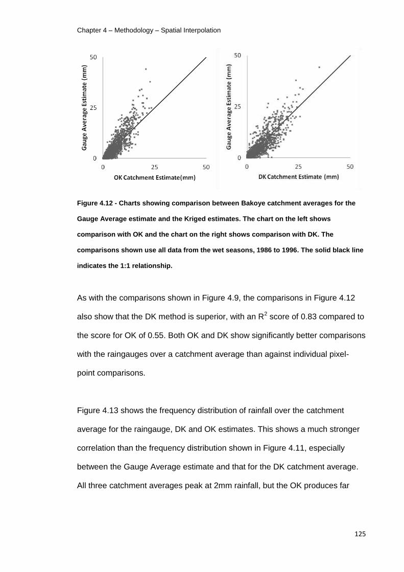
Chapter 4 – Methodology – Spatial Interpolation
125
Figure 4.12 - Charts showing comparison between Bakoye catchment averages for the
Gauge Average estimate and the Kriged estimates. The chart on the left shows
comparison with OK and the chart on the right shows comparison with DK. The
comparisons shown use all data from the wet seasons, 1986 to 1996. The solid black line
indicates the 1:1 relationship.
As with the comparisons shown in Figure 4.9, the comparisons in Figure 4.12
also show that the DK method is superior, with an R2 score of 0.83 compared to
the score for OK of 0.55. Both OK and DK show significantly better comparisons
with the raingauges over a catchment average than against individual pixel-
point comparisons.
Figure 4.13 shows the frequency distribution of rainfall over the catchment
average for the raingauge, DK and OK estimates. This shows a much stronger
correlation than the frequency distribution shown in Figure 4.11, especially
between the Gauge Average estimate and that for the DK catchment average.
All three catchment averages peak at 2mm rainfall, but the OK produces far

Chapter 4 – Methodology – Spatial Interpolation
126
more low level rainfall at the expense of zero rainfall, and rainfall of 11mm or
more.
Figure 4.13 – Frequency distribution of Bakoye catchment average raingauge values and
catchment average estimates of DK and OK. Zero rainfall values are included in the
frequency but not shown on the chart, these were Gauge = 19.5%, DK = 19.3% and OK =
2.9%.
Influence of Spatial Resolution
The sections above have demonstrated the implementation of the DK method
for the Senegal Basin for the generation of daily rain field, which are block
Kriged to a spatial resolution of 0.5° and compared to point rainguage data. It is
unreasonable to assume block averaged DK rainfall estimates will correlate
directly with point data because of the effects of block average, as described by
Maidment et al. (in press 2012). It was possible to produce daily rain field at a
finer spatial resolution for the data available (0.05°), and the difference in the

Chapter 4 – Methodology – Spatial Interpolation
127
rainfall characteristics have been used to observe the effects of spatial
resolution on the block averaging of the DK rain fields.
Figure 4.14 – Frequency distributions of raingauge data and block average values of DK
rainfall at 0.05° and 0.5° pixel resolution. Zero rainfall is included in the frequency but not
shown, these are Gauge = 72.7%, 0.05° = 69.6%, and 0.5° = 69.4%.
Figure 4.14 shows the frequency distribution of rainfall estimates for 0.05°
resolution DK estimate, compared to the point value raingauge values and the
0.5° resolution estimates. It is clear that the influence of the spatial averaging by
block Kriging has a more significant effect on the rainfall estimate than the
difference in spatial resolution, but a slight skewness to lower rainfall values
exists in the distribution when compared to the 0.5° resolution estimate and this
is more in line with the raingauge values.
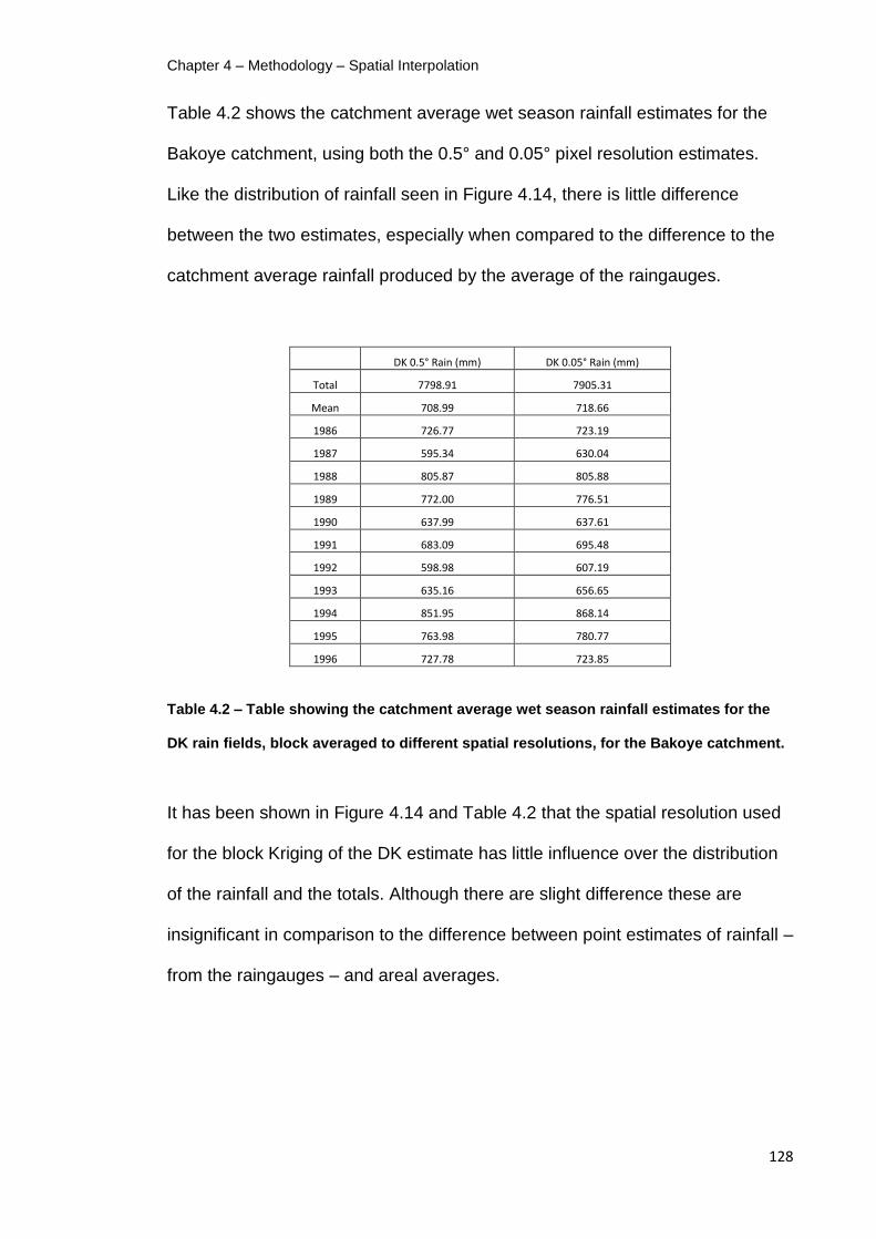
Chapter 4 – Methodology – Spatial Interpolation
128
Table 4.2 shows the catchment average wet season rainfall estimates for the
Bakoye catchment, using both the 0.5° and 0.05° pixel resolution estimates.
Like the distribution of rainfall seen in Figure 4.14, there is little difference
between the two estimates, especially when compared to the difference to the
catchment average rainfall produced by the average of the raingauges.
DK 0.5° Rain (mm) DK 0.05° Rain (mm)
Total 7798.91 7905.31
Mean 708.99 718.66
1986 726.77 723.19
1987 595.34 630.04
1988 805.87 805.88
1989 772.00 776.51
1990 637.99 637.61
1991 683.09 695.48
1992 598.98 607.19
1993 635.16 656.65
1994 851.95 868.14
1995 763.98 780.77
1996 727.78 723.85
Table 4.2 – Table showing the catchment average wet season rainfall estimates for the
DK rain fields, block averaged to different spatial resolutions, for the Bakoye catchment.
It has been shown in Figure 4.14 and Table 4.2 that the spatial resolution used
for the block Kriging of the DK estimate has little influence over the distribution
of the rainfall and the totals. Although there are slight difference these are
insignificant in comparison to the difference between point estimates of rainfall –
from the raingauges – and areal averages.
Chapter 4 – Methodology – Spatial Interpolation
129
4.4 - Summary
The observed raingauge data has been used to obtain the mean daily rainfall
for the Senegal Basin region at an aggregated Meteosat pixel resolution of 0.5º
x 0.5º. A DK method was used so that not just the rainfall amount, but also a
rainy/non-rainy status could be determined for each pixel. The rainfall over the
Senegal Basin region is dominantly fractional, with not a single day in the record
where all functional gauges reported rainfall, and the DK method showed that
86.4% of the pixel estimates for pixels containing a gauge, showed the same
rainfall status of the gauge. The DK estimates compared favourably with the
OK, showing far better correlation with the point raingauge values.
The method presented in this chapter, and results derived from it, are suitable
for use in the calibration of TAMSAT and TAMSIM, but they could be improved.
A co-Kriging technique, such as those described by Goovaerts (2000), could be
employed to incorporate secondary data into the method. This data could be a
DEM of the area to account for the effects of the topography described in
Chapter 3, or for this catchment, it could prove beneficial to account for the
large rainfall gradient across the catchment.
However, the effect of any of these improvements will be limited, just as the
method described in this chapter is, by the paucity of data available for the
study, especially for the Bakoye catchment area which contains just 13
raingauges for over 86,000km2. This lack of raingauges required the method to
be applied to a much wider region in order to produce the necessary variograms
– an area that displays a greater rainfall gradient than that for the catchment

Chapter 4 – Methodology – Spatial Interpolation
130
area alone. Ideally the method would have been employed with a denser set of
raingauges focussed around the Bakoye catchment, as this would have likely
produced a better correlation between the raingauges and the DK estimates.

Chapter 5 – Methodology – Ensemble Representation of Satellite Rainfall Uncertainty
131
5 Methodology – Ensemble
Representation of Satellite Rainfall
Uncertainty
5.1 – Introduction
This chapter is the second of the methodology chapters and details the
methods used to produce a deterministic satellite rainfall estimate (SRFE), and
the methods for characterising the uncertainty within that estimate. The method
used to produce a deterministic SRFE was TAMSAT1, and TAMSIM was used
to characterise the uncertainty. Both methods were introduced by Teo (2006)
and Teo and Grimes (2007).
5.2 – TAMSAT1
Of the available SRFE methods summarised in Chapter 2, the expanded
TAMSAT method of Teo and Grimes (2007) was used to produce daily SRFE
for the Senegal Basin. The method, known as TAMSAT1, was introduced in
Teo (2006) and has some important advantages over the other methods making

Chapter 5 – Methodology – Ensemble Representation of Satellite Rainfall Uncertainty
132
it suitable for this area, namely its ability to be calibrated locally using historic
raingauge networks, its requirement for only a single TIR satellite input and the
long operational history of the method in sub-Saharan Africa. In addition, the
TAMSIM algorithm for characterising the uncertainty has been previously
successfully presented in Teo (2006) and Teo and Grimes (2007) – a significant
advantage of using TAMSAT1.
Previous studies have shown that global SRFE that incorporate PM inputs show
greater skill in estimating rainfall for Africa, over those that only use TIR and/or
raingauges for more complex, mountainous terrain (Dinku et al., 2007 & 2010).
However, the use of PM sensors has limitations for certain types of land surface
which are often mistaken for raining areas (Dinku et al., 2010). In the study by
Dinku et al. (2007) the dekadal TAMSAT estimate was found to outperform all
of the more sophisticated, multi-sensor SRFE, largely attributed to its use of a
regional calibration as opposed to a global calibration. The algorithms that
make use of PM data have yet to be calibrated for the semi-arid regions of
Africa, and such a task is complicated as it would require a large volume of
ground data that is unlikely to be available (Morland et al., 2001).
As TIR based SRFE generally rely upon an indirect relationship between cloud
top temperature and actual rainfall, the rainfall estimations contain significant
uncertainties, principally in three aspects:
1. Temporal - When it is raining
2. Spatial - Where it is raining

Chapter 5 – Methodology – Ensemble Representation of Satellite Rainfall Uncertainty
133
3. Rate - How much it is raining
The TAMSAT method, and TAMSAT1, is subject to these uncertainties and
therefore there is a requirement for an accurate and appropriate method to
characterise this uncertainty, in such a way that can be translated into
downstream applications.
The TAMSAT1 method has been selected for the generation of a deterministic
SRFE for the Senegal Basin area, at a daily time-step. Teo and Grimes (2007)
introduced the TAMSAT1 method, an extension of the TAMSAT method, to
produce daily rainfall estimates. This section provides a summary of the
method, a comprehensive methodology can be found in Teo (2006). The
method implemented here is a modification to that of Teo (2006), in that it does
not include a representation of the DK error which was sacrificed to allow for a
more accurate method of modelling the gamma distribution of no-zero DK
rainfall at gauge-pixels plotted at bins.
The TAMSAT method, as described in the previous section, uses a locally
calibrated relationship between cloud top temperature and the historic
raingauge record. A full description of the method can be found in Milford and
Dugdale (1990). TAMSAT uses a Cold Cloud Duration (CCD) technique, where
Meteosat TIR data is used to obtain cloud top temperatures at 15 minute time-
steps with cloudy pixels below a specified temperature threshold assumed to be
rainy – cold clouds are associated with high topped cumulonimbus clouds,
synonymous with convective rainfall. The total period in a day that a pixel is

Chapter 5 – Methodology – Ensemble Representation of Satellite Rainfall Uncertainty
134
below the threshold is its CCD, or . For TAMSAT the CCD represents the
total period below the threshold for a given dekad and is used to calculate a
dekadal estimate of rainfall, .
Equation 5.1
Equation 5.1 shows the simple linear relationship used to generate the dekadal
estimate of rainfall, , using the TAMSAT method. The values for the
parameters and are calibrated by plotting CCD values against DK rainfall
values for pixel’s containing at least one raingauge (gauge-pixels).
The linear relationship used in Equation 5.1 has been found to be successful at
dekad scale (Dinku et al., 2007), but is too simplistic to represent the more
spatially and temporally varied nature of daily rainfall. Of particular importance
is the representation of the fractional nature of the rainfall field which is greater
at smaller time-steps. In order to address these issues Teo (2006) developed
the TAMSAT1 method and found that it outperformed the original TAMSAT
method for estimation of daily rainfall fields for the Gambia region. Equation 5.2
shows the calculation of daily rainfall, at pixel location in its simplest form,
and is expanded below.
Equation 5.2

Chapter 5 – Methodology – Ensemble Representation of Satellite Rainfall Uncertainty
135
Equation 5.2 shows the principal of TAMSAT1, where the rainfall is the product
of the probability of rainfall at , , and the mean rainfall at with the zero
values removed, . The calculation of is shown in Equation 5.3 and the
calculation of is shown in Equation 5.4.
Equation 5.3
The parameters and are found by plotting the probability of rainfall from the
DK gauge-pixels against , and fitting the relationship using logistic
regression. The probability of rainfall at , , is excluded from the fit and
the actual probability is used instead.
Equation 5.4
In Equation 5.4, is the mean rainfall at , derived from gamma fits of no-zero
DK rainfall at gauge-pixels plotted at bins, using a maximum likelihood
method (n.b. – the original method in Teo (2006) used a method of moments
fit). The shape and rate functions of each gamma distribution are modelled to
so that a linear relationship between mean rainfall and is produced,
when is equal to the product of the shape and rate functions. This linear
relationship is expressed in Equation 5.4.
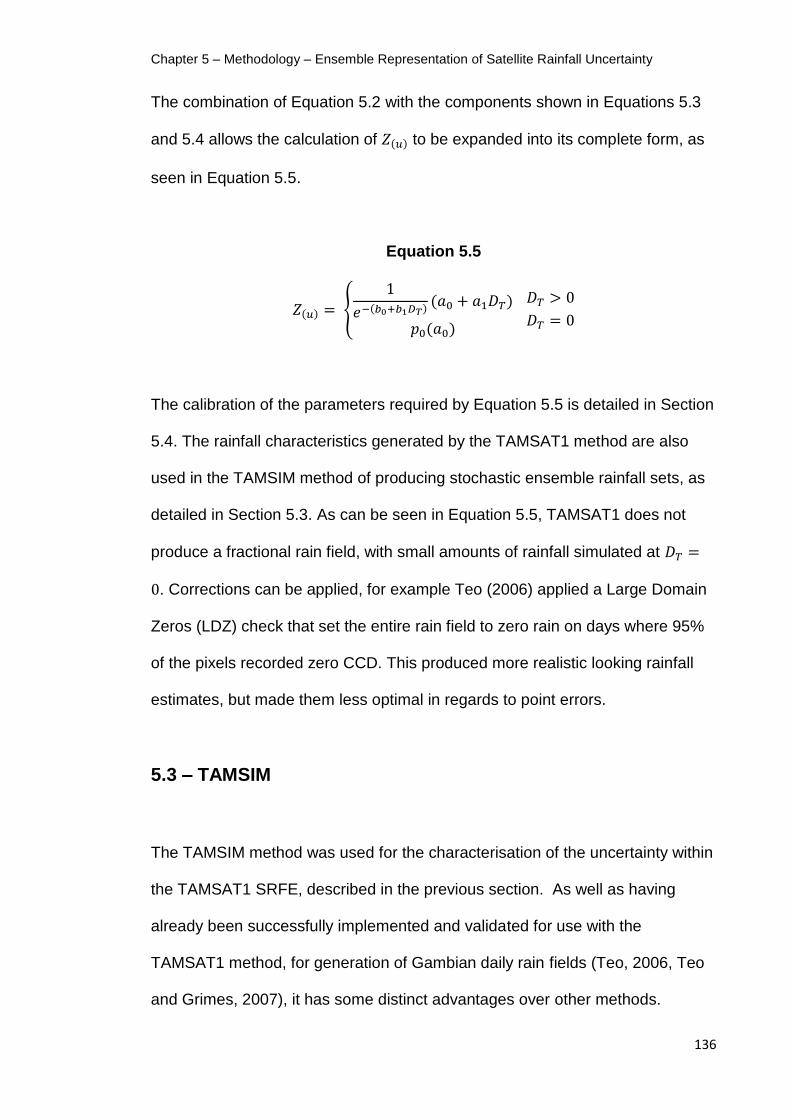
Chapter 5 – Methodology – Ensemble Representation of Satellite Rainfall Uncertainty
136
The combination of Equation 5.2 with the components shown in Equations 5.3
and 5.4 allows the calculation of to be expanded into its complete form, as
seen in Equation 5.5.
Equation 5.5
The calibration of the parameters required by Equation 5.5 is detailed in Section
5.4. The rainfall characteristics generated by the TAMSAT1 method are also
used in the TAMSIM method of producing stochastic ensemble rainfall sets, as
detailed in Section 5.3. As can be seen in Equation 5.5, TAMSAT1 does not
produce a fractional rain field, with small amounts of rainfall simulated at
. Corrections can be applied, for example Teo (2006) applied a Large Domain
Zeros (LDZ) check that set the entire rain field to zero rain on days where 95%
of the pixels recorded zero CCD. This produced more realistic looking rainfall
estimates, but made them less optimal in regards to point errors.
5.3 – TAMSIM
The TAMSIM method was used for the characterisation of the uncertainty within
the TAMSAT1 SRFE, described in the previous section. As well as having
already been successfully implemented and validated for use with the
TAMSAT1 method, for generation of Gambian daily rain fields (Teo, 2006, Teo
and Grimes, 2007), it has some distinct advantages over other methods.

Chapter 5 – Methodology – Ensemble Representation of Satellite Rainfall Uncertainty
137
Importantly, TAMSIM retains the geostatistical properties of the raingauge
derived rainfall field and allows for the generation of fractional rainfall fields. As
the Senegal Basin shows a large rainfall gradient (see Chapter 3), it is important
that the ensemble rain fields are able to distinguish between the areas where it
is raining and the areas where it is not.
With the uncertainty within the SRFE characterised, it needs to be translated to
a downstream application to measure the extent of propagation. In Teo (2006)
and Teo and Grimes (2007) this was a crop yield model, and for this thesis this
will be a hydrological model.
The remainder of this section presents a methodology for the TAMSIM
algorithm, as introduced by Teo (2006) and Teo and Grime (2007), where a
comprehensive methodology can be seen.
In its simplest form the equation governing TAMSIM is the same as Equation
4.1, the Equation used for DK from Barancourt et al. (1992). In this case, the
two RFs, and , are generated using sequential sequencing techniques
outlined below. The TAMSIM algorithm is thus divided into two separate
algorithms that calculate the two necessary RFs:
1. Sequential Indicator Simulation (sIs) – produces a binary rain/no-rain
‘indicator’ field demarcating the areas that are rainy and those that are
not.

Chapter 5 – Methodology – Ensemble Representation of Satellite Rainfall Uncertainty
138
2. Sequential Gaussian Simulation (sGs) – produces a rainfall field by
simulating rainfall amounts for the pixels identified as rainy during sIs.
This section will look at the sIs and sGs stages separately before demonstrating
how TAMSIM combines them.
Sequential Indicator Simulation (sIs)
The first stage of the TAMSIM algorithm is the sIs that produces a binary RF of
rain/no-rain areas. Before running it requires a calibration of the probability of
rainfall at each specified CCD bin and this is derived using Equation 5.3, in the
same way as for TAMSAT1. The method also uses a simple Kriging (SK)
method and this requires a variogram of the indicator residuals to be produced.
More details of the TAMSIM calibrations can be found in Section 5.4.
Figure 5.1 shows a schematic taken from Teo and Grimes (2007) detailing the
steps taken by sIs to produce the indicator RF, for a theoretical nine cell grid.

Chapter 5 – Methodology – Ensemble Representation of Satellite Rainfall Uncertainty
139
Figure 5.1 – Schematic from Teo and Grimes (2007) showing the steps required for the
operation of the sIs algorithm on a theoretical nine cells system. The steps are (i) input
initial CCD values for each pixel. (ii) CCD values are substituted with the probability of
rain at that CCD using Equation 5.3. (iii) Independent seed pixels are selected and given a
rain/no-rain status via Bernoulli trail. (iv) Residuals are calculated for each of the seed
pixels by subtracting the probability of rain for that pixel from the binary rainfall status it
was assigned. A random path is determined for the remaining pixels A-G. The residuals
are used to produce a residual value for pixel A using simple Kriging (SK). (v) The
residual value for pixel A is added to the probability of rain for the pixel for its total
probability of rainfall. (vi) Pixel A is assigned a rain/no-rain status, based on the
probability of rainfall at that pixel’s CCD value, and is added to the set of seed pixels. (vii)
Steps iii-vi are repeated until each pixel is assigned a rainfall status.
Sequential Gaussian Simulation (sGs)
After producing the indicator RF via sIs, TAMSIM then uses this field to start the
sGs stage to estimate rainfall for each pixel designated as raining. This step
requires a distribution of rainfall to be modelled for each specified CCD bin, and

Chapter 5 – Methodology – Ensemble Representation of Satellite Rainfall Uncertainty
140
this was done by modelling a gamma distribution by fitting to CCD-binned no-
zero DK rain data, in the same way as described for TAMSAT1. The shape and
rate functions are then modelled in a way to produce a linear fit of mean rainfall.
In addition, sGs requires a variogram of no-zero rainfall residuals to be
produced. Further details of the calibration can be found in Section 5.4.
Figure 5.2 shows a step-by-step schematic of the sGs process, taken from Teo
and Grimes (2007).
Figure 5.2 – Schematic from Teo and Grimes (2007) showing the steps taken by the sGs
algorithm, for the same theoretical nine cells system shown in Figure 5.1. (i) CCD values
for pixels designated as raining by sIs are inputted. (ii) Independent seed pixels are
selected and allocated Gaussian residual values. A random path is assigned for the
remaining pixels A-C. (iii) A Gaussian residual value is calculated for pixel A by SK of the
seed pixels. (iv) A final residual value is assigned to Pixel A by sampling within the SK
bounds, and is added to the set of seed pixels. (v) Steps iii and iv are repeated until all
pixels are assigned a Gaussian residual value. (vi) The Gaussian residuals are back-
transformed and added to the original estimate for that pixel’s CCD value, providing an
estimate of rainfall for that pixel.

Chapter 5 – Methodology – Ensemble Representation of Satellite Rainfall Uncertainty
141
Combining the Field – Producing Ensembles
By combination of a single sIs field and a single sGs field the TAMSIM algorithm
will produce a single ensemble representation of a probable rainfall field. The
algorithm produces a set of equiprobable ensemble members by combining the
two fields, saving computational time by running the sGs algorithm multiple
times for each sIs realisation.
5.4 – Implementation of TAMSAT1 and TAMSIM
5.4.1 – Introduction
This section looks at the implementation of the TAMSAT1 algorithm, its
calibration, production of a deterministic estimate of the rainfall field and the
validation of that field. The TAMSIM algorithm shares much of the same
calibration procedure as TAMSAT1, and the necessary extensions for TAMSIM
are also detailed here.
Both the TAMSAT1 and TAMSIM rainfall fields were produced using a modified
version of the Genrain (SIMU) algorithm in the Matlab environment, written by
Teo (2006) and provided by Dr David Grimes, Department of Meteorology,
University of Reading.

Chapter 5 – Methodology – Ensemble Representation of Satellite Rainfall Uncertainty
142
5.4.2 – Calibration
The TAMSAT1 and TAMSIM algorithms were detailed in Sections 5.2 and 5.3.
The calibration of TAMSAT1 can be split into three stages:
Determination of the optimal temperature threshold
Determining the probability of rainfall at CCD
Determination of positive rainfall rate at CCD
Determining the optimal temperature threshold
A suitable temperature threshold (T) needs to be identified for determining the
Cold Cloud Duration (CCD) for each pixel of the satellite image – the threshold
being the temperature below which a cloud can be said to be rainy. The
TAMSAT CCD data is provided at 0.05°x0.05° pixel resolution, but as it was not
possible to complete the test at this resolution it was necessary to aggregate
the data to 0.5°x0.5° pixels to match the pixels representing the DK rain fields.
This was taken as the mean CCD of every pixel within corresponding DK pixels.
The most suitable temperature threshold was selected by directly comparing the
CCD data with the indicator field from the DK data, for gauge-pixels only –
those pixels which contain at least one raingauge. Table 5.1 shows a
contingency table used as part of the calibration, where Z is the rainfall of a DK
gauge-pixel and is the CCD at the same gauge-pixel at a particular
temperature threshold. The calibration was conducted for daily rainfall and

Chapter 5 – Methodology – Ensemble Representation of Satellite Rainfall Uncertainty
143
CCD, using only the wet season data. Ideally an individual calibration would be
performed for each month, however due to the paucity of data available only a
single calibration was conducted for the whole wet season. Similarly, because
of the large area used for the study, zonal calibrations would have been useful
but not possible in this circumstance.
DT=0 DT>0
Z=0 n11 n12
Z>0 n21 n22
Table 5.1 – Example contingency table for the selection of a temperature threshold for
TAMSAT CCD (T) (after Teo, 2006).
The selected temperature threshold is the one that best satisfies the selection
criteria outlined by Milford and Dugdale (1990) and Grimes et al. (1999), which
can be summarised as:
Criteria 1 =
>> 1
Criteria 2 =
≈ 1
The TAMSAT CCD data is provided at temperature thresholds of -20°C, -30°C,
-40°C, -50°C and -60°C.
Table 5.2 shows the calibration data for the Senegal Basin area for the study
period, at each available temperature threshold. A ‘hit’ is when a gauge-pixel
shows either both zero rainfall and zero CCD, or positive rainfall and positive

Chapter 5 – Methodology – Ensemble Representation of Satellite Rainfall Uncertainty
144
CCD. All other cases are ‘misses’. The best performing temperature threshold
is -60°C, where 65.35% of the gauge-pixels showed a hit. This is similar to that
determined by Teo (2006) for the Gambia region, where the -60°C was selected
for each month of the wet season, except for August where -50°C was used.
CCD Threshold
(°C) DT=0 DT >0 Total Criteria 1 Criteria 2 % correct
-20
Z=0 34573 34261
103696 1.29 0.25 53.45
Z>0 8611 20851
DT =0 DT >0 Total
-30
Z=0 41305 27951
103696 1.53 0.40 57.58
Z>0 11080 18401
DT =0 DT >0 Total
-40
Z=0 46921 22801
103696 1.73 0.59 60.64
Z>0 13510 15964
DT =0 DT >0 Total
-50
Z=0 52783 17588
103696 1.94 0.93 63.52
Z>0 16441 13088
DT =0 DT >0 Total
-60
Z=0 58625 11600
103696 2.14 1.73 65.35
Z>0 20098 9138
Table 5.2 – TAMSAT temperature threshold calibration table, where z represents DK
rainfall at gauge-pixels and DT represents the CCD at gauge-pixels at specified threshold.
Determination of Probability of Rain at CCD
The calibration of probability of rain at CCD was conducted by comparing DK
and CCD gauge-pixel data. The DK was converted to a binary rain/no-rain field
and the CCD data was binned to nearest CCD hour ( ). The probability of rain

Chapter 5 – Methodology – Ensemble Representation of Satellite Rainfall Uncertainty
145
at each CCD hourly bin was calculated from the DK gauge-pixel data, and
modelled by fitting using logistic regression. As shown in the methodology in
Section 5.3, it is necessary to estimate the empirical constants of b0 and b1,
when –
where is the sample probability of rainfall at .
The empirical constants b0 and b1 are then used to model using the equation
–
As there were too few values corresponding to DT>8, these were excluded from
the fit. As the probability of rain at DT=0 is much less than at DT>0, this too was
excluded from the fit, and the actually probability of rain at DT=0 was used
instead. The fitted relationship between the probability of rain and CCD is
shown in Figure 5.3.

Chapter 5 – Methodology – Ensemble Representation of Satellite Rainfall Uncertainty
146
Figure 5.3 – Chart showing the modelled relationship between probability of rain and
CCD at hourly bins (DT).
Determination of Positive Rainfall Rate at CCD
To determine the rainfall rate at CCD for use in the TAMSIM algorithm the DK
gauge-pixel data, with zero rainfall values removed, was compared against the
CCD gauge-pixel sorted into hourly bins. A gamma distribution was fitted to the
rainfall at each of these hourly bins.
Teo (2006) used a method of moments technique for fitting the gamma
distributions, but for this thesis a maximum likelihood technique was used
instead as it provides a better fit for the distributions. The simple representation
of DK error used by Teo (2006) was not directly transferable to the maximum
likelihood method used in this thesis and has not been included.
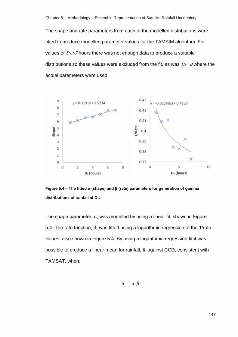
Chapter 5 – Methodology – Ensemble Representation of Satellite Rainfall Uncertainty
147
The shape and rate parameters from each of the modelled distributions were
fitted to produce modelled parameter values for the TAMSIM algorithm. For
values of DT>7 hours there was not enough data to produce a suitable
distributions so these values were excluded from the fit, as was DT=0 where the
actual parameters were used.
Figure 5.4 – The fitted α (shape) and β (rate) parameters for generation of gamma
distributions of rainfall at DT.
The shape parameter, α, was modelled by using a linear fit, shown in Figure
5.4. The rate function, β, was fitted using a logarithmic regression of the 1/rate
values, also shown in Figure 5.4. By using a logarithmic regression fit it was
possible to produce a linear mean for rainfall, against CCD, consistent with
TAMSAT, when:

Chapter 5 – Methodology – Ensemble Representation of Satellite Rainfall Uncertainty
148
The relationship between modelled mean rainfall against CCD is shown in
Figure 5.5.
Figure 5.5 – Fitted mean rainfall at DT. Mean rainfall at DT=0 is not included in the fit and
the mean is derived from the actual mean.
5.4.3 – Validation of the TAMSAT1 SRFE
A deterministic SRFE has been produced for the Senegal Basin, for the wet
seasons of the study period (1986-1996), using the TAMSAT1 method. The
daily rain fields produced were clipped to the Bakoye catchment to produce a
catchment average TAMSAT1 estimate for use in the Pitman model. The
TAMSAT1 method was validated for the Bakoye catchment by comparing the
characteristics of the catchment average TAMSAT1 estimate to the catchment
average DK estimates. Table 5.3 shows the totals of these catchment average
rainfalls at various temporal scales.

Chapter 5 – Methodology – Ensemble Representation of Satellite Rainfall Uncertainty
149
DK Rain (mm) TAMSAT1 Rain (mm)
Total 7798.91 7227.58
Mean 708.99 657.05
1986 726.77 628.28
1987 595.34 641.72
1988 805.87 726.89
1989 772.00 636.52
1990 637.99 685.87
1991 683.09 649.99
1992 598.98 657.55
1993 635.16 617.84
1994 851.95 697.28
1995 763.98 676.27
1996 727.78 609.36
Figure 5.3 – Table showing the total catchment average rainfall, mean annual Bakoye
catchment average rainfall and yearly wet-season totals for DK and TAMSAT1 daily rain
fields.
Figure 5.6 – Bar chart showing the annual Bakoye catchment average rainfall totals for
the wet seasons of 1986-1996, for raingauge data, the DK and TAMSAT1 daily rain fields.

Chapter 5 – Methodology – Ensemble Representation of Satellite Rainfall Uncertainty
150
Table 5.3 and Figure 5.6 compare the catchment average rainfalls for the DK
and TAMSAT1 rainfall estimates for the entire 11 year period (wet seasons
only), and for each individual wet season. The TAMSAT1 catchment averages
estimate a lower level of rainfall than the DK catchment averages, although
even using a conservative estimate of error (due to raingauge measurement
and interpolation errors) of 10% the three estimates of rainfall show significant
overlap and could be said to be indistinguishable. However, the TAMSAT1
catchment averages also fail to reproduce the interannual variation evident in
the DK catchment averages – this is caused by the use of a climatic calibration,
which will cause smoothing of interannual variability and introduces a
systematic bias for years of anomalous rainfall.
Figures 5.7 and 5.8 compare the distributions of catchment average rainfalls for
the TAMSAT1 estimate and the DK estimate. TAMSAT1 does not produce a
fractional rainfall field and as such does not model any zero rainfall in the
record. This results in greater frequency of low level rainfall, especially 1.5-
2.5mm.
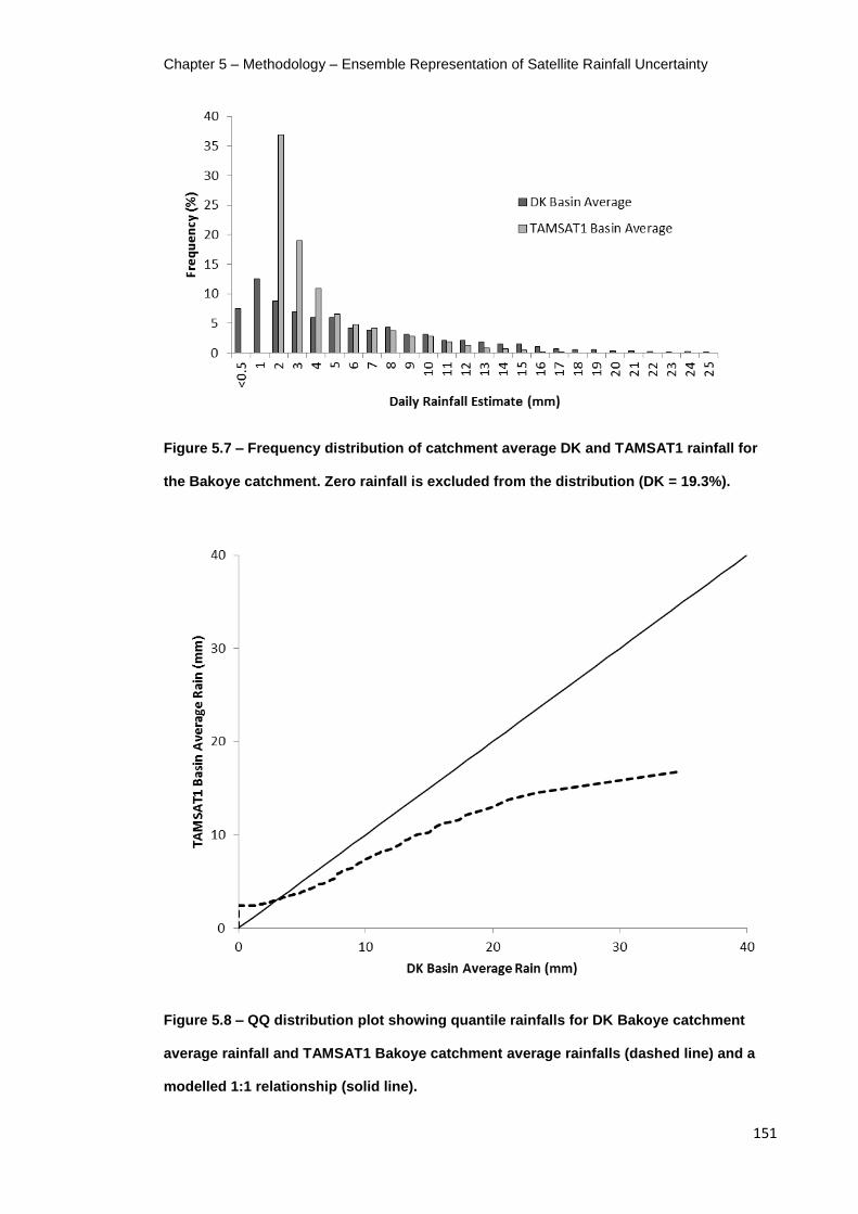
Chapter 5 – Methodology – Ensemble Representation of Satellite Rainfall Uncertainty
151
Figure 5.7 – Frequency distribution of catchment average DK and TAMSAT1 rainfall for
the Bakoye catchment. Zero rainfall is excluded from the distribution (DK = 19.3%).
Figure 5.8 – QQ distribution plot showing quantile rainfalls for DK Bakoye catchment
average rainfall and TAMSAT1 Bakoye catchment average rainfalls (dashed line) and a
modelled 1:1 relationship (solid line).

Chapter 5 – Methodology – Ensemble Representation of Satellite Rainfall Uncertainty
152
5.4.4 – Implementation of TAMSIM
In addition to the calibrated relationships above, the TAMSIM algorithm requires
three further steps for implementation. These are –
Generation of indicator residuals and variogram
Generation of no-zero rainfall residuals and variogram
Parameters required for generation of ensembles
Generation of Indicator Residuals and Variogram
The calculation of residual values at each gauge-pixel is required for the
generation of the residual variogram, the parameters of which are a key
requirement for the TAMSIM algorithm. The residual for each gauge-pixel is
binary rain status of the pixel (0 = no rain, 1 = rainy), minus the probability of
rain at the corresponding CCD hourly bin. The residual values at each gauge-
pixel are then used to generate a variogram using KrigeRain in the same way
as demonstrated in Chapter 4. Figure 5.9 shows the residual indicator
variogram and its parameters.

Chapter 5 – Methodology – Ensemble Representation of Satellite Rainfall Uncertainty
153
Figure 5.9 – Residual ‘indicator’ variogram and parameters for use in the TAMSIM
algortithm.
Generation of No-Zero Rainfall Residuals and Variogram
To generate a no-zero residual variogram it is necessary to first calculate
residuals values for no-zero rainfall at gauge-pixels. For each gauge-pixel no-
zero rainfall value, the probability of that rainfall occurring on the gamma
distribution of the corresponding CCD hourly bin is found, and the residual is
then calculated by applying that probability to an inverse normal distribution,
with a mean of zero and standard deviation of 1. As with the indicator residuals
the residuals are used to generate a residual variogram using KrigeRain. The
residual no-zero variogram is shown in Figure 5.10.

Chapter 5 – Methodology – Ensemble Representation of Satellite Rainfall Uncertainty
154
Figure 5.10 – Residual ‘no-zero’ variogram and parameters for use in the TAMSIM
algorithm.
Parameters Required for Producing Ensembles.
TAMSIM produces individual ensemble members by combining an indicator
field with a no-zero rain field. A description of the methodology has been given
in Section 5.3. Teo (2006) showed that at least 200 ensemble members were
required for the mean and variance to converge in experimentations, so 200
ensembles were produced. It is not necessary to produce unique indicator
fields and no-zero fields for each individual ensemble member, as fields can be
combined to produce unique realisations. For this thesis 50 indicator fields and
4 no-zero rain fields were produced, for a total of 200 unique yet equiprobable
ensemble rain fields. A validation and analysis of TAMSIM can be found in
Chapter 7.

Chapter 5 – Methodology – Ensemble Representation of Satellite Rainfall Uncertainty
155
5.5 - Summary
This chapter has shown the methodologies for TAMSAT1, used to produce a
deterministic SRFE for the Senegal Basin. It has shown its calibration and
implementation for the region, and a catchment average estimate has been
calculated for the Bakoye catchment which is used as an input to drive the
Pitman lumped CRR model (as demonstrated in Chapter 6). The Bakoye
catchment average TAMSAT1 estimate has been validated against the DK
catchment average for the Bakoye catchment, finding that it compares
favourably in regards to the volumes of rainfall, but fails to fully reflect the
interannual variability of rainfall – likely a result of the use of a climatic
calibration.
To characterise the uncertainty within the TAMSAT1 estimates, the TAMSIM
algorithm was used, and Section 5.3 provided the methodology. Section 5.4
showed how TAMSIM was calibrated and used to produce 200 unique, yet
equiprobable realisations of the daily Senegal Basin rain field.
Chapter 6 is the final of the three methodology Chapters and demonstrates the
methodology for the Pitman lumped CRR model, and its calibration using the
Shuffled Complex Evolution (SCE-UA) method. The characteristics of the
TAMSIM ensemble SRFE are assessed in Chapter 7, and the propagation of
the uncertainty they reflect is detailed in Chapters 8 and 9.

Chapter 6 – Methodology – Hydrological Modelling
156
6 Methodology – Hydrological
Modelling
6.1 – Introduction
This chapter is the final of three methodology chapters and details the methods
used for the hydrological modelling of the Bakoye catchment. The model used
was the Pitman model, a lumped conceptual rainfall-runoff (CRR) model, with
11 adjustable parameter values. The calibration was carried out using an
automatic optimisation algorithm, the Shuffled Complex Evolution model
implemented at the University of Arizona (SCE-UA).
6.2 – The Pitman Model
The Pitman model is a lumped CRR model introduced by Pitman (1973), and
has been used widely across Africa with success in applications involving water
resources assessments (Middleton et al., 1981, Hughes, 1995). The
unmodified, monthly model has 2-buckets and 12 parameters.

Chapter 6 – Methodology – Hydrological Modelling
157
Hughes et al. (2006) applied a modified Pitman model to the Okavango Basin in
south-west Africa, modelling 24 sub-catchments using raingauge and TRMM
SRFE as rainfall inputs to drive the models at a monthly timestep. Hughes et al.
(2006) found that the calibrated Pitman models could represent catchment
response to SRFE satisfactorily for periods outside the calibration period,
claiming that other CRR models were unlikely to perform significantly better
than the Pitman model, but no others were tested.
The Pitman model, modified to model daily rainfall instead of monthly, was used
to model the catchment response of the upstream sub-catchments of the
Senegal Basin to TAMSAT SRFE in Hardy et al. (1989) and Grimes and Diop
(2003). Both studies found the Pitman model performed well with both a
raingauge rainfall estimate and the TAMSAT estimate. Grimes and Diop (2003)
applied the Pitman model to the Bakoye catchment itself.
The modified daily Pitman model used by Grimes and Diop (2003) has been
used in this thesis. With previous studies having successfully applied the
Pitman model to the region and the actual study site, it has been shown to
perform well in these conditions. Additionally the previous studies can provide a
suitable comparison to the model outputs produced.
Methodology
The Pitman model is a lumped CRR model, first developed by Pitman (1973),
modified to run at a daily timestep. This model was used in Grimes and Diop

Chapter 6 – Methodology – Hydrological Modelling
158
(2003) and was provided through personal correspondence with David Grimes
(2009). The model is summarised in Figure 6.1.
Figure 6.1 – The Pitman Model (from Grimes and Diop, 2003). (Key terms – P
(Precipitation Input), I (Interception Storage, Imax = maximum storage), W (Soil Moisture,
Wmax = maximum storage), G (Groundwater), Ei (Evaporation from Interception Storage),
Es (Evaporation from Soil Moisture), Ep (Potential Evaporation), Z (Infiltration Rate Zmin
and Zmax = minimum and maximum rates), Qq (Quick, or surface flow rate), Qq1 (Quick
flow of rainfall rate exceeding Zmax), Qq2 (Quick flow from saturated soil), Qb (Baseflow
rate), Q (Total discharge flow rate, sum of appropriately lagged Qq and Qb). i and h are
empirical values.
The Pitman model shown in Figure 6.1 requires only daily rainfall and potential
evaporation as an input and its operation at a daily timestep can be summarised
as –
Rainfall (P) added to the surface store (I) and allowed to evaporate (Ei)

Chapter 6 – Methodology – Hydrological Modelling
159
The remaining water infiltrated to the soil moisture (W), unless the
maximum threshold (Imax) is exceeded, in which case the excess runs off
as surface flow (Qq1)
Water in W either percolates (Qp) to the groundwater store (G), or
evaporates (Es). If the maximum threshold of the soil moisture store
(Wmax) is exceeded then the excess rainfall runs off as surface flow (Qq2).
Water stored in G flows out at a specified rate (Qb)
Lagged combined surface flow (Qq) and baseflow (Qb) are summed for
the daily discharge (Q)
For the calibration of the Pitman model there are eleven variable parameters, in
addition to the daily inputs and a value corresponding to the catchment area.
These parameters, and an initial set of parameter values, provided by David
Grimes (personal correspondence, 2009), can be seen in Table 6.1.
Although the initial parameter set provided in Table 6.1 provides a suitable
starting point for calibration, it should be noted that it does not allow for the full
complexity of the model to be utilised. The value provided for h, being 0, does
not allow for any percolation from the soil moisture store to the groundwater
stores, restricting the model to operating as a 1-bucket model. Although this
may suit the catchment, the calibration will allow for the Pitman model to
operate as a 2-bucket model and use its full complexity.

Chapter 6 – Methodology – Hydrological Modelling
160
Parameter Description Value Units
Zmin Minimum infiltration rate 0 mm.day-1
Zmax Maximum infiltration rate 23 mm.day-1
Wmax Storage threshold of Soil Moisture 460 mm
Wmin Storage threshold below which no percolation occurs 0 mm
Imax Storage threshold of Interception Storage 1 mm
h Empirical constant used to calculate percolation rate 0 mm.day-1
i Empirical constant used to calculate percolation rate 2
GL Recession time constant for baseflow (G0 = 1/GL) 3 days
TL Contant used for calculation of the surface flow 11 days
Qq Lag Lag for surface (quick) flow 1 days
Qb Lag Lag for baseflow 1 days
Table 6.1 – Table showing the variable parameters in the Pitman model to be calibrated,
and an initial set of parameter values provided by David Grimes (personal
correspondence, 2009).
6.3 - The Shuffled Complex Evolution method implemented at
the University of Arizona (SCE-UA)
A popular method of automatic optimal calibration is the Shuffled Complex
Evolution (SCE) method implemented at the University of Arizona (Duan et al.,
1993). Duan et al. (1993) details the SCE algorithm, based around four
components –
1. A mix of deterministic and probabilistic approaches
2. Clustering
3. A systematic evolution of a complex of points within the parameter
space, towards improvement

Chapter 6 – Methodology – Hydrological Modelling
161
4. Competitive evolution
SCE is a global optimisation method in that it is able to examine the entire
parameter space, identify the areas of local minima and narrow down the
search before refining the final optimal parameter set (Duan et al., 1993), as
opposed to a local minima optimisation method that is dependent on a suitable
initial set of parameters (Wang et al., 2010). The method has been shown to be
successful at estimating reliable optimal parameter sets for complex CRR
models (Duan et al., 1994), and outperforming other global optimisation
techniques available at the time (Duan et al., 1993).
The method is widely used and still found to perform well. Wang et al. (2010)
found that of three global optimisation methods, SCE was the most robust
although all the methods produced similar outcomes. There have been efforts to
improve the technique, such as the Shuffled Complex Evolution Metropolis
(SCEM) (Vrugt et al., 2003) which adapted the Monte Carlo Markov Chain
(MCMC) method within the model, and the Shuffled Complex with Principal
Component Analysis (SP-UCI) (Chu et al., 2010), however, the core principals
of the original algorithm have been retained.
Another adaption of the original SCE-UA algorithm was demonstrated by Yapo
et al. (1998) with the Multi-Objective Complex Evolution (MOCOM-UA) global
optimisation method, which fits the parameters by calibrating to more than one
objective function. A similar method was applied to the MIKE SHE distributed
model in Madsen (2003). Although this method could potential produce a

Chapter 6 – Methodology – Hydrological Modelling
162
hydrograph that better reflects the recorded discharge, it is likely to prove
computationally expensive, and not provide a single measure of goodness-of-fit
for use in comparisons which the SCE-UA can provide.
Methodology
As previously stated, the SCE-UA method was implemented at the University of
Arizona and introduced in Duan et al. (1993). It is a global optimisation method
that has been widely used for hydrological model calibration and shown to be
robust (see above). This section provides a summary of the algorithm, a full
methodology can be found in Duan et al. (1993).

Chapter 6 – Methodology – Hydrological Modelling
163
Figure 6.2 – Flow chart showing the main steps required for shuffled complex evolution
(from Duan et al., 1993) – The CCE algorithm can be seen in Figure 6.3.

Chapter 6 – Methodology – Hydrological Modelling
164
Figure 6.3 – Flow chart of the Competitive Complex Evolution (CCE) strategy, part of the
SCE algorithm shown in Figure 6.2 (from Duan et al., 1993).

Chapter 6 – Methodology – Hydrological Modelling
165
The flow charts shown in Figures 6.2 and 6.3 describe the full method of the
SCE algorithm and the incorporated Competitive Complex Evolution (CCE)
strategy. The SCE process can be summarised as:
1. Set up the algorithm – decide number of complexes to use and number
of points in each complex
2. The algorithm generates a sample within the reasonable space
3. The points sampled are ranked depending on model performance and
stored in an array
4. The space is partitioned into complexes of equal points
5. Each complex is evolved according to the CCE strategy detailed below,
and shown in Figure 6.3
6. The complexes are shuffled according to model performance
7. Check whether the model performance has reached the convergence
criteria. If not, the algorithm returns to step 3.
The CCE strategy can be summarised as:
1. Initialise the algorithm – decide on number of iterations to run
2. Weights are assigned to each point via a triangular probability distribution
3. Randomly select ‘parent’ points according to the distribution in Step 2,
and store in an array
4. ‘Offspring’ points are generated from the parent points by attempting
improve the model performance, keeping those offspring points that
show improvement

Chapter 6 – Methodology – Hydrological Modelling
166
5. The parent points are replaced by the offspring points and rank in order
of performance
6. Repeat the iterations of Steps 2-4 by the specified number
7. Return to SCE algorithm
6.4 – Calibration of the Pitman Model using SCE-UA
The previous sections have shown the methodologies used for the hydrological
modelling of the Bakoye catchment, detailing the Pitman CRR model and the
SCE-UA algorithm that was used to calibrate the 11 variable parameters.
A sensitivity analysis could have been run on the Pitman model before
calibration to determine those parameters that have the most influence on the
calibration, which would help reduce the computational time of the SCE-UA
algorithm, however, there was no prior knowledge of the physical properties of
the parameters and the Bakoye catchment and it was sensible to allow all
parameters to be included in the optimisation, with appropriately wide
parameter spaces.
The SCE-UA algorithm used was the SCEoptim package in the R environment,
written by Andrews (2012), and provided under open license.
As far as possible the default parameters within the SCEoptim algorithm were
used, however, it was necessary to adjust them in order to ensure that the

Chapter 6 – Methodology – Hydrological Modelling
167
algorithm converged upon the optimal parameter set, or as close to within
sensible limits, without excessive computational expense.
The calibration was tested using an input composed of the mean values of the
raingauges associated with the Bakoye catchment, as detailed in Chapter 3.
The algorithm performed within the bounds of the minimum and maximum set
for each parameter - the use of wider bounds resulting in processing times over
ten times longer, with little benefit.
In order for the algorithm to consistently converge upon the optimal parameter
set the numbers of complexes required was increased from 5 to 50 – it should
be noted that increasing the number of complexes is the main source of
computational expense and a balance needs to be struck between
computational time and the robustness of the final calibration (Madsen, 2003).
By using 50 complexes the impact of the initial parameter values bore little
relevance on the final result. By increasing the convergence threshold from 1e-5
to 1e-2, the computation time was significantly decreased without significant
loss of final error value.
The objective function used was the RMSE of daily recorded discharge and the
daily modelled discharge. The equation for the RMSE is shown in Equation 6.1,
where is the recorded discharge, and is the modelled discharge, for a
given timestep:

Chapter 6 – Methodology – Hydrological Modelling
168
Equation 6.1
The SCE-UA was found to significantly improve the performance of the Pitman
model in comparison with the default parameters shown in Table 6.1, and this
can be seen in hydrographs, using a calibration for all eleven years when driven
by the Gauge Average rainfall estimate (an area weighted estimate prodced
using a Thiessen Polygon method, and adjusted for orographic effects) . An
example of the hydrograph from the 1988 wet season is shown in Figure 6.4.
The hydrograph in Figure 6.4 show the effect of calibrating the variable
parameters in the Pitman model, using the SCE-UA algorithm. It is clear that the
modelling of discharges using SCE-UA calibrated parameters significantly
increases the fit of the hydrograph, both visually and quantitatively. The RMSE
values for both modelled outputs for the 11 year period are 80.92m3.s-1 for the
calibrated model, and 157.61m3.s-1 for the model using the default parameters.

Chapter 6 – Methodology – Hydrological Modelling
169
Figure 6.4 – Hydrograph showing the actual and modelled discharge from the Pitman
model for the Bakoye catchment, for 1988. The dashed line shows the recorded
discharge, the solid red line is the modelled discharge, driven and calibrated by the
Gauge Average estimate of rainfall for the period 1986-1996, and the solid green line is
the modelled discharge, driven by the Gauge Average estimate and using the default
parameters.
To allow interannual comparison, and also comparison with studies on other
catchments, the RMSE error will be converted into a percentage of the mean
daily discharge of the observed period. In this case, the errors are 123% of
mean daily discharge for the calibrated model, and 239% of mean daily
discharge when using the default parameters.
0
500
1000
1500
2000
2500
3000
Dis
char
ge (
cum
ecs
)
Actual
GA Calibrated
GA Default

Chapter 6 – Methodology – Hydrological Modelling
170
6.5 - Summary
This chapter has demonstrated the Pitman lumped CRR model and the SCE-
UA method that has been used to optimised the parameter values. A starting
set of default parameters have been used and the SCE-UA was used to alter
the values of the parameters, minimising the RMSE for daily discharges. The
final error is expressed as a percentage of the mean daily discharge for the
calibration period to allow more direct comparison between periods under
different conditions.

Chapter 7 – Validation of the Ensemble Representation of the Daily Senegal Basin Rain Field
171
7 Validation of the Ensemble
Representation of the Daily Senegal
Basin Rain Field
7.1 – Introduction
The TAMSAT1 method and the TAMSIM algorithm were described in Chapter
5, detailing their calibration and implementation. As shown, the TAMSAT1 and
TAMSIM algorithms have been calibrated against a historic raingauge network
covering the Senegal Basin for the period between 1986-1996, using the wet
season data only. Finally, an ensemble realisation of the Senegal daily rain
field, consisting of 200 unique yet equiprobable members, has been produced
and the Bakoye catchment averages calculated.
This chapter will address two of the key questions posed in Chapter 1 of this
thesis. It will firstly investigate the capability of the TAMSIM algorithm to
reproduce the daily Senegal rainfall field by comparing it to the underlying DK
rainfall field – both at gauge-pixel and catchment average scales. Secondly, the
main forms of uncertainty will be observed, including the extent of error, spatial
biases and temporal biases.

Chapter 7 – Validation of the Ensemble Representation of the Daily Senegal Basin Rain Field
172
7.2 – Daily Senegal Basin Rain Field
The daily wet season (June-October) rainfall fields for the Senegal Basin have
been generated using TAMSIM for the period between 1986 and 1996. Specific
details concerning the implementation have been highlighted in Chapter 5. The
ensemble rain fields produced by TAMSIM should, individually and combined,
reproduce the statistical characteristics of the DK rain field at both gauge-pixel
and catchment scale.
The performance of the ensemble rainfall fields can be assessed by comparison
with the underlying DK rainfall field at gauge-pixel scale (pixels that contain at
least one raingauge), both as a collective and at individual gauge-pixels.
Rainfall Characteristics at Gauge-Pixel Scale
In order to assess the TAMSIM it is necessary to first determine that the rainfall
fields for the ensembles retain the statistical properties of the DK obtained
gauge-pixel rainfall fields.
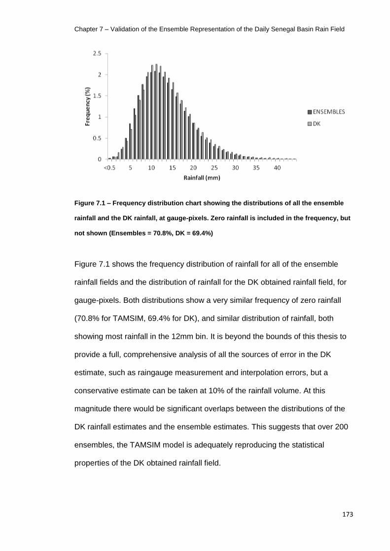
Chapter 7 – Validation of the Ensemble Representation of the Daily Senegal Basin Rain Field
173
Figure 7.1 – Frequency distribution chart showing the distributions of all the ensemble
rainfall and the DK rainfall, at gauge-pixels. Zero rainfall is included in the frequency, but
not shown (Ensembles = 70.8%, DK = 69.4%)
Figure 7.1 shows the frequency distribution of rainfall for all of the ensemble
rainfall fields and the distribution of rainfall for the DK obtained rainfall field, for
gauge-pixels. Both distributions show a very similar frequency of zero rainfall
(70.8% for TAMSIM, 69.4% for DK), and similar distribution of rainfall, both
showing most rainfall in the 12mm bin. It is beyond the bounds of this thesis to
provide a full, comprehensive analysis of all the sources of error in the DK
estimate, such as raingauge measurement and interpolation errors, but a
conservative estimate can be taken at 10% of the rainfall volume. At this
magnitude there would be significant overlaps between the distributions of the
DK rainfall estimates and the ensemble estimates. This suggests that over 200
ensembles, the TAMSIM model is adequately reproducing the statistical
properties of the DK obtained rainfall field.
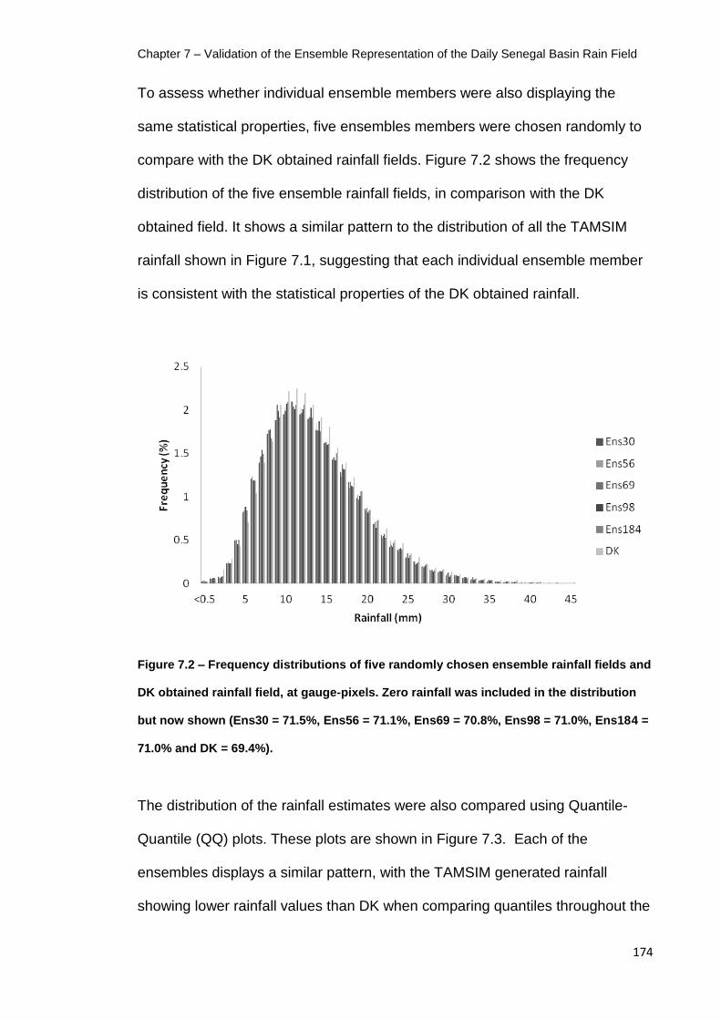
Chapter 7 – Validation of the Ensemble Representation of the Daily Senegal Basin Rain Field
174
To assess whether individual ensemble members were also displaying the
same statistical properties, five ensembles members were chosen randomly to
compare with the DK obtained rainfall fields. Figure 7.2 shows the frequency
distribution of the five ensemble rainfall fields, in comparison with the DK
obtained field. It shows a similar pattern to the distribution of all the TAMSIM
rainfall shown in Figure 7.1, suggesting that each individual ensemble member
is consistent with the statistical properties of the DK obtained rainfall.
Figure 7.2 – Frequency distributions of five randomly chosen ensemble rainfall fields and
DK obtained rainfall field, at gauge-pixels. Zero rainfall was included in the distribution
but now shown (Ens30 = 71.5%, Ens56 = 71.1%, Ens69 = 70.8%, Ens98 = 71.0%, Ens184 =
71.0% and DK = 69.4%).
The distribution of the rainfall estimates were also compared using Quantile-
Quantile (QQ) plots. These plots are shown in Figure 7.3. Each of the
ensembles displays a similar pattern, with the TAMSIM generated rainfall
showing lower rainfall values than DK when comparing quantiles throughout the

Chapter 7 – Validation of the Ensemble Representation of the Daily Senegal Basin Rain Field
175
plot. However, there is a close match between 10 and 25mm rainfall but a poor
match at the low and high end of the plots.
Figure 7.3 – QQ distribution plots showing DK and sample ensemble rainfall at gauge-
pixels.
Rainfall Characteristics at Catchment Average Scale
For use as an input driving the Pitman lumped CRR model, daily averages of
rainfall needed to be calculated from each ensemble member for the Bakoye

Chapter 7 – Validation of the Ensemble Representation of the Daily Senegal Basin Rain Field
176
catchment, as described in Chapter 5. The catchment average rainfall estimate
can be assessed by comparison with a catchment average determined from the
underlying DK rainfall field, and its skill can be compared with the deterministic
TAMSAT1 estimate, for all the ensembles together, individual ensemble
members, and a mean of all the ensemble estimates.
Figures 7.4 and 7.5 show the frequency distributions of rainfall at Bakoye
catchment scale, for TAMSIM, the five randomly selected ensemble members
and DK obtained rainfall. Interestingly, when averaged over the Bakoye
catchment scale, the proportion of zero rainfall is much lower for TAMSIM
generated rainfall fields (3.6%), than for DK obtained rainfall (19.3%). This is
caused by the amount of uncertainty for rainfall at CCD=0 in the TAMSIM
calibration – there is a 19% probability of rainfall at CCD=0, so even when the
whole Bakoye catchment shows CCD=0, it is likely that TAMSIM will estimate
rainfall somewhere within the catchment.

Chapter 7 – Validation of the Ensemble Representation of the Daily Senegal Basin Rain Field
177
Figure 7.4 – Frequency distribution showing the distributions of all the ensemble rainfall
fields and the DK obtained rainfall field, at the Bakoye catchment scale. Zero rainfall is
included in the distribution but not shown (Ensembles = 3.6%, DK = 19.3%).
Figure 7.5 – Frequency distribution of five randomly chosen ensemble rainfall fields and
DK obtained rainfall fields at Bakoye catchment scale. Zero rainfall is included in the
distribution but not shown (Ens30 = 3.7%, Ens56 = 4.0%, Ens69 = 3.5%, Ens98 = 3.0%,
Ens184 = 4.0%, DK = 19.3%).
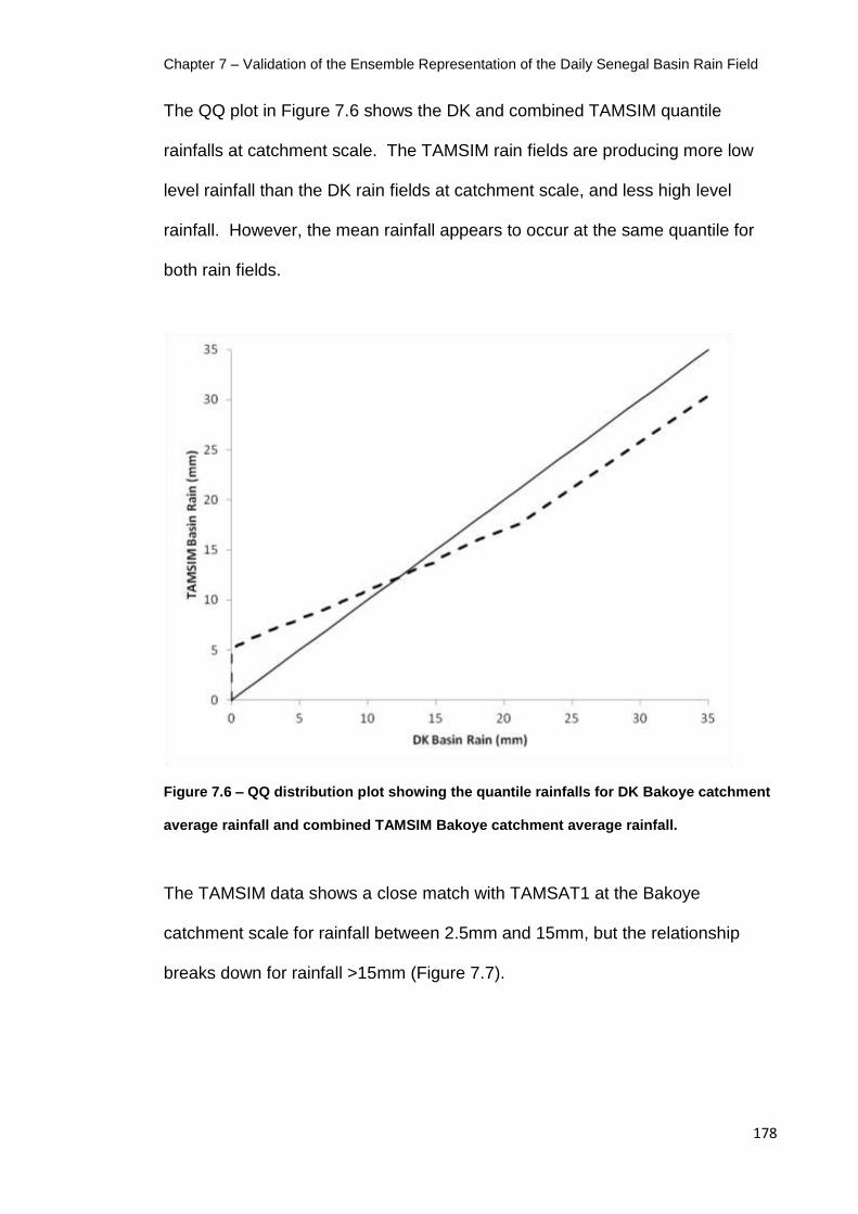
Chapter 7 – Validation of the Ensemble Representation of the Daily Senegal Basin Rain Field
178
The QQ plot in Figure 7.6 shows the DK and combined TAMSIM quantile
rainfalls at catchment scale. The TAMSIM rain fields are producing more low
level rainfall than the DK rain fields at catchment scale, and less high level
rainfall. However, the mean rainfall appears to occur at the same quantile for
both rain fields.
Figure 7.6 – QQ distribution plot showing the quantile rainfalls for DK Bakoye catchment
average rainfall and combined TAMSIM Bakoye catchment average rainfall.
The TAMSIM data shows a close match with TAMSAT1 at the Bakoye
catchment scale for rainfall between 2.5mm and 15mm, but the relationship
breaks down for rainfall >15mm (Figure 7.7).

Chapter 7 – Validation of the Ensemble Representation of the Daily Senegal Basin Rain Field
179
Figure 7.7 – QQ distribution plot showing the quantile rainfall for TAMSAT1 Bakoye
catchment average rainfall and TAMSIM Bakoye catchment average rainfall.
The ability of the TAMSIM algorithm to estimate rainfall at the catchment scale
can be compared to that of the deterministic TAMSAT1 estimate by using
measurements of relative skill, in comparison with the estimate produced by the
underlying DK daily rain field. Three skills scores were used for the quantitative
assessment, Root-Mean-Squared-Error (RMSE), the coefficient of
determination (R2), and Bias (BIAS), as defined below:
Equation 7.1

Chapter 7 – Validation of the Ensemble Representation of the Daily Senegal Basin Rain Field
180
Equation 7.2
Equation 7.3
where is the number of daily rainfall estimates in the dataset, is the DK
daily catchment rainfall estimate, is the SRFE daily catchment rainfall
estimate (either TAMSAT1, or TAMSIM) and is the mean of the DK daily
catchment rainfall estimates.
The skill scores were applied to the TAMSAT1 estimate, the collective of
TAMSIM ensemble estimates (SIMAll) and the mean of the ensemble estimates
(SIMMean), for the period between 1986 and 1996, and for each individual year
between. The results can be seen in Table 7.1.

Chapter 7 – Validation of the Ensemble Representation of the Daily Senegal Basin Rain Field
181
Period Method RMSE R2 BIAS
All TAMSAT1 3.94 0.31 0.34 SIMAll 4.59 0.51 0.41
SIMMean 3.94 0.31 0.41
1986 TAMSAT1 3.89 0.36 0.64 SIMAll 4.57 0.56 0.68 SIMMean 3.94 0.35 0.68
1987 TAMSAT1 3.60 0.38 -0.30 SIMAll 4.31 0.64 -0.25 SIMMean 3.62 0.37 -0.25
1988 TAMSAT1 4.39 0.34 0.52 SIMAll 5.04 0.52 0.61 SIMMean 4.40 0.34 0.61
1989 TAMSAT1 4.45 0.33 0.89 SIMAll 4.97 0.49 0.92 SIMMean 4.41 0.33 0.92
1990 TAMSAT1 2.91 0.38 -0.31 SIMAll 3.78 0.64 -0.25 SIMMean 2.91 0.37 -0.25
1991 TAMSAT1 3.85 0.28 0.22 SIMAll 4.48 0.49 0.30 SIMMean 3.81 0.28 0.30
1992 TAMSAT1 3.71 0.31 -0.38 SIMAll 4.33 0.54 -0.27 SIMMean 3.66 0.30 -0.27
1993 TAMSAT1 3.64 0.28 0.11 SIMAll 4.29 0.51 0.16 SIMMean 3.63 0.27 0.16
1994 TAMSAT1 4.59 0.35 1.01 SIMAll 5.19 0.57 1.06 SIMMean 4.60 0.35 1.06
1995 TAMSAT1 3.90 0.31 0.57 SIMAll 4.61 0.49 0.66 SIMMean 3.94 0.31 0.66
1996 TAMSAT1 4.14 0.23 0.77 SIMAll 4.75 0.39 0.85 SIMMean 4.16 0.24 0.85
Table 7.1 – Table showing comparison skill scores for Bakoye catchment rainfall
estimates from TAMSAT1, all of the TAMSIM ensembles (SIMAll), and the mean of the
TAMSIM ensembles (SIMMean), the whole 11 year study period, and for individual years
(wet season data only).
The skill scores shown in Table 7.1 portray a mixed picture. In terms of R2, the
TAMSIM ensembles outperform the TAMSAT1 estimate, but TAMSAT1 shows
a better fit in terms of RMSE and less bias, for the whole 11 year period.
Generally, and as would be expected, the mean of the TAMSIM ensembles
shows similar error scores to TAMSAT1, and the same bias as the whole
TAMSIM ensemble estimates. In regards to bias, overall the SRFE slightly

Chapter 7 – Validation of the Ensemble Representation of the Daily Senegal Basin Rain Field
182
underestimates in comparison with the DK estimate, but overestimates in
1987,1990 and 1992 – each anomalously dry years.
Reliability of Ensemble Estimates
The reliability of ensemble estimates can be assessed using the forecast
reliability method detailed by Toth et al. (2003). The reliability plots use a
threshold on the ensemble data, and bins the data for each day into percentage
of ensemble members above the threshold. For each bin the percentage of
days that show recorded data above the threshold is calculate and plotted
against the binned ensemble data. A reliable ensemble set will show a 1:1
relationship on the plot, for example if 40% of ensembles estimate rainfall above
5mm, than there should be a 40% chance of rainfall occurring above 5mm on
that day.
Figure 7.8 shows reliability plots for the catchment average TAMSIM SRFE,
compared to the DK catchment average rainfall estimate, for three threshold
levels – low rainfall (25th percentile from the DK rain), mean rainfall and high
level rainfall (75th percentile). The TAMSIM ensembles show good reliability at
mean and high level rainfall, but poor reliability at the low level rainfall threshold
– this is most likely due to the known problem that SRFE have with estimating
trace levels of rainfall.
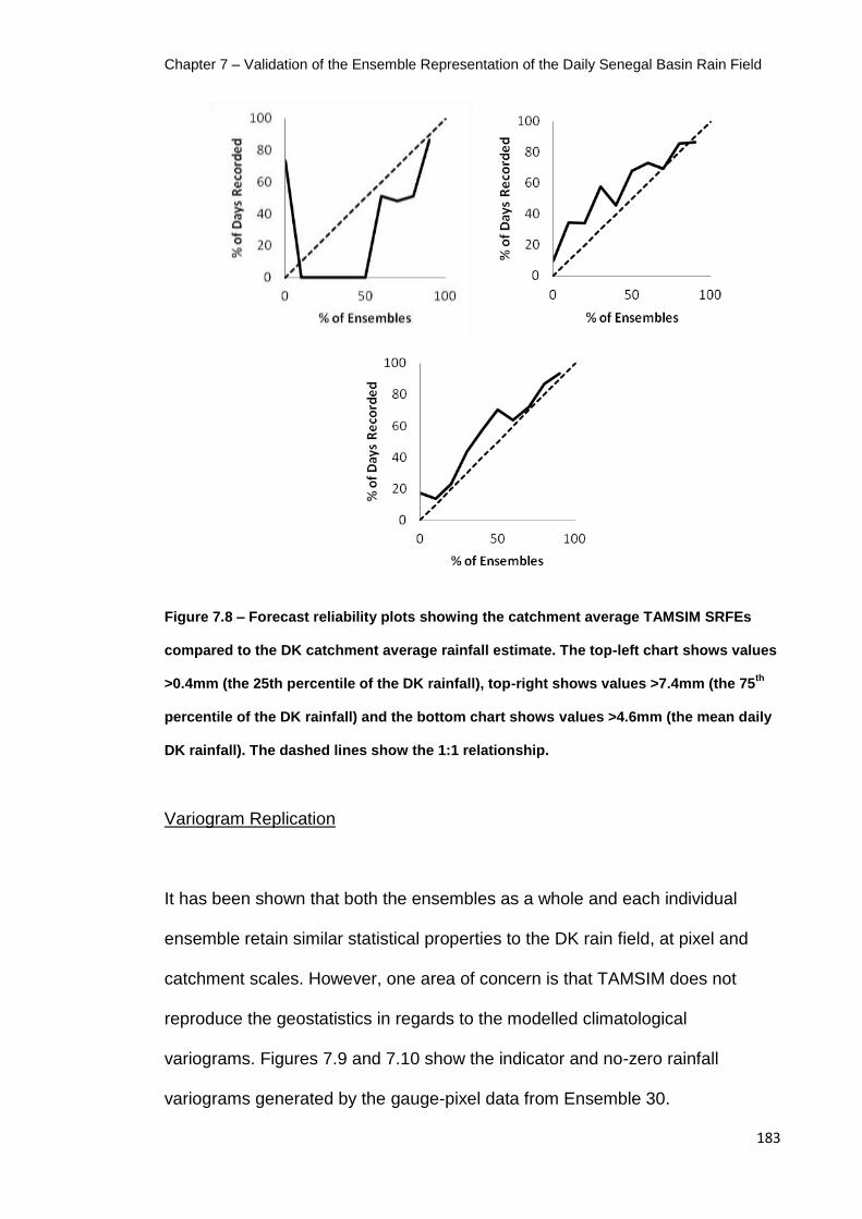
Chapter 7 – Validation of the Ensemble Representation of the Daily Senegal Basin Rain Field
183
Figure 7.8 – Forecast reliability plots showing the catchment average TAMSIM SRFEs
compared to the DK catchment average rainfall estimate. The top-left chart shows values
>0.4mm (the 25th percentile of the DK rainfall), top-right shows values >7.4mm (the 75th
percentile of the DK rainfall) and the bottom chart shows values >4.6mm (the mean daily
DK rainfall). The dashed lines show the 1:1 relationship.
Variogram Replication
It has been shown that both the ensembles as a whole and each individual
ensemble retain similar statistical properties to the DK rain field, at pixel and
catchment scales. However, one area of concern is that TAMSIM does not
reproduce the geostatistics in regards to the modelled climatological
variograms. Figures 7.9 and 7.10 show the indicator and no-zero rainfall
variograms generated by the gauge-pixel data from Ensemble 30.

Chapter 7 – Validation of the Ensemble Representation of the Daily Senegal Basin Rain Field
184
Figure 7.9 – Modelled wet-season climatological ‘indicator’ variogram generated from
Ens30 gauge-pixel data.
Figure 7.10 – Modelled wet-season climatological ‘no-zero’ variogram generated from
Ens30 gauge-pixel data.

Chapter 7 – Validation of the Ensemble Representation of the Daily Senegal Basin Rain Field
185
The two modelled variograms shown in Figures 7.9 and 7.10 show little
resemblance to the modelled variograms shown for the DK in Chapter 4,
derived directly from the raingauge data. Table 7.2 and 7.3 compare the
parameters between the modelled variograms for the DK rain fields, the residual
variograms used for TAMSIM, and the variograms generated from each of the
sample ensemble members.
Nugget Sill Range (km)
From Gauges 0.37 0.71 183.02
Residual 0.00 1.27 146.15
Ens30 0.09 1.03 112.52
Ens56 0.09 1.02 113.30
Ens69 0.07 1.04 110.57
Ens98 0.10 1.03 117.27
Ens184 0.10 1.02 112.92
Table 7.2 – Table showing the modelled ‘indicator’ variogram parameters for variograms
from the gauges, the residual variogram, and variograms generated from the sample
ensemble members.

Chapter 7 – Validation of the Ensemble Representation of the Daily Senegal Basin Rain Field
186
Nugget Sill Range (km)
From Gauges 0.50 0.51 50.79
Residual 0.00 1.16 92.56
Ens30 0.11 1.06 105.30
Ens56 0.04 1.12 100.60
Ens69 0.05 1.11 101.64
Ens98 0.07 1.11 106.71
Ens184 0.09 1.09 109.80
Table 7.3 – Table showing the modelled ‘no-zero’ variogram parameters for variograms
from the gauges, the residual variograms, and variograms generated from the sample
ensemble members.
From Tables 7.2 and 7.3 it can be seen that the variogram parameters for each
of the sample ensemble members are relatively consistent. Both the indicator
and the no-zero variograms for the Ensemble members also show a low
nugget, much lower than the gauge derived variograms. The Ensemble
variograms also show greater similarity to the residual variogram, especially in
the case of the no-zero transforms, and this is not unexpected as the residual
variogram is used directly in the generation of the variograms. However, it is of
concern that each individual ensemble rain field does not reproduce a
variogram more reflective of the geostatistics shown by the raingauges – this is
most likely a result of TAMSIM being unable to reproduce the rainfall gradient
across the region using a single calibration.

Chapter 7 – Validation of the Ensemble Representation of the Daily Senegal Basin Rain Field
187
7.3 – Influence of Uncertainty on the Estimates
The sections above have demonstrated the ability of the TAMSIM algorithm to
reproduce the rainfall characteristics of the daily Senegal rainfall field, at both
gauge-pixel and catchment average scale. It has been previously stated that the
types of uncertainty with a SRFE are likely to emerge from errors in estimating
where it is raining, when it is raining, and the rainfall rate. These can be
observed in the ensemble estimates as spatial biases and temporal biases, in
addition to error.
Spatial Bias
The spatial biases within the TAMSIM ensemble estimates can be seen by
observing the rainfall distributions at gauge-pixel scale for individual raingauges.
In order to show this, five raingauges were randomly selected from the whole
record and the TAMSIM pixel rainfall for each gauge compared to the DK
obtained pixel average for that gauge – the frequency distributions shown in
Figure 7.11 to 7.15, with the raingauges ordered from most northerly to most
southerly.

Chapter 7 – Validation of the Ensemble Representation of the Daily Senegal Basin Rain Field
188
Figure 7.11 – Frequency distribution of TAMSIM rainfall fields and DK obtained rainfall for
the Aero-Lao gauge-pixel. Zero rainfall is included in the distribution but not shown
(TAMSIM = 76.2%, DK = 91.1%).
Figure 7.12 – Frequency distribution of TAMSIM rainfall fields and DK obtained rainfall for
the Renerou gauge-pixel. Zero rainfall is included in the distribution but not shown
(TAMSIM = 74.3%, DK = 81.6%).

Chapter 7 – Validation of the Ensemble Representation of the Daily Senegal Basin Rain Field
189
Figure 7.13 – Frequency distribution of TAMSIM rainfall fields and DK obtained rainfall for
the Thiel gauge-pixel. Zero rainfall is included in the distribution but not shown (TAMSIM
= 74.3%, DK = 84.3%).
Figure 7.14 – Frequency distribution of TAMSIM rainfall fields and DK obtained rainfall for
the Guene-Gore gauge-pixel. Zero rainfall is included in the distribution but not shown
(TAMSIM = 67.7%, DK = 63.4%).

Chapter 7 – Validation of the Ensemble Representation of the Daily Senegal Basin Rain Field
190
Figure 7.15 – Frequency distribution of TAMSIM rainfall fields and DK obtained rainfall for
the Oualia gauge-pixel. Zero rainfall is included in the distribution but not shown
(TAMSIM = 65.1%, DK = 50.0%).
It can be seen from Figures 7.11 to 7.15 that the TAMSIM rainfall fields do not
recreate the rainfall statistics at individual gauge-pixel level. However, this
manifests itself differently for each gauge, for example at the Aero-Lao gauge-
pixel (in the drier, northern part of the Senegal Basin), TAMSIM overestimates
the distribution of rainfall with the DK rainfall estimate showing a greater
proportion of zero rainfall (TAMSIM = 76.2%, DK = 91.1%). In contrast, for the
Oualia gauge-pixel (in the wetter, southern part of the Senegal Basin), TAMSIM
underestimates the rainfall distribution, with the DK estimate showing less zero
rainfall (TAMSIM = 65.1%, DK = 50.0%). This same north to south variation
can be observed by comparing the QQ plots for the sample gauge-pixels
(Figure 7.16).

Chapter 7 – Validation of the Ensemble Representation of the Daily Senegal Basin Rain Field
191
Figure 7.16 – QQ distribution plots showing quantile rainfall at sample gauge-pixels for
DK rain fields and combined TAMSIM rain fields.
The QQ plots in Figure 7.16 show that out of the sample gauge-pixels, the
Guene-Gore pixel shows the best match between the TAMSIM quantile rainfalls

Chapter 7 – Validation of the Ensemble Representation of the Daily Senegal Basin Rain Field
192
and the DK quantile rainfalls. This matches the distributions of rainfall shown in
Figure 7.11 to 7.15.
The reliability of the ensembles can also be observed at gauge-pixel scale,
using the TAMSIM ensemble and DK data from pixels containing the selected
raingauge stations used previously. The reliability plots for these are shown in
Figures 7.17 to 7.21, ordered from most northerly to most southerly. Along with
each reliability plot is a bar chart showing the number of samples in each bin,
the low number of samples for the 40, 50, 90 and 100% bins generally contain
very few samples and this causes a lot of the noise in the charts.
Figure 7.17 – Forecast reliability plots showing the TAMSIM SRFE compared to the DK
catchment average rainfall estimate for the pixel containing the Aero-Lao raingauge
station. The chart shows values >1.4mm (the mean daily DK rainfall). The dashed lines
show the 1:1 relationship. The bar chart on the right shows the number of samples in
each bin.

Chapter 7 – Validation of the Ensemble Representation of the Daily Senegal Basin Rain Field
193
Figure 7.18 – Forecast reliability plots showing the TAMSIM SRFE compared to the DK
catchment average rainfall estimate for the pixel containing the Renerou raingauge
station. The chart shows values >2.7mm (the mean daily DK rainfall). The dashed lines
show the 1:1 relationship. The bar chart on the right shows the number of samples in
each bin.
Figure 7.19 – Forecast reliability plots showing the TAMSIM SRFE compared to the DK
catchment average rainfall estimate for the pixel containing the Thiel raingauge station.
The chart shows values >2.2mm (the mean daily DK rainfall). The dashed lines show the
1:1 relationship. The bar chart on the right shows the number of samples in each bin.

Chapter 7 – Validation of the Ensemble Representation of the Daily Senegal Basin Rain Field
194
Figure 7.20 – Forecast reliability plots showing the TAMSIM SRFE compared to the DK
catchment average rainfall estimate for the pixel containing the Guene-Gore raingauge
station. The chart shows values >5.3mm (the mean daily DK rainfall). The dashed lines
show the 1:1 relationship. The bar chart on the right shows the number of samples in
each bin.
Figure 7.21 – Forecast reliability plots showing the TAMSIM SRFE compared to the DK
catchment average rainfall estimate for the pixel containing the Oualia raingauge station.
The chart shows values >7.1mm (the mean daily DK rainfall). The dashed lines show the
1:1 relationship. The bar chart on the right shows the number of samples in each bin.
The reliability plots of Figures 7.17 to 7.21 demonstrate how the heterogeneity
of the Senegal Basin area influences the reliability of the TAMSIM ensembles,
clearly showing that the relationship between CCD and rainfall is non-stationary
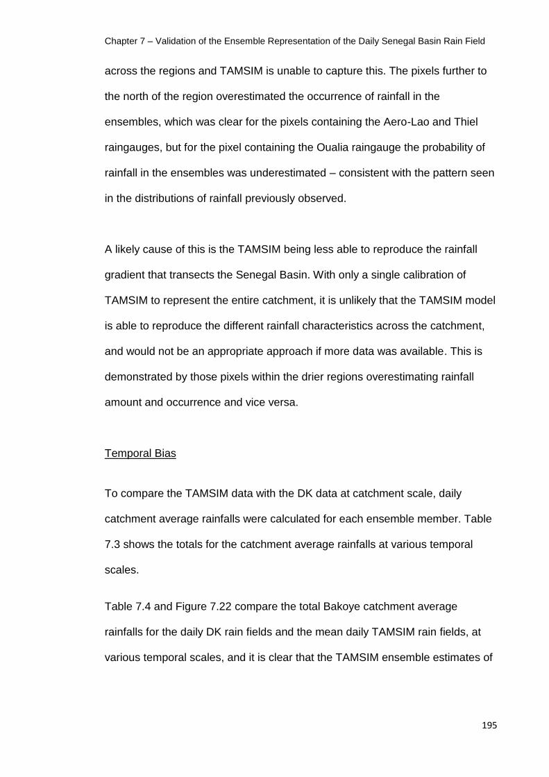
Chapter 7 – Validation of the Ensemble Representation of the Daily Senegal Basin Rain Field
195
across the regions and TAMSIM is unable to capture this. The pixels further to
the north of the region overestimated the occurrence of rainfall in the
ensembles, which was clear for the pixels containing the Aero-Lao and Thiel
raingauges, but for the pixel containing the Oualia raingauge the probability of
rainfall in the ensembles was underestimated – consistent with the pattern seen
in the distributions of rainfall previously observed.
A likely cause of this is the TAMSIM being less able to reproduce the rainfall
gradient that transects the Senegal Basin. With only a single calibration of
TAMSIM to represent the entire catchment, it is unlikely that the TAMSIM model
is able to reproduce the different rainfall characteristics across the catchment,
and would not be an appropriate approach if more data was available. This is
demonstrated by those pixels within the drier regions overestimating rainfall
amount and occurrence and vice versa.
Temporal Bias
To compare the TAMSIM data with the DK data at catchment scale, daily
catchment average rainfalls were calculated for each ensemble member. Table
7.3 shows the totals for the catchment average rainfalls at various temporal
scales.
Table 7.4 and Figure 7.22 compare the total Bakoye catchment average
rainfalls for the daily DK rain fields and the mean daily TAMSIM rain fields, at
various temporal scales, and it is clear that the TAMSIM ensemble estimates of

Chapter 7 – Validation of the Ensemble Representation of the Daily Senegal Basin Rain Field
196
rainfall are not able to reflect fully the interannual variations of rainfall in the
same way as the DK estimate.
DK Rain (mm) TAMSIM Mean Rain (mm)
Total 7798.91 7116.43
Mean 708.99 646.95
1986 726.77 623.46
1987 595.34 633.14
1988 805.87 712.89
1989 772.00 630.76
1990 637.99 675.50
1991 683.09 637.74
1992 598.98 640.83
1993 635.16 610.81
1994 851.95 690.01
1995 763.98 663.51
1996 727.78 597.77
Table 7.4 – Table showing the total catchment average rainfall, mean annual catchment
average rainfall and yearly wet-season totals for DK and TAMSIM mean daily rain fields.

Chapter 7 – Validation of the Ensemble Representation of the Daily Senegal Basin Rain Field
197
Figure 7.22 – Chart showing the annual Bakoye catchment average rainfall totals for the
wet seasons of 1986-1996, for the DK daily rain fields and the mean TAMSIM daily rain
fields.
If it is assumed that the bias calculated for the TAMSIM ensemble estimates for
the whole 11 year study period is a result of spatial bias, it is possible to adjust
the bias for each wet season to remove the influence of the spatial bias –
leaving the systematic bias during years of anomalous rainfall. Figure 7.23
shows the bias anomalies for each wet season in the record and it is clear that it
shows a similar pattern to the rainfall anomalies seen in the raingauge data, as
shown in Figure 3.17.

Chapter 7 – Validation of the Ensemble Representation of the Daily Senegal Basin Rain Field
198
Figure 7.23 – Chart showing the bias anomalies for each wet season, as deviated from
the BIAS calculated for the whole 11 year study period, for the TAMSIM ensemble
catchment average rainfall estimates.
7.4 – Conclusions
The Senegal Basin daily rainfall fields, produced by the TAMSIM algorithm have
been analysed at various spatial and temporal scales, including at gauge-pixels
and catchment scales. The ensemble estimates of rainfall have been assessed
as a collective, from a sample individual ensemble members, and as a mean of
all the members. At catchment scale, the algorithm’s performance has been
directly compared to a deterministic estimate of rainfall produced by the
TAMSAT1 method.
-0.8
-0.6
-0.4
-0.2
0
0.2
0.4
0.6
0.8
1986 1987 1988 1989 1990 1991 1992 1993 1994 1995 1996
TAM
SIM
BIA
S A
no
mal
y (m
m)

Chapter 7 – Validation of the Ensemble Representation of the Daily Senegal Basin Rain Field
199
Overall, the algorithm has performed well in estimating the daily rainfall field, for
both the collective of the ensembles and for each individual ensemble member.
The distribution of rainfall values closely matches that estimated by the DK rain
field at both gauge-pixel and catchment scale. These relationships are
replicated when looking at individual ensemble members.
Of particular note from the results is the systematic biases that exist within the
SRFE, when compared to the DK gauges based rainfall estimation. Teo (2006)
noted that TAMSAT1 and TAMSIM both showed biases for years with
anomalous rainfall, and this is also evident with the data for the Senegal Basin.
In all there are four types of bias that can be said to exist in the data:
1. Overall bias – both TAMSAT1 and TAMSIM are shown to estimate lower
volumes of rainfall than the underlying DK rain field, but are
indistinguishable within the bounds of conservative error estimates.
2. Bias due to local variations in rainfall – there are biases in the catchment
rainfall estimates for the Bakoye catchment due to local variations in
rainfall, in respect to the overall Senegal Basin from which the calibration
is derived.
3. Bias due to intraseason variations – it is clear that the relationship
between CCD and rainfall is not stationary over the wet season and
these variations will result in biased estimates for periods where the
relationship has altered.

Chapter 7 – Validation of the Ensemble Representation of the Daily Senegal Basin Rain Field
200
4. Bias due to interannual variations – the majority of the years in the study
period do not demonstrate rainfall close to the mean for the period, and
for these years there exists systematic bias in the estimates. The SRFE
overestimates rainfall for dry years and vice versa.
The bias resulting from sources 2 and 3 are particularly marked in this thesis
due to the paucity of raingauge data available. With a denser network it would
have been possible to focus the calibration of the SRFE on data collected in
and around the Bakoye catchment. With a denser network it would have been
possible to use finer temporal resolutions for calibrations, such as the monthly
calibrations adopted by Teo (2006) and Teo and Grimes (2007). Greatrex
(2012) demonstrated how regional calibrations could be adopted into the
method, subdividing the region into fairly homogenous zones and calibrating
separately for each but still producing a single rainfall field. The addition of more
extensive ground data in the manner above would reduce the biases, possibly
significantly so, but not remove it completely – thus it is important to understand
how the bias in the SRFE propagates to downstream applications.
The systematic bias caused by interannual variations of rainfall deviating from
the mean over the calibration period may be reduced somewhat with additional
ground data, but as it was evident in the study by Teo (2006) it is likely to be
significant even for areas with a dense network. To reduce this it is likely that an
additional data set would be required, such as sea surface temperature (SST)
would need to be incorporated into the study – this is discussed in Chapter 10.

Chapter 7 – Validation of the Ensemble Representation of the Daily Senegal Basin Rain Field
201
For production of daily catchment estimates of rainfall - which will be used to
drive the Pitman lumped CRR model - the TAMSIM estimates performed
favourably compared to the TAMSAT1 showing a better fit in regards to the R2
score.
Chapter 8 demonstrates how the catchment averages of the TAMSIM ensemble
SRFE can be used to show the propagation of the uncertainty through the
Pitman lumped CRR model, and showing how a fully spatio-temporally
distributed stochastic ensemble approach is superior to a simpler perturbation
method for this application.

Chapter 8 – The Influence of SRFE Input Uncertainty on Hydrological Model Output
202
8 The Influence of SRFE Input
Uncertainty on Hydrological Model
Output
8.1 – Introduction
Chapter 7 demonstrated how significant uncertainties exist within the TAMSAT1
satellite rainfall estimate (SRFE) of the daily rain fields for the Senegal Basin.
These uncertainties have been characterised and represented by an ensemble
of 200 unique yet equiprobable rainfall estimates using the TAMSIM algorithm,
from which catchment averages were calculated for use as an input in a lumped
conceptual rainfall-runoff (CRR) model. The lumped CRR model used was the
Pitman model calibrated using the Shuffled Complex Evolution (SCE-UA)
method - details of both can be seen in Chapter 6.
The use of ensemble representations of uncertainty allows for a simple way of
representing the uncertainty in the input, as each can be used as an individual
estimate of the rainfall and applied in turn as a rainfall input in the model. The

Chapter 8 – The Influence of SRFE Input Uncertainty on Hydrological Model Output
203
distribution of the ensemble of modelled outputs, in this case discharges, can
be said to show the bounds of uncertainty of the output with regard to the input
uncertainty. However, the influence of uncertainty within the hydrological model
itself, in particular in the form of model structure and parameter uncertainty, and
the way that the SRFE uncertainty interacts with them, cannot be ignored. To
this end, before the influence of the uncertainty within a SRFE can be measured
propagating through the Pitman model a suitable set of parameter values must
be established for use with ensemble inputs.
The EnsAll parameterisation is introduced as a new method for calibrating a
deterministic hydrological model for use with ensemble rainfall inputs. The
method incorporates each ensemble member in turn - looping the recorded
discharge data and resetting the initial conditions at the end of each 11 year
period. This method of parameterisation was shown to outperform all the
alternative methods, with little overall bias, and showed similar levels of
performance when compared to outputs from calibrations against each
individual ensemble input.
This chapter addresses three of the key research questions outlined in Chapter
1. Section 8.2 details the performance of the Pitman model driven by the
TAMSIM ensemble rainfall estimates when calibrated by different rainfall
estimates, showing that a calibration method that incorporates each of the
TAMSIM ensemble estimates (EnsAll) is the most favourable option. Section
8.3 describes in detail the performance of the Pitman model using the EnsAll
parameterisation, detailing the envelope hydrographs representing the

Chapter 8 – The Influence of SRFE Input Uncertainty on Hydrological Model Output
204
propagation of the uncertainty as shown by the TAMSIM ensemble SRFE,
demonstrating that biases within the SRFE are directly passed on resulting in
biases in the discharge output. Section 8.4 will demonstrate how the TAMSIM
ensemble SRFE are superior in representing the full range of input uncertainty
when compared to a simpler perturbation approach. Finally, Section 8.5
concludes the chapter.
8.2 – Ensemble Parameterisation of the Pitman Model
The Pitman lumped CRR model is a deterministic model, which is designed to
operate when driven by a single rainfall input, and models a single discharge
output for each timestep. For calibration using the SCE-UA algorithm a
deterministic estimate of rainfall is required to drive the Pitman model, whilst the
parameter values are adjusted to match the deterministic output against the
recorded discharge data. The TAMSIM approach to characterising SRFE
uncertainty produces a group of ensemble rainfall inputs that each resemble a
deterministic input that can be used to drive the Pitman model, and although a
parameter set can be produced for each individual ensemble this is not
appropriate for operational purposes, especially if ensemble inputs are to be
used to forecast discharges. There is a requirement to determine a single
parameter set that can be said to be optimal for the data, and transferable
between the ensembles and temporal periods.
The Pitman model was calibrated against several available deterministic
estimates of rainfall using SCE-UA, and each calibrated parameter set is

Chapter 8 – The Influence of SRFE Input Uncertainty on Hydrological Model Output
205
referred to as a parameterisation henceforth when used with the TAMSIM
ensemble estimates:
EnsStart – Calibration of the Pitman model provided by David Grimes
(personal correspondence, 2009). This parameter set was also used as
the initial parameter set in the SCE-UA calibrations.
EnsGA – Calibration against the Gauge Average estimate (an area
weighted estimate using a Thiessen Polygons method with an
adjustment for orographic effects).
EnsDK – Calibration against the catchment average of the DK rainfall.
EnsTAM1 – Calibration against the TAMSAT1 estimate.
In addition to the deterministic estimates the Pitman model was calibrated using
rainfall inputs using the Bakoye catchment average TAMSIM ensemble
estimates:
EnsMean – Calibration against the daily mean of the 200 TAMSIM
ensemble estimates.
EnsAll – Calibration against each of the 200 TAMSIM ensemble
members in turn, effectively a 2,200 year record with the recorded
discharge looped and the stores reset to 0 at the end of each 11year
period.
The relative performance of each parameterisation when driven by the TAMSIM
ensemble estimates can be seen in Figure 8.1. It is evident that the EnsAll

Chapter 8 – The Influence of SRFE Input Uncertainty on Hydrological Model Output
206
calibration displays the best performance, with a mean RMSE of 133.91% of the
mean daily recorded discharge. Both the EnsMean and EnsTAM1
parameterisation show poor transferability when driven by different TAMSIM
ensemble estimates, which is most likely a result of overparameterisation.
Figure 8.1 – Chart showing the relative performances for different parameterisations of
the Pitman model, when driven by the TAMSIM ensemble estimates for the Bakoye
catchment, 1986-1996.
The influence of the parameterisation of the modelling of discharge can be seen
in Figure 8.2, which compares the EnsAll and EnsMean outputs for the 1992
wet season.

Chapter 8 – The Influence of SRFE Input Uncertainty on Hydrological Model Output
207
Figure 8.2 – Envelope hydrographs showing the modelled discharges for the 1992 wet
season, from both the EnsMean (red) and the EnsAll (blue) parameterisation. The
TAMSAT1 deterministic discharge is shown by the dashed green line. The envelopes
show the 95% confidence bounds from the modelled discharges.
From Figure 8.2 it is clear that the EnsMean modelled discharges do not show a
good representation of the propagation of the SRFE uncertainty as it
propagates through the Pitman model, as the parameter uncertainty within the
Pitman model is high and interacting with the input uncertainty to produce a
wide envelope of modelled discharges. For the late wet season the EnsMean
discharges become entirely uncoupled from the TAMSAT1 deterministic
estimate. A similar pattern is seen for each year of the record.
To assess the performance of each parameterisation when the Pitman model is
driven by the TAMSIM ensemble estimates, the Pitman model was calibrated
using each ensemble individually. The collected output from the 200
0
200
400
600
800
1000
1200
1400
6/1/1992 7/1/1992 8/1/1992 9/1/1992 10/1/1992 11/1/1992 12/1/1992
Dis
char
ge (
cum
ecs
)

Chapter 8 – The Influence of SRFE Input Uncertainty on Hydrological Model Output
208
parameterisations is referred to as EnsInd and is used as a proxy for the
optimal model. Table 8.1 shows performance statistics for each of the
parameterisation methods derived from the SRFE.
Calibration
Regime RMSE (%) R2 BIAS (%)
1986-1996
EnsTAM1 114.42 1.10 24.34
EnsInd 85.65 0.57 3.83
EnsMean 116.68 1.63 -163.61
EnsAll 89.08 0.52 0.80
Table 8.1 – Table showing performance statistics for the parameterisations derived from
the SRFE, comparing them to the EnsInd output. The table shows values for wet season
data only. RMSE and BIAS shown as percentages of the mean daily discharge for the
period.
The values in Table 8.1 show that the Pitman model performs best when
calibrated to each individual ensemble, as in EnsInd, although the performance
of the EnsAll model is similar. EnsAll actually shows a less biased output than
the EnsInd output over the 11 years of the study period. EnsTAM1 and
EnsMean both perform very poorly and display high biases.
8.3 – The Propagation of Input Uncertainty through the Pitman
Model
The previous section analysed the available parameterisations that can be used
for the Pitman model when driven by the TAMSIM ensemble estimates,
showing that calibrations against deterministic estimates based on the SRFE
are not suitable for this purpose. The EnsAll parameterisation incorporates each

Chapter 8 – The Influence of SRFE Input Uncertainty on Hydrological Model Output
209
individual ensemble member in a single record and provides a robust calibration
of the Pitman model, which outperforms each of the alternative methods. EnsAll
was also shown to be comparable to the optimal proxy, EnsInd.
With the EnsAll parameterisation shown to be the optimal method available it
can be used to model the envelope hydrographs for each year of the record,
displaying the 95% confidence discharge envelope of the modelled discharges
between the 2.5th percentile and the 97.5th percentile for each day. These are
shown in Figures 8.3 to 8.13.
Figure 8.3 – Hydrograph showing the 95% confidence discharge envelope (in red) for
1986 for the Bakoye Catchment, driven by the TAMSIM ensemble SRFE using the EnsAll
parameterisation. The solid blue line shows the deterministic TAMSAT1 discharge, and
the dashed line shows the recorded discharge. (Note – 1986 represents the first year of
the modelling and is therefore subject to the ‘charging period’)
Figure 8.3 shows the 95% confidence discharge envelope for the 1986 wet
season for the period 1986-1996. Due to the nature of the dry season in the
region there appears to be little influence of a charging period in the

Chapter 8 – The Influence of SRFE Input Uncertainty on Hydrological Model Output
210
hydrograph, and the TAMSAT1 estimate (blue line) closely follows the recorded
discharge (dashed black line). Between July and October the discharge
envelope roughly lies equally above and below the TAMSAT1 estimate, but
TAMSAT1 becomes decoupled after October dropping to the lower end of the
envelope. From the raingauges 1986 displayed rainfall close to the mean for the
period, 592.95mm and 607.83mm respectively. The discharge from the
TAMSAT1 and TAMSIM estimates show little bias.
Figure 8.4 – Hydrograph showing the 95% confidence discharge envelope (in red) for
1987 for the Bakoye Catchment, driven by the TAMSIM ensemble SRFE using the EnsAll
parameterisation. The solid blue line shows the deterministic TAMSAT1 discharge, and
the dashed line shows the recorded discharge.
The raingauges in 1987 showed rainfall below the mean for the period for the
Senegal Basin region. For the gauges associated with the Bakoye catchment
this was particularly significant, with rainfall 150mm below the mean for the
year, being the driest year in the record. The hydrograph shows significant bias,
the Pitman model overestimating the discharge throughout the wet season. The

Chapter 8 – The Influence of SRFE Input Uncertainty on Hydrological Model Output
211
bias is such that most of the recorded discharge is below the bounds of the
modelled uncertainty.
Figure 8.5 – Hydrograph showing the 95% confidence discharge envelope (in red) for
1988 for the Bakoye Catchment, driven by the TAMSIM ensemble SRFE using the EnsAll
parameterisation. The solid blue line shows the deterministic TAMSAT1 discharge, and
the dashed line shows the recorded discharge.

Chapter 8 – The Influence of SRFE Input Uncertainty on Hydrological Model Output
212
Figure 8.6 – Hydrograph showing the 95% confidence discharge envelope (in red) for
1989 for the Bakoye Catchment, driven by the TAMSIM ensemble SRFE using the EnsAll
parameterisation. The solid blue line shows the deterministic TAMSAT1 discharge, and
the dashed line shows the recorded discharge.
Both 1988 and 1989, shown in Figures 8.5 and 8.6, displayed above average
rainfall to similar degrees. This was more significant in the Bakoye catchment
gauges. The deterministic and ensemble modelled discharges show little bias,
with 1988 being a particularly close match with the recorded discharge, yet the
timing of the peak discharge in the 1989 wet season is late.

Chapter 8 – The Influence of SRFE Input Uncertainty on Hydrological Model Output
213
Figure 8.7 – Hydrograph showing the 95% confidence discharge envelope (in red) for
1990 for the Bakoye Catchment, driven by the TAMSIM ensemble SRFE using the EnsAll
parameterisation. The solid blue line shows the deterministic TAMSAT1 discharge, and
the dashed line shows the recorded discharge.
Figure 8.8 – Hydrograph showing the 95% confidence discharge envelope (in red) for
1991 for the Bakoye Catchment, driven by the TAMSIM ensemble SRFE using the EnsAll
parameterisation. The solid blue line shows the deterministic TAMSAT1 discharge, and
the dashed line shows the recorded discharge.

Chapter 8 – The Influence of SRFE Input Uncertainty on Hydrological Model Output
214
Figure 8.9 – Hydrograph showing the 95% confidence discharge envelope (in red) for
1992 for the Bakoye Catchment, driven by the TAMSIM ensemble SRFE using the EnsAll
parameterisation. The solid blue line shows the deterministic TAMSAT1 discharge, and
the dashed line shows the recorded discharge.
Figure 8.10 – Hydrograph showing the 95% confidence discharge envelope (in red) for
1993 for the Bakoye Catchment, driven by the TAMSIM ensemble SRFE using the EnsAll
parameterisation. The solid blue line shows the deterministic TAMSAT1 discharge, and
the dashed line shows the recorded discharge.

Chapter 8 – The Influence of SRFE Input Uncertainty on Hydrological Model Output
215
Figure 8.7 to 8.10 show the hydrographs for the period 1990 to 1993, a period
that displayed consistently below average rainfall for both the whole Senegal
Basin area and the Bakoye catchment. There is some bias evident in 1990, with
an overestimation of the discharge by the models, but a close match with the
recorded discharge for the rest of the years in this dry period.
Figure 8.11 – Hydrograph showing the 95% confidence discharge envelope (in red) for
1994 for the Bakoye Catchment, driven by the TAMSIM ensemble SRFE using the EnsAll
parameterisation. The solid blue line shows the deterministic TAMSAT1 discharge, and
the dashed line shows the recorded discharge.

Chapter 8 – The Influence of SRFE Input Uncertainty on Hydrological Model Output
216
Figure 8.12 – Hydrograph showing the 95% confidence discharge envelope (in red) for
1995 for the Bakoye Catchment, driven by the TAMSIM ensemble SRFE using the EnsAll
parameterisation. The solid blue line shows the deterministic TAMSAT1 discharge, and
the dashed line shows the recorded discharge.
Figure 8.13 – Hydrograph showing the 95% confidence discharge envelope (in red) for
1996 for the Bakoye Catchment, driven by the TAMSIM ensemble SRFE using the EnsAll
parameterisation. The solid blue line shows the deterministic TAMSAT1 discharge, and
the dashed line shows the recorded discharge.

Chapter 8 – The Influence of SRFE Input Uncertainty on Hydrological Model Output
217
The final three years of the period all displayed above average rainfall for the
gauges in the Senegal Basin area, yet 1996 is slightly below average over the
Bakoye catchment. Each of the years, 1994-1996, showed bias in the discharge
modelling, each underestimating the recorded discharge with significant periods
where the recorded discharges lays above the modelled uncertainty bounds.
Performance Measures for the TAMSIM driven Pitman Model
The hydrographs show how the TAMSAT1 SRFE for the Senegal Basin area, in
particular the Bakoye catchment average, can be a poor representation of the
reality when modelled through the Pitman model. Even when representing the
range of uncertainties, there are significant periods where the daily recorded
discharge lies outside of the 95% confidence envelopes. For the entire 11 year
period this accounts for 57.0% of days, and 40.1% of days when just accounting
for the wet season. The occurrences occur mainly in years where the mean
rainfall is either significantly greater or less than the mean for the whole. For
example, 1987 was an exceptionally dry year and on 71.2% of the days the
recorded discharge was outside the envelope for the wet season. Although this
thesis does not provide for a full accounting of the error present in the process,
there should be a consideration of influence of observation error in the
discharge measurements when analysing the hydrographs in Figures 8.3 to
8.13. Di Baldassarre and Montanari (2009) found that discharge observations
could contain errors up to 25%, and by applying an estimate of observation of
up to 25% the number of days where the observed discharges falls outside of

Chapter 8 – The Influence of SRFE Input Uncertainty on Hydrological Model Output
218
the modelled envelope could be reduced to 50.1% in total and to 28.3% for wet
season only.
There is a relationship between the number of days where the recorded
discharge lies outside the envelope and the mean daily discharge, as shown in
Figure 8.14, with wet seasons with a lower mean daily discharge showing less
overlap between recorded discharge and the envelope – this is most likely due
to the large bias in the SRFE (and therefore the Pitman model output) for
anomalously dry years, overestimating in such years.
Figure 8.14 – Plot showing the mean daily discharge for each of the wet seasons between
1986 and 1996, and the percentage of days where the recorded discharge is either
greater or lower than the modelled 95% confidence envelope of Pitman model modelled
discharges, for the Bakoye catchment.
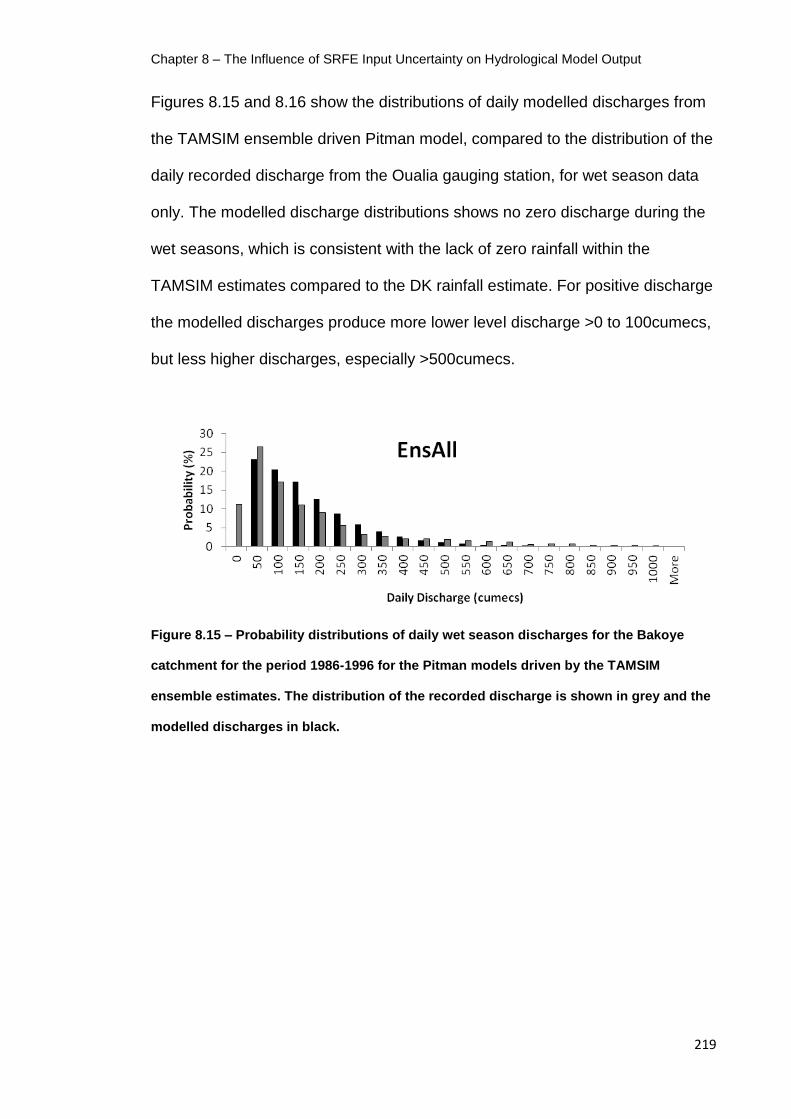
Chapter 8 – The Influence of SRFE Input Uncertainty on Hydrological Model Output
219
Figures 8.15 and 8.16 show the distributions of daily modelled discharges from
the TAMSIM ensemble driven Pitman model, compared to the distribution of the
daily recorded discharge from the Oualia gauging station, for wet season data
only. The modelled discharge distributions shows no zero discharge during the
wet seasons, which is consistent with the lack of zero rainfall within the
TAMSIM estimates compared to the DK rainfall estimate. For positive discharge
the modelled discharges produce more lower level discharge >0 to 100cumecs,
but less higher discharges, especially >500cumecs.
Figure 8.15 – Probability distributions of daily wet season discharges for the Bakoye
catchment for the period 1986-1996 for the Pitman models driven by the TAMSIM
ensemble estimates. The distribution of the recorded discharge is shown in grey and the
modelled discharges in black.
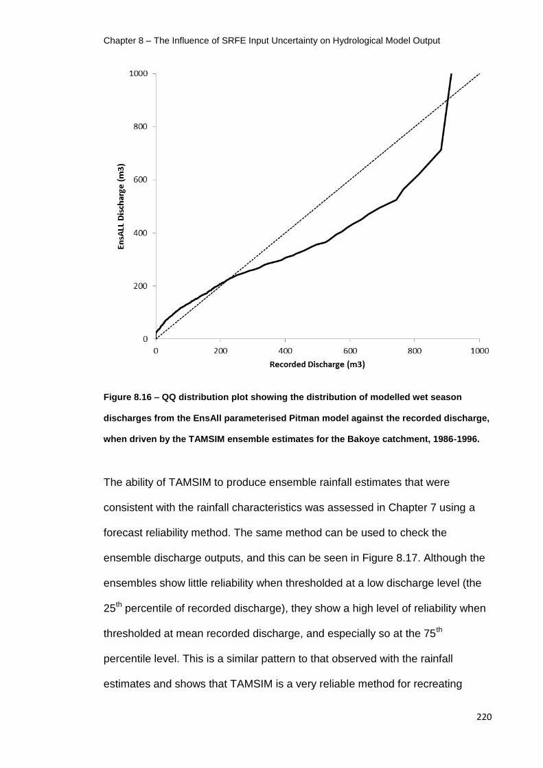
Chapter 8 – The Influence of SRFE Input Uncertainty on Hydrological Model Output
220
Figure 8.16 – QQ distribution plot showing the distribution of modelled wet season
discharges from the EnsAll parameterised Pitman model against the recorded discharge,
when driven by the TAMSIM ensemble estimates for the Bakoye catchment, 1986-1996.
The ability of TAMSIM to produce ensemble rainfall estimates that were
consistent with the rainfall characteristics was assessed in Chapter 7 using a
forecast reliability method. The same method can be used to check the
ensemble discharge outputs, and this can be seen in Figure 8.17. Although the
ensembles show little reliability when thresholded at a low discharge level (the
25th percentile of recorded discharge), they show a high level of reliability when
thresholded at mean recorded discharge, and especially so at the 75th
percentile level. This is a similar pattern to that observed with the rainfall
estimates and shows that TAMSIM is a very reliable method for recreating

Chapter 8 – The Influence of SRFE Input Uncertainty on Hydrological Model Output
221
rainfall characteristics for rainfall above trace level, and that this is passed on
through the Pitman model with some evidence that the reliability has been
strengthened further.
Figure 8.17 – Forecast reliability plots for daily wet season discharges for the Bakoye
Catchment for the period 1986-1996 for the Pitman model driven by the TAMSIM
ensemble estimates. The plot on the top-left shows values >23cumecs (the 25th
percentile
of the recorded discharge), the top-right shows values >202cumecs (the 75th
percentile of
the recorded discharge), and the bottom plot shows values >153cumecs (the mean daily
discharge of the recorded discharge). The dashed lines show the 1:1 relationship.
The final way to observe the performance of the TAMSIM ensemble estimate
driven Pitman model is to calculate performance statistics, for the entire 11 year

Chapter 8 – The Influence of SRFE Input Uncertainty on Hydrological Model Output
222
study period, and also for each individual wet season. The statistics can be
seen in Table 8.2.
RMSE (%) R2 BIAS (%)
1986-1996 89.08 0.52 0.80
1986 102.13 1.97 -52.73
1987 250.12 7.47 -177.86
1988 68.15 0.51 10.63
1989 105.58 1.14 -37.50
1990 108.17 2.26 -68.30
1991 73.65 0.61 2.44
1992 81.80 1.56 -32.09
1993 94.84 0.65 -9.80
1994 73.99 0.54 41.27
1995 70.20 0.53 32.43
1996 68.59 0.53 31.23
Table 8.2 – Performance statistics for the TAMSIM ensemble estimate driven Pitman
model for the whole 11 year study period, and for each individual wet season. RMSE and
BIAS are presented as a percentage of the mean daily discharge for each period.
The Influence of SRFE Bias on the Pitman Model
Chapter 7 demonstrated that TAMSIM was able to characterise the rainfall
characteristics for the daily Senegal rainfall field for the 11 year study period,
but it was also shown that the rainfall field displayed significant spatial and
temporal biases. The Pitman model has been used to model the hydrology in
the Bakoye catchment, an area that itself is affected by significant heterogeneity
in rainfall gradient. At its outlet the TAMSIM ensembles were shown to
underestimate the rainfall volumes compared to the underlying DK rain field,
and that this was a pattern seen in areas in the southern area of the Senegal
Basin, and the relationship changes with rainfall overestimated in the drier

Chapter 8 – The Influence of SRFE Input Uncertainty on Hydrological Model Output
223
north. The catchment average estimates for the TAMSIM ensemble rainfall
inputs were shown to be biased against the DK field, slightly underestimating
the rainfall in comparison – this can be attributed to the spatial biases in the
estimates. More significantly, the TAMSIM ensembles showed significant
interannual biases, with the method struggling to account for the large variations
of rainfall displayed by the catchment.
The EnsAll parameterisation of the Pitman model showed the least bias when
compared to the recorded discharge, with a BIAS of 0.8% of the mean daily
discharge. This suggests that the spatial bias in the TAMSIM SRFE is not
transferred to the Pitman model output as it pervades the entire rainfall input
and the SCE-UA calibration is able to compensate. The inability of TAMSIM to
estimate the interannual variations fully, however, has been observed
propagating through the model. Figures 8.18 to 8.20 show the relationship
between the TAMSIM estimate bias, the EnsAll model bias and the error in the
EnsAll model.

Chapter 8 – The Influence of SRFE Input Uncertainty on Hydrological Model Output
224
Figure 8.18 – Chart showing the relationship between the BIAS within the TAMSIM rainfall
estimates and the resulting BIAS from the EnsAll parameterised Pitman model – the BIAS
score is from all ensemble members.
Figure 8.19 – Chart showing the relationship between the BIAS within the TAMSIM rainfall
estimates and the mean RMSE from the EnsAll parameterised Pitman model – the BIAS
score is from all ensemble members.
-200
-150
-100
-50
0
50
100
-0.4 -0.2 0 0.2 0.4 0.6 0.8 1 1.2
Pit
man
BIA
S (c
um
ecs
)
TAMSIM BIAS (mm)

Chapter 8 – The Influence of SRFE Input Uncertainty on Hydrological Model Output
225
Figure 8.20 – Chart showing the relationship between the BIAS within the EnsAll
parameterised Pitman model and the mean RMSE from the same model – the BIAS score
is from all ensemble members.
It is clear from the charts shown in Figures 8.18 to 8.20 that the propagation of
the bias is not direct. Although the propagation of the bias does appear to be
roughly linear between TAMSIM and the EnsAll, it is not straightforward - an
unbiased TAMSIM rainfall estimate can be expected to result in a discharge
output with a BIAS of around -60cumecs. An unbiased discharge output is likely
to be produced by a TAMSIM estimate with a BIAS of 0.7mm. The best
performing models are driven by rainfall estimates showing a BIAS of 0.7mm.
The TAMSIM SRFE were shown in Chapter 7 to have a mean BIAS of 0.41mm
over the 11 year period, as overall TAMSIM underestimates rainfall in relation to
the DK rain field. This is overall BIAS influences the calibration of the Pitman
model, as it is calibrated against the biased estimate which explains why the
unbiased Pitman model exists when driven by a positively biased TAMSIM

Chapter 8 – The Influence of SRFE Input Uncertainty on Hydrological Model Output
226
estimate. This compensation for the overall underestimation of the rainfall by
TAMSIM results in an overestimation of the discharge even when the rainfall
estimate is lower than the DK estimate – for years when the TAMSIM
overestimates the rainfall, this bias is magnified by the Pitman model.
The charts shown in Figures 8.18 to 8.20 appear to be skewed by the data from
the 1987 wet season that displayed particularly poor correlation with the
recorded discharge. It is tempting to remove this year from the analysis but
there is no reason to assume that the data for that year is incorrect – it is likely
that it is limitations in the model processes that are the cause and it represents
an issue likely to be faced by such methods when applied to contemporary
data. In actuality, similar patterns remain visible even without the representation
of the 1987 data. It is not clear why the modelling of the 1987 wet season was
so poor, however the Bakoye average rainfall from the raingauges in 1987
showed a far greater deviation from the mean for the period than for the whole
catchment, and it is possible that this has been lost since the DK stage of the
process.
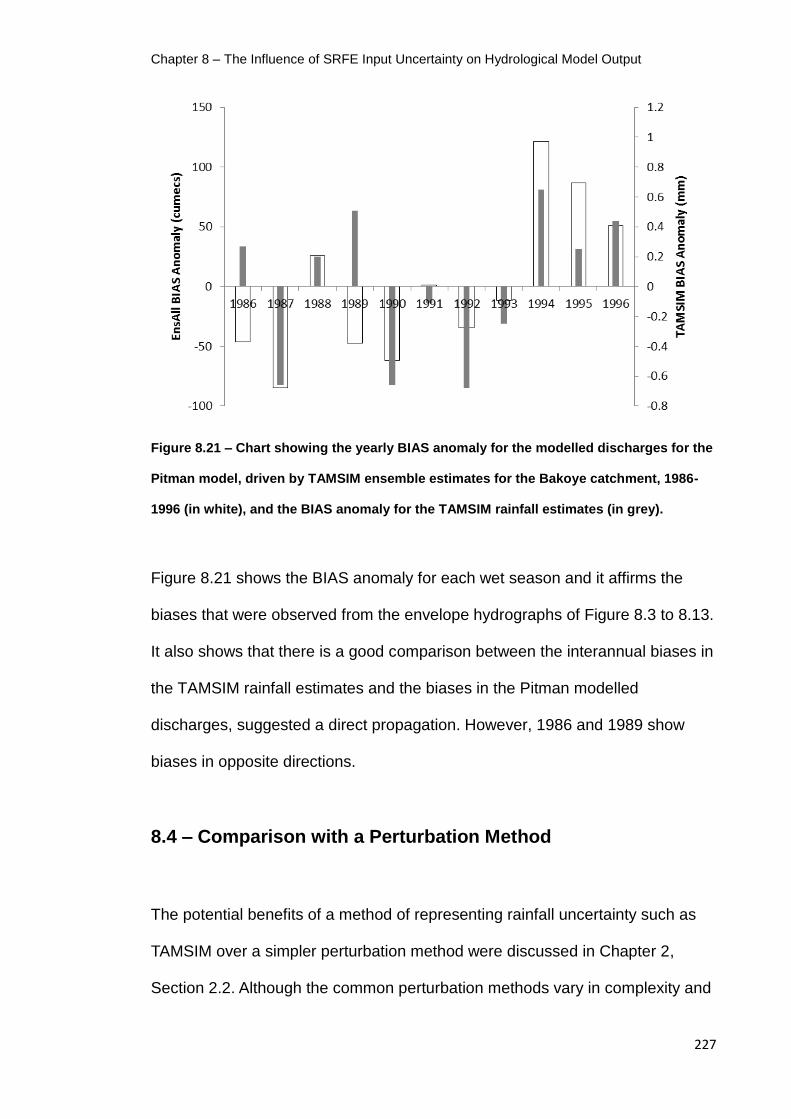
Chapter 8 – The Influence of SRFE Input Uncertainty on Hydrological Model Output
227
Figure 8.21 – Chart showing the yearly BIAS anomaly for the modelled discharges for the
Pitman model, driven by TAMSIM ensemble estimates for the Bakoye catchment, 1986-
1996 (in white), and the BIAS anomaly for the TAMSIM rainfall estimates (in grey).
Figure 8.21 shows the BIAS anomaly for each wet season and it affirms the
biases that were observed from the envelope hydrographs of Figure 8.3 to 8.13.
It also shows that there is a good comparison between the interannual biases in
the TAMSIM rainfall estimates and the biases in the Pitman modelled
discharges, suggested a direct propagation. However, 1986 and 1989 show
biases in opposite directions.
8.4 – Comparison with a Perturbation Method
The potential benefits of a method of representing rainfall uncertainty such as
TAMSIM over a simpler perturbation method were discussed in Chapter 2,
Section 2.2. Although the common perturbation methods vary in complexity and

Chapter 8 – The Influence of SRFE Input Uncertainty on Hydrological Model Output
228
direct relationship with the rainfall statistics, they generally only vary the amount
of rainfall in each timestep and do not account for occurrences when the rainfall
estimation fails to predict rainfall, or predicts rainfall when there was none. The
TAMSIM method is able to do this, as has been demonstrated in the section
above.
To demonstrate how a perturbation method will characterise rainfall uncertainty
differently from a full spatio-temporal distribution approach, the TAMSAT1 daily
rainfall values were randomly perturbed to produce a set of 200 ensemble
representations of rainfall. Although different ranges of values were tested, a
perturbation of up to 50% of the daily rainfall value produced an uncertainty
range of a similar magnitude to TAMSIM.
The hydrographs shown in Figures 8.22 to 8.31 compare the 95% confidence
discharge envelopes using the EnsAll parameterisation, when driven by the
TAMSIM ensemble SRFE inputs, and an ensemble input based on perturbing
the TAMSAT1 estimate by a randomly selected value from a uniform distribution
equal to 50% of the rainfall estimate (plus and minus).

Chapter 8 – The Influence of SRFE Input Uncertainty on Hydrological Model Output
229
Figure 8.22 – Hydrograph showing the 95% confidence discharge envelopes modelled by
the Pitman model for the Bakoye catchment in 1987, driven by TAMSIM ensemble SRFE
(shown in red) and an ensemble of up to 50% perturbed TAMSAT1 estimates (shown in
green).

Chapter 8 – The Influence of SRFE Input Uncertainty on Hydrological Model Output
230
Figure 8.23 – Hydrograph showing the 95% confidence discharge envelopes modelled by
the Pitman model for the Bakoye catchment in 1988, driven by TAMSIM ensemble SRFE
(shown in red) and an ensemble of up to 50% perturbed TAMSAT1 estimates (shown in
green).

Chapter 8 – The Influence of SRFE Input Uncertainty on Hydrological Model Output
231
Figure 8.24 – Hydrograph showing the 95% confidence discharge envelopes modelled by
the Pitman model for the Bakoye catchment in 1989, driven by TAMSIM ensemble SRFE
(shown in red) and an ensemble of up to 50% perturbed TAMSAT1 estimates (shown in
green).
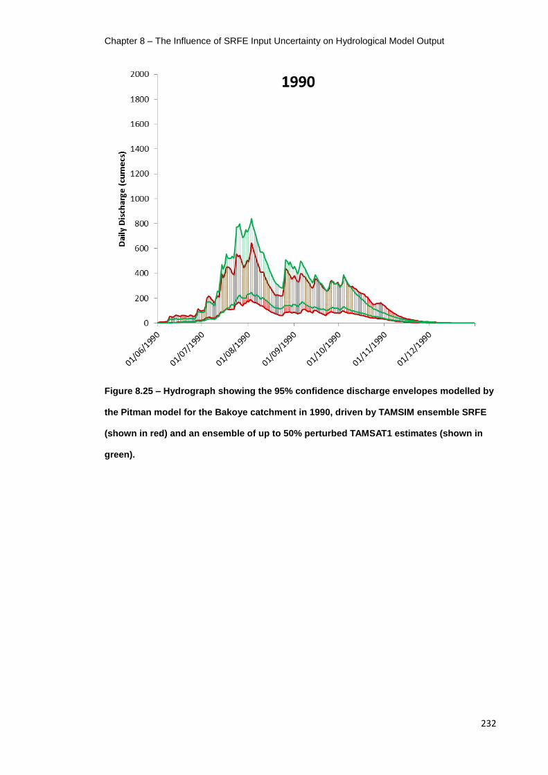
Chapter 8 – The Influence of SRFE Input Uncertainty on Hydrological Model Output
232
Figure 8.25 – Hydrograph showing the 95% confidence discharge envelopes modelled by
the Pitman model for the Bakoye catchment in 1990, driven by TAMSIM ensemble SRFE
(shown in red) and an ensemble of up to 50% perturbed TAMSAT1 estimates (shown in
green).

Chapter 8 – The Influence of SRFE Input Uncertainty on Hydrological Model Output
233
Figure 8.26 – Hydrograph showing the 95% confidence discharge envelopes modelled by
the Pitman model for the Bakoye catchment in 1991, driven by TAMSIM ensemble SRFE
(shown in red) and an ensemble of up to 50% perturbed TAMSAT1 estimates (shown in
green).

Chapter 8 – The Influence of SRFE Input Uncertainty on Hydrological Model Output
234
Figure 8.27 – Hydrograph showing the 95% confidence discharge envelopes modelled by
the Pitman model for the Bakoye catchment in 1992, driven by TAMSIM ensemble SRFE
(shown in red) and an ensemble of up to 50% perturbed TAMSAT1 estimates (shown in
green).

Chapter 8 – The Influence of SRFE Input Uncertainty on Hydrological Model Output
235
Figure 8.28 – Hydrograph showing the 95% confidence discharge envelopes modelled by
the Pitman model for the Bakoye catchment in 1993, driven by TAMSIM ensemble SRFE
(shown in red) and an ensemble of up to 50% perturbed TAMSAT1 estimates (shown in
green).
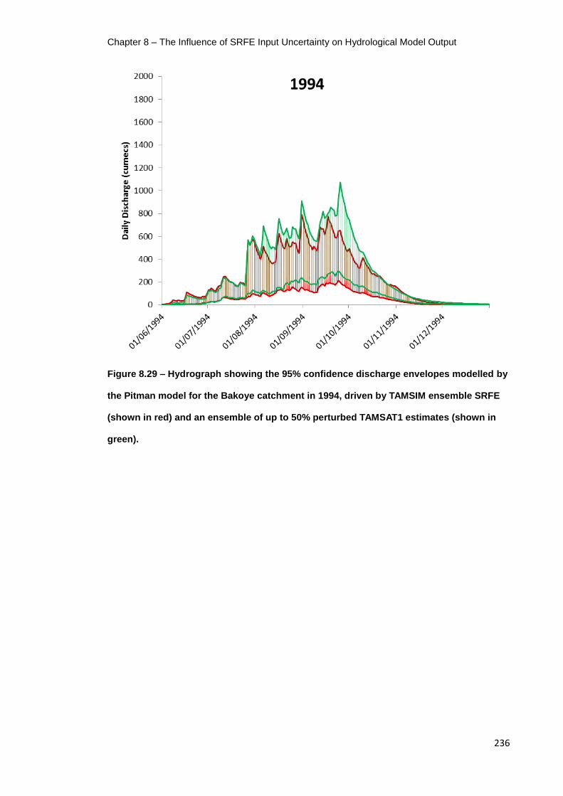
Chapter 8 – The Influence of SRFE Input Uncertainty on Hydrological Model Output
236
Figure 8.29 – Hydrograph showing the 95% confidence discharge envelopes modelled by
the Pitman model for the Bakoye catchment in 1994, driven by TAMSIM ensemble SRFE
(shown in red) and an ensemble of up to 50% perturbed TAMSAT1 estimates (shown in
green).

Chapter 8 – The Influence of SRFE Input Uncertainty on Hydrological Model Output
237
Figure 8.30 – Hydrograph showing the 95% confidence discharge envelopes modelled by
the Pitman model for the Bakoye catchment in 1995, driven by TAMSIM ensemble SRFE
(shown in red) and an ensemble of up to 50% perturbed TAMSAT1 estimates (shown in
green).

Chapter 8 – The Influence of SRFE Input Uncertainty on Hydrological Model Output
238
Figure 8.31 – Hydrograph showing the 95% confidence discharge envelopes modelled by
the Pitman model for the Bakoye catchment in 1996, driven by TAMSIM ensemble SRFE
(shown in red) and an ensemble of up to 50% perturbed TAMSAT1 estimates (shown in
green).
Although the perturbation method adopted for this test was a non-sophisticated
method and was not based on any measured statistics of uncertainty, the
hydrographs in Figures 8.22 to 8.31 do demonstrate the predicted principle that
a perturbation method is not fully characterising the uncertainty within the
TAMSAT1 rainfall estimate.
By comparing the two envelopes in each hydrograph, TAMSIM shows that the
uncertainty bounds within the TAMSAT1 SRFE are not symmetrical. This is an

Chapter 8 – The Influence of SRFE Input Uncertainty on Hydrological Model Output
239
assumption of the 50% perturbation method, which displays an envelope that
often exceeds the maximum values predicted by TAMSIM, yet does not predict
the lowest flows, especially for the months of August and September.
Section 8.2 demonstrated how TAMSIM was able to account for the temporal
non-stationarity of the relationship between CCD and rainfall, which was
particularly evident in the 95% confidence discharge envelopes after October of
each year. The perturbation method is dependent on the TAMSAT1
deterministic estimate, so makes the assumption that as the rainfall rate
decreases, so does the uncertainty – which is propagated into the discharge
output uncertainty. This is not the reality, as it has been seen that estimates
become relatively more uncertain and unreliable for lower discharges. TAMSIM
produces ensemble estimates that are independent of the TAMSAT1
deterministic estimate, and for the period after October for each year the
uncertainty envelopes are wider, and from Figures 8.3 to 8.13 there were even
some signs that the envelope and the deterministic estimate were becoming
decoupled.
8.5 – Conclusions
The Pitman model was calibrated using several estimates of rainfall and each
parameterisation was tested for use with the TAMSIM ensemble estimates. The
EnsTAM1 and EnsMean parameterisations showed particularly poor
transferablility with use with ensemble inputs, but a calibration that incorporated
each ensemble member in turn, EnsAll, showed the best performance of all the

Chapter 8 – The Influence of SRFE Input Uncertainty on Hydrological Model Output
240
parameterisations, with little bias evident over the entire 11 year period when
driven by the TAMSIM estimates. The EnsAll parameterisation was used to
model the ensemble discharge output from the Pitman model, and the output
used to produce the 95% confidence discharge envelopes for each year of the
record.
The influence of the input uncertainty on the Pitman model can be seen to be
great, with wide 95% confidence discharge envelopes visible in the hydrographs
of Figures 8.3 to 8.13, and 40.3% of days in the wet season seeing the
recorded discharge falling outside of these uncertainty bounds , and even with
consideration of up to 25% of observation error in the discharge data this was
only reduced to 28.8% - although the impact of this error propagating into model
parameter has not been considered and could be significant. This is not
unexpected as the data available for the calibration of TAMSAT1 was extremely
limited, and therefore the SRFE produced contained wide uncertainties, for all
three forms – spatial, temporal and rate. The cause of the mismatch between
the 95% confidence discharge envelopes and the recorded discharge is likely to
be bias resulting from anomalous years of rainfall, which, as a result of the large
interannual variations of rainfall in the regions, is almost every year. From
Figure 3.17 it can be seen that for the Bakoye catchment only three of the 11
years in the study displayed rainfall near the mean value for the period.
The bias within the TAMSIM SRFE is propagated directly to the Pitman model,
although due to interactions with the automatic calibration approach, the EnsAll
parameterised Pitman model favoured SRFE that display a positive bias. This

Chapter 8 – The Influence of SRFE Input Uncertainty on Hydrological Model Output
241
further erodes the performance of the Pitman model for years that display less
rainfall than the mean for the period.
The results for 1987 also show that local variations of the rainfall, relative the
catchment as a whole, have been lost. In 1987 the raingauges associated with
the Bakoye catchment showed that the area displayed lower rainfall than the
entire Senegal Basin, and this has been lost by assumptions of heterogeneity
inherent in the process – resulting in the poor representation of the 1987 wet
season discharges.
The TAMSIM algorithm has been shown to produce a more complete portrayal
of the uncertainty than a basic perturbation method. As TAMSIM is able to
account for all forms of uncertainty within the TAMSAT1 SRFE rather than just
an adjustment of the rate of rainfall, it is able to fully account for the uncertainty
caused by the non-stationary nature of the calibration, importantly in a way that
was independent to the TAMSAT1 SRFE itself. This becomes most evident for
the late wet season period from October each year, where the envelope
produced by the perturbation method narrows significantly when compared to
the TAMSIM modelled envelope. In addition the TAMSIM envelope shows signs
of independence from the TAMSAT1 deterministic estimate, which the
perturbation method does not as its envelope is symmetrical around TAMSAT1,
and the magnitude of uncertainty is dependent on the rain rate.
It is anticipated that when the presented methodology is repeated for a
catchment with greater data resources, where monthly climatic calibrations can

Chapter 8 – The Influence of SRFE Input Uncertainty on Hydrological Model Output
242
be calculated for TAMSAT1 and TAMSIM, the influence of the above effect will
become less visible. The non-stationarity of the calibration will logically be less
within a single month than over a highly variable 5 month wet season, however,
it is still a cause of uncertainty and had this test been performed on such a
catchment then this benefit of TAMSIM may have been missed.
It is suggested that when accounting for the influence of SRFE input uncertainty
on downstream models that the use of perturbation methods are inadequate,
and this has been demonstrated in this chapter. Only a fully spatially and
temporally distributed method, that uses a full conditional distribution in respects
to the input data, and not the deterministic estimate itself, to account for input
uncertainty is appropriate. This thesis has only investigated the influence of the
TAMSIM ensemble SRFE on a lumped CRR model, and there remains a
pressing research need for an investigation into the influence of full SRFE
uncertainty characterisation on distributed models – this is likely to be more
complex than for a lumped model structure.
The EnsAll method of parameterisation has been introduced in this chapter and
was shown to outperform all the alternative methods for calibrating the Pitman
model for use with ensemble inputs. However, the method still requires
validation against an independent dataset – this can be done using the 1997-
2005 discharge data from the Oualia gauging station, using TAMSIM SRFE
produced for the period using the 1986-1996 calibrations. This would be the
next logical step for expanding this research.
Chapter 9 – The Influence of Ensemble Rainfall Input on the Calibration of the Pitman Model
243
9 The Influence of Ensemble Rainfall
Input on the Calibration of the
Pitman Model
9.1 – Introduction
The previous chapter demonstrated how the uncertainty associated with the
TAMSAT1 SRFE propagated through the Pitman lumped CRR model, using
ensemble input and output datasets, and plotting 95% discharge confidence
envelopes, using the EnsAll parameterisation which was shown to be the
optimal calibration for use with the TAMSIM ensemble estimates. This chapter
further investigates the influence of the uncertainty on the calibration of the
Pitman model, with a particular focus on the model behaviour and the
relationship between model performance, behaviour and the parameters
selected.
Section 9.2 observes the model behaviour under different calibrations and
different rainfall inputs. Section 9.3 takes a closer look at the EnsInd parameter
sets, observing the relationships between the parameter values selected and
the model behaviour and performance. Section 9.4 concludes the chapter.

Chapter 9 – The Influence of Ensemble Rainfall Input on the Calibration of the Pitman Model
244
9.2 – Pitman Model Behaviours
This section looks at the various calibrations of the Pitman model, observing
their relative performance, and how the different inputs impact on the
performance and behaviour of the model. It will compare the performance of the
Pitman model using the four deterministic rainfall records, calibrated for the
1986-1996 study period.
RMSE as % of mean daily discharge
Gauge Average DK TAMSAT1 EnsMean
1987-1996 128.03 108.32 112.49 106.79
Table 9.1 – Table showing the 11 year calibration for the four rainfall inputs for the period
1987-1996.
The RMSE as % of mean daily discharges are shown in Table 9.1 for the period
of 1987 to 1996. The recorded and modelled discharges for 1986 were included
as part of the calibration but excluded from calculation of the errors, as the
modelled discharges from 1986 will be influenced by the initial conditions of the
Pitman model – although this was observed to be negligible in Chapter 8. The
best performing Pitman model was driven and calibrated using the daily mean
of the TAMSIM ensemble members, the EnsMean input, but the performance of
the DK driven and calibrated Pitman model showed comparable performance.
The TAMSAT1 driven and calibrated Pitman model outperformed the Gauge
Average driven and calibrated Pitman model, suggested that the additional
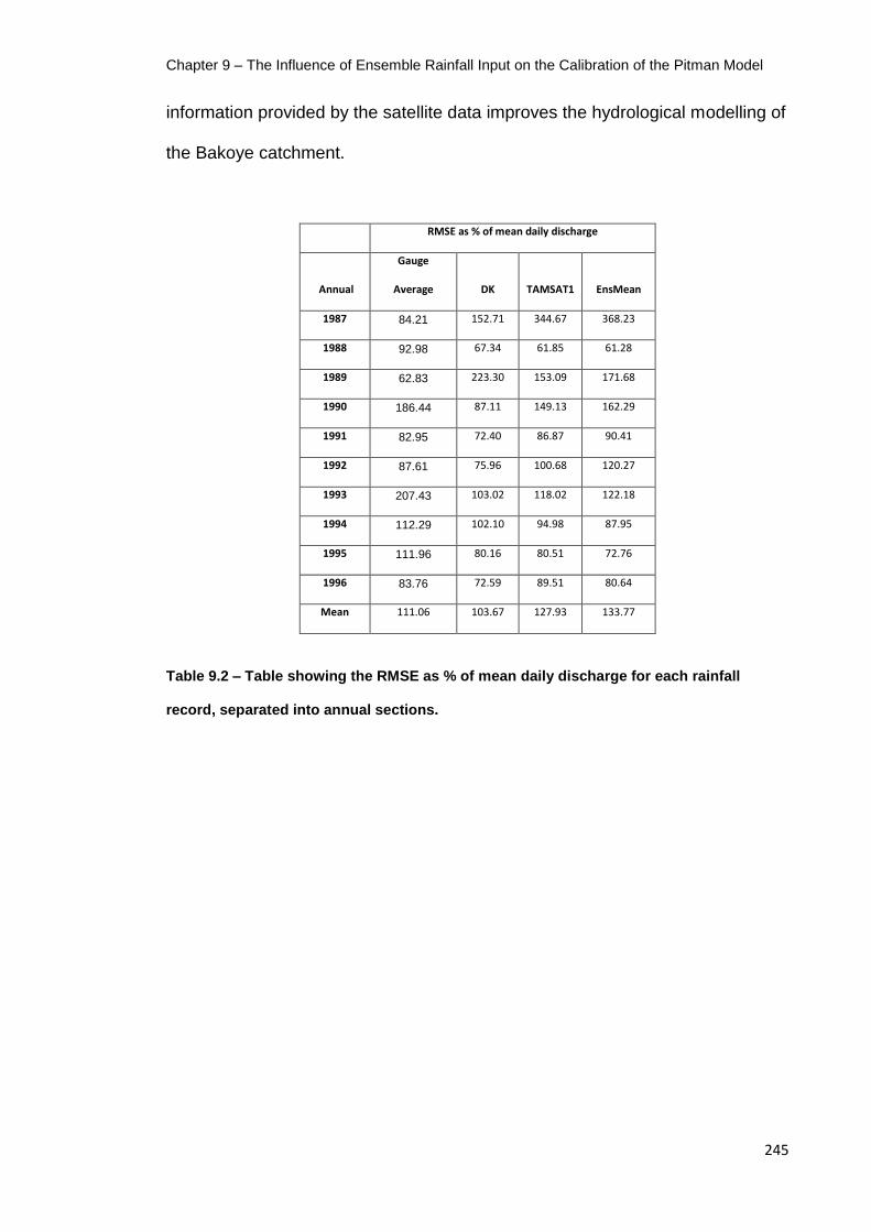
Chapter 9 – The Influence of Ensemble Rainfall Input on the Calibration of the Pitman Model
245
information provided by the satellite data improves the hydrological modelling of
the Bakoye catchment.
RMSE as % of mean daily discharge
Annual
Gauge
Average DK TAMSAT1 EnsMean
1987 84.21 152.71 344.67 368.23
1988 92.98 67.34 61.85 61.28
1989 62.83 223.30 153.09 171.68
1990 186.44 87.11 149.13 162.29
1991 82.95 72.40 86.87 90.41
1992 87.61 75.96 100.68 120.27
1993 207.43 103.02 118.02 122.18
1994 112.29 102.10 94.98 87.95
1995 111.96 80.16 80.51 72.76
1996 83.76 72.59 89.51 80.64
Mean 111.06 103.67 127.93 133.77
Table 9.2 – Table showing the RMSE as % of mean daily discharge for each rainfall
record, separated into annual sections.

Chapter 9 – The Influence of Ensemble Rainfall Input on the Calibration of the Pitman Model
246
RMSE as % of mean daily discharge
Wet Season
Gauge
Average DK TAMSAT1 EnsMean
1987 55.49 101.42 227.50 242.89
1988 61.80 44.30 40.58 40.29
1989 41.31 148.08 101.4862 113.82
1990 123.63 57.37 97.93 106.54
1991 58.76 48.48 58.26 60.64
1992 72.57 50.50 67.07 80.14
1993 136.79 67.93 77.78 80.49
1994 76.46 69.52 64.48 59.71
1995 75.54 54.08 54.39 49.13
1996 56.47 48.92 60.28 54.29
Mean 73.95 69.06 84.98 88.79
Table 9.3 – Table showing RMSE as % of mean daily discharge for each rainfall record,
separated into wet season sections.
Tables 9.2 and 9.3 show the error for each input when the discharge records
are split into annual and wet season sections. The DK rainfall input shows the
best performance at wet season scale, as well as annually. TAMSAT1 and
EnsMean show comparable performance at both scales but are out-performed
by Gauge Average estimate. The SRFE driven models, although showing
superior skill over the entire period, actually show inferior performance
compared to the Gauge Average estimate driven models when considered at
annual, or wet season periods. It is likely this is because of the systematic
biases in the SRFE caused by anomalous years of rainfall, meaning the SRFE
perform well compared to a long term mean but do not have sufficient flexibility
to account for shorter term variations.

Chapter 9 – The Influence of Ensemble Rainfall Input on the Calibration of the Pitman Model
247
Model Behaviour and Performance
Table 9.4 shows the proportion of modelled discharge originating from ground
water from the Pitman model when calibrated and driven using different
deterministic estimates, for 1986-1996.
Proportion of Modelled Discharge originating from Ground Water
(%)
Gauge
Average DK TAMSAT1 EnsMean
1986-1996 0.00 0.00 2.54 0.81
Table 9.4 – Proportions of modelled discharge originating from ground water as
modelled by the Pitman model, calibrated for different rainfall inputs for the period 1986-
1996.
For the period 1986-1996, when calibrated against deterministic estimates of
rainfall, the Pitman model does not model a significant proportion of ground
water flows, essentially operating as a single-bucket model (Table 9.4).

Chapter 9 – The Influence of Ensemble Rainfall Input on the Calibration of the Pitman Model
248
Figure 9.1 – Chart showing the proportion of EnsInd outputs against the proportion of
modelled discharge originating from ground water displayed by each model.
Figure 9.2 - Relationship between model performance as represented by RMSE as
percentage of mean daily actual discharge, and model behaviour as represented by
proportion of modelled discharge originating from ground water, for the EnsInd
parameterisations.

Chapter 9 – The Influence of Ensemble Rainfall Input on the Calibration of the Pitman Model
249
Figure 9.1 shows the spread of model behaviours displayed by the EnsInd
Pitman models, and Figure 9.2 shows the relationship between the model
behaviour and model performance for the EnsInd Pitman models. Although a
significant proportion of the models show zero ground water flow, or ground
water flows as <0.5% of the overall discharge, there is a distribution amongst
the remaining models, peaking at around 3.5% of the overall discharge.
There is a suggested relationship between model behaviour and performance,
as shown in Figure 9.2, where models that allow for some ground water flow
tend to display a better performance than those that allow for none, and that
when expressed as a simple linear relationship model performance increases
as the proportion of ground water increases.
When observing the model behaviour for the ensemble driven Pitman models
under different calibration regimes, it is clear that ground water flows again only
play a marginal role in determining the final modelled discharge. The EnsTAM1
outputs show a mean of 1.7% ground water flows from the TAMSIM ensemble
estimates, and the EnsAll outputs result in <0.005% ground water flows for
each ensemble. The EnsMean outputs, which were the most erratic and worst
performing, showed ground water flows up to 5%, but over 75% were <2.5%.

Chapter 9 – The Influence of Ensemble Rainfall Input on the Calibration of the Pitman Model
250
9.3 – Variability of Parameter Values for an Ensemble Driven
Pitman Model
This section investigates closely the individual parameter values for each
calibration and how these relate to the model behaviour and performance,
highlighting those parameters that are the most influential. The values for each
adjustable parameter, as described in Chapter 6, are observed in turn, showing
the distribution of calibrated values within the available parameter space.
The operation of the Pitman lumped CRR model has been described in Chapter
6, detailing each of the adjustable parameters and their purpose within the
model. For convenience the basic functionality of each parameter will be
described here also.
Zmin
The Zmin parameter is the minimum infiltration rate from the interception store to
the soil moisture store.

Chapter 9 – The Influence of Ensemble Rainfall Input on the Calibration of the Pitman Model
251
Figure 9.3 – Plot showing the box-whisker distribution of Zmin parameter values chosen
by automatic calibration of the TAMSIM ensemble members within the available
parameter space, for the Pitman lumped CRR model of the Bakoye Catchment between
1986 and 1996. The dot marks the mean value from the ensembles. Values selected by
automatic calibration against the deterministic rainfall estimates are shown for
comparison.

Chapter 9 – The Influence of Ensemble Rainfall Input on the Calibration of the Pitman Model
252
Figure 9.4 – Plot showing the relationship between the Zmin parameter values and the
proportion of modelled discharge from ground water, for the Pitman lumped CRR model
of the Bakoye Catchment for the period between 1986 and 1996, calibrated to individual
TAMSIM ensemble members.
Figure 9.5 – Plot showing the relationship between the Zmin parameter values and model
performance, for the Pitman lumped CRR model of the Bakoye Catchment for the period
between 1986 and 1996, calibrated to individual TAMSIM ensemble members.

Chapter 9 – The Influence of Ensemble Rainfall Input on the Calibration of the Pitman Model
253
The variation of the Zmin parameter between the EnsInd calibrations is minimal,
with most values <0.1mm.day-1, which is also evident for the other calibrated
values. The variation of Zmin values does not appear to influence the proportion
of modelled discharge from ground water, and does not appear to influence the
model performance. As the values do not vary greatly, this suggests that Zmin is
an important parameter determining model performance.
Zmax
The Zmax parameter controls the maximum rate of infiltration from the
interception store to the soil moisture store.
The Zmax parameter varies between 10 and 30mm.day-1 within the EnsInd
outputs, and these values are similar to the other calibrated values. There
appears to be a relationship between higher values of Zmax and a greater
proportion of modelled discharge originating from ground water, as seen in
Figure 9.7 – this is likely because the soil moisture store is being filled quicker
and more water is available to pass to the ground water store.
Figure 9.8 shows that the variation of the Zmax parameter value does not appear
to influence model performance, and the cluster of calibrations between 23 and
25mm.day-1 suggest that Zmax is influential to model performance.
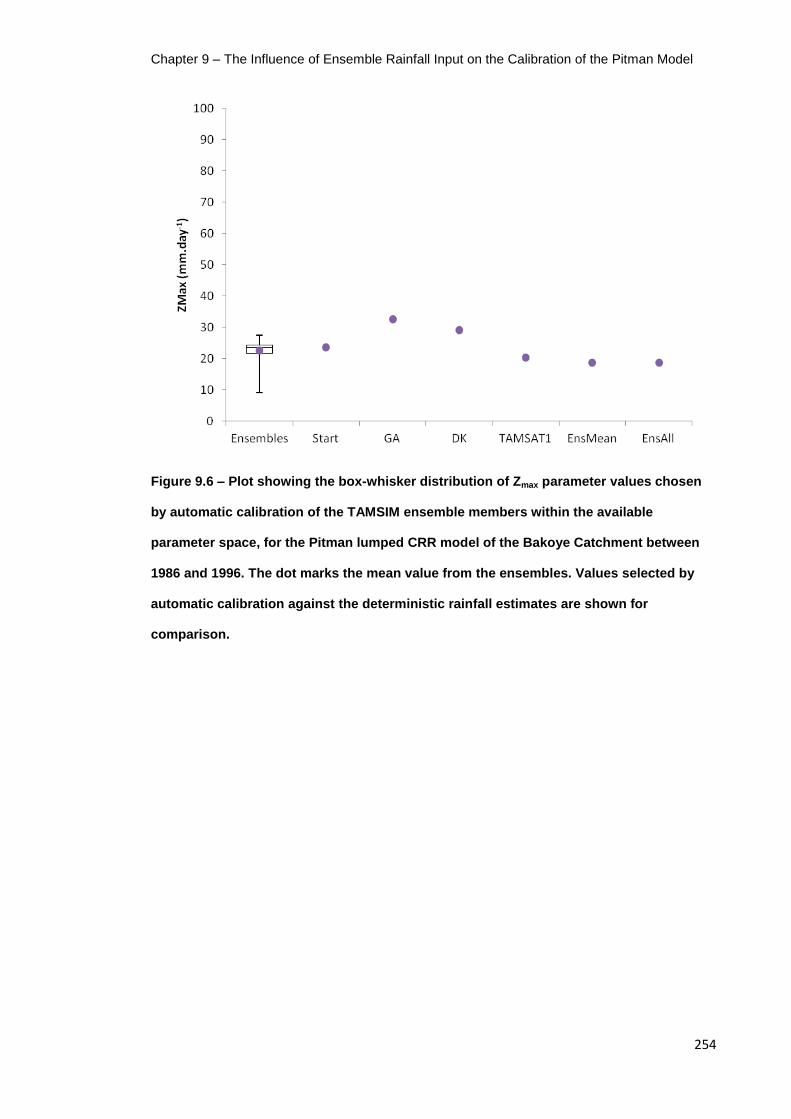
Chapter 9 – The Influence of Ensemble Rainfall Input on the Calibration of the Pitman Model
254
Figure 9.6 – Plot showing the box-whisker distribution of Zmax parameter values chosen
by automatic calibration of the TAMSIM ensemble members within the available
parameter space, for the Pitman lumped CRR model of the Bakoye Catchment between
1986 and 1996. The dot marks the mean value from the ensembles. Values selected by
automatic calibration against the deterministic rainfall estimates are shown for
comparison.
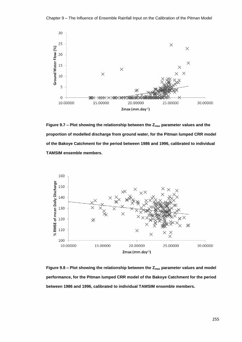
Chapter 9 – The Influence of Ensemble Rainfall Input on the Calibration of the Pitman Model
255
Figure 9.7 – Plot showing the relationship between the Zmax parameter values and the
proportion of modelled discharge from ground water, for the Pitman lumped CRR model
of the Bakoye Catchment for the period between 1986 and 1996, calibrated to individual
TAMSIM ensemble members.
Figure 9.8 – Plot showing the relationship between the Zmax parameter values and model
performance, for the Pitman lumped CRR model of the Bakoye Catchment for the period
between 1986 and 1996, calibrated to individual TAMSIM ensemble members.
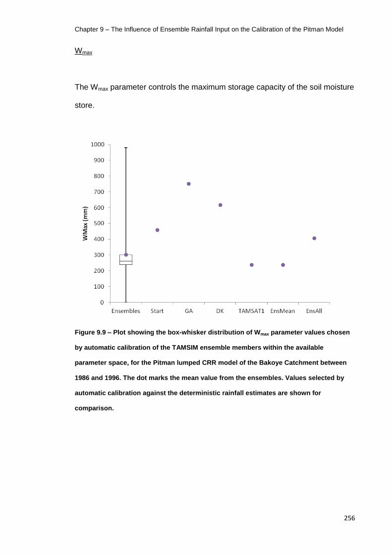
Chapter 9 – The Influence of Ensemble Rainfall Input on the Calibration of the Pitman Model
256
Wmax
The Wmax parameter controls the maximum storage capacity of the soil moisture
store.
Figure 9.9 – Plot showing the box-whisker distribution of Wmax parameter values chosen
by automatic calibration of the TAMSIM ensemble members within the available
parameter space, for the Pitman lumped CRR model of the Bakoye Catchment between
1986 and 1996. The dot marks the mean value from the ensembles. Values selected by
automatic calibration against the deterministic rainfall estimates are shown for
comparison.

Chapter 9 – The Influence of Ensemble Rainfall Input on the Calibration of the Pitman Model
257
Figure 9.10 – Plot showing the relationship between the Wmax parameter values and the
proportion of modelled discharge from ground water, for the Pitman lumped CRR model
of the Bakoye Catchment for the period between 1986 and 1996, calibrated to individual
TAMSIM ensemble members.
Figure 9.11 – Plot showing the relationship between the Wmax parameter values and
model performance, for the Pitman lumped CRR model of the Bakoye Catchment for the
period between 1986 and 1996, calibrated to individual TAMSIM ensemble members.

Chapter 9 – The Influence of Ensemble Rainfall Input on the Calibration of the Pitman Model
258
The Wmax parameter shows some variation throughout the whole of the
available parameter space, but a significant cluster of values between 200 and
300mm. Figure 9.10 shows that there is little relationship between the value of
Wmax and the proportion of ground water in the modelled discharge. Figure 9.11
shows that there is variation in model performance within the cluster of values
and that when the calibration has selected values beyond that, the model
performance ability decreases. The clustering of values implies that Wmax is
influential on the model performance.
Wmin
The Wmin parameter values controls the threshold that below which no water
can percolate from the soil moisture store to the ground water store, and as
such it would be reasonable to assume that the greater the Wmin value, the less
ground water will contribute to the final modelled discharge.

Chapter 9 – The Influence of Ensemble Rainfall Input on the Calibration of the Pitman Model
259
Figure 9.12 – Plot showing the box-whisker distribution of Wmin parameter values chosen
by automatic calibration of the TAMSIM ensemble members within the available
parameter space, for the Pitman lumped CRR model of the Bakoye Catchment between
1986 and 1996. The dot marks the mean value from the ensembles. Values selected by
automatic calibration against the deterministic rainfall estimates are shown for
comparison.

Chapter 9 – The Influence of Ensemble Rainfall Input on the Calibration of the Pitman Model
260
Figure 9.13 – Plot showing the relationship between the Wmin parameter values and the
proportion of modelled discharge from ground water, for the Pitman lumped CRR model
of the Bakoye Catchment for the period between 1986 and 1996, calibrated to individual
TAMSIM ensemble members.
Figure 9.14 – Plot showing the relationship between the Wmin parameter values and
model performance, for the Pitman lumped CRR model of the Bakoye Catchment for the
period between 1986 and 1996, calibrated to individual TAMSIM ensemble members.

Chapter 9 – The Influence of Ensemble Rainfall Input on the Calibration of the Pitman Model
261
There is a considerable amount of variation between the ensembles in regards
to the calibrated Wmin values, with the majority of values between 400 and
800mm (Figure 9.12). The mean value from the ensembles is over 600mm,
above the cluster of Wmax values, meaning the threshold for percolation is
beyond the maximum capacity of the store therefore restricting the model’s
ability to model ground water.
Figure 9.13 shows that the expected relationship between the proportion of
ground water flows and the value of Wmin does exist but is not very strong, likely
because of the restrictions above. The variation of Wmin values does not have a
relationship with model performance and as there is no significant clustering of
values it is likely that the value of Wmin is not influential on the final modelled
discharge.
Imax
The Imax parameter is the maximum capacity of the interception store and
therefore restricts the potential evapotranspiration from the model.
The Imax value shows almost no variation between the EnsInd calibrations and
the values from other calibrations, with the model preferring to minimise the
value as small as possible – the majority of values are <0.1mm (Figure 9.15).
This restricts the amount of rainfall immediately lost by evapotranspiration.

Chapter 9 – The Influence of Ensemble Rainfall Input on the Calibration of the Pitman Model
262
The lack of variation means that there is little relationship between the varying
values and model behaviour and performance, but does suggest that Imax is
influential to the model performance.
Figure 9.15 – Plot showing the box-whisker distribution of Imax parameter values chosen
by automatic calibration of the TAMSIM ensemble members within the available
parameter space, for the Pitman lumped CRR model of the Bakoye Catchment between
1986 and 1996. The dot marks the mean value from the ensembles. Values selected by
automatic calibration against the deterministic rainfall estimates are shown for
comparison.

Chapter 9 – The Influence of Ensemble Rainfall Input on the Calibration of the Pitman Model
263
Figure 9.16 – Plot showing the relationship between the Imax parameter values and the
proportion of modelled discharge from ground water, for the Pitman lumped CRR model
of the Bakoye Catchment for the period between 1986 and 1996, calibrated to individual
TAMSIM ensemble members.
Figure 9.17 – Plot showing the relationship between the Imax parameter values and model
performance, for the Pitman lumped CRR model of the Bakoye Catchment for the period
between 1986 and 1996, calibrated to individual TAMSIM ensemble members.
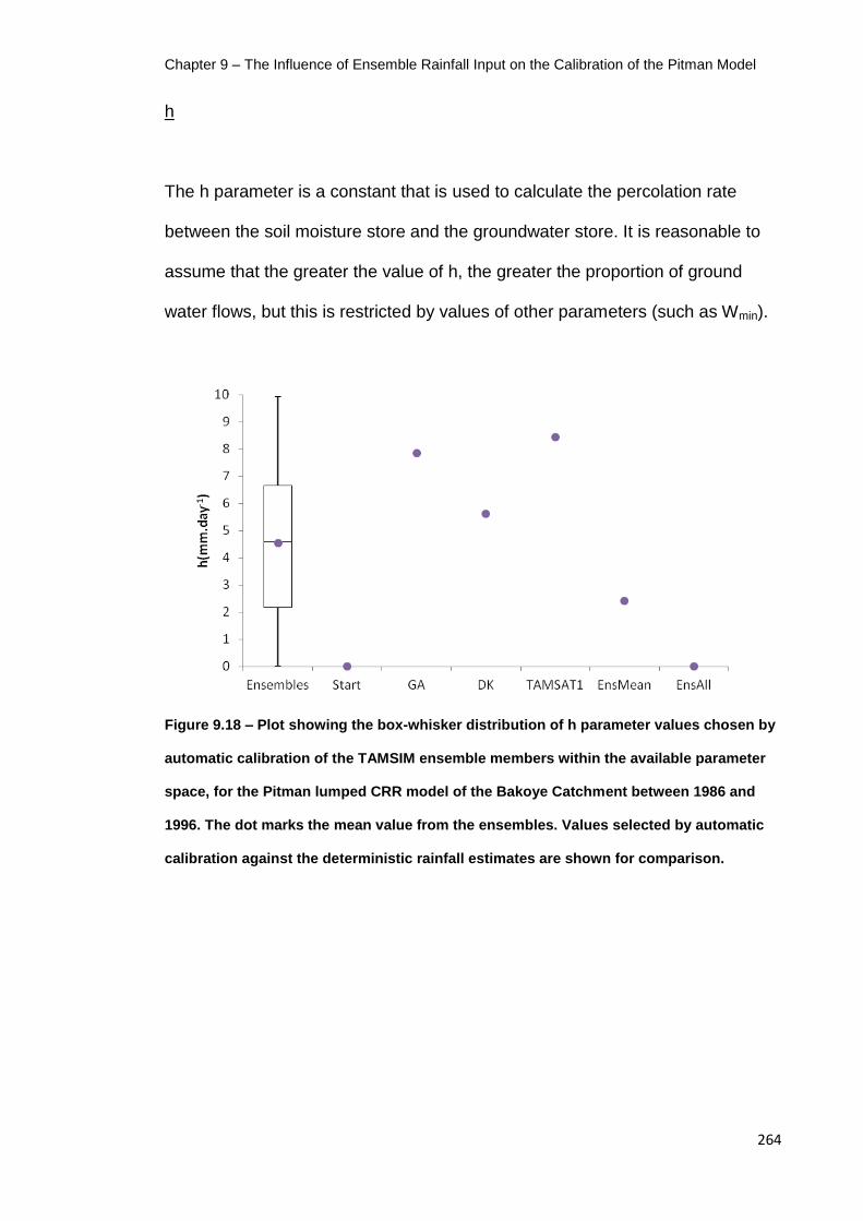
Chapter 9 – The Influence of Ensemble Rainfall Input on the Calibration of the Pitman Model
264
h
The h parameter is a constant that is used to calculate the percolation rate
between the soil moisture store and the groundwater store. It is reasonable to
assume that the greater the value of h, the greater the proportion of ground
water flows, but this is restricted by values of other parameters (such as Wmin).
Figure 9.18 – Plot showing the box-whisker distribution of h parameter values chosen by
automatic calibration of the TAMSIM ensemble members within the available parameter
space, for the Pitman lumped CRR model of the Bakoye Catchment between 1986 and
1996. The dot marks the mean value from the ensembles. Values selected by automatic
calibration against the deterministic rainfall estimates are shown for comparison.

Chapter 9 – The Influence of Ensemble Rainfall Input on the Calibration of the Pitman Model
265
Figure 9.19 – Plot showing the relationship between the h parameter values and the
proportion of modelled discharge from ground water, for the Pitman lumped CRR model
of the Bakoye Catchment for the period between 1986 and 1996, calibrated to individual
TAMSIM ensemble members.
Figure 9.20 – Plot showing the relationship between the h parameter values and model
performance, for the Pitman lumped CRR model of the Bakoye Catchment for the period
between 1986 and 1996, calibrated to individual TAMSIM ensemble members.

Chapter 9 – The Influence of Ensemble Rainfall Input on the Calibration of the Pitman Model
266
The values for h are reasonably equally distributed throughout the parameter
space available for the EnsInd calibrations, with a mean close to 5mm.day-1, in
the centre of the space (Figure 9.18). Surprisingly there is very little correlation
between the value of h and the proportion of the modelled discharge originating
from ground water (Figure 9.19), and a slight improvement of model
performance as h increases can be seen in Figure 9.20, although with no
significant clustering of values h is not influential on model performance, but this
is likely because of the high values of Wmin observed.
i
The i parameter value is used in conjunction with the h value to calculate the
percolation rate between the soil moisture store and the ground water store,
and therefore should be similarly related to model behaviour and performance.
As expected, i displays a similar pattern to h in regards to spread of values and
relationship between the values and model behaviour and performance, as
seen in Figures 9.21 to 9.23. The influence of i is restricted by the high Wmin
values that inhibit the periods where percolation can occur.
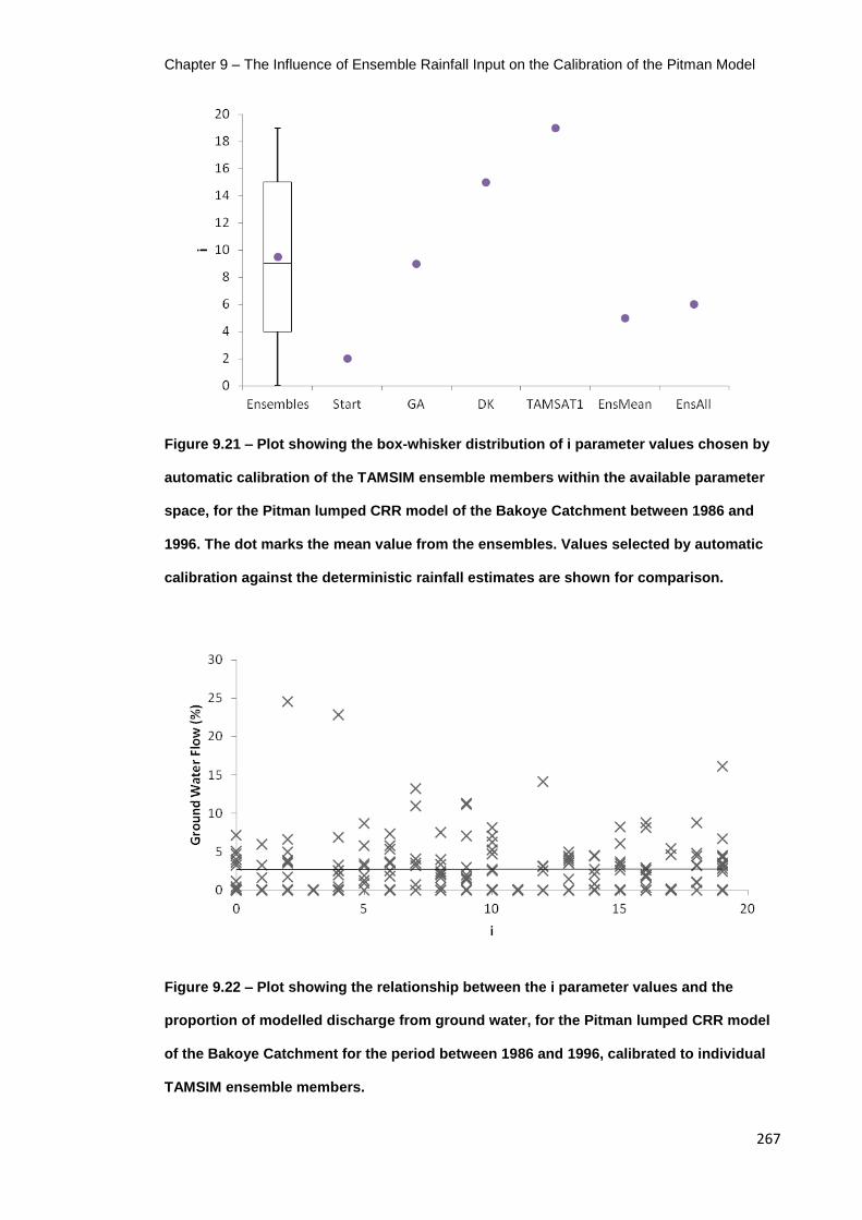
Chapter 9 – The Influence of Ensemble Rainfall Input on the Calibration of the Pitman Model
267
Figure 9.21 – Plot showing the box-whisker distribution of i parameter values chosen by
automatic calibration of the TAMSIM ensemble members within the available parameter
space, for the Pitman lumped CRR model of the Bakoye Catchment between 1986 and
1996. The dot marks the mean value from the ensembles. Values selected by automatic
calibration against the deterministic rainfall estimates are shown for comparison.
Figure 9.22 – Plot showing the relationship between the i parameter values and the
proportion of modelled discharge from ground water, for the Pitman lumped CRR model
of the Bakoye Catchment for the period between 1986 and 1996, calibrated to individual
TAMSIM ensemble members.
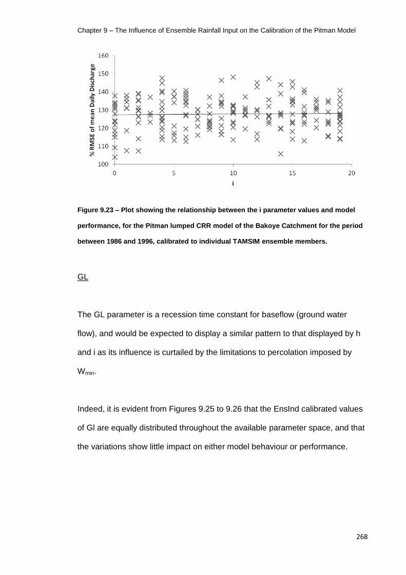
Chapter 9 – The Influence of Ensemble Rainfall Input on the Calibration of the Pitman Model
268
Figure 9.23 – Plot showing the relationship between the i parameter values and model
performance, for the Pitman lumped CRR model of the Bakoye Catchment for the period
between 1986 and 1996, calibrated to individual TAMSIM ensemble members.
GL
The GL parameter is a recession time constant for baseflow (ground water
flow), and would be expected to display a similar pattern to that displayed by h
and i as its influence is curtailed by the limitations to percolation imposed by
Wmin.
Indeed, it is evident from Figures 9.25 to 9.26 that the EnsInd calibrated values
of Gl are equally distributed throughout the available parameter space, and that
the variations show little impact on either model behaviour or performance.

Chapter 9 – The Influence of Ensemble Rainfall Input on the Calibration of the Pitman Model
269
Figure 9.24 – Plot showing the box-whisker distribution of GL parameter values chosen
by automatic calibration of the TAMSIM ensemble members within the available
parameter space, for the Pitman lumped CRR model of the Bakoye Catchment between
1986 and 1996. The dot marks the mean value from the ensembles. Values selected by
automatic calibration against the deterministic rainfall estimates are shown for
comparison.
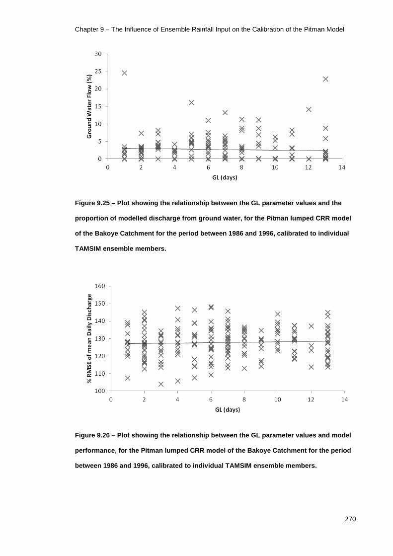
Chapter 9 – The Influence of Ensemble Rainfall Input on the Calibration of the Pitman Model
270
Figure 9.25 – Plot showing the relationship between the GL parameter values and the
proportion of modelled discharge from ground water, for the Pitman lumped CRR model
of the Bakoye Catchment for the period between 1986 and 1996, calibrated to individual
TAMSIM ensemble members.
Figure 9.26 – Plot showing the relationship between the GL parameter values and model
performance, for the Pitman lumped CRR model of the Bakoye Catchment for the period
between 1986 and 1996, calibrated to individual TAMSIM ensemble members.

Chapter 9 – The Influence of Ensemble Rainfall Input on the Calibration of the Pitman Model
271
TL
The TL parameter is a constant used in the calculation of the quick flow (surface
flow).
Figure 9.27 – Plot showing the box-whisker distribution of TL parameter values chosen
by automatic calibration of the TAMSIM ensemble members within the available
parameter space, for the Pitman lumped CRR model of the Bakoye Catchment between
1986 and 1996. The dot marks the mean value from the ensembles. Values selected by
automatic calibration against the deterministic rainfall estimates are shown for
comparison.

Chapter 9 – The Influence of Ensemble Rainfall Input on the Calibration of the Pitman Model
272
Figure 9.28 – Plot showing the relationship between the TL parameter values and the
proportion of modelled discharge from ground water, for the Pitman lumped CRR model
of the Bakoye Catchment for the period between 1986 and 1996, calibrated to individual
TAMSIM ensemble members.
Figure 9.29 – Plot showing the relationship between the TL parameter values and model
performance, for the Pitman lumped CRR model of the Bakoye Catchment for the period
between 1986 and 1996, calibrated to individual TAMSIM ensemble members.

Chapter 9 – The Influence of Ensemble Rainfall Input on the Calibration of the Pitman Model
273
The small variation of TL values from the EnsInd calibrations, similar to the
values from the other calibrations, suggests that the TL value is influential to the
model performance (Figure 9.27). The lack of variation results in little
relationship between the variation of values of TL and model behaviour and
performance (Figure 9.28 and 9.29).
Qq Lag
The Qq Lag parameter is a simple lag of the quick flow (surface flow) by
timesteps, in this case days.
Figure 9.30 – Plot showing the box-whisker distribution of Qq Lag parameter values
chosen by automatic calibration of the TAMSIM ensemble members within the available
parameter space, for the Pitman lumped CRR model of the Bakoye Catchment between
1986 and 1996. The dot marks the mean value from the ensembles. Values selected by
automatic calibration against the deterministic rainfall estimates are shown for
comparison.

Chapter 9 – The Influence of Ensemble Rainfall Input on the Calibration of the Pitman Model
274
Figure 9.31 – Plot showing the relationship between the Qq Lag parameter values and the
proportion of modelled discharge from ground water, for the Pitman lumped CRR model
of the Bakoye Catchment for the period between 1986 and 1996, calibrated to individual
TAMSIM ensemble members.
Figure 9.32 – Plot showing the relationship between the Qq Lag parameter values and
model performance, for the Pitman lumped CRR model of the Bakoye Catchment for the
period between 1986 and 1996, calibrated to individual TAMSIM ensemble members.

Chapter 9 – The Influence of Ensemble Rainfall Input on the Calibration of the Pitman Model
275
The majority of the EnsInd calibrations showed a Qq Lag of 1 day (Figure 9.30),
but there is some variation up to 2 days. Figure 9.31 shows that the higher Qq
Lag displays lower proportions of ground water flows, suggesting that the model
is attempting to compensate, probably at the end of the wet season. Figure 9.32
also suggests that there is a slight degradation in model performance as the
values increase.
Qb Lag
The Qb Lag parameter is a simple timestep (days) lag on the base flow (ground
water flow). Any influence of this parameter on model performance is dictated
largely by values of Wmin, h and i, which control the amount of rainfall reaching
the ground water store. As seen above, the Wmin values have constricted
percolation to the ground water store, so the influence of Qb Lag is likely to be
slight.
There is little to be seen in Figure 9.33 to 9.35 as regards to the possible
contribution of the Qb Lag on the performance of the Pitman lumped CRR
because of the restrictions from the high values of Wmin.

Chapter 9 – The Influence of Ensemble Rainfall Input on the Calibration of the Pitman Model
276
Figure 9.33 – Plot showing the box-whisker distribution of Qb Lag parameter values
chosen by automatic calibration of the TAMSIM ensemble members within the available
parameter space, for the Pitman lumped CRR model of the Bakoye Catchment between
1986 and 1996. The dot marks the mean value from the ensembles. Values selected by
automatic calibration against the deterministic rainfall estimates are shown for
comparison.
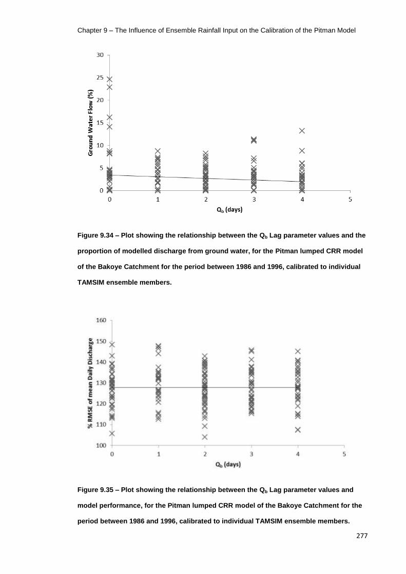
Chapter 9 – The Influence of Ensemble Rainfall Input on the Calibration of the Pitman Model
277
Figure 9.34 – Plot showing the relationship between the Qb Lag parameter values and the
proportion of modelled discharge from ground water, for the Pitman lumped CRR model
of the Bakoye Catchment for the period between 1986 and 1996, calibrated to individual
TAMSIM ensemble members.
Figure 9.35 – Plot showing the relationship between the Qb Lag parameter values and
model performance, for the Pitman lumped CRR model of the Bakoye Catchment for the
period between 1986 and 1996, calibrated to individual TAMSIM ensemble members.

Chapter 9 – The Influence of Ensemble Rainfall Input on the Calibration of the Pitman Model
278
9.4 – Conclusions
This chapter has investigated the influence of SRFE uncertainty on the
calibration, performance and behaviour of a hydrological model. The TAMSIM
algorithm has been used to produce 200 ensemble realisations of the daily
Senegal Basin rain field, each unique yet equiprobable within the bounds of
uncertainty when using the TAMSAT1 method for producing a SRFE. For each
ensemble member a rainfall input was produced and used to calibrate a Pitman
lumped CRR model of the Bakoye catchment for the period 1986 to 1996.
Using the proportion of modelled discharge originating from ground water as a
proxy for model behaviour, the majority of the Pitman calibrations resulted in
only a minor fraction of the total discharge as having originated from
groundwater flows. Of the deterministic Pitman models, the TAMSAT1 driven
and calibrated Pitman model showed the greatest proportion of ground water
flows but this was still only 2.52% of the total discharge.
For the EnsInd calibrations of the Pitman model to each of the 200 TAMSIM
ensemble inputs, the calibrations were also biased towards model behaviours of
very little or no ground water flows. The highest proportion of ground water in
modelled discharge was 25%, but the vast majority of the models showed <5%
and most 0%. Despite this, there is evidence that a greater proportion of ground
water modelled by the Pitman model does produce a better model performance
(Figure 9.2).

Chapter 9 – The Influence of Ensemble Rainfall Input on the Calibration of the Pitman Model
279
The relationship between model behaviour and model performance observed in
the EnsInd calibrations is contradictory, with the calibrations overwhelmingly
favouring a set of parameters that produce minimal or no ground water flows,
yet those that do show a greater proportion of ground water flows have a
tendency towards superior performance. Observation of the relationship
between model behaviour and parameter values suggests that the proportion of
ground water is largely dependent on the Wmin parameter, which controls the
minimum threshold of water stored in W, the soil moisture bucket, before
percolation can begin between the soil moisture store and the ground water
store. The calibration of Wmin is not dependent on the parameter selected for
Wmax, and both have the same parameter space available - in numerous cases
the Wmin threshold was greater than the Wmax maximum storage for the bucket,
resulting in the inability of water to transfer into the ground water store. This can
be seen as a flaw in the Pitman model and the calibration method selected, yet
the parameter spaces were wide and the calibration method was sufficiently
open for it to select parameter values that allowed for percolation and it
favoured not doing so. This could be tested fully by replacing the numerical
calibration of Wmin with a proportion of the Wmax value instead, and observing
whether the SCE-UA algorithm still opts for a restricted calibration – initial tests
have shown no improvement in model performance.
In terms of the impact of uncertainty within the SRFE on the calibration of the
Pitman model, this appears to be quite limited. The calibration of the
parameters that had the most influence on the model performance are
reasonably consistent throughout the EnsInd calibrations. This would indicate

Chapter 9 – The Influence of Ensemble Rainfall Input on the Calibration of the Pitman Model
280
that the majority of the spread of discharges seen in the hydrograph envelopes
of Chapter 8 has originated from variations in the input and not because of
variations between the hydrological models.
The model behaviours do suggest an element of equifinality that the SCE-UA
cannot reflect. The SCE-UA algorithm has been seen to be consistent in
selecting optimal sets of parameters, especially for those parameters that have
been shown to be influential for the performance of the model, but some
variability in the parameters show greater proportions of ground water flows with
increased model performance. This suggests that there are parameter sets
which allow greater proportions of ground water flow, with comparable
performance, that could be used for the Pitman model. A possible solution to
this would be to perform recalibration of the EnsInd models using a modified
Pitman, where the Wmin value is a proportion of Wmax, rather than a set value in
the parameter space – although initial tests have shown no improvement in
model performance, there may be differences in model behaviour.
Chapter 10 – Discussion
281
10 Discussion
10.1 – Key Results
The main aim of this thesis was to demonstrate how a fully spatio-temporally
distributed stochastic ensemble method could be used to characterise
uncertainty within a satellite rainfall estimate, and how the ensembles produced
could be used to drive and calibrate a deterministic hydrological model using
traditional hydrological methods. The thesis used the Senegal Basin as its study
area and daily rainfall estimates were produced using the TAMSAT1 method,
calibrated using a sparse raingauge network. The uncertainty within the
deterministic TAMSAT1 estimate was characterised using the TAMSIM method,
and 200 unique yet equiprobable rainfall estimates for the 1986-1996 study
period were produced.
It would be prudent here to highlight the benefits of using satellite data to
estimate rainfall for use as a driver for hydrological modelling. This thesis has
not used the full spatial distribution afforded by the method, which could be
achieved with the use of a distributed, or semi-distributed hydrological model,
however, the additional information provided by the SRFE can be seen to
improve the hydrological modelling of the Bakoye catchment when compared to

Chapter 10 – Discussion
282
an estimate from the raingauges. Table 9.1 shown in the previous chapter
showed the relative skill of each Pitman model, driven and calibrated by the
same input, showing that both the model using the TAMSAT1 estimate and the
mean of the TAMSIM ensembles displayed superior performance over the
Gauge Average estimate driven model. There was little evidence from observed
hydrographs that the use of the SRFE allowed for better prediction of peak
discharge timings, although Figure 10.1 shows an example which demonstrates
the potential of SRFE to improve discharge estimation.
The use of SRFE also provide additional information for areas or periods where
no gauge data is available. The use of historic raingauge data for the calibration
of the TAMSAT1, TAMSIM, and Pitman model methods allows for the
production of rainfall and discharge estimates for time periods outside this
calibration period, even if no ground recorded rainfall data is available.
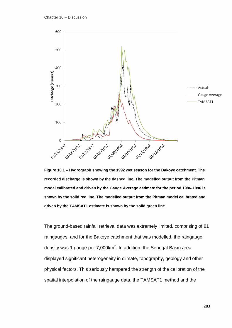
Chapter 10 – Discussion
283
Figure 10.1 – Hydrograph showing the 1992 wet season for the Bakoye catchment. The
recorded discharge is shown by the dashed line. The modelled output from the Pitman
model calibrated and driven by the Gauge Average estimate for the period 1986-1996 is
shown by the solid red line. The modelled output from the Pitman model calibrated and
driven by the TAMSAT1 estimate is shown by the solid green line.
The ground-based rainfall retrieval data was extremely limited, comprising of 81
raingauges, and for the Bakoye catchment that was modelled, the raingauge
density was 1 gauge per 7,000km2. In addition, the Senegal Basin area
displayed significant heterogeneity in climate, topography, geology and other
physical factors. This seriously hampered the strength of the calibration of the
spatial interpolation of the raingauge data, the TAMSAT1 method and the

Chapter 10 – Discussion
284
TAMSIM algorithm, resulting in a wet season climatic calibration having to be
adopted for each when a monthly calibration would have been preferred.
Teo (2006) found that because TAMSAT1 relied upon a climatic calibration
based on historic raingauge data it displayed significant bias in years of
anomalous rainfall – underestimating in years of heavy rainfall and
overestimating in drier years. This was also found to be the case for the
Senegal Basin, which was particularly marked due to the high degree of
interannual variation of rainfall for the region and within the study period. The
same was true for TAMSIM.
The TAMSIM ensembles were shown to be able to reproduce the spatial and
temporal distributions of rainfall, as well as the fractional nature of the rainfall as
displayed by the DK rain fields. However, the TAMSIM ensemble rain fields
were not able to reflect the significant rainfall gradient across the Senegal Basin
region, showing overestimation of rainfall in the drier north, and underestimation
in the wetter south. The full analysis of the performance of the TAMSIM
algorithm to reproduce the underlying DK rain field is shown in Chapter 7.
It was found that the Pitman model calibrated using the TAMSAT1 input was not
transferable for use with the TAMSIM ensemble inputs, neither was a calibration
against the daily mean of the TAMSIM ensembles. A calibration of the Pitman
model was performed using an input that incorporated all of the ensemble
members, essentially a 2,200 year record of rainfall and discharge data. This
proved to be computationally expensive but did produce a calibration for the

Chapter 10 – Discussion
285
Pitman model, that when driven by the ensemble members showed good
transferable performance and little overall bias.
The output from the TAMSIM ensemble driven Pitman model was used to
model the propagation of the input uncertainty through the Pitman model, and
95% confidence discharge envelopes were produced for each wet season in the
study period, showing the bounds of the uncertainty. The bounds showed that
the TAMSIM algorithm could not reflect the full uncertainty in the TAMSAT1
calibration, with the interannual variations in rainfall resulting in considerable
biases, with 40.3% of days in the wet seasons 1987-1996 showing the recorded
rainfall outside of the uncertainty bounds modelled.
However, TAMSIM displayed skill in representing uncertainty due to the non-
stationary nature of the calibration of TAMSAT1 over the wet season, with the
bounds better representing the recorded discharges for each year after the 1st
October, displaying independence from the deterministic estimate.
Despite the evident bias associated with interannual variations of rainfall, the
fully spatio-temporally distributed method of TAMSIM was shown to be superior
to the more established perturbation method. TAMSIM has the significant
advantage of modelling uncertainty independent of the deterministic estimate,
which the simple perturbation method could not, resulting in the reflection of
uncertainty bounds that were not symmetrical and occasionally decoupled
altogether as in the case above (Chapter 8).

Chapter 10 – Discussion
286
Finally, it was shown that the influence of the input uncertainty on the calibration
of the Pitman model was minimal. The review in Chapter 9 showed the
relationship between parameter values and model behaviour and performance
when the Pitman model was calibrated against the individual ensemble
members. For those parameters that were shown to be influential to the
performance there was little variation across the calibrations, indicating that an
optimal set of parameters, or a small distribution of parameter values, was
appropriate for use with all the ensemble members.
Model behaviour across the calibrations was fairly consistent with the majority
of the calibrated models preferring to limit the amount of discharge that
originated from ground water. It is not clear whether this was an issue with the
model structure, related to the way the Wmin value is determined in an automatic
calibration method, but the SCE-UA had sufficient freedom to model higher
proportions of groundwater if this improved performance. However, there was
significant variation in the performances to point to equifinality in the method,
with some models showing improved performance with greater proportions of
groundwater.
10.2 – Issues and Recommendations
The results from this thesis, as summarised above, demonstrate the ability of
the TAMSIM algorithm to fully characterise the uncertainty within a TAMSAT1
SRFE in a way that can be applied to a hydrological model to show the
propagation of that uncertainty. It has also demonstrated the principle that the
Chapter 10 – Discussion
287
full spatial and temporal characterisation of the uncertainty, within the bounds of
the underlying DK rain field, is superior to a simpler perturbation method.
Systematic Bias and Interannual Variations in Rainfall
The major issue that emerges from this thesis is the same as that observed by
Teo (2006), with significant bias evident in the TAMSAT1 estimate for
anomalous years of rainfall. This is particularly important for the Bakoye
catchment where it could be said that out of the 11 years in the study period,
only 3 years displayed rainfall close to the mean for the period (see Figure
3.17). The bias can be seen in the hydrographs of Figures 8.3 to 8.13, where
the 95% confidence discharge envelopes overestimate discharge for the drier
years of 1987 and 1990, and underestimated discharge for 1994, 1995 and
1996.
The impact of the bias in TAMSAT1 on the Pitman model is greater than Teo
(2006) found it to have on the GLAM crop yield model, indicating that
hydrological models are more sensitive to these variations – the GLAM model
was not so affected by overestimations of rainfall. Of particular concern is how
even with the full characterisation of the input uncertainty, the TAMSIM
ensemble SRFE were still influenced by the bias, and the 95% confidence
discharge envelopes did not contain the recorded discharge for 40.3% of the
days in the wet season – this leads to the conclusion that because of the bias
caused by the significant interannual variations in rainfall the TAMSIM algorithm

Chapter 10 – Discussion
288
is not able to capture fully the true bounds of uncertainty within the TAMSAT1
estimate.
The manner in which the bias within the SRFE propagates through the Pitman
model was interesting and not straightforward. Although the transfer of the bias
was seen to be linear in nature, models that produced less biased modelled
discharges were actually driven by positively biased rainfall estimates – and
these were also the best performing models. This is a result of the SCE-UA
compensating for the spatial bias in the Bakoye catchment estimates, and also
due to the commonly known issue where automatic calibrations, which
minimises a single objective function, tend to be biased in favour of peak flows.
One way to reduce this would be to use a multi-objective approach (Yapo et al.,
1998, Madsen, 2003, Shaffii and Smedt, 2009) – if the additional computational
expense was considered acceptable.
The results suggest that in the current form, the use of a TAMSAT1 driven
Pitman model with a single calibration are limited in their applications for
discharge forecasting in the Senegal Basin area, and that the TAMSIM
algorithm is insufficient in accounting for all of the uncertainty, in respect to bias.
In order to change this situation some element of bias correction needs to be
introduced to the process.
Teo (2006) made suggestions for how the systematic bias in the TAMSAT1
estimate could be reduced:

Chapter 10 – Discussion
289
Incorporate real-time raingauge data if available (Grimes et al., 1999).
Incorporate real-time recalibration of the TIR rainfall retrieval relationship
using PM data (Todd et al., 1999, 2001).
Incorporate NWP model fields into the process (Grimes et al., 2003).
It is unlikely that a sufficiently dense raingauge network which reports timely,
accurately and predictably will be in place for the incorporation of real-time
raingauge data into the process, either to perform recalibration or merging into
the estimate – although the ambitious aims of the TAHMO project, if fulfilled,
could change this situation (Hut and van der Giesen, 2010, TAHMO, 2012).
As discussed in Chapter 2, the use of PM in the region is limited due to issues
of rainfall retrieval over arid and semi-arid land surfaces (Morland et al., 2001).
The principle of using PM data to calibrate other SRFE methods was shown in
Adler et al. (2000), which described how the TRMM product could be used as a
“flying rain gauge”. If PM rainfall retrieval could be adequately calibrated for arid
and semi-arid land surfaces then the incorporation of this data could be
significant, especially in light of the planned GPM project (Hossain and
Anagnostou, 2004, NASA, 2013).
Grimes and Diop (2003) and Grimes et al. (2003) showed how NWP model
fields could be incorporated into SRFE to improve them. For the Senegal Basin
the use of Sea Surface Temperatures (SST) could be particularly useful as an
indicator for seasonal rainfall prediction, due to the evidence of a relationship
between Atlantic Ocean SST and drought as detailed in Giannini et al. (2008)

Chapter 10 – Discussion
290
and Conway (2009). The use of predictors such as EAW (Grimes and Diop,
2003), and SST could provide a useful method for reducing the bias in the
estimates.
Another solution relevant to using ensembles of hydrological predictions is to
apply a post-processing technique to adjust for bias, as detailed in Andel et al.
(2013), as part of HEPEX. These post-processing techniques are used to adjust
the ensemble outputs from hydrological models, in order to correct for the sorts
of biases observed in this thesis and to improve the skill of the forecasts. Such
an approach could be applied to the modelled discharges to correct for the bias,
rather than to the SRFE input.
If the method described by this thesis were to be used for operational purposes
for at near real-time estimations of discharge, then the use of an adjustable
calibration of the hydrological model could be used as observational data
became available. Moradkhani et al. (2005) demonstrated how an ensemble
Kalman filter algorithm could be used to assimilate the observation data into a
hydrological model to improve its calibration.
Choi and Beven (2007) used ‘seasonal’ calibrations of the TOPMODEL
hydrological model, and clustered the calibrations into groups – each
representing different hydrological conditions, acknowledging that the behaviour
of the system may vary as the conditions change. A similar approach could be
applied by splitting the data into monthly periods and applying the best
performing parameter set to each antecedent month, and predicting discharge

Chapter 10 – Discussion
291
using all parameter sets (adopting the one that best fits at the end of the month)
– this would allow the hydrological model to respond to bias in the SRFE and
adjust for it.
This poses another solution to the poor modelling of the interannual variation of
rainfall, one which – much like the equifinality thesis of Beven (2006) – is a
matter of philosophy. Much has been published on the nature of hydrological
models, and the effects of the spatial and temporal averaging involved in their
operation. For example, O’Connell and Todini (1996) suggested that the field of
hydrological modelling could be better described as an art rather than a science
due to the lack of understanding into the effects of heterogeneity and how it is
best managed. Although the field has significantly moved on since, Stisen et al.
(2008), suggested that the lack of understanding of physical processes involved
in catchments is so great, even models regarded as ‘physical’ are actual
conceptual in nature.
The model used in this thesis, the Pitman model, is a conceptual model. There
was no knowledge of the physical processes in the catchment, and although the
calibrations shown in Chapter 9 produced reasonably consistent model
behaviours, it was not possible to show whether those model behaviours are
reflective of the reality – it is most likely not and any relation is probably a result
of coincidence. In this regard the model is conceptual to the extent that the
stores and transfers within it reflect real world processes in name only, and
would be best thought of as a ‘black-box’ model where the internal operations
are merely a means to an end: the final output.

Chapter 10 – Discussion
292
In light of this, and with regards to the emerging field of satellite rainfall
applications for surface hydrology (Gebremichael and Hossain, 2010), it is
necessary for a researcher/operator to assess what is the most important
aspect of their modelling work – accurate rainfall estimation for input into a
hydrological model or accurate discharge estimation as an output from the
hydrological model. It may not be apparent that the two are exclusive, it seems
plausible that accurate rainfall estimation is more likely to produce accurate
discharge estimation.
If it was to be taken that the most important element of the satellite rainfall
applications for surface hydrology field was the accurate modelling of output
from the surface hydrology model, it can be assumed therefore that when used
in a conceptual hydrological model the rainfall input itself can be thought of as
conceptual. This is not an unreasonable assumption considering the poor
understanding between the physical relationship between cloud top temperature
and rainfall, and the average over space and time. Ultimately, this thesis could
be said to have been a study of the relationship between CCD and discharge.
Indeed, initial tests in this area show that whilst not achieving the same levels of
performance as the rainfall estimate, a crude method of producing a mean of
the CCD for the Bakoye catchment (multiplied by a factor of 5 to replicate
values in the order of rainfall volumes), and using this to drive a calibrate the
Pitman model in the same method as described in Chapter 6, a skill score of
131.0% RMSE of mean daily discharge can be achieved The TAMSAT1 driven
and calibrated model achieved a score of 112.5%, and Figure 10.2 compares

Chapter 10 – Discussion
293
the hydrographs produced by both methods for the 1989 wet season showing
close comparison – in fact the crude CCD estimate outperformed the TAMSAT1
estimate in 5 of the 11 wet seasons, and produced a better mean score for wet
seasons (84.59% compared to 84.98% for TAMSAT1), suggesting it is better
able to reproduce interannual variations of rainfall. It is a possibility that with
some careful consideration into appropriate hydrological model structure a
reasonable estimate of discharge could be modelled directly from the CCD
data, although care must be taken that this model structure does not merely
replicate similar processes to SRFE algorithms.
Figure 10.2 – Hydrograph showing the 1989 wet season modelled for the Bakoye
catchment. The dashed line shows the recorded discharge. The solid red line shows the
modelled output from a Pitman model driven and calibrated by a catchment mean of CCD
multiplied by a factor of five for the period 1986-1996. The solid green line shows the
modelled discharge from the modelled discharge from a Pitman model driven and
calibrated by the TAMSAT1 estimate for the period 1986-1996.

Chapter 10 – Discussion
294
In practical terms, although it is still desirable to strive for accurate, unbiased
SRFE, if a researcher was to accept that the input was conceptual, the bias
caused by interannual variations could be managed by using a set of
calibrations that cover the range of variations, selecting the most appropriate for
the conditions of each particular season. Such a method requires an
acceptance of equifinality in the modelling of the system, and would operate in a
similar manner to the GLUE methodology (Beven, 2006).
Performance of the Pitman model
Several authors, including Blackie and Eales (1985) and Michaud and
Sorooshian (1994a) have suggested that distributed models perform better than
spatially lumped models, such as the one used in this thesis. Blackie and Eales
(1985) claimed that due to assumptions made about homogeneity, the use of
lumped models should be limited to small catchments only. The Bakoye
catchment studied here is a large catchment and displays large heterogeneity in
many factors across its extent, however, the Pitman model and the SCE-UA
algorithm proved worthy for their use in this application, which when driven by
TAMSAT1 in the Bakoye catchment resulted in an error of 112.49% of the mean
daily discharge, for the period 1986-1996. This sounds high, but with the paucity
of the data available it is unlikely that major improvements could be achieved.
For comparison, the MIKE SHE model used by Stisen et al. (2008) for the same
catchment, in the period 1998-2001, produced an error of 97% - this was using
a more sophisticated, distributed hydrological model and a TAMSAT SRFE,

Chapter 10 – Discussion
295
based on a similarly sparse raingauge network. Although the model used in
Stisen et al. (2008) clearly shows a better performance than the Pitman used in
this thesis, the MIKE SHE was used to model a smaller 4 year period, which did
not display the same degree of interannual variation as the 1986-1996 period –
in particular without any years of below mean discharge. It is likely that much of
the improved performance seen in the model of Stisen et al. (2008) is due to the
reduced impact of the systematic bias in the SRFE as the rainfall record used
showed less anomalous years.
However, as TAMSAT1 and TAMSIM have produced daily rainfall fields that are
fully distributed, it is only logical that the next step in this research would be to
apply the same TAMSIM ensemble set to the MIKE SHE distributed model for
the Bakoye catchment, for the period 1986-1996. The focus of this should be to
investigate the impacts of the spatial variations of the rainfall modelled by the
individual ensemble estimates, but also the influence of the TAMSAT1 bias on
the MIKE SHE for a period that demonstrates greater variations in rainfall.
It is likely that a single model structure may not be appropriate for transferable
uses between catchments. For example, the Pitman model and the MIKE SHE
model structures have both been shown to operate adequately for the Bakoye
catchment, but neither may be the optimal structure for representing the
catchment. Mwakalila et al. (2001) demonstrated how the data available for a
semi-arid catchment could be used not only to drive and calibrate a hydrological
model, but also to determine the most suitable structure for the model using a
Data-Based Mechanistic Modelling (DBM) approach. Such a method is

Chapter 10 – Discussion
296
transferable between catchments by being flexible enough to alter model
structures to suit each catchment, and the data available.
Further Sources of Uncertainty
A weakness of the method presented in this thesis over the original study of
TAMSIM in Teo (2006) and Teo and Grimes (2007) is that there is no
accounting for the uncertainty as part of the DK method. This was sacrificed in
order to improve the method used to fit the gamma distributions at each CCD
bin – for completeness however, a method for incorporating the DK error into
the uncertainty characterisation should be reinstated. Pardo-Iguzquiza et al.
(2006) detailed a method for calculating the error in a DK method, and the
KrigeRain algorithm (Greatrex, 2009) produces error fields for each timestep.
Di Baldassarre and Montanari (2009) demonstrated a method for incorporating
an analysis of uncertainty originating from the discharge observation data, and
for a full analysis of uncertainty within the entire process a similar method could
be incorporated.
Communicating the Uncertainty
This thesis has demonstrated how ensemble discharge estimates can be used
to produce 95% confidence discharge envelopes, showing the bounds of
uncertainty within the TAMSIM ensemble SRFE when used to calibrate and
drive a Pitman lumped CRR model. Although this is a method of demonstrating

Chapter 10 – Discussion
297
the scope of uncertainty in a clear and visible way, it is insufficient for
communicating the relationship between uncertainty and the implications for
drought or flood forecasting.
Webster and Jian (2011) described how uncertainty could be communicated
using the idea of risk, where:
risk = (probability of an event) x (cost)
Using the equation provided by Webster and Jian (2011) it is possible to
incorporate the 95% confidence discharge envelopes as a measure of the
probability of an event – in this example, a flood. If it assumed that flooding will
occur beyond a pre-determined discharge threshold, and higher thresholds
represent larger, higher cost, floods, the severity of risk can be communicated
to decision makers.
Using the output from the EnsAll for the 1988 wet season, the following
thresholds were established.
Discharge > 500cumecs = minor flooding
Discharge > 750cumecs = average flooding
Discharge > 100cumecs = major flooding
Each threshold would be weighted and multiplied by the proportion of ensemble
outputs estimating discharges above the specified threshold, so that the risk is

Chapter 10 – Discussion
298
scored between 0 and 100 (with a score of 100 when all ensembles estimate
major flooding). Figure 10.2 shows the risk as it alters over the 1988 wet
season.
Figure 10.2 – Chart showing an example of the communication of flooding risk as a
combination of cost and probability of event, as described by Webster and Jian (2011),
using the EnsAll ensemble output for the Bakoye catchment in the 1988 wet season.
The chart shown in Figure 10.2 shows how the TAMSIM driven Pitman
ensemble outputs can be used to communicate risk, with the proportions of
ensembles used to calculate the probability of an event and weighting it against
the relative cost of that event. This would allow decision makers to set risk
thresholds for action, and as Webster and Jian (2011) suggest, implement
programmes that act to reduce the cost of the event and bring the risk down
below the threshold – it is unlikely that it would be possible to reduce the
probability of the event.

Chapter 10 – Discussion
299
The above example is simplistic in its nature and does not represent any
physical costs of flood risk associated with the Bakoye catchment, but does act
as an example of the principle of the use of ensemble SRFE in the
determination of risk and their potential usefulness for driving EWS. Future
research in this area would be best focussed on developing a more
comprehensive characterisation of uncertainty, incorporating the additional
sources detailed previously, for an area with a more extensive historic
raingauge network. The study should build a risk model based on the model
outputs, such as that described above, and be validated against past flood
events with known costs.

Chapter 11 – Conclusions
300
11 Conclusions
The previous chapter has discussed the major findings of this thesis and the
major issues that have been encountered, before making suggestions of
directions in which future research could be focussed. This chapter summarises
the main conclusions from the thesis.
The TAMSIM method was shown to be able to reproduce the characteristics of
the daily Senegal rainfall field at both gauge-pixel and catchment average scale
– much in the same way as was demonstrated by Teo (2006) and Teo and
Grimes (2007). Significantly, the reliability plots of Figure 7.8 demonstrated that
TAMSIM produced rainfall estimates that were reliable against the DK rainfall
field, for rainfall above trace rainfall levels.
Whilst unbiased as a whole, the TAMSIM SRFE showed significant spatial and
temporal biases. Spatially, the single calibration of the algorithm was shown to
be unable to reproduce the rainfall gradient that pervades the Senegal Basin,
and the rain fields overestimated the rainfall for gauge-pixels in the drier north of
the region, and underestimated in the wetter south. For the catchment average
for the Bakoye catchment this resulted in an underestimation of the rainfall input
compared to the DK estimate, for the whole 11 years of the study period.

Chapter 11 – Conclusions
301
Probably more significantly, the temporal biases caused by interannual
variations in rainfall were large, with TAMSIM unable to model the wide
variations in rainfall between years – the result was large biases for anomalous
years of rainfall which for the study period was most of the years.
Several parameterisations were tested on the TAMSIM ensemble estimate
driven Pitman model, demonstrating that the choice of input influences the
modelled discharge. This is because the SRFE uncertainties interact with the
hydrological model uncertainties, and the latter need to be mitigated for. A new
parameterisation (EnsAll) which incorporated each of the individual TAMSIM
ensemble estimates in an effective 2,200 year record, provided the optimal
parameterisation for use with the ensembles, with the modelled discharge
showing little overall bias over the study period.
The 95% confidence hydrograph envelopes shown in Figures 8.3 to 8.13
showed the spread of error in the TAMSIM rainfall inputs, propagating into the
output of the EnsAll parameterised Pitman model. Significant periods of the
record for the 11 year study period showed the recorded discharge outside of
the envelope – this is due to the temporal systematic bias in the TAMSIM
rainfall inputs during years of anomalous rainfall.
The spatial bias is consistent throughout the record and as such its impact on
the modelled discharges is minimal as the SCE-UA calibration compensates for
the slight underestimation of rainfall. However, the biases caused by the
interannual variations of the rainfall total cannot be compensated against and

Chapter 11 – Conclusions
302
propagate directly to the modelling of discharge by the Pitman model. In
addition, because of the compensation for the spatial bias the EnsAll
parameterised Pitman model performs better for some biased inputs than an
unbiased estimate.
Chapter 8 demonstrated how the TAMSIM method of characterising uncertainty
in a SRFE – a fully spatio-temporally distributed stochastic ensemble approach
– is better able to model the influence of input uncertainty on the Pitman model
than a simpler perturbation method. This was highlighted in the envelope
hydrographs of Figures 8.22 to 8.31. In particular TAMSIM is able to show the
non-symmetrical error distribution and represent the intraseason temporal
biases. The effects of the latter point can be reduced by using a calibration of
TAMSIM at a finer temporal scale, such as monthly, and it is unlikely this effect
would be noticeable using such a calibration – this thesis has highlighted that
the calibrated relationship between CCD and rainfall is non-stationary over time
and TAMSIM is able to reflect this but a perturbation method is not.
Finally, Chapter 9 showed that the relationship between hydrological model
calibration and behaviour, when driven by ensemble inputs, is a complex one.
The majority of the calibrations favoured a model behaviour displaying a smaller
proportion of final discharge originating from groundwater flows, in favour of
surface flows – this was despite observations of the relationship between model
behaviour and performance suggesting otherwise. This is a significant hint
towards equifinality within the Pitman model, where a change of structure and
calibration will produce a different behaviour in the model but similar

Chapter 11 – Conclusions
303
performance. Overall the calibrations against each individual TAMSIM
ensemble member were seen to be similar, especially for those parameters that
were observed to be more significant to the performance of the Pitman model.

B Bibliography
Abulohom, M. S., Shah, S. M. S., and Ghumman, A. R., 2001. Development of a
rainfall-runoff model, its calibration and validation. Water Resources Management. 15,
149-163
Adler, R. F., Huffman G. J., Bolvin, D. T., Curtis, S., and Nelkin, E. J., 2000. Tropical
rainfall distributions determined using TRMM combined with other satellite and gauge
information. Journal of Applied Meteorology, 39, 2007-2023
Ajami, N. K., Gupta, H., Wagener, T., and Sorooshian, S., 2004. Calibration of a semi-
distributed hydrologic model for streamflow estimation along a river system. Journal of
Hydrology, 298, 112-135
Ali, A., Lebel, T., and Amani, A., 2003. Invariance in the spatial structure of Sahelian
rain fields at climatological scales. Journal of Hydrometerology, 4, 996-1011
Ali, A., Amani, A., Diedhiou, A., and Lebel, T., 2005. Rainfall estimation in the Sahel.
Part II: Evaluation of rain gauge networks in the CILSS countries and objective
intercomparison of rainfall products. Journal of Applied Meteorology, 44, 1707-1722

Allen, R. G., Pereira, L. S., Raes, D., and Smith, M. 1998. Crop evapotranspiration -
Guidelines for computing crop water requirements. FAO Irrigation and drainage paper
56. Food and Agricultural Organisation of the United Nations. Available:
http://www.fao.org/docrep/X0490E/X0490E00.htm [accessed 24 March 2013]
Anagnostou, E. N., Maggioni, V., Nikolopoulos, E. I., Meskele, T., Hossain, F., and
Papadopoulos, A., 2010. Benchmarking High-Resolution Global Satellite Rainfall
Products to Radar and Rain-Gauge Rainfall Estimates. IEEE Transactions on
Geoscience and Remote Sensing, 48(4), 1667-1683
Andel, S. J. van., Weerts, A., Schaake, J., and Bogner, K., 2013. Post-processing
hydrological ensemble predictions intercomparison experiment. Hydrological
Processes, 27, 158-161
Andersen, J., Dybkjaer, G., Jensen, K. H., Refsgaard, J. C., and Rasmussen, K., 2002.
Use of remotely sensed precipitation and leaf area index in a distributed hydrological
model. Journal of Hydrology, 264, 34-50
Andersen, J., Refsgaard, J. C., and Jensen, H. J., 2001. Distributed hydrological
modelling of the Senegal river basin-model construction and validation. Journal of
Hydrology, 247, 200-214
Andersson, L., Wilk, J., Todd, M. C., Hughes, D. A., Earle, A., Kniveton, D., Layberry,
R., and Savenije, H. H. G., 2006. Impact of climate change and development scenarios
on flow patterns in the Okavango River. Journal of Hydrology, 331, 43-57
Andrews, F., 2012. Shuffled Complex Evolution (SCE) Optimisation. Available:
http://hydromad.catchment.org/man/SCEoptim.html [Accessed 24 March 2013]

Arkin, P. A., and Meisner, B. N., 1987. The relationship between large-scale convective
rainfall and cold cloud cover over the western hemisphere during 1982-84. Monthly
Weather Review, 115, 51-74
Azimi-Zonooz, A., Krejewski, W. F., Bowles, D. S., and Seo, D. J., 1989. Spatial rainfall
estimation by linear and non-linear co-kriging of radar and raingage data. Stochastic
Hydrology and Hydraulics, 3, 51-67
Balme, M., Vischel, T., Lebel, T., Peugeot, C., and Galle, S., 2006. Assessing the water
balance in the Sahel: Impact of small scale rainfall variability on runoff Part 1: Rainfall
variability analysis. Journal of Hydrology, 331, 336-348
Baret, F., and Guyot, G., 1991. Potentials and Limits in Vegetation Indices for LAI and
APAR Assessment. Remote Sensing of the Environment, 35, 161-173
Batchelor, C. H., 1984. The accuracy of Evapotranspiration Estimated with the FAO
Modified Penman Equation. Irrigation Science, 5, 223-233
Barancourt, C., Creutin, J. D., and Rivoirard, J., 1992. A method for delineating and
estimating rainfall fields. Water Resources Research, 4, 1133-1144
Bell, T. L., Abdullah, A., Martin, R. L. And North, G. R., 1990. Sampling errors for
satellite-derived tropical rainfall – Monte-Carlo study using a space-time stochastic-
model. Journal of Geophysical Research – Atmosphere, 95, 2195-2205
Bellerby, T., 2012. Ensemble conditional precipitation simulation from spatiotemporally
heterogeneous multiplatform satellite data sets. European Geosciences Union, Vienna,

27th April 2012, 09:45. Abstract Available:
http://adsabs.harvard.edu/abs/2012EGUGA..14.9730B [Accessed 25 March 2013]
Bellerby, T. J., and Sun, J., 2005. Probabilistic and ensemble representations of the
uncertainty in an IR/Microwave satellite precipitation product. Journal of
Hydrometeorolgy. 6, 1032-1044
Bellerby, T. J., Todd, M., Kniveton, D., and Kidd, C., 2000. Rainfall estimation from a
combination of TRMM precipitation radar and GOES multispectral satellite imagery
through the use of an artificial neural network. Journal of Applied Meteorology, 39,
2115-2128
Berry, L., 1975. The Sahel: Climate and Soils in the Sahel: Ecological approaches to
land use. MAB Technical Notes No. 1. UNESCO.
Beven, K., 1989. Changing ideas in hydrology – The case of physically-based models.
Journal of Hydrology, 105, 157-172
Beven, K, 2006. A manifesto for the equifinality thesis. Journal of Hydrology, 320, 18-
36
Beven, K., 2008. Environmental Modelling: An Uncertain Future? London: Routledge
Beven, K., and Binley, A., 1992. The future of distributed models: Model calibration and
uncertainty prediction. Hydrological Processes. 6, 279-298
Beven, K., and Feyen, J., 2002. The Future of Distributed Modelling: Special Issue.
Hydrological Processes. 16, 169-172

Beven, K. J., and Kirkby, M. J., 1979. A physically based, variable contributing area
model of basin hydrology. Hydrological Science Bulletin, 24(1), 43-69
Blackie, J. R., and Eales, C. W. O., 1985. Lumped Catchment Models. In, Anderson,
M. G., and Burt, T. P., ed. Hydrological Forecasting. Chichester, UK; John Wiley and
Sons. pp.311-346
Boyle, D. P., Gupta, H. V., Sorooshian, S, Koren, V., Zhang, Z., and Smith, M., 2001.
Towards improved streamflow forecasts: Value of semidistributed modeling. Water
Resources Research, 37(11), 2749-2759
Braman, L. M., van Aalst, M. K., Mason, S., Ait-Chellouche, Y., and Tall, A., 2012.
Climate forecasts in disaster management: Red Cross flood operations in West Africa,
2008. Disasters, 37(1), 144-164
Butts, M. B., Payne, J. T., Kristensen, M., and Madsen, H., 2004. An evaluation of the
impact of model structure on hydrological modelling uncertainty for streamflow
simulation. Journal of Hydrology, 298, 242-266
Campling, P., Gobin, A., and Feyen, J., 2001. Temporal and spatial rainfall analysis
across a humid tropical catchment. Hydrological Processes, 15, 359-375
Chiew, F., and McMahon, T., 1994. Application of the daily rainfall-runoff model
MODHYDROLOG to 28 Australian catchments. Journal of Hydrology, 153, 383-416
Choi, H. T., and Beven, K., 2007. Multi-period and multi-criteria model conditioning to
reduce prediction uncertainty in an application of TOPMODEL within the GLUE
framework. Journal of Hydrology, 332, 316-336

Chu, W., Gao, X., and Sorooshian, S., 2010. Improving the shuffled complex evolution
scheme for optimization of complex nonlinear hydrological systems: Application to the
calibration of the Sacramento soil-moisture accounting model. Water Resources
Research, 46, W09530, doi:10.1029/2010WR009224
Clark, M. P., and Slater, A. G., 2006. Probabilistic Quantitative Precipitation Estimation
in Complex Terrain. Journal of Hydrometeorology. 7, 3-22
Collins (2012). Collins English Dictionary. Glasgow, UK: HarperCollins
Commission for Africa, 2005. Our common interest. Report of the Commission for
Africa. Available: http://www.commissionforafrica.info/2005-report [Accessed 24 March
2013]
Commission for Africa, cited 2010. Still our common interest. Report for the Commision
for Africa. Available: http://www.commissionforafrica.info/2010-report [accessed 24
March 2013]
Consultative Group of International Agricultural Research – Consortium for Spatial
Information (GIAR-CSI), 2009. Global Aridity Index (Global-Aridity) and Global Potential
Evapo-Transpiration Index (Global-PET): Methodology and Geospatial Dataset
Description. Available: http://csi.cgiar.org/aridity/Global_Aridity_PET_Methodolgy.asp
[accessed 24 March 2013]
Conway, G., 2009. The Science of Climate Change in Africa: Impacts and Adaptation.
Grantham Institute for Climate Change Discussion Paper. Imperial College London.
Available:

https://workspace.imperial.ac.uk/climatechange/public/pdfs/discussion_papers/Grantha
m_Institue_-_The_science_of_climate_change_in_Africa.pdf [Accessed 24 March
2013]
Courault, D., Seguin, B., and Olioso, A., 2005. Review on estimation of
evapotranspiration from remote sensing data: From empirical to numerical modelling
approaches. Irrigation and Drainage Systems, 19, 223-249
Courty, N., and Cuzol, A., 2010. Conditional stochastic simulation for character
animation. Computer Animation and Virtual Worlds, 21, 443-452
Di Baldassarre, G., Montanari, 2009. Uncertainty in river discharge observations: a
quantitative analysis. Hydrology and Earth System Sciences, 13, 913-921
Dinku, T., Ceccato, P., Grover-Kopec, E., Lemma, M., Connor, S. J., and Ropelewski,
C. F., 2007. Validation of satellite rainfall products over East Africa’s complex
topography. International Journal of Remote Sensing, 28(7), 1503-1526
Dinku, T., Connor, S. J., and Ceccato, P., 2010. Comparisons of CMORPH and
TRMM-3B42 over mountainous regions of Africa and South America. In:
Gebremichael, M., and Hossain, F., eds. Satellite Rainfall Applications for Surface
Hydrology. Springer. pp.193-204
Diop, M., and Grimes, D. I. F., 2003. Satellite-based rainfall estimation for river flow
forecasting in Africa. II: African Easterly Waves, convection and rainfall. Hydrological
Sciences Journal, 48(4), 585-599

Di Piazza, A., and Di Piazza, M. C., 2009. A Kriging-Based Partial Shading Analysis in
a Large Photovoltaic Field for Energy Forecast. International Conference on
Renewable Energies and Power, 2009. Available:
http://www.icrepq.com/ICREPQ'09/abstracts/475_di_piazza_abstract.pdf [Accessed 24
March 2013]
Dirks, K. N., Hay, J. E., Stow, C. D., and Harris, D., 1998. High-resolution studies of
rainfall on Norfolk Island Part II: Interpolation of rainfall data. Journal of Hydrology, 208,
187-193
Duan, Q. Y., Gupta, V. K., and Sorooshian, 1993. Shuffled Complex Evolution
Approach for Effective and Efficient Global Minimization. Journal of Optimisation
Theory and Applications, 76, 501-521
Duan, Q., Sorooshian, S, and Gupta, V. J., 1994. Optimal use of the SCE-UA global
optimization method for calibrating watershed models. Journal of Hydrology, 158, 265-
284
Duchon, C. E., Renkevens, T. M., and Crosson, W. L., 1995. Estimation of Daily Area-
Average Rainfall during the CaPE Experiment in Central Florida. Journal of Applied
Meteorology, 34, 2704-2714
Dugdale, G., Hardy, S., and Milford, J. R., 1991. V: Daily catchment rainfall estimated
from METEOSAT. Hydrological Processes, 5(3), 261-270

FAO, cited 2009. AQUASTAT Climate Characteristics. Food and Agricultural
Organisation of the United Nations. Available:
http://www.fao.org/nr/water/aquastat/quickWMS/climcropwebx.htm [accessed 24 March
2013]
Freer, J., Beven, K., and Ambroise, B., 1996. Bayesian estimation of uncertainty in
runoff prediction and the value of data: an application of the GLUE approach. Water
Resources Research. 32, 2161-2173
Gan, T. Y., Dlamini, E. M., and Biftu, G. F., 1997. Effects of model complexity and
structure, data quality, and objective functions on hydrological modeling. Journal of
Hydrology, 192, 81-103
Gebremichael, M., and Hosain, F., eds. 2010. Satellite Rainfall Applications for Surface
Hydrology. Springer.
Germann, U., Berenguer, M., Sempere-Torres, D., and Zappa, M., 2007. REAL –
Ensemble radar precipitation estimation for hydrology in a mountainous region.
Quarterly Journal of the Royal Meteorological Society. 1, 1-22
Giannini, A., Biasutti, M., and Verstraete, M. M., 2008. A climate model-based review of
drought in the Sahel: Desertification, the re-greening and climate change. Global and
Planetary Change, 64, 119-128
Goovaerts, P., 2000. Geostatistical approaches for incorporating elevation into the
spatial interpolation of rainfall. Journal of Hydrology, 228, 113-129

Gourley, J. J., and Vieux, B. E, 2006. A method for identifying sources of model
uncertainty in rainfall-runoff simulations. Journal of Hydrology. 327, 68-80
Grayson, R., and Bloschl, G., eds. 2001. Spatial Patterns in Catchment Hydrology:
Observations and Modelling. Cambridge: Cambridge University Press
Grayson, R. B., Bloschl, G., Western, A. W., and McMahon, T. A., 2002. Advances in
the use of observed spatial patterns of hydrological response. Advances in Water
Resources, 25, 1313-1334
Greatrex, H., 2009. KrigeRain v1.2: Geostatistical analyisis of precipitation data.
University of Reading, UK
Greatrex, H., 2012. The application of seasonal rainfall forecasts and satellite rainfall
estimates to seasonal crop yield forecasting for Africa. Ph.D. diss., University of
Reading
Grimes, D. I. F., and Diop, M., 2003. Satellite-based rainfall estimation for river flow
forecasting in Africa. I: Rainfall estimates and hydrological forecasts. Hydrological
Science Journal, 48, 567-584
Grimes, D. I. F., Pardo-Iguzquiza, E., and Bonifacio, R., 1999. Optimal areal rainfall
estimation using raingauges and satellite data. Journal of Hydrology, 222, 93-108
Grimes, D. I. F., and Pardo-Iguzquiza, E., 2010. Geostatistcal Analysis of Rainfall.
Geographical Analysis, 42, 136-160
Grover-Kopec, E., Kawano, M., Klaver, R. W., Blumenthal, B., Ceccato, P., and
Connor, S. J., 2005. An online operational rainfall-monitoring resource for epidemic
malaria early warning systems in Africa. Malaria Journal, 4(6), doi:10.1186/1475-2875-
4-6
Hardy, S., Dugdale, G., Milford, J. R., and Sutcliffe, J. V., 1989. The use of satellite
derived rainfall estimates as inputs to flow prediction in the River Senegal. New
Directions for Surface Water Modeling, 181, 23-30
Haylock, M. R., Hofstra, N., Klein Tank, A. M. G., Klok, E. J., Jones, P. D., and New,
M., 2008. A European daily high-resolution gridded data set of surface temperature and
precipitation for 1950-2006. Journal of Geophysical Research, 113, D20119
Hein, L., de Ridder, N., Hiernaux, P., Leemans, R., de Wit, A., and Schaepman, M.,
2011. Desertification in the Sahel: Towards better accounting for ecosystem dynamics
in the interpretation of remote sensing images. Journal of Arid Environments, 75, 1164-
1172
Hillier, D., and Dempsey, B., 2012. A Dangerous Delay: The cost of late response to
early warnings in the 2011 drought in the horn of Africa. Oxfam and Save the Children.
Available: http://www.oxfam.org/en/policy/dangerous-delay [accessed 24 March 2013]
Hofstra, N., Haylock, M., New, M., and Jones, P. D., 2009. Testing E-OBS European
high-resolution gridded data set of daily precipitation and surface temperature. Journal
of Geophysical Research, 114, D21101

Hong, Y., Hsu, K-L., Sarooshian, S., and Gao, X., 2004. Precipitation Estimation from
Remotely Sensed Imagery Using an Artificial Neural Network Cloud Classification
System. Journal of Applied Meteorology, 43, 1834-1852
Hong, Y., Hsu, K-L, Moradkhani, H., and Sorooshian, S., 2006. Uncertainty
quantification of satellite precipitation estimation and Monte Carlo assessment of the
error propagation into hydrologic response. Water Resources Research, 42, W08421
Hossain, F., Anagnostou, E. N., and Dinku, T., 2004. Sensitivity Analyses of Satellite
Rainfall Retrieval and Sampling Error on Flood Prediction Uncertainty. IEEE
Transactions on Geoscience and Remote Sensing, 42(1), 130-139
Hossain, F., and Anagnostou, E. N, 2004. Assessment of current passive-microwave-
and infrared-based satellite remote sensing for flood prediction. Journal of Geophysical
Research, 109, D07102, doi:10.1029/2003JD002986
Hossain, F., and Anagnostou, E. N., 2006. Assessment of a multidimensional satellite
rainfall error model for ensemble generation of satellite rainfall. IEEE Geoscience and
Remote Sensing Letters, 3(3), 419-423
Huffman, G. J., Adler, R. F., Bolvin, D. T., and Nelkin, E J., 2010. The TRMM Multi-
Satellite Precipitation Analysis (TMPA). In: Gebremichael, M., and Hosain, F., eds.
Satellite Rainfall Applications for Surface Hydrology. Springer. pp.3-22
Hughes, D. A., 1995. Monthly rainfall-runoff models applied to arid and semiarid
catchments for water resource estimation purposes. Hydrological Sciences Journal,
40(6), 751-769

Hughes, D. A., Andersson, L., Wilk, J., and Savenije, H. H. G., 2006. Regional
calibration of the Pitman model for the Okavango River. Journal of Hydrology. 331, 30-
42
Hut, R., and van der Giesen, N., 2010. The Trans-African Hydrometeorological
Observation Project. European Geosciences Union Grand Assembly 2010: Poster
Presentation. Delft University of Technology. Available:
http://www.tahmo.org/100424EGU2010TAHMOV2small.pdf [accessed 24 March 2013]
IUCN, 2010. Decision-making and dialogue relating to large dams and hydraulic
infrastructures: Diversity of approaches; evolution of policies and practises applying to
project preparation and implementation; case studies from Cameroon and Senegal.
Report for the International Union for the Conservation of Nature. International Union
for the Conservation of Nature (IUCN). Available:
http://cmsdata.iucn.org/downloads/decision_making_and_dialogue_relating_to_large_d
ams_and_hydraulic_infrastructure_1.pdf [Accessed 24 March 2013]
Jakeman, A. J., Littlewood, I. G., and Whitehead, P. G., 1990. Computation of the
instantaneous unit hydrograph and indentifiable component flows with application to
two small upland catchments. Journal of Hydrology, 117, 275-300
Kebe, C. M. F., Sauvageot, H., and Nzeukou, A., The relationship between rainfall and
area-time integrals at the transition from an arid to an equatorial climate. Journal of
Climate, 18, 3806-3819
Jeffrey, S. J., Carter, J. O., Moodie, K. B., and Beswick, A. R., 2001. Using spatial
interpolation to construct a comprehensive archive of Australian climate data.
Environmental Modelling Software, 16, 309-330

Jones, M. J., and Wild, A., 1975. Soils of the West African Savanna: Technical
Communication No. 55, Commonwealth Bureau of Soils, Harpenden. Farnham Royal:
Commonwealth Agricultural Bureaux
Joyce, R. J., Janowiak, J. E., Arkin, P. A., and Xie, P., 2004. CMORPH: A Method that
Produces Global Precipitation Estimates from Passive Microwave and Infrared Data at
High Spatial and Temporal Resolution. Journal of Hydrometeorology. 5(3), 487-503
Kirstetter, P-E., Delrieu, G., Boudevillain, B., and Obled, C., 2010. Towards an error
model for radar quantitative precipitation estimation in the Cevennes-Vivarais region,
France. Journal of Hydrology, 394, 28-41
Koechlin, J., 1997. Ecological conditions and degradation factors in the Sahel. In:
Raynaut, C., ed. Societies and Nature in the Sahel. London: Routledge. pp.12-36
Lanza, L. G., 2000. A conditional simulation model of intermittent rain fields. Hydrology
and Earth System Sciences, 4(1), 173-183
Lee, G., Tachikawa, Y., Sayama, T., and Takara, K., 2012. Catchment responses to
plausible parameters and input data under equifinality in distributed rainfall-runoff
modeling. Hydrological Processes, 26, 893-906
Lorenz, E. N., 1963. Deterministic nonperiodic flow. Journal of Atmospheric Science,
20, 130-141
Lorenz, E. N., 1969. The predictability of a flow which possesses many scale of motion.
Tellus, 21, 19

Madsen, H., 2003. Parameter estimation in distributed hydrological catchment
modelling using automatic calibration with multiple objectives. Advances in Water
Resources, 26, 205-216
Maidment, R. I., Grimes, D. I. F., Allan, R. P., Greatrex, H., Rojas, O., and Leo, O., in
press 2012. Evaluation of satellite-based and model re-analysis rainfall estimates for
Uganda. Meteorological Applications. IN PRESS, Available:
http://onlinelibrary.wiley.com/doi/10.1002/met.1283/abstract [Accessed 24 March 2013]
May, R. M., 2011. Science as organized scepticism. Philosophical Transactions of the
Royal Society A: Mathematical, Physical and Engineering Sciences, 369, 4685-4689
McMillan, H., Jackson, B., Clark, M., Kavetski, D., and Woods, R., 2011. Rainfall
uncertainty in hydrological modelling: An evaluation of multiplicative error models.
Journal of Hydrology, 400, 83-94
Mellor, D., 1996. The Modified Turning Band (MTB) model for space-time rainfall. I.
Model definition and properties. Journal of Hydrology, 175, 113-127
Mellor, D., and O’Connell, P. E., 1996. The Modified Turning Bands (MTB) model for
space-time rainfall. II. Estimation of raincell parameters. Journal of Hydrology, 175,
129-159
Mellor, D., and Metcalfe, A. V., 1996. The Modified Turning Bands (MTB) model for
space-time rainfall. III. Estimation of the storm/rainband profile and discussion of future
model prospects. Journal of Hydrology, 175, 161-180

Michaud, J., and Sorooshian, S., 1994a. Comparison of simple versus complex
distributed runoff models on a midsized semi-arid watershed. Water Resources
Research, 30(3), 593-605
Michaud, J., and Sorooshian, S., 1994b. Effects of rainfall-sampling on error
simulations of desert flash floods. Water Resources Research, 30(10), 2765-2775
Middleton, B. J., Lorentz, S. A., Pitman, W. V., and Midgley, D. C., 1981. Surface
Water Resources of South Africa, Volume V, Drainage Regions MNPQRST, The
Eastern Cape, Report no. 12/81. Hydrological Research Unit, University of
Witwatersrand, Johannesburg, South Africa. Available:
http://iahs.info/hsj/280/hysj_28_01_0194.pdf [Accessed 24 March 2013]
Milford, J. R., and Dugdale, G., 1990. Estimations of rainfall using geostationary
satellite data. Applications of Remote Sensing in Agriculture, Butterworth, London.
Proceedings of the 48th Easter School in Agricultural Science. University of
Nottingham. April 1989.
Montanari, A., and Di Baldassarre, G., 2013. Date errors and hydrological modelling:
The role of model structure to propagate observation uncertainty. Advances in Water
Resources, 51, 498-504
Moradkhani, H., Sorooshian, S., Gupta, H. V., and Houser, P. R., 2005. Dual state-
parameter estimation of hydrological models using ensemble Kalman filter. Advances
in Water Resources, 28, 135-147

Moradkhani, H., Hsu, K., Hong, Y., and Sorooshian, S., 2006. Investigating the impact
of remotely sensed precipitation and hydrological model uncertainties on the ensemble
streamflow forecasting. Geophysical Research Letters, 33(12), L12401
Morland, J. C., Grimes, D. I. F., and Hewison, T. J., 2001. Satellite observations of
microwave emissivity of a semi-arid land surface. Remote Sensing of Environment, 77,
149-164
Mulitza, S., Heslop, D., Pittauerova, D., Fischer, H. W., Meyer, I., Stuut, J-B., Zabel, M.,
Mollenhauer, G., Collins, J. A., Kuhnert, H., and Schulz, M., 2010. Increase in African
dust flux at the onset of commercial agriculture in the Sahel region. Nature, 466, 226-
228
Mwakalila, S., Campling, P., Feyen, J., Wyseure, G., and Beven, K., 2001. Application
of a data-based mechanistic modelling (DBM) approach for predicting runoff generation
in semi-arid regions. Hydrological Processes, 15, 2281-2295
NASA, 2013. Precipitation Measurement Missions (PMM): Global Precipitation
Measurement (GPM). National Aeronautics and Space Administration (NASA).
Available: http://pmm.nasa.gov/GPM [Accessed 24 March 2013]
Nash, J. E., and Sutcliffe, J. V., 1970. River flow forecasting through conceptual
models, Part 1 – A discussion of principles. Journal of Hydrology, 83, 307-335

Nespor, V., and Sevruk, B., 1998. Estimation of wind-induced error of rainfall gauge
measurements using a numerical simulation. Journal of Atmospheric and Oceanic
Technology, 16, 450-463
NGA, 2006. National Geospatial-Intelligence Agency Raster Roam. National
Geospatial-Intelligence Agency. Available: http://geoengine.nima.mil/muse-cgi-
bin/rast_roam.cgi [Accessed 24 March 2013]
Nikolopolous, E. I., Anagnostou, E. N., and Hossain, F., 2010. Error propagation of
satellite-rainfall in flood prediction applications over complex terrain: A case study in
Northeastern Italy. In: Gebremichael, M., and Hosain, F,. eds. Satellite Rainfall
Applications for Surface Hydrology. Springer. pp.215-227
NOAA, 2010. African Rainfall Estimation Algorithm Version 2.0. The National Oceanic
and Atmospheric Administration (NOAA) Climate Prediction Centre. Available:
http://www.cpc.ncep.noaa.gov/products/fews/RFE2.0_tech.pdf [Accessed 24 March
2013]
Nicholson, S. E., 1993. An overview of African Rainfall fluctuations of the last decade.
Journal of Climate, 6, 1463-1466
Nicholson, S. E., 2005. On the question of the “recovery” of the rains in the West
African Sahel. Journal of Arid Environments, 63, 615-641
O’Connell, P. E., and Todini, E., 1996. Modelling of rainfall, flow and mass transport in
hydrological systems: an overview. Journal of Hydrology, 175, 3-16

Palmer, T. N., and Hardaker, T. N., 2011. Handling uncertainty in science.
Philosophical Transactions of the Royal Society A: Mathematical, Physical &
Engineering Sciences, 369, 4681-4684
Pardo-Iguzquiza, E., 1998. Optimal selection of number and location of rainfall gauges
for areal rainfall estimation using geostatistics and simulated annealing. Journal of
Hydrology, 210, 206-220
Pardo-Iguzquiza, E., Grimes, D. I. F., and Teo, C-K., 2006. Assessing the uncertainty
associated with intermittent rainfall fields. Water Resources Research, 42, W01412,
doi:10.1029/2004WR003740
Pechlivanidis, I. G., Jackson, B. M., McIntyre, N. R., and Wheater, H. S., 2011.
Catchment scale hydrological modelling: A review of model types, calibration
approaches and uncertainty analysis methods in the context of recent developments in
technology and applications. Global NEST Journal, 13(3), 193-214
Perrin, C., Michel, C., and Andreassian, V., 2003. Improvement of a parsimonious
model for streamflow simulation. Journal of Hydrology, 279, 275-289
Pitman, W. V., 1973. A Mathematical Model for Generating Monthly River Flows from
Meteorological Data in South Africa, A Ph.D Thesis, Hydrological Research Unit,
University of Witwatersrand, South Africa.
Rain, D., 1999. Eaters of the Dry Season: Circular Labor Migration in the West African
Sahel. Boulder, Colorado, USA: Westview Press

Refsgaard, J. C., and Abbott, M. B., 1996. The role of distributed hydrological
modelling in water resources management. In: Abbott, M. B., and Refsgaard, J. C.,
eds. Distributed Hydrological Modelling. Dordrecht: Kluwer Academic Publishers. pp.1-
16
Reynolds, C. A., Yitayew, M., Slack, D. C., Hutschinson, C. F., Huete, A., and
Petersen, M. S., 2000. Estimating crop yields and production by integrating the FAO
Crop specific Water Balance model with real-time satellite data and ground-based
ancillary data. International Journal of Remote Sensing, 21, 3487-3508
Schaake, J. C., Hamill, T. M., Buizza, R., and Clark, M., 2007. HEPEX – The
Hydrological Ensemble Prediction Experiment. Bulletin of the American Meteorological
Society, 88(10), 1541-1547
Seiller, G., Anctil, F., and Perrin, C., 2012. Multimodel evaluation of twenty lumped
hydrological models under contrasted climate conditions. Hydrology and Earth System
Sciences, 16, 1171-1189
Seo, D. J., 1998. Real-time estimation of rainfall fields using rain gage data under
fractional coverage conditions. Journal of Hydrology, 208, 25-36
Sevenije, H. H. G., 2001. Equifinality, a blessing in disguise? Hydrological Processes,
15, 2835-2838
Shaffii, M., and Smedt, F. De., 2009. Multi-objective calibration of a distributed
hydrological model (WetSpa) using a genetic algorithm. Hydrology and Earth System
Sciences, 13, 2137-2149

Shah, S. M. S., O’Connell, P. E., and Hosking, J. R. M., 1996. Modelling the effects of
spatial variability in rainfall in catchment response. 2. Experiments with distributed and
lumped models. Journal of Hydrology, 175, 89-111
Shen, Z., Chen, L., Liao, Q., Liu, R., and Hong, Q., 2012. Impact of spatial rainfall
variability on hydrology and nonpoint source pollution modeling. Journal of Hydrology,
472-473, 205-215
Sivaplan, M., Woods, R. A., and Kalma, J. D., 1997. Variable bucket representation of
TOPMODEL and investigation of the effects of rainfall heterogeneity. Hydrological
Processes, 11, 1307-1330
Skees, J. R., and Collier, B., 2008. The Potential of Weather Index Insurance for
Spurring a Green Revolution in Africa. GlobalAgRisk, Inc. Available:
https://www.agriskmanagementforum.org/doc/potential-weather-index-insurance-
spurring-green-revolution-africa [Accessed 24 March 2013]
Slingo, J., and Palmer, T., 2011. Uncertainty in weather and climate prediction.
Philosophical Transactions of the Royal Society A: Mathematical, Physical and
Engineering Sciences, 369, 4751-4767
Smith, L. A., and Stern, N., 2011. Uncertainty in science and its role in climate policy.
Philosophical Transactions of the Royal Society A: Mathematical, Physical and
Engineering Sciences, 369, 4818-4841
Stisen, S., Jensen, K. H., Sandholt, I., and Grimes, D., 2008. A remote sensing driven
distributed hydrological model of the Senegal River basin. Journal of Hydrology, 354,
131-148
Sugawara, M., 1979. Automatic calibration of the tank model. Hydrological Sciences
Bulletin, 24(3), 375-388
Sultan, B., Baron, C., Dingkuhn, M., Sarr, B., and Janicot, S., 2005. Agricultural
impacts of large-scale variability of the West African monsoon. Agricultural and Forest
Meteorology, 128, 93-110
Sun, X., Mein, R. G., Keenan, T. D., and Elliot, J. F., 2000. Flood estimation using
radar and raingauge data. Journal of Hydrology, 271, 1-21
Syed, K. H., Goodrich, D. C, Myers, D. E., and Sorooshian, S., 2003. Spatial
characteristics of thunderstorm rainfall fields and their relation to runoff. Journal of
Hydrology, 271, 1-21
Symeonakis, E., Bonifacio, R., and Drake, N., 2009. A comparison of rainfall estimation
techniques in sub-Saharan Africa. Internatiional Journal of Applied Earth Observation
and Geoinformation, 11, 15-26
Tadesse, A., and Anagnostou, E. N., 2009. The effect of storm life cycle on satellite
rainfall estimation error. Journal of Atmospheric and Oceanic Technology, 26, 769-777
TAHMO, 2012. Trans-African Hydro-Meteorological Observatory. Oregon State
University. Available: http://tahmo.info/ [Accessed 24 March 2013]
Taylor, C. M., and Lebel, T., 1998. Observational Evidence of Persistent Covective-
Scale Rainfall Patterns. Monthly Weather Review, 126, 1597-1607

Teo, C-K, 2006. Application of satellite-based rainfall estimates to crop yield
forecasting in Africa. A Ph.D. diss., University of Reading, UK
Teo, C-K., and Grimes, D. I. F., 2007. Stochastic modelling of rainfall from satellite
data. Journal of Hydrology. 346, 33-50
Thiemann, M., Trosset, M., Guptam H., and Sorooshian, S., 2001. Bayesian recursive
parameter estimation for hydrologic models. Water Resources Research, 37(10), 2521-
2535
Todd, M. C., Barrett, E. C., Beaumont, M. J., and Bellerby, T. J., 1999. Estimation of
daily rainfall over the upper Nile river basin using a continuously calibrated satellite
infrared technique. Meteorological Applications, 6, 201-210
Todd, M. C., Kidd, C., Bellerby, T. J., and Kniveton, D. R., 2001. A combined satellite
infrared and passive microwave technique for estimation of small-scale rainfall. Journal
of Atmospheric and Oceanic Technology, 18, 742-755
Toth, Z., Talagrund, O., Candille, G., and Zhu, Y, 2003. Probability and Ensemble
Forecasts. In: Jolliffe, I. T., and Stephenson, D. B., eds. Forecast Verification: A
Practitioner’s Guide in Atmospheric Science. Chichester, UK: John Wiley & Sons.
pp.137-164
Tsai, M-J., Abrahart, R. J., Mount, N. J., and Chang, F-J., in press 2012. Including
spatial distribution in a data-driven rainfall-runoff model to improve reservoir inflow
forecasting in Taiwan. Hydrological Processes, IN PRESS, Available:
http://onlinelibrary.wiley.com/doi/10.1002/hyp.9559/abstract [Accessed 24 March 2013]

Vazquez, R. F., Beven, K., and Feyen, J., 2009. GLUE based assessment on the
overall predictions of a MIKE SHE application. Water Resources Management, 23,
1325-1349
Verdin, J., and Klaver, R., 2002. Grid-cell-based crop water accounting for the famine
early warning system. Hydrological Processes, 16, 1617-1630
Verdin, J., Funk, C., Senay, G., and Choularton, R., 2005. Climate science and famine
early warning. Philosophiccal Transactions of the Royal Society B, 360, 2155-2168
Vicente, G. A., Scofield, R. A., and Menzel, W. P., 1998. The Operational GOES
Infrared Rainfall Estimation Technique. Bulletin of the American Meteorological
Society. 79 no.9, 1883-1898
Vorosmarty, C. J., McIntyre, P. B., Gessner, M. O., Dudgeon, D., Prusevich, A., Green,
P., Glidden, S., Bunn, S. E., Sullivan, C. A., Reidy Liermann, C., and Davies, P. M.,
2010. Global threats to human water security and river biodiversity. Nature, 467, 555-
561
Vrugt, J. A., Gupta, H. V., Bouten, W., and Sorooshian, S., 2003. A Shuffled Complex
Evolution Metropolis algorithm for optimization and uncertainty assessment of
hydrologic model parameters. Water Resources Research, 39(8), 1201,
doi:10.1029/2002WR001642
Vrugt, J. A., ter Braak, C. J. F., Clark, M. P., hyman, J. M., and Robinson, B. A., 2008.
Treatment of input uncertainty in hydrologic modeling: Doing hydrology backward with
Markov Monte Carlo simulation. Water Resources Research, 44, W00B09

Wagener, T., Boyle, D. P., Lees, M. J., Wheater, H. S., Gupta, H. V., and Sorooshian,
S., 2001. A framework for application and development of hydrological models.
Hydrology and Earth System Sciences, 5(1), 13-26
Wagener, T., McIntyre, N., Lees, M. J., Wheater, H. S., and Gupta, H. V., 2003.
Towards reduced uncertainty in conceptual rainfall-runoff modelling: Dynamic
identifiability analysis. Hydrological Processes, 17, 455-476
Wang, Y-C., Yu, P-S., and Yang, T-C., 2010. Comparison of genetic algorithms and
shuffled complex evolution approach for calibrating distributed rainfall-runoff model.
Hydrological Processes, 24, 1015-1026
Washington, R., Harrison, M., Conway, D., Black, E., Challinor, A., Grimes, D., Jones,
R., Morse, A., Kay, G., and Todd, M., 2006. African Climate Change: Taking the
Shorter Route. In: Bulletin of the American Meteorological Society, 87(10), 1355-1366
Water Aid, 2012. Horn of Africa Faces ‘Worst Drought in 60 years’. Water Aid.
Available: http://dev.wateraid.org/ethiopia/news/9894.asp [Accessed 24 March 2013]
Webster, P. J., and Jian, J., 2011. Environmental Prediction, risk assessment and
extreme events: adaption strategies for the developing world. Philosophical
Transactions of the Royal Society A: Mathematical, Physical and Engineering
Sciences, 369, 4768-4797
Wheater, H. S., Jakeman, A. J., and Beven, K. J., 1993. Progress and directions in
rainfall-runoff modelling. In: A. J. Jakeman, M. B. Beck, and M. J. McAleer, eds.
Modelling change in environmental systems. Chichester, UK: Wiley. pp.101-132

Wheater, H. S., 2002. Progress in and prospects for fluvial flood modelling.
Philosophical Transactions of The Royal Society A: Mathematical, Physical and
Engineering Sciences, 360, 1409-1431
Wilk, J., Kniveton, D., Andersson, L., Layberry, R., Todd, M. C., Hughes, D., Ringrose,
S., and Vanderpost, C., 2006. Estimating rainfall and water balance over the Okavango
River Basin for hydrological applications. Journal of Hydrology, 331, 18-29
WMO, cited 2013. Satellite Status. World Meteorological Organization (WMO)
http://www.wmo.int/pages/prog/sat/satellitestatus.php [Accessed 24 March 2013]
Xuan, Y., Cluckie, I. D., and Wang, Y., 2009. Uncertainty analysis of hydrological
ensemble forecasts in a distributed model utilising short-range rainfall prediction.
Hydrology and Earth System Sciences, 13, 293-303
Yapo, P. O., Gupta, H. V., and Sorooshian, S., 1998. Multi-objective global optimization
for hydrologic models. Journal of Hydrology, 204, 83-97
Zhao, R-J., 1992. The Xinanjiang model applied in China. Journal in Hydrology, 135,
371-381