Embed Size (px)
Citation preview
THE UNIVERSITY OF HULL
PERTURBATION AND NON-PERTURBATION NUMERICAL
CALCULATIONS TO COMPUTE ENERGY EIGENVALUES
FOR THE SCHRODINGER EQUATION WITH
VARIOUS TYPES OF POTENTIAL
BEING A THESIS SUBMITTED FOR THE DEGREE OF
DOCTOR OF PHILOSOPHY
IN THE UNIVERSITY OF HULL
BY
MOHAMMED.R.M.WITWIT, B.SC., AL-MUSTANSIRIYAH, BAGHDAD-IRAQ
NOVMBBR, 1989

-i-
ACKNOWLEDGEMENTS
I wish to express my deepest gratitude to my supervisor
Dr J.P.Killingbeck for his ideas, comments, advice and
helpful conversations during the accomplishment of this work.
I would like to thank the Iraq Government (Ministry of
Higher Education and Scientific Research) for the award of a
scholarship.
-ii-
ABSTRACT
The present work is concerned . w~ th methods of finding
the energy eigenvalues of the one-particle Schrodinger equation for various model potentials in one, two, three and N-dimensional space. 0 .
ne maJor theme of this thesis is the st.udy of di ver,ent Rayleigh-Schrf.>din,er perturbation series which are encountered in non-relativistic quantum mechanics
and on the behaviour of the series coefficients E(n) in the
energy expansion E(X):E(O)+L E(n)X n• Several perturbative
techniques are used. Hypervirial and Hellmann-Feynman
theorems with renormalised constants are used to obtain
perturbation series for large numbers of potentials. Pade
approximant methods are applied to various problems and also
an inner product method with a renormalised constant is used
to calculate energy eigenvalues with very high accuracy. The
non-perturbative methods which are used to calculate energy
eigenvalues include finite difference and power series
methods. Expectation values are determined by an approach
based on ei,envalue calculations, without the explicit use of
wave functions. The first chapter provides a glance back into
history and a preview of the problems and ideas to be
investigated. Chapter two deals with one dimensional
problems, including the calculation of the ener,y eigenvalues
for quasi-bound states for some types of perturbation
(Xx 2n+
1). Chapter three is concerned with two, three and
N-dimensional problems. Chapter four deals with
non-polynomial potentials in one and three diaensions. The
final chapter is devoted to a variety of eigenvalue problems.
Most of the energy ei'envalues are computed by aore than one

-iii-
method with double precision accuracy, and the agreement
between the results serves to illustrate the accuracy of the
methods.
-iv-
CONTENTS
CHAPTER ONE
Page
1.INTRODUCTION
1.1 Introductory remarks 1
1.2 Summary of selected previous and present work for 1
chapter two
1.3 Summary of selected previous and present work for 4
chapter three
1.4 Summary of selected previous and present work for 5
chapter four
1.5 Summary of selected previous and present work for 7
chapter five
CHAPTER TWO
2.0NE-DIMBNSIONAL MODEL PROBLBMS
2.1 Numerical calculation for Hamiltonian H=p2+~2+~2" 14
(2N=4,6,8 .. 20)
2.1.1 Introduction
2.1.2 Renormalised series to calculate energy
eigenvalues for (2N=4,6,8)
2.1.3 Finite-difference eiaenvalue calculations
2.1.4 Power series eigenvalue calculations
2.1.5 Results and discussion
2.2 Numerical calculation for Quasi-bound states
14
15
18
22
23
33
2.2.1 Introduction 33
2.2.2 Renormalised series method to calculate energy 33
eigenvalues for ~ZM+1 (2N=2,4) perturbation
-v-
2.2.3 Energy levels for negative quartic oscillators 35
2.2.4 Results and discussion 36
2.3 Energy levels of double-Well anharmonic oscillators 43
2.3.1 Introduction 43
2.3.2 Renormalised series for double well potentials 44
2.3.3 Results and discussion 46
2.4 Expectation value calculations <x 2N) 59
2.4.1 Introduction 59
2.4.2 Results and discussion 60
CHAPTER THREE
3.TWO, THREE AND (N=4,5,6 •••• ) DIMENSIONAL PROBLEMS 69
3.1 Introduction 69
3.2 Two dimensional problems 70
3.2.1 Review of the two dimensional oscillator problem 70
3.2.2 The recurrence relation for the inner product 72
3.2.3 The recurrence relation for the renormalised 74
series approach
3.2.4 The power series method 76
3.2.5 Results and discussion 77
3.3 Three and N dimensional problems 88
3.3.1 Introduction 88
3.3.2 Renormalised series to calculate energy 89
. 2 2 -2 2N e1genvalues for H=P +~r +t(t+1)r +Ar (2N=4,6,8)
3.3.3 The power series approach 90
3.3.4 N dimensional calculations 91
3.3.5 Results and discussion 92
-vi-
CHAPTER FOUR
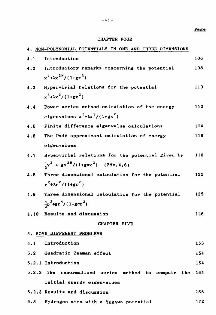
4. NON-POLYNOMIAL POTENTIALS IN ONE AND THREE DIMENSIONS
4.1
4.2
4.3
4.4
4.5
4.6
4.7
4.8
4.9
Introduction
Introductory remarks concerning the potential
X2 +Ax2N
/ (1+gx2
)
Hypervirial relations for the potential
x 2 + Ax 2 / ( 1 + gx 2 )
Power series method calculation of the energy
eigenvalues x2+~x2/(I+gX2)
Finite difference ei,envalue calculations
The Pade approximant calculation of ener,y
ei,envalues
Hypervirial relations for the potential given by
1 2 2M 2 "2x ;: gx / ( 1 +,ax) ( 2M= f 4 f 6 )
Three dimensional calculation for the potential
r 2+Xr2/(I+,r
2)
Three dimensional calculation for the potential
124 2 "2r ;:gr / (1+,ar )
4.10 Results and discussion
CHAPTER FIVE
5. SOME DIFFERENT PROBLEMS
5.1 Introduction
5.2 Quadratic Zeeaan effect
5.2.1 Introduction
106
108
110
112
114
116
118
122
125
126
153
154
154
5.2.2 The renormalised series method to compute the 164
initial energy ei,envalues
5.2.3 Results and discussion
5.3 Hydro,en atom with a Yukawa potential
166
172
-vii-
Page
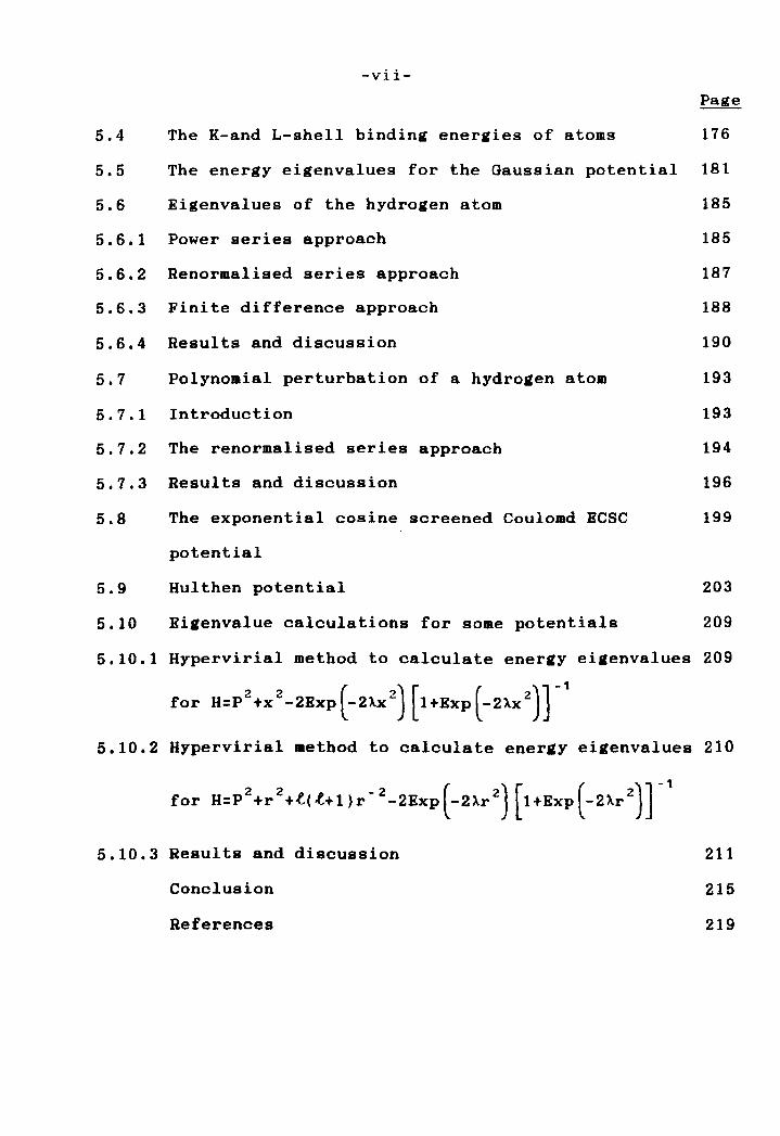
5.4 The K-and L-shell binding enereies of atoms 176
5.5 The energy eigenvalues for the Gaussian potential 181
5.6 Eigenvalues of the hydrogen atom 185
5.6.1 Power series approach 185
5.6.2 Renormalised series approach 187
5.6.3 Finite difference approach 188
5.6.4 Results and discussion 190
5.7 Polynomial perturbation of a hydrogen atom 193
5.7.1 Introduction 193
5.7.2 The renormalised series approach 194
5.7.3 Results and discussion 196
5.8 The exponential cosine screened Coulomd RCSC 199
5.9
5.10
potential
Hulthen potential
Bigenvalue calculations for soae potentials
203
209
5.10.1 Hypervirial method to calculate energy eigenvalues 209
for H:p2+x2_2BXP(_2xx2) [1+BXP (_2XX 2)]-1 5.10.2 Hypervirial method to calculate energy eigenvalues 210
for H:p2+r2+t(t+l)r-2_2ExP(_2Xr2) [1+ExP (_2xr 2)]-1 5.10.3 Results and discussion
Conclusion
References
211
215
219
-viii-
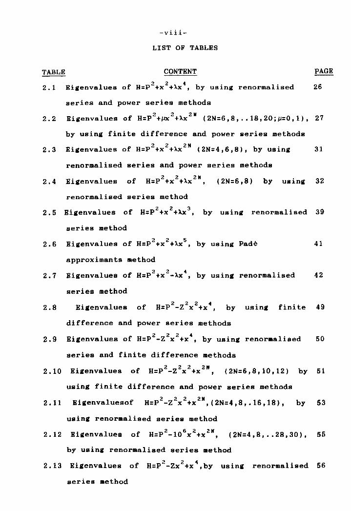
LIST OF TABLES
TABLE CONTENT PAGE
2.1 ., 2 4
Rigenvalues of H=P~+x +lx , by using renormalised 26
series and power series methods
2.2 Rigenvalues of H=p2+~2+1x2H (2N=6,8, .• 18,20;p=0,1), 27
by using finite difference and power series methods
2.3 Eigenvalues of H=p2+x2+1x2N (2N=4,6,8), by using 31
renormalised series and power series methods
2.4 Rigenvalues of 2 2 2N
H=P +x +lx , (2N=6,8) by using 32
renormalised series method
2.5 Rigenvalues of H=p2+x2+U3, by using renormalised 39
2.6
2.7
2.8
2.9
2.10
2.11
series method
2 2 5 Rigenvalues of H=P +x +u , by using Pade
approximants method
2 2 4 Rigenvalues of H=P +x -u , by using renormalised
series method
Eigenvalues of 222 4
H=P -Z x +x , by using finite
difference and power series methods
222 4 Rigenvalues of H=P -Z x +x , by using renormalised
series and finite difference methods
Rigenvalues of 2 2 2 2H H=P -Z x +x , (2N=6,8,10,12)
using finite difference and power series methods
Eigenvaluesof 2 2 2 2H H=P -Z x +x ,(2N=4,8,.16,18),
using renoraalised series method
by
by
41
42
49
50
61
53
2 12 R ' 1 of H_-P2_106x2+x2N, • 1genva ues (2N=4,8, •• 28,30), 55
by using renormalised series method
2.13 Rigenvalues of 2 2 4
H=P -Zx +x ,by using renormalised 56
series method
-x-
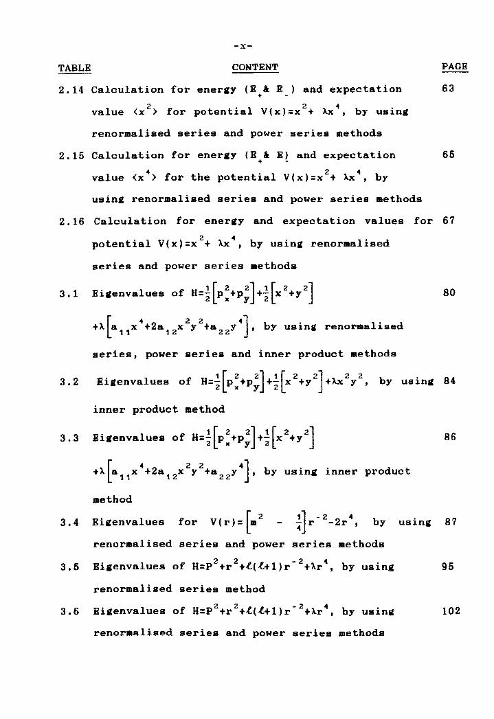
TABLB CONTENT PAGE
2.14 Calculation for energy (B & E ) and expectation 63 + -
value <x 2) for potential V(x)=x 2 + ~4, by using
renormalised series and power series methods
2.15 Calculation for energy (B & B) and expectation + -
65
value <x 4) for the potential V(x)=x 2 + ~x4, by
using renormalised series and power series methods
2. 16 Calculation for energy and expectation values for 67
potential V(x)=x2+ ~X4, by using renormalised
series and power series methods
80
series, power series and inner product methods
3.2 • 1 [2 2J 1 [2 2J 2 2 B1genvalues of H='2 px +Py +'2 x +y +~x y , by using 84
inner product method
3.3 Bigenvalues of H=i[p:+p;]+;[x2+y2] 86
+~[a11x4+2a12X2y2+a22y4], by using inner product
method
3.4 r 2 1] -2 4 Bigenvalues for V(r)=Lm 4 r -2r, by using 87
renormalised series and power series methods
3.5 • 2 2 -2 4
B1genvalues of H=P +r +~(~+l)r +~r, by using 95
renormalised series method
102
renormalised series and power series methods
-xi-
TABLE CONTENT PAGE
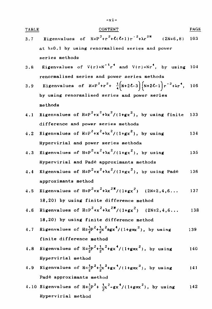
3.7 Eigenvalues of 2 2 - 2 2H H=P +r +t(t+1)r +Ar (2N=6,8) 103
at A=O.l by using renormalised series and power
series methods
3.8 Eigenvalues of - 1 4 4 V(r)=N rand V(r)=Nr , by using 104
renormalised series and power series methods
3.9 Eigenvalues of H=p2+r2+ ~(N+2t-3) (N+2t-l)r-2+Ar\ 105
by using renormalised series and power series
methods
4.1 2 2 2 2
Eigenvalues of H=P +x +AX /(1+ax ), by using finite 133
difference and power series methods
4.2 2 2 2 2 Eigenvalues of H=P +X +AX /(l+gx ), by using 134
Hypervirial and power series methods
4.3 2 2 2 2 Eigenvalues of H=P +x +AX /(l+gx ), by using 135
Hypervirial and Pade approximants methods
4.4 2 2 2 2 Eigenvalues of H=P +x +AX /(l+gx ), by using Pade 136
approximants method
4.5 . 2 2 2H 2 E1genvalues of H=P +x +Ax /(l+gx) (2N=2,4,6 .•• 137
18,20) by using finite difference method
4.6 • 2 2 2N 2 R1genvalues of H=P +x +AX /(1+gx) (2N=2,4,6 .•• 138
18,20) by using finite difference method
4.7 Eigenvalues of 1 2 1 2 4 2 H=2P +2x ±gx /(l+gax ), by using 139
finite difference method
4.8 Eigenvalues of 12124 2 H=2P +2x +gx /(l+gax ), by using 140
Hypervirial method
4.9 IUgenvalues of 12124 2 H=2P +2x +gx /(l+gax ), by using 141
Pade approximants method
1 2 1 2 4 2 4.10 Eigenvalues of H=-P + -2x -gx /(l+gax ), by using 142
2
Hypervirial method
-xii-
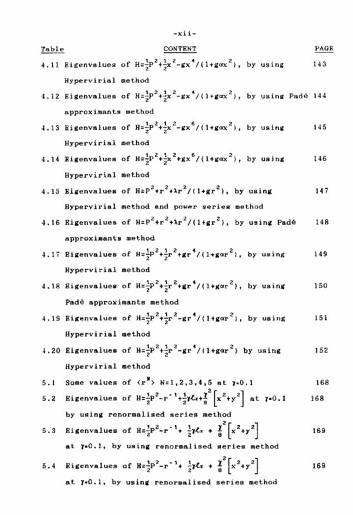
Table CONTENT PAGE
1 2 1 2 4 2 by using 143 4.11 Eigenvalues of H=-P +-x -gx /(1+gax ), 2 2
Hypervirial method
Eigenvalues 121 2
4.12 of H=-P +-x 2 2 4 2 -gx /(1+gax ), by using Pade 144
approximants method
1 2 1 2 6 2 ~.13 Eigenvalues of H=2P +2x -gx /(1+gax ), by using 145
Hypervirial method
1 2 1 2 6 2 4.14 Eigenvalues of H=2P +2x +gx /(l+gax ), by using 146
Hypervirial method
2 2 2 2 4.15 Eigenvalues of H=P +r +lr /(l+gr ), by using 147
Hypervirial method and power series method
2 2 2 2 4.16 Eigenvalues of H=P +r +lr /(1+gr ), by using Pade 148
approximants method
1 2 1 2 4 2 4.17 Eigenvalues of H=2P +2r +gr /(1+gar ), by using 149
Hypervirial method
1 2 1 2 4 2 4.18 Eigenvalues of H=2P +2r +gr /(1+gar ), by using 150
Pade approximants method
1 2 1 2 4 2 4.19 Eigenvalues of H=2P +2r -gr /(1+gar ), by using 151
Hypervirial method
1 2 1 2 4 2 4.20 Eigenvalues of H=2P +2r -gr /(l+gar ) by using
Hypervirial method
5.1 Some values of <rH) N=1,2,3,4,5 at 1:0.1
5.2 Eigenvalues of H=~p2_r-l+il.e.z+~2[x2+y2] at 1-0.1
by using renormalised series method
5.3 Eigenvalues of H=~p2_r-l+ ~l.e.z + ~2[x2+y2] at l a O.1, by using renormalised series method
4 · 1 f 1 2 -1 1 I' 12 [2 2] 5. Elgenva ues 0 H=2P -r + 21~z + 8 X +y
at 1-0.1, by using renormalised series method
152
168
168
169
169
-xiii-
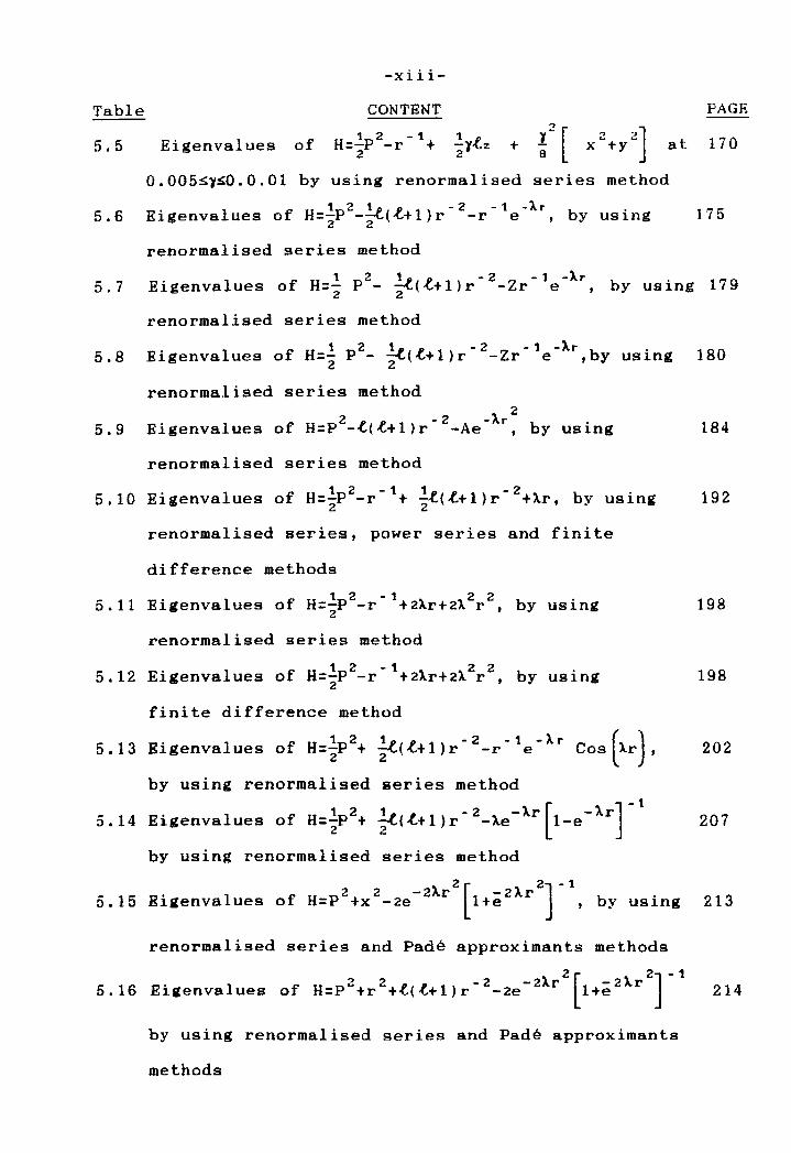
Table CONTENT PAGE
5.5 Eigenvalues of _"ta
2 [ ., 2J + x~+y at 170
O.005S1S0.0.01 by using renormalised series method
1 2 111 11 -2 -1 -Ar 5.6 Eigenvalues of H=2P -~(~+l)r -r e ,by using 175
renormalised series method
1 2 1" 11 -2 -1 -Ar 5.7 Eigenvalues of H=2 P - ~(~+l)r -Zr e ,by using 179
renormalised series method
1 2 1" 11 - 2 - 1 - Ar 5.8 Eigenvalues of H=z P - ~(~+l)r -Zr e ,by using 180
renormalised series method
5.9 2
2 "" - 2 - Ar Eigenvalues of H=P -~(~+1)r -Ae ,by using 184
renormalised series method
· f 1 2 -1 111 11 -2 5.10 E1genvalues 0 H=2P -r + 2~(~+1)r +Ar, by using 192
renormalised series, power series and finite
difference methods
· 1 2 -1 2 2 5.11 E1genvalues of H=2P -r +2Ar+2A r , by using 198
renormalised series method
· 1 2 -1 2 2 5.12 E1genvalues of H=2P -r +2Ar+2A r , by using 198
finite difference method
5.13 · f 1 Z 111 11 -2 -1 -Ar () E1genvalues 0 H=2P + ~(~+l)r -r e Cos lr , 202
by using renormalised series method
5.14 · 1 f 1 Z 1"" - Z -lr [ -lr] - 1 E1genva ues 0 H=2P + ~(~+l)r -le 1-e 207
by using renormalised series method
· 2 Z -ZAr2[ _2lr2]-1 5.15 E1genvalues of H=P +x -2e l+e , by using 213
renormalised series and Pade approximants methods
5.16 Eigenvalues of H=p2+r2+t(t+l)r-2_ze-2Ar2[1+e2lrZ]-1 214
by using renormalised series and Pade approximants
methods
1.1 Introductory remarks
-1-
CHAPTER ONE
Introduction
The aim of this work is to use numerical techniques to
compute the energy eigenvalues for one-particle Schrbdinger
equations in one, two, three and (N=1,2,3,4, ..... 1000)
dimensions, for a large number of potentials with different
forms, as we shall see later. We face convergence
di fficul ties in dealing wi th perturbation methods. However,
there are an extensive range of techniques in the
mathematical literature to deal with divergence problem e.g
renormalised series, Pade approximants and the Aitken
procedure. We wish to point out that we overcome the
convergence problem, to ensure that our results are correct.
by using the renormalised constant (K) which is given in the
review of Killingbeck [12,1980;14,1982]. The renormalization
constant (K) plays an important role in the convergence
aspects of the calculations which are investigated in this
work. Also, Pade approximants and the Aitken procedure have
been used to calculate the energy eigenvalues for some
problems. The resul ts are compared wi th those produced by
different methods which can be used to calculate energies for
the same perturbed potentials.
1.2 Summary of selected previous and present work for chapter
two
Bender and Wu [1,1969] have calculated 75 terms of the
ground state energy perturbation series for the 2N=4 case of
the anharmonic oscillator defined by the Hamiltonian
-2-
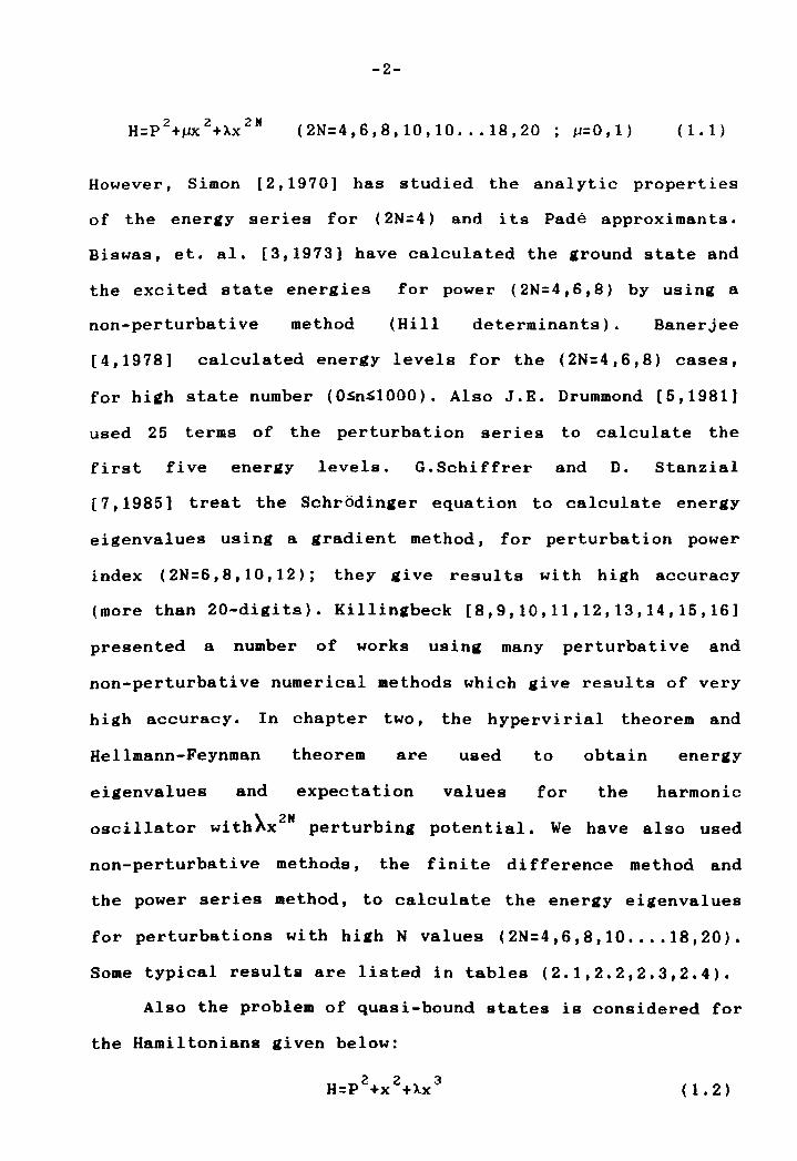
(2N=4,6,8,10,10 ... 18,20 11= 0, 1 ) ( 1. 1 )
However, Simon [2,1970] has studied the analytic properties
of the energy series for (2N=4) and its Pade approximants.
Biswas, et. al. [3,1973] have calculated the ground state and
the excited state energies for power (2N=4,6,8) by using a
non-perturbative method (Hill determinants). Banerjee
[4,1978] calculated energy levels for the (2N=4,6,8) cases,
for high state number (O~n~1000). Also J.B. Drummond [5,1981]
used 25 terms of the perturbation series to calculate the
first five energy levels. G.Schiffrer and D. Stanzial
[7,1985] treat the Schrodinger equation to calculate energy
eigenvalues using a gradient method, for perturbation power
index (2N=6,8, 10, 12); they give results with high accuracy
(more than 20-digits). Killingbeck [8,9,10,11,12,13,14,15,16]
presented a number of works using many perturbative and
non-perturbative numerical methods which give results of very
high accuracy. In chapter two, the hypervirial theorem and
Hellmann-Feynman theorem are used to obtain energy
eigenvalues and expectation values for the harmonic
oscillator wi th).x2N
perturbing potential. We have also used
non-perturbative methods, the finite difference method and
the power series method, to calculate the energy eigenvalues
for perturbations with high N values (2N=4,6,8,10 •••• 18,20).
Some typical results are listed in tables (2.1,2.2,2.3,2.4).
Also the problem of quasi-bound states is considered for
the Hamiltonians given below:
223 H=P +x +>"x ( 1. 2)
-3-
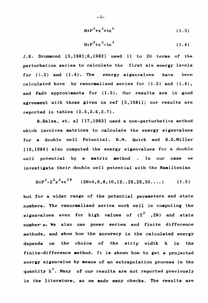
2 2 5 H=P +x +>..x ( 1. 3)
2 2 4 H=P +x ->..x ( 1. 4)
J.E. Drummond [5,1981;6,1982] used 11 to 20 terms of the
perturbation series to calculate the first six energy levels
for (1.2) and (1.4). The energy eigenvalues have been
calculated here by renormalised series for (1.2) and (1.4),
and Pade approximants for (1.3). Our resul ts are in good
agreement with those given in ref [5,1981]; our results are
reported in tables (2.5,2.6,2.7).
R.Balsa, et. al [17,1983] used a non-perturbative method
which involves matrices to calculate the energy eigenvalues
for a double well Potential. R.M. Quick and H.G.Miller
[18,1984] also computed the energy eigenvalues for a double
well potential by a matrix method In our case we
investigate their double well potential with the Hamiltonian
H P2 z2 2 2N = - x +x (2N=4,6,8,10,12 •. 26,28,30 .••• ) ( 1. 5 )
but for a wider range of the potential parameters and state
numbers. The renormalised series work well in computing the
eigenvalues even for high values of (Z2 ,2N) and state
number'~' We also use power series and finite difference
methods, and show how the accuracy in the calculated energy
depends on the choice of the strip width h in the
finite-difference method. It is shown how to get a projected
energy eigenvalue by means of an extrapolation process in the
quantity h 2• Many of our results are not reported previously
in the 1 i tera ture, so we made many checks. The resul ts are
-4-
shown in tables (2.8 to 2.13).
1.3 Summary of selected previous and present work for chapter
three
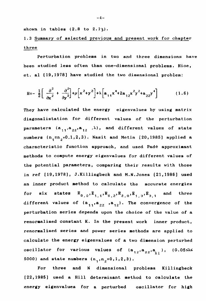
Perturbation problems in two and three dimensions have
been studied less often than one-dimensional problems. Hioe,
et. al [19,1978] have studied the two dimensional problem:
1 [a 2 02J [2 2J [4 2 2 4J H=- x -- + -- +IJ x +y +>.. a x +2a x y +a y ~ ax2 oy2 11 12 22
( 1. 6)
They have calculated the ener&y eigenvalues by usin& matrix
diagonalistation for different values of the perturbation
parameters (a11,a22,a12 ,>..), and different values of state
numbers (n 1=n z=0,1,2,3). Nasit and Metin [20,1985) applied a
characteristic function approach, and used Pad~ approximant
methods to compute energy eigenvalues for different values of
the potential parameters, comparing their results with those
in ref [19,1978], J.Killingbeck and M.N.Jones [21,1986] used
an inner product method to calculate the accurate energies
for six states E ,E ,E ,E ,E ,E 0,0 1,1 0,2 20 1,3 3,1 and three
different values of (a 11 ,a 22 ,a 12 ). The convergence of the
perturbation series depends upon the choice of the value of a
renormalised constant K. In the present work inner product,
renormalised series and power series methods are applied to
calculate the energy eigenvalues of a two dimension perturbed
oscillator for various values of (0. 05~~
5000) and state numbers (n 1 ,n 2=0,1,2,3).
For three and N dimens i onal problems Killingbeck
[22,1985] used a Hill determinant method to calculate the
energy eigenvalues for a perturbed oscillator for high
-5-
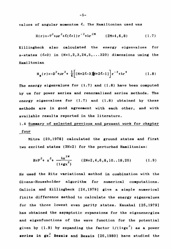
values of angular momentum ~. The Hamiltonian used was
2 2 -2 2M H(r)=-V +~r +~(~+l)r +Ar (2M:4,6,8) ( 1. 7)
Killingbeck also calculated the energy eigenvalues for
s-states (~O) in (N=1,2,3,24,5, ... 320) dimensions using the
Hamiltonian
( 1 .8)
The energy eigenvalues for (1.7) and (1.8) have been computed
by us for power series and renormalised series methods. The
energy eigenvalues for (1.7) and (1.8) obtained by these
methods are in good agreement with each other, and wi th
available results reported in the literature.
1.4 Summary of selected previous and present work for chapter
four
Mitra [23,1978) calculated the ground states and first
two excited states (2N=2) for the perturbed Hamiltonian:
(2N=2,4,6,8,10 .. 18,20) (1. 9)
He used the Ritz variational method in combination with the
Givens-Householder algorithm for numerical computations.
Galicia and Killingbeck [24,1979] give a simple numerical
finite difference method to calculate the energy eigenvalues
for the three lowest even parity states. Kaushal [25,1979]
has obtained the asymptotic expansions for the eigenenergies
and eigenfunctions of the wave function for the potential
2 given by (1.9) by expanding the factor l/(l+gx ) as a power
2 aeriea in gx. Bessis and Bessis [26,1980] have studied the
-6-
same problem by taking advantage of a two parameter (A and g)
scale transformation, and Hautot [27,1981] has used a Hill
determinant method for the potential. Lai and Lin [28,1982]
have applied the Hellmann-Feynman theorem and hypervirial
theorem to obtain the perturbation series for the energy
eigenvalues; they have employed the PadA approximant method
to sum the energy series. Their results, however, require the
asymptotic expansion of the factor 1/(1+gx 2) as a power
series in gX 2, which is valid for low values of g~2 only. On
the other hand, V. Fack and Vanden Berghe [29,1985] used a
finite difference method in combination with matrix
diagonalisation for numerical computation, and transformed
the Schrodinger equation into an algebraic eigenvalue problem
involving special forms of matrix. They calculated the energy
eigenvalues for various values of g and A and strip width h
and compared their results wi th those of [28,1982]. This
problem has received great attention from us, and we used
perturbative and non-perturbative methods to attack the
problem. We determined the energy eigenvalues for various
values of the state number (n), and over a wide range of
values of A,g and power index (2N:2,4,6, •. 18,20).
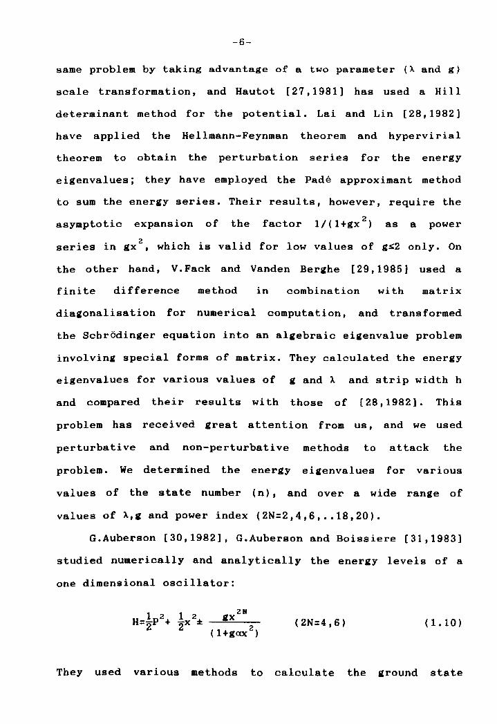
G.Auberson [30,1982], G.Auberson and Boissiere [31,1983]
studied numerically and analytically the energy levels of a
one dimensional oscillator:
(2N:4,6) (1.10)
They used various methods to calculate the ground state
-7-
energy eigenvalues for different values of g and a, for the
case 2N=4. We calculate in the present work energies for the
ground state and many excited states, for different values of
g and a and for (2N:4,6), using the renormalised series and
finite difference methods. The results are compared in tables
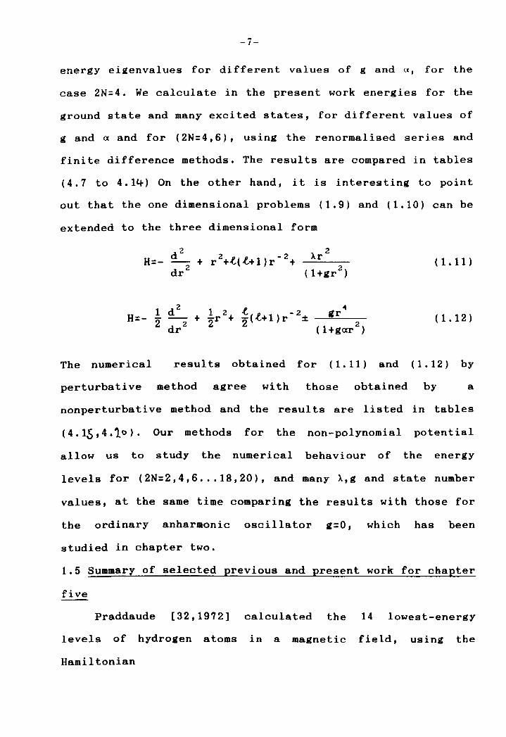
(4.7 to 4.14) On the other hand, it is interesting to point
out that the one dimensional problems (1.9) and (1.10) can be
extended to the three dimensional form
(1.11)
1 d2
lr2+.t p -2 gr4
H:- 2" dr 2 + 2 2"(~+l)r ± 2 (1+gar )
(1.12)
The numerical results obtained for (1.11) and (1.12) by
perturbative method agree with those obtained by a
nonperturbative method and the results are listed in tables
(4.15,4.10). Our methods for the non-polynomial potential
allow us to study the numerical behaviour of the energy
levels for (2N:2,4,6 .•. 18,20), and many A,g and state number
values, at the same time comparing the results with those for
the ordinary anharmonic oscillator g:O, which has been
studied in chapter two.
1.5 Summary of selected previous and present work for chapter
five
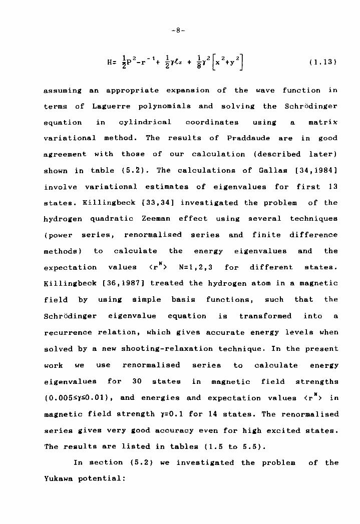
Praddaude [32,1972] calculated the 14 lowest-energy
levels of hydrogen atoms in a magnetic field, using the
Hamiltonian
-8-
1 2 -1 1 1 2 [2 2] H= 2P -r + 21~Z + 81 x +y (1.13)
assuming an appropriate expansion of the wave function in
terms of Laguerre polynomials and solving the Schrodinger
equation
variational
in cylindrical coordinates using
method. The resul ts of Praddaude
a
are
matrix
in good
agreement with those of our calculation (described later)
shown in table (5.2). The calculations of Gallas [34,1984]
involve variational estimates of eigenvalues for first 13
states. Killingbeck [33,34] investigated the problem of the
hydrogen quadratic Zeeman effect using several techniques
(power
methods)
series, renormalised series and finite difference
to calculate the energy eigenvalues and the
expectation values <rH) N=1,2,3 for different states.
Killingbeck [36,1987] treated the hydrogen atom in a magnetic
field by using simple basis functions, such that the
Schrbdinger eigenvalue equation is transformed into a
recurrence relation, which gives accurate energy levels when
solved by a new shooting-relaxation technique. In the present
work we use renormalised series to calculate eneriY
eigenvalues for 30 states in magnetic field strengths
(0.005~1~O.01), and energies and expectation values <rH) in
magnetic field strength 1=0.1 for 14 states. The renormalised
series gives very good accuracy even for high excited states.
The results are listed in tables (1.5 to 5.5).
In section (5.2) we investigated the problem of the
Yukawa potential:
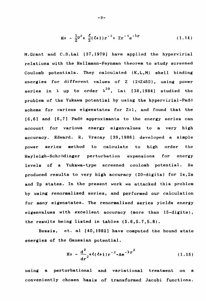
-9-
1 2 .t p - 2 - 1 - Ar H= - 2V + 2(~+1)r + Zr e (1. 14)
M.Grant and C.S.Lai [37,1979] have applied the hypervirial
relations with the Hellmann-Feynman theorem to study screened
Coulomb potentials. They calculated (K,L,M) shell binding
energies for different values of Z (2~Z~50), using power
series in A up to order A20, Lai [38,1984] studied the
problem of the Yukawa potential by using the hypervirial-Pade
scheme for various eigenstates for Z=l, and found that the
[6,6] and [6,7] Pade approximants to the energy series can
account for various energy eigenvalues to a very high
accuracy. Edward. R. Vrscay [39,1986] developed a simple
power series method to calculate to high order the
Rayleigh-Schrbdinger perturbation expansions for energy
levels of a Yukawa-type screened coulomb potential. He
produced results to very high accuracy (20-digits) for ls,2s
and 2p states. In the present work we attacked this problem
by using renormalised series, and performed our calculation
for many eigenstates. The renormalised series yields energy
eigenvalues with excellent accuracy (more than 15-digi ts) ,
the results being listed in tables (5.6,5.7,5.8).
Bessis, et. al [40,1982] have computed the bound state
energies of the Gaussian potential.
2 2 d g p - 2 - Ar H= - -- +~(~+l)r -Ae dr 2 (1.15)
using a perturbational and variational treatment on a
conveniently chosen basis of transformed Jacobi functions.
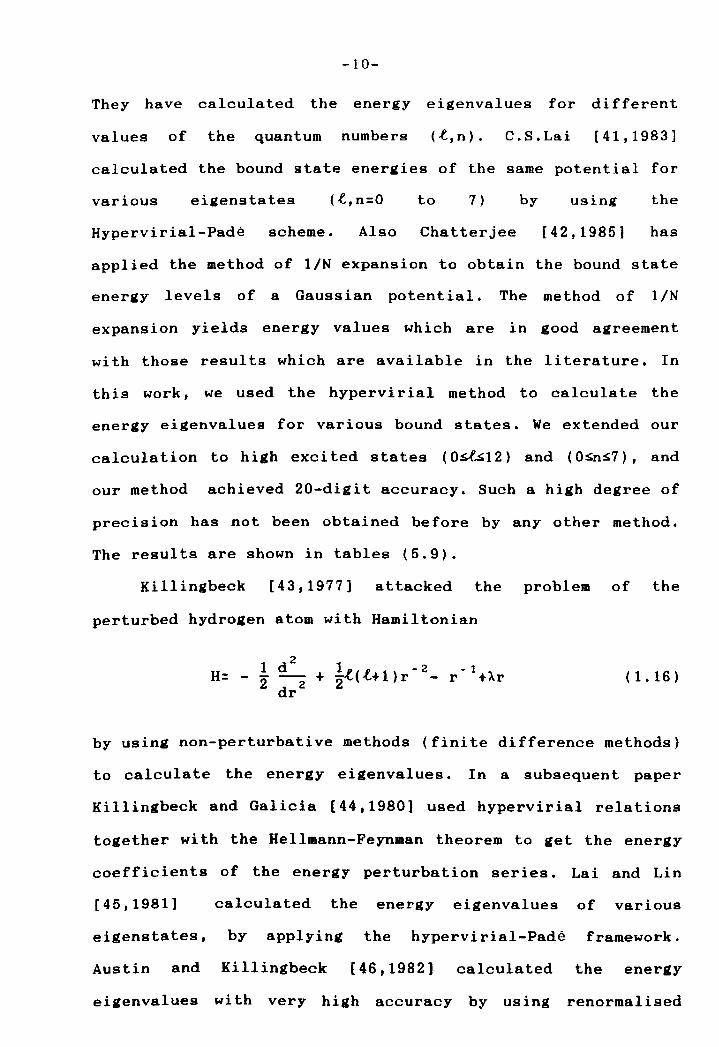
-10-
They have calculated the energy eigenvalues for different
values of the quantum numbers (t,n). C.S.Lai [41,1983]
calculated the bound state energies of the same potential for
various eigenstates (t,n:O to 7) by using the
Hypervirial-Pade scheme. Also Chatterjee [42,1985] has
applied the method of 1/N expansion to obtain the bound state
energy levels of a Gaussian potential. The method of 1 IN
expansion yields energy values which are in good agreement
with those results which are available in the literature. In
this work, we used the hypervirial method to calculate the
energy eigenvalues for various bound states. We extended our
calculation to high excited states (O~12) and (0~n~7), and
our method achieved 20-digit accuracy. Such a high degree of
precision has not been obtained before by any other method.
The results are shown in tables (5.9).
Killingbeck [43,1977] attacked the problem of the
perturbed hydrogen atom with Hamiltonian
1 d 2 1 ... "" -2 -1 H= - 2 dr 2 + ~(~+l)r - r +Ar ( 1. 16 )
by using non-perturbative methods (finite difference methods)
to calculate the energy eigenvalues. In a subsequent paper
Killingbeck and Galicia [44,1980] used hypervirial relations
together with the Hellmann-Feynman theorem to get the energy
coefficients of the energy perturbation series. Lai and Lin
[45,1981] calculated the energy eigenvalues of various
eigenstates, by applying the hypervirial-Pade framework.
Austin and Killingbeck [46,1982] calculated the energy
eigenvalues wi th very high accuracy by using renormalised
-11-
series. We calculated the energy eigenvalues for this problem
by using power series, finite difference and renormal ised
series methods. The results produced by these methods are in
good agreement with each other. The results are listed in
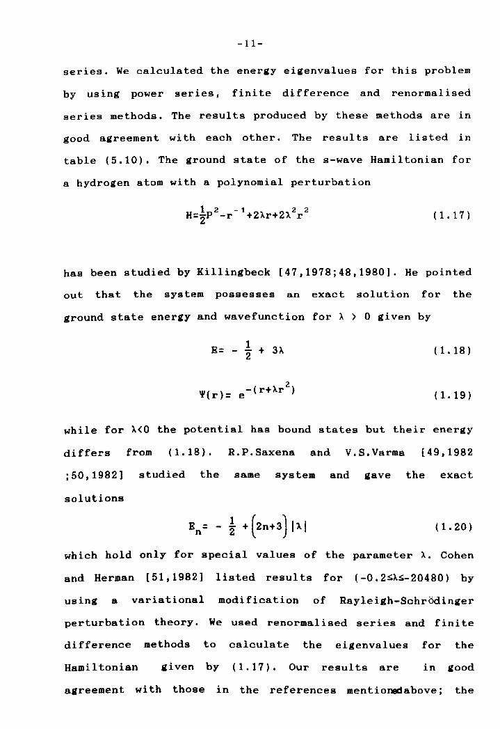
table (5.10). The ground state of the s-wave Hamiltonian for
a hydrogen atom with a polynomial perturbation
(1.17)
has been studied by Killingbeck [47,1978;48,1980]. He pointed
out that the system possesses an exact solution for the
ground state energy and wavefunction for A > 0 given by
B= - 1 + 3X 2
'I'(r)= 2 - (r+Xr ) e
(1.18)
(1.19)
while for X<O the potential has bound states but their energy
differs from (1.18). R.P.Saxena and V.S.Varma [49,1982
;50,1982] studied the same system and gave the exact
solutions
( 1. 20)
which hold only for special values of the parameter X. Cohen
and Herman [51,1982] listed results for (-0.2~X~-20480) by
using a variational modification of Rayleigh-Schrbdinger
perturbation theory. We used renormalised series and finite
difference methods to calculate the eigenvalues for the
Hamiltonian given by (1.17). Our results are in lood
agreement with those in the references ment iolW:l above ; the
-12-
results are reported in tables (5.11,5.12).
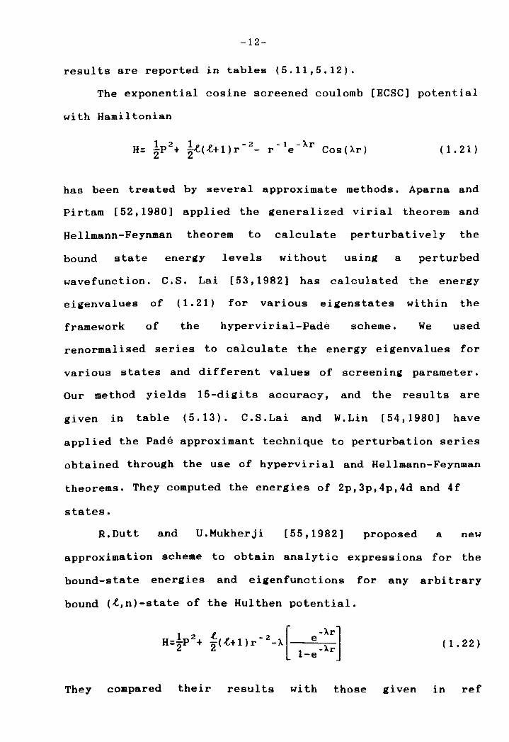
The exponential cosine screened coulomb [ECSC] potential
with Hamiltonian
1 2 1" - 2 - 1 - Ar H= 2P + ~(~+1)r - r e Cos(Ar) (1.21)
has been treated by several approximate methods. Aparna and
Pirtam [52,1980] applied the generalized virial theorem and
Hellmann-Feynman theorem to calculate perturbatively the
bound state energy levels without using a perturbed
wavefunction. C.S. Lai [53,1982] has calculated the energy
eigenvalues of (1.21) for various eigenstates within the
framework of the hypervirial-Pade scheme. We used
renormalised series to calculate the energy eigenvalues for
various states and different values of screening parameter.
Our method yields 15-digits accuracy, and the results are
given in table (5.13). C.S.Lai and W.Lin [54,1980] have
applied the Pade approximant technique to perturbation series
obtained through the use of hypervirial and Hellmann-Feynman
theorems. They computed the energies of 2p,3p,4p,4d and 4f
states.
R.Dutt and U.Mukherji [55,1982] proposed a new
approximation scheme to obtain analytic expressions for the
bound-state energies and eigenfunctions for any arbitrary
bound (-t,n)-state of the Hulthen potential.
( 1. 22)
They compared their results with those given in ref
-13-
[22,1982]. We used the renormalised series to calculate the
energy eigenvalues for (1.22) for various values of A and for
high excited states (2p to Bh). The renormalised series give
high accuracy (15-digits).
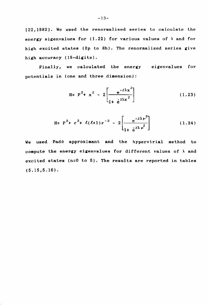
Finally, we calculated the energy
potentials in (one and three dimension):
H= p2+ 2 x
2 2 ~ g -2 H= P + r + ~(~+I)r -
eigenvalues for
(1. 23)
( 1. 24 )
We used Pade approximant and the hypervirial method to
compute the energy eigenvalues for different values of A and
excited states (n=O to 5). The results are reported in tables
(5.15,5.16).
-14-
CHAPTER TWO
ONE-DIMENSIONAL MODEL PROBLEMS
2.1 Numerical calculation for H:p2+px2+Ax2N
(2N:4,6,8,10 •. 18,20)
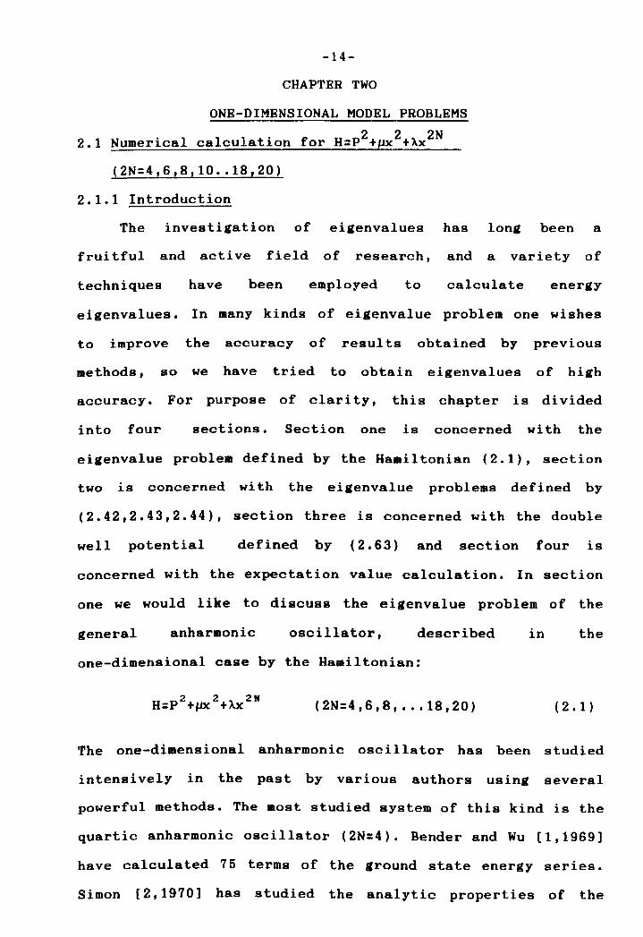
2.1.1 Introduction
The investigation of eigenvalues has long been a
fruitful and active field of research, and a variety of
techniques have been employed to calculate energy
eigenvalues. In many kinds of eigenvalue problem one wishes
to improve the accuracy of results obtained by previous
methods, so we have tried to obtain eigenvalues of high
accuracy. For purpose of clari ty, this chapter is divided
into four sections. Section one is concerned with the
eigenvalue problem defined by the Hamiltonian (2.1), section
two is concerned wi th the eigenvalue problems defined by
(2.42,2.43,2.44), section three is concerned with the double
well potential defined by (2.63) and section four is
concerned with the expectation value calculation. In section
one we would like to discuss the eigenvalue problem of the
general anharmonic oscillator, described in the
one-dimensional case by the Hamiltonian:
(2N:4,6,8, •.. 18,20) ( 2 • 1 )
The one-dimensional anharmonic oscillator has been studied
intensively in the past by various authors using several
powerful methods. The most studied system of this kind is the
quartic anharmonic oscillator (2N:4). Bender and Wu [1,1969]
have calculated 75 terms of the ground state energy series.
Simon [2,1970] has studied the analytic properties of the
-15-
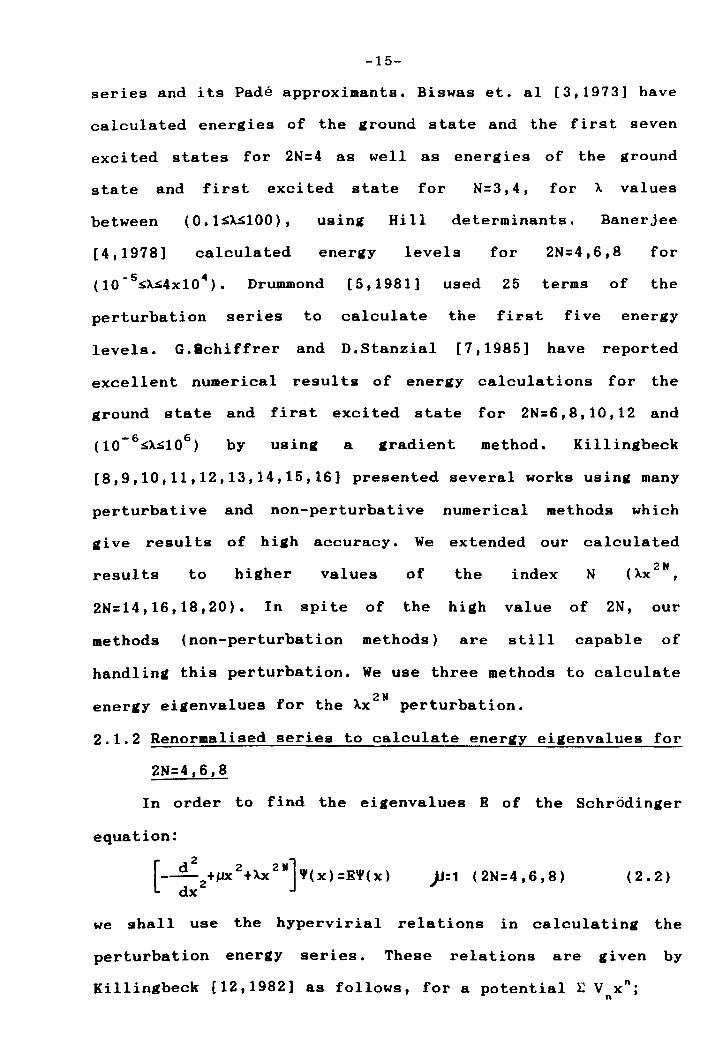
series and its Pade approximants. Biswas et. al [3,1973] have
calculated energies of the ground state and the first seven
exci ted states for 2N=4 as well as energies of the ground
state and first excited state for N=3,4, for ~ values
between (0.1~~100), using Hill determinants. Banerjee
[4,1978] calculated energy levels for 2N=4,6,8 for
(10-5~~4xl04). Drummond [5,1981] used 25 terms of the
perturbation series to calculate the first five energy
levels. G.lchiffrer and D.Stanzial [7,1985] have reported
excellent numerical results of energy calculations for the
ground state and first excited state for 2N=6, 8,10,12 and
by using a gradient method. Killingbeck
[8,9,10,11,12,13,14,15,16] presented several works using many
perturbative and non-perturbative numerical methods which
give results of high accuracy. We extended our calculated
results to higher values of the index N
2N=14,16,18,20). In spite of the high value of 2N, our
methods (non-perturbation methods) are still capable of
handling this perturbation. We use three methods to calculate
energy eigenvalues for the ~X2N perturbation.
2.1.2 Renormalised series to calculate energy eigenvalues for
2N=4,6,8
In order to find the eigenvalues B of the Schr6dinger
equation:
)J:1 (2N=4,6,8) ( 2 • 2 )
we shall use the hypervirial relations in calculating the
perturbation energy series. These relations are given by
Killingbeck [12,1982] as follows, for a potential E V xn; n
-16-
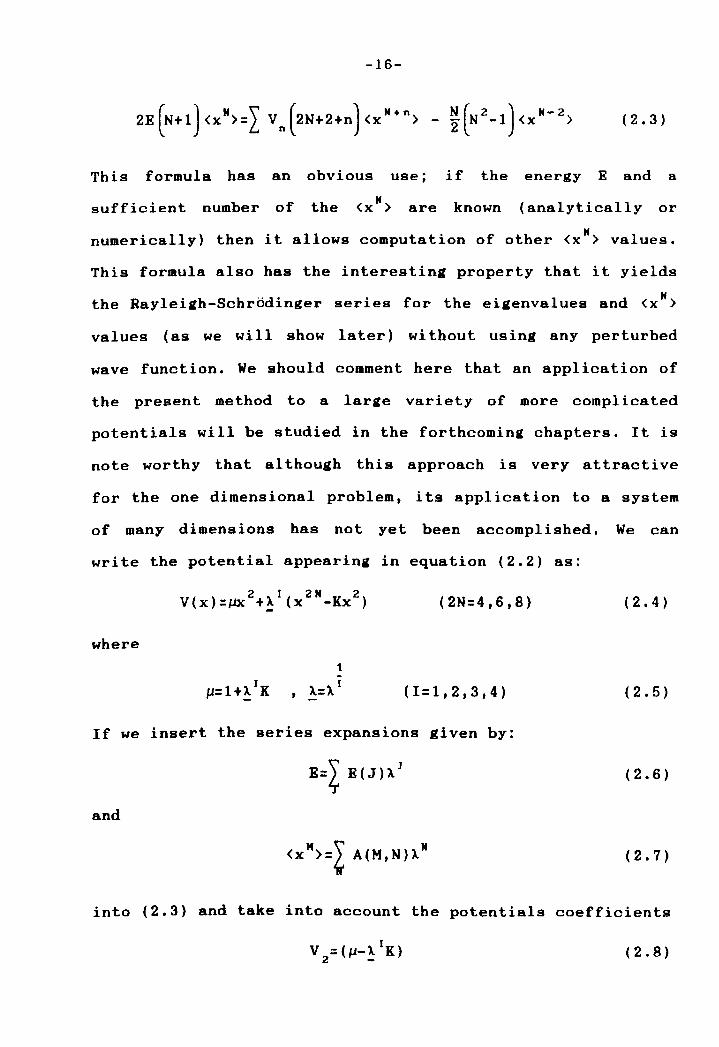
( 2 .3)
This formula has an obvious use; if the energy E and a
sufficient number of the <x M) are known (analytically or
numerically) then it allows computation of other <x M) values.
This formula also has the interesting property that it yields
the Rayleigh-Schrodinger series for the eigenvalues and <xM)
values (as we will show later) without using any perturbed
wave function. We should comment here that an application of
the present method to a large variety of more complicated
potentials will be studied in the forthcoming chapters. It is
note worthy that although this approach is very attractive
for the one dimensional problem, its application to a system
of many dimensions has not yet been accomplished. We can
write the potential appearing in equation (2.2) as:
2 I 2N 2 V(x)=gK +~ (x -Kx) (2N=4,6,8) ( 2 . 4 )
where
1
I I 1-/= 1 + ~ K , "'= '" (1=1,2,3,4) ( 2 . 5 )
If we insert the series expansions given by:
(2.6)
and
M \' N <x >={r A(M,N)'" ( 2 • 7 )
into (2.3) and take into account the potentials coefficients
I V = (1-1- '" K)
2 -(2.8)
V :",1 2n+2 -
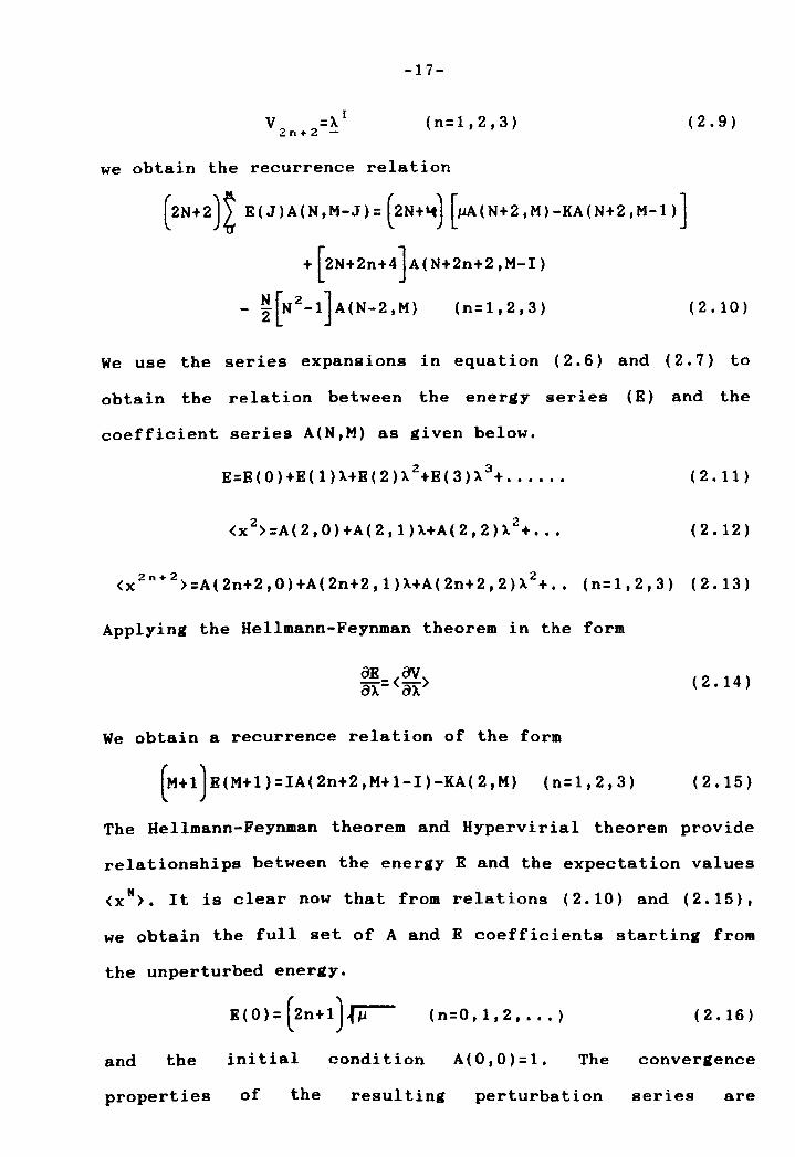
-17-
(n=I,2,3)
we obtain the recurrence relation
( 2 N + 2 ) ~ E ( J ) A ( N , M - J ) : (2 N + ... ) [/-LA ( N + 2 , M ) - KA ( N + 2 , M-I ) ]
+ [2N+2n+4]A(N+2n+2,M-I)
- ~[N2-1]A(N-2,M) (n=1,2,3)
( 2 .9)
(2.10)
We use the series expansions in equation (2.6) and (2.7) to
obtain the relation between the energy series (E) and the
coefficient series A(N,M) as given below.
2 3 E:E(0)+E(I)"'+E(2)'" +E(3)'" + ••.•.. (2.11)
2 2 <x >=A(2,0)+A(2,1)"'+A(2,2)'" + ••• (2.12)
2n+2 0 (2 2 <x >=A(2n+2, )+A n+2,1)"'+A(2n+2,2)'" + •• (n:1,2,3) (2.13)
Applying the Hellmann-Feynman theorem in the form
(2.14)
We obtain a recurrence relation of the form
(M+l)E(M+l):IA(2n+2,M+I-I)-KA(2,M) (n:l,2,3) (2.15)
The Hellmann-Feynman theorem and Hypervirial theorem provide
relationships between the energy E and the expectation values
<x M>. It is clear now that from relations (2.10) and (2.15),
we obtain the full set of A and E coefficients starting from
the unperturbed energy.
(n:O, 1,2, •.• ) (2.16)
and the initial condition A(O,0)=1. The convergence
properties of the resulting perturbation series are
-18-
controlled by varying K.
The renormalised series work very well for the quartic
perturbation (2N:4,I:1). The interesting point about this
approach for (2N:6,8) calculations is that the accuracy
varies with the power (I). We use this modified (variable I)
technique to perform more accurate calculations. These
calculations by the renormalised series technique become
progressively more difficul t as N increases; thus one must
keep in mind that we can partly overcome this difficulty by
introducin" A I. The primary motivation of this idea is to
improve the accuracy of our eigenvalues results, using a very
simple extension of the original renormalised series
technique. It is important to point out that the effect of
varying K the renormalised constant, is to allow us to
obtain results of high accuracy. The best K values in this
calculation have been obtained by numerical search, so our
calculation reveals the importance of finding the best values
of the renormalised constant. The convergence rate decreases
remarkably when X and 2N increase. Problems with computer
overflow were avoided by using the definition
N A(N,M)~2 A(N,M). The renormalised technique has been used by
Killingbeck for many eigenvalues problems, and has provided
an excellent way to overcome divergence problems as well as
to obtain eigenvalues with very high accuracy.
2.1.3 Finite-difference eigenvalue calculations
The finite-difference approach is a nonperturbative
method capable of arbitrarily high accuracy. This method has
been described by Killingbeck in reference [12,1982]. We will
only mention the essential feature here; the reader
-19-
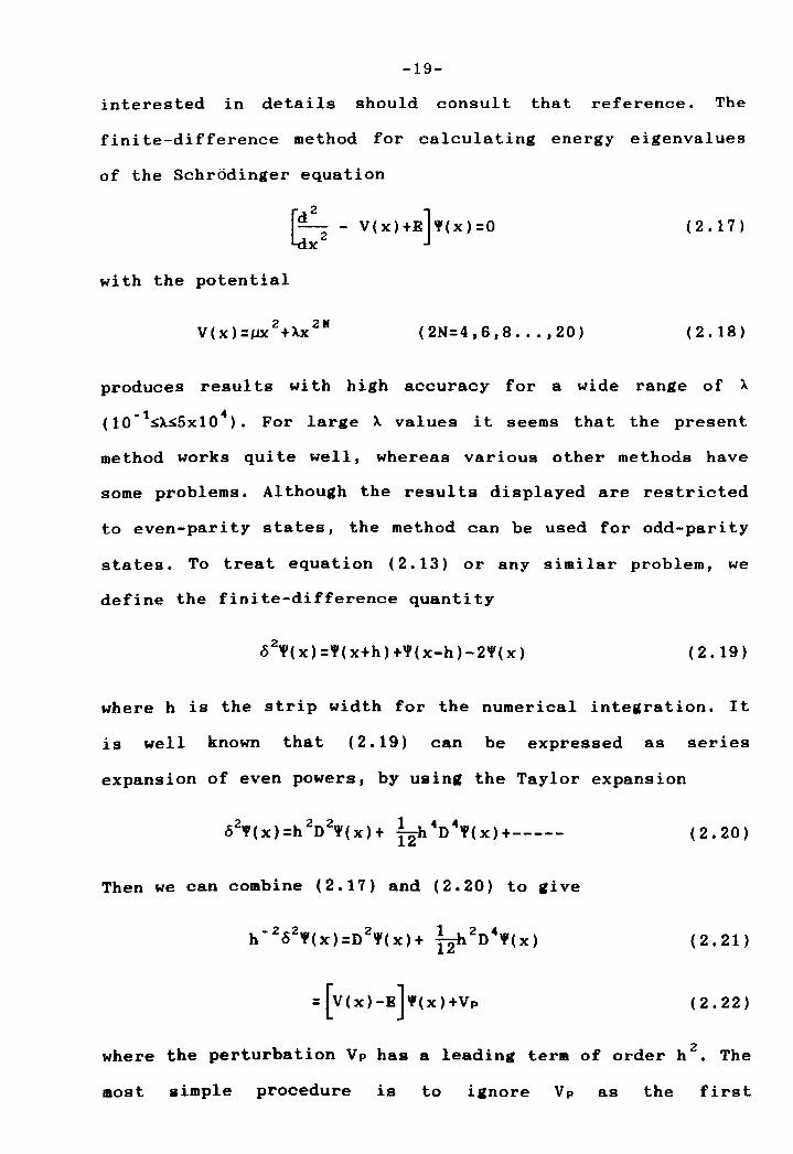
interested in details should consult that reference. The
fini te-difference method for calculating energy eigenvalues
of the Schrodinger equation
r~X22 ] ltt - V(x)+E 'I'(x)=O ( 2 . 17)
with the potential
2 2N V(x)=1JX +).x (2N=4,6,8 .•• ,20) (2.18)
produces results wi th high accuracy for a wide range of A.
(10-1~.s;5x1004). For large A. values it seems that the present
method works quite well, whereas various other methods have
some problems. Although the results displayed are restricted
to even-parity states, the method can be used for odd-parity
states. To treat equation (2.13) or any similar problem, we
define the finite-difference quantity
(2.19)
where h is the strip width for the numerical integration. It
is well known that (2.19) can be expressed as series
expansion of even powers, by using the Taylor expansion
222 144 6 'I'(x)=h D 'I'(x)+ 12h D ,(x)+----- (2.20)
Then we can combine (2.17) and (2.20) to give
-2 2 2 1 2 4 h 6 '(x)=D '(x)+ f2b D '(x) (2.21)
= [V(X)-E ]'I'(X)+VP (2.22)
where the perturbation VP has a leading term of order h 2• The
most simple procedure is to ignore Vp as the first
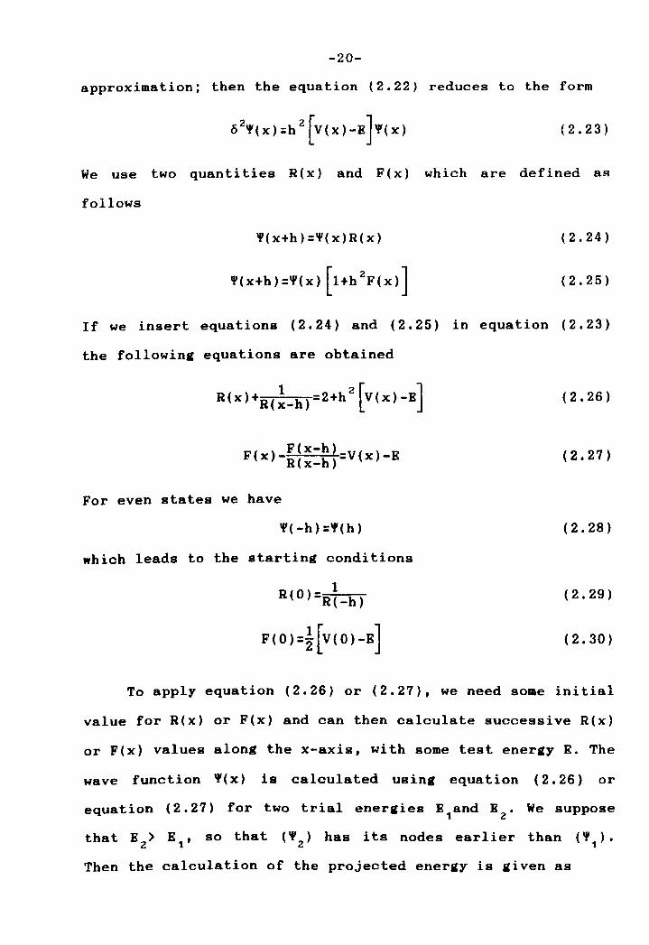
-20-
approximation; then the equation (2.22) reduces to the form
(2.23)
We use two quantities R(x) and F(x) which are defined as
follows
'(x+h)='(x)R(x) (2.24)
(2.25)
If we insert equations (2.24) and (2.25) in equation (2.23)
the following equations are obtained
F(x-h) F(x)-R(x_h)=V(x)-E
For even states we have
'I'(-h)='I'(h)
which leads to the starting conditions
1 R(O)=R(_h)
F (0) =l [V (0) -EJ
(2.26)
(2.27)
(2.28)
(2.29)
(2.30)
To apply equation (2.26) or (2.27), we need some initial
value for R(x) or F(x) and can then calculate successive R(x)
or F(x) values along the x-axis, with some test energy E. The
wave function 'I'(x) is calculated using equation (2.26) or
equation (2.27) for two trial energies E and E • We suppose 1 2
that E2> E 1 , so that ('1'2) has its nodes earlier than ('1)'
Then the calculation of the projected energy is given as
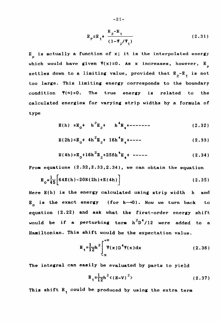
E =E + p t
-21-
E -E 2 1
(1-'1' 1" ) 2 1
( 2 • 31)
E is actually a function of x; it is the interpolated energy p
which would have given '1'( x) =0. As x increases, however, E p
settles down to a limiting value, provided that E -E is not 2 t
too large. This limiting energy corresponds to the boundary
condition '(00)=0. The true energy is related to the
calculated energies for varying strip widths by a formula of
type
4 h E +-------4
2 4 E(4h)=E +16h E +256h E + -----
024
(2.32)
(2.33)
(2.34)
From equations (2.32,2.33,2.34), we can obtain the equation
(2.35)
Here E(h) is the energy calculated using strip width hand
Eo is the exact energy (for h~). Now we turn back to
equation (2.22) and ask what the first-order energy shift
would be if a perturbing were added to a
Hamiltonian. This shift would be the expectation value.
1 2J+00 4 E t =f2b 'l'(x)D 'l'(x)dx
-00
(2.36)
The integral can easily be evaluated by parts to yield
(2.37)
This shift Et could be produced by using the extra term
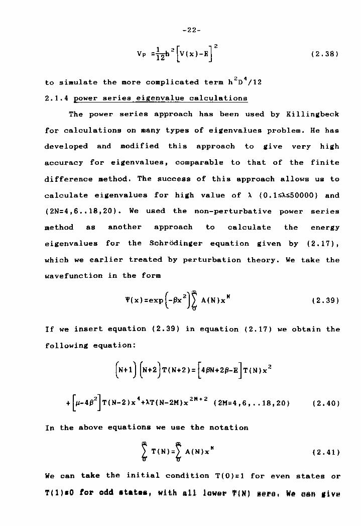
-22-
(2.38)
to simulate the more complicated term h2D4/12
2.1.4 power series eigenvalue calculations
The power series approach has been used by Killingbeck
for calculations on many types of eigenvalues problem. He has
developed and modified this approach to give very high
accuracy for eigenvalues, comparable to that of the fini te
difference method. The success of this approach allows us to
calculate eigenvalues for high value of '" (0. 1~~50000) and
(2N=4,6 •• 18,20). We used the non-perturbative power series
method as another approach to calculate the energy
eigenvalues for the Schrodinger equation given by (2.17),
which we earlier treated by perturbation theory. We take the
wavefunction in the form
(2.39)
If we insert equation (2.39) in equation (2.17) we obtain the
following equation:
[ 2] 4 2M+2 + ~-4P T(N-2)x +AT(N-2M)x (2M:4,6, •• 18,20) (2.40)
In the above equations we use the notation
~ T(N):~ A(N)x" ( 2 . 41)
We can take the initial condition T(0)=1 for even states or
-23-
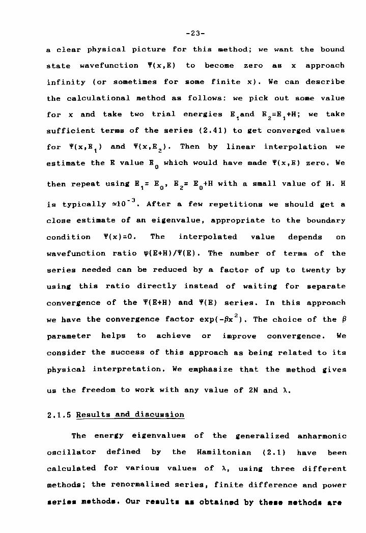
a clear physical picture for this method; we want the bound
state wavefunction ~(x,E) to become zero as x approach
infinity (or sometimes for some finite x). We can describe
the calculational method as follows: we pick out some value
for x and take two trial energies E1and E2
;;E 1+Hj we take
sufficient terms of the series (2.41) to get converged values
for ~(x,E1) and 'I'(x,E2). Then by linear interpolation we
estimate the E value Eo which would have made ~(x,E) zero. We
then repeat using E1;; Eo' E2
;; Eo+H with a small value of H. H
is typically ~10-3. After a few repetitions we should get a
close estimate of an eigenvalue, appropriate to the boundary
condition 'I'(x);;O. The interpolated value depends on
wavefunction ratio 1P(E+H)/'I'(E). The number of terms of the
series needed can be reduced by a factor of up to twenty by
using this ratio directly instead of wai ting for separate
converaence of the 'I'(E+H) and 'I'(E) series. In this approach
we have the converaence factor exp(-~x2). The choice of the ~
parameter helps to achieve or improve convergence. We
consider the success of this approach as being related to its
physical interpretation. We emphasize that the method gives
us the freedom to work with any value of 2N and X.
2.1.5 Results and discussion
The energy eigenvalues of the generalized anharmonic
oscillator defined by the Hamiltonian (2.1) have been
calculated for various values of ~, using three different
methods; the renormalised series, finite difference and power
.erie. method •• Our re.ult. a. obtained by the •• m.thod. are
-24-
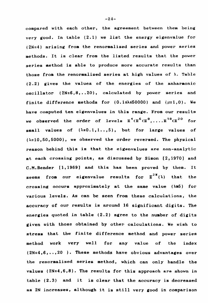
compared wi th each other, the agreement between them being
very good. In table (2.1) we list the energy eigenvalue for
(2N=4) arising from the renormalised series and power series
methods. It is clear from the listed results that the power
series method is able to produce more accurate results than
those from the renormalised series at high values of X. Table
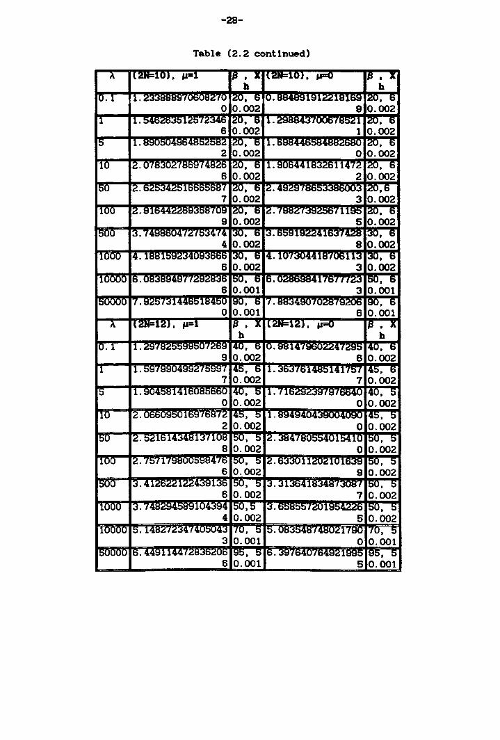
(2.2) gives the values of the energies of the anharmonic
oscillator (2N=6,8, •• 20), calculated by power series and
fini te difference methods for (0. 1~X~50000) and (#.1= 1,0). We
have computed ten eigenvalues in this range. From our results
we observed the order of levels R~<R6<Re, ••.. R1e<R2o for
small values of (X=0.1,1 •• ,5), but for large values of
(X=10,50,5000), we observed the order reversed. The physical
reason behind this is that the eigenvalues are non-analytic
at each crossing points, as discussed by Simon [2,1970] and
C.M.Bender [1,1969] and this has been proved by them. It
seems from our eigenvalue results for E2N(X) that the
crossing occurs approximately at the same value (XIiII5) for
various levels. As can be seen from these calculations, the
accuracy of our results is around 16 significant digits. The
energies quoted in table (2.2) agree to the number of digits
given with those obtained by other calculations. We wish to
stress that the fini te difference method and power series
method work very well for any value of the index
(2N=4,6, •• ,20 ). These methods have obvious advantages over
the renormalised series method, which can only handle the
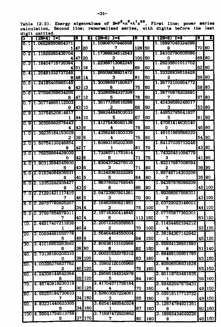
values (2N=4,6,8). The results for this approach are shown in
table (2.3) and it is clear that the accuracy is decreased
as 2N increases, although it is still very good in comparison
-25-
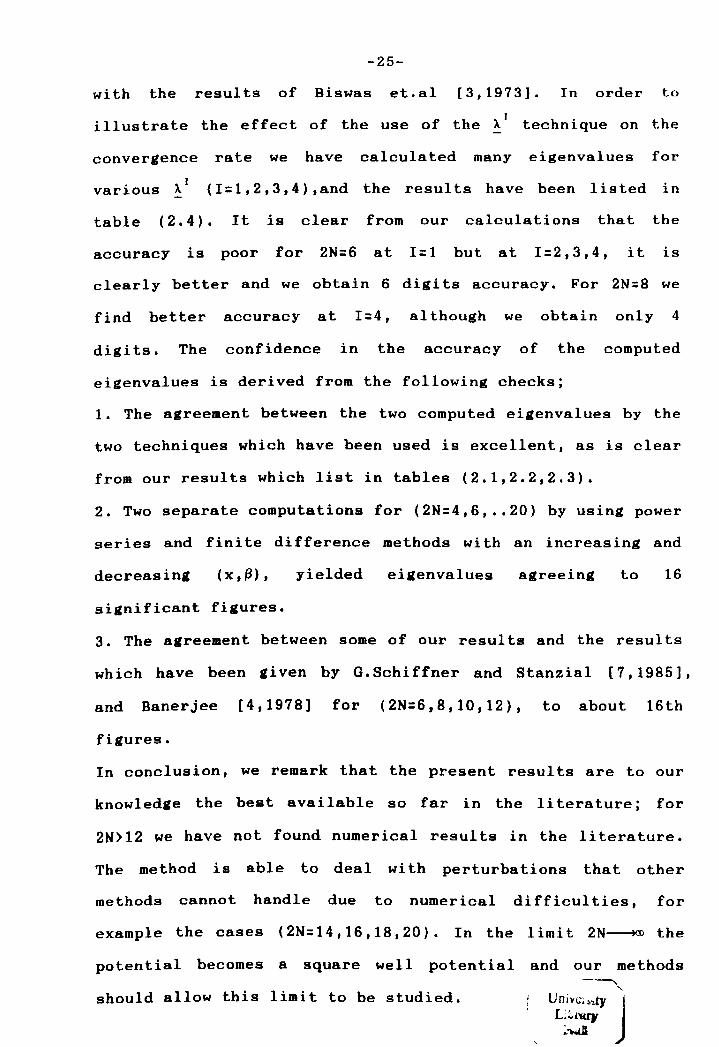
with the results of Biswas et.al [3,1973). In order to
illustrate the effect of the use of the Xl technique on the
convergence rate we have calculated many eigenvalues for
. , I var10US I\. (I=l,2,3,4),and the results have been listed in
table (2.4). It is clear from our calculations that the
accuracy is poor for 2N=6 at 1=1 but at 1=2,3,4, it is
clearly better and we obtain 6 digits accuracy. For 2N=8 we
find better accuracy at 1=4, although we obtain only 4
digits. The confidence in the accuracy of the computed
eigenvalues is derived from the following checks;
1. The agreement between the two computed eigenvalues by the
two techniques which have been used is excellent, as is clear
from our results which list in tables (2.1,2.2,2.3).
2. Two separate computations for (2N=4,6, •. 20) by using power
series and finite difference methods with an increasing and
decreasing (x,I3), yielded eigenvalues agreeing to 16
significant figures.
3. The agreement between some of our results and the results
which have been given by G. Schi ffner and Stanzial [7, 1985] ,
and Banerjee [4,1978] for (2N:6,8,10,12), to about 16th
figures.
In conclusion, we remark that the present results are to our
knowledge the best available so far in the li terature; for
2N>12 we have not found numerical results in the literature.
The method is able to deal wi th perturbations that other
methods cannot handle due to numerical difficulties, for
example the cases (2N=14,16,18,20). In the limit 2N~ the
potential becomes a square well potential and our methods
should allow this limit to be studied.
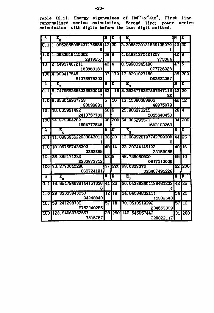
-26-
Table (2.1). Energy elgenvalues of H-p2+x2+~'. First line renormallsed series calculation. Second line; power series calculation. with digits before the last digit omitted.
A- Eo It ~ 1;1 lit &
0.1 [l. ~7176888 ;47 20 13 • .NOD 1,\J1315Z8135070 IIlZ ZO 8 1
1.0 11. ;1641530Z i3S its 14. 64881Z-(01lZIZU1 IIlZ 8 2918557 775364
.10. IZ.44817407Z11 140 ,4 18 • "<I4S4RO 4-( ,0 183869183 071126028
1100 14. 888411:;)4:;) 137 1170 17. 83019Z7159 36 !ZOO 51315818293 952522387
A- E2 IN 1& 1:3 It 1&
10 . 1 I:;). -(4P~' 14!'> 142 18 8 . .sO.GO I ns.Go I DO I 0".7116 42 IZO 7 22
11. 0 8.55504990-'-(:;)8 5 110 13. I! 142 1Z 93096881 49815079
110. 16.o.s0:sG1492 50 6 ,25. Duo~ID~15 IZ8 14 2413157183 5055640450
100 34. 8T~!oIW4?~? 36 200 54. 11:;)-(1 134 ZOO 1994177546 1603103269
A- !;, N K E5 lit K
0.1 11. ~~ 14-~qll ,38 ZO 113• i1877~1 44 25 1 0
1.0 18. 05-/001 l~~~n~ 149 :14 IZ;j. Z8-(4414tilZZ 48 1
16 3252895 23189085
10. 135.885171222 158 18 146 • I 158 10 2253873112 0817113006
:100 75. Df I 14n?R~ 137 IZZO 99. : f;j IZZ 12uU 669124181 315401491228
A- Ea lit 1& 1;7 lit IK
10.1 16.8:;)4-, ;144151336 41 Z5 zo.n4 ,188461232 42 25 6 4
11.0 12ts . H 12 18 134. ~4nR4R~~111 54 120 04248840 11332543
110 . 58.241~~D/.:J~ !:ff 18 IU.3510518382 157 10 9153240285 234653309
1100 123. ts41. '/O~OOI 38 250 1149. ;1443 131 1280 7816767 328822111
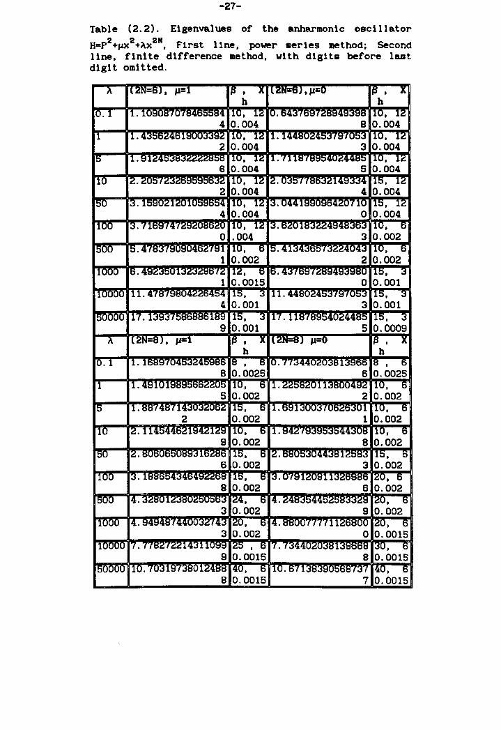
-27-
Table (2.2). Elgenvalues of the anharmonlc osclllator
H=p2+f.tX2+>.x2N
, First llne, power serles method; Second llne, finl te dlfference method, wl th digits before last dlgl t oml t ted.
, , 8 0.0015 7 0.0015
-28-
Table (2.2 continued)
• • 6 0.001 5 0.001
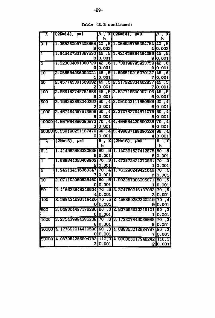
-29-
Table (2.2 continued)
• • 3 0.001 2 0.001
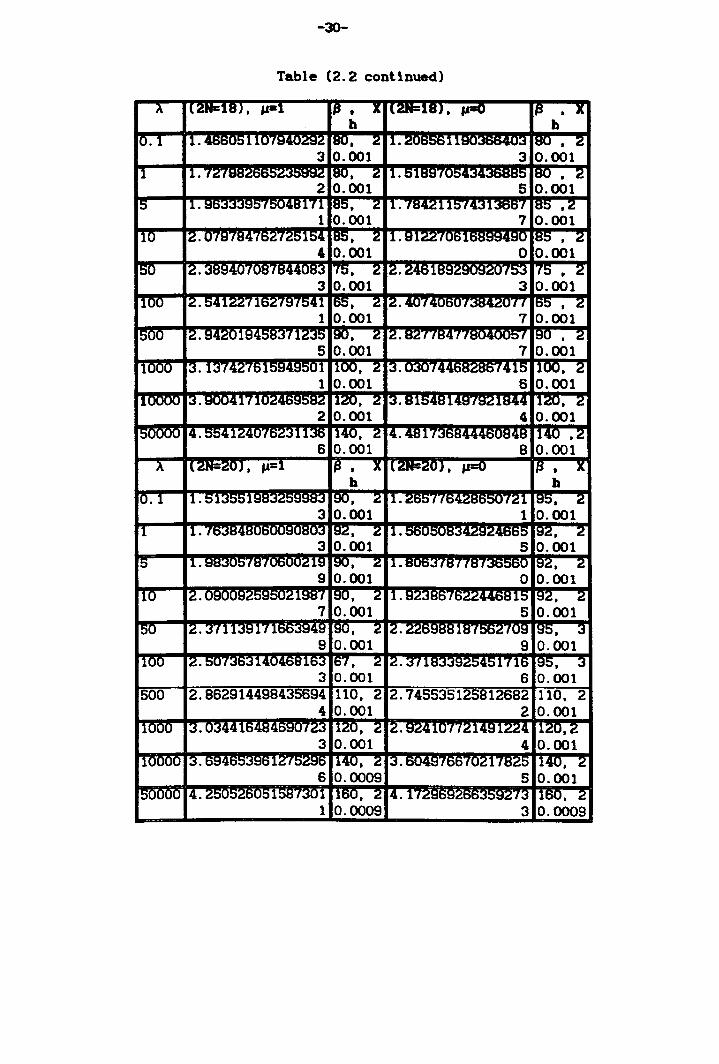
-30-
Table (2.2 continued)
• 1 0.0009 3 0.0009
-31-
Table (2.3). Energy elgenvalues of" H-p2+x2
+AI x2K • First Une; power .erles calculation. Second Une; renor.aUsed .erl... wl th digits before the last
1 ltt d dig t om e . lA (2H=4J I-I IN I: (2N=6) 1-4 IN le: \2H==---sJ ,at IN &
10 . 1 1. :ll~71 11. lUWtS/UI 11.lt)tstH LJ:;":I7.11.J:;QA
1 47 20 7 128 50 9 70 80
10.2 1. 11R~! i104 11. 1'1 1.as;'j12543 11. 241u"l 4 47 20 3 100 50 0 68 80
[0.3 1. 164047101 1.11. 11. ~..sotS (1 L"::;: It. 11011702 4 51 18 1 89 50 3 62 80
10.4 , 1. Z0481 u;"c; ,;,,/249 ,1. :147Z 11. 1.,19428 9 48 14 3 81 50 2 59 80
10 • 5 11. Z41 Rool4 i149 11. l(l~o"l 11. 30T,21 00954772 4 43 13 6 75 50 7 58 80
10 . 6 11.C;1 Ill7"::;:"::;: 11. '/~tI rt. ;j'dffU"df fl 5 47 12 5 78 50 7 57 80
10 • 7 11.30-,-'4865112003 11. 36 nf"::I'd::i 15Z88 rr.~ .... 8'117 0 43 10 2 66 50 3 53 80
10 . 8 11. 3375ll ... ..,()~I4817 11. "lRR7J1 A CA· [l.n :1~5Dn937
1 44 10 5 67 50 5 61 90
10.9 11. 30! i78443 11. 4127".11. ~138 rr. 4706I4~I40 4 43 9 4 78 60 0 46 80
11. 0 1. :i~"":i!i164153029 11. .II.~HR~4F;l!-lnr :'c:-I!-I 1.49101 2 39 8 4 76 60 1 54 80
12.0 1. 60154 , ~r I~.II.RRH.II. 11. 11: !l.l)U3-'U;j::;~
8 42 7 1 81 70 1 43 80 3.0 1. -'O'd! 1. I;"c;t50/11751614 [l.~S:;1094779·
0 42 6 5 71 75 3 41 80 4.0 I.S031 LH~nn 1. R"lnll'I;j4;jf::;UIO 1. 8221'7Slff
5 43 6 3 71 80 2 39 80 0.0 2.01834004 :1 .1. S' 7ll' .... : 1. 8874871.11.'";1n'";17nR
6 40 5 5 64 80 7 35 80 6.0 Z. ..,n ... ~~~~~~~4~7 11. 'd"d;j I "dUO" I T.~('d-" 7nQ
9 43 5 8 66 80 3 45 100
7.0 Z.Z129142I1174I5 12.04·Ic;;j'duloU1261 1. QQ7QRI 1-,::;ti~3ul
7 46 5 3 70 90 2 43 100
18.0 12. C;tI ( 0 ( ( I1 12. 1n.a ~1951 [G. U3f nABOOl 2 34 4 2 75 100 7 44 100
19 . 0 I Z . ;j lO'd (8549783 11 12. 157tR":Inn414840 12. U.,-,::;t:i~.,r~~7~111 7 40 4 6 113 150 7 53 120
110. 12. 44~17407211838 12. "uo I rz.TI4H.II..II.R~194212
1 40 4 2 70 100 4 52 120 [ZO. 13. nn~~44~1t:it:it:i.,.(~ 12. nn04 12.38184367142942
5 49 4 4 94 150 1 45 120
~O. 13.4IOIRW \R~ IZ. 1113In7~RR 12. 5~38S9l5BS 6 38 80 8 82 150 8 51 140
140. i3. -'~139' 110 13. 000315320'/o~12 12. R~.II.R~105951785 0 39 100 1 83 160 4 53 150
150. :4. 1?"ID"d" I lOC; 13. 15902120' 12. 1'dJI828
2 40 120 2 76 160 6 55 150
~O. i 4. 243()~ Ill11Rll~R4 13. .1~4~~4R78 [Z.mrIT97S:J(9I835 6 29 120 5 84 180 1 56 160
[70. 14. 4574UI:P~Zi I:HS 13 .41704571758164 12. ~A.II.R"''''!of(019431 2 30 125 4 70 160 4 49 150
[BD. 14. RH7HtiI84·pCIJ ... :u 13. H7Rf 1/ '4n~1 13.05918117713722 7 34 150 3 65 160 9 49 150
[90. 14. 83Z3 44·,Jt'i .... :·uu~ 13.62541 1~?4 13.1207U84921351 6 34 160 1 67 160 6 SO 160
100 14.99941754513758 13. 716S747.~C ·.mRR~ 13~":I1r~.II.Q?7R . ... ............ 5 37 170 7 80 180 8 46 150

-32-
Table (2.4). Energy of ground state levels, by using renormal1sed series method at A-1, The number in the bracket correspond to exact value.
-33-
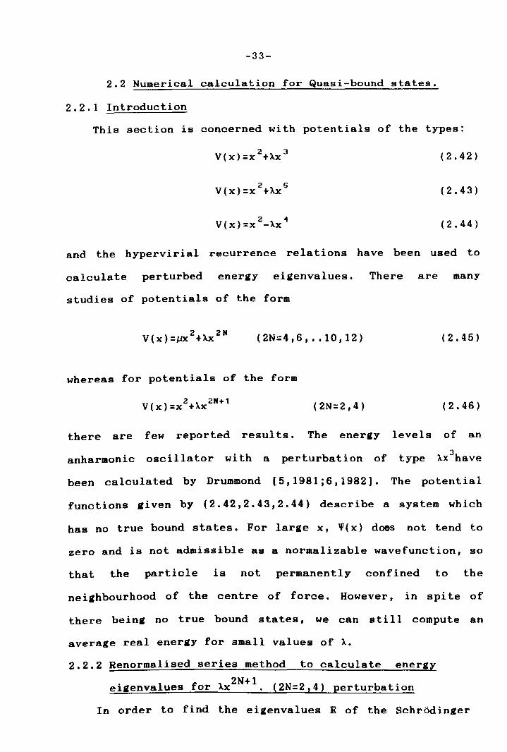
2.2 Numerical calculation for Quasi-bound states.
2.2.1 Introduction
This section is concerned with potentials of the types:
2 3 V(x)=x +Xx
2 5 V(x) =x +Xx
2 4 V(x)=x -Xx
(2.42)
(2.43)
(2.44)
and the hypervirial recurrence relations have been used to
calculate perturbed ener~y eigenvalues. There are many
studies of potentials of the form
(2N=4,6, •. 10,12) (2.45)
whereas for potentials of the form
(2N=2,4) (2.46)
there are few reported results. The energy levels of an
anharmonic oscillator wi th a perturbation of type 3 Xx have
been calculated by Drummond [5,1981 ;6, 1982]. The potential
functions ~iven by (2.42,2.43,2.44) describe a system which
has no true bound states. For large x, If/( x) does not tend to
zero and is not admissible as a normalizable wavefunction, so
that the particle is not permanently confined to the
neighbourhood of the centre of force. However, in spi te of
there bein~ no true bound states, we can still compute an
average real energy for small values of X.
2.2.2 Renormalised series method to calculate energy
ei~envalues for Ax2N+l. (2N=2,4) perturbation
In order to find the eigenvalues E of the Schrodinger
-34-
equation:
[ d2 2 2H+1] - + x +Xx '(x)=E'(x) dx 2
(2N=2,4) (2.47 )
We shall use the hypervirial relations (2.3) in calculating
the perturbation energy series. Drummond's approach is based
on a method due to Bender and Wu [1,19691. It uses recurrence
relations to calculate the perturbed energy and wave
function. We should point out that Drummond used extrapolated
values based on the first few terms of the energy series, but
in our approach we calculate many terms of the series. Also
in our approach we tried out Aitken's transformation in order
to increase the accuracy, but unfortunately it did not seem
to help to improve the accuracy of our resul ts for this
problem. In order to improve the convergence properties of
the perturbation series we used a rearrangement of terms in
the potential (renormalised perturbation series).
To illustrate this technique we can rewrite the
potential (2.46) as follows
V(X)=~2+A(X2H+1_KX2)
where
J.l= l+XK
(2.48)
(2.49)
The new perturbation series is still divergent but its
di vergence begins for hiath values of A, so that for low
values of X we findagood energy value. Inserting the series
expansions given by equations (2.6) and (2.7) into (2.3) and
taking into account the potentials coefficients
(2.50)
-35-
V =A.. 2N+1 t
(N= 1,2 ) ( 2 • 51)
we obtain the recurrence relations
(2N+2)~ E(J)A(N,M-J): (2N .. Lt) [I1A(N+2,M)-KA(N+2,M-l)]
+ [2N+2n+3]A(N+2n+1,M-1)- ~[N2-1]A(N-2,M) (n=1,2) (2.52)
Applying the Hellmann-Feynman theorem as given by equation
(2.14), we obtain a recurrence relation in the form
(M+l)E(M+l):A(2n+l,M)-KA(2,M) (n=1,2) (2.53)
It is clear now that from equations (2.52) and (2.53) we
obtain the full set of A and E coefficients starting from the
unperturbed energy
E(O)= (2n+1)~11 (2.54)
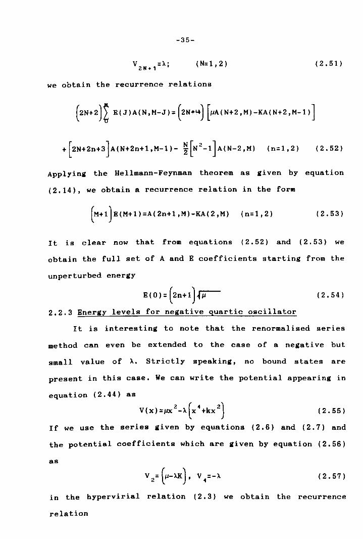
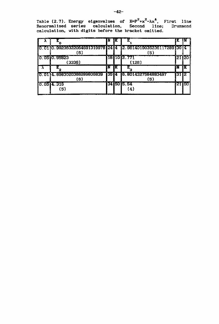
2.2.3 Energy levels for negative quartic oscillator
It is interesting to note that the renormalised series
method can even be extended to the case of a negative but
small value of A.. Strictly speaking, no bound states are
present in this case. We can write the potential appearing in
equation (2.44) as
2 (.. 2) V(x)=11X -A. x +kx (2.55)
If we use the series given by equations (2.6) and (2.7) and
the potential coefficients which are given by equation (2.56)
as
(2.57)
in the hypervirial relation (2.3) we obtain the recurrence
relation
-36-
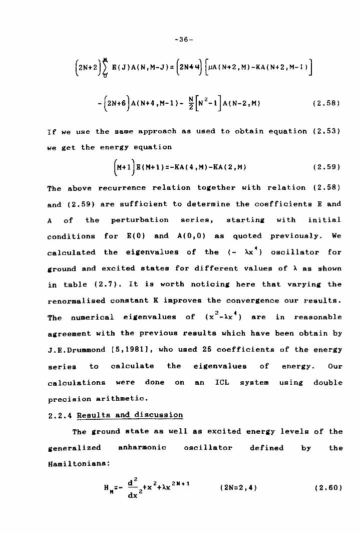
( 2 N + 2 ) ~ E ( J ) A ( N , M - J ) = (2 N t4- 4) [/lA ( N + 2 , M ) - KA ( N + 2 , M - 1 ) ]
(2.58)
If we use the same approach as used to obtain equation (2.53)
we get the energy equation
(M+1)E(M+1)=-KA(4,M)-KA(2,M) (2.59)
The above recurrence relation together with relation (2.58)
and (2.59) are sufficient to determine the coefficients E and
A of the perturbation series, startin& with initial
conditions for E(O) and A(O,O) as quoted previously. We
calculated the ei.cenvalues of the (- AX 4) oscillator for
ground and excited states for different values of A as shown
in table (2.7). It is worth noticing here that varying the
renormalised constant K improves the convergence our results.
The numerical eigenvalues of (x2_"-x4) are in reasonable
agreement with the previous results which have been obtain by
J.E.Drummond [5,1981], who used 25 coefficients of the energy
series to calculate the eigenvalues of energy. Our
calculations were done on an leL system using double
precision arithmetic.
2.2.4 Results and discussion
The ground state as well as excited energy levels of the
generalized anharmonic oscillator defined by the
Hamiltonians:
(2N=2,4) (2.60)
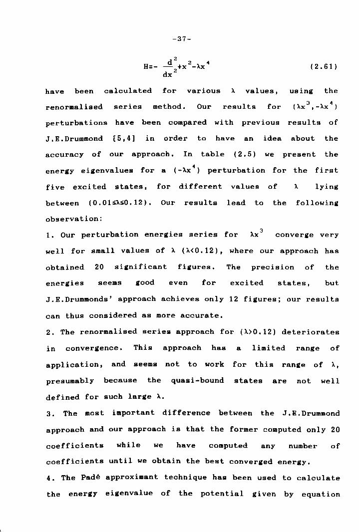
-37-
d 2 2 4 H=- - +X -XX
dx2
( 2 .61 )
have been calculated for various X values, using the
renormalised series method. Our results for 3 4 (XX ,-Xx)
perturbations have been compared with previous results of
J.E.Drummond [5,4] in order to have an idea about the
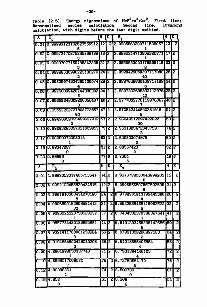
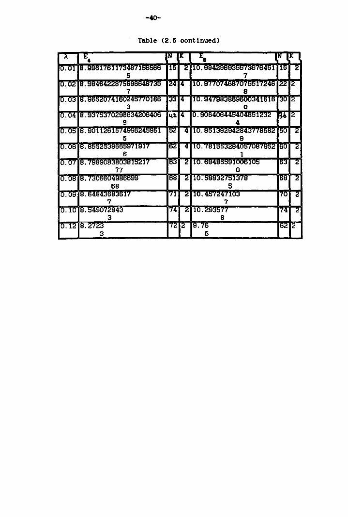
accuracy of our approach. In table (2.5) we present the
energy eigenva1ues for a 4 (-Xx ) perturbation for the
five excited states, for different values of
first
lying
between (0.01sXsO.12). Our results lead to the following
observation:
1. Our perturbation energies series for converge very
well for small values of >.. (>"(0.12), where our approach has
obtained 20 significant figures. The precision of the
energies seems good even for excited states, but
J.E.Drummonds' approach achieves only 12 figures; our results
can thus considered as more accurate.
2. The renormalised series approach for (X>0.12) deteriorates
in convergence. This approach has a limited range of
application, and seems not to work for this range of X,
presumably because the quasi-bound states are not well
defined for such large X.
3. The most important difference between the J.E.Drummond
approach and our approach is that the former computed only 20
coefficients while we have computed any number of
coefficients until we obtain the best converged energy.
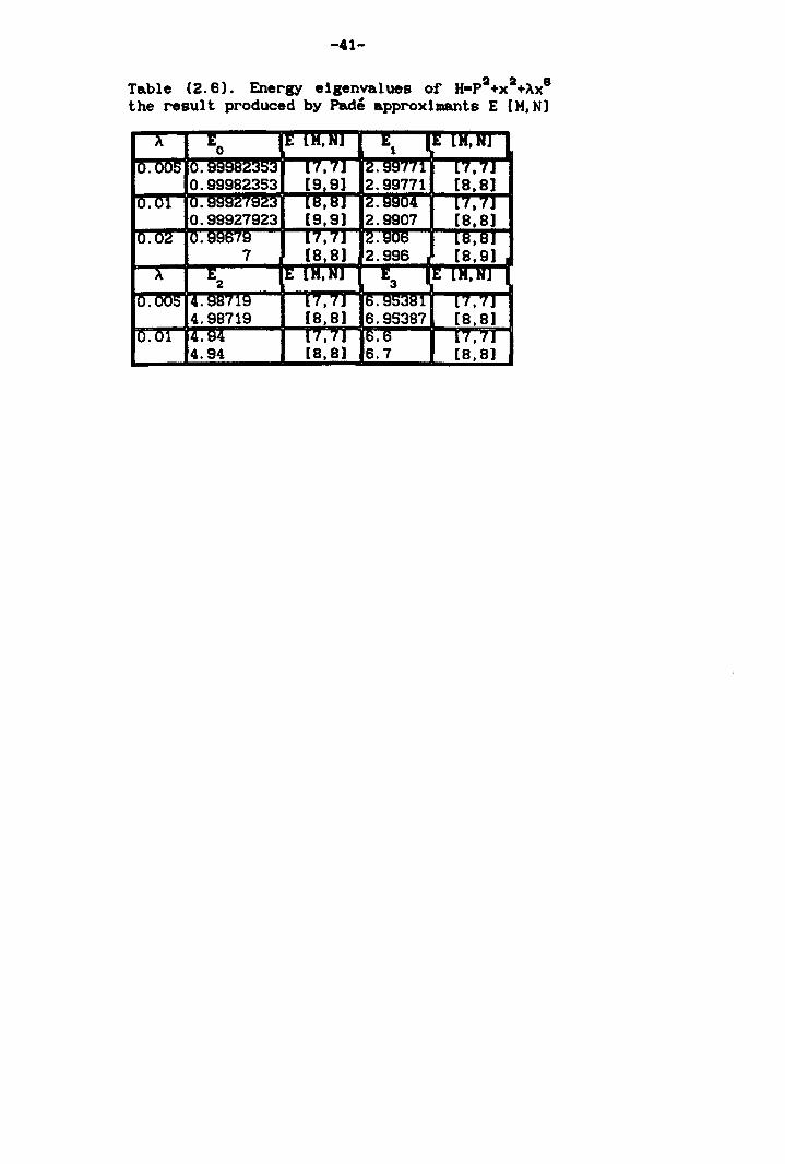
4. The Pade approximant technique has been used to calculate
the energy eigenvalue of the potential given by equation

-38-
(2.43) for low values of X, because the energy series is more
speedily divergent than that for the potential (2.42). Our
results in table (2.6) exhibit this behaviour. This technique
is reviewed in more detail in chapter 4. In the absence of
other reported results (to the best of our Knowledge), we
have calculated each eigenvalue for two values of [M,N) in
order to estimate the accuracy of our results.
-39-
Table (2.5). EnerlY elgenvalues of H-p2+XI
+).x3. First llne; Renormallsed series calculation. Second line; Drummond calculation. with digits before the last digit omitted.
A Eo N IK E1 I IN I lIe I 0.01 o. r1231R7~' IlZ 11Z 2 IZ. 1f11~~~ 1r;,7 T3- --z
6 1 0.02 O. t:Jl:n:H ,(UtS( 1188 116 ~ I~. HHH"';"!1471 111 i17 12
3 1 0.03 O. t:J~~~f~111! 'A-7~~R !21 Z IZ • : l'rotjl::III::) 116 '22 2 . _-
5 8 -0.04 O. 1136279 124 Z Z.QQ?R4 I( (17080 126 ,2
2 40 ,0.05 O. I [~rl4~Q"106074 129 Z Z.tlOOI "11189 ~ rz
4 6 '0.06 0.t:J~1 ·?~7!1/l1 134 2 2. 98:S1 1113876 138 [2-
8 40
10.07 10. ,J7 140 IZ IZ. 'd"fU~~TftH 199'(UUtH ~ rz 3 7
[0.08 10. :u. (908772567 147 IZ IZ. 97n~1l 11916 [Sl rz 80 9
10.09 Iu.ac ftH2 157 12 2. C~~I/l 11:;j122974 [58 [2 0 30
10.10 '0.QQ7! "l~'T63 I ~na~53 75 IZ Z.9531965472043759 74 12 1 3
10.12 10. tl "lCW"U3 183 IZ 2. 114978 180 12 1 2
10.15 10. 98347687 ~3 12 12. 88!:>tf{423 gz rz 9 2
10.ZO 10. T{ 18 12. 'T564 48 6 3 5
A E2 N ~ E3 N X
0.01 4.9988053317405753541 14 2 6.9976788050043899205 15 2 4 0
[0.02 14. 995Z' 1~1I.~RR~Q4~4RI5 i 19 Z 16. ~~UbtsoootS 1 tSO IRQ7~QR 121 12
9 8 10.03 14. 989181 'l~'l/l'l/l~781B6 1~4 ~ 16. 97B93018131CCIIl/l~"lD~ 126 2
5 4 [0.04 14. r1528 ,1Z 131 2 16 . 1/l~'ll1 [33 2
30 9 [0.05 14. ['l~rr{ccc:)RQ' :7 :37 Z 16.Q414 ,I 1/541 141 2
1 1
10.06 14. 955TrM4R(l1R7~R7~ql 144 2 16 • 9131 ?Q~4RR~Qq14~~RR ISO 2 0 9
10.07 14. 939141ntststsU' .............. 106 Z 16.87991:41 11580 164 2 9 3
10.08 14.91: Rr174~' , ... ~98 i68 ~ It). 8401~ __ ... __ J5584 68 2 3 4
10.09 14. :-,{40 n ~ 16. "{931 ;125 72 2 1 4
0.10 14.869901'1 75 Z 6.1..s10..sbb417Z 76 --z 7 6
0.12 4. RI ~RR16-1 74 2 6.093703 81 2 4 0
0.15 4.658 151 2 6.Z08 ~ --z 8 8
-40-
Table (2.5 continued)
3 6
-41-
Table (2.5). Energy elgenvalues of H_p2+x2+AXS
the result produced by Pade approxlmants E [H,N]
, , 4.94 [8,8) 6.7 [8,8)
-42-
Table (2.7). Energy eigenvalues of H=p2+x2_~x~, First line Renormalised series calculation, Second linej Drummond calculation, with digits before the bracket omitted.
(3336)
(5) (4)
-43-
2.3 Energy levels of double-well anharmonic oscillator
2.3.1 Introduction
The aim of this section is to investigate numerically the
eigenvalues of double-well potentials with form given as
below:
Z2 X 2 + x2" V(x)=- (2N=4,6,8, ...... 28, 30) (2.62)
The most studied system of this kind is the quartic
double-well potential (2N=4). The calculation of eigenvalues
for the Schrodinger equation wi th double-well potential has
received great attention from us. We extended our
calculations to higher powers (2N=4,6,8 ..... 28,30), since our
methods free our hands to compute the eiatenvalues for such
hiather values of 2N. The treatment of the double-well
potential (2N=4) has attracted many authors. For instance,
R.Balsa et. al [17,1983] have computed the energy
eigenvalues for 2N=4,(OSZ2~100) and 0~n~21; their results
produce 12 digits accuracy. R.M.Quick and H.G.Miller
[18,1984] have computed for 2N=4, Z2=50 and (0~n~79); they
used a non-perturbative method involving matrix
diagonalization to calculate some energy levels. Our
approaches will use a perturbative method as well as a
non-perturbative method. Our main object is to demonstrate
that both approaches work and are able to produce excellent
2 accuracy in spite of high values of Z , 2N and state number
n. It is important to point out that some of our results for
this problem are not available in the literature, so the
values which are listed in our tables have been checked at
least by two methods. The aatreement in our calculated results
-44-
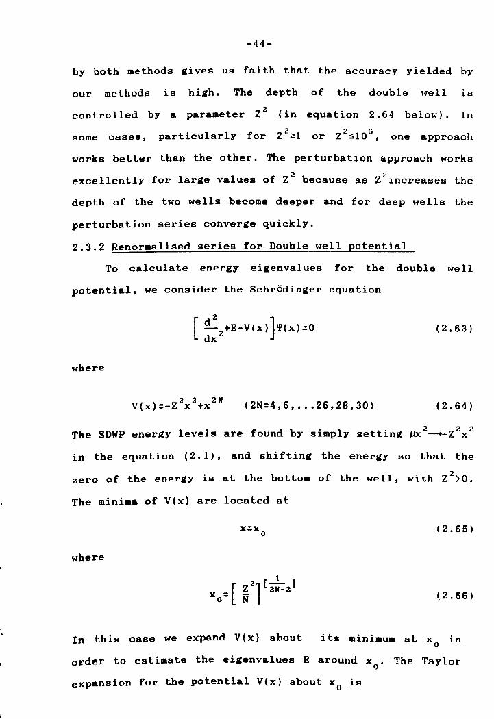
by both methods gives us faith that the accuracy yielded by
our methods is high. The depth of the double well is
2 controlled by a parameter Z (in equation 2.64 below). In
some cases, particularly for Z2~1 2 6 or Z ~1 0 , one approach
works better than the other. The perturbation approach works
excellently for large values of Z2 because as Z2increases the
depth of the two wells become deeper and for deep wells the
perturbation series converge quickly.
2.3.2 Renormalised series for Double well potential
To calculate energy eigenvalues for the double well
potential, we consider the Schrodinger equation
where
2 2 2N V(x):-Z x +x (2N:4,6, ••• 26,28,30)
(2.63)
(2.64)
The SDWP energy levels are found by simply setting ~x2~_Z2x2
in the equation (2.1), and shifting the energy so that the
zero of the energy is at the bottom of the well, with Z2>O.
The minima of V(x) are located at
(2.65)
where
(2.66)
In this case we expand V(x) about its minimum at Xo in
order to estimate the eigenvalues B around x . The Taylor o expansion for the potential V(x) about x is o
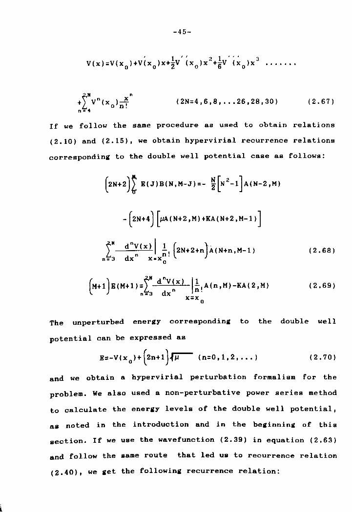
-45-
!N n
n X + V (XO)nr n=4
(2N:4,6,8, ••• 26,28,30) (2.67 )
If we follow the same procedure as used to obtain relations
(2.10) and (2.15), we obtain hypervirial recurrence relations
corresponding to the double well potential case as follows:
- (2N+4) [1lA(N+2 ,M) +KA(N+2 ,M-l)]
~N dnV(X)I!, (2N+2+n)A(N+n,M-l) L d n n. n=3 X x-x o
(2.68)
(2.69)
The unperturbed energy corresponding to the double well
potential can be expressed as
B=-V(x o )+ (2n+1 )~J.l ( n= 0, 1 , 2 , ••• ) (2.70)
and we obtain a hypervirial perturbation formalism for the
problem. We also used a non-perturbative power series method
to calculate the energy levels of the double well potential,
as noted in the introduction and in the beginning of this
section. If we use the wavefunction (2.39) in equation (2.63)
and follow the same route that led us to recurrence relation
(2.40), we get the following recurrence relation:
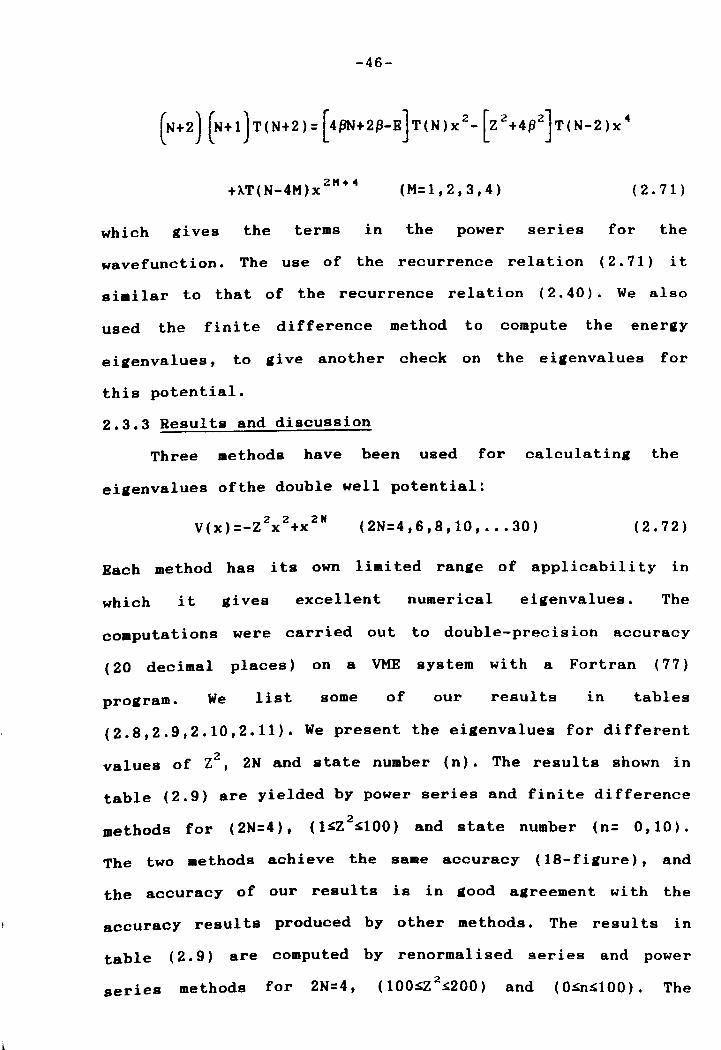
-46-
+AT(N_4M)x 2M+
4 (M=1,2,3,4) ( 2 . 71)
which gives the terms in the power series for the
wavefunction. The use of the recurrence relation (2.71) it
similar to that of the recurrence relation (2.40). We also
used the finite difference method to compute the eneriY
eiaenvalues, to ai ve another check on the eiaenvalues for
this potential.
2.3.3 Results and discussion
Three methods have been used for calculatina the
eiaenvalues of the double well potential:
2 2 2N V(x)=-Z X +x (2N=4,6,8,10, ..• 30) (2.72)
Bach method has its own limited ranae of applicability in
which it gives excellent numerical eigenvalues. The
computations were carried out to double-precision accuracy
(20 decimal places) on a VME system with a Fortran (77)
proaram . We list some of our results in tables
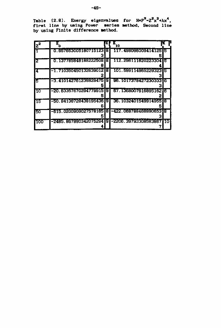
(2.8,2.9,2.10,2.11). We present the eiaenvalues for different
2 values of Z , 2N and state number (n). The results shown in
table (2.9) are yielded by power series and finite difference
methods for (2N=4), (1~2~100) and state number (n= 0,10).
The two methods achieve the saBle accuracy (18-fiaure), and
the accuracy of our results is in aood al(reement with the
accuracy results produced by other methods. The resul ts in
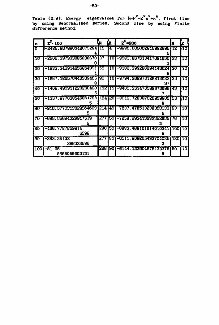
table (2.9) are cOBlputed by renormalised series and power
series methods for 2N=4, (100~Z2~200) and (O~n~100). The
-47-
agreement between the two methods is in general good to about
16-figures but at low Z2values (Z2=100) and high state number
(BO~n~100), the renormalised series faces difficulties in
producing the eigenvalues, while the power series method is
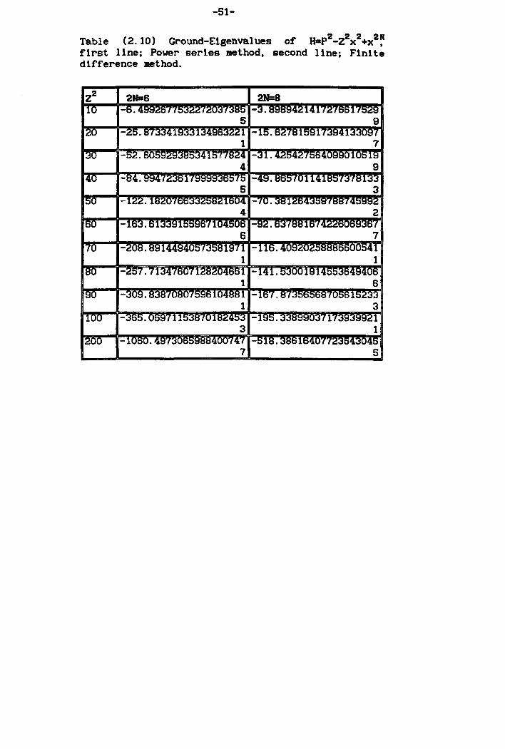
able to give very high accuracy. In table (2.10) we list
ground state results for (2N=6,8,10,12), and for 2N=6,B;
10~2~200, and for (2N=10, 12); (50~Z2~5000). The agreement
between results is very good (20-digi ts). In the present
work, we consider not only 2N=4, but extend the work to high
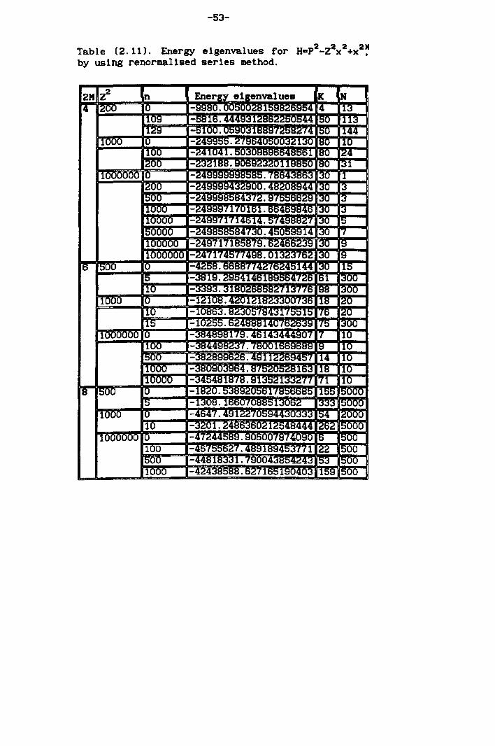
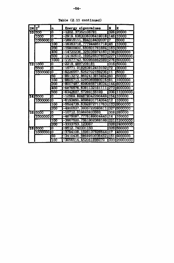
powers (2N=6,8, 10 •.• 28,30). We list in table (2.11) the
results for (2N=4,8,10,12, •.. 16,1B) and
(0~~106). It is clear from our results that the renormalised
series method achieves very hiah accuracy (20 diai ts). We
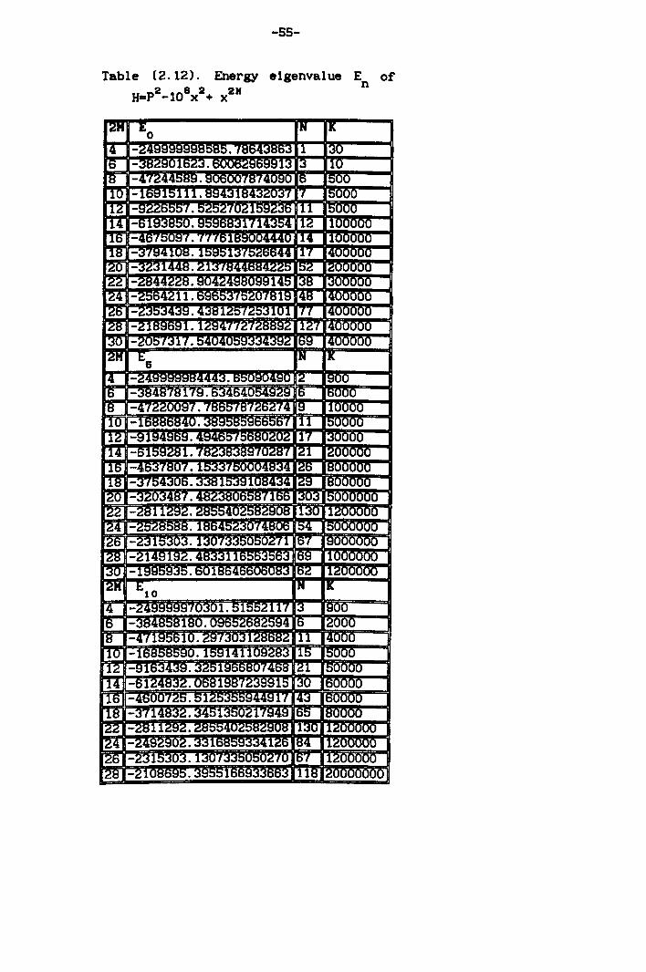
show in table (2.12) the results for (2N=4,6,8 ... 30);
z2=10 6and n=0,5,10. Our results for the double well potential
have the following consequences:
First the three methods all yielded excellent accuracy for
hiah values of Z2, 2N=4,6,B, •• 28,30 and state number n. The
renormalised series produce 20-diaits while the power series
and finite different method yield around 1B-digits.
Secondly the renormalised series work and converge very well
(even with zero renormalised constant k=O) for high values of
Z 2, but for low values of Z 2 the accuracy depends on the
choice of the constant K. On the other hand, there was seen
in some perturbation series calculations the phenomenon of
boaus convergence of the perturbation series. We can overcome
this situation by running the same series for different
values of the renormalisation constant K, or by using another
-48-
method to compute the eigenvalues.
Thirdly, as 2N increases the order of the series (M) must be
increased to get converged eigenvalues. For instance at
(2N=6, Z2= 10 6, n=100) the order of series M=9 suffices but
for 2N=16 with the same parameters as for 2N=6 the order
M=221 is needed. Therefore, the computation requires more
time to obtain a converged eigenvalue. The numerical
investigations of the double well potential shows the
applicability of the renormalised series method is limited to
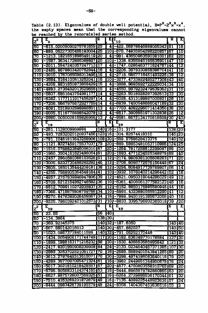
small values of Z2; this behaviour is clear from our results
in table (2.9). In conclusion, we remark that a large part of
our results (as noted in beginning of this section) are not
available so far in the literature for any value of 2N and A.
-49-
222 , Table (2.8). Energy elgenvalues for H-P -Z x +~x , first line by uslng Power serles .et bod , Second llne by using Finite difference .et hod.
4 7
-~-
Table (2.9). Energy eigenvalues for H=p2_Z2x2+x'. first line by using Renormalised series, Second line by using Finite difference method.
8568086503131 8
-51-
Table (2.10) Cround-Eigenvalues of H=p2_Z2x2+x2~ first line; Power series method, second line; Finite difference method.
7 5

-52-
Table (2.10 continued)
5 3
-53-
Table (2.11). Energy eigenvalues for H.p2_Z2x2+x2~ by using renormalised ser1es method.
-54-
Table (2.11 continued)
-55-
Table (2.12). Energy elgenvalue En of
H=p2_t08x2+ X2K
-$-
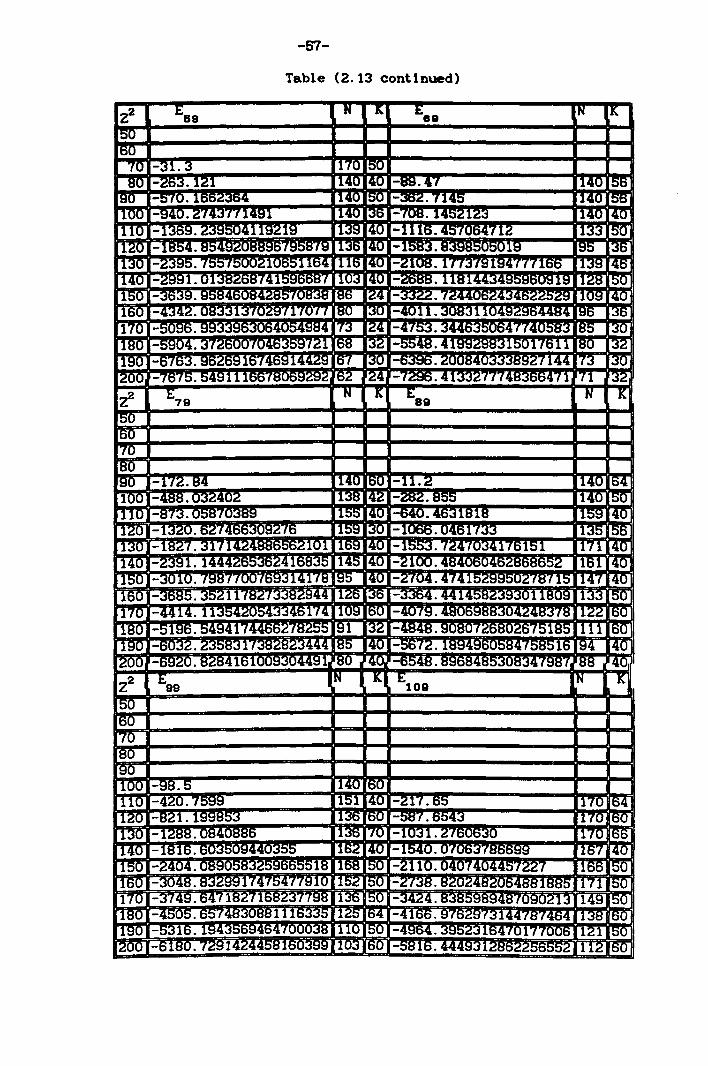
Table (2.13). Eigenvalues of double well potential. H_p2_Z2X2+X'. the empty spaces mean that the corresponding elgenvalues cannot be reached b the renormlsled serIes method.
-57-
Table (2.13 continued)

-58-
Table (2.13 continued)
-59-
2.4 Expectation value calculations <x 2N )
2.4 .1 Introduction
Our aim in this section to find expectation values <x 2N)
for the potential
(2.73)
However to find an expectation value such as <x 2N) for a
bound state, we need to have the ei.enfunction ~(x) for all
x if we wish to apply the definition
(2.74)
To find ~(x) for arbitrary x and for any state number
(n:O,1,2 .• 9,lO), is not easy. However Killin.beck [12,1979]
has applied a very simple perturbative numerical algori thm
for the calculation of an expectation value, based on the
formula
1 = Lte----+ 0 2£ [ 2N 2N ] E(H + EX )- E(H - EX ) (2.75)
This al.orithm demonstrate that expectation values can be
determined by an approach based on ei.envalue calculations,
without the explicit use of wavefunctions. The way in which
we can calculate is as follows; we do two calculations, to
.et two B values, with ~£X2N included in the potential
2N £x
(2.76)
(2.77)
where £ is a very s.all number. The value of <X2N
) is then
-60-
given by
(2.78)
The Hellmann-Feynman and the virial theorem also provide
relationships between the energy and the expectations values
<x 2 >, <x4> which take the form
[ ] H [ ] H+2 [ ] H+4 N[ 2 ] N-2 2E N+l <x >: 2N+4 <x >+ 2N+6 A<X >-2 N -1 <x > ( 2 . 79 )
We used the Hellmann-Feynman theorem to calculate the
expectation values along with the energies for potential
(2.73), and can calculate the coefficients in the series
'> n 2 3 <x~ >:A(2n,0)+A(2n,1)A+A(2n,2)A +A(2n,3)A + .. (n:l,2) (2.80)
234 E:E(O)+E(l)A +E(2)A +E(3)A +E(4)A......... (2.81)
2.4.2 Results and discussion
The energy eigenvalues and expectation values <XZN>
(2N:2,4) of the potential V(X):X2
+AX4
have been calculated
for state number 0~~10 and for various values of
(A:0.l,1,10,lOO) using three different methods; the
renormalised series method, the finite difference method and
the power series method. The energy and expectation values as
obtained by these methods are compared with each other, the
agreement between them being very good. To use power series
or f ini te di fference methods to calculate the expectation
values <~IX2NI'> (2N:2,4) of the x2", we simply calculate the
energy twice, once for Hamiltonian H+CX2N
and once for
-61-
2" h H-£x • According to t e first order energy formula the
difference between them equals if is
sufficiently small. It is important to point out the effect
of the parameter value £ in obtaining high accuracy of <x 2 ">. The best values of £ in this calculations have been obtained
by numerical search. An £ value -8 £=10 atave 15 digits
accuracy, but larger values such as £) 10 - 8 produced less
accuracy. Our results were checked by noting that the
independently calculated values of B, 2 .. <x ) and <x > obeyed
the virial theorem
2 .. B=2<x >+31<x > (2.83)
In tables (2.15) and (2.16) we list the energy E , E and the - +
expectation values for <x 2") (2N=2,4) for state number 0~n~10
and for -3
p.=0.1,1,10,100), with the value £=10 . This value
seems good for high values of 1 and gives 10 digits accuracy,
but the accuracy decrease with small values of X. The results
presented in tables (2.15,2.16) are computed by power series
and renormalised series methods. The agreement between them
is very good. In table (2.17) we present the energy
eigenvalues and the expectation values by using renormalisd
series and power series, -8 with the smaller value £=10 . The
two methods achieve the sa.e accuracy. We wish to mention
that to produce results by usinat renormalised series with a
high accuracy, we worked hard to achieve that, e.g by
changing the value of the overflow parameter (2", N=I,2,3 .. )
and also by increasing the dimension of B(N,M) together with
varying the renormalised constant. We checked some of our

-62-
results which are given in tables (2.16,2.17,2.18) by using
the finite difference method, which gives the same accuracy
as that achieved by the power series. Our results also agree
with those available results reported in the literature.
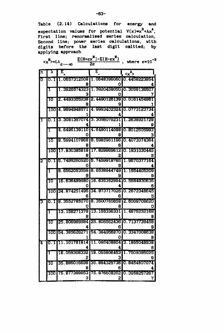
-63-
Table (2.14) Calculations for energy and
expectation values for potential V(X).x2+~x'. First line; renormalised series calculation. Second line; power series calculations. with digits before the last digit omitted; by applying approach
N E(H+cxN)-E(H-cxN) 3 <x-~=Lt • where c-10-
c~ 2c
3 2 7
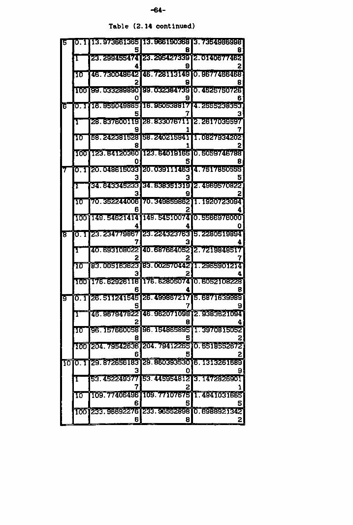
-64-
Table (2.14 continued)
6 8 2
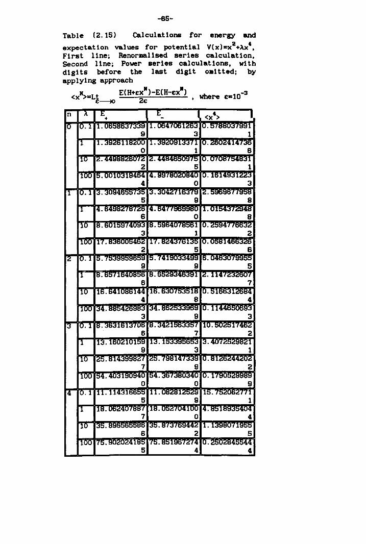
-85-
Table C2.15) Calculations for energy and
expectation values for potential V(x)=x2+).x',
First linei Renormalised series calculatlon. Second llne; Power series calculatlons, with digits before the last digit oaittedi by applying approach
ECH+&x")-ECH-£x·) -3 2& ' where £1:10
5 4 4
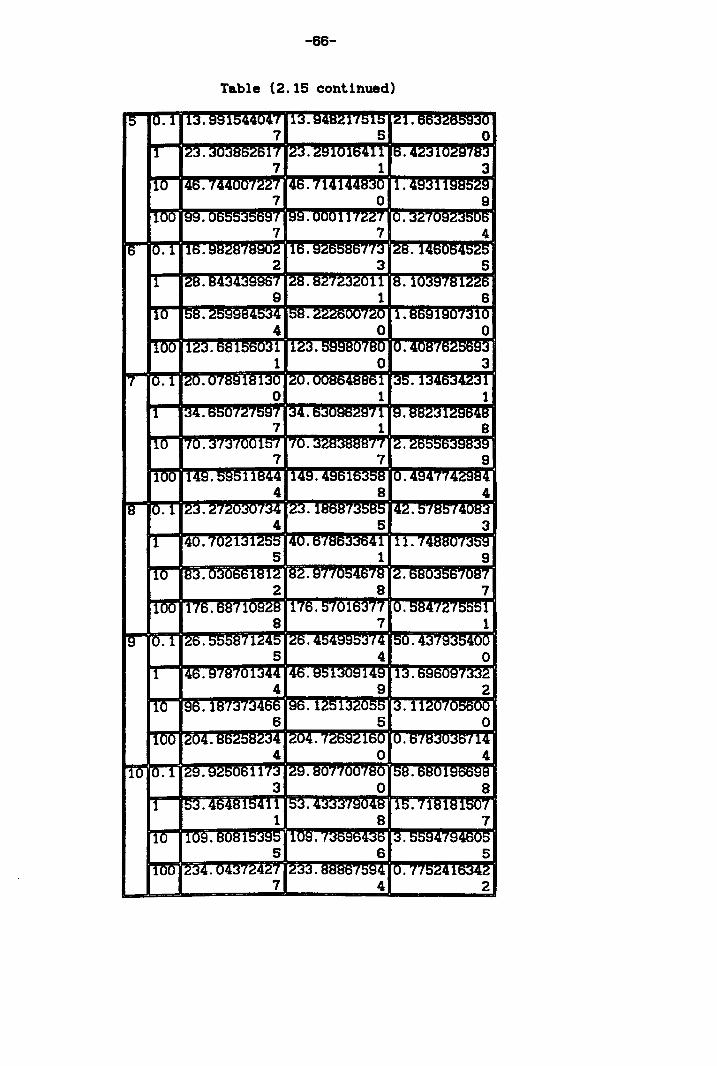
-66-
Table (2.15 contlnued)
7 4 2
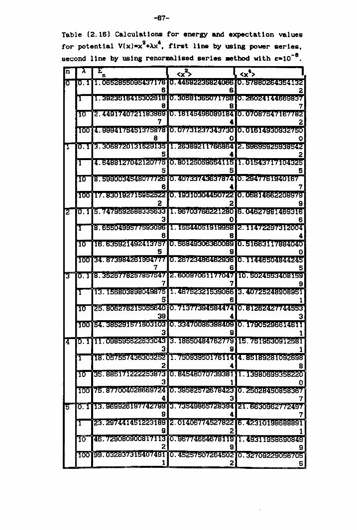
-67-
Table (2.16) Calculations for energy and expectation values 2 ,
for potential V(x)-x +i\x • first Une by using power series,
second line by using renormalised series .etbod with e_1C-B.
1 2 5
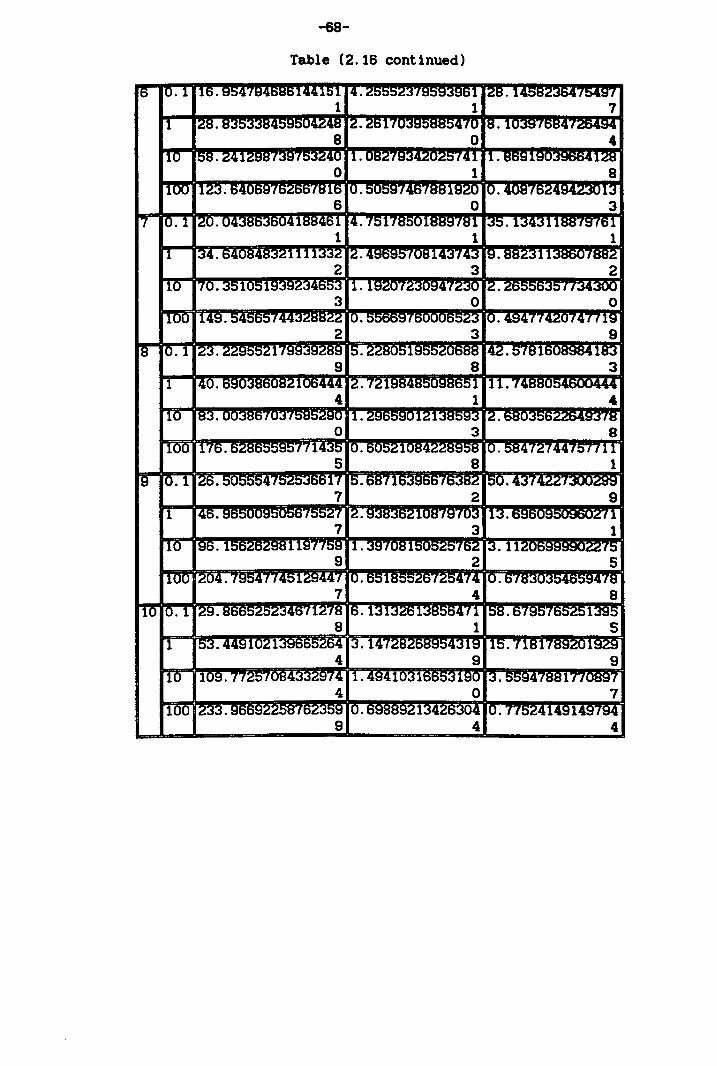
-88-
Table (2.16 continued)
9 4 4
-69-
CHAPTER THREE
TWO, THREE AND (N=4,5,6 •. ) DIMENSIONAL PROBLEMS
3.1 Introduction
The aim of this chapter is to investigate numerically
the potentials in two, three and N dimensions which are given
as below
( 3 • 1 )
2 -2 2M V(r)=pr +t(t+l)r +Ar (2M=4,6,8) ( 3 .2)
( 3 • 3 )
We used three methods, the inner product method, the
renormalised series method, and the power series method to
calculate the eigenvalues for the potentials given above. In
two dimensions we computed the eigenvalues for different
values of the potential parameters (a11,a22,a12) and for many
eigenstates (E n1 ,n2 n 1 ,n 2=O,1,2,3), over a wide range of A
values. In three dimensions we computed the eigenvalues for
high values of the state number n, for various values of the
angular momentum t, perturbation parameter A, and for
di fferent power indices (2M=4, 6,8). We also calculated the
s-state energy eigenvalues for spherically symmetric states
in N dimensions. This chapter is divided into two sections as
follows. Section one is concerned with the two- dimensional
oscillator, and contains all the necessary equations and
recurrence relations to calculate the energy eigenvalues for
different eigenstates. Section two is concerned wi th three
and N (N=1,2,3,4,5,6----1000) dimensional oscillators and
-70-
with relations which can be used to compute the energy
eigenstates. The abundance of studies of the one-dimensional
anharmonic oscillator eigenvalue problem is not matched in
the case of multidimensional problems; there are few reported
results. We may divide the main methods used in this work to
compute eigenvalues into two groups. Our perturbative methods
(of inner product and hypervirial type) use a renormalisation
parameter K, which is helpful in improving convergence. We
also use a non-perturbative method, the power series method.
These methods have been used effectively to calculate the
energy eigenvalues even for high state numbers and large
values of the perturbation parameters.
3.2 TWO DIMENSIONAL PROBLEM
3.2.1 Review of the two dimension oscillator problem
A review and investigation of the two-dimensional
perturbed oscillator is the main objective of this section.
Many techniques have been used to obtain the energy
eigenvalues for this two-dimensional problem. The work of
Hioe, et. al [19,1978J involved matrix diagonalisation. They
were able to calculate energy eigenvalues for different
values of A and for various quantum numbers. To obtain high
accuracy by their methods involves dealing with large
matrices. Ari and Demiralp [20,1985] computed the eigenvalues
of a two-dimensional oscillator by using perturbation theory
and Pade approximants. J Killingbeck and M.N.Jones [21,1986]
used the inner product method to calculate accurate energies
for six states, E o ,O,E 1 ,1,E O,2,E 2 ,O' E 1 ,and ,3
for
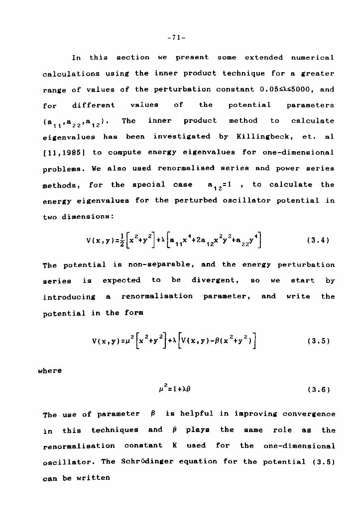
-71-
In this section we present some extended numerical
calculations using the inner product technique for a greater
range of values of the perturbation constant O.05~A~5000, and
for different values of the potential parameters
The inner product method to calculate
eigenvalues has been investigated by Killingbeck, et. al
[11,1985] to compute energy eigenvalues for one-dimensional
problems. We also used renormalised series and power series
methods, for the special case to calculate the
energy eigenvalues for the perturbed oscillator potential in
two dimensions:
( 3 • 4 )
The potential is non-separable, and the energy perturbation
series is expected to be divergent, so we start by
introducing a renormalisation parameter, and write the
potential in the form
2 [2 2] [ 2 2] V(x,y)=~ x +y +X V(x,y)-~(x +y ) ( 3 .5)
where
(3.6)
The use of parameter ~ is helpful in improving convergence
in this techniques and ~ plays the same role as the
renormalisation constant K used for the one-dimensional
oscillator. The Schrodinger equation for the potential (3.5)
can be written
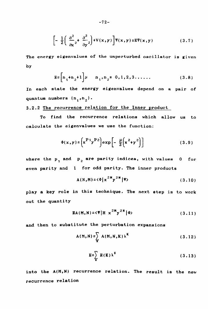
-72-
(3.7)
The energy eigenvalues of the unperturbed oscillator is given
by
(3.8)
In each state the energy eigenvalues depend on a pair of
quantum numbers (n1
,n2
).
3.2.2 The recurrence relation for the Inner product
To find the recurrence relations which allow us to
calculate the eigenvalues we use the function:
(3.9)
where the P1 and Pz are parity indices, with values 0 for
even parity and 1 for odd parity. The inner products
play a key role in this technique. The next step is to work
out the quantity
(3.11)
and then to substitute the perturbation expansions
A(M,N)=~ A(M,N,K)XK
(3.12)
E=? E(K)XK
(3.13)
into the A(M,N) recurrence relation. The result is the new
recurrence relation
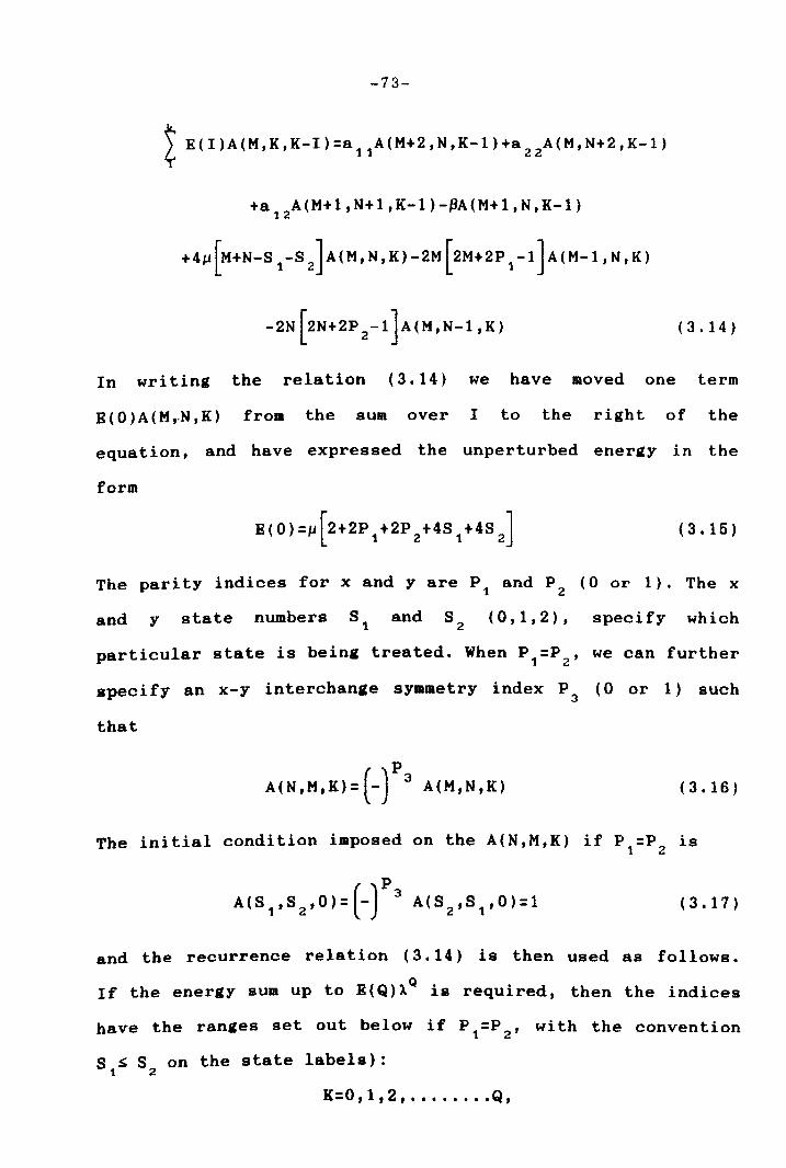
-73-
~ E(I)A(M,K,K-I)=a A(M+2,N,K-l)+a A(M,N+2,K-l) ~ 11 22
+a A(M+l,N+l,K-1)-~A(M+1,N,K-l) 12
(3.14)
In writing the relation (3.14) we have moved one term
B(O)A(MrN,K) from the sum over I to the right of the
equation, and have expressed the unperturbed energy in the
form
(3.15)
The parity indices for x and y are P1 and P2
(0 or 1). The x
and y state numbers S, and S2 (0,1,2), specify which
Particular state is being treated. When P =P , we can further 1 2
specify an x-y interchange symaetry index P3 (0 or 1) such
that
A(N,M,K)=(-)P 3 A(M,N,K) (3.16)
The initial condition imposed on the A(N,M,K) if P =P is 1 2
(3.17)
and the recurrence relation (3.14) is then used as follows.
If the energy sum up to E(Q)AQ is required, then the indices
have the ranges set out below if P1=P
2, with the convention
S1~ S2 on the state labels):
K=O, 1 t 2 t •••••••• Q,
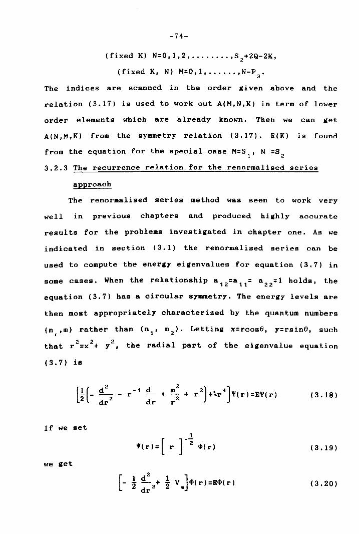
-74-
(fixed K) N=0,1,2, ........ ,8 +2Q-2K, 2
(fixed K, N) M=O,l, .•.••. ,N-P3'
The indices are scanned in the order given above and the
relation (3.17) is used to work out A(M,N,K) in term of lower
order elements which are already known. Then we can get
A(N,M,K) from the symmetry relation (3.17). E(K) is found
from the equation for the special case M=8 , N =8 1 2
3.2.3 The recurrence relation for the renormalised series
approach
The renormalised series method was seen to work very
well in previous chapters and produced hiahly accurate
results for the problems investigated in chapter one. As we
indicated in section (3.1) the renormalised series can be
used to compute the energy eigenvalues for equation (3.7) in
some cases. When the relationship a =a = a22
=1 holds, the 12 11
equation (3.7) has a circular symmetry. The energy levels are
then most appropriately characterized by the quantum numbers
(nr,m) rather than (n"
n 2 ). Letting x=rcos8, y=rsin8, such
2 2 2 that r =x + y , the radial part of the eigenvalue equation
(3.7) is
[!(-
If we set
we get
- 1 r
1
If(r)=[ r ]-2 "'(r)
(3.18)
(3.19)
(3.20)
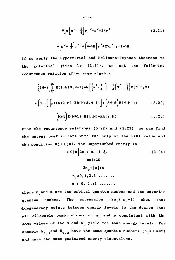
-75-
[ 2 1] -2 2 4 V
m= m - 4 r +r +2Ar ( 3 . 21)
[ 2 1] -2 ( ) 2 4 • m - 4 r + p-AK r +2Ar ,p=1+AK
If we apply the Hypervirial and Hellmann-Feynman theorems to
the potential given by (3.21), we get the following
recurrence relation after some algebra
+ (N + 2) [#lA ( N + 2 , M ) - KB ( N + 2 , M -1 ) ] + (2 N + 6 ) B ( N , M -1 ) (3.22)
(M+1)E(M+l)=B(4,M)-KA(2,M) (3.23)
From the recurrence relations (3.22) and (3.23), we can find
the energy coefficients with the help of the E(O) value and
the condition B(0,0)=1. The unperturbed energy is
E (0) = [2n r + I m I + 1] fii p=1+AK
2n +Im\=n r
n =0, 1 ,2, 3 , ••••••• r
m = 0,~1,~2, .•••.••
(3.24)
where n and m are the orbital quantum number and the magnetic r
quantum number. The expression (2n +lml+1) r
show that
ddegeneracy exists between energy levels to the degree that
all allowable combinations of n and m consistent wi th the r
same values of the m and n yield the same energy levels. For r
example E 1and Eo 2 have the same quantum numbers (n =0,m=2) 1, , r
and have the same perturbed energy eigenvalues.
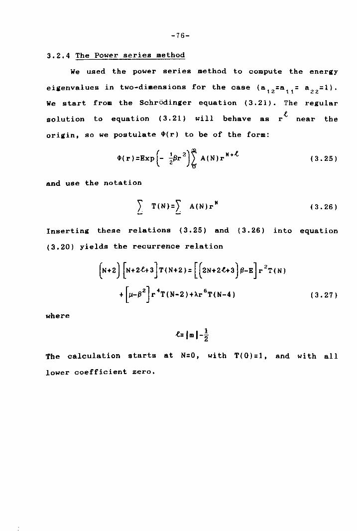
-76-
3.2.4 The Power series method
We used the power series method to compute the energy
eigenvalues in two-dimensions for the case (a =a = a~ =1). 12 11 ,,2
We start from the Schrodinger equation (3.21). The regular
solution to equation ( 3 . 21) will behave as ,f,
r near the
origin, so we postUlate ~(r) to be of the form:
(3.25)
and use the notation
J. T(N)=J. A(N)r" (3.26)
Inserting these relations (3.25) and (3.26) into equation
(3.20) yields the recurrence relation
[ 2] 4 6 + ~-p r T(N-2)+Xr T(N-4) (3.27)
where
The calculation starts at N:O, with T(0):1, and with all
lower coefficient zero.
-77-
3.2.5 Results and discussion
In this section we investigate and discuss the results
of the numerical calculations for the two-dimensional
systems. It is clear from our listed results in tables
(3.1-3.4) that the accuracy can be expected to decrease
rapidly as increases. Let us now turn to the
renormalisation constant (K) which is the heart of this
calculation for perturbative methods. We can see from the
results that the accuracy depends on the value of the
renormalised constant (K) • One continues to chanae the
renormalised constant until energy eiaenvalues of the best
required accuracy are obtained. The values of energy in table
(3.1) are for the case a12=a11=a22=1; we show some energies
for states (n ,n =0,1,2,3) and for 0.05SXS5000. The three 1 2
approaches work very well for two-dimensional oscillator, and
the results obtained by these methods are in good agreement
with each other. We observe that the three approaches yield a
high number of accurate digits (14) for the eigenvalues at
low values of X. For higher values of the perturbation
constant A the power series method gives more digits than the
inner product method with renormalised series.
One main di fference between the two perturbative
techniques lies in the values of the renormalised constant.
For the hypervirial approach the values of (K) increases as
the perturbation constant increase, while for the inner
product method the values of (K) decrease as the perturbation
constant increases. Also the hypervirial method can only work
for the case of a symmetric potential a =a =a =1 in which 11 22 12
-78-
the potential reduces to a one dimensional potential. The
inner product method deals with more general parameter
values, but still requires a =a 11 22'
since the equations used
exploit this symmetry to reduce computation. To get the
energy eigenvalues of Killingbeck and Jones [21,1980] it is ?
necessary to multiple our values by 2, since they used -v~ in
their Hamiltonian. All numerical calculations were done on
the leL (VME) system using double precision ari thmetic. A
good rate of convergence was achieved for all techniques and
was relatively insensitive to the choice of the state number.
Summarising our results we can say the following:
1. We succeeded in finding the energy eigenvalues for states
B 0,2
B 2,0
with
excellent accuracy in two-dimension even for high values of A
(O.05~~5000) and for different values of the potential
parameters (a =1,-1,0); 12
The set of tables
(3.1,3.2,3.3,3.4) cover a wide range values of (A).
2. We have found that the three methods work very well to
determine the energy eigenvalues, and give high accuracy. Our
resul ts are in good agreement with other reported resul ts
given by Killingbeck [21,1986], Hioe, et. al [22,1978], Ari
and Demiralp [20,1985].
3. We avoid the phenomenon of bogus convergence by computing
the energy eigenvalues for different values of the
renormalisation constant K. We believe that some of our
results .ay be improved in accuracy with a better choice of
K.

-79-
4. We calculated the energy eigenvalues for (68) states for
the symmetric potential 2 V(r)=(m - by using the
power series method for high quantum numbers (O~~400) and
(1~n~600). This approach produces (20) digits and the results
are presented in table (3.4). We wish to note that the
results yielded by the inner product were improved by using
Aitken extrapolation; it seem that extrapolation improves the
convergence of the perturbation series and gives extra
digits.
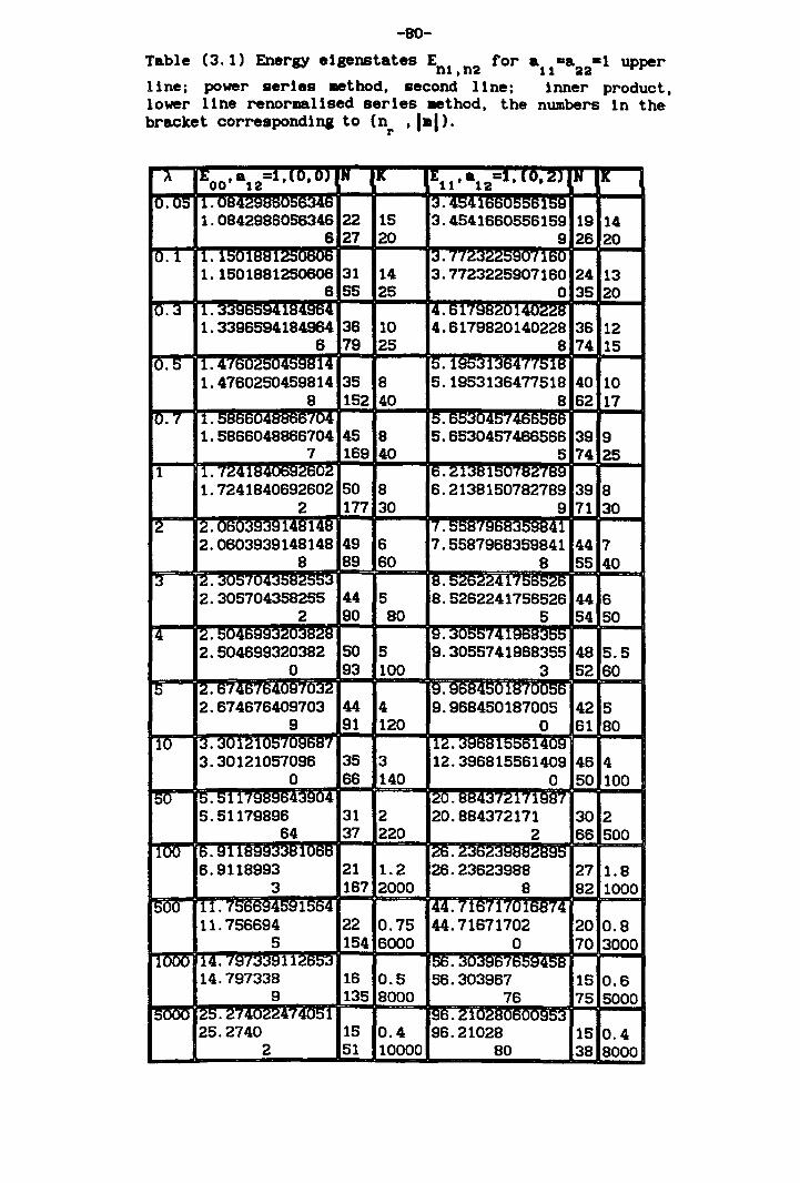
-80-
Table (3.1) Energy elgenstates E for a aa -I upper n1.na 11 22
line; power serles _thod. second Une; lnner product. lower llne renormallsed serles _thod. the numbers In the bracket corresponding to (n • I-P.
r
,\ IEoo' a12=I.l0. 0) IN lit iE11
• a1a
=l. lOt ZJ IN lit 10.05 IIJ 14 ... I~. 'l!:)'llSS055S159
1.0842986056346 22 15 3.4541660556159 19 14 6 27 20 9 26 20
10.1 11. 150 It:U:~ 13 • 11 , fltiU 1. 1501881250606 31 14 3.7723225907160 24 13
6 55 25 0 35 20 10 . 3 11. L' 14. 611::Jcsc;u14U~~K
1. 3396594184964 36 10 4.6179820140228 36 12 6 79 25 8 74 15
10.5 11. 41'" ;..> ... rl4!'iQ~14 15. 1953136477518 1.4760250459814 35 8 5.1953136477518 40 10
8 152 40 8 62 17 10.7 Il. ~ __ . .JfU4 15 . s!'S:m4!'i74
1.5866048866704 45 8 5.6530457466566 39 9 7 169 40 5 74 25
1 11. 7241R4 16. 21~t:nou, 0""'0;:;0
1. 7241840692602 50 8 6.2138150782789 39 8 2 177 30 9 71 30
12 12. llti' [(!of~~14B148 1'7. O:>I:S f!oltiH:i!'.l!ol~41
2.0603939148148 49 6 7.5587968359841 44 7 8 89 60 8 55 40
13 12 . .:sUO I 18 . 'D,1'f!jD5~D
2.305704358255 44 5 8.5262241756526 44 6 2 90 80 5 54 50
14 12 .!'in4 19 . .:suoo741 2.504699320382 50 5 9.3055741968355 48 5.5
0 93 100 3 52 60 15 12. 674676409 f u.:sc; 19 . rJltHUO!:)o
2.674676409703 44 4 9.968450187005 42 5 9 91 120 0 61 80
10 ~. 3012105'fU~l:)tSf .12. 3S6B155614U~ 3.30121051096 35 3 12.396815561409 46 4
0 66 140 0 50 100 50 5.5U', L":lQn4 !2U. HH4~'{2n18B'{
5.51179896 31 2 20. 884372171 30 2 64 37 220 2 66 500
100 0.~11 11066 20. "-:-'rl"-:-':
6.9118993 21 1.2 26.23623988 27 1.8 3 167 2000 8 82 1000
500 11. I 1564 :44.7167170168'(4 11.756694 22 0.75 44.71671702 20 0.8
5 154 6000 0 70 3000 [1000 14. f~f~~~:H 120!:)3 156. I I rl: i~4!jH
14.797338 16 0.5 56.303967 15 0.6 9 135 8000 76 75 5000
15000 12!:). 2141 :;';?~74051 190. 2102BI 25.2740 15 0.4 96.21028 15 0.4
2 51 10000 80 38 8000
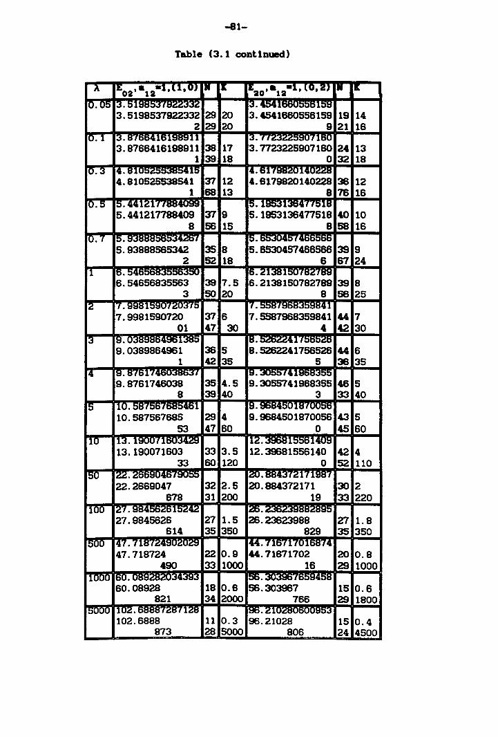
-81-
Table (3.1 continued)
A :1;02' -12-1 ,.,1.0J • ~ Eao '-12-1 ,(0.2J • I&.
10.05 ;3. ::S1tfts~~:H 3.454: i101l 3.5198537922332 29 20 3.4541660556159 19 14
2 29 20 9 21 16 10 . 1 .~. 87664ltn~1l 3. " IfltsU
3.8766416198911 38 17 3.7723225907160 24 13 139 18 0 32 18
10.3 4.8: ~1::; 4.61"ltftsot;U14n77N 4.810525538541 37 12 4.6179820140228 36 12
1 68 13 8 76 16 10 . 5 ::;.441Z1'11 .5. 1953136477518
5.44121n88409 37 9 5. 19531364n518 40 10 8 66 15 8 58 16
10.7 5. Ill~ 5.R..~R7·
5.93888565342 35 8 5.6530457466566 39 9 2 52 18 6 67 24
11 6. :6. Z1;381::;0·ftsot; ftstf 6.54656835563 39 7.5 6.2138150782789 39 8
3 50 20 8 56 25 12 7. 9981btfUlot;u",:> ., • ::l:)ts f II
7.9981590720 37 6 7.5587968359841 '" 7 01 47 30 4 42 30
1;3 ~. i1380 8. ~741. , ____
9.0389864961 36 5 8.5262241756526 '" 6 1 42 35 5 36 35
!4 ~. 8761-{4 If B.~/41
9.8761746038 35 4.5 9.3055741968355 46 5 8 39 40 3 33 40
5 10.~tsf~D' il 9. ~4 ... rllb,uu:>o 10.587567685 29 4 9.9684501870056 43 5
53 47 60 0 45 60 10 113. I~UUl'RfI~4~ 11Z.396815561409
13.190071603 33 3.5 12.39681556140 42 4 33 60 120 0 52 110
50 IZZ. ,.titi~1141'HtfU~ ZO.884;37Z171987 22.2669047 32 2.5 20.884372171 30 2
678 31 200 19 33 220 100 I·:n· i15Z4Z 1Z6·
27.9845626 27 1.5 26.23623988 ?:l 1.8 614 35 350 829 35 350
500 147. 7187?4: 144.716717016874 47.718724 22 0.9 44.71671702 20 0.8
490 33 1000 16 29 1000 1000 16U. 14~<1 156. ,
60.08928 18 O.B 66.303967 15 0.6 821 34 2000 766 29 1800
5000 110Z. OtststH c:ts 1128 IBB.Zll 102.6888 11 0.3 96.21028 15 0.4
873 28 5000 806 24 4500
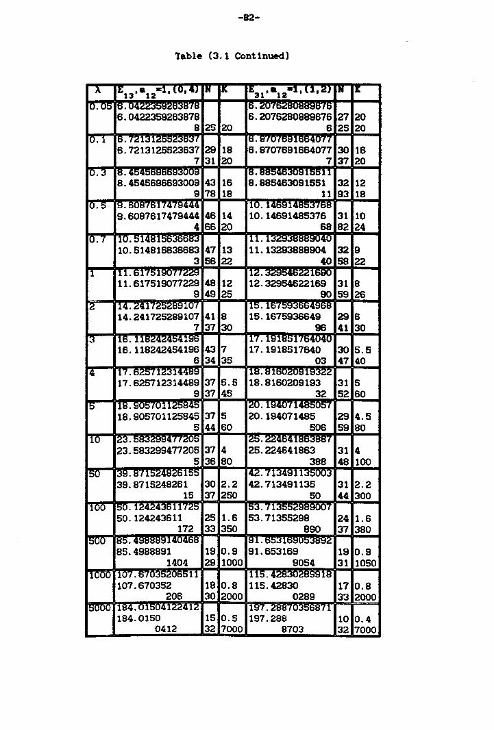
-82-
Table (3.1 Continued)
A 1!;13· a lZ-1• l0,4) IN IK 1t:31
,a12-1. (1,2) IN K
10.05 15 . 14' IIa 15.~UI 110
6.0422359263878 6.2076280889676 ZT 20 8 25 20 6 25 20
10.1 15. ~'Z13 ' I 16. l:HU lo~ltiti40T' 6.7213125523637 29 18 6.8707691664077 30 16
7 31 20 7 37 20 10 . 3 IB.4!"i 18. 110::»11
8.4545696693009 43 16 8.885463091551 32 12 9 78 18 11 93 18
10.5 :9.6087617479444 110. 145814B53"bts 9.6087617479444 46 14 10.14691485376 31 10
4 66 20 68 82 24 10.7 ,10.51481 Ill. 1:<1 141
10.514815636683 47 13 11.13293888904 32 9 3 56 22 40 58 22
11 11. ti175190', fi!.I!.'d 112. :.J7C1~M;:~ ~1680 11.617519077229 48 12 12.32954622189 31 8
9 49 25 90 59 26 ,2 14.24172528910" 115. 15',
14.241725289107 41 8 15.1675936648 29 6 7 37 30 96 41 30
3 It:;. 1 'R7474R~18D In. ISU:lo17H404I 16.118242454196 43 7 17.1918517640 30 5.5
6 34 35 03 47 40 4 17. 5257123144B'd I1B.Bll Il8322
17.625712314489 37 5.5 18.8160209193 31 5 9 37 45 32 52 60
5 IB.~u;:),1J1.25S40 120.1940714 ___ -" 18.905701125845 37 5 20.194071485 29 4.5
5 44 60 506 59 80 10 23. ~R";f7QQ, : ( ( .::u;:) 125. 774R41 ,
23.583299477205 37 4 25.224641863 31 4 5 36 80 388 48 100
50 39. B'(1~~4B26155 142.7134911 39.8715248261 30 2.2 42.713491135 31 2.2
15 37 250 50 44 300 100 150. 1 ?4?4~R 11725 153. 71: 1 I
50.124243611 25 1.6 53.71355298 24 1.6 172 33 350 890 37 380
500 IS::». 4n4RR 91.6531 85.4988891 19 0.9 91.653169 19 0.9
1404 29 1000 9054 31 1050 1000 1101. 0 ( "'~11 115. H~~18
107.670352 18 0.8 115.42830 17 0.8 206 30 2000 0289 33 2000
15000 1184.01504122412 : 197 . .::aa I u,,;:)oa (1 184.0150 15 0.5 197.288 10 0.4
0412 32 7000 8703 32 7000
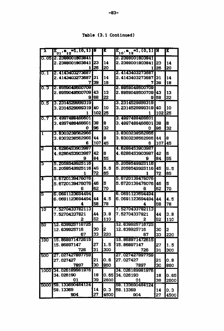
-83-
Table (3.1 Continued)
A I£Ol,a12-I,IU,1J IN 11: £10,a12-1,IU.1J I" 1& [0.05 I~· 11Rn~41 -- ~. _____ JIRfI:<lR~l
2.2388001803841 23 14 2.2388001803841 23 14 1 26 20 1 26 20
10.1 1~·414~ ;f~OI I~. 41434[ ;, "CO,
2.4143403273687 31 14 2.4143403273687 31 14 7 39 18 7 39 18
10.3 I~· "v;:, I~· - "v::. 2.8959049500709 43 13 2.8959049500709 43 13
9 68 22 9 68 22 10.5 13.Z314 119 13.2314 118
3.2314529999319 40 10 3.2314529999319 40 10 1 102 25 1 102 25
10.7 13.499"1 11 13 . 48874 01 3. 49974S8468601 38 8 3.4997488466601 38 8
0 96 32 0 96 32 1 13 . ~ 13 .
3. 8303238562966 44 8 3.8303238562966 44 8 6 107 45 6 107 45
12 14. R if 14 . R7.~R4 if 4.6286453903987 42 6 4.6286453903987 42 6
9 84 55 9 84 55 [3 15. :oI'!i116 1::1· .25115
5.2058549925116 45 5.5 5.2058549925116 45 5.5 1 72 65 1 72 65
14 15.5-/ZOl394'fDUfD 15. 57~01384'fDVfD 5.6720139476076 46 5 5.6720139476076 46 5
6 62 70 6 62 70 15 15.05S11~UA4 14 Its. 05S112:;1R~144C4
6.0691123694494 44 4.5 6.0691123694494 44 4.5 4 58 78 4 58 78
-lO 7. 52704~ns~113 7. 5270433'f cs~ 113
7.52704331821 44 3.8 7.52704337821 44 3.8 2 52 110 2 52 110
50 11~. 1/167~ 11~. 11t:H~o
12.639925716 30 2 12.639925716 30 2 67 33 220 67 33 220
flOO 115. 868S714-/~15 115. CSDCS::' fl4-'~ts It; 15.86897147 27 1.5 15.86897147 27 1.5
726 31 300 726 31 300 [SOO 127. 0~74Zf~f to::. 127. U~(4~'fCS::'f fO~
27.027427 21 0.8 27.027427 21 0.8 7897 30 860 7897 30 860
1000 134.02518SS8UH5 134. 0~518SS8U:fft) 34.026190 18 0.65 34.026190 18 0.65
01 39 2600 01 39 2600 15000 IOH.1 LJ(~1~4 158. 1 L~~l~'1
58.13369 14 0.3 58.13369 14 0.3 904 27 4500 904 27 4500
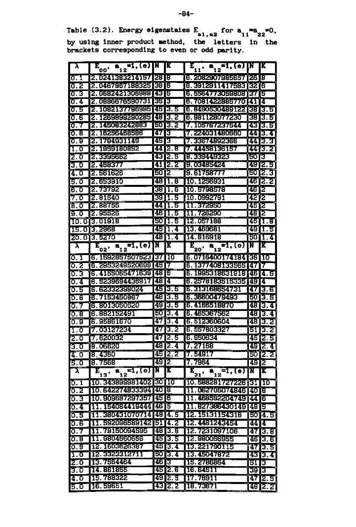
-84-
Table (3.2). Energy elgenstates E ~or a -a -0. D1.D2 11 22
by using inner product ethod. the letters In the brackets corresponding to even or odd parity.

-85-
Table (3.2 Continued)
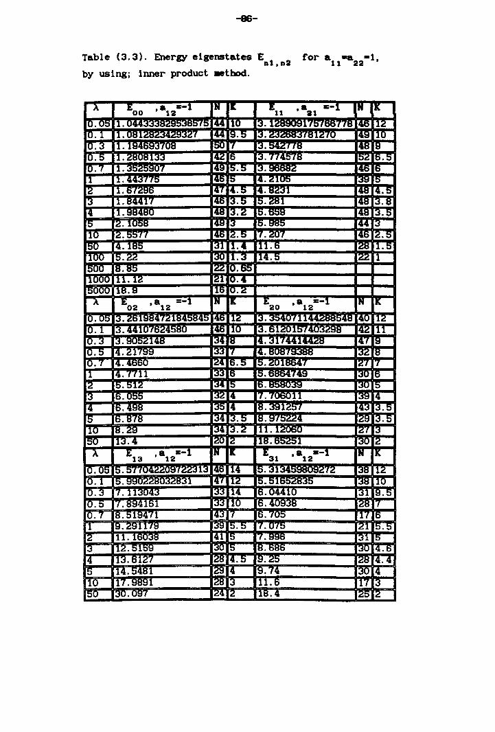
-86-
Table (3.3). Energy elgenstates E 1 2 for a -a -1, D ,D 11 22
by uslngj hmer product aetbod.
A Eoo a =-1 • 12
IN 11: El1 a 11:-1 • al N K
"0.05 1.n4 !;,~ 144 10 3. , 11'1:;' IDD I la 46 12 0.1 1. 08 7R7-.r1l7Q-'(~" l'!'! 9.5 13. IIo1Z70 i49 10 0.3 1. U:J4t)93'fua 150 7 13.542''-'8 148 9 0.5 I.Z8U8133 14Z 6 :3. 77,!578 10Z 6.5 "0.7 1. 'I 149 5.5 3. 146 6 1 1.443775 146 l~ 4.?.!Q5 39 5 2 1. D It:tlD 147 14.5 4.8231 4l! 4.0 3 1. 84417 l46 3.0 o.ZBl 48 3.8 4 1. ~w4Rr 148 3.2 5.659 ~8 3.5 5 2.1()~ 149 3 '5.985 44 13 10 2.5577 14t.i Z.5 ;", ZO" 46 Z.5 50 4.185 131 1.4 il1.6 28 1.5 100 5.Z2 ~. 1.3 114.5 ,22 1 500 8.80 IZZ 0.65 1000 11.12 l?l. 0.4 5UUU IB.9 116 U.2
i\ E02 a =-1 , 12 IN I: 1:20
a =-1 • 12
N K
0.U5 3.z6198472' 146 12 13. 3540711 llll i40 12
0.1 3.441076?4~Rn lilt) 10 13. 61Z015741 :4;.;o~H 142 111 0.3_ 13.905Z148 134 B i4.3H4414428 47 9 10.5 14.ZHSS 33 7 ~·avan:t~ 3Z 8 rO.7 14.4t)~ Z4 16.5 5.Z01864'f 2J "I
1 4. Till 133 6 0.~!49 30 6 2 5.51Z 134 5 16. ~ P 3 6.055 ~. 4 "I. '/06011 39 4 4 6.498 135 4 18.39125"1 ,43 :3.5 5 6.878 @! 3.5 18. tl/:;'U;~ :2S 13.5 10 8.29 134 13._? 111·12060 Z"I :3
150 113.4 jZO IZ :18.65251 3U 2 i\ 1:13 a =-1
• 12 N 11: 1:31 a =-1
• 12 N K
10.UO 15. 57~ .4?~IJ~f"J13 46 114 5.3' "l.ll""QRrlQ~7Z 3~ 12 U.l 15. tI: ?R~1 14" 11Z 15.51 l"!o!\;.;oH:4!\ 3~ 10 0,3 7.113043 133 14 16.0441U .31 i9.5 0.5 7.894161 ~ 10 16. 4mnR IZB 7
10·Z 18.5194"'1 ~ 7 16.705 1'1 16 i 1 19. ZSll'~ 39 15.5 7.075 ZI 15.5
12 11. 16038 41 15 7.996 31 5 13 lZ.51bS ,30 15 8.686 3U 4.6
14 113.6127 '2H 14.5 9.?~ 28 4.4
15 11~. 5481 .~ [4 9.7,! 3U 4
110 117. stnn ~ 13 11.6 11 3 150 130. mu 124 12 J,8.4 25 2
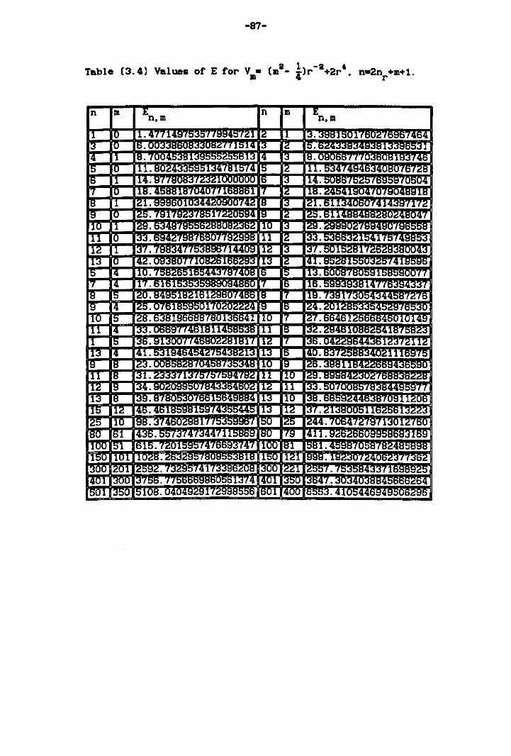
-87-
2 1 -2 , Table (3.4) Values of E for V.- (m - i)r +2r. n-2nr +m+1.
-88-
3.3 THREE AND N DIMENSIONAL PROBLEMS
3.3.1 Introduction
J.Killingbeck [22,1985] has used the Hill determinant
method to calculate the energy eigenvalues for a
three-dimensional oscillator and also investigated all
spherically symmetric states in any dimension (N:1,2,3
•••• 320). He computed the energy eigenvalues and expectation
2 . 1 .-1 4 d -1 4 values such as <r > for potent1a s -\. r an N r and gave
resul ts of high accuracy. We extended our numerical
calculations for higher powers of the perturbation index
(2N:4,6,8), and for a wide range of values of angular
momentum, perturbation parameter, and state number. We used
two methods to produce our results for this problem, the
renormalised series method and the power series method. The
radial part of the three-dimensional Schr6dinger equation can
be written conventionally in the form
(3.28)
where (t) is the angular momentum, and the energies of
unperturbed levels are
(3.29)
where n is the principal quantum number, which can be
expressed as
(3.30)
Here n is called the radial quantum number. The energy values r
include zero-point energy 3 corresponding to the three
degrees of freedom. n is seen to be even or odd according as
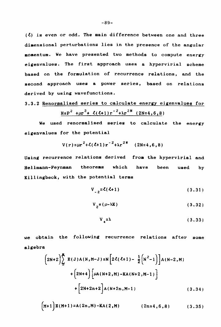
-89-
(t) is even or odd. The main difference between one and three
dimensional perturbations lies in the presence of the angular
momentum. We have presented two methods to compute energy
eigenvalues. The first approach uses a hypervirial scheme
based on the formulation of recurrence relations t and the
second approach uses a power series, based on relations
derived by using wavefunctions.
3.3.2 Renormalised series to calculate energy eigenvalues for
2 2 -2 2N H:P +~r + t(t+l)r +Ar (2N:4,6,8)
We used renormalised series to calculate the energy
eigenvalues for the potential
2 -2 2N V(r):~ +t(t+l)r +Ar (2N:4,6,8)
Using recurrence relations derived from the hypervirial and
Hellmann-Feynman theorems which have been used by
Killingbeck, with the potential terms
v :t(t+l) -2
V :A 4
( 3 . 31)
(3.32)
(3.33)
we obtain the following recurrence relations after some
algebra
(2N+2)~ E(J)A(N,M-J):N[2l.(l.+1)- ~(N2-1)JA(N-2'M)
+ ( 2 N + 4) [1lA ( N + 2 , M ) - KA ( N + 2 , M - 1 ) ]
+ [2N+2n+2]A(N+2n,M-l)
(M+l)E(M+l):A(2n,M)-KA(2,M) (2n:4,6,8)
(3.34)
(3.35)
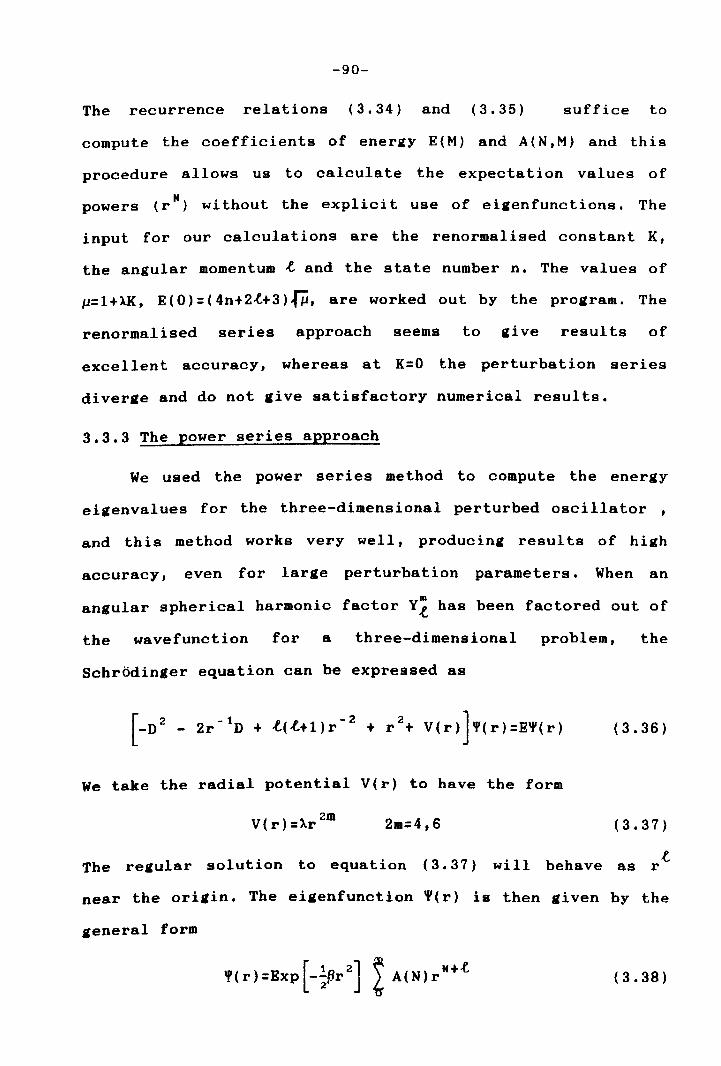
-90-
The recurrence relations (3.34) and (3.35) suffice to
compute the coefficients of energy E(M) and A(N,M) and this
procedure allows us to calculate the expectation values of
powers (rH) without the explicit use of eigenfunctions. The
input for our calculations are the renormalised constant K,
the angular momentum ~ and the state number n. The values of
~=l+AK, E(O)=(4n+2~+3)~, are worked out by the program. The
renormalised series approach seems to give results of
excellent accuracy, whereas at K=O the perturbation series
diverge and do not give satisfactory numerical results.
3.3.3 The power series approach
We used the power series method to compute the energy
eigenvalues for the three-dimensional perturbed oscillator ,
and this method works very well, producing resul ts of high
accuracy, even for large perturbation parameters. When an
angular spherical harmonic factor Yt has been factored out of
the wavefunction for a three-dimensional problem, the
Schrodinger equation can be expressed as
-D - 2r D + ~(~+l)r + r + V(r) '(r)=E'(r) [
2 -1 g g -2 2 ]
We take the radial potential V(r) to have the form
2m V(r)=:A.r 2m=4,6
The regular solution to equation (3.37) will behave
(3.36)
(3.37)
~ as r
near the origin. The eigenfunction '(r) is then given by the
general form
[ 1 21 ~ H+~
'(r)=Exp -;iJr J ~ A(N)r (3.38)
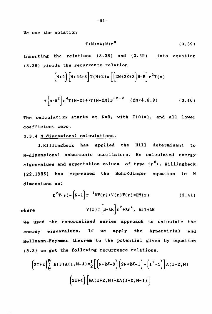
-91-
We use the notation
T(N)=A(N)r" (3.39)
Inserting the relations (3.38) and (3.39) into equation
(3.36) yields the recurrence relation
+ p-~ r T(N-2)+AT(N-2M)r [ 2] 4 2" + 2 (2M=4,6,8) (3.40)
The calculation starts at N=O, wi th T( 0) = 1, and all lower
coefficient zero.
3.3.4 N dimensional calculations.
J.Killingbeck has applied the Hill determinant to
N-dimensional anharmonic oscillators. He calculated energy
eigenvalues and expectation values of type <rH>. Killingbeck
[22,1985] has expressed the Schrodinger equation in N
dimensions as:
( 3 .41 )
where
We used the renormalised series approach to calculate the
energy eigenvalues. If we apply the hypervirial and
Hellmann-Feynman theorem to the potential given by equation
(3.3) we get the following recurrence relations.
( 2 I + 2 ) ~ E ( J ) A ( I , M- J ) = i [ (N + 2,(,-3 ) (2 N + 2,(,- 1 ) - (I 2 - 1) ] A ( 1-2 , M )
( 2 I + 4) [#lA ( 1+2 , M ) - KA ( I + 2 , M - 1 ) ]
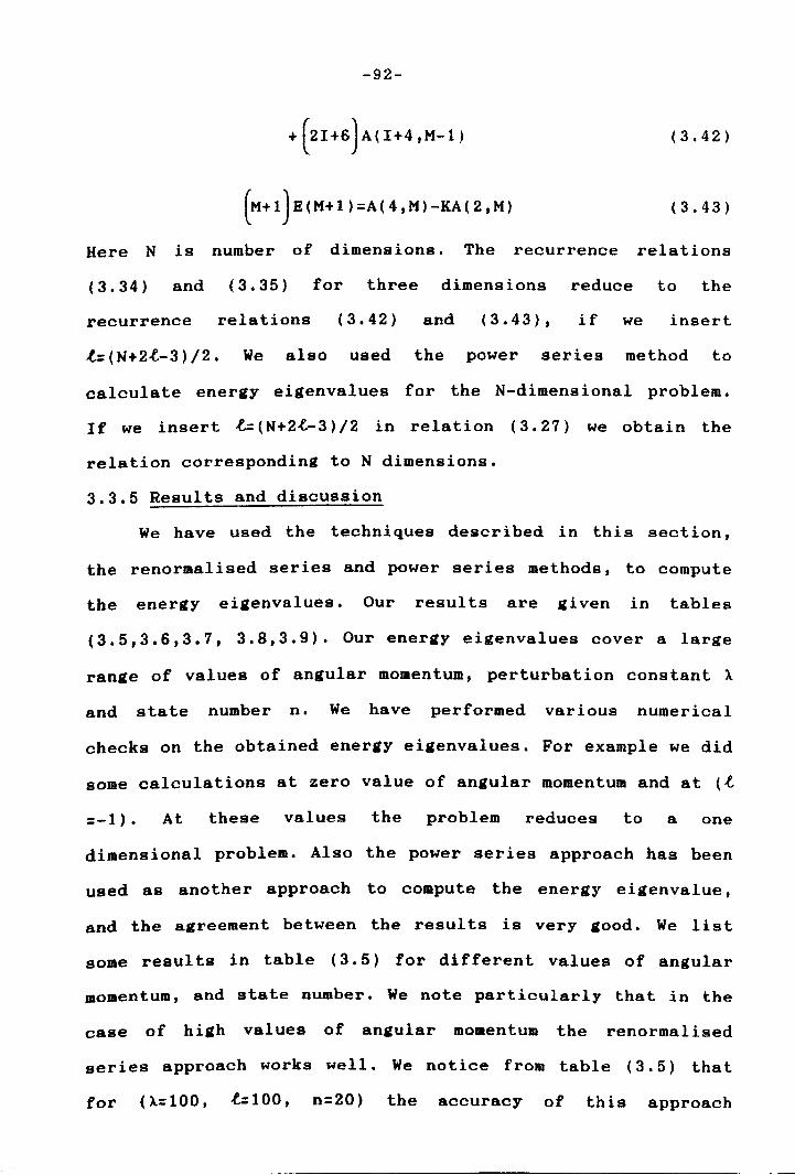
-92-
+ (21+6 )A( 1+4 ,M-1) (3.42 )
(M+1)E(M+1)=A(4,M)-KA(2,M) ( 3 . 43 )
Here N is number of dimensions. The recurrence relations
(3.34) and (3.35) for three dimensions reduce to the
recurrence relations (3.42) and (3.43), if we insert
~=(N+2~-3)/2. We also used the power series method to
calculate energy eigenvalues for the N-dimensional problem.
If we insert ,f,:(N+2.t-3)/2 in relation (3.27) we obtain the
relation corresponding to N dimensions.
3.3.5 Results and discussion
We have used the techniques described in this section,
the renormalised series and power series methods, to compute
the energy eigenvalues. Our results are given in tables
(3.5,3.6,3.7, 3.8,3.9). Our energy eigenvalues cover a large
range of values of angular momentum, perturbation constant A
and state number n. We have performed various numerical
checks on the obtained energy eigenvalues. For example we did
some calculations at zero value of angular momentum and at ({
=-1). At these values the problem reduces to a one
dimensional problem. Also the power series approach has been
used as another approach to compute the energy eigenvalue,
and the agreement between the results is very good. We list
some results in table (3.5) for different values of angular
momentum, and state number. We note particularly that in the
case of hiJth values of angular momentum the renormalised
series approach works well. We notice from table (3.5) that
for (X=100, .f..::l00, n=20) the accuracy of this approach
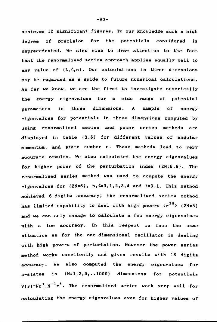
-93-
achieves 12 significant figures. To our knowledge such a high
degree of precision for the potentials considered is
unprecedented. We also wish to draw attention to the fact
that the renormalised series approach applies equally well to
any value of (X, t, n). Our calculations in three dimens ions
may be regarded as a guide to future numerical calculations.
As far we know, we are the first to investigate numerically
the energy eigenvalues for a wide range of potential
parameters in three dimensions. A sample of energy
eigenvalues for potentials in three dimensions computed by
using renormalised series and power series methods are
displayed in table (3.6) for different values of angular
momentum, and state number n. These methods lead to very
accurate results. We also calculated the energy eigenvalues
for higher power of the perturbation index (2N=6, 8). The
renormalised series method was used to compute the energy
eigenvalues for (2N=6), n,t:0,1,2,3,4 and X=0.1. This method
achieved 6-digits accuracy; the renormalised series method
has limited capability to deal with high powers <r 2N) (2N=8)
and we can only manage to calculate a few energy eigenvalues
with a low accuracy. In this respect we face the same
si tuation as for the one-dimensional oscillator in deal ing
wi th high powers of perturbation. However the power series
method works excellently and gives resul ts wi th 16 digi ts
accuracy. We also computed the energy eigenvalues for
s-states in (N:1, 2,3, •• 1000) dimensions for potentials
4 -1 4 V(r)=Nr,N r. The renormalised series work very well for
calculating the energy eigenvalues even for higher values of

-94-
N. The energy eigenvalues are com pared wi th corresponding
ones obtain by the power series method and listed in table
(3.8). The agreement of our results with those of Killingbeck
is good.
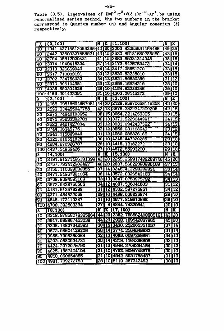
-95-2 2 -2 4 Table (3.5). Eigenvalues of H=P +r +t(t+l)r +Ar ,by using
renormalised series method, the two numbers in the bracket correspond to Quantum number (n) and Angular momentum (t) respectively.
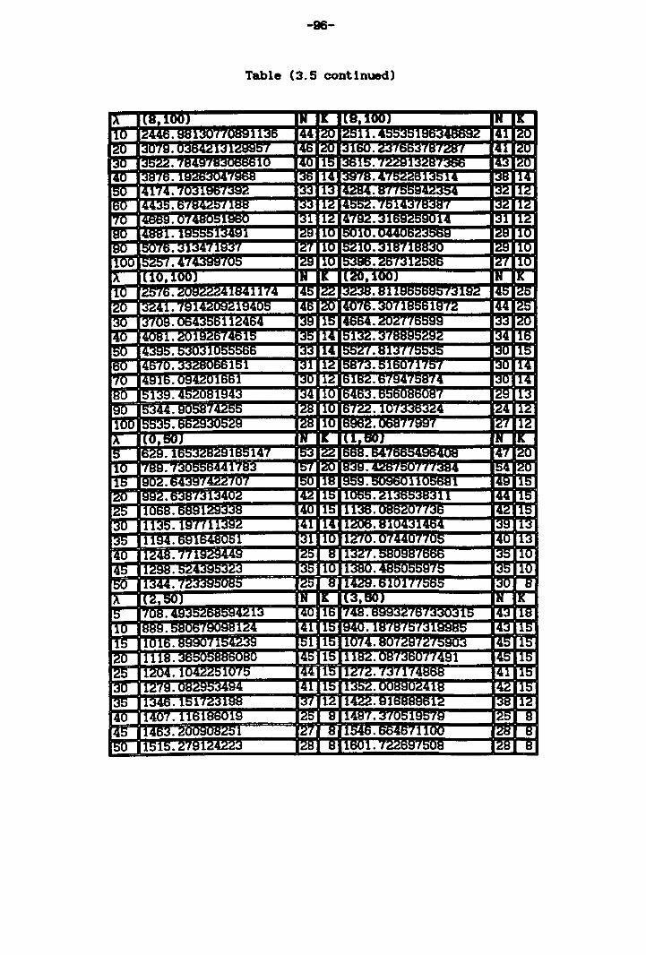
-96-
Table (3.5 continued)
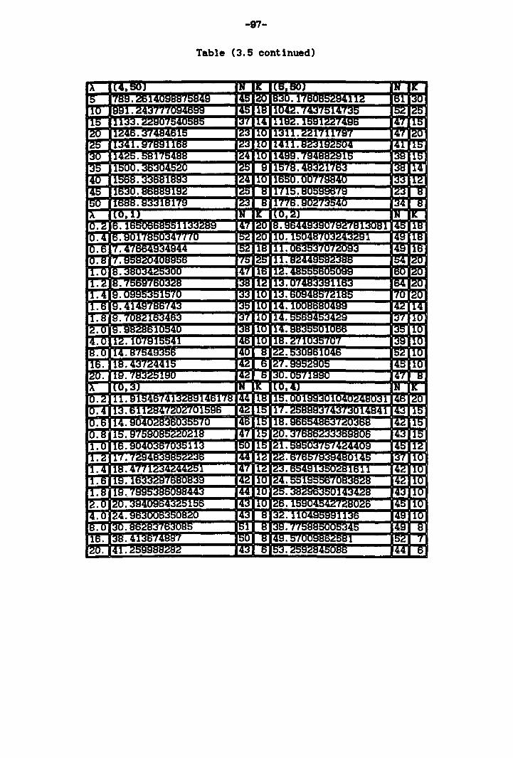
-97-
Table (3.5 continued)
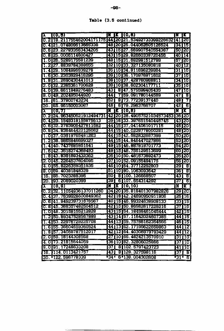
-98-
Table (3.5 continued)
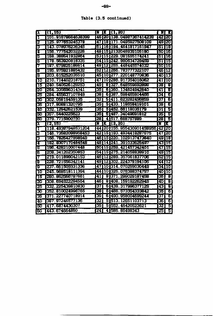
-99-
Table (3.5 continued)
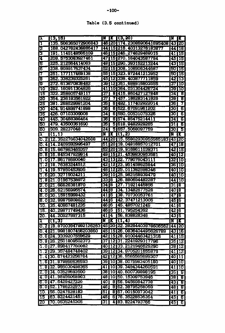
-100-
Table (3.5 continued)
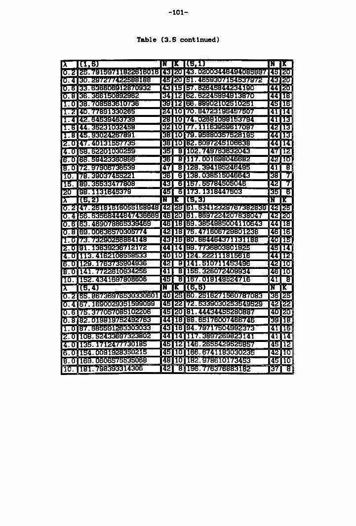
-101-
Table (3.5 continued)
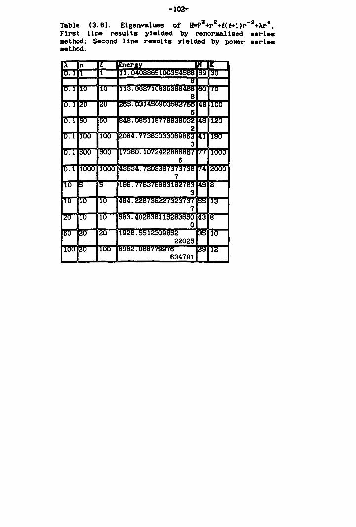
-102-
Table (3.6). Ei ge nva 1 ues of H-p2+r 2+t (t+l)r-2+Ar'. First line results yielded by renormalised series method; Second line resul ta yielded by power series method.
634781
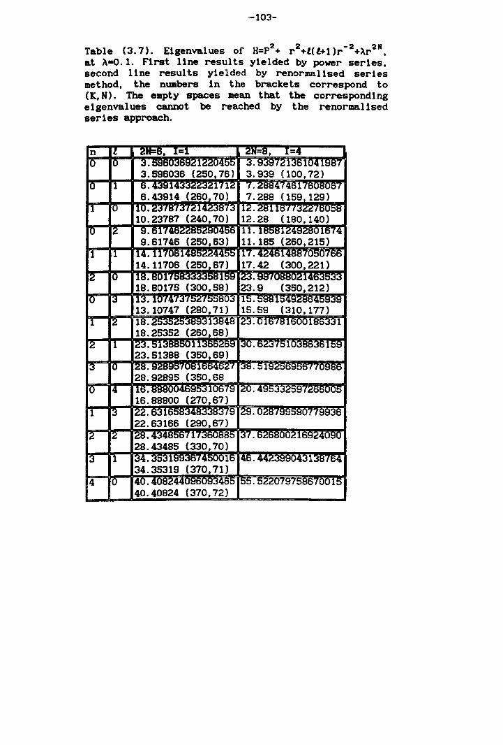
-103-
Table (3.7). Eigenvalues of H=p2+ r 2 +t(t+l)r -2+~r2N, at ~-o.I. First line results yielded by power series, second line results yielded by renormalised series method, the numbers in the brackets correspond to (K, N). The empty spaces mean that the corresponding eigenvalues cannot be reached by the renormalised series approach.
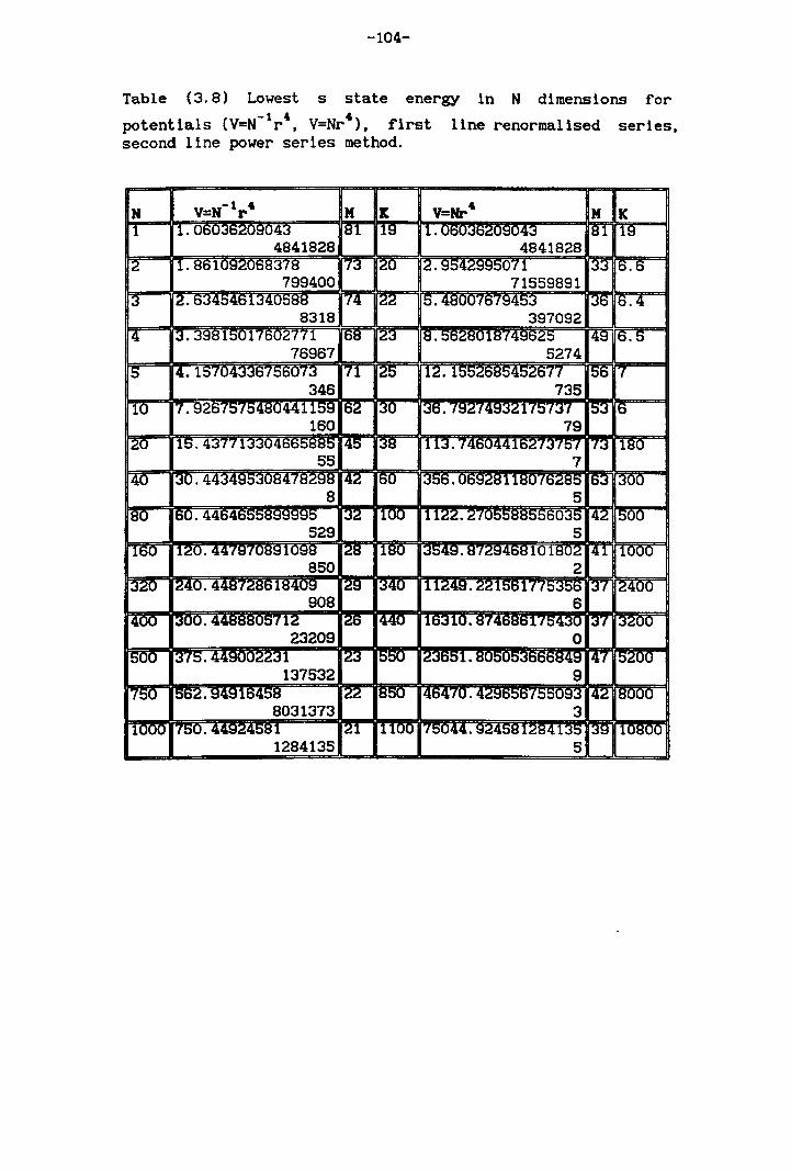
-104-
Table (3.8) Lowest s state energy in N dimensions for -1 , ,
potentials (V=N r, V=Nr >, first line renormalised series, second line power series method.
1284135 5
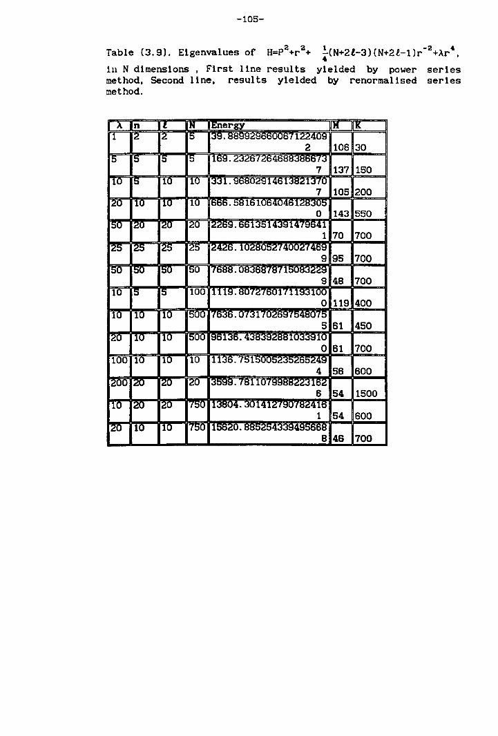
-105-
2 2 1 -2 " Table (3.9). Eigenvalues of H=P +r + -(N+2l-3)(N+2l-1)r +Ar •
" in N dimensions. First line results yielded by power series method, Second line, results yielded by renormalised series method.
700
700
700
450
700
600
1500
600
B 46 700
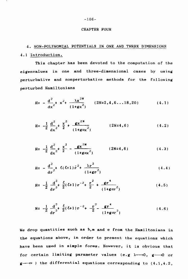
-106-
CHAPTER FOUR
4. NON-POLYNOMIAL POTENTIALS IN ONE AND THREE DIMENSIONS
4.1 Introduction.
This chapter has been devoted to the computation of the
eigenvalues in one and three-dimensional cases by using
perturbative and nonperturbative methods for the following
perturbed Hamiltonians
H= - (2N=2,4,6 ••. 18,20)
1 d 2 2 H= -- - + ~ +
2 dx2 2
2" gx 2 (l+gax )
(2N=4,6)
? 2 2N H=
1 d W x gx (2N=4,6) -- - + 2- .,
2 dx2 ( l+gax"')
.., 2
H= d'" t(.t+ 1) r 2 + Ar
- -+ 2 2
dr (l+gr )
1 d 2 t t -2
2 4 E-+ gr
H= -"2 -+ 2( +1)r + 2 2 ..,
dr (t+gar W
,
.., 2 4 1 d'" t -2 r gr
H= --2 -.., + i( t+ 1) r + -2 - 2
dr w (l+gar )
( 4 • 1 )
( 4 • 2 )
( 4 . 3 )
( 4 .4)
( 4 . 5 )
( 4 .6)
We drop quantities such as h,m and e from the Hamiltonians in
the equations above, in order to present the equations which
have been used in simple forms. However, it is obvious that
for certain limi ting parameter values (e. g A~O, g~ or
g~ ) the differential equations corresponding to (4.1,4.2,
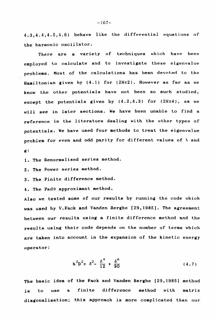
-107-
4.3,4.4,4.5,4.6) behave like the differential equations of
the harmonic oscillator.
There are a variety of techniques which have been
employed to calculate and to investigate these eigenvalue
problems. Most of the calculations has been devoted to the
Hamiltonian given by (4.1) for (2N=2). However as far as we
know the other potentials have not been so much studied,
except the potentials given by (4.2,4.3) for (2N=4), as we
will see in later sections. We have been unable to find a
reference in the literature dealing with the other types of
potentials. We have used four methods to treat the eigenvalue
problem for even and odd parity for different values of ~ and
g:
1 • The Renormalised series method.
2. The Power series method.
3. The Finite difference method.
4. The Pade approximant method.
Also we tested some of our results by running the code which
was used by V.Fack and Vanden Berghe [29,1985]. The agreement
between our results using a finite difference method and the
results using their code depends on the number of terms which
are taken into account in the expansion of the kinetic energy
operator:
( 4 . 7 )
The basic idea of the Fack and Vanden Berghe [29,1985] method
is to use a finite difference method with matrix
diagonalisation; this approach is more complicated than our
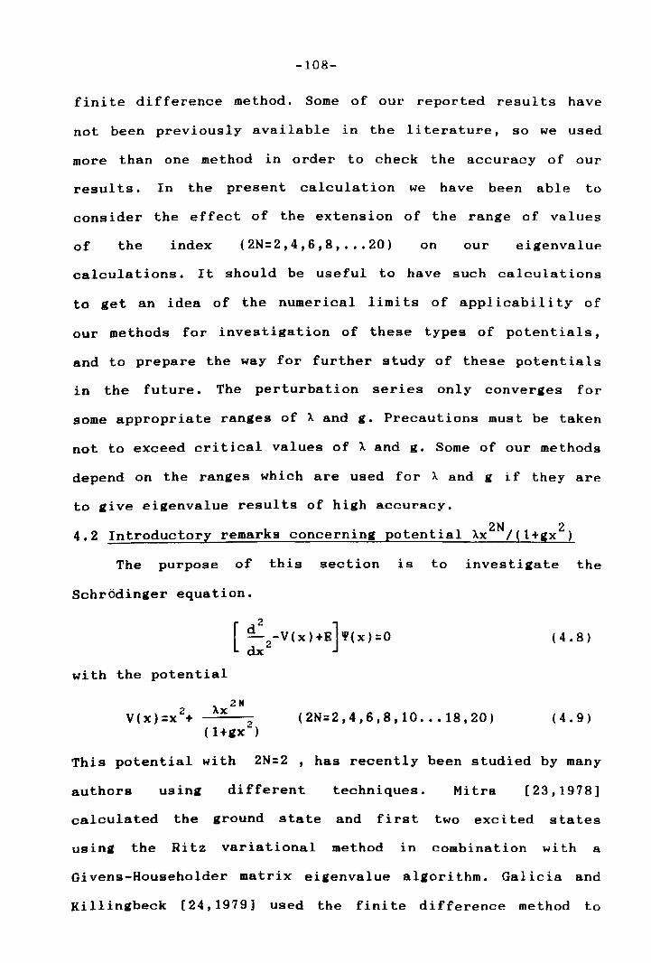
-108-
finite difference method. Some of our reported results have
not been previously available in the literature, so we used
more than one method in order to check the accuracy of our
resul ts. In the present calculation we have been able to
consider the effect of the extension of the range of values
of the index (2N=2,4,6,8, ... 20) on our eigenvalue
calculations. It should be useful to have such calculations
to get an idea of the numerical limits of applicability of
our methods for investigation of these types of potentials,
and to prepare the way for further study of these potentials
in the future. The perturbation series only converj(es for
some appropriate ranges of A and g. Precautions must be taken
not to exceed critical values of X and g. Some of our methods
depend on the ranges which are used for A and g if they are
to give eigenvalue results of high accuracy.
2N 2 4.2 Introductory remarks concerning potential Xx l(l+gx)
The purpose of this section is to investigate the
Schrodinger equation.
with the potential
2 V(x)=x +
AX2N
2 (l+gx )
( 4 .8)
(2N=2,4,6,8,10 ••• 18,20) ( 4 .9)
This potential with 2N=2, has recently been studied by many
authors usinj( different techniques. Mitra [23,1978]
calculated the ground state and first two exci ted states
using the Ritz variational method in combination with a
Oi vens-Householder matrix eigenvalue algori thm. Oalicia and
Killingbeck [24,1979] used the finite difference method to
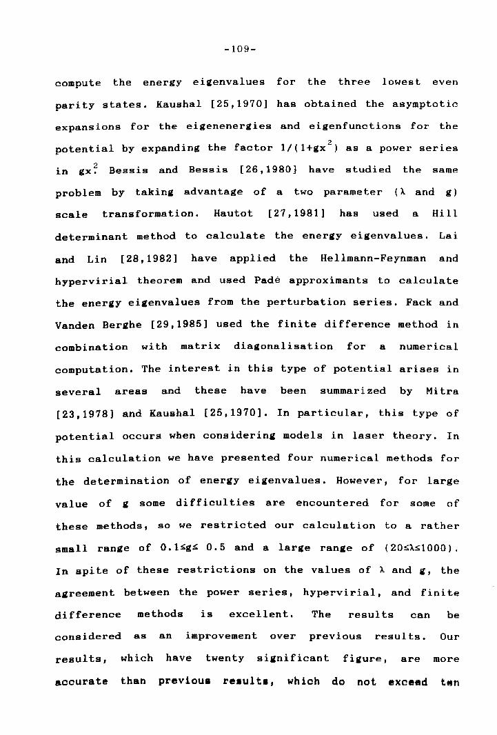
-109-
compute the energy eigenvalues for the three lowest even
parity states. Kaushal [25,1970] has obtained the asymptotic
expansions for the eigenenergies and eigenfunctions for the ?
potential by expanding the factor 1/(1+gx~) as a power series
in 2 gx. Bessis and Bessis [26,1980] have studied the same
problem by taking advantage of a two parameter (A and g)
scale transformation. Hautot [27,1981] has used a Hill
determinant method to calculate the energy eigenvalues. Lai
and Lin [28,1982] have applied the Hellmann-Feynman and
hypervirial theorem and used Pade approximants to calculate
the energy eigenvalues from the perturbation series. Fack and
Vanden Berghe [29,1985] used the finite difference method in
combination with matrix diagonalisation for a numerical
computation. The interest in this type of potential arises in
several areas and these have been summarized by Mitra
[23,1978] and Kaushal [25,1970]. In particular, this type of
potential occurs when considering models in laser theory. In
this calculation we have presented four numerical methods for
the determination of energy eigenvalues. However, for large
value of i some difficulties are encountered for some of
these methods, so we restricted our calculation to a rather
small range of O. 1:s:g:s: 0.5 and a large range of (20:S:A:s:l 000) .
In spite of these restrictions on the values of A and i, the
agreement between the power series, hypervirial, and finite
difference methods is excellent. The results can be
considered as an improvement over previous results. Our
results, which have twenty significant figure, are more
accurate than previoua reaulta, which do not exceed ten
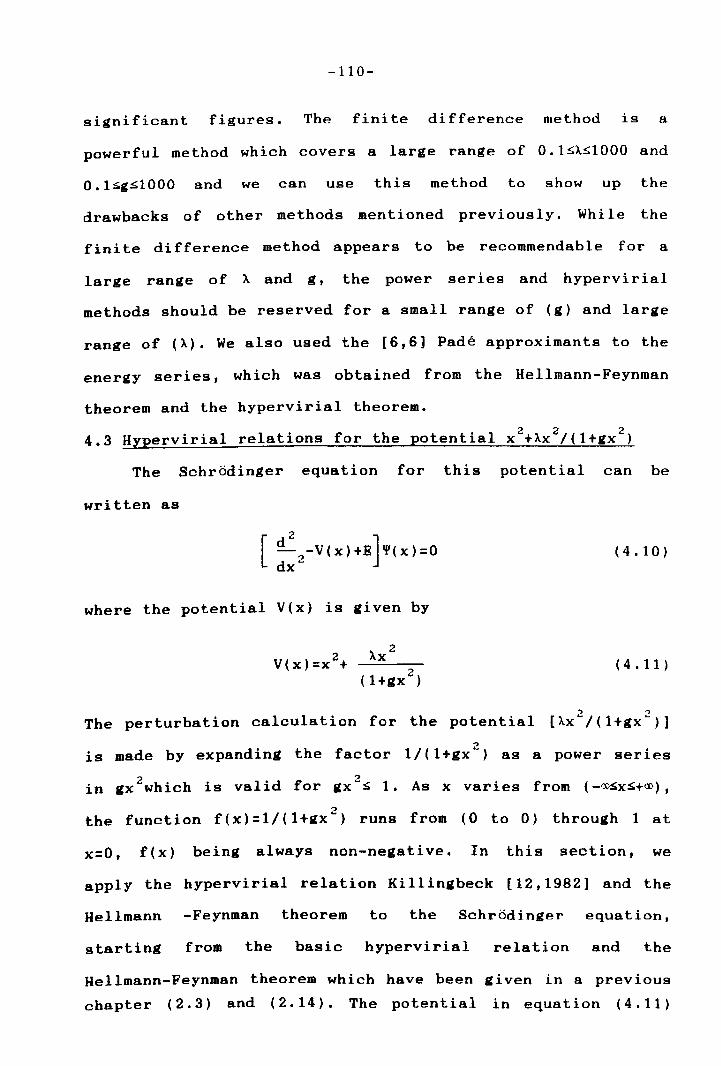
-110-
significant figures. The finite difference method is a
powerful method which covers a large range of 0.1~~~1000 and
O.1~g~1000 and we can use this method to show up the
drawbacks of other methods mentioned previously. Whi le the
fini te difference method appears to be recommendable for a
large range of A and g, the power ser ies and hypervi r ial
methods should be reserved for a small range of (g) and large
range of (A). We also used the [6,6] Pade approximants to the
energy series, which was obtained from the Hellmann-Feynman
theorem and the hypervirial theorem. ') 2 2
4.3 Hypervirial relations for the potential X~+AX /(1+gx )
The Schrodinger equation for this potential can be
written as
where the potential V(x) is given by
2 V(x) =x +
(4.10)
(4.11)
') .~
The perturbation calculation for the potential [Ax~/(1+gx~)]
2 is made by expanding the factor 1/(1+gx ) as a power series
in gx 2 which is valid for gX2~ 1. As x varies from (-':o~x~+<l»,
the function f(x)=1/(1+gx2
) runs from (0 to 0) through 1 at
x=O, f(x) being always non-negative. In this section, we
apply the hypervirial relation Killingbeck [12,1982] and the
Hellmann -Feynman theorem to the Schrodinger equation,
starting from the basic hypervirial relation and the
Hellmann-Feynman theorem which have been given in a previous
chapter (2.3) and (2.14). The potential in equation (4.11)
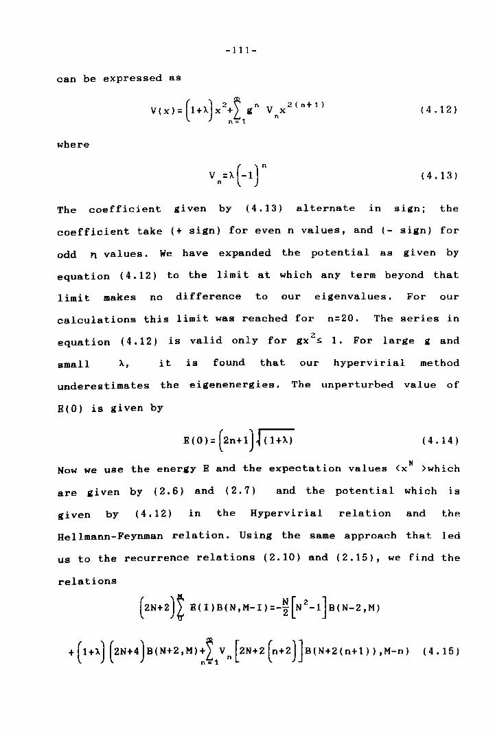
-111-
can be expressed as
( 4 .12 )
where
(4.13)
The coefficient given by (4.13) alternate in sign; the
coefficient take (+ sign) for even n values, and (- sign) for
odd t1 values. We have expanded the potential as given by
equation (4.12) to the limi t at which any term beyond that
limit makes no difference to our eigenvalues. For our
calculations this limit was reached for n=20. The series in
equation (4.12) z is valid only for gx ~ 1. For large g and
small A, it is found that our hypervirial method
underestimates the eigenenergies. The unperturbed value of
B(O) is given by
(4.14)
H Now we use the energy E and the expectation values <x >which
are given by (2 • 6 ) and (2 • 7 ) and the potential which is
given by (4.12) in the Hypervirial relation and the
Hellmann-Feynman relation. Using the same approach that led
us to the recurrence relations (2.10) and (2.15), we find the
relations
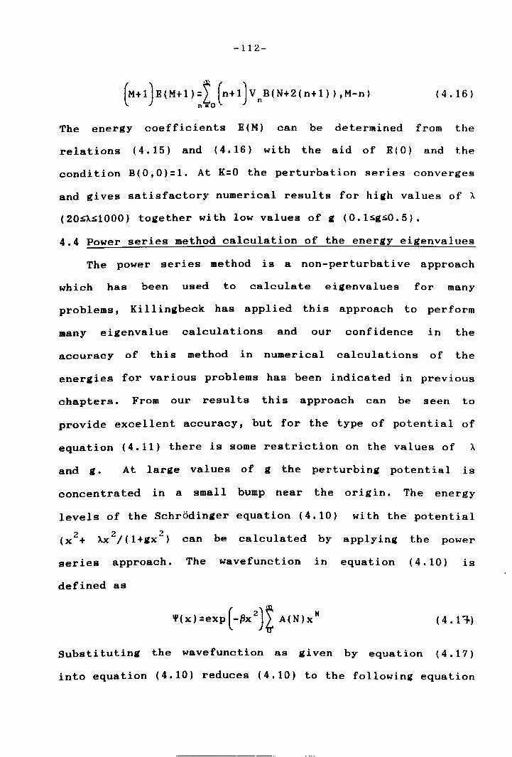
-112-
(4.16)
The energy coefficients E(M) can be determined from the
relations (4.15) and (4.16) with the aid of E(O) and the
condition B(O,O)=1. At K=O the perturbation series converges
and gives satisfactory numerical results for high values of A
(20s~1000) together with low values of g (0.lsgs0.5).
4.4 Power series method calculation of the energy eigenvalues
The power series method is a non-perturbative approach
which has been used to calculate eigenvalues for many
problems, Killingbeck has applied this approach to perform
many eigenvalue calculations and our confidence in the
accuracy of this method in numerical calculations of the
energies for various problems has been indicated in previous
chapters. From our resul ts this approach can be seen to
provide excellent accuracy, but for the type of potential of
equation (4.11) there is some restriction on the values of A
and g. At large values of g the perturbing potential is
concentrated in a small bump near the origin. The energy
levels of the Schr6dinger equation (4.10)
(x 2 + >..x 2 /(1+gx 2) can be calculated by
with the potential
applying the power
series approach. The wavefunction in equation (4.10) is
defined as
( 4 • 1 '1-)
Substi tuting the wavefunction as given by equation (4.17)
into equation (4.10) reduces (4.10) to the following equation
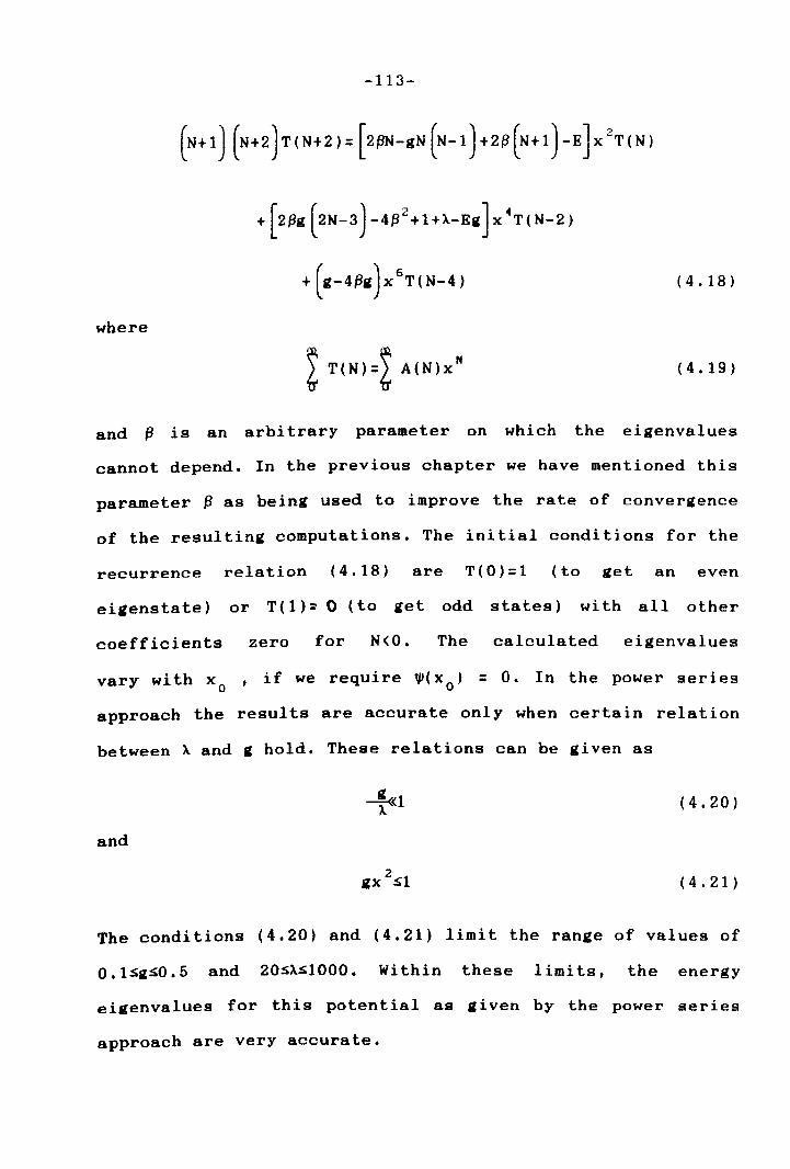
-113-
(4.18)
where
~ T(N)=~ A(N)x" (4.19)
and fJ is an arbitrary parameter on which the eigenvalues
cannot depend. In the previous chapter we have mentioned this
parameter fJ as being used to improve the rate of convergence
of the resulting computations. The initial conditions for the
recurrence relation (4.18) are T(O)=1 (to get an even
eigenstate) or T(1): 0 (to get odd states) with all other
coefficients zero for N<O. The calculated eigenvalues
vary with Xo ' if we require ~(xo) = O. In the power series
approach the results are accurate only when certain relation
between A and g hold. These relations can be given as
and
~<1 ).
2 gx :!O1
(4.20 )
(4.21)
The conditions (4.20) and (4.21) limit the range of values of
O.I~g~0.5 and 20:!OA~1000. Within these limits, the energy
eigenvalues for this potential as given by the power series
approach are very accurate.
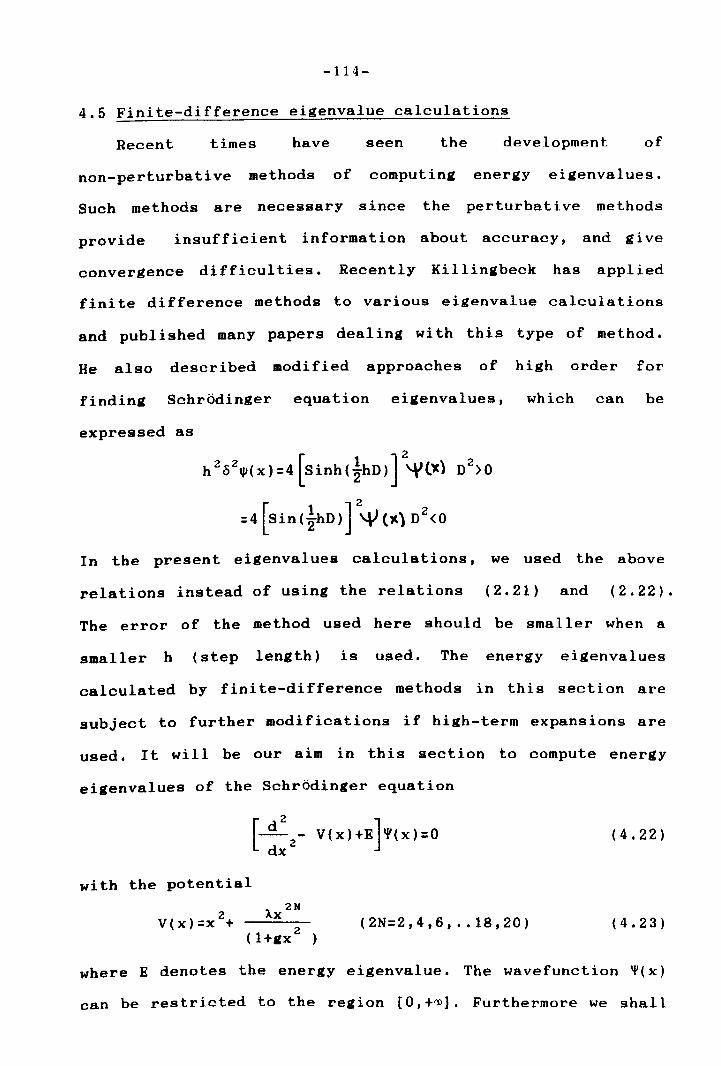
-114-
4.5 Finite-difference eigenvalue calculations
Recent times have seen the development of
non-perturbative methods of computing energy eigenvalues.
Such methods are necessary since the perturbative methods
provide insufficient information about accuracy, and give
convergence difficulties. Recently Killingbeck has applied
finite difference methods to various eigenvalue calculations
and published many papers dealing with this type of method.
He also described modified approaches of high order for
finding Schrodinger equation eigenvalues,
expressed as
h2021j1(X)=4[Sinh(ihD)]2'¥lX) D2)O
=4 [Sin (~hD) ] 2"" (1t) D2 <0
which can be
In the present eigenvalues calculations, we used the above
relations instead of using the relations (2.21) and (2.22).
The error of the method used here should be smaller when a
smaller h (step length) is used. The energy eigenvalues
calculated by fini te-difference methods in this section are
subject to further modifications if high-term expansions are
used. It will be our aim in this section to compute energy
eigenvalues of the Schrodinger equation
[_d2
- ] V(x)+E 1{I(x)=0 dx
2 ( 4 • 22 )
with the potential
'\ 2N 2 ",x
V(x)=x + (1+ax 2 (2N=2,4,6, .• 18,20) (4.23 )
where E denotes the energy eigenvalue. The wavefunction ~(x)
can be restricted to the region [O,+~]. Furthermore we shall
-115-
suppose that the wavefunctions are restricted to obey the
Dirichlet boundary condition ~(x)=O at some x value (x=R). An
acceptable R value will be guessed numerically. The interval
[O,R] is subdivided into equal parts of length h, with x=kh
(k=O,1,2, .• n; nh=R). The ground state and the first three
even energy levels were computed by our approach for a large
range of (A) and (g). In this section the finite difference
method for calculating eigenvalues of the Schrbdinger
equation (4.22) will be discussed by introducing a fini te
difference representation of n21J1(x). Chapter two explained
the simple mathematics which forms the basis of our method.
It is worth noting here that the finite difference method
which is under discussion in the present section is different
from that of the V.Fack and Vanden Berghe but it shares with
it the use of fini te di fference expressions. Those previous
workers used a finite difference method in combination with a
matrix diagonalisation for numerical computations and
transformed the Schrbdinger equation into an algebraic
eigenvalue problem, with a special form of matrix. A Finite
difference representation for DlJltx) is introduced such that
the Schrbdinger equation is transformed into an algebraic
eigenvalue problem. Our method gives results with high
accuracy for a wide range of 0 .1~g~lOOO and O. l:!>A:!>lOOO for
(2N=2,4,6 •• 18,20). For large g values it seems that the
present method works qui te well, whereas the other methods
have some problems. Although the displayed results are
restricted to even-parity states, the method can be used for
odd-parity states. We believe that the extrapolation
-116-
procedure (for h~) is very accurate if the h values are
chosen in the safe region.
4.6 The Pade approximant calculation of energy eigenvalues
We will now define the Pade approximant, and the Pade
table. Definition: Let the [L,M] Pade approximant to the
series A(x) be denoted by:
P L (x) [L,M]=--
QM(X)
where PL(x) is a Polynomial of degree at most Land Q M(X) a
polynomial of degree at most M. We require that the formal
power series for P/Q agrees with the A(x) series up to the
(L+M)th power. The following theorem is due to Frobenius.G.
and Pade, (Theorem of Uniqueness). The [L,M] Pade approximant
to any formal power series A(x), when it exists, is Unique.
(For the proof see ref [56,1975]. This theorem holds whether
the defining equations are non singular or not. If they are
non singular, then they can be solved directly to obtain:
a L -M+1 a L -M+ 1 a L + 1
a L a L+1 . . . a L +M
! XJ ! X J J~oaJ XJ a J-M a J -M+ 1 . . .
IsM ;=M-1 [L,M]=
a a a L-M+1 L-M+2 L+1
at a L+1 a L+M
XM X"-1 1
where we define a nB 0 if n<O; qj 5 0 if j > M and, if the
lower index on a sum exceeds the upper, the sum is replaced
-117-
by zero. It is customary to arrange the Pade approximants in
a table as follows:
[0,0]
[ 1 ,0)
[2,0}
[3,0]
[0, 1 ]
[1, l]
[2, 1 ]
[ 3 , 1 ]
[0,2]
[l ,2]
[2,2]
[ 3 , 2 ]
[0,3)
[ 1 ,3)
[2,3]
[3,3]
The set [N,O] [N,l] [N,2] with N fixed is a row of the table;
likewise the set [N,M] with M fixed is a 'column' while the
set [N,N] is the diagonal sequence; we call a set [N,N+j)
with j fixed, a paradiagonal. The top row is composed of the
partial sums of the Taylor series. The Pade approximants are
a particular type of rational fraction approximation to the
value of a function, Pade approximation is a useful technique
when the convergence of the series is unacceptably slow or
even nonexistent. The Pade approximant is in the form of one
polynomial divided by another polynomial. Pade approximants
provide us wi th a practical method of calculating resul ts
from energy series E (n) , since their use frequently
accelerates convergence. The E [M,N] Pade approximants to the
energy series is given by
a +a A + a A2+a A3 ••••• a A~ E [N,M]: __ a ___ 1 _______ 2 ____ ~3 __________ ~n~ __
b +b A + b A2+b A3 •••• b A~ o 1 2 3 M
(4.24)
2 H+N sE(0)+E(l)1+E(2)1 + ------E(N+M)l + --- (4.25)
with ba
defined to be unity. The coefficients (ai
i:l,-----N)
and (b,i:O,-----M)in the numerator and denominator are I
calculated from the knowledge of E( 1) ,E(2) ,-------,E(M+N),
which can be computed from the hypervirial relations. The
-118-
? ?
energy series for the interaction Ax~/(1+gx~) appears to be
convergent for g> 5 and for large value of A. Thus we can
still calculate the energy E for g>5 to very high accuracy. n
Our calculated energy values E used the n
[6,6] Pade
approximants to the energy series for the ground and the
first three excited states.
4.7 Hypervirial relations for the potential given by
[1 2 2N 2 ] 2x -gx /(l+gax) (2N=4,6)
In this section, we want to investigate
equation
[i ::2 + E-V(X)]~(X)=O with a potential of the type
2 2" V~=~ ~ --~g~X----2
(1+gax ) (2N =4,6)
the Schrodinger
(4.26)
(4.27 )
The potential described by equation (4.27) for (2N=4) has
recently been studied by G.Auberson (30,1982], who has shown
that the perturbation expansion of eigenvalues E in terms of
g at fixed a, is Borel summable. For the validi ty of this
results, it is essential that the potential V(x;g) be
positive for all physical values of g and a, where the
physical range of the parameters (g and a) is given as; for
the potential V+(x;g),g~O, a)O, and for V-(x;g),g~O, a>2, (in
2 order that V-(x,g)~, as x ~).
Also G.Auberson and T.Boissiere [31,1983] calculated ground
state energy levels for a large range of values of a and g,
by using a Pade method, Borel-Pade method, an improved
Borel-Pade method and Borel-mapping method). The potential
-119-
V~ (x,g) can be written in this form 2N
We want to study the limit of this potential
~ I 1 2 2M V (x;i) =2X + iX IX .. 0
(2N=4,6)
(4.28)
(4.29)
(4.30)
The potential given by equation (4.30) is a pure anharmonic
oscillator The singularity of V+(x;g) at 2 x = is
responsible for a singularity of E+(g) and for the divergence
of the potential series expansion. We investigate three
methods to compute the energy eigenvalues, the hypervirial
method, the Pade approximants method and the finite
difference method. The first two methods are excellent for
computing the energy for a small range of values of IX and g ,
but the finite difference approach is applied to a wide range
of values of IX and g. In this section, we apply the
hypervirial theorem and the Hellmann-Feynman theorem to
calculate the eigenvalues of the Schrodinger equation for
this potential. The potential V+(x) can be expanded as
where the potential coefficient V is n
and
( 4 .31 )
-120-
A=gex (4.33)
The unperturbed energy eigenvalue E(O) is given by
11= 1 +AK (4.34 )
If we insert the energy (E) series and the expectation value
<x N ) series in the hypervirial relation, the following
relation is obtained
(2N+2)! E(I)B(N,M-I)=-~[NZ-1]B(N-2,M)
+ (N + 2) [1lB ( N + 2 , M ) - KB ( N + 2 , M - 1 ) ]
If we apply the Hellmann-Feynman theorem
the following relation is obtained
(4.35)
(4.36)
(4.37)
We can calculate the energy eigenvalues from equations (4.3S)
and (4.37) by using the unperturbed energy E (0) and the
ini tial coefficient value B (0,0) = 1. We also used the same
technique with g as the perturbation parameter. The agreement
between the re suI ts from the two approaches is excellent,
particularly for low value of ex, but at high values of ex the
agreement between the two eigenvalues decreases, and this is
very clear from our results in table (4.10 ). The potential
-121-
V+(x) in equation (4.27) can be expanded in the form
(4.38)
where
V n = (-ex) n, 11= 1 + Ak (4.39)
The coefficients given by equation (4.39) alternate in sign,
taking positive and negative values for even and odd powers
respectively. If we follow the same procedure used to get the
relations (4. 3S) and relation (4.37), we get the following
relations
+ (N + 2 ) [IJB ( N + 2 , M ) - KB ( N + 2 , M - 1 ) ]
(4.40)
(4.41)
The above equation (4.40) and (4.41), together with initial
conditions E(O)=
sufficient to
1 2 [2n+1].fji
compute the
(n=0,1,2) and B(0,0)=1 are
coefficients E(M) of the
perturbation series for the energy. The method outlined above
can also be used for the potential which is given by equation
(4.29). For high-index (2N=4, 6 ) perturbation calculation by
the hypervirial method, the method seems to work only for
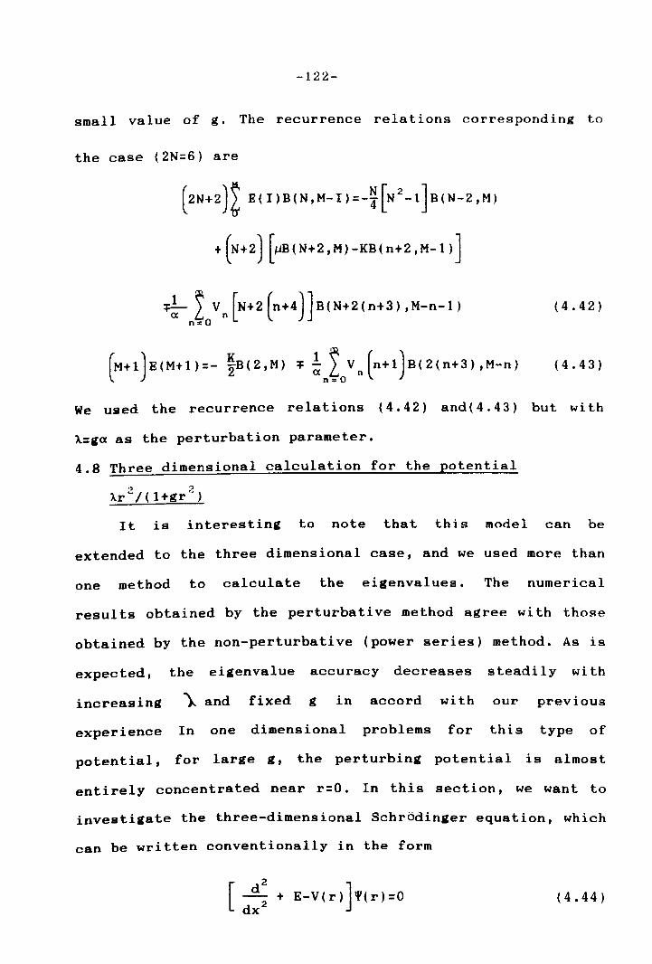
-122-
small value of g. The recurrence relations corresponding to
the case (2N=6) are
(2N+2)~ E(I)B(N,M-I)=-~[N2_1JB(N-2,M)
+ (N + 2) [1lB ( N + 2 , M ) - KB ( n + 2 , M - 1 ) ]
(4.42)
(4.43)
We used the recurrence relations (4.42) and( 4.43) but wi th
X=ga as the perturbation parameter.
4.8 Three dimensional calculation for the potential 2 . .,
).r /(l+gr~)
It is interesting to note that this model can be
extended to the three dimensional case, and we used more than
one method to calculate the eigenvalues. The numerical
results obtained by the perturbative method agree with those
obtained by the non-perturbative (power series) method. As is
expected, the eigenvalue accuracy decreases steadily with
increasing ~ and fixed g in accord with our previous
experience In one dimensional problems for this type of
potential, for large g, the perturbing potential is almost
entirely concentrated near r=O. In this section, we want to
investigate the three-dimensional Schrodinger equation, which
can be written conventionally in the form
(4.44)
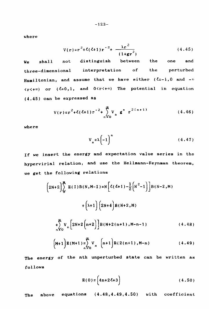
-123-
where
2 g g -2 V(r):r +~(~+1)r + (4.45)
We shall not distinguish the one and
three-dimensional interpretation of the perturbed
Hamil tonian, and assume that we have either (t:-1, 0 and _.\)
<r<+~) or (.(.:0,1, and O<r<+~) The potential in equation
(4.45) can be expressed as
V(r):r 2 +'('(.(.+1)r- 2 + 2 Vn in n .. O
where
2(n+1) r (4.46 )
(4.47 )
If we insert the energy and expectation value series in the
hypervirial relation, and use the Hellmann-Feynman theorem,
we get the following relations
(2 N + 2 ) ~ E ( I ) B ( N , M-I ) : N [ t ( i+ 1 ) -~ ( N 2 - 1 ) ] B ( N - 2 , M )
+~ Vn [2N+2(n+2)]B(N+2(n+1),M-n-l) n=O
(4.48)
(4.49)
The energy of the nth unperturbed state can be written as
follows
E ( 0 ) : ( 4 n + 2 i+ 3 ) (4.50)
The above equations (4.48,4.49,4.50) with coefficient
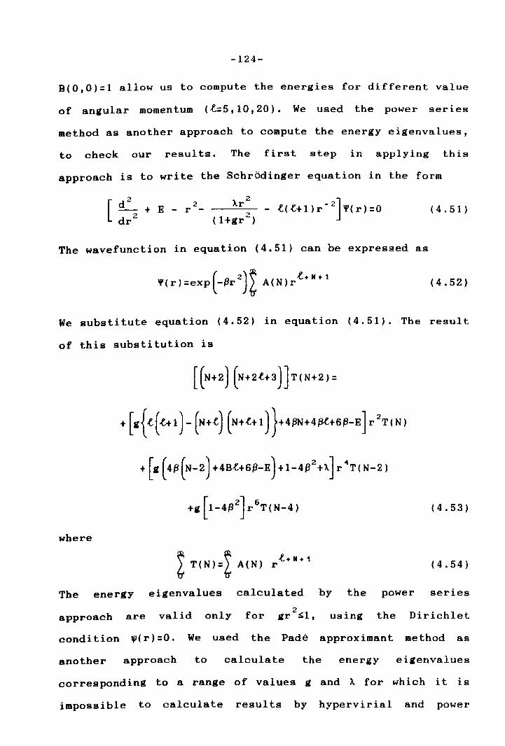
-124-
B(0,0)=1 allow us to compute the energies for different value
of angular momentum (t=5, 10,20). We used the power ser ies
method as another approach to compute the energy eigenvalues,
to check our results. The first step in applying this
approach is to write the Schrodinger equation in the form
+ E -2
r - ( 4 . 51)
The wavefunction in equation (4.51) can be expressed as
(4.52)
We substitute equation (4.52) in equation (4.51). The result
of this substitution is
+ [g (4fJ (N-2) +4Bt+6fJ-E) + 1-4fJ2 +".J r 4T (N-2)
(4.53)
where
~ T(N)=~ A(N) (4.54)
The energy eigenvalues calculated by the power series
approach are valid only for 2 gr ~1, using the Dirichlet
condi tion 1P( r) =0. We used the Pade approximant method as
another approach to calculate the energy eigenvalues
corresponding to a range of values g and A for which it is
impossible to calculate results by hypervirial and power
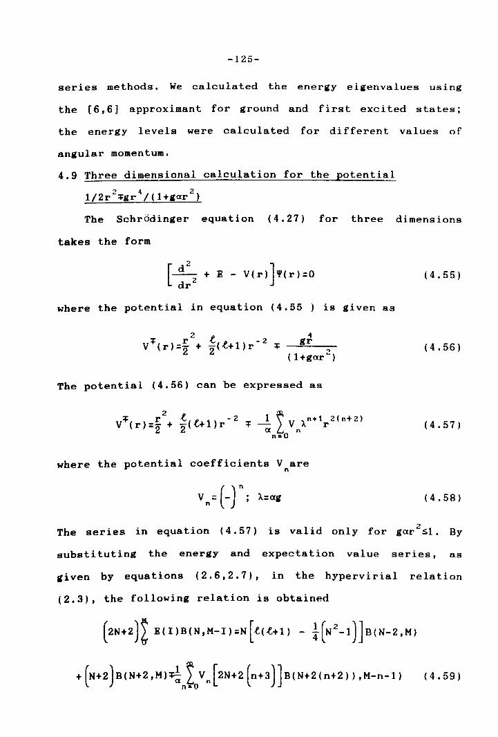
-125-
series methods. We calculated the energy eigenvalues using
the [6,6] approximant for ground and first excited states;
the energy levels were calculated for different values of
angular momentum.
4.9 Three dimensional calculation for the potential
.., 4 2 1/2r~~gr /(1+gar )
The Schrodinger equation (4.27) for three dimensions
takes the form
where the potential in equation (4.55 ) is given as
2 4 + r .t ~ - 2 gr V (r)=2 + 2(~+1)r ~ 2
(1+gexr )
The potential (4.56) can be expressed as
+ ) r2 t( ~ 1) -2 or _1 ~ V ,\n+1 r 2(n+2) V (r =2 + 2 '\..+ r or ex L n A
n=O
where the potential coefficients V are n
V n = (_ ) n; A:exg
(4.55)
(4.56 )
(4.57)
(4.58)
The series in equation (4.57) 2 is valid only for gexr ::;1. By
substituting the energy and expectation value series, as
given by equations (2.6,2.7), in the hypervirial relation
(2.3), the following relation is obtained
(4.59)
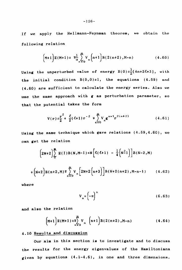
-126-
If we apply the Hellmann-Feynman theorem, we obtain the
following relation
1 Using the unperturbed value of energy E (0) =2"[ 4n+2{+3], wi th
the initial condition B(0,0)=1, the equations (4.59) and
(4.60) are sufficient to calculate the energy series. Also we
use the same approach wi th g as perturbation parameter, so
that the potential takes the form
v (r) =~ \ ~(.t+ 1) r - 2 + ~ V ng n+ 1r 2 (n+ 2)
n=O (4.61)
Using the same technique which gave relations (4.59,4.60), we
can get the relation
(4.62)
where
(6.63)
and also the relation
(4.64)
4.10 Results and discussion
Our aim in this section is to investigate and to discuss
the results for the energy eigenvalues of the Hamiltonians
given by equations (4.1-4.6), in one and three dimensions.
-127-
Our aim also is to push the numerical analysis as far as
possible, and in this respect we go further than other people
in our analysis. We study here the three dimensional problem
and high indices 2N of the perturbation. In addition we have
succeeded in finding the energy eigenvalues wi th excellent
accuracy. This problem received great attention from us , and
we have attacked it by many methods, as we mentioned in a
previous section. In summary, we have analysed numerically
four different methods to determine the energy eiatenvalues
for these problems for different values of state number nand
a wide range of values of (A&g) and indices (2N:2,4, •. 18,20).
The finite difference method has been used for calculations
outside the limits applicable to the other three methods
(hypervirial, Pade approximant and power series),
particularly in respect to the values of parameters (g&A) and
of the index of the perturbation (2N:2,4,6, .•. 18,20). It is
note worthy that the methods which have been applied to
compute our results are applicable within a limited range of
(2N,A,g), except for the finite difference method, which
seems to present fewer difficulties. We have used the
hypervirial method to calculate results for various model
problems, such as those given by (4.1,4.2,4.3,4.4,4.5,4.6),
for different values of (2N,A,g,n). The present work is
intended to point out one feature which has not been noted in
previous problems. The hypervirial method can produce a good
accuracy even without use of the renormalisation parameter K,
which usually plays an important role in obtaining convergent
perturbation series, as we have seen in previous chapters. We
-128-
have performed a series of computations for the problems of
this chapter, which revealed the following fact. As the index
(2N) increases the sums of the perturbation series converge
very well for small values of A, and as A increases the
convergence begin to decrease. If we review briefly our
listed results in tables (4.3,4.7,4.10,4.12 ,4.13), we can
get a clear picture of this behaviour. We can say that the
accuracy of our listed results is very good in comparison
wi th other resul ts which are available in the literature.
Also the results which are produced by the hypervirial method
are in good agreement with our results which have been
calculated by the power series and finite difference methods.
This agreement provides a check on the accuracy of our
results. We have computed the first four energy eigenvalues
for index (2N=2), with parameter values 5 O!S.A!S. 1 000 ,
0.1!S.g!S.0.50, by using three methods (hypervirial, power series
and finite difference). The accuracy of our results in
general is more than 16 significant digits, as shown in
tables (4.1,4.2). The power series method seems to work very
well and the convergence of this method will be controlled by
the parameter ~. We also listed in table (4.4) the four first
energy eigenvalues for (2N=2) and for values O. 2!;g!S.50 and
500~~106, obtained by using Pade approximants [6,6] and the
hypervirial method. The agreement between the two methods is
very good. Also we have calculated the first five energy
levels by using the hypervirial method for (2N=4), with case
V-(x) for 10-3!S.g~0.02; 1~!S.50. In addition we used Pade
approximants for (O.1!S.g~2; 2~!S.50). We have observed a strong
-129-
similarity between the behaviour of the hypervirial method in
one and three dimensional calculations for changing index of
perturbation (2N) and value of (g&A). The series converge
very quickly for large A and small g with (2N=2), but with
(2N:4,6) the si tuation is not similar; the series converges
for small values of A and larger values of g. Further more it
clearly appeared from our listed results in tables
(4.12,4.14), that the perturbation calculations (Hypervirial
calculations) can yield very high accuracy for large values
of a, if we take ag as perturbation parameter in stead of g.
For small values of a,it does not make any different to the
accuracy whether we take ag or g as perturbation parameter.
Also we have not observed any fundamental difference in
behaviour between the V-and V·cases as we vary the
perturbation parameters (a,g) and index (2N=4,6). We have
calculated the first five energy eigenvalues in three
dimensions for di fferent sets of A, g, index (2N=2, 4,6) and
angular momentum. It is note worthy that the Pade approximant
method [M, N] has been applied to this problem for one and
three dimension and is able to handle this problem over a
wide range of O. 1~g~50 j 6 O. 1~A~10 , and index power
(2N:2,4,6). Some of the present calculations of eigenvalues
have been repeated with two different values of N and M in
order to check the accuracy, since there is an absence of
reported results in the literature. The agreement between the
two eigenvalues is very good. We wish to draw attention to
the fact that the present Pade approximant approach works
very well even for higher values of (g,A), whereas the Pade
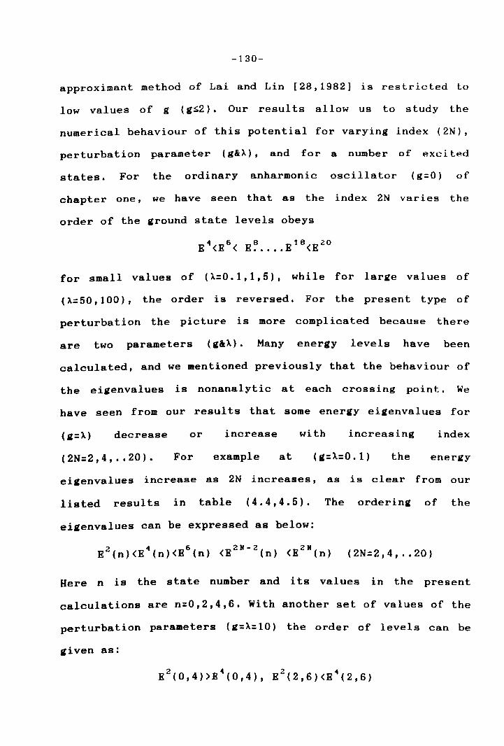
-130-
approximant method of Lai and Lin [28,1982] is restricted to
low values of g (g~2). Our results allow us to study the
numerical behaviour of this potential for varying index (2N),
perturbation parameter (g&).), and for a number of exci ted
states. For the ordinary anharmonic oscillator (g=O) of
chapter one, we have seen that as the index 2N varies the
order of the ground state levels obeys
E4
<E6
< E? ••• E16
<E20
for small values of (A=0.1, 1,5), while for large values of
().=50, 100), the order is reversed. For the present type of
perturbation the picture is more complicated because there
are two parameters (g&X). Many energy levels have been
calculated, and we mentioned previously that the behaviour of
the eigenvalues is nonanalytic at each crossing point. We
have seen from our results that some energy eigenvalues for
( g=).) decrease or increase with increasing index
(2N=2,4, •• 20). For example at ( g= A=O . 1 ) the energy
eigenvalues increase as 2N increases, as is clear from our
listed results in table (4.4,4.5). The ordering of the
eigenvalues can be expressed as below:
(2N=2,4, .• 20)
Here n is the state number and its values in the present
calculations are n=O,2,4,6. With another set of values of the
perturbation parameters (g=X=10) the order of levels can be
given as:
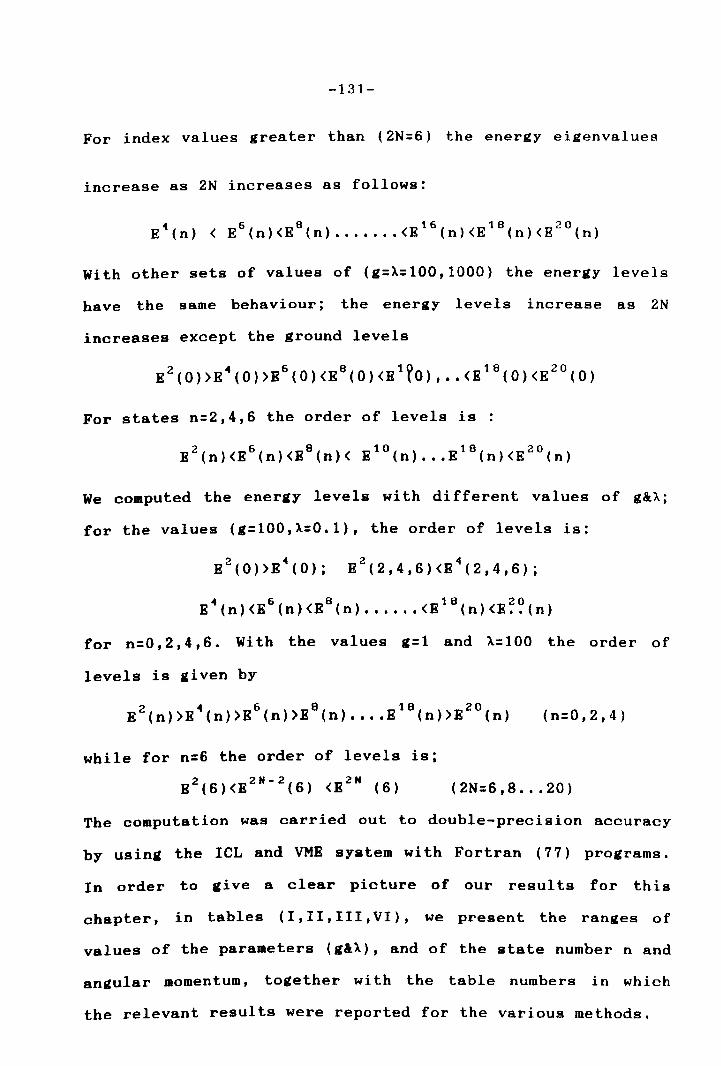
-131-
For index values greater than (2N:6) the energy eigenvalues
increase as 2N increases as follows:
With other sets of values of (g:A:IOO,lOOO) the energy levels
have the same behaviour; the energy levels increase as 2N
increases except the ground levels
For states n:2,4,6 the order of levels is :
We computed the energy levels with different values of g&A;
for the values (g:100,A:0.1), the order of levels is:
2 4 E (2,4,6)<E (2,4,6);
4 6 8 18 20 E (n)<& (n)<E (n) •••••• <E (n)<& •. (n)
for n=0,2,4,6. With the values g=1 and A=100 the order of
levels is given by
2 4 6 8 18 20 E (npE (npE (npE (n) •••• E (n»E (n) (n:0,2,4)
while for n=6 the order of levels is;
E 2 (6)<E2N
-2
(6) <E2N
(6) (2N=6,8 .•• 20)
The computation was carried out to double-precision accuracy
by using the ICL and VME system with Fortran (77) programs.
In order to give a clear picture of our results for thi s
chapter, in tables (I,II,III,VI), we present the ranges of
values of the parameters (g&A), and of the state number nand
angular momentum, together wi th the table numbers in which
the relevant results were reported for the various methods.
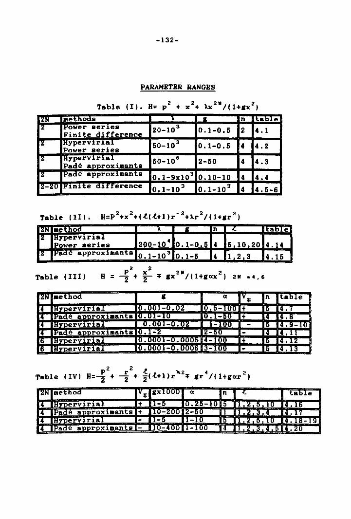
-132-
PARAHBTBR RANGBS
iZN aethoCls 1-
----n l!-ab~e
12 IPower aerl.es 20-10 3 0.1-0.5 2 4.1 Finite difference ~. IHypervl.rl.al 60-10 3 0.1-0.6 4 4.2 Power aeries 12 IHypervl.rl.al 50-106 2-50 4 4.3 Pade approxiaants 12 [Pade apprOXl.mants 0.1-9xl0 3 0.10-10 4 4.4 IZ-~O IF l.nl. te Cll.l't-erence 0.1-10 3 0.1-10 3 4 4.5-6
Table (11). 2 2 -2 2 2 H=P +X +(~(~+l)r +lr 1(1+,r )
IZN method ~ • n <. Ita~e
12 IHypervl.rl.aJ. 200-10 4
Power aeriea 0.1-0.6 4 6 J lO...l.20 4.14 12 IPaCle apprOX1aanta 0.1-10 3 0.1-6 4 1, 2.3 4.15
Table (Ill) P
2 x2 211 2 H = ~ + ~ ~.X l(l+.ax) 211 a.,6
12N aethod I a IV~ n IT.aDle
14 HyperVl.r1al 10.Ot I!-J!.~Z jJ. fi- lOO + I'.~
Pade aooroX1aants 0.0 -10 Q.~-- )0 + I •• IS iYDerv1r1al O. }llJI-O.OZ 1- ~O - • -J,JL
14 PaCl e aJ)P.rox 1.man ts O. 1-~ :l- - L' • If IYDerV1r1.aJ. O. ()Olli -..Q.. 0005_ 4- IU + L' •
It IYDerv1r1al O. ()Q(U -0.0006 3- IU - J:t ~.
12N aethoCl V~ IrxIUUO a n -t. T.aD~e
IHyperv1r1al + -5 IL. -.ID ) t t ...l.. J!. ~.1..6 IPade aoorOx1mants + lO-:lOO - ~ • t ·ll IHYDerV1r1al - -5 - ) _f • .U .11S-il
rl· IPade aDPrOx1mants - .Q-.400 - ~o . .1 • J .5 • :lJ!.
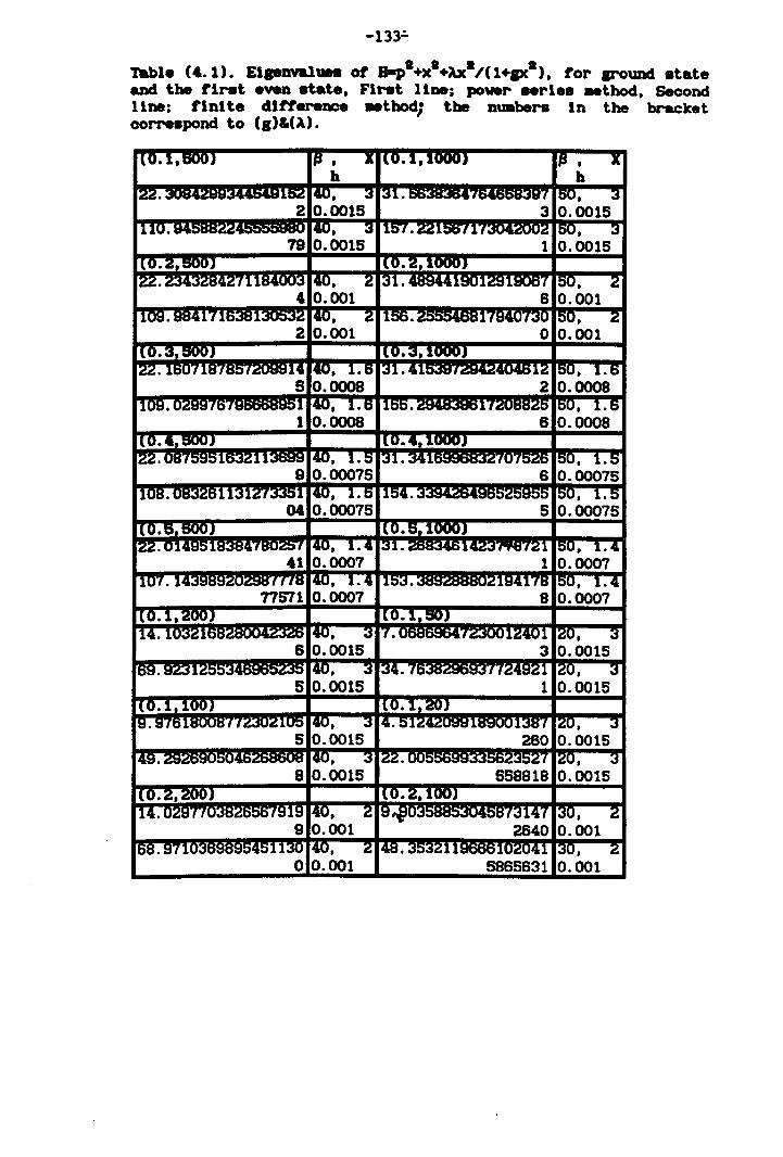
-133';'
Table ('.1). ElaeDYalue. of ~·+X·+Ax·/(l+IX·), tor around .tate anc:l the tlrllt ev.n .tate, Flrllt 11 .. ; power .erle. _thod, Second line: tlnlte dlfterenoe .. tbod; the nuabers In the bracket oorreapond to (I)&(A).
, , o 0.001 5865631 0.001
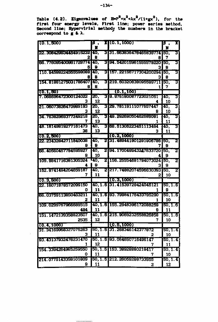
-134-
Table (4.2). Elaenvalun ot S-pl+XI+AxI/(1+pl), for the tiNt tour "raY level., FINt line; power .erles _thod, Second. llnei Jbfpervlrlal .tbodJ the nuabera In the bracket correspond. to • & A.
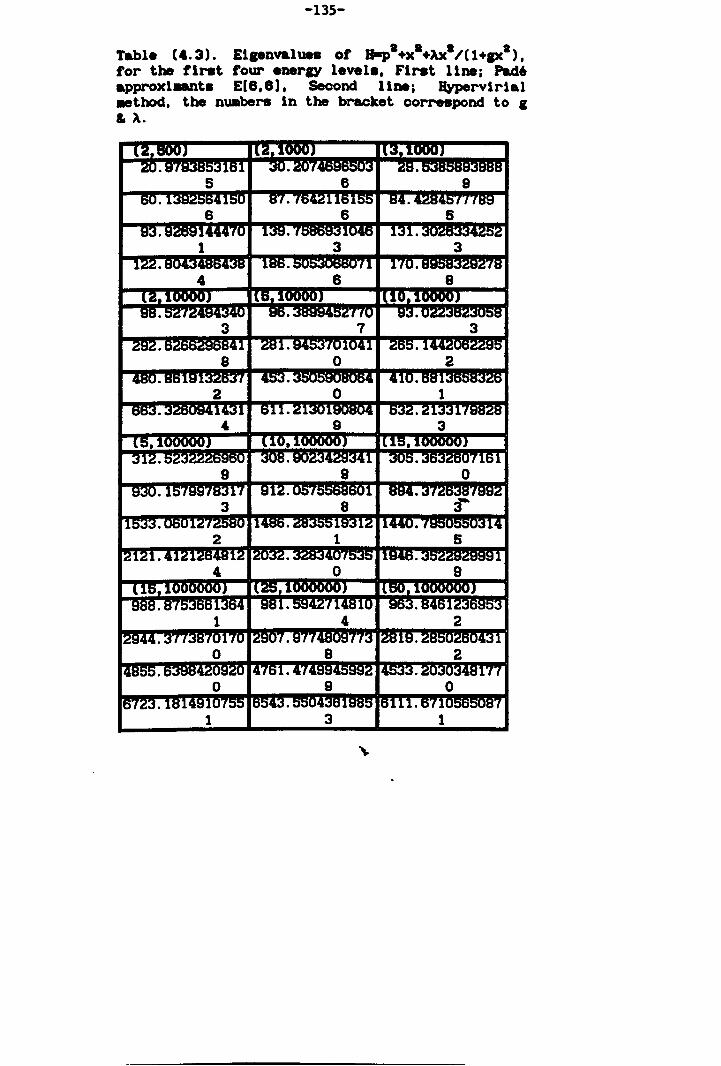
-135-
Table (t.3). El.envalue8 of s-p8+X8+Ax8/U +p l). for the tlr.t tour enarlY levela, Flr.t Una; Pad, approxl-.nta E(8,8), Second 11ne; Jbrpervlrlal _tbod, the nuabers in the bracket correspond to I & A.
1 3 1
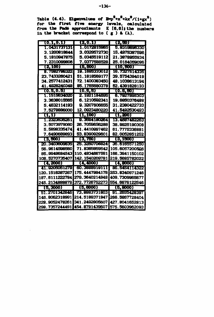
-136-
Table (4.4). El....-1-- or a-p1+xl+lxl"(1+pl) tor the I'lrst 1'1". eDer8Y 1.".1.. calculated troa tbI ..... .,..-oxl.ant. E [8.8h the nwabera In the llracbt corN8pODd to ( • ) & (A).
3.363801S58S 5.4632114193 7. 5278886000
3. 50739'79060 5. 5898335t74 7. 8490689893
.
39. S7St394019 48.1038613194 52.&391828133
146.8062318991 214.5189371947 266.5867728404 228.9052478281 341.2G280S607 427.8041852813 298.73572«491 454.8791439807 575.5603982093
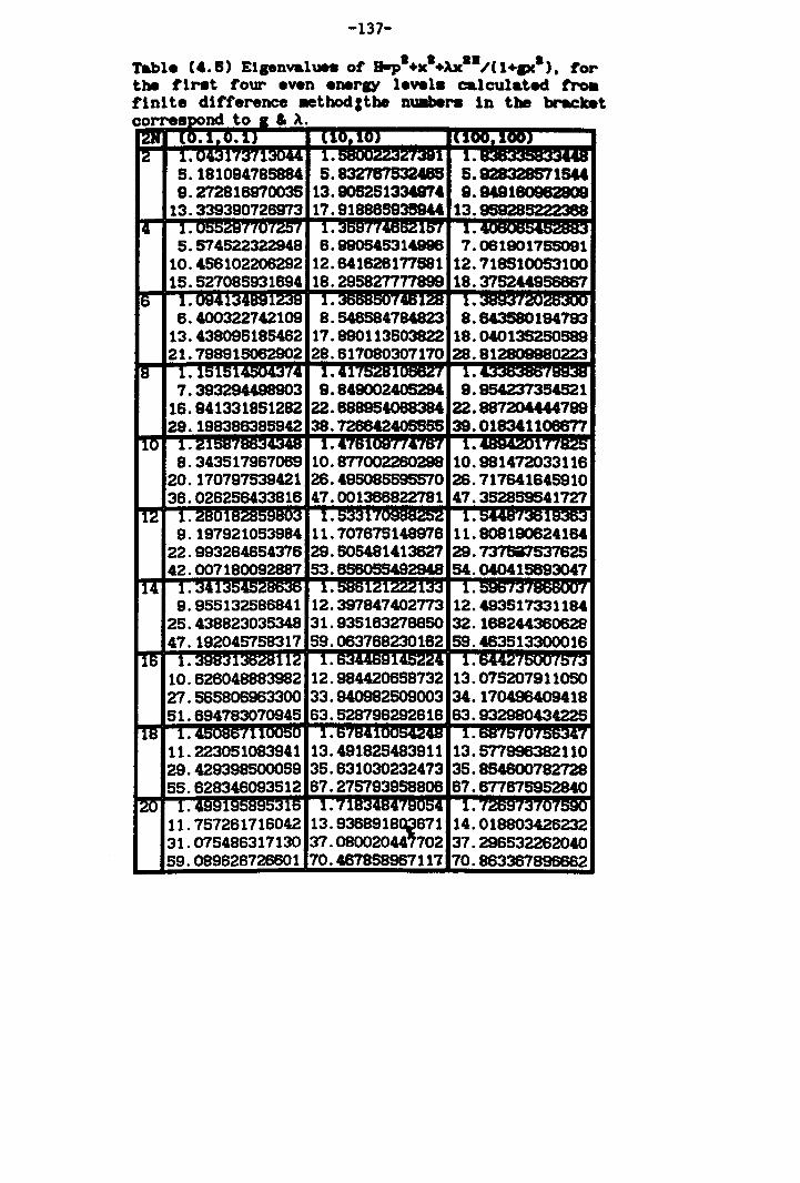
-137-
Table (4.6) Elpnvalue. ot a-p·+X·+Ax··/U+p·). tor the tl,..t tour even enerD' level. calculatttd troll flnlte dlfference _tbod:tbe nuaber. in the bracket corres Dd to & A.
11.757261716042 13.9368918~671 14.018803426232 31.075486317130 37.08002044'702 37.296532262040 59.089626726601 70.467858967111 70.863367896662
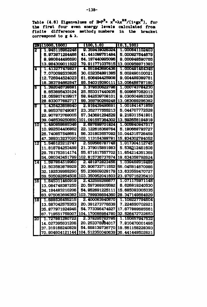
-138-
Table (4.8) Ei.envalues of B-pa+ xa+Axs ·/(I+axa ). tor the tirat tour even enerD' levels calculated troll tlnite difference _thod, nuabera in the bracket correspond to • & A.
.
25.553317440935 58.942539708101 99.359790289248
14.027395631206 20.253378 4017 7.810470001495 37.319188240829 54.868139736710 19.561158228393 70.904604121144 104.512350040639 36.441449502621
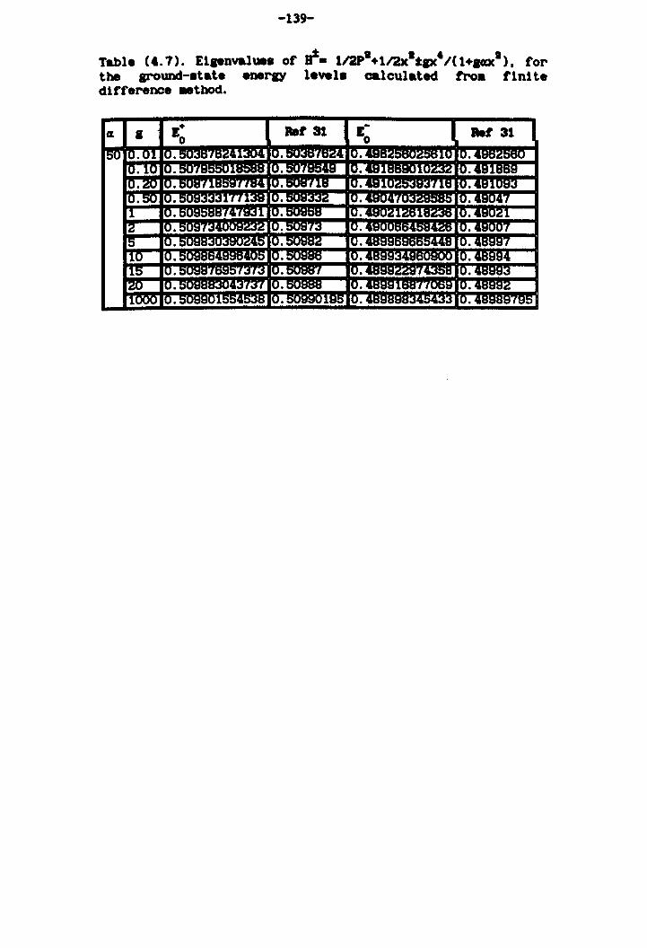
-139-
Table (&.7). Elaenvalues ot at. 1I2Pa+1I2xatIX1 /(1+aaxa), tor the around-.tate ener8)' level. calculated fro. tinl te dlfference _thod.
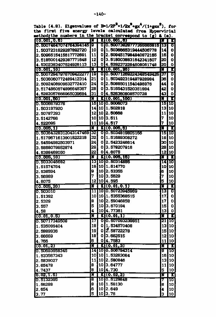
-140-
Table C4. 8). Eipnvalues of 1fa1l2pa+1I2xa+p'IC l+.cxxa ), for the fiM1t five enerlY level. calculated fro. Jb'pervirial -tbod the wabe 1 the b k t C ) 11 n re n rac e COrretlJ)OM to Ca) & It. 1(0.001.0.I:IJ IN ~ I(O.OOl.aJ 'N 11: 10. t)UU1..v.IUI·IIII ~145 18 0 10. awl.JtSaJ111 fR 113 --u 1.5037231829287892720 10 0 1.503888S319U4S06778 14 0 2.5096515415817772891 11 0 2.6084517984940872185 18 0 3.5185001429387771848 12 0 3.5180038831842341807 20 0 4.5302383407624926113 13 0 4.5292372284608061748 20 0 [(0.001,10) IN It 1(0.001.20) IR -.: 10. DUuf~'(I:HtH :11 118 0 10. :;007' 137 0 1.5036060772489412314 21 0 1.503492319497928984 36 0 2.5092408909632772410 24 0 2.50885011540498976 " 0 3.5174860974896648367 28 0 3.5165431520351994 42 0 4.5282057666965039694 31 0 4.526360808570728 43 0 (0.001.aoJ IN ~ (0.001.100) IN -.: o. i-,t:I~-'1:) 115 ,10 o. ,.H~ 115
110
1. 503197920 14 10 1.602818 13 10 2.50787393 12 10 2.50668 11 10 3.5142766 10 10 3.511 7 10 4.522095 11 10 4.517 7 10 (0.0Uti.11 IN ~ (0.005.6) IN I: 0.~~R1L~7R~lZ043147469 13Z 0 .0.-.:;n~19805166 115 110 1.5179671613901822218 32 0 1.51689308272 16 10 2.54594982503971 24 0 2.5423246614 30 10 3.5968079952874 29 0 3.578207918 28 10 4.6398468050 22 0 4.6075 12 10 {0.OO5.10) IN I: (O.OO5.UU IN I: O. 113 10 0.50314886 114 110-1.51574764 19 10 1.514770 10 10 2.538594 9 10 2.53355 6 10 3.56969 7 10 3.5829 7 10 4.6075 12 10 4.595 5 10 (0.OO~20) IN I: (0.01.0.1) IN -X 0.:lU~U10 111 10 O.DUI C [I3 1r 1.51392 10 10 1.5355388515 17 0 2.5329 8 10 2.59046858 17 0 3.657 5 10 3.670194 15 0 4.58 4 10 4.77361 13 0 1(0.01,0.5) IN It 1(0.01.1) III IC 10. 50717~4Q ... nR 117 0 10.oU-( i1 121 110 1.535099404 18 0 1.534570408 13 10 2.5889936 19 0 ~.58722278 15 10 3.66669 18 0 3.66?S15 12 10 4.766 6 0 4.7593 11 10 1(0.01, Z) IN It 1(0.01,3) IN -.: 10. t4R 114 110 10. :wol94314 18 i10 1.533567343 10 10 1.53263064 16 10 2.5839027 11 10 2.580846 13 10 3.65478 8 10 3.64777 11 10 4.7437 8 10 4.730 5 10 rO. OZ,I.5) IN It ,(0. OZ, Z) IN IC 10. 51 18 110 ,0.5'?QR~ 17 10 1.56288 8 10 1.56130 8 10 2.654 6 10 2.649 4 10 3.77 5 10 3.76 3 10
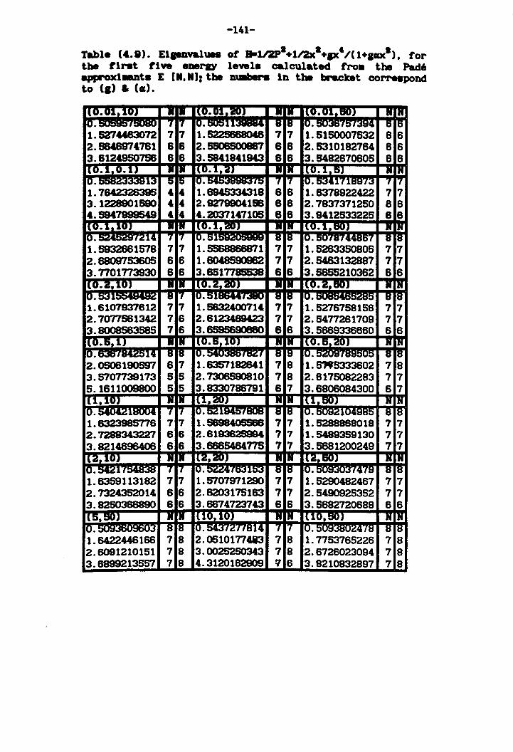
-141-
table ('.8). El~ues of B-112P1+112x1 +1X1/(1+.axl ), for the tlrst tl.. eaer8V le .. l. calculated fro. the Pad, approxlaant. E lR,Rl: the nu.bera In the bracket COrN_pond to (a) & (a).
1(0.01,101 • - IlO.Ul,iSUl 11 III IlQ.Ol,6OJ 11 N 10. I/:K.RSU 7 7 IU.50511~ II III IU. ou.JO,;,'3tfIJ. 6 6 1. 627.&463072 7 7 1. 522S8680t8 7 7 1. 6160007632 8 6 2.684697'781 6 6 2. 5S08SOO887 6 8 2.5310182784 6 6 3.6124950756 6 6 3.5841841943 6 6 3.6482670605 6 6 IlO.l,V.1) .. .. 1(0.1.2J R IR IlV.l,5J N N 10. 113 5 5 IU.-.J .,;, 7 7 10. 5341'flS~:rr3 "f "f
1. 7642326395 4 4 1. 8945334318 6 6 1.6378922422 7 7 3.1228901590 4 4 2. 92'79904156 8 8 2.7837371260 6 6 4.5947999549 4 4 4.2037147105 6 8 3.9412533225 8 8 !(0.1,-~ R I. IlV.l, iSUJ 11 I. IlO.l,80J • IN IU. ".:: 14 7 17 10.51 8 18 10. ;JUla,_OI 8 IB 1.5932661578 7 7 1. SS68888871 7 7 1.6263350805 7 7 2.6809753605 6 6 1.6048590962 7 7 2.5483132887 7 7 3.7701773930 6 6 3.6517785538 6 6 3.6656210362 6 6 {0.2.10J -I· l~.~,iSUJ .11 I- IlO.2,6OJ .. IN 0.5;31 II 17 0.51 ,r.sIJU II III IU. I'M i:i'!"h 8 18 1.6107937612 7 7 1.5832400714 7 7 1. 5276758156 7 7 2. 7077661342 7 6 2.6123489423 7 7 2.5477261709 7 7 3.8008663585 7 6 3.6595690660 8 6 3.5669336660 6 6 (0.5,1) -I- lV.5,lVJ N IN IlO.5,~OJ 11 IN 0.D.JO,~14 B IS U. 110£1 B IS lu.o~wl 8 18 2. 0S06190S97 6 7 1.8357182641 7 8 1. 679'6333602 7 8 3.5707739173 5 5 2.7306590810 7 8 2.8175082283 7 7 5. 1611009800 5 5 3.8330786791 6 7 3.6806084300 6 7 (1.10J N iN lJ..~J 11 III Ill,5OJ _N IN O. IiUIJ 1.&7, It1UU4 7 :7 O. 5Z 1845"ftsUtS 8 18 IU. f;U8~: I.4.QR'" 8 18 1.6323985776 7 7 1.5698405566 7 7 1.5288968018 7 7 2. 7288343227 6 6 2.6193625994 7 7 1.6489359130 7 7 3.8214696406 6 6 3.66854M77S 7 7 3.5681200249 7 7 (2,10J 11 11 (2.2OJ 11 IN 1(2,60) N IN IO.~H: 7 7 0.5ZZ4763153 8 18 10. il,,"rS 8 18 1.6359113182 7 7 1.5707971290 7 7 1.5290482467 7 7 2. 73243S2014 6 6 2.6203175163 7 7 2.5490925352 7 7 3.8250366890 6 6 3.6674723743 6 6 3.5682720688 6 6 I(S,50} 11 11 (10,10) 11 III IllO,5OJ I! LN 10. B B U. 54J'I~1 ,a14 ., I-r 10. 1~47B 8 IB 1. 6422446166 7 8 2.0510177483 7 8 1.7753765226 7 8 2.6091210151 7 8 3. 0025250343 7 8 2.6726023094 7 8 3.6899213557 7 8 4.3120162909 ~ 6 3.8210832897 7 8
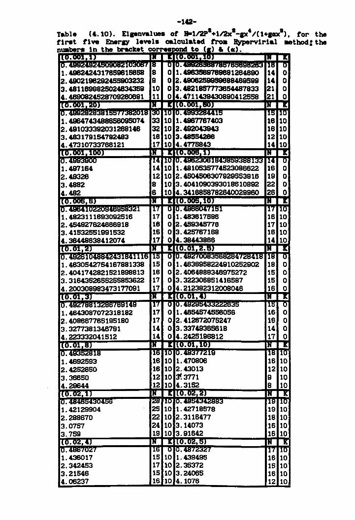
-lG-
Table (C. 10). Elpnvaluea of a-112P1 +112x1-p·/( l+.crxl ). for the flnt flve Enerl)' level. calculated tro. Jb'pervlrla1 _tbocl: the nuaben in the bracket corretl)ODd to (a) & (a). IlU.UU1,l) I. ~ I(U.OU1.1U) I. --.: 10 . :lU"'-'D1 18 0 10. "DOl 116 0 1. G62424317859816868 8 0 1. G83589789881284890 14 0 2. 49021982924S5903232 9 0 2.4908259989888489599 14 0 3. 4811899826024834359 10 0 3.4821857773854481833 21 0 4.4880824528709280891 11 0 4.4111438430890412568 21 0 1t0.OU1,20) lit --.: ItO.l)Ol. tiOJ IN It 10. 1155',,;saiIW18 130 110 10. k.L5 115 110 1.49641434888B809S014 33 10 1.G87181403 18 10 2.491033392031288146 32 10 2 • .&92043943 18 10 3.483119154192483 18 10 3.48554286 12 10 4.47310133788121 11 10 4.4715843 14 10 1t0.OU1.l00) I. ~ 1(0.005.1J IN It 10. 114 :10 '0 . .11 ..' fI33 i14 11 1. 491184 14 10 1.4810636714523086622 16 0 2.48328 12 10 2.4S04506301929553918 19 0 3.4882 8 10 3.4041090393018810892 22 0 4.482 6 10 4.3418868182840029980 26 0 1(0.005.5) IN .~ rrO.1J05.10) rH ~
10.49641 !1 117 0 :0 • .IItlRRIlA,1151 [17 11U 1.4823111693092516 11 0 1.483611896 16 10 2.454921624666918 16 0 2.~345776 17 10 3.41532551991532 18 0 3.426761188 16 10 4.38448838412014 11 0 4.38443886 14 10 (0.01.2J lit It (0.01.2.6) N It o. ~t)1(\AOOA~A'n841115 115 1) O.48~·1 728418 18 0 1.4830542154161881338 15 0 1.4636958224910252902 18 0 2.4041142821621898813 16 0 2.4064888346915272 15 0 3.3184352855256863622 17 0 3.322306851418587 15 0 4.200308983473171091 17 0 4.212382312008048 16 0 (0.01.3) IN I: (0.01.4) IN ~ O. 48~'fts~13~5'11:)~149 117 0 ,0 . .IIa~a~A 115 0-1.4643087072318182 17 0 1.4854S145S8058 16 0 2.408687785195180 17 0 2.412672075247 18 0 3.3277381346791 14 0 3.33749385818 14 0 4.223332041512 14 0 4.2425198812 17 0 1(0.01.8) IN I: 1(0.01.10) IN --.c: 10 . .4 118 115 110 10. 'ltf;:srfal.19 118 110 1.4692593 18 10 1.410806 18 10 2.4252850 16 10 2.43013 12 10 3.38850 12 10 3!3711 9 10 4.29644 12 10 4.3152 8 10 [(0.02.1) IN K 1(0.02.2) IN It 10. .~n.4"'R 128 110 10 • .ilDRA 119 !10 1.42129904 25 10 1.42718678 19 10 2.288670 22 10 2.3118477 18 10 3.0157 24 10 3.14073 16 10 3.759 19 10 3.91842 18 10 1(0.02.4) IN K 1(0.02.5) IN I(
10. 48tflU4' I 116 0 10. 48'f~;:Si.n 117 110 1. 438017 15 10 1.439495 18 10 2.342453 17 10 2.35372 15 10 3.21546 15 10 3.24065 18 10 4.06237 16 10 4.1076 12 10
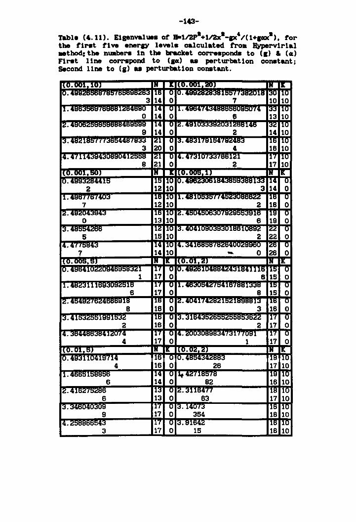
-10-
Table (4.11). Elaenvaluea ot a-112P1+112x1-ax'/(1+laxl ), tor the tlNt tl ve enerlY level. calculated froll !lyperv1rlal _tbod: the nuabera 1n the bracket correapoDda to (I) & (c) Flrat l1ne corrapond to (led ... perturbation constant; Second H08 to (g) ... perturbation constant.
I ( O. ool---!YJ III ~ IlO. 001, IlOJ .11 lA. [0. ,'o~, IUS 0 10 • 11::i::i", ' ____ ,J,8 ;"0 110
3 14 0 7 10 10 11. 1101:ft)O. n 114 0 11.486474 , III 0j0j IIU
0 14 0 6 13 10 12. 4 114 0 2.4811 112B814b ;"2 110
9 14 0 2 14 10 13. 4821~Of f f i 1 cs.,., 121 U OJ.4tS0j11t11b41''':..!4H;j Ib lU
3 20 0 4 16 10 14.47114394 ,1~~~H I~l U ,4. 4'(;"IU'IOj"fDOI~1 1"1 110
8 21 0 2 17 10 I(O.ool,::iOJ III ~ 1(0.005.1J III lit 10. ldiUt; 11::i 110 10. 1.1. 11~~ 114 0
2 12 10 3 14 0 [1.496"'0(403 116 110 11• UIUo.,o, (4. i lb U
7 12 10 2 18 0 12. 4Q7r IA~ 116 110 12 • 4!'i04 , , 116 118 0
0 13 10 8 19 0 13. :A?RR 112 110 1;".4041 118610882 IZZ 0
5 15 10 2 22 0 ~.4775843 114 11U I'" ~41D~:l~, .- I~b U
7 14 10 - 0 28 0 f(0.005,5J III lit 1(0.01,2J l!! ~ 10.48641 "_ 3~1 IH 0 10 .48261 'U841115 115 0
1 17 0 8 15 0 11. 48Z;"nl 1~~15 In 0 11.4 ;,o"15"f~tnOjOj~ 110 U
6 17 0 8 15 0 [2.4!ii ; I 118 116 U I~. 4U411~~~lb~1~tltstslOj Ilb U
8 16 0 3 16 0
13.4' '18815~~ 115 0 13 • 31R4 1!'i3fi~~ IH 0 2 16 0 2 17 0
4. ~(H4,1~U14 i H 0 4. 7;"n IUtll H 0
4 17 0 1 17 0 lO.01,5J ill & ~.~ ]I! ~ 0.49311041871" 115 0 10. _" .- 118 10
4 18 0 26 17 10 1. 46651 114 0 [If 42718578 118 110
6 14 0 82 16 10 2.415Z·fO.::tsD 113 0 IZ. ;"116477 118 110
6 13 0 63 17 10 "3 ~4fin41 3n~ .-~ in U I~. 14013 116 110
9 17 0 354 16 10 4. 117 0 13.91642 lib IIU
3 17 0 15 16 10
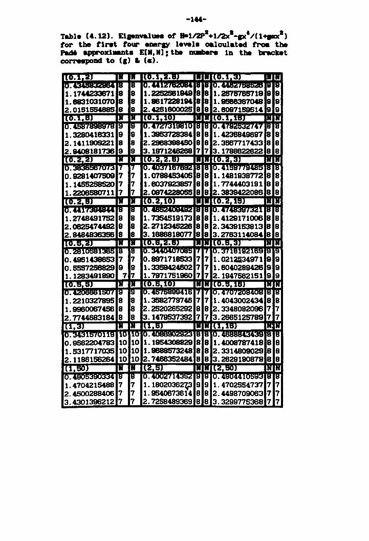
-1"-Table (4.12). El.DValUMI or B-ll2Pa+ll2xa_p'/U..-xa) tor the tiNt tour --I'D' levels calculated troa the Pad6 approxl.anta E[I,N): the m_bera lD the bracket corrnpoDd to (I) la (c).
1(0.1,2) III III IlU.l.2.B) III III IlO.l.3) I. III 10. 18 18 10. KIZ, 18 18 10.USZ, rs re 1.1744233671 8 8 1. 2282981948 8 8 1.2576785719 8 8 1.8831031070 8 8 1.8817228194 88 1.9588387048 8 8 2. o 1515S1885 8 8 2.4251800025 8 8 2.8087158514 8 8 IlU._~.DJ III III IlO.l,10) III III 1l0.l.16) III III 10. 458'I~Ia 18 19 10. ~7V319810 18 18 10. 4"w .... !'C .. ~·/47 18 18 1.3280418331 8 8 1. 3953728384 8 8 1. 4238849687 8 8 2.1411809221 8 8 2.2868388450 8 8 2.3567717433 8 8 2.8408181736 9 9 3.1871248288 7 7 3. 1788822622 8 8 1l0. 2, 2) III III 1l0.2.2.6) III III 1(0.2.3) III I. 10 . .,U'.J 17 17 10.4037167892 18 18 10.41S9',nJ485 jIJ f8 0.9281407S09 7 7 1.07884S3405 8 8 1.1481938772 8 8 1. 14S5258520 7 7 1.6037923857 8 8 1.7744403191 8 8 1.2206580711 7 7 2.0974228055 8 8 2. 3839422086 8 8 1(0.2.5) III IN :(0.2.10) IN IN 1(0.2.15) • IIf 10 •0141', '8 18 iO. 18 18 10. ~74839'132T 8 la-1. 2748491752 8 8 1.7354519173 8 8 1. 4129171006 8 8 2. 062S47M92 8 8 2.2712345228 8 8 2.3439153813 8 8 2.8484836356 8 8 3.1886818077 8 8 3.2783114084 8 8 1(0.5,2) ,ft ft (0.6,2.5) •• I. IlO. 6.:U N IN 10. zsl0581365 8 8 0.~~7085 7 17 10.3718192169 9 9 0.4851438653 7 7 0.8971718533 7 7 1. 0212a34971 9 9 O. 5557268829 9 9 1.3359424802 7 7 1.8040289426 9 9 1.1283491890 7 7 1.7971751960 7 7 2.1947562151 9 9 1(0.5,5) ft • (0.6.10) 11 IN !(0.5.16) N • :0. ,1507 9 9 O.<ag, ,16 7 17 10.4'fUf no 8 8 1.2210327895 8 8 1.3582778746 7 7 1.4043002434 8 8 1.9960067~ 8 8 2.2520265292 8 8 2.3348082096 7 7 2.7744683184 8 8 3. 1479537392 7 7 3.2885125789 7 7 U,3) 11 11 IU.S) 11 ;11 n.15) 11: •• 0.3431570119 110 110 10. r: .. a ,a ,U. fA "X 8 8 0.9562204783 10 10 1. 1954308829 8 8 1.4008787418 8 8 1. 5317717035 10 10 1.8688573248 8 8 2. 3314809029 8 8 2.1186156264 10 10 2. 7466352484 8 8 3. 2629190879 8 8 IU.~) IN III 1(2,5) III I. 1(2.SO) IN IN 10 • AWl 18 18 10.4002714352 19 19 10. 4Q0441,O~~ 18 re-1,4704215488 7 7 1.1802036~ 9 9 1.4702554737 7 7 2. 4500288406 7 7 1.9540673614 8 8 2.4498709083 7 7 3.4301396212 7 7 2. 7258489369 8 8 3.3299775368 7 7
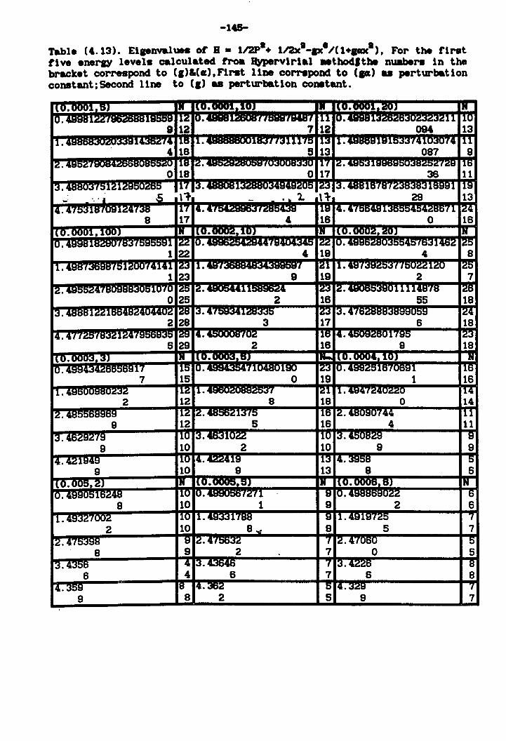
-145-
Table (4.13). ElpnvalUH of B • 112P8+ 112x8 _p l/(1+px8), For the t1rat
t1 Ye enerl)' level. calculated fro. ~rvlrlal _tboclltbe nuabere In the bracket correspond to (,)&(a),Flret 11_ corrapond to (1«) .. perturbatlon constant; Second 11118 to (,) .. perturbatlon constant.
I\O.UUU1,D) III 110.0001.10) III 1(0.0001,20) 111 10. 48881~', 119558 112 IO.&YYH'''''-KL "'~''''''' III IO.4BB8' ~ll 110
9 12 7 12 094 13
11- :'I:oI~1~2°1. 116 11. 0,.,11175 113 11. 1191533'1.103074 rn 4 18 5 13 087 9
12. ,,",O~I 118 12 • 11 117 12.~ :lii'tI 116 0 18 0 17 36 11
13.4: IIo121 ;.1! 117 13.~' 123 13.48818'187 116991 119 ..• : ' iI S \1 ... '1. \l 29 13
14 •4'{OJ187W1247;J8 117 14.47 r( 118 14.4756491 tD'i71 ,24 8 17 4 16 0 16
\0.0001,100) III 110.0002,10) IIf 1(0.0002.20] 1J 0.488818ZI:AHts.:JI 1.1. IZZ 10. ~7gllf14 "014. ... IZZ 10. :4~7631462 25
122 4 19 4 8 [I. 4~tsf.JODOI~.L20074141 z;J 11 ... , I1 21 11.49'( :T(tiOZZ120 :25
1 23 9 19 2 7
12. " il07U 25 12."~.4l" ;23 12. 111114879 128 0 25 2 16 55 18
13. 48881ZZ1 :1U;Z74, 1lUll' '7 Z~ 13 •• , I..tI. 23 13.41 124 .......... 2 28 3 17 6 18
14. 4{ l~olo.:J~124', 28 14." IIUC; :16 14. 11795 [23 6 29 2 18 9 18
\O.UUU~3J ,. (0.0003,8) .... (0.0004.IOJ 11
O. 117 15 0 • .aoaJl~10480180 23 O. 4QQ7~16'rutjSl 116 7 15 0 19 1 16
11- 12 1. rr 121 1 •• ~., IR 2 12 8 18 0 14
12. 4: 12 2.-~~13'15 116 2.~ ' ... 1144 111 9 12 5 16 4 11
3. 46282'n:l 10 3.4631022 110 3 • .4~nR7Q lr 9 10 2 10 9 9
14.4Z1848 110 14. 422.4' a 113 4.~ 5 9 10 9 13 8 5
1(0.005,2) IIf 110.0005,5) IIf 1(0.0006,6) [If
10.4SMII!'l16248 110 10. "~{1 8 10. 177 6 8 10 1 9 2 6
11. 483Z IUU~ 110 11. 48331788 8 11.4918725 7 2 10 8.., 9 5 7
12.4'{O.:J:::Its 8 12 •• 'OO.:J.t: 7 12.47060 '0 8 9 2 7 0 5
13. 430t) 4 13 • .4~~ 7 13.4226 --a 6 4 6 7 6 8
14.358 18 14 .362 5 14.328 7 9 8 2 5 9 7
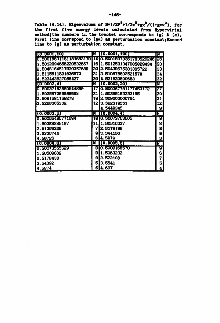
-148-
Table (&.1&). Elgenvalun ot a-ll2Pa+ll2xa+pe/(1+ICXX·>' tor the tlrst tl Ye ener., leve18 calculated tro. Jb'pervlrlal _thod:the nuabera in the bracket corre8pond8 to (I) & (.). First 11ne corraponci to (I.) - perturbation corwtant. Second llne to {Il _ perturbation coD8tant.
1.50508602 2.5178438 3.54392 4.5874
9 1.5063232 9 2.522108 5 3.5541 6 4.607
6 7 5 4
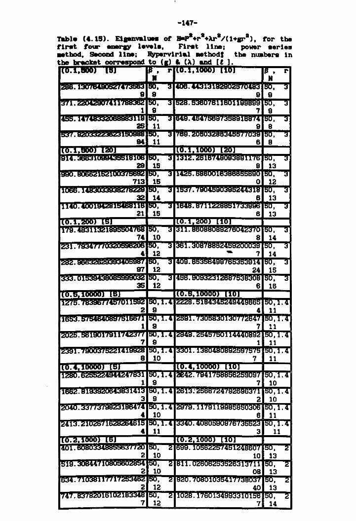
-141-
Table (&.US). Elaenvalun ot a-pl+rl+ArI/U+VI ), tor the tlr.t tour ~ level., Flrat HDaI power •• ri ••
11M; Jb'pervlrlal _tbodl the nuabers In to t .
r
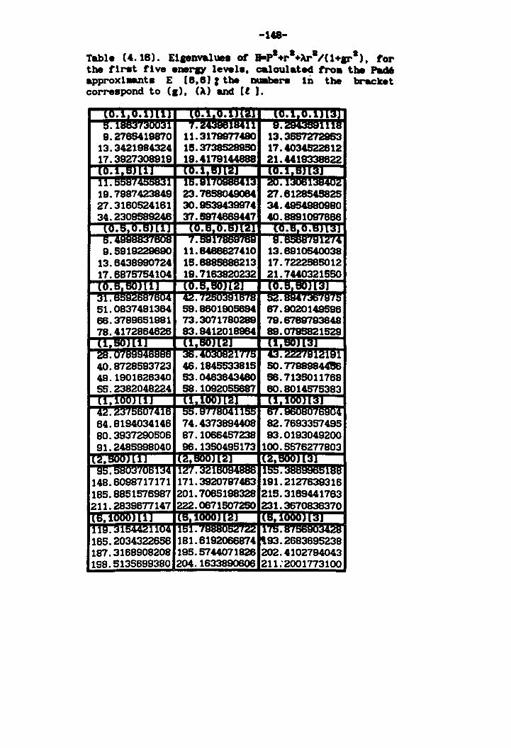
-1.-Table (4.18). Elpnvalues or S-pl+rl+ArI/U+arl ). tor the fh-at fl ve tlDltrm' levela. calculated tro. the PadIt approxl-.nt. E [B. B): the nuabera In the bracket correspond to (,). (A) and [l J •
. 165.2034322656 181.6192066874 93.2683695238 187.3168908208 195.5744071826 202.4102794043 198.5135699380 204.1633890606 211:2001773100
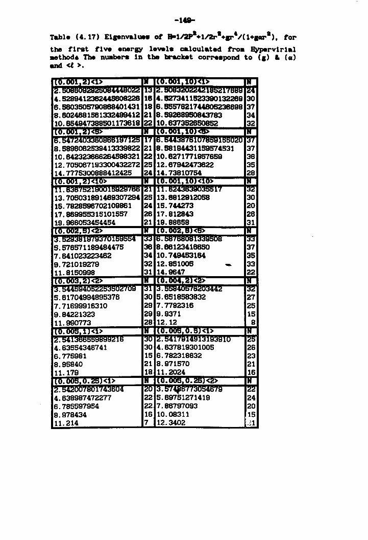
-1G-
Table (4.17) Elsenva1u.. ot H-II2P1+II2rI +cr'/(t+.crl ), tor
the first tl Ye energy level. calculated fro. ~rvlrl .. 1 .. thod. The nUJIbera In the bracket corre.pond to (.) & (Cl) and <t >.
4.638987472277 6.785597954 8.978434 11.214
22 5.69751271419 22 7.86797093 16 10.08311 7 12.3402
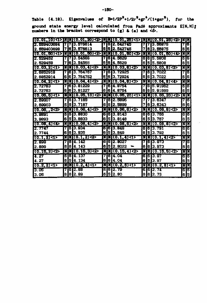
-180-
Table (4.18). Elaenval.. ot B-112P1 +1I2rl +II"'/C1+I«rI). tor the
around .tate enerlY level calculated trom Pad6 approxlant. E[H. MJ, nuaber. in the bracket oorre.poDd to (,) & (.) and <b.
3.05 6 6 2.89 6 5 2.80 662.75 6 5
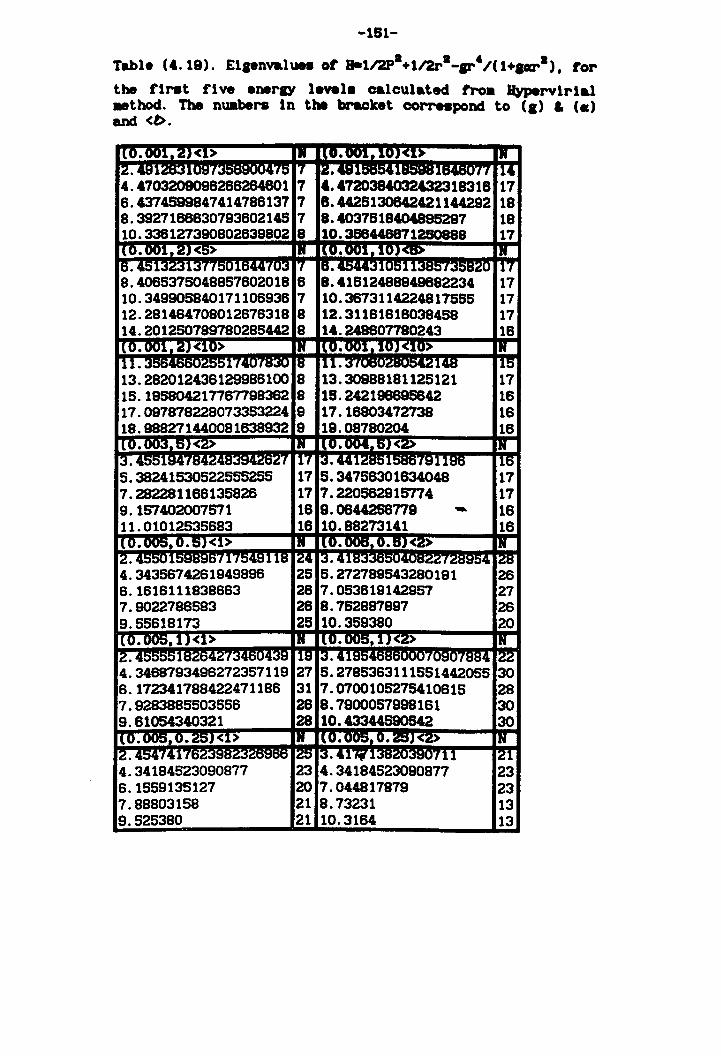
-181-
Table ('.18). E1aenvaluea ot B-lI2P8 +112r8 -art /(1+lcr8). tor
the t1M1t t1 ye enerl)' leYel. calcul .. ted. tro. Jb'perv1rlal .UlOd. The nuabers In the bracket corre.pond to (I) & (.) and <t>.
4.34184523090877 6.1559135127 7.88803158 9.525380
23 4.34184523090877 20 7.044817879 21 8.73231 21 10.3164
23 23 13 13
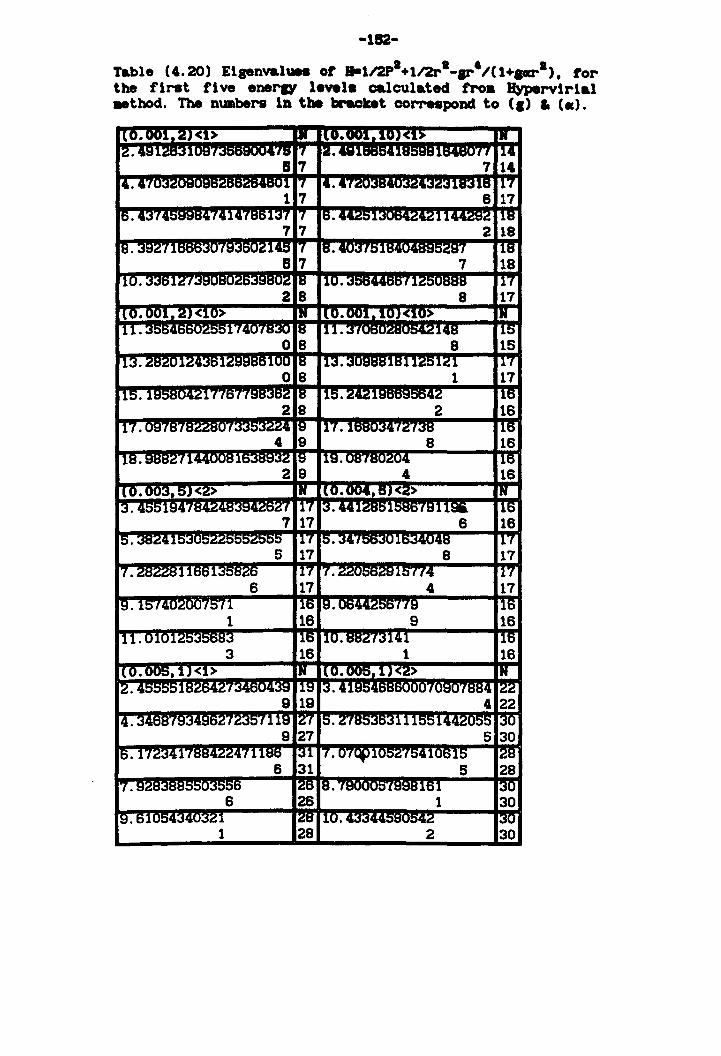
-182-
Table (4.20) E1genval .. ot B-112P1+112r1-.... ' /U+aca-I ). tor the f1rst f1 Ye enerD' leftl. calcula.ted fro. !b'Perv1rlal _tt~d. The nuabera in tbe bNcket oorrnpoDd to (.) • (.).
1 28 2 30
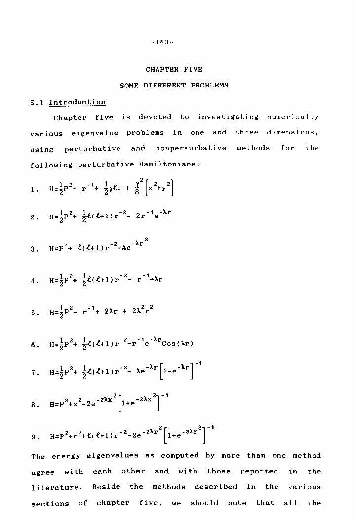
-153-
CHAPTER FIVE
SOME DIFFERENT PROBLEMS
5.1 Introduction
Chapter five is devoted to investigating numericall y
various eigenvalue problems in one and three dimensions,
using perturbative and nonperturbative methods for the
following perturbative Hamiltonians:
1.
2. 1 2 1 2 - 1 -Xr
H = -2 P + -i ( i+ 1 ) r - - Z r e 2 .
3. 2
2 -2 -Xr H=P + t(t+1)r -Ae
4.
5.
6. 1 2 1 - 2 -1 -Ar
H=iP + 2i(-t+l)r -r e Cos(Ar)
7 • 1 2 1 - 2 - Ar [ • Ar] - 1
H=iP + 2 i (t+1)r - Ae l-e
8. 2 2 -2AX -2AX 2[ 2].1
H=P +X -2e l+e
9. 2 2 - 2 .2Xr .2Ar 2 [ 2]-1
H=P +r +-t(t+l)r -2e l+e
The energy eigenvalues as computed by more than one method
agree with each other and with those reported in the
literature. Beside the methods described in the various
sections of chapter five, we should note that all the
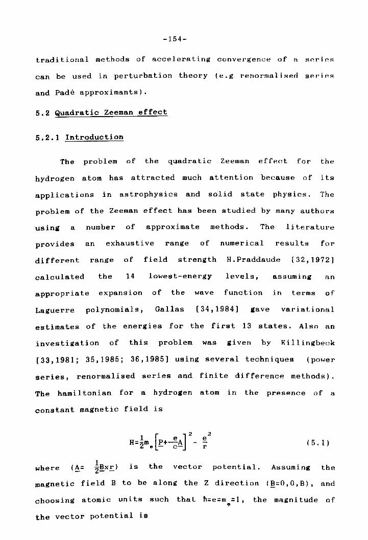
-154-
traditional methods of accelerating convergence of a series
can be used in perturbation theory (e.g renormalised series
and Pade approximants).
5.2 Quadratic Zeeman effect
5.2.1 Introduction
The problem of the quadratic Zeeman effect for the
hydrogen atom has attracted much attention because of its
applications in astrophysics and solid state physics. The
problem of the Zeeman effect has been studied by many authors
usina a number of approximate methods. The literature
provides an exhaustive range of numerical results for
different range of field strength H.Praddaude [32,1972]
calculated the 14 lowest-energy levels, assuminar an
appropriate expansion of the wave function in terms of
Laguerre polynomials, Gallas [34,1984] arave variational
estimates of the energies for the first 13 states. Also an
investigation of this problem was given by Killingbeck
[33,1981; 35,1985; 36,1985] using several techniques (power
series, renormalised series and fini te di fference methods).
The hamiltonian for a hydrogen atom in the presence of a
constant magnetic field is
2 e H= -21
m [P+~A] 2 _ e - c- r ( 5. 1 )
where (~= is the vector potential. Assuming the
magnetic field B to be along the Z direction (~=O,O,B), and
choosing atomic uni ts such
the vector potential is
that h=e=m=l, "
the magni tude of
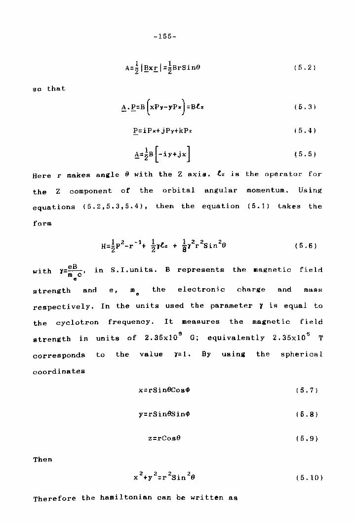
-155-
( 5 .2)
so that
(5.3)
!:=iPx+jPy+kPz (5.4)
~=~B [-iy+jX] ( 5 . 5 )
Here r makes angle 9 with the Z axis. tz is the operator for
the Z component of the orbital angular momentum. Using
equations (5.2,5.3,5.4), then the equation (5.1) takes the
form
(5.6)
with in S. 1. uni ts. B represents the lIagnetic field
strength and e, m e
the electronic charge and mass
respectively. In the units used the parameter 1 is equal to
the cyclotron frequency. It measures the magnetic field
strength in uni ts of 9
2.35x10 G; equivalently 5 2.35x10 T
corresponds to the value J=l. By using the spherical
coordinates
Then
x=rSin8CostP
y=rSin8SintP
z=rCos9
2 2 2. 2 x +y =r SIn 8
Therefore the hamiltonian can be written as
(5.7)
( 5.8)
( 5 • 9 )
(5.10 )
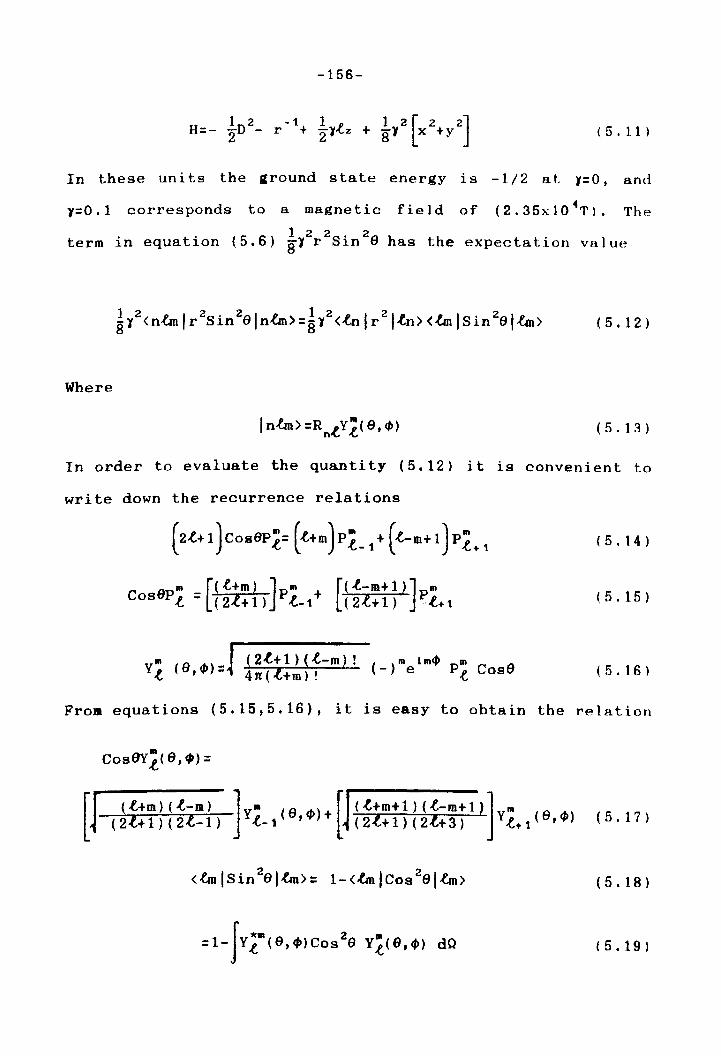
-156-
( 5 . 11 )
In these units the ground state energy is -1/2 at ),=0, and
l'=O.l corresponds to a magnetic field of (2. 35x 1 0 4T ). The
. (5 6) 1 2 2S' 20 h h . term in equation . i} r In u as t e expectatlon value
1 2 I 2 . 2 I ,1_ 1 2 11 I 21'1 I' 2 I g} <n.fin r Sin 8 n~>=gl' <~n r ~n><.fin SIn 8 .fin) (5.12)
Where
( 5. 13 )
In order to evaluate the quantity (5.12) it is convenient to
write down the recurrence relations
m [( t+m) ] m Cos8P t = (21+ 1) p .(.-1 + [
( t-m+ 1 )] m (2:t+1) p .(.+1
(5.14 )
( 5 . 15 )
( 5 . 16 )
From equations (5.15,5.16), it is easy to obtain the relation
( 5. 17 )
(5.18)
( 5. 19 )
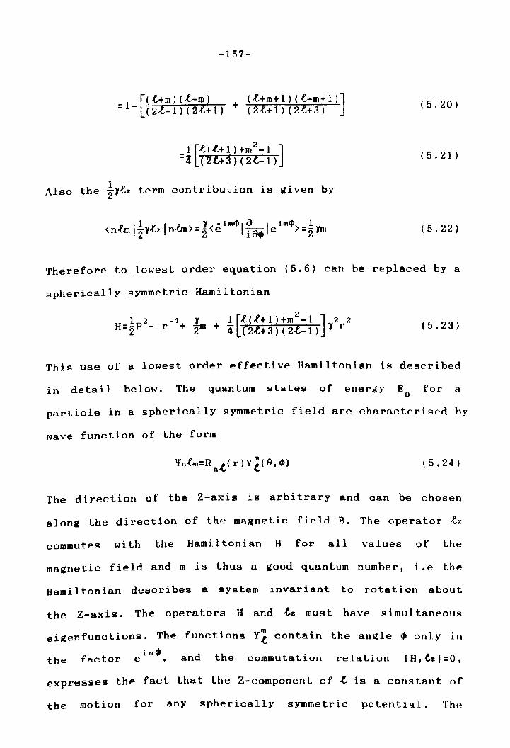
-157-
_ [(t+m)(t-m) (t+m+l)(t-Il+1)] -1- (2l-1)(2l+1) + (2l+1)(2l+3)
(5,20)
(5,21 )
h I 11 t 'b t' . , b Also t e 21~z term con r1 u 10n 1S g1ven y
(5.22)
Therefore to lowest order equation (5.6) can be replaced by a
spherically symmetric Hamiltonian
1 2 -1 J 1 ,f,(,f,+l)+m -1 2 2 [ 2] H=2P - r + rn + 4" (2l+3)( 2l-1) J r (5.23)
This use of a lowest order effective Hamiltonian is described
in detail below. The quantum states of energy E o for a
particle in a spherically symmetric field are characterised by
wave function of the form
(5.24 )
The direction of the Z-axis is arbi trary and can be chosen
along the direction of the magnetic field B. The operator tz
commutes with the Hamiltonian H for all values of the
magnetic field and m is thus a good quantum number, l.e the
Hamil tonian describes a system invariant to rotation about
the Z-axis. The operators Hand ,f,z must have simul taneous
eigenfunctions. The functions Yt contain the angle ~ only in
the factor imtl>
e and the commutation relation [H, tz 1 =0,
expresses the fact that the Z-component of L is a constant of
the motion for any spherically symmetric potential. The
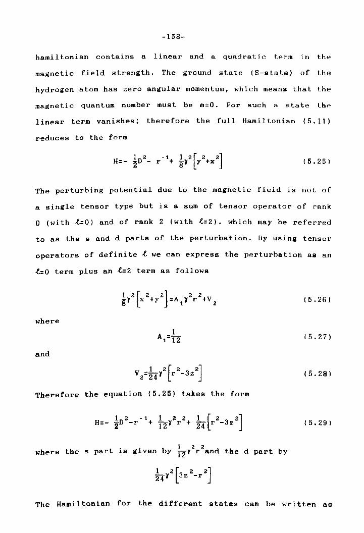
-158-
hamiltonian contains a linear and a quadratic term in the
magnetic field strength. The ground state (S-state) of the
hydrogen atom has zero angular momentum, which means that the
magnetic quantum number must be m=O. For such a !'ltate thf~
linear term vanishes; therefore the full Hami 1 tonian (5.11)
reduces to the form
(5.25)
The perturbing potential due to the magnetic field is not of
a single tensor type but is a sum of tensor operator of rank
o (with ~=O) and of rank 2 (with {=2). which may be referred
to as the sand d parts of the perturbation. By using tensor
operators of definite ~ we can express the perturbation as an
~=O term plus an t=2 term as follows
where
and
1 A 1=12
Therefore the equation (5.25) takes the form
t " " b 1 22 d where the spar 1S g1ven y 121 r an the d part by
1 2[ 22] '241 3z-r
(5.26)
( 5.27)
( 5 • 28 )
(5.29)
The Hamiltonian for the different states can be written as
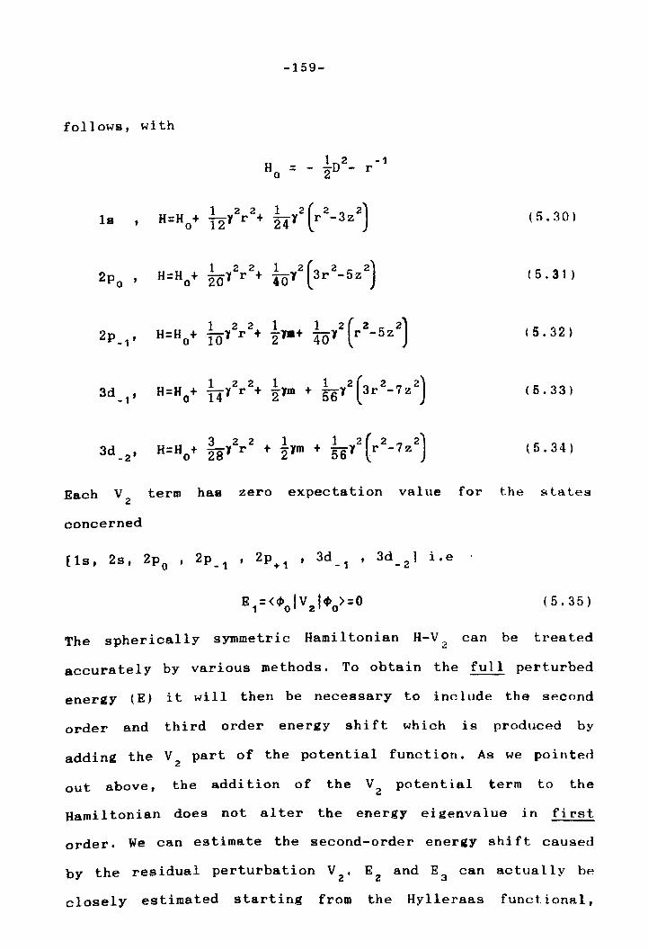
-159-
follows, with
Ho 1 2 -1
= - "2D - r
Is H=H + 0
122 ill' r + 1 2( 2 2) '241 r -3z ( 5.30)
2po ' H=H + 0
122 20l' r + 1 2( 2 2) 40" 3r -5z (5.31)
122 1 1 Z (2 2) 2p -1' H=H + IOlr + -}a+ 40" r -5z 0 2
(5.32 )
H=H + 122 1 1 2( 2 2)
3d -1' IT1 r + -lm + 56 1 3r -7z 0 2 (6.33 )
H=H + 3 2 Z 1 1 2( 2 2)
3d -2' 28 1 r + -lm + 56 1 r -7z 0 2
( 5 • 34 )
Each V2
term has zero expectation value for the statps
concerned
The spherically symmetric Hami 1 tonian H-V 2
can be treated
accurately by various methods. To obtain the full perturbed
energy (E) it will then be necessary to include the second
order and third order energy shift which is produced by
adding the V2
part of the potential function. As we pointed
out above, the addi tion of the V 2 potent ia1 term to the
Hamil tonian does not al ter the energy eigenvalue in f1 rst
order. We can estimate the second-order energy shift caused
by the residual perturbation V2
, E z and E3 can actually be
closely estimated starting from the Hylleraas functional,
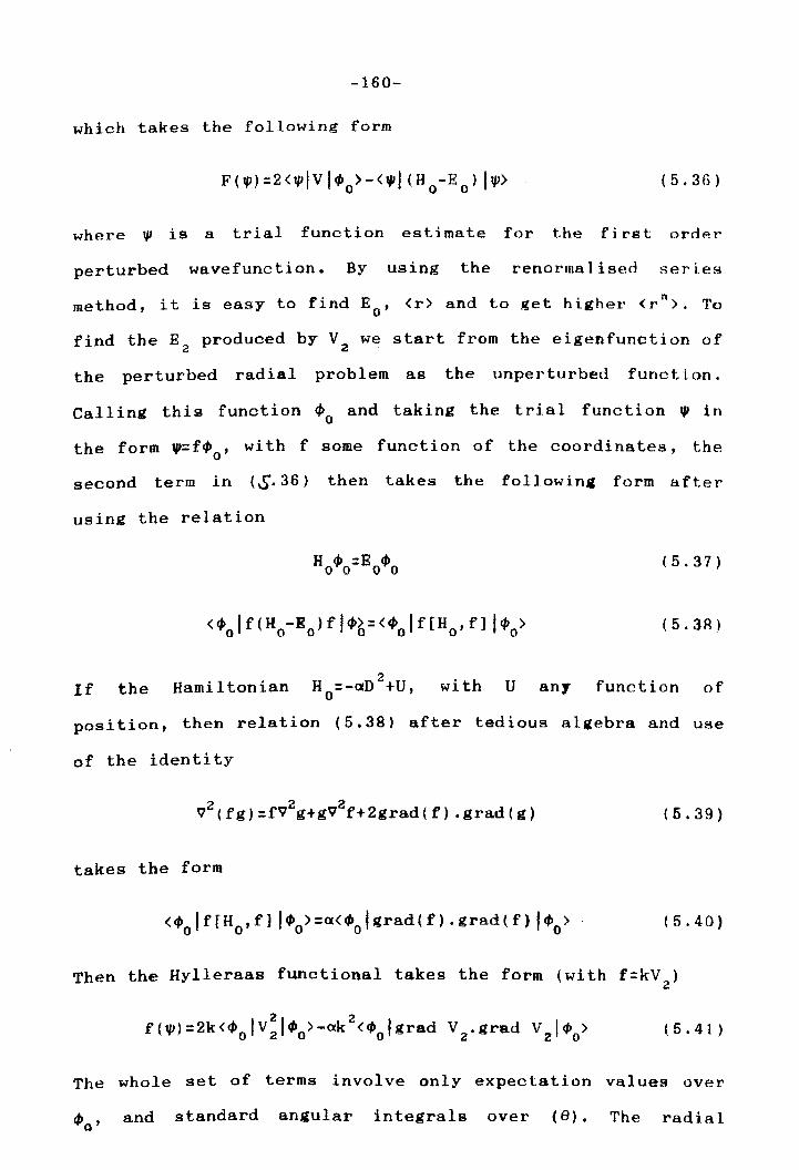
-160-
which takes the following form
(5.36)
where tp is a trial function estimate for the fi rat order
perturbed wavefunction. By using the renormalised series
method, it is easy to find Eo' <r> and to get higher (ro>. To
find the E2 produced by V2
we start from the eigenfunction of
the perturbed radial problem as the unperturbed function.
Calling this function 4>0 and taking the trial function '" in
the form ",=f4>o' with f some function of the coordinates, the
second term in <S. 36) then takes the followin~ form after
using the relation
If the Hamiltonian
H ..t. -E ..t. 0"'0- 0"'0
2 Ho=-aD +U,
(5.37 )
(5.3B)
with U any function of
position, then relation (5.38) after tedious algebra and use
of the identity
2 2 2 V (fg)=fV g+gV f+2grad(f) .grad(g) (6.39)
takes the form
(5.40)
Then the Hylleraas functional takes the form (with f=kV2
)
(5.41)
The whole set of terms involve only expectation values over
.0' and standard angular integrals over (8). The radial
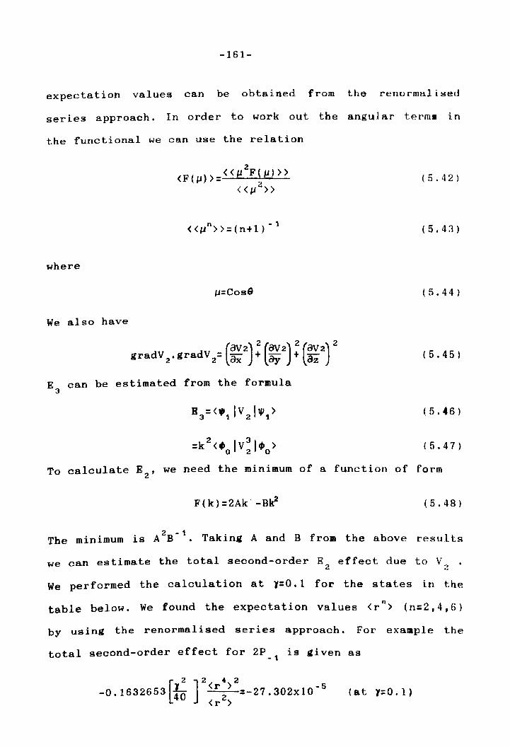
-161-
expectation values can be obtained from the renormaliserl
series approach. In order to work out the angul ar terms in
the functional we can use the relation
(5.42 )
«lJn»=(n+l) -1 (5.4~)
where
lJ=Cos8 (5.44)
We also have
(5.45)
E3 can be estimated from the formula
( 5.46)
(5.47)
To calculate E2
, we need the minimum of a function of form
F(k)=2AkO -B~ (5.48 )
The minimum is A2B-
1• Taking A and B from the above results
we can estimate the total second-order E2 effect due to V2
We performed the calculation at 1=0.1 for the states in the
table below. We found the expectation values <rn> (n=2,4,6)
by using the renormalised series approach. For example the
total second-order effect for 2P is given as - 1
( at 1=0. 1 )
-162-
and also the total third-order effect for the same slate 2P - 1
is given as
[L2 J3[ 2 32 6 ] -5 40 2k (-3T)<r > =-4.78852x10 (at 1=0.1)
where the value of k it can be determined from the
- 1 second-order calculation and equals k=AB . The perturbation
coefficient in the above calculat i on is (.,2/ 40 ), wh ich i ~
actually (A) (see (5.32». The (H-V2
) energy eigenvalue for
state 2p is -0.1505220 as found by the renormalisd series - 1
approach, which also gives expectation values 2 <r >=21.1594,
.. 6 <r >=752.424,<r >=38967.179. The second and third order
shifts due to are estimated to be (-0.000302,
-0.0000478852) respectively. The second-order correct ion to
the energy is six times the third-order correction, Ez and E3
together give a corrected energy (-0.1508429). This energy is
in good agreement with Praddaude; using a large scale matrix
calculation he obtained (-0.150845). The second and thi I'd
order corrections thus bring our results closer to the
resul ts of Praddaude and indicate that it is sufficient to
take the second and third order corrections to obtain a 1000
energy. The unperturbed 2p_1energy is -1/8, so the V1
part of
the perturbation has given an energy shift (-0.025522), while
V has given a second order shift (-0.00027302) and a third 2
order shift (-0.0000478852). The calculation described above
can be carried out for various other states, as shown in
table (5.2), which gives the required express ions for each
state.
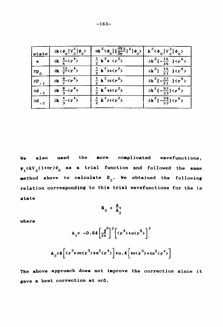
-163-
state 2k<4»oIV~I4>o> cxk 2 <4» I [avZ]214» > o or 0 k2<4» IV
314» > 020
2k ~<r4) 1 k 2s <r2) k2[ 16 1<r6) s - 2 --
5 2 35
2k g<r4> 1 2 2 2k2 [ 16 J<r6) apo - k 24(r ) -7 2 21
ak !!-<r4) 1 k 216<r2) k2 [ 32 1<r6
) 2P 2 2 --- 1 7 21
2k !!-<r4) 1 2 2 2k 2[_E]<r 6 ) 3d - k 4s<r ) - 1 3 2 33
2k ~<r4) 1 2 2 2 38 6
3d - k 24<r ) 2k [--l<r ) -2 3 2 33
We also used the more complicated wavefunctions,
a trial function and followed the same
method above to calculate B2 • We obtained the followina
relation corresponding to this trial wavefunctions for the 1s
state
where
The above approach does not improve the correction since it
gave a best correction at «=0.
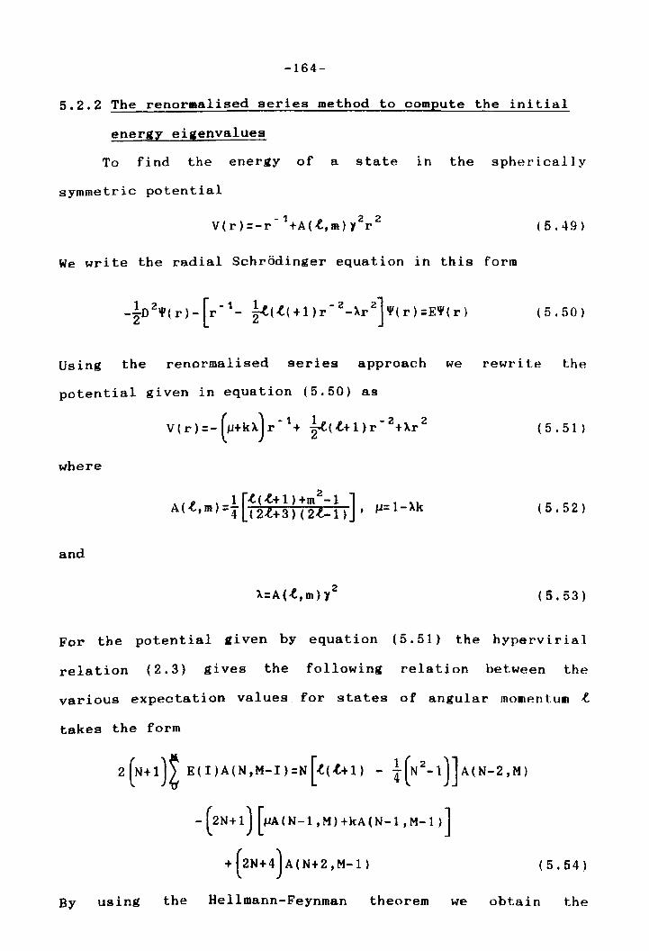
-164-
5.2.2 The renormalised series method to compute the initial
energy eigenvalues
To find the energy of a state in the spherically
symmetric potential
-1 11 2 2 V(r)=-r +A(-\"m)l r ( 5 • 49 )
We write the radial Schrodinger equation in this form
(5.50)
Using the renormalised series approach we rewrite the
potential given in equation (5.50) as
where
and
( ) -1 1 11 -2 2
V(r)=- p+kX r + ~(-\'+1)r +Ar
2 A=A(,(.,m)l
(5.51)
( 5.52 )
(5.53)
For the potential aiven by equation (5.51) the hypervirial
relation (2.3) gives the following relation between the
various expectation values for states of angular mOllentull t
takes the form
2 (N + 1 ) i E ( I ) A ( N , M - I ) = N [ t ( .t+ 1) - t ( N 2 - 1) ] A ( N - 2 , M )
- (2N+1) [1JA(N-l,M)+kA(N-l ,M-1 >]
+ (2N+4)A(N+2 ,M-l) (5.54)
By using the Hellmann-Feynman theorem we obtain the
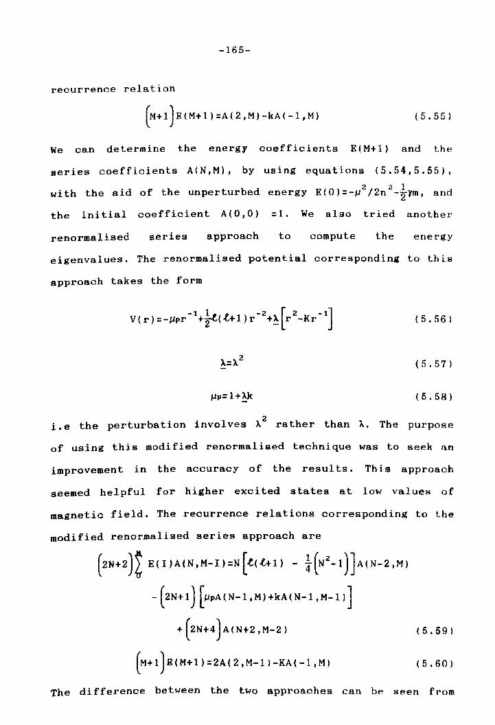
-165-
recurrence relation
(M+l)E(M+1):A(2,M)-kA(-1,M) ( 5 • 55 )
We can determine the energy coefficients E(M+l) and the
series coefficients A(N,M), by using equations (5.54,5.55),
221 with the aid of the unperturbed energy E(O)=-p /2n -2¥m, and
the ini tial coefficient A (0,0) : 1. We also tried another
renormalised series approach to compute the energy
eigenvalues. The renormalised potential corresponding to this
approach takes the form
-1 1. 1# - 2 [2 -1] V(r)=-ppr +~(~+l)r +~ r -Kr ( 5 • 56 )
(5.57 )
(6.58)
2 i.e the perturbation involves X rather than X. The purpose
of using this modified renormalised technique was to seek an
improvement in the accuracy of the resul ts. Th is approach
seemed helpful for higher excited states at low values of
magnetic field. The recurrence relations corresponding to the
modified renormalised series approach are
( 2 N + 2 ) t E ( I ) A ( N , M - I ) = N [ t ( .f.+ 1) - t ( N 2
- 1 ) ] A ( N - 2 , M )
- (2N + 1) [IJPA ( N - 1 , M) + kA ( N - 1 , M - 1 ) ]
+ (2N+4)A(N+2,M-2)
~+1)E(M+l):2A(2,M-l)-KA(-1'M)
( 5 . 69 )
(5.60)
The difference between the two approaches can be seen from
-166-
equations (5.54,5.55.5.59,5.60), in the third term and first
term of the right hand sides of the equations. The same
technique was used for anharmonic oscillators in chapter 2
and helped to compute energy eigenvalues for 6 8
(~x ,~x )
perturbations which were an improvement over those given by
the usual approach.
5.2.3 Results and discussion
We have calculated energy levels for all thirty states
which have principal quantum number n=1,2,3,4, for magnetic
field strengths in the range 0.005s 1s0.01. Also we calculated
thirteen states with (n=1,2,3) at 1 =0.1. We computed the
results using the renormalised series approach. Our results
are converged to (14-figures) at field values corresponding
to 1=0.005 and 1 =0.01. This accuracy decreases for higher
states. While the ordinary renormalised series (~I,I=l) does
I not work at 1=0.01 and n=4, the other approach (X, 1=2) works
satisfactorily. Our results at 1=0.005 are in good agreement
with the results of Gallas[34,1984], which are converled only
to four significant filures. Two considerations govern our
calculation at low magnetic fields; first, to show that the
two perturbation approaches work very well and, second, to
compute the energy eigenvalues for higher states. In table
(5.3), it is clear that the renormalised series method for
H-V gives a very good upper bound to the total energies, 2
while using the second and third order correct ions to the
energy bring our results very close to the results obtained
by Praddaude; this is clear from table (5.2). Killingheck
[14,1981] estimated second-order corrections, so our work is
-167-
an extension of this work. Table 5.1 shows the expectation
value for (r n), table 5.2 shows the energy and the second and
third order corrections to the energy. Table (5.4) shows that
the agreement between the results of the two perturba t ion
approaches are very satisfactory at (1=0.1) for states with
n=1,2. The number of coefficients required to get a converged
energy eigenvalue from the renormalised series is less with
the X2 approach; this is clear from our results as shown in
the tables (5.4,5.5). We believe our results demonstrate that
the renormalised series method work excellently for low
range values of magnetic field (where the series converge
quickly) but does not work for high values of magnetic field.
The energy eigenvalue associated with the 2p(+1) state can
easily be calculate from the results for the 2P(-1) state.
The term the linear Zeeman term 1n equat.ion
(5.30-5.31); for the 2p(-1) state we have m=-1 and for the
2p{+1) state we have m=1, therefore they differ in energy by
amount (I),which means that to get the energy eigenvalue for
the 2p(+1) state it will only be necessary to add this amount
to the resulting energy for the 2p(-1) state. In a similar
way we can compute the ener,y eigenvalues for the other
states; therefore states with m)O canno~ treated separately,
since B(t,m)-E(t,-m) has the fixed value ml.
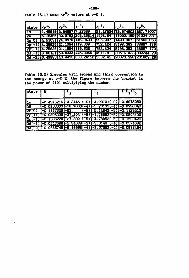
-168-
Table (5.1) some <rD) values at 7-0.1.
Table (5.2) Energies with second and third correction to the energy at 7=0.1: the figure between the bracket ls the power of (10) multiplying the number.
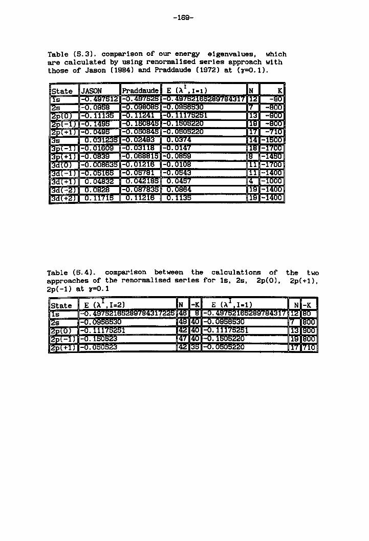
-169-
Table (5.3). comparison of our energy eigenvalues, which are calculated by using renormalised series approach with those of Jason (1984) and Praddaude (1912) at (~=O.l).
Table (5.4). comparison between the calculations of approaches of the renormalised series for ls, 2s, 2p(O), 2p(-1) at ~=O.l
the two 2p(+1),
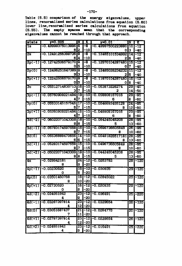
-170-
Table (5.5) comparison of the enerlY eigenvalues. upper lines. renormalised series calculations from equation (6.80) lower line. renormalised series calculations from equation (5.65). The eapt)' apaces _an that the correspondina eigenvalues cannot be reached through that approach.
9 -20

-171-
Table (5.5 contlnued)
4f(-3) -0.031185612 26 -280 2
2 13 -20
-172-
5.3 Hydrogen atom with a Yukawa potential
The general screened Coulomb potential for hydrogen like
atoms may be written in the form
-1~ n V(r)=-Zr L Vn(Xr)
n.O (5.61)
where Z is the nuclear charge and X represents the screening
constant. Screened Coulomb potentials have received a great
deal of attention , not only in the field of nuclear physics
but also in other fields such as atomic, solid state and
plasma physics. The problem of the Yukawa potential has been
studied by many authors, employing different approaches.
C.S.Lai [38,1984] obtained, using Pade approximants [6,6] and
[6,7], the energy eigenvalues for different values of X and
for various eigenstates. Rdward R. Vrscay [39,1985] developed
a power series method to calculate to large order the
Rayleigh-SchrOdinger perturbation expansions for energy
levels of a hydrogen atom with a Yukawa type screened Coulomb
potential, treating the 1s, 2s and 2p levels. We employ the
Hellmann-Feynman theorem and the hypervirial theorem to
calculate the energy eigenvalues of various energy
eigenvalues to high accuracy. In our work we wish to show
that the renormalised series method can be used to calculate
the bound-state energies of a screened Coulomb potential to
very high accuracy. The present section treats the Yukawa
potential. This study was motivated by the work of Lai
[38,1984], who observed that [N-1,N] and [N,N]
approximants to the energy series provide accurate estimates
of eigenvalues. The method which he used raises the question
-173-
of whether or not the renormal ised series method can gi ves
accurate estimates of the eigenvalues. The two approaches
(his and ours) which have been employed to study the
potential use the Hellmann-Feynman and hypervirial theorems
but our approach uses no Pade approximants. The renormalised
series method for this problem is complicated by the presence
of the renormalisin, constant K. A proper treatment would
necessarily involve the choice of an ideal value for the
renormalising constant K. The Hamiltonian for the Yukawa
potential can be written as
1 2 1" -2 Z -1 -~r H= - 2D + ~(~+1)r - r e (5.62)
• _ ~2+ tt(.f.+l)r- 2 -Z(J./+MC)r- 1 -zr- 1! Vn(~r)n na 1
where
J./=1-UC
where t is the orbital an,ular momentum quantum number. Here
we are usin, atomic units, h=e=m=1. By employing the
Hellmann-Feynman theorem and the hypervirial theorem as in
previous sections the followin, two relations are obtained
- (2N+l) [J.IB(N-l ,M)+KB(N-l ,M-I)]
-2 vn (2N+n+2)B(N+n,M-n-l) naO
(5.63)
-174-
(5.64 )
The coefficients V in (5.63) and (5.61) can be written as n
V =(_1)n+l
n (n+1)! (5.65)
for the case of the Yukawa potential. The coefficients V 1n n
aeneral alternate in sian and decrease with increasing n. 2 '"
Where the eneray of the unperturbed nth state E(O)=-~ /2n'· is
known, the equations (5.63,5.64) suffice to calculate the
full set of E and B coefficients, with the aid of equation
(5.65) and the startina term B(O,O) which is obtained from
the condition of normalization o
<r >=<1>=1. Our numerical
results, presented in table (5.6), reveal that at low values
of ~ for states (ls,2s,2p) we have excellent aareement with
the values of Edward R.Vrscay [39,1985]. Our approach
provides extremely accurate eiJenvalues at low A. These
values are accurate to all the diJits shown and agree to over
(19) diJits with those of Vrscay. The power of this
renormalised series techniques at low values of A has thus
been demonstrated. However, at larJer values of A, the
accuracy decreases as expected from our previous renormalised
series calculations, al thouah the accuracy is better than
that of Lai [38,1984].
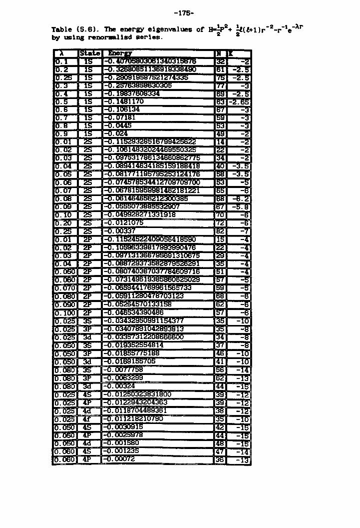
-175-
Table (5.6). The energy eiaenvalues of s-iP2 + itCt+1 )r -2_r -le -).r by using renor.allsd series.
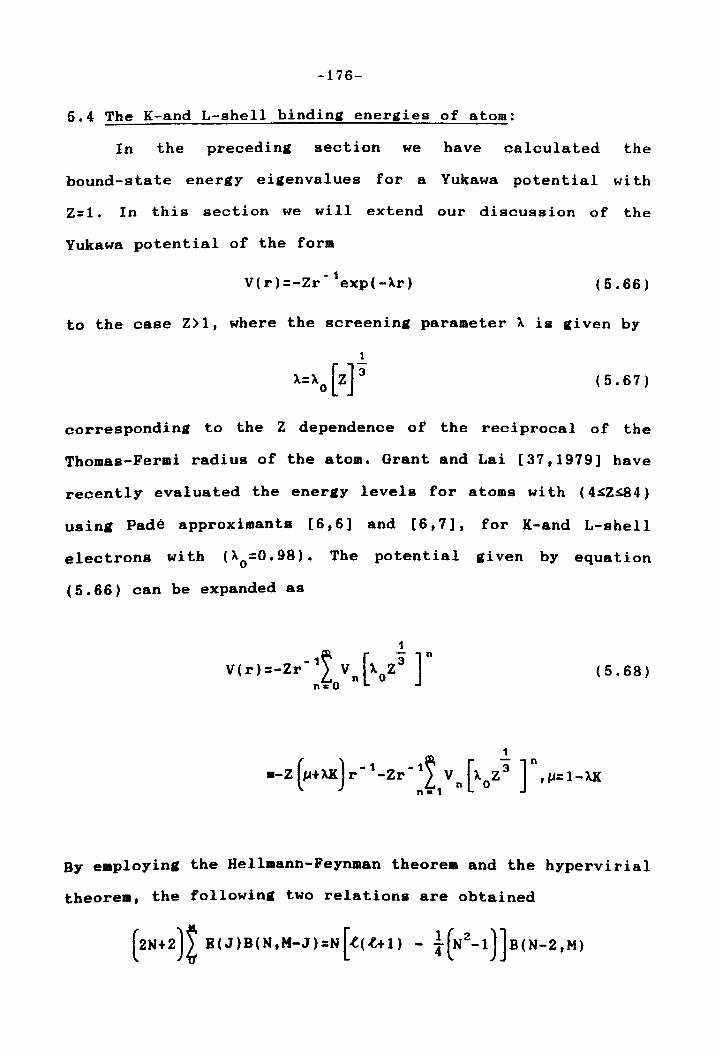
-176-
5.4 The K-and L-shell bindine enereies of atom:
In the precedine section we have calculated the
bound-state energy eieenvalues for a Yukawa potential wi th
Z=l. In this section we will extend our discussion of the
Yukawa potential of the form
- t V(r)=-Zr exp(-lr) (5.66)
to the case Z>l, where the screening parameter 1 is given by
(5.67)
correspondine to the Z dependence of the reciprocal of the
Thomas-Fermi radius of the atom. Grant and Lai [37,1979] have
recently evaluated the energy levels for atoms with (4~Z~84)
using Pade approximants [6,6] and [6,7], for K-and L-shell
electrons with (10=0.98). The potential given by equation
(6.66) can be expanded as
(5.68)
By eaploying the Hellmann-Feynman theorem and the hypervirial
theorem, the following two relations are obtained
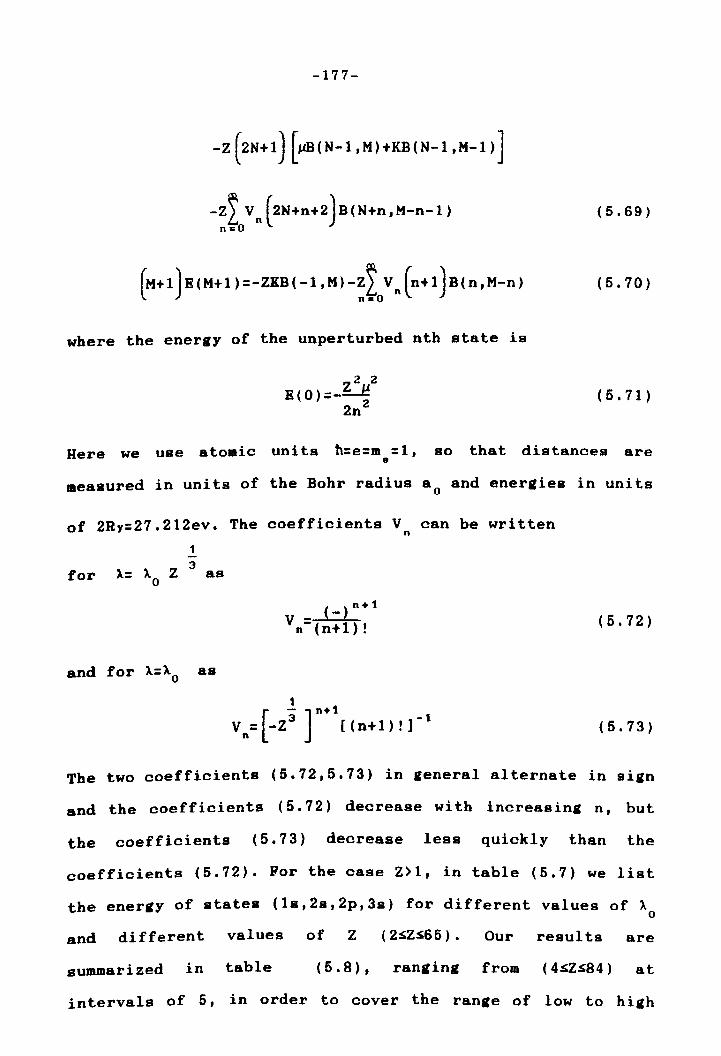
-177-
-z (2N+l) [~(N-l ,M)+KB(N-l ,M-l)]
where the energy of the unperturbed nth state is
2 2
R(O)=-~ 2n2
(5.69)
(5.70)
( 5 . 71)
Here we use atomic units h:e:m :1, e
so that distances are
measured in units of the Bohr radius a o and energies in units
of 2Ry:27.212ev. The coefficients V can be written n
for
and for ~=~ as o
3 -1 [ .!]n+1 V n: -Z [ (n+ 1) ! ]
(5.72)
(5.73)
The two coefficients (5.72,5.73) in general alternate in sign
and the coefficients (5.72) decrease with increasing n, but
the coefficients (5.73) decrease less quickly than the
coefficients (5.72). For the case Z)l, in table (5.7) we list
the energy of states (1s,2s,2p,3s) for different values of ~ o
and different values of Z (2~Z~65). Our results are
summarized in table (5.8), ranging from (4~Z~84) at
intervals of 5, in order to cover the range of low to high
-178-
atomic number. For a given shell the resul ta improve with
increasing Z, but the accuracy of the results decreases as
we go to higher shells. The renormalised series approach as
introduced by Killingbeck is a very elegant and powerful
approach to compute the energies eigenvalues with high
accuracy. The approach achieved an accuracy of fifteen
significant figures for higher values of atomic number Z; to
our knowledge such a high degree of accuracy for the
eigenvalues of the Yukawa potential has never been obtained
by any other method. As a next comment we wish to draw
attention to the fact that the renormalised series work
1/3 equally well for ~=~o and A=~OZ as perturbation parameter;
we used the two values of ~ in order to verify the accuracy
of the renormaliaed series for this calculation. Using two
different value of screening parameter provides alternative
approaches for computing energy eigenvalues. The calculated
energy eigenvalues diverge at low atomic number Z, for the
K-shell, whereas the series will work for zero values of the
renormalising constant for Z>29.
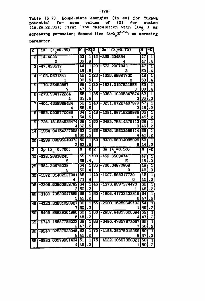
-179-
Table (5.7). Bound-state energies (in ev) for Yulcawa potential for some values of (Z) for states (ls, 2s, 2p, 35); First line calculation wl th (~-~ ) as
8creening parameter; Second line (A-~OZl/2) as acreelng
parameter.
4 45 .2 1 50 .2
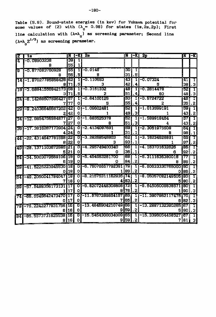
-180-
Table (5.8). Bound-state energies (in kev) for Yukawa potential for some values of (Z) with (Ao= 0.98) for states (ls,2s,2p); First
line calculation with (A=Ao) as screening parameter; Second line
(A=A Zl/3) as screening parameter. o
IZ ls IN -It 2s N -K 2p [4 -0. IH!-Il ~1/'~11 139 1
8 55 1 '9 -0. 01 loo.;iIOu~c:;a ltiti 1 -0.0148 30 1
8 56 .5 8 31 .5 :14 -1. 'd/Uet-11 le~ 1 -0.110653 43 1 -u. U"~~4
8 71 .5 3 42 .4 5 19 -3.68841556B4zn~ ItiH 1 -0.3151332 4B 1 -0. ZtH44;fB
3 71 .5 2 51 .4 80
124 -e. 1 4:;...oHHhlll ilJ.~" 57 1 -U.e41001~ti 50 1 -u. t:HZ4"1ZZ 7 77 0 5 55 .4 2
[29 -9. 74r "C:;UC:; 4~ 0 -1. sn 5~ 1 -1. 01~o99191 2 42 0 1 49 .3 1
134 -12.tI'dot,l,l 77 ~'( ° -1. 11'd 52 1 -1. 58991H404
7 27 0 8 51 .3 4
[39 -17.3HI6Zt:ff173904 ~4 0 -2. 41;;'4U~H6~1 ti~ 1 -Z.~051975508 4 24 0 1 31 .1 8
44 -~~.4314047781598 2~ U -3. :~ 62 1 -3. I HZ~IJ.' ~I1I1H 1 8 22 0 3 93 .1 1
49 -ZB.13711U~t)IGo;Joo;J 21 ° -4. ~~ti'f 1J.~lJ.nr-~lJ.r 166 1 -4. 10~HUlr'i~1.Oo':h"'-h 5 21 0 0 36 .1 6
54 -~4. tiUl.~1U Itloo~106 118 U -ti.IJ.~, '1-'00 16B 1 -ti.311lfi [118 6 19 0 0 84 .2 8
[59 -41. ~:;.I:;.I~7Z~QIJ.~~·~( 118 0 -e. {t)U 1660 IIl::IZ~l::Il 78 1 -6. II
0 18 0 1 89 .2 0
164 -4~. :;.IlIhLJl ,1784047 lIB 0 -8.2157531116Z~~0 74 1 -8. UOUO/UH~lIJ.QR' IR 7 18 0 4 83 .2 5
169 -57. ~nQQ~"'~l'(~l~l 117 U -~. Het-Ut LIJ. 172 1 -9. R4 I~"fl
1 17 0 8 76 .2 1
74 -66. :JJ: 473470 '17 0 -11. 010/ i4,157 169 1 -11. 390', tfo.G 11 'r 4"16
0 17 0 7 65 .2 6 79 -·(e. 774:;.1.:;.I,lll::IJI756 le U -13. 4R4H!-I( IIJ.:;.I ,0749 66 1 -1~. ~BB'fl:~7:u~n7R!'i
6 16 0 9 59 .2 5
84 -Hti. tiOI~I.:sli 10 ° -15.!'i4!'i4~nnn~4nn~ 65 1 -15. i41J. IOc:;{
8 16 0 9 59 .2 7
N -It
41 1 38 .3
15Z 1 48 .3
149 1 35 .2 159 1 43 .2 lti·, 1 43 .2 164 1 98 .1
169 1 97 .2 ~B6 1 92 .2 77 1 89 .2 ~U 1 86 .2 ,BO 1 80 .2 IBU 1 90 .3 1U 1 82 .3 167 1 80 .3 16'1 1 81 3
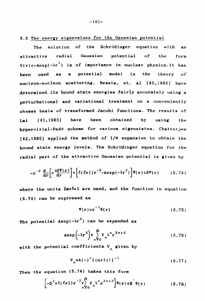
-181-
5.5 The energy eigenvalues for the Gaussian potential
The solution of the Schrodinger equation with an
attractive radial Gaussian potential of the form
'" V(r)=-Aexp(-Xr~) is of importance in nuclear physics.It has
been used as a potential model in the theory of
nucleon-nucleon scattering. Bessis, et. al [40,1982] have
determined its bound state energies fairly accurately using a
perturbational and variational treatment on a conveniently
chosen basis of transformed Jacobi functions. The results of
Lai [41,1983] have been obtained by using the
bypervirial-Pade scheme for various eigenstates. Chatterjee
[42,1985] applied the method of 1/N expansion to obtain the
bound state energy levels. The Schrodinger equation for the
radial part of the attractive Gaussian potential is given by
(5.74)
where the units 2m=b=1 are used, and the function in equation
(5.74) can be expressed as
- 1 V(r)=r 41(r)
2 The potential Aexp(-Xr ) can be expanded as
with the potential coefficients V given by n
V =A(_)n[(n+1)!]-1 n
Then the equation (5.74) takes this form
[ 2 p p - 2 ~ n 2 n + 2] I
-D +~(~+l)r +L VnX r 41(r):B ~(r) n.O
(5.75)
(5.76 )
(5.77)
(5.78)
-182-
with E =E+A. The function ~(r) must vanish at r=O. Now,
applying the hypervirial theorem, the Hellmann-Feynman
theorem and using equation (5.77), the relation between the
coefficients B(N,M) and the energy coefficients E(M) can be
expressed as
+2 Vn [2N+2(n+2)]B(N+2(n+l»,M-n-l) n.O
(5.79)
(5.80)
The unperturbed value of B is given by
B(O)= [(4n+2.t+3 }fAJ-A (5.81)
where n is the principal quantum number, -t the angular
momentum and we set A=400 to agree with previous authors. The
recurrence relations (5.79,5.80) with equation (5.81) and
initial condition A(O,O)=l can be used to evaluate the energy
coefficients E (M) • The success and power of the method may
strongly depend on the state and the angular momentum. The
convergence rate decreases noticeably as (.t&n) increase, as
shown in table (5.9). This situation occurs in all problems
involving eigenvalues in perturbation theory. The
calculations show that the present procedure converges more
quickly and accurately at low values of (-t&n). Our resul ts
are very accurate in this low range. The degree of agreement
between our results and those arising from other methods is
very good, both for ground and exci ted states. For -f..> 7 we
-183-
have not found numerical results in the literature, but our
results show the eigenvalues for these states. Our main goal
is to show that the energy eigenvalues of the attract i ve
radial Gaussian potential calculated from the hypervirial
method are in good agreement with other numerical results. We
notice from table (5.9) that for the ground state and some of
the first few excited states at low value of angular momentum
we find the energy values with an accuracy of 20 significant
figures. Such a high degree of precision has not been
obtained before by any other approach.
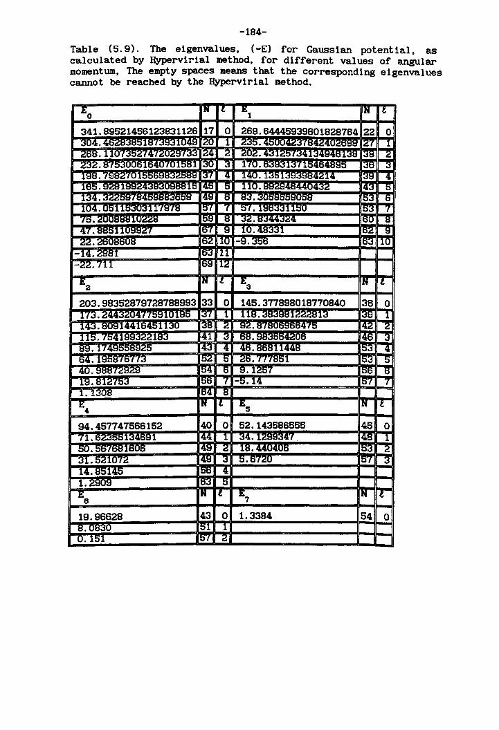
-184-
Table (5.9). The eigenvalues, (-E) for Gaussian potential, as calculated by Hypervirial method, for different values of angular momentum, The empty spaces means that the corresponding eigenvalues cannot be reached by the Hypervirial method.
EO IN It E1 IN ~
341.89521456123831126 17 0 269.64445939601828764 22 0 304. 4t;.....:H~iH~18·(J~~i049 20 1 235. 4~(If -1{H4~, IGf J. 268.11.07~~74·(~U~~f(~~ 24 _2 2U2. 431257341:<l4~4~ ~ _2 232. 875~OOfiI640"(OI~81 ;:IU ~ nl!.~;:Il;:1", l54B4H~5 I~O ~
198. (~ts~I\Jl 13"[ ~ L40·1351:-1~:-C~H4~~ ~ ~ 165.928IQ~~4 115 145 5 110. ~~. 14~2 [113 0 134.~~~Si-f7 149 ts J:f!.-==---......... D58 )~ ~ 104.05115303117978 I~·( "r ~.(. 196331150 10;:1 ".L 75. 11U228 159 8 32. R~44:4;'(4 ~ 8 47.88:)11~~J ItH _9 l.Q.483~1 [!i2 9 22. 269860J! 162 110 -9.356 l!);:I 10
-14.2981 163 111 -22.711 169 12
E2 IN It E3 IN It
203.98352879728788993 33 0 145.377898018770840 36 0 173. ~44~~04,T(591UI9~ 137 1 118.~lGGG81;:l ~ 1 143.809144IH4~ .J3Q 138 2 92.tsl i475 142 -~ 115.7541RR~~~183 141 ;:I ~. !lH ~ti ~ 89. 17.l1J 143 4 46.~~~ [!)~ 4
-64. 1958'(tst13 152 -~ 2D. ((Itsol ~ ~
40.988fG~G~ 154 6 9.12~1 Ltj6 ~ 19. 812·(~~ 10D J -0.14 l°.i ·f
1. 1308 164 8
Et IN It Ea IN It
94.457747566152 40 0 52.143586555 45 0 71. 1134691 144 1 34.1~~~47 148 1 5O.ot)(01:l1606 149 ~ ~.44ruulH ~3 _2 31. 521072_ 149 _3 J~._672Q ~"' _3 14.RH14S 156 11 1. 2909 63 5
Ee N t E7 IN t
19.96628 43 0 1.3384 54 0 8.08;:1U 51 1 0.151 ~"f _2
-185-
5.6 Eigenvalues of the hydrogen atom
The problem of the perturbed hydrogen atom has received
great attention in the last few years and has been attacked
by various approaches. Killingbeck [43,1977J attacked the
problem by using a non-perturbative finite difference method.
In a subsequent work Killingbeck and Galicia [44,1980J used
bypervirial relations together with the Hellmann-Feynman
theorem to get the energy coefficients of the energy
perturbation series. Lai and Lin [45,1981] applied the
Hypervirial-Pade framework to calculate the energy
eiaenvalues of various eiaenstates, Austin and Killingbeck
[46,1982] have used a renormalised series approach to compute
the energy levels of a perturbed hydroaen atom.
5.6.1 Power series approach
The power series approach to be discussed in this
section allows us to compute the energy eigenvalues for the
perturbed hydrogen atom. The power series approach is one of
the simplest and most accurate methods for calculating
ei,envalues. The Schrodinger equation for a system in which
the potential depends upon the distance r (spherically
symmetric potential ) is taken in our calculation to have the
form
( 5 • 82 )
where
(5.83 )
In (5.83) ~(r) is the radial wavefunction, which is
independent of the angles, and y{(e,~) is a spherical
-186-
harmonic, which is independent of r. If we insert equation
(5.83) into equation (5.82) and rearrange, we obtain the
radial equation
(5.84 )
where (t) is the angular momentum and <p( r) =r - 1R ( r). We can
express equation (5.84) with a new wavefunction R(r) as
(5.85)
where
t+1 R(r)=r ~(r) (5.86)
If we insert equation (5.86) into equation (5.85) we get
The wavefunction ~(r) can be expressed as
(5.88 )
For a perturbed hydrogen atom we take the potential VIr) as
- 1 V(r}=-r +).r (5.89)
If we substitute equations (5.88,5.89) in equation (5.87) we
obtain this recurrence relation after some algebra
[ n + 1 ) [n + 2 t+ 2 ] S ( n + 1 ) = 2 [ ( .t+ 1 + n ) 13- 1 ] r S ( n )
[ 2J 2 2 - 2B+f3 r S(n-l)+2).r S(n-2) (5.90)
where
(5.91)
To uae equation (5.90), S(O) i •• et equal to 1 tt') (hut
-187-
eigenvalues appropriate to the Dirichlet boundary conditions
'(~)=O. For a given (~) and two trial energies E1 and E2
, the
power series approach works out each 8(n) and the sum of the
8(n) at a specific r value, starting with S(0)=1 and
8(-1)=8(-2)=8(-3)=0. Although it takes a little while to find
an appropriate ~ value, there is usually quite a wide range
of ~ over which ,ood results can be obtained. If ~ is chosen
reasonably the series quickly conver,e and lead to two values
F(r,E1
) and F(r,E z )' from which an interpolated energy can be
found which would have ,iven F(r,E)=O. After a few
repetitions the ei,envalue corresponding to the boundary
condition '(r)=O is determined very accurately. For this
radial problem we cannot use the even parity of the
potential, because the coordinate range is from O~r~~.
5.6.2 Renormalised series approach
It has been shown by Killin,beck [14,1982) that the
hypervirial relations yield the perturbation series for the
ener,y E and for the expectation values <rn> for a hydrogen
atom with perturbation p.r), without the calculation of a
perturbed wave function. We also use the renormalised series
hypervirial approach for the perturbed hydrogen atom. The
radial 8chrodinger equation for this perturbed problem can be
written as
1 2 [ -1 1 2] "2DR(r)- r -~r - ~(.e.+l)r- R(r)=ER(r) (5.92 )
We write the potential ,iven in equation (5.92) as
-188-
-1 ( -1) V(r)=-Mr +A r-Kr (5.93 )
where
J.l= 1-AK (5.94)
We substitute the series expansions given by equations
(2.6,2.7) into the hypervirial relation (2.3) with
It(~+1), V =(M+AK), V1
= A. Collecting terms, we find 2 - 1
v = - 2
- (2 N + 1) [J.lA ( N -1 , M ) + KA ( N -1 , M - 1 ) ] + (2 N + 3 ) A ( N + 1 , M - 1 ) ( 5 • 95 )
The relation between the energy series and the A(N,M) series
is given as follows (from the Hellmann-Feynman theorem)
(M+ 1) B (M+ 1) =A ( 1, M) -KA ( -1, M) , (5.96)
The unperturbed eigenvalue is E(O) = -M2/2n
2for this case,
where n is the principal quantum number (1,2,3 .•. ). The
equations (5.95,5.96) suffice to calculate the full set of E
and A coefficients. We only need the value of E (0) gi ven
above and the starting term A(O,O) =1.
5.6.3 Finite difference approach
We use the finite difference method as a third method to
calculate the eigenvalues for the perturbed hydrogen atom.
The equation (5.87), after multiplying both side by r, takes
the form
(5.97)
To use the finite-difference method for this equation we make
-189-
the substitutions
2hD~(r)=~(r+h)-~(r-h) ( 5 . 98 )
2 2 h D ~(r)=~(r+h)+~(r-h)-2~(r) ( 5 .99 )
The equation (5.97) reduces to the form
[r+ (t+1)h ]~( r+h) + [r- (t+1 )hJ ~(r-h) =
2r~( r) +2rh 2 [V( r) -E] ~(r) (5.100 )
The next step is the introduction of a ratio variable R(r),
defined by the equation
where
~(r+h)=R(r)CP(r)
2 R(r)=l+h F(r)
(5.101)
(5.102)
With the substitution (5.101,5.102), the equation (5.100) is
converted to a recursive equation
[] [ ]F(r-h)
r+H F(r)= r-H R(r-h) + 2 [V (r) -EJ r (5.103)
Here H:(t+l)h is the only quantity which explicitly involves
the anaular momentum. If we start at r:H, then the first term
on the right vanishes, so we can arbitrarily set R=F=~:1 at
r:H-h without disturbing the rest of the calculation. The
rest of the paraphernalia (use of two E values etc) is as
before. By setting {:o we get the s-state solution, which is
-190-
appropriate to an odd solution for a one-dimensional problem.
By setting t=-l, with F(O)=~[V(O)-E], and starting at r=h we
get results appropriate to an even solution in one dimension.
The eigenvalue associated wi th strip width h is related to
the true eigenvalue by a perturbation-type expansion in h
2 4 E(h)=E+h E +h E --------2 ..
(5.104)
To get E we do the calculation using several different strip
widths, (h,2h,4h). The eigenvalues obtained are in error by a
f d h 2. leading term 0 or er We have applied a Richardson
extrapolation process to convert them to very accurate
2 4 results. To correct for the hand h error terms we use an
extrapolation formula given in the form
E=!5[64E(h)-20E(2h)+E(4h)] (5.105)
5.6.4 Results and discussion
The calculations reported here are for positive A, so
that well defined bound states exist, although quasi-bound
states exist when (A) is small and negative. We have used
three approaches to compute the energies eigenvalues for
various states and different values of perturbation parameter
A. Our main goal is to obtain accurate eigenvalues for this
problem and to compare the accuracy of the results as
obtained from the three approaches. The results are shown in
the table (5.10) and from these results it is clear that the
renormalised'series method works excellently at low values of
the perturbation parameter, where the series converges very
quickly and certainly leads to accurate eigenvalues
calculations. At A=O .1 the accuracy is to 20 signi ficant

-191-
digits, and in fact the accuracy of this technique is
crucially restricted by the choice to the value of the
renormalising constant k The rate of convergence is
sensitive to the value of k The finite difference and
power series methods work very well to compute the
eigenvalues, and their agreement is in general excellent. Our
confidence in the accuracy of the power series approach comes
from the following check; the computed eigenvalues are stable
wi th respect to changes in f3. We believe that the present
resul ts which have been calculated by the three approaches
are very good compared to those of other methods which have
been available for computing the eigenvalues for this
problem. We have used double precision arithmetic of 20
digits.
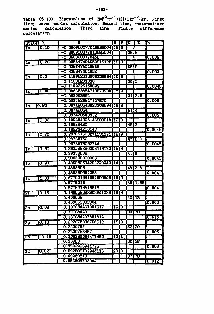
-192-
Table (5.10). Eigenvalues of H-p2_r -l+t (t+l)r-2+Ar, First Une; power series calculation; Second Une, renormaUsed series calculation; Third line, finite difference calculat ion.
IStatel A t; IR 113 IN -~ n rts 10.10 -0. '11 14 11::> ItI
-0. I I I Ill~RR"'O[l4 ~~ I~ -0. " (0456 10.005
rts 10.20 -0. 2356474C i151~~ ~ ~ -0. 23504'(1l ~ ~ -0.2356474fl4,",~)( 10.00J
rts 10.3 -0.1' 11 115 H -0.1' .1596 [;)0 I::> -0.1IB9~~6159693 10.0045
11S, 10.40 -0. i471.:nSl0934 115 IS -0. (JIIK~'1!\~'1"'S4 @! ~.~ -O.l ,7137870 10._005
11s 10.5U 0.OS'(1l ... n!'l4 116 IH O. m:r(47n"4 1::11 14 O. m:l14~n"4:.c,",:.c;.l 10.005
11s 10.60 O. 1QQ;.IH1l7n~1~ ,18 112 18 O. 1~~7.B4 .... () 146 13 0. IQ!oI .... H4;.1n'i146 IU.UU40
11s 10.70 O. "~/aof~~~~oJlltl~ Il~ I~ _0. "~fao(50 l!I 12.6 O.4:::tllts~IOU~"'44 10.0045
11s 10.80 O. 'lltH3U 110 ItI _0. ~, ~! ~ O. 10.0045
11s IU.90 O. 114 Its O. os 1Il~ 12.6 O. '~
10·oo!! 11s 11.00 0.577~1351961 ll~ ~
0.5T~!:3 lI,l::; 11. Ho O. 5T(m~5196~5 IU.UU~
12s 10.15 O.ll 'l I~ I~ ~ 0.46~ 40 1J O. III ~.~
13s 10.02 O. 1J'(nR441 '1HHloH 11t1 ,H 0.13'(nR44r _3t1 '(0
0.1J1U~440788!614 10.Ul0 [2p 10.10 O.~4:::"UfOtstsOfOObl~ 115 9
0.2220758 5~ ~u
O.~uf_~aof U.Uuo 2p I O.Jo 0.~"'R7! ,77485 ,15 8
O. 102 18 O. ""(5 10.000
[3d 10.02 O.U~"OUOf L.4,116 I?J! ~ 0.n~~'"'()ti13 137 10 O. 1 I III IU.Ul~
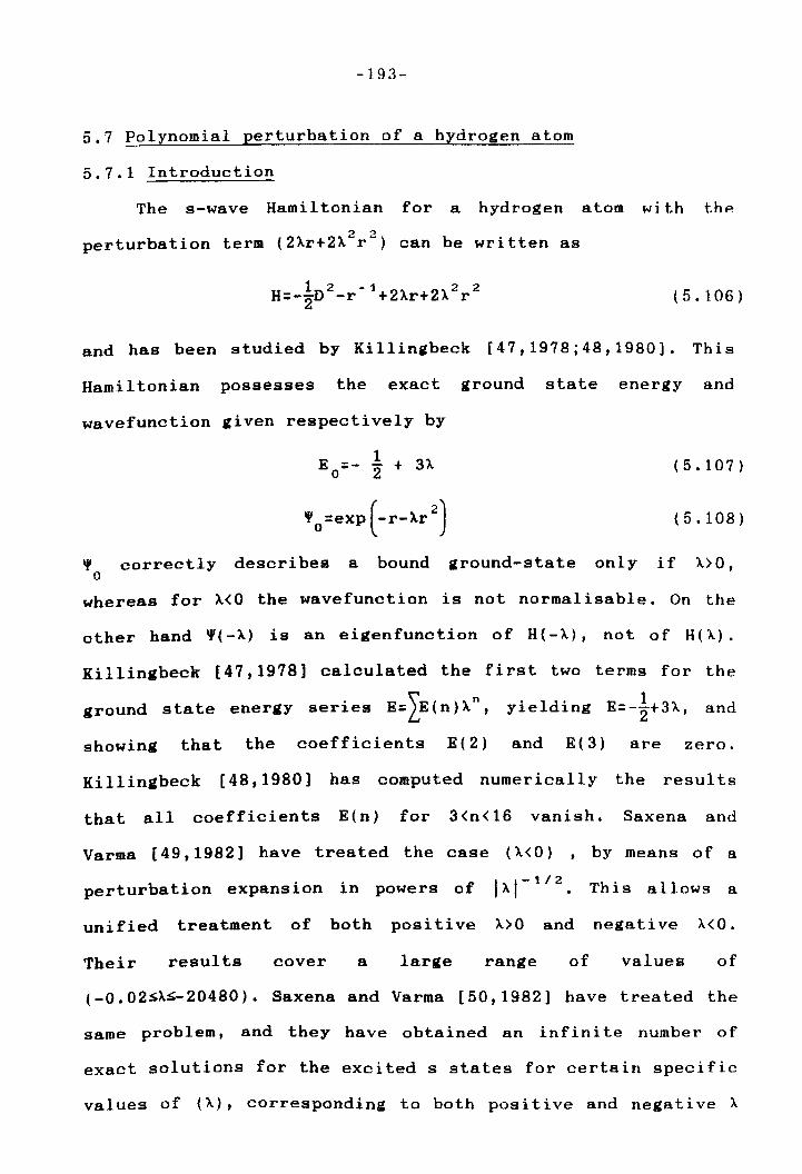
-193-
5.7 Polynomial perturbation of a hydrogen atom
5.7.1 Introduction
The s-wave Hamiltonian for a hydrogen atom wi th the
perturbation term (2Ar+2A2r2) can be written as
1 2 -1 2 2 H=-2D -r +2Ar+2A r (5.106)
and has been studied by Killinabeck [47,1978;48,1980]. This
Hamiltonian possesses the exact ground state energy and
wavefunction given respectively by
1 E =- - + 3A o 2
IV o=exp (-r-Ar 2)
(5.107)
(5.108 )
IV correctly describes a bound ground-state only if A>O, o
whereas for A<O the wavefunction is not normalisable. On the
other hand IV( -A) is an eigenfunction of H (- A), not of H ( A) .
Killingbeck [47,1978] calculated the first two terms for the
ground state energy series E=LE(n)An, yielding E=-~+3A, and
showing that the coefficients E(2) and E(3) are zero.
Killingbeck [48,1980] has computed numerically the resul ts
that all coefficients E(n) for 3<n<16 vanish. Saxena and
Varma [49,1982] have treated the case (A<O) , by means of a
t b t ' " f 1"1- 1/2• Thl'S allows a per ur a 10n expans10n 1.n powers 0 fI.
unified treatment of both positive A>O and negative A<O.
Their results cover a large range of values of
(-0.02~A~-20480). Saxena and Varma [50,1982] have treated the
same problem, and they have obtained an infini te number of
exact solutions for the excited s states for certain specific
values of (A), corresponding to both positive and negative A
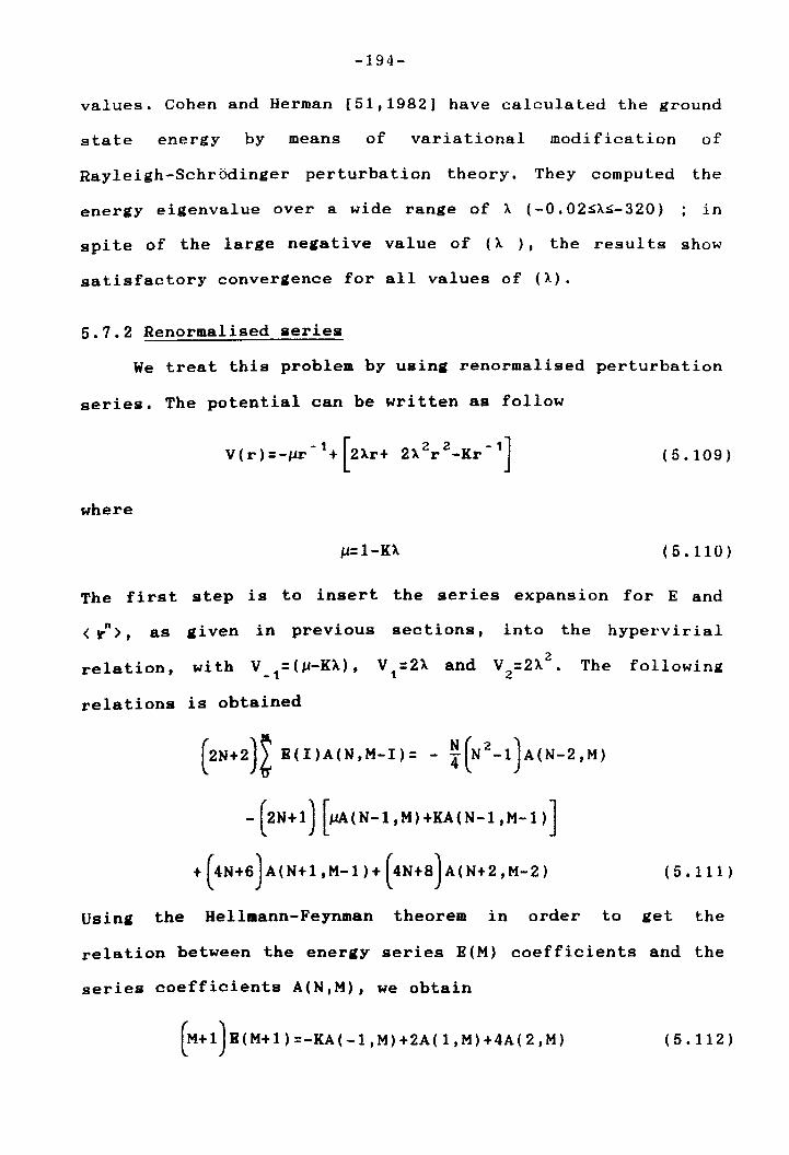
-194-
values. Cohen and Herman [51,1982] have calculated the ground
state energy by means of variational modification of
Rayleigh-Schrodinger perturbation theory. They computed the
energy eigenvalue over a wide range of A (-0. 02~>"~-320) ; in
spite of the large negative value of (>.. ), the results show
satisfactory convergence for all values of (A).
5.7.2 Renormalised series
We treat this problem by using renormalised perturbation
series. The potential can be written as follow
-1 [ 2 2 -1J V(r)=-~r + 2>..r+ 2A r -Kr (5.109)
where
~=1-KA (5.110)
The first step is to insert the series expansion for E and
< r n >, as given in previous sections, into the hypervirial
relation, wi th V _ 1 = (~-KA) , 2 V = 2 A and V = 2 A •
1 2 The following
relations is obtained
(2N+2)~ E(I)A(N,M-I)= - ~(N2_1)A(N-2,M)
- ( 2 N + 1) [#AA ( N -1 , M ) + KA ( N -1 , M - 1 ) ]
+ (4N+6 )A(N+1 ,M-1)+ (4N+8 )A(N+2 ,M-2) (5.111)
Using the Hellmann-Feynman theorem in order to get the
relation between the energy series E(M) coefficients and the
series coefficients A(N,M), we obtain
(M+1)E(M+1)=-KA(-1,M)+2A(1,M)+4A(2,M) (5.112)
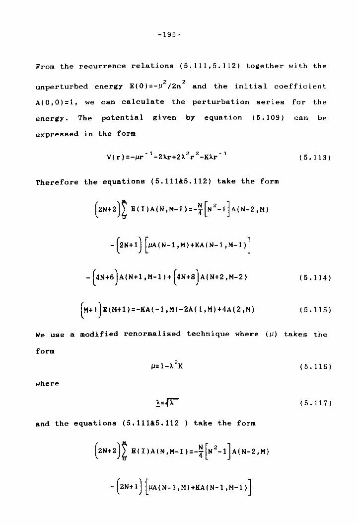
-195-
From the recurrence relations (5.111,5.112) together with the
2 2 unperturbed energy E (0) =-11 /2n and the ini tial coefficient
A(O,O)=l, we can calculate the perturbation series for the
energy. The potential given by equation (5.109) can be
expressed in the form
-1 22-1 V(r)=-l1r -2Ar+2A r -KAr (5.113)
Therefore the equations (5.111&5.112) take the form
- (2N+ 1) [1lA (N-l , M) +KA (N-1 , M-I) ]
- (4N+6 )A(N+l ,M-1)+ (4N+8 )A(N+2 ,M-2) (5.114)
(M+l)E(M+l)=-KA(-I,M)-2A(I,M)+4A(2,M)' (5.115)
We use a modified renormalised technique where (11) takes the
form
where
2 11= I-A K
and the equations (5.111&5.112 ) take the form
- ( 2 N + 1) [I1A ( N - 1 , M ) + KA ( N - 1 , M - 1 ) ]
(5.116)
(5.117)
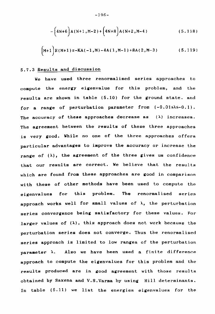
-196-
(5.118)
(M+1)E(M+1)=-KA(-1,M)-4A(1,M-1)+8A(2,M-3) (5.119)
5.7.3 Results and discussion
We have used three renormalised series approaches to
compute the energy eigenvalue for this problem, and the
results are shown in table (5.10) for the ground state. and
for a range of perturbation parameter from (-0.01$>"$-0.1).
The accuracy of these approaches decrease as (>..) increases.
The agreement between the results of these three approaches
is very good. Whi le no one of the three approaches offers
particular advantages to improve the accuracy or increase the
range of (>..), the agreement of the three gives us confidence
that our resul ts are correct. We believe that the resul ts
which are found from these approaches are good in comparison
wi th these of other methods have been used to compute the
eigenvalues for this problem. The renormalised series
approach works well for small values of A, the perturbation
series convergence being satisfactory for these values. For
larger values of (A), this approach does not work because the
perturbation series does not converge. Thus the renormalised
series approach is limited to low ranges of the perturbation
parameter A. Also we have been used a fini te difference
approach to compute the eigenvalues for this problem and the
resul ts produced are in good agreement wi th those resul ts
obtained by Saxena and V.S.Varma by using Hill determinants.
In table (5.11) we list the energies eigenvalues for the

-197-
range ( - 0 • 0 1 ~A~- 2 4 080 ) and compare them with numerical
computations of the ground state energy which were obtained
by Saxena.
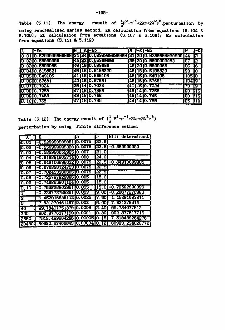
-198-
1 2 -1 2 2 Table (5.11). The energy result of ~ -r +2>'r+n r .perturbation by
using renor.allsed series .ethod. Ea calculation from equations (5.104 & 5.105); Eb calculatlon from equations (5.107 & 5. lOB); Ec calculation from equations (5.111 & 5.112)
1 2 -1 2 2 Table (5.12). The energy result of (- P -r +2Ar+2>' r ) 2
perturbation by using finite difference method.
-199-
5.8 The exponential cosine screened coulomb (ECSC) potential
The radial Schr6dinger equation for the exponential
cosine screened Coulomb (ECSC) potential is not solvable
analytically and can be expressed as
2 [ 1" - 2J D ~(r)+2 E+V(r) - ~(i+1)r ~(r)=O (5.120)
where
(5.121)
This potential is of importance in solid-state physics. It is
used in describing the potential between an ionized impurity
and an electron in a metal or a semiconductor . It has also
been used to represent the effective interaction between an
electron and a positronium atom in a solid. The (ECSC)
potential has been treated by several approximation methods.
Aparna and Pirtamp [52,1980] applied the generalized virial
theorem and Hellmann-Feynman theorem to calculate
perturbatively the bound state energy levels wi thout using
perturbed wavefunction. C.S.Lai [53,1982] has treated this
potential by using the hypervirial relations and the Pad(~
approximant E [10,10] and E [10,11] for different
eigenstates. In this section we set out to calculate the
bound-state energies of the ECSC potential for different
eigenstates, by applying the hypervirial and Hellmann-Feynman
theorems to calculate perturbatively the bound-state energy
levels without using perturbed wave functions. The ECSC
potential can be expanded in a power series of the screening
parameter by the Taylor expansion
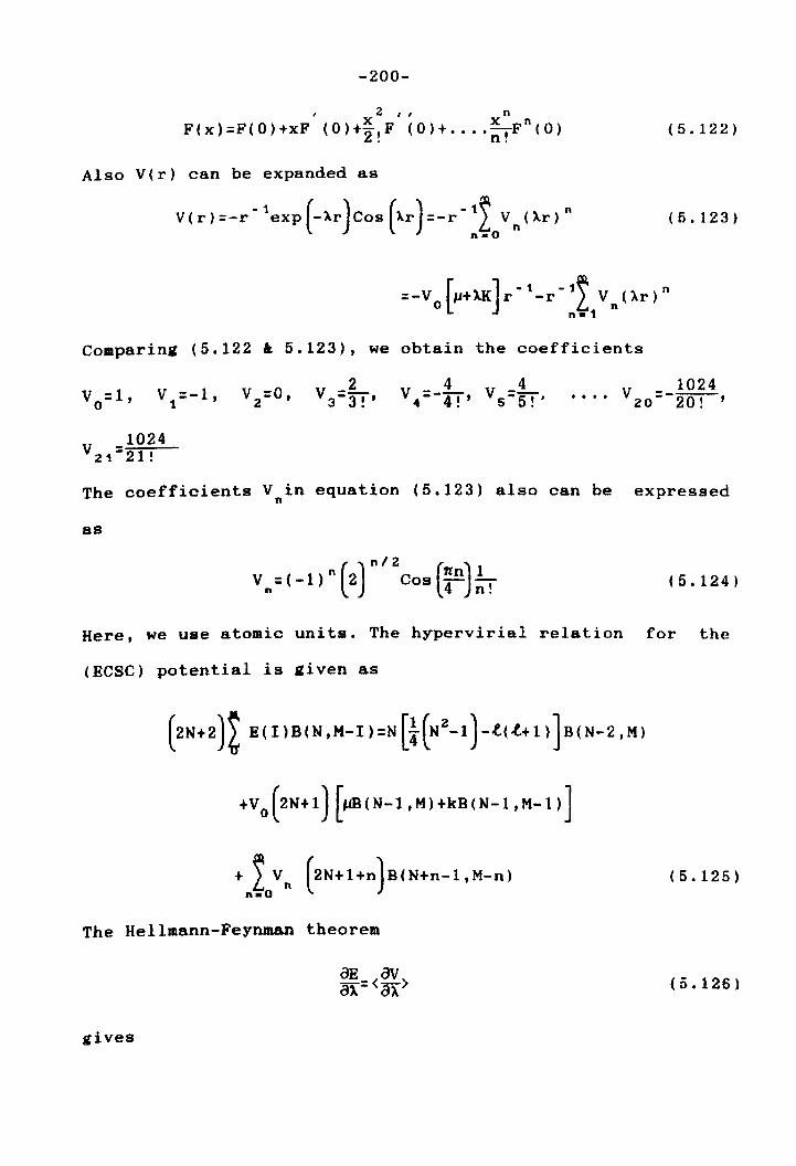
-200-
I 2 I' n X X n
F(x)=F(O)+xF (0)+2!F (O)+ .... nTF (0) (5.122)
Also V(r) can be expanded as
V ( r ) = - r -1 exp (-Xr ) Cos (Ar) = - r - 1! V n ( Xr ) n
n-O (5.123)
Comparing (5.122 & 5.123), we obtain the coefficients
V =1, o V =-1, 1
v =0, 2
1024 .•.. V20=-~'
The coefficients V in equation (5.123) also can be expressed n
as
V n = ( -1 ) n (2 ) n I 2 Cos (:n) ! ! (5.124)
Here, we use atomic units. The hypervirial relation for the
(ECSC) potential is given as
+V o(2N+1) [1lB(N-t ,M)+kB(N-1 ,M-1) ]
+ 2 Vn (2N+1+n)B(N+n-1,M-n) n.O
(5.125)
The Hellmann-Feynman theorem
(5.126)
gives
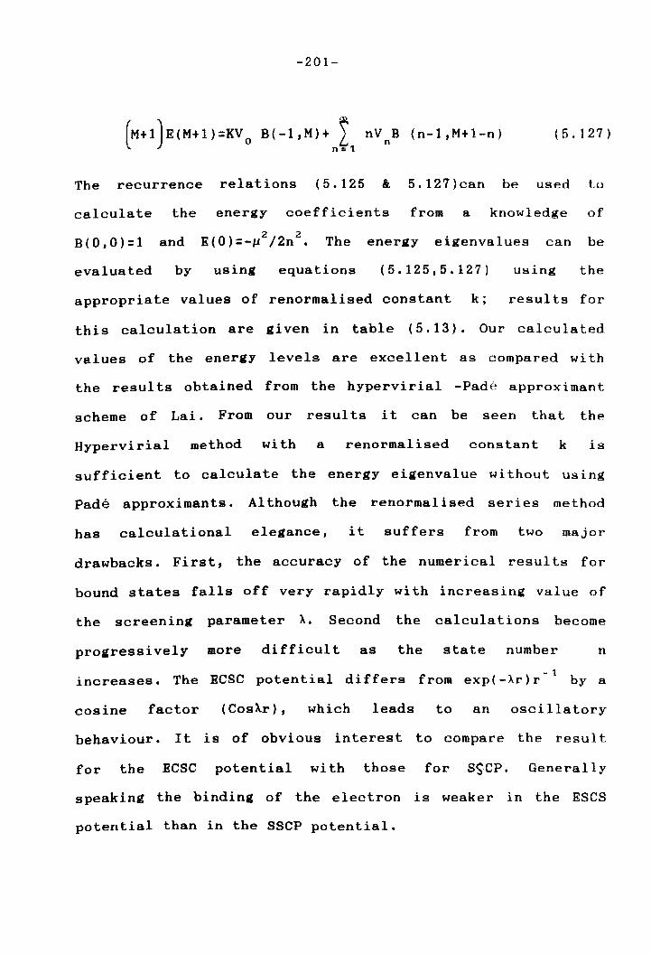
-201-
(M+1)E(M+1)=KV O B(-l,M)+ ~ nVnB (n-1,M+l-n) n,,1
(5.127)
The recurrence relations (5.125 & 5.127)can be used lo
calculate the energy coefficients from a knowledge of
B(O,O):l and
evaluated by
2 2 E(O)=-IJ /2n • The
using equations
energy eigenvalues can be
(5.125,5.127) using the
appropriate values of renormalised constant k; resul ts for
this calculation are given in table (5.13). Our calculated
values of the energy levels are excellent as compared wi th
the results obtained from the hypervirial -Pade approximant
scheme of Lai. From our resul ts it can be seen that the
Hypervirial method with a renormalised constant k is
sufficient to calculate the energy eigenvalue without using
Pade approximants. Al though the renormalised series method
has calculational elegance, it suffers from two major
drawbacks. First, the accuracy of the numerical results for
bound states falls off very rapidly with increasing value of
the screening parameter X-. Second the calculations become
progressively more difficult as the state number n
- 1 increases. The ECSC potential differs from exp( -X-r) r by a
cosine factor (CosX-r) , which leads to an oscillatory
behaviour. It is of obvious interest to compare the resul t
for the ECSC potential with those for SSCP. Generally
speaking the binding of the electron is weaker in the ESCS
potential than in the SSCP potential.
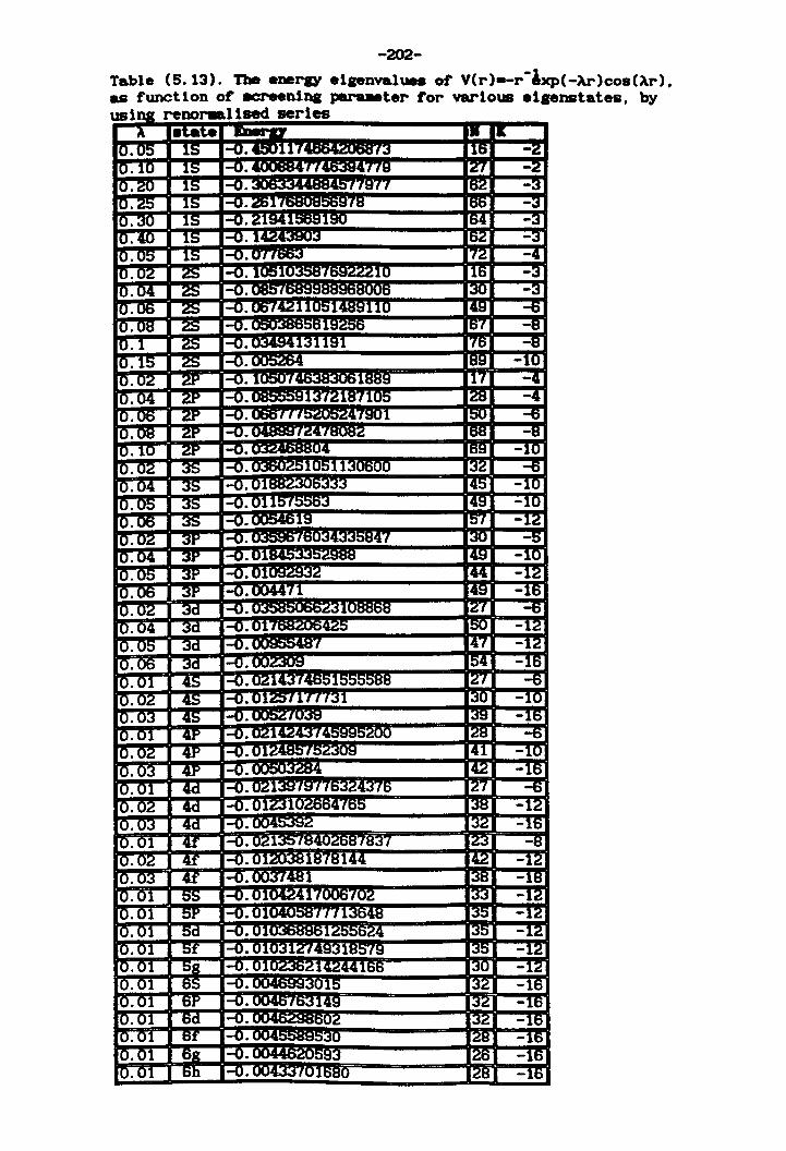
-202-
Table (6.13). The eDeraY eigenvalues of V(r)--r-ixp(-Ar)C08(Ar). as function of acreenlna para.eter for various elgenstates. by usi reno .... lised. series
-203-
5.9 Hulthen potential
The radial Schrbdinger equation for the Hulthen potential
can be written in atom units as
(5.128)
where
V H (r) :-Xexp (-xr ) [l-exp (-xr )] -1 (5.129)
where (X) is a screening parameter. The Hulthen potential at
small values of r behaves like a Coulomb potential, whereas
for large values of r it decreases exponentially, so that its
"capaci ty" for bound states is smaller than that of the
Coulomb potential. The energy levels always lie lower in the
Coulomb case than in the Hulthen case. The Hulthen potential,
apart from its ini tial interest in a number of areas of
physics ranging from nuclear physics (as a possible form of
nuclear interaction) to scattering theory to atomic physics,
has recently been shown to be a judicious choice of starting
point for the perturbation theoretic treatment of screened
Coulomb potentials. The Hulthen potential has been treated
numerically by Lai and Lin [54,1980], who appl ied the Pade
approximant technique to the analytic perturbation series
obtained through the use of hypervirial and Hellmann-Feynman
theorems. Also Dutt and Mukherji [55,1980] proposed a new
approximation scheme to obtain analytic expressions for the
bound-state energies and eigenfunctions for any arbitrary
bound (l,n) state of the Hulthen potential. The purpose of
-204-
this section is to study the bound-state eneraies of the
Hulthen potential for ~O. The Hulthen potential VH(r) in eq
(5.129) can be rewritten in the form
-tf' n =-r L V n (lr)
n.O (5.130)
where B
V = __ n_ n n! (5.131)
and Bn are the Bernoulli numbers. The Hulthen potential VH(r)
in equation (5.130) can be rewritten in another form
where
V (r)= -H
->..r Xe
lr/2+ -lr/2 = _ 2X [.....;;;;e-=--__ e_-=--_
Xr/2 -Xr/2 e - e
Coth(Z) 1 Z Z3 2Z5 2 2n = + --B Z2n-1 Z 3 - 45 + 945··+ 2n! 2n
where IZ/<i
(5.132)
(5.133)
Furthermore, we use the hypervirial relation as used in
previous sections, assuming that the eneraY' and the
M expectation values <r > can be expanded as
(5.134)
<r">=L B(M,N)l" (5.135)
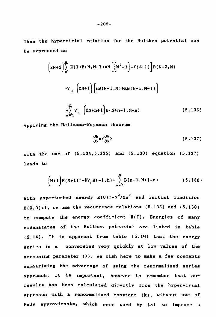
-205-
Then the hypervirial relation for the Hulthen potential can
be expressed as
-v 0 (2N+1) [1JB(N-1 ,M) +KB( N-1 ,M-1 )]
(5.136)
Applyin~ the Hellmann-Feynman theorem
(5.137)
with the use of (5.134,5.135) and (5.130) equation (5.137)
leads to
(M+1)B(M+l)=-KVOB(-1,M)+ 2 B(n-l,M+l-n)
~ n-1
(5.138)
With unperturbed ener~y &(0)=_,.,2/ 2n 2 and initial condition
B(0,0)=1, we use the recurrence relations (5.136) and (5.138)
to compute the energy coefficient E( I). Eneraies of many
eiaenstates of the Hulthen pote£"'ltial are listed in table
(5.14). It is apparent from table (5.14) that the eneray
series is a convergina very quickly at low values of the
screenina parameter (A). We wish here to make a few comments
summarisinar the advanta~e of using the renormalised series
approach. It is important, however to remember that our
results has been calculated directly from the hypervirial
approach with a renormalised constant (k), wi thout use of
Pade approximants, which were used by Lai to improve a
-206-
convergent series. It is necessary to point out that the
agreement of our
results of Lai is
calculated
good. The
energy eigenvalues
renormalised series
with the
approach
works very well even for higher excited states with higher
value of angular momentum. We believe that the accuracy of
our results may be improved even further with a better choice
of renoraalised constant k, the approach gives well converged
eigenvalues for the best values of the renormalised constant
k.
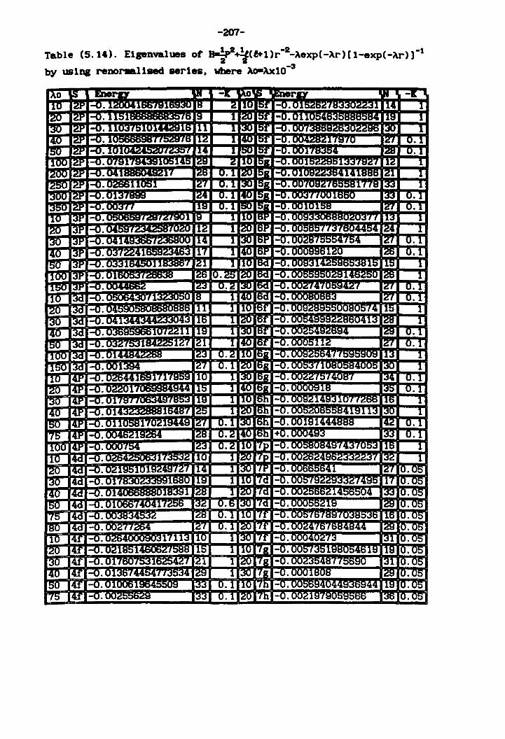
-207-
Table (5.14). Elsenvalues of ~2~(t+Ur-2-Aexp(-Ar)(l-exp(-Ar»)-1 by uslna renor.allsed aerlea. where Ao-Axl0-3

-208-
Table (5.14 continued)
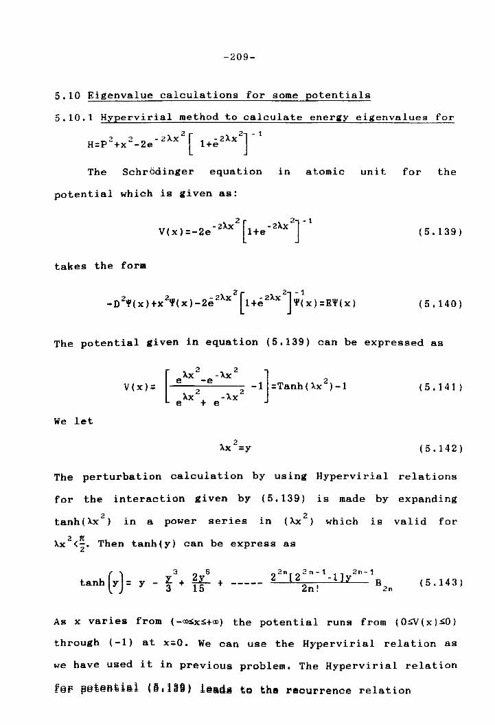
-209-
5.10 Eigenvalue calculations for some potentials
5.10.1 Hypervirial method to calculate energy eigenvalues for
H=p2+x2_2e - 2AX2 [ 1+e2AX2]-1
The Schrbdinger equation in atomic unit for the
potential which is given as:
V(x)=_2e- 2AX 1+e- 2AX 2[ 2]-1 (5.139)
takes the form
2 2 - 2AX - lAX 2[ 2]-1 -D '(x)+x '(x)-2e l+e '(x)=E'(x) (5.140)
The potential given in equation (5.139) can be expressed as
(5.141)
We let
2 AX =y (5.142)
The perturbation calculation by using Hypervirial relations
for the interaction given by (5.139) is made by expanding
2 2 tanh(Xx) in a power series in (AX ) which is valid for
2 re AX <2' Then tanh(y) can be express as
() ¥..3+ ~ 22n[22n-1_1]y2n-1B
tanh y = y - 3 15 + ----- 2n! 2n (5.143)
As x varies from (-~x~+oo) the potential runs from (O~(x)~O)
through (-1) at x=O. We can use the Hypervirial relation as
we have used it in previous problem. The Hypervirial relation
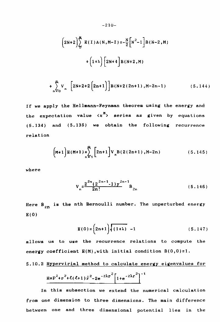
-210-
+ ~ Vn [2N+2+2(2n+1)]B(N+2(2n+1),M-2n-1) n=O
(5.144)
If we apply the Hellmann-Feynman theorem using the energy and
the expectation value <x M) series as given by equations
(5.134) and (5.135) we obtain the following recurrence
relation
(5.145)
where
22n(22n-1_1) 2n-1 V = Y B
n 2n! 2n (5.146)
Here B is the nth Bernoulli number. The unperturbed energy 2n
E(O)
(5.147)
allows us to use the recurrence relations to compute the
energy coefficient E(M),with initial condition B(0,0)=1.
5.10.2 Hypervirial method to calculate energy eigenvalues for
In this subsection we extend the numerical calculation
from one dimension to three dimensions. The main difference
between one and three dimensional potential lies in the
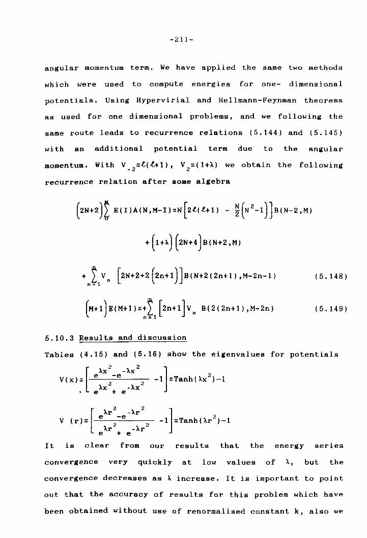
-211-
angular momentum term. We have applied the same two methods
which were used to compute energies for one- dimensional
potentials. Using Hypervirial and Hellmann-Feynman theorems
as used for one dimensional problems, and we following the
same route leads to recurrence relations (5.144) and (5.145)
with an additional potential term due to the angular
momentum. With V =.t(.t+1), V =(1+A) -2 2
we obtain the following
recurrence relation after some algebra
(5.148)
(5.149)
5.10.3 Results and discussion
Tables (4.15) and (5.16) show the eigenvalues for potentials
[
2 2 Xx -Xx e -e
V(x)= ? 2 Xx~ -Xx
• e + e
It is clear from our results that the energy series
convergence very quickly at low values of X, but the
convergence decreases as X increase. It is important to point
out that the accuracy of results for this problem which have
been obtained without use of renormalised constant k, also we
-212-
used the Pade approximants as second method to compute the
energy eigenvalue. The agreement between the two methods are
very good for low values of A, but for high values of A the
Pade approximants give more accurate eigenvalues. We have
computed many energy eigenvalues of the potential given by
equation (5.141), for different values of (0. 0 1~A~0. 1) and
for the ground and first four
results for this calculation
excited state. We list
for
our
in table (5.15) one
dimension
different
and in
values
table (5.16) for
of (0. 0 l~ASO. 05) ,
(t=O,2,5,lO) and state number n.
three dimensions, for
different values of
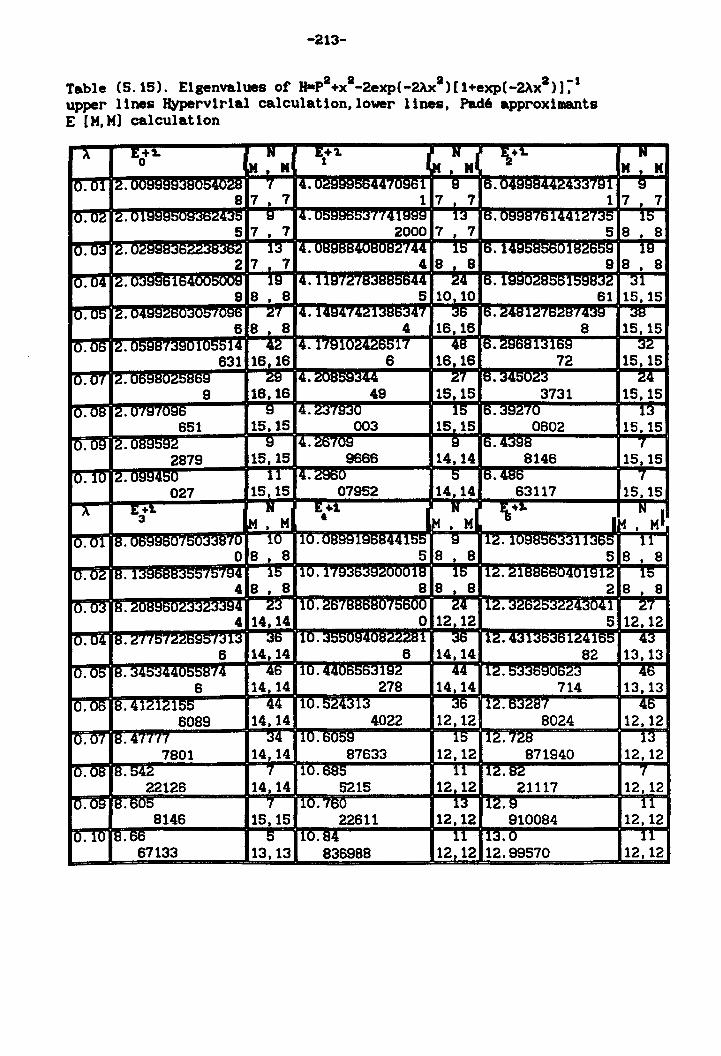
-213-
Table (5.15). £lgenvalues of H-p2+xa_2exp(-2Axa)[1+exp(-2Axa)]~1 upper lines Hypervlrlal calculation, lower lines, Pad, approxlmants £ [M,M] calculation
A 1:,+2- N 1:.+'2. N ~ \+1. 0 .. , M 1 M , M
[0.01 ,2. nnQQQ~ "<I~n"'4fl7N 7 4. ,70961 8 ,6,( L74~~791
8 7 • 7 17, 7 1 10. 02 !2. 01~ :~!'i 9 4. n"'QQR"'"<I7741999 13 6. Utlll:tts lo1441iff;J::;
5 7 , 7 2000 7 , 7 5 10.03 I~· i~ 13 4.n~8RR41 ;(44 15 6.1 Jl
2 7 , 7 4 8 , 8 9 10.04 i~· ilR41 1~ 4. 1 U:H4:: 1 ./1 24 6. 1~ il"'Q~·<l7
9 8 , 8 5 10,10 61 10. 05 i2.n4' "U~O '2:1 4.1494742' ,-I 3D D. 24B1e:: Ib4::tH439
6 8 , 8 4 16 16 8 0.06 ~. U::;~tfl39010titi14 42 4. r/911 747R"il-1 48 16. 28681310~
631 16,16 6 16,16 72 "0.07 2. ~~ 4. 27 16 • ~4Rn7~
9 16,16 49 15,15 3731 O.OB 2.uI~lu~o 9 4 . .G.:sI~.:su 15 6 . .:stll.Glu
651 15,15 003 15,15 0602 "0.09 2. 9 4.26709 9 6.4398
2879 15,15 9666 14,14 8146 0.10 2. rlQ~4Rr 11 4.~960 5 6.4B6
027 15,15 07952 14,14 63117
N M , M
9 7 , 7
15 8 , 8
18 8 , 8
31 15,15 3B
15,15 3~
15,15 24
15,15 13
15,15 7
15,15 7
15,15 A E,+2. It E,+1 I M ,N M
\u. I ~ ,N HI 3 H , H
, 0.01 B. ItiU;j;jtsIU lU 10.UB99 m:iti ~ 12.1 111365 11
0 8 , 8 5 8 , 8 5 8 , 8 "0.02 B. IIo/tll4 15 10.1'1 IlIB 15 12.21: 14[11912 15
4 8 , 8 8 8 , 8 2 8 , 8 0.03 B.7f 23 .10. 4::b 1 ____ -' 100UU 24 . 12. :~~H~~~774~na,1 27
4 14,14 0 12.12 5 12,12 0.04 B.4::IIOI IIJ13 3D 110. 11 36 112. 4313D30124165 43
6 14,14 6 14,14 82 13,13 0.05 B. '~4R~44I1RRR7 4 46 10.44nRRR~192 44 ,l~. 40
6 14,14 278 14,14 714 13,13 0.06 8.41212155 44 10.524313 36 i12.63287 46
6089 14,14 4022 12,12 8024 12,12 0.07 8.47777 34 110.6059 15 112. 728 13
7801 14,14 87633 12,12 871940 12,12 0.08 B.542 7 110.oB5 11 12.B2 7
22126 14,14 5215 12,12 21117 12,12 0.09 B.605 7 110.760 13 12.9 11
8146 15,15 22611 12,12 910084 12,12 0.10 18.66 5 110.84 11 113•0 11
67133 13,13 836988 12,12 12.99570 12,12
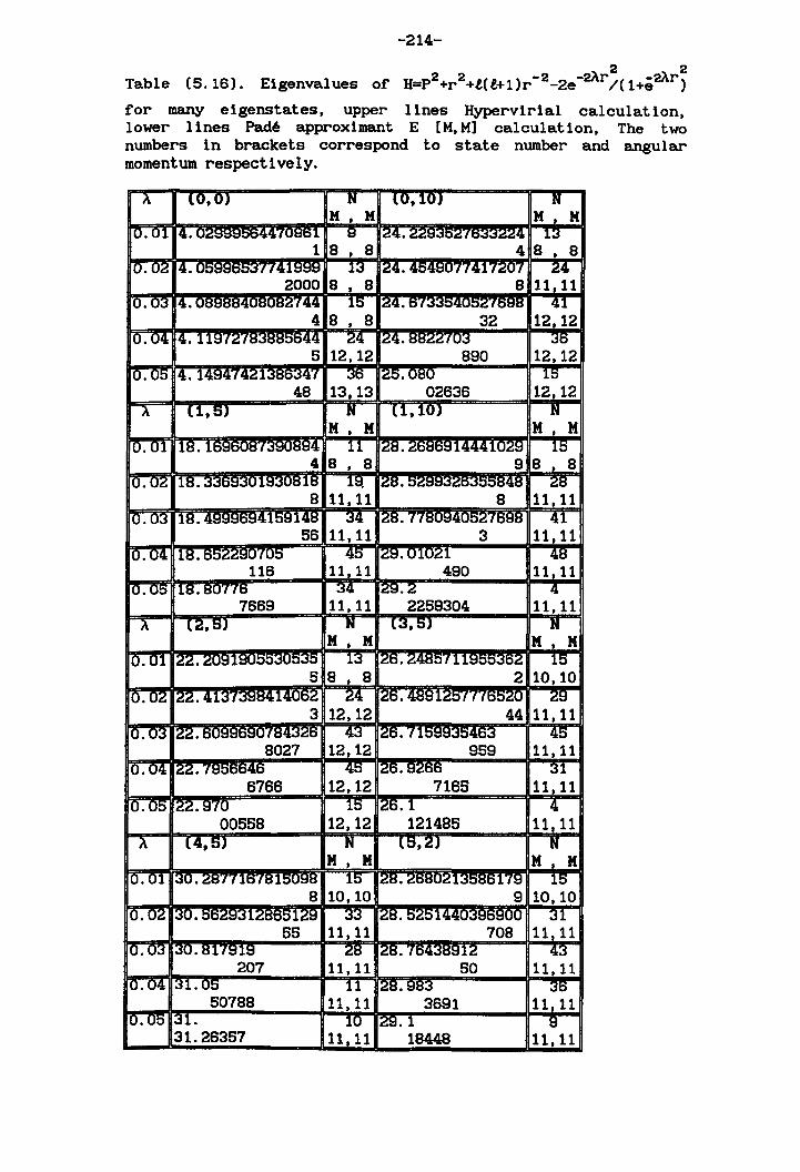
-214-
2 2 Table (5.16). Eigenvalues of' H=p2+r 2+t (t+1)r -2_2e -2Ar /( 1+e2~r)
f'or many eigenstates, upper lines Hypervirial calculation, lower lines Padl: approximant E [M, M] calculation, The two numbers in brackets correspond to state number and angular momentum respectively.
A (0,0) N (0,10) N M , M M , M
10 . 01 14. ,70S61 S 1~4. if !4 13 18, 8 4 8 , 8
10.02 14. 1/141888 13 124.45480',,41720', 24 2000 8 , 8 8 11,11
10.03 4. ;f44 15 124•cf :/tnns 41 4 8 , 8 32 12,12
0.04 14. 1ll::H~1 :il -- 24 i24. tsts~~ IU;j ~o
5 12,12 890 12,12 j(Y.-05 14. 1484742' ,7 36 125.0BO 10
48 13,13 02636 12,12 A (1,5) N U,lO) N
M , M M , M [0.01 118. , I1 nR~4 11 12B.26B6814441028 10
4 8 , 8 9 8 , 8 10.02 IUS. Il830BIB 18. 12B . 2B
8 11,11 8 11,11 10.03 118. blo~148 34 128. 778(1~4 ifCl:JO 41
56 11,11 3 11,11 [0.-04 lIB. !(Ut) 45 128. UIU21 4B
116 11,11 490 11,11 rc·05 118.80776 34 128 . 2 4
7669 11,11 2259304 11,11 A (2,5) N l3,5) N
M , M M , M 10. 01 122.208 11!'i:i!'i 13 126. 24B571' 15
5 8 , 8 2 10,10
10. 02 122.41"'''l:Jo~14062 24 IZ6. 4B81Z5', 1 (OO~U Z8 3 12,12 44 11,11
10.03 122 . 11 !.lL";l7R 43 26. 'f Fn 45 8027 12,12 959 11,11
10.04 122 • 1 i4ti 45 26.8266 31 6766 12,12 7165 11,11
10.05 22. 8~(0 15 26.1 4 00558 12,12 121485 11,11
A l4,5) N (5,2) N M , M M , M
1).01 30. 287716'fBloU8B 15 128. 268021~t)Bol'f8 15 8 10,10 9 10,10
U.02 130• I1ZB651Z8 33 12B. 02ti 144l '.iHhHLJl ~1
55 11,11 708 11--,-11 U.03 130. Bl'f81S 2B 12B. "04:-i~81Z 43
207 11,11 50 11,11 10.04 131. 05 11 12B.8B3 36
50788 11,11 3691 11,11 10.05 1~1. 10 128 . 1 8
31.26357 11.11 18448 11.11
-215-
CONCLUSION
In the preceding chapters of this work we have seen,
wi thout being concerned wi th any specific application, how
perturbation and non-perturbation methods can be used for
solving the eigenvalue problem. The numerical methods
presented in this work have been tested for Schrodinger
equation involving several perturbed and unperturbed
potentials. These methods have been shown to be very
effective and to be more simple and accurate than the widely
used matrix calculations. We would like to emphasize the
following aspects of the present eigenvalue calculations:.
1.The methods which have been used all yielded highly
accurate results. These results showed good agreement wi th
each other or with those (when available) in the literature.
Our methods proved to be very effective in dealing with one,
two, three and N dimensional radial problems.
2.It is interesting to note that the renormalised series
method can be extended to compute the energy eigenvalues fol'
quasi-bound states of potentials such as
1.
I!.
2 3 V(x)=x +>"x
2 5 V(x)=x +>"x
The renormalised series converge well for sufficiently small
values of >...
3.We studied a double well potential Z 2 2N V(x)=-Z X +x , for'
various values of 2N, Z2 and state number n, by using
perturbative and non-perturbative methods. All methods
yielded highly accurate results except that the renormali
-216-
series gave poor accuracy at low values
works very well for high values of Z2.
2 of Z , al though it
4.It has been shown, (section 2.4), that expectation values
such as <x 2N) can be calculated without storing explicit
values of the wavefunction ,. The relevant difference
equation
involves the use of energy calculations, which can be
performed by Jlany methods (e.g renormalised series, finite
difference and power series). In numerical work one or more
fini te values of £ are used to estimate the value of the
limit. For double precision calculations, we found that
·8 £:10 gives reasonably accurate results.
5.In the case of perturbation methods (both hypervirial and
inner product) we have shown how one may avoid divergence
problem, by using the renormalising constant k and (when
necessary) Pade approximants and the Aitken procedure.
6.In the present work, we have compared various methods, with
respect to their accuracy and divergence properties and
changing behaviour with respect to variation of
I.perturbation parameters (e.g A,g,a).
II.state number n.
11 . d (x2N) I .power l.n ex of a perturbing potential.
It is worth pointing out that perturbation methods are
sensi tive to points (I,ll, Ill), but nonperturbation method:~
-217-
222 series method in the case Y=~x /(1+ax ) requires ax (1).
7. Our results allow us to study the nUllerical behaviour of
eneray levels for the potentials
2 211 I. #.IX +~ , ,.,=0,1; 2N=4,6,8 •••• 18,20
2 XX 211
11. Y(x)=x + 2 ;2N=4,6,8 •••• 18,20 l+ax
for different index 2N, perturbation parameters X&a and state
nuaber n. We have seen how the order of the eneray levels
varies with these parameters. We determined the value of ~ at
which a crossina point occurs for potential (I) (i.e ~5).
8.In chapter four we investiaated the eiaenvalue problem
211
I. :t 1 2 ax
Y (x)='2 x :t =--1+ aa:x 2
;2N=4,6
11.
We have not observed any fundamental difference in behaviour
between the Y- and y+ cases as we vary the perturbation
parameters (oc, a ) and index ( 2N ). We used (aoc) and (a) as
perturbation parameters.
9.We have discovered that the renorllallsed series method does
not work so well for the perturbed potential
2 2N 2 I.Y=#.IX +X(x -Xx ); lJ=l+XK; 2N=6,8
and aives reduced accuracy. However, we partly overcame this
difficulty by introduoina hiaher power. of X
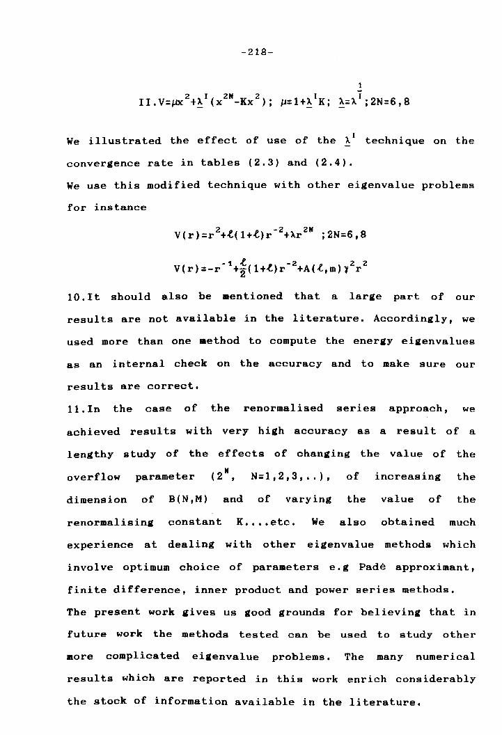
-218-
1
2 I 2" 2 I I II.V=~ t~ (X -Kx ); ~=lt~ K; ~=A ;2N=6,8
We illustrated the effect of use of the AI technique on the
convergence rate in tables (2.3) and (2.4).
We use this modified technique with other eigenvalue problems
for instance
2 -2 2N V(r)=r t~(lt~)r tAr ;2N=6,8
-1 ~ , -2 9 2 2 V(r)=-r t"2(lt'\.)r tA(""m)l r
10. It should also be mentioned that a large part of our
results are not available in the literature. Accordingly, we
used more than one method to compute the energy eigenvalues
as an internal check on the accuracy and to make sure our
results are correct.
11.In the case of the renormalised series approach, we
achieved results with very high accuracy as a result of a
lengthy study of the effects of changing the value of the
overflow parameter (2", N=1,2,3, •• ), of increasing the
dimension of B(N,M) and of varying the value of the
renormalising constant K •.•• etc. We also obtained much
experience at dealing with other eigenvalue methods which
invol ve optimum choice of parameters e. g Pade approximant,
finite difference, inner product and power series methods.
The present work gives us good grounds for believing that in
future work the methods tested can be used to study other
more complicated eigenvalue problems. The many numerical
results which are reported in this work enrich considerably
the stock of information available in the literature.
-219-
REFERENCES
1. C.M. Bender and T.T. Wu, Phys. Rev. 184(1968)1231.
2. B. Simon, Ann. Phys. 58(1970)76.
3. S.N. Biswas, et. aI, J. Math. Phys. 14(1973)1190.
4. K. Banerjee, Proc. Roy. Seo. A364(1978)265.
5. J.E. Drumaond, J. Phys. A: Math. Gen. 14(1981)1651.
6. J.E. Drummond, J. Phys. A: Math. Gen. 15(1982)2321.
7. G. Sehiffner and D. Stanzial, Nuovo Cimento. 90B(1985)74.
8. J.P. Killinabeck, Phys. Lett. 65A(1977)87.
9. J.P. Killinabeck, J. Phys. A: Math. Gen. 13(1980)L35.
10. J.P. Killinabeck, J. Phys. A: Math. Gen. 13(1980)49.
11. J.P. Killinabeck, J. Phys. A: Math.Gen 14(1980)1005.
12. J.P. Killingbeck, Microcomputer Quantum Mechanics (1982).
13. J.P. Killinabeek, et. aI, J. Phys. A: Math. Gen. 18(1980)793.
14. J.P. Killinabeek, Rep. Prog. Phys. 48(1985)53.
15. J.P. Killinabeek, J. Phys. A: Math. Gen. 20(1987)601.
16. J.P. Killinabeek, J. Phys. A: Math. Gen. 20(1987)1411.
17. R. Balsa, et. aI, Phys. Rev. D28(1983)1945.
18. R.M. Quick and H.G. Miller, Comment (1984).
19. F.T Bioe, et. aI, Phys. Rep. 43(1978)305.
20. Nasit. Ari and Metin. Demiralp, J. Math. Phys. 26(1985)1179.
21. J.P. Killingbeek and M.N. Jone, J. Phys. A: Math. Gen
19(1986)705.
22. J.P. Killinabeck , J. Phys. A: Math. Gen. 18(1985)LI025.
23. A.K. Mitra, J. Math. Phys. 19(1978)2018.
24. S. Galieia and J. Killinabeck, J. Phys. Lett. A71(1979)17.
25. R.S. Kaushal, J. Phys. A: Math. Gen. 12(1979)L253.
26. N. Bessis and G. Bessis, J. Math. Phys. 21(1980)2780.
27. A. Hautot, J. Comp. Phys. 39(1981)72.
28. C.S. Lai and H.E. Lin, J. Phys. A: Math. Gen. 16(1982)1495.
-220-
29. V.Fack and G.V.Berghe, J. Phys. A: Math. Gen. 18(1985)3355.
30. G. Auberson, Commun. Math. Phys. 84(1982)531.
31. G. Auberson and T. Boissiere, Nuovo.Cimento. 75B(1983)105.
32. H.C. Praddaude, Phys. Rev. A6(1972)1321.
33. J.P. Killingbeck, J. Phys. B: At. Mol. Phys. 14(1981)L461.
34. J.A.C. Gallas, Phys. Rev. A29(1984)132.
35. J.P Killingbeck , J. Phys. A: Math. Gen. 18(1985)245.
36. J.P. Killingbeck, J. Phys. B: At. Mol. Phys. 20(1987)5387.
37. M.Grant and C.S. Lai, Phys. Rev. A20(1979)718.
38. C.S. Lai, Phys. Rev. A23(1981)455.
39. B.R. Vrscay, Phys. Rev. A33(1986)1433.
40. N. Bessis, et. aI, J. Phys. A: Math. Gen. 15(1982)3679.
41. C.S. Lai, J. Phys. A: Math. Gen. 16(1983)L181.
42. A. Chatterjee, J. Phys. A: Math. Gen. 18(1985)2403.
43. J.P. Killingbeck, J. Phys. A: Math. Gen. 10(1977)L99.
44. J.P. Killingbeck and S. Galicia, J. Phys. A: Math. Gen.
13(1980)3419.
45. C.S. Lai and W.C. Lin, Can. J. Phys. 59(1981)733.
46. B.J. Austin and J.P. Killingbeck, J. Phys. A: Math. Gen.
18(1982)L443.
47. J.P. Killingbeck, Phys. Lett. 67A(1978)13.
48. J.P. Killingbeck, J. Phys. A: Math. Gen. 13(1980)L393.
49. R.P. Saxena and V.S. Varma, J. Phys. A: Math. Gen.
15( 1982)L221.
50. R.P. Saxena and V.S. Varma, J. Phys. A: Math. Gen.
15(1982)L149.
51. M. Cohen and G. Herman, J. Phys. A: Hath. Gen. 16(1983)4025.
52. Aparna. Ray and Pirtam.P. Ray, Phys. Lett. 83A(1981)383.
53. C. S. Lai, Phys. Rev. A26(1982)2245.

-221-
54. C.S. Lai and W.C. Lin, Phys. Lett. 78A(1980)335.
55. R. Dutt and U. Mukherji, Phys. Lett. 90A(1982)396.
56. G.A.Jr. Baker, Bssentials of Pade approximants,
Academic press (1976).