Embed Size (px)
Citation preview

UNIVERZA NA PRIMORSKEM
FAKULTETA ZA MATEMATIKO, NARAVOSLOVJE IN
INFORMACIJSKE TEHNOLOGIJE
Master’s Thesis
(Magistrsko delo)
The University Timetabling Problem – Complexity and an
Integer Linear Programming Formulation: a Case Study of
UP FAMNIT
(Problem urnika na univerzi – racunska zahtevnost in formulacija s celostevilskim
linearnim programom: studija primera UP FAMNIT)
Ime in priimek: Nevena Mitrovic
Studijski program: Matematicne znanosti
Mentor: izr. prof. dr. Martin Milanic
Somentor: doc. dr. Jernej Vicic
Koper, september 2017
Mitrovic N. The UP FAMNIT Timetabling Problem – Complexity and an ILP Formulation.
Univerza na Primorskem, Fakulteta za matematiko, naravoslovje in informacijske tehnologije, 2017 II
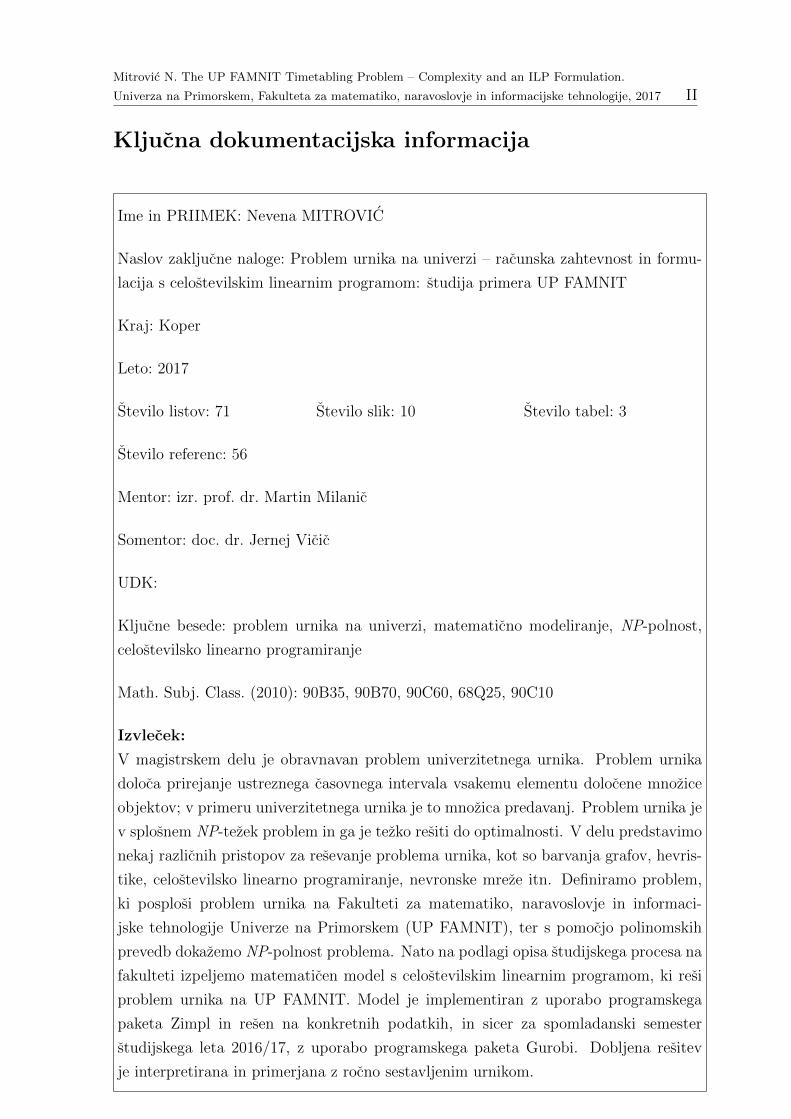
Kljucna dokumentacijska informacija
Ime in PRIIMEK: Nevena MITROVIC
Naslov zakljucne naloge: Problem urnika na univerzi – racunska zahtevnost in formu-
lacija s celostevilskim linearnim programom: studija primera UP FAMNIT
Kraj: Koper
Leto: 2017
Stevilo listov: 71 Stevilo slik: 10 Stevilo tabel: 3
Stevilo referenc: 56
Mentor: izr. prof. dr. Martin Milanic
Somentor: doc. dr. Jernej Vicic
UDK:
Kljucne besede: problem urnika na univerzi, matematicno modeliranje, NP-polnost,
celostevilsko linearno programiranje
Math. Subj. Class. (2010): 90B35, 90B70, 90C60, 68Q25, 90C10
Izvlecek:
V magistrskem delu je obravnavan problem univerzitetnega urnika. Problem urnika
doloca prirejanje ustreznega casovnega intervala vsakemu elementu dolocene mnozice
objektov; v primeru univerzitetnega urnika je to mnozica predavanj. Problem urnika je
v splosnem NP-tezek problem in ga je tezko resiti do optimalnosti. V delu predstavimo
nekaj razlicnih pristopov za resevanje problema urnika, kot so barvanja grafov, hevris-
tike, celostevilsko linearno programiranje, nevronske mreze itn. Definiramo problem,
ki posplosi problem urnika na Fakulteti za matematiko, naravoslovje in informaci-
jske tehnologije Univerze na Primorskem (UP FAMNIT), ter s pomocjo polinomskih
prevedb dokazemo NP-polnost problema. Nato na podlagi opisa studijskega procesa na
fakulteti izpeljemo matematicen model s celostevilskim linearnim programom, ki resi
problem urnika na UP FAMNIT. Model je implementiran z uporabo programskega
paketa Zimpl in resen na konkretnih podatkih, in sicer za spomladanski semester
studijskega leta 2016/17, z uporabo programskega paketa Gurobi. Dobljena resitev
je interpretirana in primerjana z rocno sestavljenim urnikom.
Mitrovic N. The UP FAMNIT Timetabling Problem – Complexity and an ILP Formulation.
Univerza na Primorskem, Fakulteta za matematiko, naravoslovje in informacijske tehnologije, 2017 III
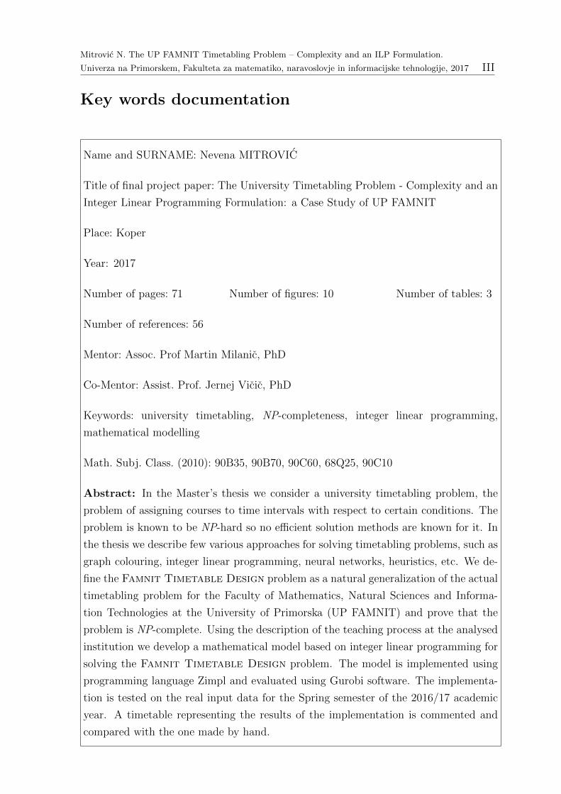
Key words documentation
Name and SURNAME: Nevena MITROVIC
Title of final project paper: The University Timetabling Problem - Complexity and an
Integer Linear Programming Formulation: a Case Study of UP FAMNIT
Place: Koper
Year: 2017
Number of pages: 71 Number of figures: 10 Number of tables: 3
Number of references: 56
Mentor: Assoc. Prof Martin Milanic, PhD
Co-Mentor: Assist. Prof. Jernej Vicic, PhD
Keywords: university timetabling, NP-completeness, integer linear programming,
mathematical modelling
Math. Subj. Class. (2010): 90B35, 90B70, 90C60, 68Q25, 90C10
Abstract: In the Master’s thesis we consider a university timetabling problem, the
problem of assigning courses to time intervals with respect to certain conditions. The
problem is known to be NP-hard so no efficient solution methods are known for it. In
the thesis we describe few various approaches for solving timetabling problems, such as
graph colouring, integer linear programming, neural networks, heuristics, etc. We de-
fine the Famnit Timetable Design problem as a natural generalization of the actual
timetabling problem for the Faculty of Mathematics, Natural Sciences and Informa-
tion Technologies at the University of Primorska (UP FAMNIT) and prove that the
problem is NP-complete. Using the description of the teaching process at the analysed
institution we develop a mathematical model based on integer linear programming for
solving the Famnit Timetable Design problem. The model is implemented using
programming language Zimpl and evaluated using Gurobi software. The implementa-
tion is tested on the real input data for the Spring semester of the 2016/17 academic
year. A timetable representing the results of the implementation is commented and
compared with the one made by hand.

Mitrovic N. The UP FAMNIT Timetabling Problem – Complexity and an ILP Formulation.
Univerza na Primorskem, Fakulteta za matematiko, naravoslovje in informacijske tehnologije, 2017 IV
Acknowledgement
I express my deep gratitude to my mentor and professor Martin Milanic for giving me
knowledge and motivation during my studies, as well as for his time, patience and all
suggestions about notations, consistence in writing and use of grammar during the de-
velopment of my Master’s thesis.
Also, I would like to thank to my co-mentor and professor Jernej Vicic for his sugges-
tions and support during the writing of this thesis.
I would like to thank teaching assistant Aleksandar Tosic for advice regarding the prac-
tical part of my thesis. Without his help in enabling access to software used in this
thesis it would be hard to implement the model developed in this thesis.
I express my gratitude to UP FAMNIT, for help and support during my studies and to
all people that were participating in the development of my thesis.
Finally, I would like to thank to my dearests for love, understanding and support
throughout my education.
Zeljela bih da izrazim iskrenu zahvalnost mentoru i profesoru Martinu Milanicu za
pomoc u nastajanju ovoga rada, za sve komentare, sugestije i vrijeme posveceno ovom
radu, kao i za posebnu posvecenost gramatickoj tacnosti i konsistenci u oznakama u
radu. Takodje, zeljela bih da se zahvalim sumentoru, profesoru Jerneju Vicicu, za sug-
estije, savjete i ideje koje mi je uputio u toku nastajanja ovog rada.
Hvala asistentu Aleksandru Tosicu, koji mi je omogucio pristup do softvera koristenog
u ovom radu, i svojim savjetima pomogao pri upotrebi istog.
Hvala UP FAMNIT za podrsku tokom studija.
Posebna zahvala je upucena mojim najblizima za bezuslovnu ljubav, razumijevanje,
podrsku i cekanje. Hvala vam, najmiliji moji!
Mitrovic N. The UP FAMNIT Timetabling Problem – Complexity and an ILP Formulation.
Univerza na Primorskem, Fakulteta za matematiko, naravoslovje in informacijske tehnologije, 2017 V
Contents
1 Introduction 1
2 Theoretical background 3
2.1 Complexity classes . . . . . . . . . . . . . . . . . . . . . . . . . . . . . 3
2.2 Linear Programming . . . . . . . . . . . . . . . . . . . . . . . . . . . . 6
2.3 Integer Linear Programming . . . . . . . . . . . . . . . . . . . . . . . . 16
2.3.1 Modelling with ILP . . . . . . . . . . . . . . . . . . . . . . . . . 22
3 Timetabling problems 24
3.1 The Timetable Design Problem . . . . . . . . . . . . . . . . . . . . . . 24
3.2 Literature review . . . . . . . . . . . . . . . . . . . . . . . . . . . . . . 26
4 The UP FAMNIT timetabling problem 32
4.1 Description of the teaching process at the institution . . . . . . . . . . 32
4.2 Formal definition . . . . . . . . . . . . . . . . . . . . . . . . . . . . . . 37
5 Proof of NP-completness 40
5.1 The problem is in NP . . . . . . . . . . . . . . . . . . . . . . . . . . . . 40
5.2 Reduction from an NP-complete problem . . . . . . . . . . . . . . . . . 40
6 An integer programming formulation 46
6.1 Parameters of the ILP . . . . . . . . . . . . . . . . . . . . . . . . . . . 46
6.2 Variables of the ILP . . . . . . . . . . . . . . . . . . . . . . . . . . . . 48
6.3 Constraints of the ILP . . . . . . . . . . . . . . . . . . . . . . . . . . . 49
6.4 Soft constraints . . . . . . . . . . . . . . . . . . . . . . . . . . . . . . . 53
6.5 The objective and the size of the ILP . . . . . . . . . . . . . . . . . . . 56
7 Results 58
8 Conclusion 64
9 Povzetek dela v slovenskem jeziku 65

Mitrovic N. The UP FAMNIT Timetabling Problem – Complexity and an ILP Formulation.
Univerza na Primorskem, Fakulteta za matematiko, naravoslovje in informacijske tehnologije, 2017 VI
10 Bibliography 67
Mitrovic N. The UP FAMNIT Timetabling Problem – Complexity and an ILP Formulation.
Univerza na Primorskem, Fakulteta za matematiko, naravoslovje in informacijske tehnologije, 2017 VII
List of tables
1 Restrictions of dual variables. . . . . . . . . . . . . . . . . . . . . . . . 11
2 Number of variables of the described ILP model. . . . . . . . . . . . . . 57
3 Number of constraints of the ILP. . . . . . . . . . . . . . . . . . . . . . 57
Mitrovic N. The UP FAMNIT Timetabling Problem – Complexity and an ILP Formulation.
Univerza na Primorskem, Fakulteta za matematiko, naravoslovje in informacijske tehnologije, 2017 VIII
List of figures
1 Conjectured relationships between some complexity classes [24]. . . . . 5
2 A plane through the origin with normal vector y (blue) containing vec-
tors a1, a2 (black) and separating vector b (red) from vector y. . . . . 11
3 Feasible region, optimal solution of LP relaxed version of problem (point
A) and a cut constraint (blue line) of Example 2.17. . . . . . . . . . . . 19
4 A tree representing branch-and-bound nodes. . . . . . . . . . . . . . . . 20
5 Overview of a genetic algorithm. . . . . . . . . . . . . . . . . . . . . . . 29
6 Constructing student subgroups. . . . . . . . . . . . . . . . . . . . . . . 33
7 The timetable obtained from the model for 1st year students of the study
programme Mathematics. . . . . . . . . . . . . . . . . . . . . . . . . . 59
8 The timetable obtained from the model for 2nd year students of the
study programme Biodiversity. . . . . . . . . . . . . . . . . . . . . . . . 60
9 The manually prepared timetable for student group MA1. . . . . . . . 61
10 The manually prepared timetable for student group BI2. . . . . . . . . 62
Mitrovic N. The UP FAMNIT Timetabling Problem – Complexity and an ILP Formulation.
Univerza na Primorskem, Fakulteta za matematiko, naravoslovje in informacijske tehnologije, 2017 IX
List of abbreviations
BTD Binary Timetable Design
e.g. for example
FTD Famnit Timetable Design
i.e. that is
ILP integer linear programming
LP linear programming
MILP mixed integer linear programming
s.t. such that
TD Timetable Design
UTP university timetabling problem
Mitrovic N. The UP FAMNIT Timetabling Problem – Complexity and an ILP Formulation.
Univerza na Primorskem, Fakulteta za matematiko, naravoslovje in informacijske tehnologije, 2017 1
1 Introduction
A problem of assigning some objects to available resources in order to complete some
tasks is called a scheduling problem. Scheduling problems arise in arranging sport
matches, arranging workers to jobs, scheduling flights, assigning events to some time
intervals, etc. In this work we consider the problem of assigning some events to time
intervals, generally known as the timetabling problem.
Research considering the timetabling problem started during the 1950s (see, e.g, [56])
and until now there are many papers considering various timetabling problems (see, e.g.,
[49]). During the years various definitions of timetabling problem have been formulated
(see, e.g., [9, 17,45,49]). Here we introduce the one given by Wren [56]:
Definition 1.1. Timetabling is the allocation, subject to constraints, of given resources
to objects being placed in space or time, in such a way as to satisfy as nearly as possible
a set of desirable objectives.
Timetabling is a widely known problem that cannot be efficiently solved. In many
institutions it takes a lot of time to prepare by hand a timetable satisfying given
requirements and resources’ restrictions, so various mathematical models have been
developed for solving these problems using computer.
In many areas of human activity timetables need to be determined, for example by
educational institutions, transport companies, for sport competitions, for production
and manufacturing, and so on.
In this work we consider the educational timetabling problem, or more precisely a
university timetabling problem (UTP). In the literature this problem is separated into
two major categories, with respect to objects that are supposed to be scheduled (see
Burke et al. [9]):
• Course timetabling problem. Objects representing courses are allocated to re-
sources representing time intervals and available classrooms. Allocation of these
objects has to be done with respect to some constraints, defined by the teaching
process at the concerned institution.
• Exam timetabling problem. Objects representing exams are allocated to resources
representing time intervals and available classrooms, with respect to some require-
ments. For each course there is exactly one exam to be scheduled.
Mitrovic N. The UP FAMNIT Timetabling Problem – Complexity and an ILP Formulation.
Univerza na Primorskem, Fakulteta za matematiko, naravoslovje in informacijske tehnologije, 2017 2
There are significant differences between these two types of educational timetabling
problems. For example, two distinct exams can be scheduled in the same classroom
and at the same time interval, while for courses this is not possible. Exams should
be uniformly distributed during the examination period, while for the courses this is
not always the case. It follows that a single model representing both course and exam
timetabling problems cannot be developed. Here we consider the course timetabling
problem.
In Chapter 2 we give an overview of some fundamental theoretical results used in
the thesis. In Chapter 3 we introduce the Timetable Design problem, which rep-
resents a general definition of the timetabling problem. We derive results concerning
computational complexity of timetabling problems and give a literature overview of
the approaches used for solving timetabling problems. Chapter 4 is devoted to the
description and formal definition of the timetabling problem for the Faculty of Mathe-
matics, Natural Sciences and Information Technologies at the University of Primorska
(abbreviated UP FAMNIT).
In the literature various timetabling problems are often assumed to be NP-hard,
without any proof guaranteeing that. A result developed in this thesis proves that Fam-
nit Timetable Design (FTD), a problem defined in Section 4.2, is NP-complete.
Following this result, we develop in Chapter 6 an integer linear programming model
for the FTD problem.
The model is implemented with real data input from the Spring semester of aca-
demic year 2016/17 using the programming software Zimpl (see [34]) and Gurobi Op-
timizer (see [42]). Chapter 7 contains results of implementation, as well as their inter-
pretation and comparison with a timetable prepared manually.
Mitrovic N. The UP FAMNIT Timetabling Problem – Complexity and an ILP Formulation.
Univerza na Primorskem, Fakulteta za matematiko, naravoslovje in informacijske tehnologije, 2017 3
2 Theoretical background
In this chapter we recall fundamental definitions and results used in the thesis. In the
first section we recall various classes of problems, defined with respect to the compu-
tational complexity of a problem. The second section is devoted to linear optimization
problems, while the last one contains basic concepts of integer linear optimization.
2.1 Complexity classes
When speaking about some specific problem and determining its solution, one of the
first things one has in mind is what time does it take to solve the problem. Here under
the word “problem” we consider some decision problem, that is, a problem that for a
given input asks whether the answer to some question is yes or no. A simple example of
such a problem is: given a natural number n, determine if n is a prime number. Clearly,
the time necessary to solve a given problem depends on input size. The running time of
an algorithm is standardly defined as the function mapping a given positive integer n
to the maximum number of arithmetic operations and comparisons that the algorithm
performs on an input instance of size n. In complexity theory, problems are divided
into classes with respect to the running time of algorithms that solve them.
Definition 2.1. A problem Π is solvable in polynomial time if there exists an algorithm
that solves Π in time that is bounded by a polynomial function of input size.
A fundamental complexity class is class P, which consists of problems solvable in
polynomial time. Class P is considered to be the set of problems that can be solved
efficiently. A decision problem Π for which it may not be known whether there exists
a polynomial time algorithm that solves it, but for any input I such that Π(I) gives
answer yes, there exists a certificate C such that using C, the fact that Π(I) gives
answer yes can be verified in time polynomial in the size of input I, is said to be solvable
in non-deterministic polynomial time. Such problems define the complexity class NP.
Clearly, a yes instance of any polynomial-time solvable problem Π can be verified in
polynomial time, so it is true that P ⊆ NP . Whether the converse inclusion holds is far
from trivial and is a major open question, with a conjecture that P 6= NP [24]. Thus,
complexity theory is developed under the assumption that there exist problems that
are in NP and not in P. In particular, the conjectured set theoretic difference between
Mitrovic N. The UP FAMNIT Timetabling Problem – Complexity and an ILP Formulation.
Univerza na Primorskem, Fakulteta za matematiko, naravoslovje in informacijske tehnologije, 2017 4
classes NP and P represents a set of problems that are of special interest for research.
We now define the class of NP-hard problems.
Definition 2.2. A problem Π is said to be NP-hard if the existence of a polynomial
time algorithm that solves Π implies the existence of a polynomial time algorithm for
any problem in the class NP.
In other words, the above definition says that the existence of a polynomial-time
algorithm for any NP-hard problem implies equality of classes P and NP. Among the
NP-hard problems, problems belonging to the class NP are of special interest. We say
that a problem Π is NP-complete if it is in NP and if every problem in NP polynomially
reduces to Π (see Definition 2.3). Clearly, every NP-complete problem is NP-hard, but
there are also NP-hard problems that are not in NP. In particular, an NP-hard problem
does not have to be a decision problem.
It is not at all obvious that the set of NP-complete problems is non empty, but
under the assumption that this is the case, we can say that NP-complete problems are
the hardest problems in NP [24]. Existence of a polynomial time algorithm for any one
of them implies existence of a polynomial time algorithm for all of them. The family of
known NP-complete problems is growing rapidly, so nowadays there are thousands of
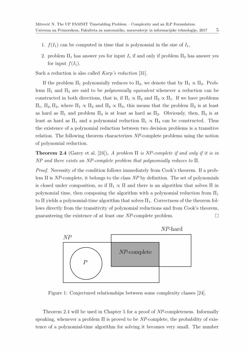
problems proved to be NP-complete. A conjectured relationships between complexity
classes mentioned here is displayed in Figure 1.
One of the fundamental results considering the class of NP-complete problems is
known as Cook’s Theorem [13]. That is the result proving NP-completeness of a
problem called Satisfiability and represents the first NP-completeness proof in the
literature, guaranteeing that the set of NP-complete problems is non-empty. The Sat-
isfiability problem can be defined as follows:
SATISFIABILITY
Instance: A set U of binary variables x1, x2, . . . , xn, a collection C of clauses
representing disjunctions of elements in U or their negations.
Question: Is there a satisfying truth assignment for C?
In order to prove that some problem Π belongs to the class of NP-complete prob-
lems, it suffices to show that Π ∈ NP and that Π is at least as hard as some other
problem in NP, or, in other words, that using a polynomial time algorithm for prob-
lem Π we can construct a polynomial time algorithm for some problem in NP. Such a
correspondence between two problems is called a polynomial reduction.
Definition 2.3. A decision problem Π1 can be polynomially reduced to a decision
problem Π2 if there exists a function f that, given an input I1 for Π1, constructs an
input I2 = f(I1) for Π2 and has the following properties:
Mitrovic N. The UP FAMNIT Timetabling Problem – Complexity and an ILP Formulation.
Univerza na Primorskem, Fakulteta za matematiko, naravoslovje in informacijske tehnologije, 2017 5
1. f(I1) can be computed in time that is polynomial in the size of I1,
2. problem Π1 has answer yes for input I1 if and only if problem Π2 has answer yes
for input f(I1).
Such a reduction is also called Karp’s reduction [31].
If the problem Π1 polynomially reduces to Π2, we denote that by Π1 ∝ Π2. Prob-
lems Π1 and Π2 are said to be polynomially equivalent whenever a reduction can be
constructed in both directions, that is, if Π1 ∝ Π2 and Π2 ∝ Π1. If we have problems
Π1, Π2,Π3, where Π1 ∝ Π2 and Π2 ∝ Π3, this means that the problem Π2 is at least
as hard as Π1 and problem Π3 is at least as hard as Π2. Obviously, then, Π3 is at
least as hard as Π1 and a polynomial reduction Π1 ∝ Π3 can be constructed. Thus
the existence of a polynomial reduction between two decision problems is a transitive
relation. The following theorem characterizes NP-complete problems using the notion
of polynomial reduction.
Theorem 2.4 (Garey et al. [24]). A problem Π is NP-complete if and only if it is in
NP and there exists an NP-complete problem that polynomially reduces to Π.
Proof. Necessity of the condition follows immediately from Cook’s theorem. If a prob-
lem Π is NP-complete, it belongs to the class NP by definition. The set of polynomials
is closed under composition, so if Π1 ∝ Π and there is an algorithm that solves Π in
polynomial time, then composing the algorithm with a polynomial reduction from Π1
to Π yields a polynomial-time algorithm that solves Π1. Correctness of the theorem fol-
lows directly from the transitivity of polynomial reductions and from Cook’s theorem,
guaranteeing the existence of at least one NP-complete problem.
NP
P
NP-hard
NP-complete
Figure 1: Conjectured relationships between some complexity classes [24].
Theorem 2.4 will be used in Chapter 5 for a proof of NP-completeness. Informally
speaking, whenever a problem Π is proved to be NP-complete, the probability of exis-
tence of a polynomial-time algorithm for solving it becomes very small. The number
Mitrovic N. The UP FAMNIT Timetabling Problem – Complexity and an ILP Formulation.
Univerza na Primorskem, Fakulteta za matematiko, naravoslovje in informacijske tehnologije, 2017 6
of steps needed to solve some NP-complete problem using existing algorithms grows
very fast as the size of input increases. Under the assumption that P 6= NP , finding
solutions to large instances of such problems can be very difficult to do in real time.
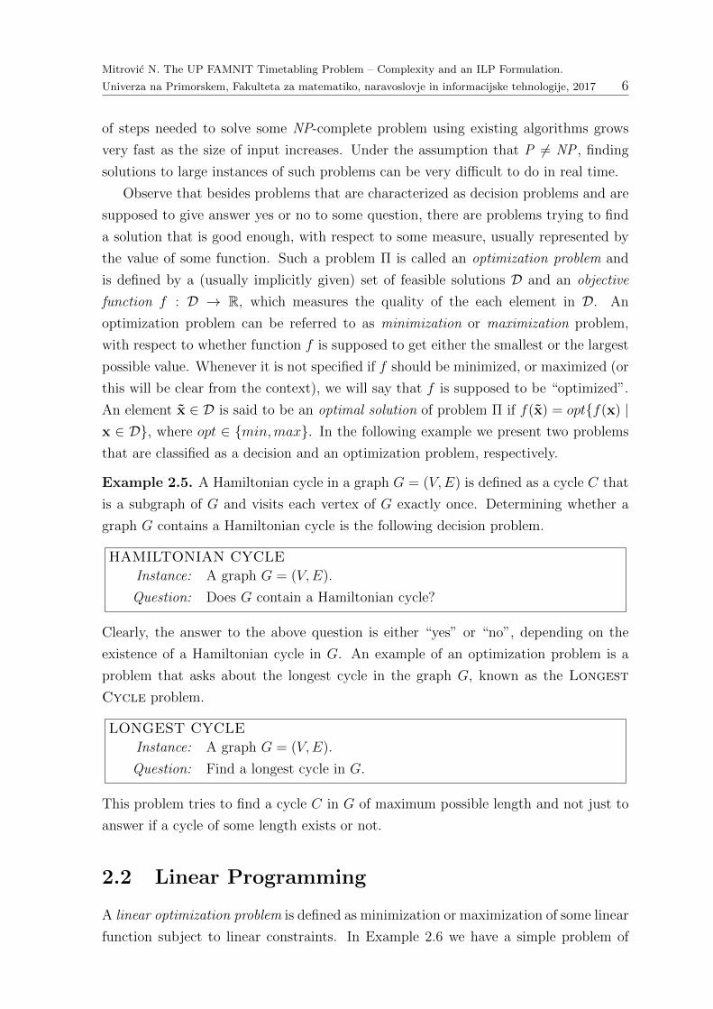
Observe that besides problems that are characterized as decision problems and are
supposed to give answer yes or no to some question, there are problems trying to find
a solution that is good enough, with respect to some measure, usually represented by
the value of some function. Such a problem Π is called an optimization problem and
is defined by a (usually implicitly given) set of feasible solutions D and an objective
function f : D → R, which measures the quality of the each element in D. An
optimization problem can be referred to as minimization or maximization problem,
with respect to whether function f is supposed to get either the smallest or the largest
possible value. Whenever it is not specified if f should be minimized, or maximized (or
this will be clear from the context), we will say that f is supposed to be “optimized”.
An element x ∈ D is said to be an optimal solution of problem Π if f(x) = opt{f(x) |x ∈ D}, where opt ∈ {min,max}. In the following example we present two problems
that are classified as a decision and an optimization problem, respectively.
Example 2.5. A Hamiltonian cycle in a graph G = (V,E) is defined as a cycle C that
is a subgraph of G and visits each vertex of G exactly once. Determining whether a
graph G contains a Hamiltonian cycle is the following decision problem.
HAMILTONIAN CYCLE
Instance: A graph G = (V,E).
Question: Does G contain a Hamiltonian cycle?
Clearly, the answer to the above question is either “yes” or “no”, depending on the
existence of a Hamiltonian cycle in G. An example of an optimization problem is a
problem that asks about the longest cycle in the graph G, known as the Longest
Cycle problem.
LONGEST CYCLE
Instance: A graph G = (V,E).
Question: Find a longest cycle in G.
This problem tries to find a cycle C in G of maximum possible length and not just to
answer if a cycle of some length exists or not.
2.2 Linear Programming
A linear optimization problem is defined as minimization or maximization of some linear
function subject to linear constraints. In Example 2.6 we have a simple problem of
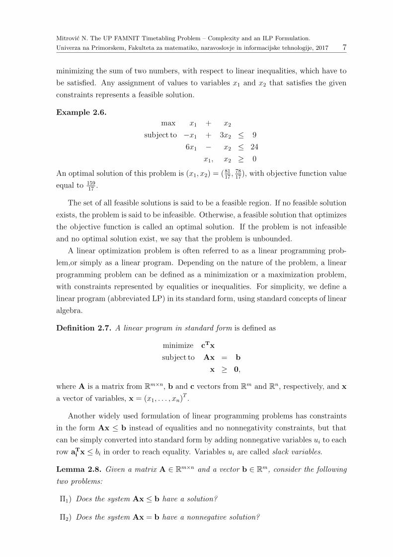
Mitrovic N. The UP FAMNIT Timetabling Problem – Complexity and an ILP Formulation.
Univerza na Primorskem, Fakulteta za matematiko, naravoslovje in informacijske tehnologije, 2017 7
minimizing the sum of two numbers, with respect to linear inequalities, which have to
be satisfied. Any assignment of values to variables x1 and x2 that satisfies the given
constraints represents a feasible solution.
Example 2.6.
max x1 + x2
subject to −x1 + 3x2 ≤ 9
6x1 − x2 ≤ 24
x1, x2 ≥ 0
An optimal solution of this problem is (x1, x2) = (8117, 78
17), with objective function value
equal to 15917
.
The set of all feasible solutions is said to be a feasible region. If no feasible solution
exists, the problem is said to be infeasible. Otherwise, a feasible solution that optimizes
the objective function is called an optimal solution. If the problem is not infeasible
and no optimal solution exist, we say that the problem is unbounded.
A linear optimization problem is often referred to as a linear programming prob-
lem,or simply as a linear program. Depending on the nature of the problem, a linear
programming problem can be defined as a minimization or a maximization problem,
with constraints represented by equalities or inequalities. For simplicity, we define a
linear program (abbreviated LP) in its standard form, using standard concepts of linear
algebra.
Definition 2.7. A linear program in standard form is defined as
minimize cTx
subject to Ax = b
x ≥ 0,
where A is a matrix from Rm×n, b and c vectors from Rm and Rn, respectively, and x
a vector of variables, x = (x1, . . . , xn)T .
Another widely used formulation of linear programming problems has constraints
in the form Ax ≤ b instead of equalities and no nonnegativity constraints, but that
can be simply converted into standard form by adding nonnegative variables ui to each
row aTi x ≤ bi in order to reach equality. Variables ui are called slack variables.
Lemma 2.8. Given a matrix A ∈ Rm×n and a vector b ∈ Rm, consider the following
two problems:
Π1) Does the system Ax ≤ b have a solution?
Π2) Does the system Ax = b have a nonnegative solution?
Mitrovic N. The UP FAMNIT Timetabling Problem – Complexity and an ILP Formulation.
Univerza na Primorskem, Fakulteta za matematiko, naravoslovje in informacijske tehnologije, 2017 8
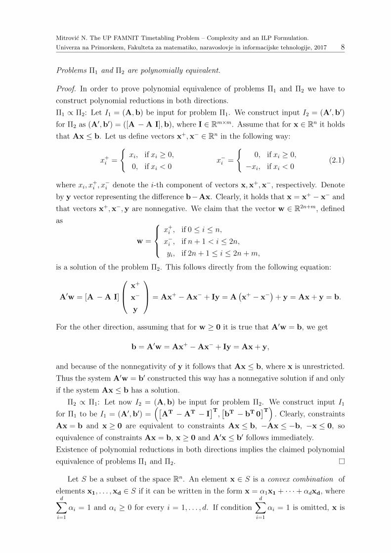
Problems Π1 and Π2 are polynomially equivalent.
Proof. In order to prove polynomial equivalence of problems Π1 and Π2 we have to
construct polynomial reductions in both directions.
Π1 ∝ Π2: Let I1 = (A,b) be input for problem Π1. We construct input I2 = (A′,b′)
for Π2 as (A′,b′) = ([A −A I],b), where I ∈ Rm×m. Assume that for x ∈ Rn it holds
that Ax ≤ b. Let us define vectors x+,x− ∈ Rn in the following way:
x+i =
{xi, if xi ≥ 0,
0, if xi < 0x−i =
{0, if xi ≥ 0,
−xi, if xi < 0(2.1)
where xi, x+i , x
−i denote the i-th component of vectors x,x+,x−, respectively. Denote
by y vector representing the difference b−Ax. Clearly, it holds that x = x+ − x− and
that vectors x+,x−,y are nonnegative. We claim that the vector w ∈ R2n+m, defined
as
w =
x+i , if 0 ≤ i ≤ n,
x−i , if n+ 1 < i ≤ 2n,
yi, if 2n+ 1 ≤ i ≤ 2n+m,
is a solution of the problem Π2. This follows directly from the following equation:
A′w = [A −A I]
x+
x−
y
= Ax+ −Ax− + Iy = A(x+ − x−
)+ y = Ax + y = b.
For the other direction, assuming that for w ≥ 0 it is true that A′w = b, we get
b = A′w = Ax+ −Ax− + Iy = Ax + y,
and because of the nonnegativity of y it follows that Ax ≤ b, where x is unrestricted.
Thus the system A′w = b′ constructed this way has a nonnegative solution if and only
if the system Ax ≤ b has a solution.
Π2 ∝ Π1: Let now I2 = (A,b) be input for problem Π2. We construct input I1
for Π1 to be I1 = (A′,b′) =([
AT −AT − I]T,[bT − bT 0
]T). Clearly, constraints
Ax = b and x ≥ 0 are equivalent to constraints Ax ≤ b, −Ax ≤ −b, −x ≤ 0, so
equivalence of constraints Ax = b, x ≥ 0 and A′x ≤ b′ follows immediately.
Existence of polynomial reductions in both directions implies the claimed polynomial
equivalence of problems Π1 and Π2.
Let S be a subset of the space Rn. An element x ∈ S is a convex combination of
elements x1, . . . ,xd ∈ S if it can be written in the form x = α1x1 + · · ·+ αdxd, whered∑
i=1
αi = 1 and αi ≥ 0 for every i = 1, . . . , d. If conditiond∑
i=1
αi = 1 is omitted, x is

Mitrovic N. The UP FAMNIT Timetabling Problem – Complexity and an ILP Formulation.
Univerza na Primorskem, Fakulteta za matematiko, naravoslovje in informacijske tehnologije, 2017 9
said to be a conical combination of elements x1, . . . ,xd. We say that a set S is convex
if it contains all convex combinations of its elements. Similarly, if a set S contains all
conical combinations of elements in S, then S is called a (convex) cone. A convex hull
of a set S is the smallest convex set containing S, while a cone generated by S is the
smallest cone containing S.
A polyhedron P ⊆ Rn is a set that can be characterised as {x | Ax ≤ b} for some
matrix A ∈ Rm×n and vector b ∈ Rm. A hyperplane and a linear halfspace are sets
defined as {x | aTx = δ} and {x | aTx ≤ δ}, where a is a nonzero vector and δ a scalar.
A point x ∈ P is said to be an extreme point of P if for any two points x1,x2 ∈ P and
scalar λ ∈ (0, 1) equality λx1 + (1− λ)x2 = x implies that x = x1 = x2.
Observe that there is a connection between the definition of a polyhedron and the
feasible region of a linear program. Based on that, a linear program can be represented
graphically, where the optimization of linear function is equivalent to looking for a point
representing the intersection of a hyperplane corresponding to the objective function,
moved in the direction of its normal vector as much as possible, and of a polyhedron
P [52]. During the development of approaches for solving linear programming problems
some important results concerning optimal solutions were derived. One of these results
says that the optimal value of a linear program in standard form, if it exists, is achieved
by some extreme point of P where P is the polyhedron representing the set of feasible
solutions of a linear programm. This statement is proved within the proof of correctness
of simplex algorithm for solving linear programs (see [14]).
In the rest of the thesis, we will denote by I and 0 the identity matrix and the
zero vector of dimensions that will be clear from the context, respectively. In order
to derive results concerning feasibility of a linear program, we introduce the following
theorem.
Theorem 2.9 (see, e.g., Schrijver [51]). Let a1, . . . am,b be vectors in Rn. Then ei-
ther b belongs to the convex cone generated by vectors a1, . . . , am, or there exists a
hyperplane {x | cTx = 0}, such that cTb < 0 and cTai ≥ 0 for i = 1, . . . ,m.
Theorem 2.9 states that, if b is not a nonnegative linear combination of vectors ai,
then there is a hyperplane that separates b from all vectors ai, i = 1, . . . ,m. A proof
of Theorem 2.9, often called the “Fundamental theorem of linear inequalities”, can be
found in Schrijver’s comprehensive monograph [51]. Using Theorem 2.9 we can prove
a basic result concerning feasibility of the linear program, known as Farkas’ lemma.
Theorem 2.10 (Farkas’ lemma [22]). Given a matrix A ∈ Rm×n and a vector b ∈ Rm,
there exists a vector x ∈ Rn that satisfies Ax ≤ b if and only if for each nonnegative
vector y ∈ Rm with ATy = 0 we have bTy ≥ 0.
Mitrovic N. The UP FAMNIT Timetabling Problem – Complexity and an ILP Formulation.
Univerza na Primorskem, Fakulteta za matematiko, naravoslovje in informacijske tehnologije, 2017 10
Proof. (⇒) Suppose that there exists a vector x such that Ax ≤ b. Then, for every
y ≥ 0 such that ATy = 0, we have bT − (Ax)T ≥ 0. Multiplying the last inequality
by nonnegative vector y gives us the desired result bTy ≥ xTATy = xT0 = 0.
(⇐) Let bTy ≥ 0 whenever y is a nonnegative vector such that ATy = 0. Assume for
a contradiction contrary that the system Ax ≤ b does not have a feasible solution.
From the proof of Lemma 2.8 it follows that the system Wx = b, where W = [A−A I]
and x is a vector of variables, has no nonnegative solution. If the columns of W are
denoted by w1, . . .w2n+m, then b cannot be a nonnegative linear combination of them,
thus b is not an element of the cone generated by vectors w1, . . . ,w2m+n (remember
that the first n of them are exactly the columns of matrix A). From Theorem 2.9 it
follows that there is a hyperplane {x | yTx = 0} such that bTy < 0 and yTwi ≥ 0,
i = 1, . . . , 2n + m. A set of inequalities yTwi ≥ 0, i = 1, . . . , 2n + m is equivalent
to the inequality yTW ≥ 0. If we apply the definition of the matrix W, we get the
inequality yT[A −A I] ≥ 0, or equivalently:
yTA ≥ 0, −yTA ≥ 0, yT ≥ 0.
Clearly, it is true that yTA = 0. Since y is a nonnegative vector and bTy ≤ 0, we
have a contradiction, so the statement is proved.
Example 2.11. Suppose we have a following linear program:
min x1 + x2
subject to −x1 + 2x2 ≤ 0
2x1 − x2 ≤ 2
− x2 ≤ −2.
In this LP we have
c =
[1
1
],b =
0
2
−2
,A =
−1 2
2 −1
0 −1
.
If we take y = (2, 1, 3)T , what we get is ATy = 0 and bTy = −4 < 0. From The-
orem 2.10 it follows that the system Ax ≤ b is infeasible. This means that there is
a hyperplane H defined by positive normal vector y that contains vectors defined as
columns of A. Moreover, it holds that vectors y and b belong to distinct half-spaces
with respect to hyperplane H. Since our example is in space of dimension three, the
hyperplane is of dimension two, that is, it is a plane. In Figure 2 we can see the plane H
generated by normal vector y = (2, 1, 3)T and containing vectors a1, a2. As expected,
vectors y and b belong to the distinct halfspaces with respect to the hyperplane H.

Mitrovic N. The UP FAMNIT Timetabling Problem – Complexity and an ILP Formulation.
Univerza na Primorskem, Fakulteta za matematiko, naravoslovje in informacijske tehnologije, 2017 11
y
b
a1
a2
H
Figure 2: A plane through the origin with normal vector y (blue) containing vectors
a1, a2 (black) and separating vector b (red) from vector y.
Some of the most important results concerning linear programming consider pairs
of dual programs, and are known in literature as the Duality Theory of Linear Pro-
gramming.
Definition 2.12. Given a linear program
minimize cTx
subject to Ax ≤ b,(2.2)
its dual linear program is defined as
maximize bTy
subject to ATy = c
y ≥ 0.
(2.3)
The initial linear program is said to be primal.
In particular, for every row aTi of matrix A there is one dual variable yi. All
restrictions on variable yi are derived from the corresponding constraint (see, e.g., [43])
and such dependencies between dual variables and corresponding row constraints are,
for the general case, presented in Table 1.
Constraint in the primal aTi x ≤ bi aT
i x = bi aTi x ≥ bi
Constraint on the dual variable yi ≥ 0 yi unrestricted yi ≤ 0
Table 1: Restrictions of dual variables.
Mitrovic N. The UP FAMNIT Timetabling Problem – Complexity and an ILP Formulation.
Univerza na Primorskem, Fakulteta za matematiko, naravoslovje in informacijske tehnologije, 2017 12
Observe that the dual problem itself is a linear program, so it makes sense to think
about the dual of the dual problem. In the following theorem we characterize the
program obtained by applying two sequential duality operations.
Theorem 2.13. A primal LP problem is polynomially equivalent to the dual of its
dual.
Proof. Suppose we are given a pair of primal and dual LP problems, as in (2.2) and
(2.3), respectively. The dual problem can be equivalently written in the following form:
−min −bTy
subject to ATy ≤ c
−ATy ≤ −c
−y ≤ 0.
The dual of the above problem can be derived using Definition 2.12 and is equal to:
−max[cT − cT 0T
] z1
z2
z3
subject to [A −A − I]
z1
z2
z3
= b
z1, z2, z3 ≥ 0.
(2.4)
The above problem represents the dual of the dual of the primal problem. Note that
with minor changes it can be written in the equivalent form of inequalities with no
nonnegativity constraints:
−max cT (z1 − z2)
subject to A(z1 − z2) − z3 = −b
z1, z2, z3 ≥ 0.
(2.5)
Note that it holds that −max cT (z1 − z2) = min−cT (z1 − z2) = min cT (z2 − z1).
Now we get equivalent form of the problem (2.5):
min cT (z2 − z1)
subject to A (z2 − z1) + z3 = b
z1, z2, z3 ≥ 0.
(2.6)
Setting the x = z2 − z1 and using the proof of Lemma 2.8 we get that the above
problem is equivalent to the initial primal problem, that is min{cTx | Ax ≤ b}.
By Theorem 2.13, the duality operators is in some sense an involution. This explains
its name.

Mitrovic N. The UP FAMNIT Timetabling Problem – Complexity and an ILP Formulation.
Univerza na Primorskem, Fakulteta za matematiko, naravoslovje in informacijske tehnologije, 2017 13
Theorem 2.14 (The LP Duality Theorem). If a linear program has a finite opti-
mal value, then so does its dual and the optimal values are equal. If the problem is
unbounded, then its dual is infeasible.
Proof. Let the primal LP problem be given in standard form, min{cTx | Ax =
b,x ≥ 0}. Its dual is max{bTy | ATy ≤ c}. For every pair of feasible solutions
x,y of the primal and dual problems, respectively, we have
cTx ≥ yTAx = yTb (2.7)
so the optimal value of the dual problem is bounded from above by the optimal value
of the primal problem. We construct a new LP problem consisting of the combined
constraints of the primal and dual problems and requiring additionally that cTx ≤ bTy.
This LP problem is feasible if and only if equality in the inequality (2.7) is reached.
The objective function of the new LP has no influence to the existence of a feasible
solution (it could be a constant), so here we only list the constraints. Vectors x and y
represent vectors of variables. The constraints are:
Ax = b
ATy ≤ c
cTx ≤ bTy
−x ≤ 0.
Putting these constraints into matrix form givesA 0
−A 0
0 AT
−I 0
cT −bT
[
x
y
]≤
b
−b
c
0
0
. (2.8)
From Theorem 2.10 it follows that a pair of vectors x and y satisfying the above
system of inequalities exist if and only if for an arbitrary nonnegative vector z equality
ATz = 0 implies bTz ≥ 0, where Ax ≤ b represents the system (2.8).
Let z =(sT, tT,uT,vT,w
)Tbe a nonnegative vector, where s, t ∈ Rm, u,v ∈ Rn, w ∈
R. Based on the above corollary, we have to prove the following statement: if Au −wb = 0 and ATs−ATt + v + wc = 0, then bTs− bTt + cTu ≥ 0. We consider two
cases.
First, let w > 0. Then
cTu = w−1(wcT
)u = w−1
(vT − sTA + tTA
)u = w−1vTu− w−1(s− t)TAu =
= w−1vTu− w−1(s− t)Twb = w−1vTu− bT (s− t).
Mitrovic N. The UP FAMNIT Timetabling Problem – Complexity and an ILP Formulation.
Univerza na Primorskem, Fakulteta za matematiko, naravoslovje in informacijske tehnologije, 2017 14
Thus, cTu + bT (s− t) = w−1vTu ≥ 0. All equalities follow directly from the assump-
tions.
If w = 0, the assumptions becomes equal to Au = 0 and ATs−ATt−v = 0. Suppose
that x0 and y0 are feasible solutions of the primal and the dual problem, respectively:
Ax0 = b, x0 ≥ 0, ATy0 ≤ c. It follows that cTu ≥ yT0 Au = 0 and, on the other hand,
xT0 AT(s− t) = bT(s− t). These two expressions together give the desired result:
bT(s− t) + cTu = xT0 AT(s− t) + cTu ≥ xT
0 v + yT0 Au = x0v ≥ 0.
If the dual problem is feasible, then the objective function value bTy0 where y0 is an
arbitrary feasible solution (of the dual), gives a lower bound for the optimal value of
the primal. Thus, if the dual is feasible, then the primal cannon be unbounded. This
proves the last statement of the theorem.
In general, Linear Programming is an area with a lot of theoretical results that is
also successfully used in applications. One of the main tools for solving LP problems
is the simplex method, developed by Dantzig in 1947 [14]. Algorithms based on the
simplex method are very efficient from the practical point of view, although the same
does not hold for their theoretical aspects. Recall that if an optimal solution of an LP
in standard form exists, then there is always an extreme point x of the corresponding
polyhedron so that the objective function value at x is optimal. The simplex method is
based on that result. The algorithm runs over vertices of polyhedron P and tries to find
a vertex with minimal objective value. Starting with some vertex, the simplex method
constructs a path of consecutively adjacent vertices of P , until finding an optimal
vertex. The order in which the vertices are visited is crucial for the performance of
simplex method, since it is responsible to prevent cycling in a set of vertices of equal
objective function value, and may enhance the speed of the search.
A step of the simplex algorithm where a way of choosing the next visited vertex is
defined is referred to in the literature as a pivoting step and any method describing the
pivoting steps is called a pivoting rule. The most known pivoting rules are: Dantzig’s
rule (also called the nonbasic gradient method), which was part of the original definition
of simplex method due to Dantzig [14], Bland’s pivoting rule [6], which is the most used
rule in the description of simplex method in literature, the steepest edge rule, defined by
Dickson and Frederick [19], Borgwardts’ pivoting rule [7], etc. A common property of
these rules is that none of them can guarantee to find an optimal solution in polynomial
time in the worst case. It is not known if a pivoting rule for which the simplex method
would work in polynomial time can be constructed, but for known pivoting rules this
is not the case [33]. Feasible regions of known instances of LP problems on which the
simplex method runs exponentially long are deformations of the n-dimensional cube.
However, a simplex method gives good results, since it is proved to find an optimal

Mitrovic N. The UP FAMNIT Timetabling Problem – Complexity and an ILP Formulation.
Univerza na Primorskem, Fakulteta za matematiko, naravoslovje in informacijske tehnologije, 2017 15
solution in polynomial time on average. In particular, for the improved Borgwardt’s
pivoting rule it is proved that the average number of pivot steps is linear in the size of
input data (see, e.g., [51]).
Observe that nonpolynomial running time of the simplex method does not imply
nonpolynomial time complexity of linear programming. In fact, there are other methods
for solving LP problems, which were proved to be polynomial, even if they are not so
efficient in practical use. One of them is the ellipsoid method. The ellipsoid method was
first developed for minimization of convex function and then applied to minimization
of a linear function over a polyhedron. Later it was used by Khachiyan to prove
polynomial-time solvability of LP [32]. The method is based on iterative construction of
n-dimensional ellipsoids, with strictly decreasing volumes in each step of the iteration.
Each ellipsoid contains a polyhedron P that represents a set of feasible solutions of a
problem. Thus, if in the some step of iteration we get the sufficiently small ellipsoid, we
conclude that there corresponding problem is infeasible. If E1 is the initial ellipsoid,
containing polyhedron P , with center in x1, the method checks if x1 is a feasible
solution. If yes, the method stops and outputs the feasible solution x1. Otherwise, the
method removes a set S of points, which do not satisfy some of the constraints defining
P . A new, smaller ellipsoid containing the set E1 \ S is constructed. Clearly, removed
points are not contained in the set P , so P ⊆ E1. If at some step of iteration we get the
ellipsoid containg no points, we can conclude that the set P is empty and the problem
is infeasible. A detailed description of the ellipsoid method is beyond the scope of this
work and can be found e.g., in [51]. The method is polynomial in the worst case and
its running time does not depend on the number of rows of input data (equivalently:
it does not depend on the number of constraints of the LP), just on coefficient values
and number of variables.
Thus, the method is mainly used for finding the feasible solution of the given LP
problem, if one exists. If there is a finite optimal solution, then by The LP Duality
Theorem (Theorem 2.14), there also exists an optimum of a dual program. In that
case the method can be used to find a feasible solution of the LP defined as in equation
(2.8), since it corresponds to an optimal solution of the initial LP problem.
While the ellipsoid method has important theoretical meaning, in practical use it
is not efficient. In higher dimensions it is not numerically stable even for problems of
small size. Unlike the ellipsoid method, the method referred to as the interior point
method, developed by Karmarkar [30], is good at both aspects: in theory it solves LP
problems in polynomial time and it is also efficiently used in practice (see, e.g., [5]).

Mitrovic N. The UP FAMNIT Timetabling Problem – Complexity and an ILP Formulation.
Univerza na Primorskem, Fakulteta za matematiko, naravoslovje in informacijske tehnologije, 2017 16
2.3 Integer Linear Programming
Integer linear programming (abbreviated ILP) is an extension of linear programming
and a useful tool for solving NP-hard combinatorial optimization problems. Indeed,
many such problems ask for either the existence of a subset of a given set satisfying
certain requirements (e.g., a Hamiltonian cycle in a graph) or for a subset that optimizes
a given linear weight function (e.g., a maximum weight independent set in a graph).
This naturally leads to the introduction of binary variables, one for each element of
the ground set, which model the choice of a subset of the set. Additional properties
that every feasible solution should possess are modelled with linear constraints.
ILP can be defined in a few equivalent ways. One of the most commonly used
definitions is the following.
Definition 2.15. An integer linear program is the following optimization problem:
minimize cTx
subject to Ax ≤ b
x ≥ 0
x ∈ Zn,
(2.9)
where A ∈ Rm×n, b ∈ Rm, c ∈ Rn and x is a vector of integer variables, x = (x1, . . . xn).
The parameters A,b, c are usually assumed to have integer components. Note that
equivalent definitions of ILP can be obtained either by putting the equalities instead of
inequalities or by discarding a nonnegativity constraint. The LP relaxation of the above
ILP problem is the LP problem obtained from it by dropping the integrality constraint,
that is, min{cTx | Ax ≤ b,x ≥ 0}. Clearly, the optimal value of the LP relaxation of
given ILP problem is at least as good as the optimal value of the ILP problem. Let Π1
denote the ILP maximization problem, let ΠLP1 denote its LP relaxation and let ΠLP2
be the dual LP of the ΠLP1 . Then, if Π2 denotes the ILP obtained by adding integrality
constraint to all variables of ΠLP2 , using the LP Duality Theorem (Theorem 2.14) we
get:
max(Π1) ≤ max(ΠLP1) = min(ΠLP2) ≤ min(Π2), (2.10)
provided ΠLP1 has a finite optimal value. The inequalities in (2.10) can be strict, that
is, equality of LP relaxed optima for the primal and dual problems does not imply
equality in ILP version. Thus, for integer linear programming problems there is no
duality theorem analogous to Theorem 2.14. ILP seems to be more difficult than LP.
In order to make this statement more precise, let us define the decision version of the
problem.
Mitrovic N. The UP FAMNIT Timetabling Problem – Complexity and an ILP Formulation.
Univerza na Primorskem, Fakulteta za matematiko, naravoslovje in informacijske tehnologije, 2017 17
Integer Linear Programming
Instance: A matrix A ∈ Rm×n, a vector b ∈ Rm.
Question: Does the inequality Ax ≤ b have an integral solution x?
The intuition is confirmed by the following theorem.
Theorem 2.16. Integer Linear Programming is NP-complete.
Integer linear programming represents one of the 21 Karp’s NP-complete
problems [31]. Since it is one of the basic NP-complete problems, few distinct ideas
of proofs of its NP-completeness can be found in the literature. Here we refer the
reader to the most basic one, based on a polynomial reduction from Satisfiability,
which can be found in [51]. In a geometric interpretation, an ILP problem represents
optimizating a given linear function over the set of integer lattice points in a given
polyhedron. Let us define the integer hull P ′ of a polyhedron P to be the smallest
convex set containing the integral vectors of P . Obviously, P ′ ⊆ P and an integer
linear program over P is equivalent to the corresponding linear program over P ′. A
polyhedron for which P = P ′ is called an integral polyhedron. Thus an integer linear
programming problem over an integral polyhedron P is equivalent to its LP relaxation
and so can be solved in polynomial time.
One more result considering a polynomial instance of integer linear programming
problem is known as Lenstra’s theorem (see [37]). In 1983 Lenstra gave an algorithm
that solves integer linear programming problem with fixed number of variables in time
bounded by a polynomial function of the input. It means that integer linear program-
ming problems for which number n of variables does not depend on the input can be
solved in polynomial time. The degree of the polynomial is an exponential function of
the number of variables, that is, of n.
A variant of ILP where only a subset of the set of variables is restricted to have
integer values is called mixed integer linear programming (MILP). The presence of
variables that are supposed to have integer value makes MILP problems NP-complete.
Since the theoretical aspects of MILP and ILP are rather similar, in the following we
focus on ILP. Although ILP problems in general are very difficult to solve, several
methods were developed that can be helpful for solving such problems.
Cutting-plane methods
A cutting plane method is an iterative method based on successive reductions of the
feasible region until an optimal integer solution is found. This method can be used
for convex continuous optimization, as well as for nonlinear optimization problems.
Suppose that we have an ILP minimization problem, with polyhedron P representing
Mitrovic N. The UP FAMNIT Timetabling Problem – Complexity and an ILP Formulation.
Univerza na Primorskem, Fakulteta za matematiko, naravoslovje in informacijske tehnologije, 2017 18
the feasible region of its LP relaxation. A cutting plane method starts by finding an
optimum of the LP relaxation, say x. We assume that x is a vertex of polyhedron P .
The method checks if x is integral and if this is the case, it terminates. If this is not
the case, then there exists some hyperplane H = {x | aTx = δ} that separates x from
all the integer feasible solutions in P . Algebraically, this means that the inequality
aTx ≤ δ is satisfied by all the integral vectors in P , but not by the vector x.
A hyperplane H as above is called a cut, and is added to the list of hyperplanes
defining P , so that in the next iteration the feasible region is reduced with respect to
the new hyperplane. A cut actually represents an inequality that becomes one more
constraint of the initial ILP problem, called a cut constraint. The process of finding
such an inequality is called the separation problem. The choice of a new constraint can
have a big influence on the result computed by the method and on the time it takes to
solve the initial ILP problem.
Observe that no integer feasible solution is removed from the feasible region during
the execution of the method. The first method with a solution to the separation
problem was the Gomory cutting plane method [26]. The method starts with an ILP
problem, and solves its LP relaxation using the simplex method. If the solution is
not integral, the method uses one of the parameters, which are the result of the simlex
method (a row in the simplex tableau, see e.g., [43]). A new constraint defined that way
is satisfied by all integer feasible solutions, and is violated by the computed optimal
solution of the LP relaxation.
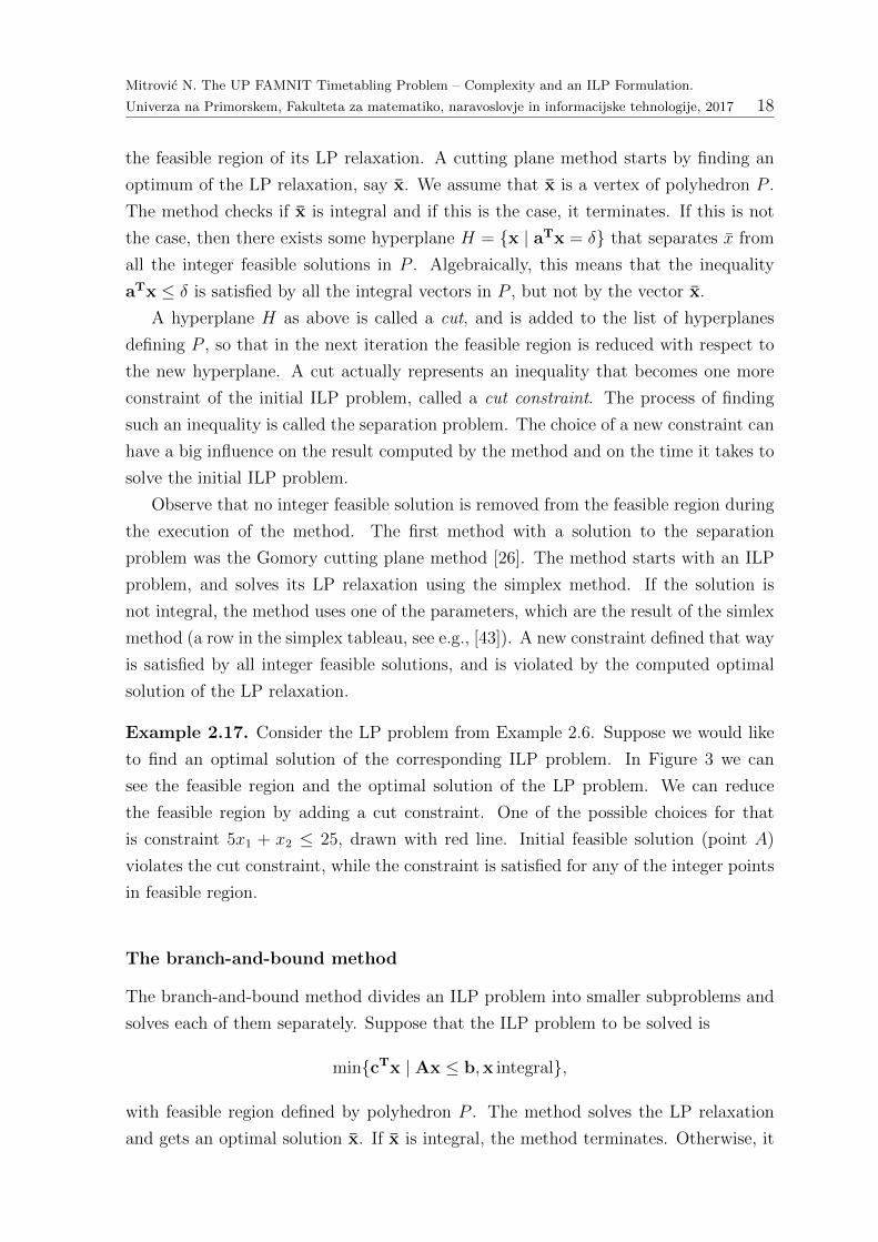
Example 2.17. Consider the LP problem from Example 2.6. Suppose we would like
to find an optimal solution of the corresponding ILP problem. In Figure 3 we can
see the feasible region and the optimal solution of the LP problem. We can reduce
the feasible region by adding a cut constraint. One of the possible choices for that
is constraint 5x1 + x2 ≤ 25, drawn with red line. Initial feasible solution (point A)
violates the cut constraint, while the constraint is satisfied for any of the integer points
in feasible region.
The branch-and-bound method
The branch-and-bound method divides an ILP problem into smaller subproblems and
solves each of them separately. Suppose that the ILP problem to be solved is
min{cTx | Ax ≤ b,x integral},
with feasible region defined by polyhedron P . The method solves the LP relaxation
and gets an optimal solution x. If x is integral, the method terminates. Otherwise, it
Mitrovic N. The UP FAMNIT Timetabling Problem – Complexity and an ILP Formulation.
Univerza na Primorskem, Fakulteta za matematiko, naravoslovje in informacijske tehnologije, 2017 19
2 4 6 8 10
2
4
6
8
10
x1
x2
5x1
+x
2=
25
A
Figure 3: Feasible region, optimal solution of LP relaxed version of problem (point A)
and a cut constraint (blue line) of Example 2.17.
takes a nonintegral component of x, say xi, and separates the initial problem into two
subproblems:
• Π1 : min {cTx | Ax ≤ b, xi ≤ bδc},
• Π2 : min {cTx | Ax ≤ b, xi ≥ dδe},
where δ is the value of component xi. Observe that the feasible regions of these two
problems are disjoint and that all integral vectors from P are contained in their union.
The method constructs a tree, with root of the tree corresponding to the initial problem
and branches corresponding to the problems based on new, separated polyhedra. The
leaves of the tree are either infeasible problems or problems having optimal integral
solutions. The best one among optimal solutions on all the leaves is an optimal solution
of the initial ILP problem.
In this method the main step is breaking a problem into subproblems, that is,
defining which variable the method will branch upon. Once the tree of subproblems
is constructed, it should be searched for an optimal solution. If some node, say A,
gives us an integral optimal value better than the optimal value of some other node,
say B (optimal solution at B is not necessarily integral), we cut the node B, as well
as its branches, since in the subtree corresponding to the node B for sure an opti-
mal solution cannot be found. The objective function value of subproblems increases
(resp. decreases) for minimization (resp. maximization) problems, with every step going
deeper within the tree.
Mitrovic N. The UP FAMNIT Timetabling Problem – Complexity and an ILP Formulation.
Univerza na Primorskem, Fakulteta za matematiko, naravoslovje in informacijske tehnologije, 2017 20
−x1 + 3x2 ≤ 96x1 − x2 ≤ 24
−x1 + 3x2 ≤ 96x1 − x2 ≤ 24x1 ≤ 4
−x1 + 3x2 ≤ 96x1 − x2 ≤ 24x1 ≥ 5
−x1 + 3x2 ≤ 96x1 − x2 ≤ 24x1 ≤ 4
x2 ≤ 4
−x1 + 3x2 ≤ 96x1 − x2 ≤ 24x1 ≤ 4
x2 ≥ 5
OPT = 15917
(x1, x2) =(8117, 7817
)OPT = 25
3
(x1, x2) =(4, 13
3
)INFEASIBLE
INFEASIBLEOPT = 8(x1, x2) = (4, 4)
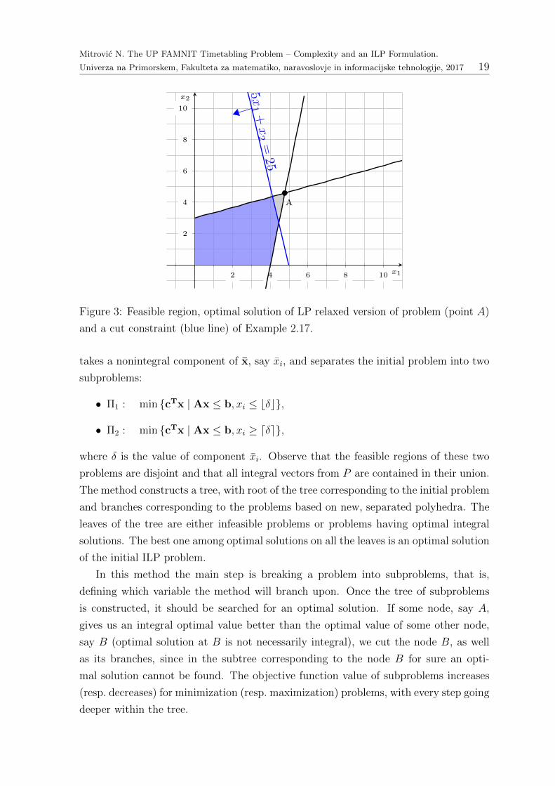
Figure 4: A tree representing branch-and-bound nodes.
Example 2.18. Consider again the problem from Example 2.6. We use the branch-
and-bound method in order to find its optimal integer solution. The unique optimal
solution of the relaxed problem is (x1, x2) = (8117, 78
17), with objective function value 159
17.
Since both variables are non integer, we can choose any one of them for the branching
step. We choose x1. Then we get two new LP problems, similar to the initial ones,
with added constraints x1 ≤ 4 and x1 ≥ 5, respectively. An optimal solution of the
first one is (x1, x2) = (4, 133
) with objective function value 253
, while the LP on the other
branch is infeasible. We continue with branching on variable x2, since it is non-integral.
The added constraints are x2 ≤ 4 and x2 ≥ 5, respectively. Finally, we get an optimal
solution that is integral, (x1, x2) = (4, 4), with objective function value equal to 8. The
corresponding tree is displayed on Figure 4.
Note that the example displayed on Figure 4 is not large enough to show the “bound”
part of the branch-and-bound method. For details regarding the branch-and-bound
method we refer a reader to the paper due to Lawler and Wood, from 1966 [35].
Lagrangean relaxation
Lagrangean relaxation is a method used for determining an upper bound for a max-
imization ILP problem (or a lower bound for a minimization ILP problem), by sep-
arating the set of constraints into two disjoint sets. Let the ILP problem be given
as
min {cTx | Ax ≤ 0,x integer}
and let the set of constraints Ax ≤ b separate into two disjoint sets A1x ≤ b1 and
A2x ≤ b2. Assume that the above problem can be efficiently solved with respect to
Mitrovic N. The UP FAMNIT Timetabling Problem – Complexity and an ILP Formulation.
Univerza na Primorskem, Fakulteta za matematiko, naravoslovje in informacijske tehnologije, 2017 21
constraint A1x ≤ b1, while adding constraint A2x ≤ b2 raises the complexity of the
problem. In that case we include the problematic set of constraints into the objective
function, so that for violation of any constraint δi we add some nonnegative penalty
coefficient αi. If constraint aix ≤ bi is violated, then obviously aix− bi > 0. Consider
the following ILP problem:
minimize cTx + αT (A2x− b2)
subject to A1x ≤ b1
x integer
, (2.11)
where α is a positive vector. The above ILP problem is called the Lagrangean relaxation
of the initial problem. It has a greater set of feasible solutions and gives a lower bound
on the optimal value of the initial problem (see, e.g., [5]).
Theorem 2.19. The optimal value of the Lagrangean relaxation is a lower bound for
the optimal value of the initial ILP problem.
Proof. Let x be an optimal solution of the Lagrangean relaxation problem, and let x
be an optimal solution of the initial problem. Since x is a feasible solution of the ILP
problem, we have A2x− b2 ≤ 0. Then
cTx ≥ cTx + α (A2x− b2) ≥ cTx + αT (A2x− b2) (2.12)
The first inequality holds since α > 0 and A2x − b2 ≤ 0 and the second one is a
consequence of optimality of x in the Lagrangean relaxation problem.
If parameters αi are defined as dual variables (recall from Section 2.2 that every row
of matrix A has a corresponding dual variable), then Theorem 2.19 is referred to as the
Integer Programming Duality Theorem. The problem of minimizing the gap between
these two optimal solutions is called the Lagrangean dual problem [25]. This approach
is very useful for problems with nice structure and efficiently computable feasible set
D = {x integral,A1x ≤ b}.
Dynamic programming
Dynamic programming is a method that breaks a problem into a number of smaller
subproblems and solves them sequentially. Optimal solutions calculated for subprob-
lems are combined in order to get a solution for a larger problem. The method does not
repeat the same calculations, but uses the previously computed solutions. A dynamic
programming approach is used for construction of many efficient algorithms for various
problems (such as the shortest path problem in acyclic digraphs [54], the maximum
weight independent set problem in interval graphs [28], etc.). In integer programming
Mitrovic N. The UP FAMNIT Timetabling Problem – Complexity and an ILP Formulation.
Univerza na Primorskem, Fakulteta za matematiko, naravoslovje in informacijske tehnologije, 2017 22
problems dynamic programming is used mostly in the following way: instead of assign-
ing values to all variables xi at once, we pick up one variable at a time to be assigned
some value. In each step we compute the value of the objective function with respect to
an already known assignment from the previous steps. If we try to assign few distinct
values to variable xi, we choose one that optimizes the objective value. This approach
cannot be simply used in case of general integer variables, it is more appropriate for
binary variables, where there are just two possible assignments for each variable. Using
dynamic programming for binary ILP problems, the complexity of the problems can
be much improved, although it is still exponential, in the size of the coefficients of the
problem [5].
2.3.1 Modelling with ILP
Let Π be a combinatorial optimization problem, that we would like to model using
concepts of integer linear programming. To construct a well-defined model, we have
to determine the set of variables and their domains, the constraints, and the objective
function. For problems where variables model decisions about whether certain events
happen or not, binary variables are often used. These have value 1 if the corresponding
event happens, and 0 otherwise. In this thesis we model the timetabling problem, which
consists of a set of events, so in the following we consider binary variables. The objective
function is a linear function of the defined variables. The main part of ILP problems
are constraints, or, more precisely, the polyhedron defining the feasible region. Let
x1, . . . , xn be a set of binary variables and I some index set. Here we list some basic
ideas, which are used for modelling our timetabling problem:
(I) At most δ events from set I happen:∑i∈I
xi ≤ δ.
(II) At least δ events from set I happen:∑i∈I
xi ≥ δ.
(III) Exactly δ events from set I happen:∑i∈I
xi = δ.
(IV) In optimization problems, it often happens that some requirement consists of
two constraints, which must not be violated at the same time, i.e., at least one
of them should be satisfied. Let requirement P be represented by constraints
aTx ≤ b and cTx ≤ d, where at least one of them should be satisfied. In order
to satisfy requirement P , we introduce a binary variable zP , which is intended to
have value 1 if the first equation of requirement P is satisfied, and 0 if the other
one is satisfied. This will ensure that at least one of the constraints is satisfied.
Mitrovic N. The UP FAMNIT Timetabling Problem – Complexity and an ILP Formulation.
Univerza na Primorskem, Fakulteta za matematiko, naravoslovje in informacijske tehnologije, 2017 23
We add the following constraints to initial problem:
aTx ≤ b+B1 · (1− zP ) ,
cTx ≤ d+B2 · zP ,(2.13)
where B1, B2 are properly selected constants. Observe that it can happen that
both of inequalities are satisfied.
(V) Disjoint constraints can also be successfully modelled using concepts of ILP. Let
requirement C consists of two constraints, which should not be satisfied at the
same time, i.e. at least one of them should be violated. Suppose constraints are
the same as above:
aTx ≤ b and cTx ≤ d. (2.14)
Their complements are constraints aTx > b and cTx > d, which in case of integer
input data and integral variables are equivalent to constraints aTx ≥ b + 1
and cTx ≥ d + 1, respectively. Then the requirement that at least one of
constraints (2.14) is violated is equivalent to requirement that at least one of their
complements is satisfied. We can model it using the point (IV) on complement
constraints.
Mitrovic N. The UP FAMNIT Timetabling Problem – Complexity and an ILP Formulation.
Univerza na Primorskem, Fakulteta za matematiko, naravoslovje in informacijske tehnologije, 2017 24
3 Timetabling problems
In this chapter we introduce the timetabling problem in its general form, basic results
about its computational complexity, as well as a literature overview, with description
of the most common approaches used in modelling timetabling problems.
3.1 The Timetable Design Problem
One of the problems that can be modelled using methods of integer linear programming
is the timetabling problem. The timetabling problem consists in assigning resources
to a set of timeslots. It appears in many fields of everyday life, so depending of the
application, resources could be workers and jobs, students and lectures, sports matches,
etc. Since there are various definitions of timetabling problems, we introduce here one
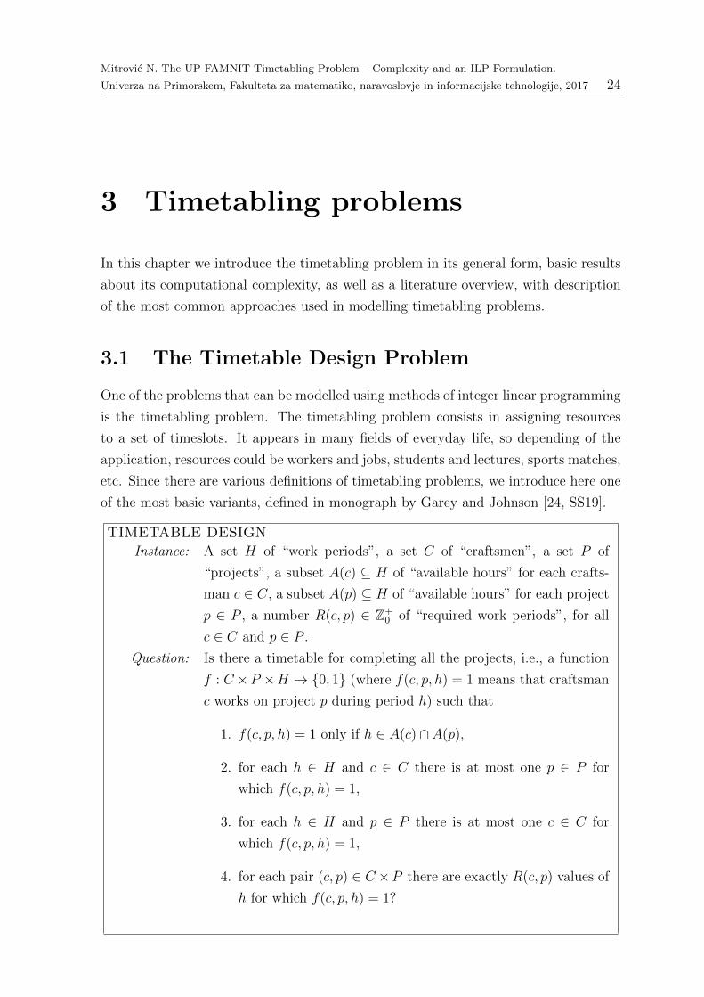
of the most basic variants, defined in monograph by Garey and Johnson [24, SS19].
TIMETABLE DESIGN
Instance: A set H of “work periods”, a set C of “craftsmen”, a set P of
“projects”, a subset A(c) ⊆ H of “available hours” for each crafts-
man c ∈ C, a subset A(p) ⊆ H of “available hours” for each project
p ∈ P , a number R(c, p) ∈ Z+0 of “required work periods”, for all
c ∈ C and p ∈ P .
Question: Is there a timetable for completing all the projects, i.e., a function
f : C ×P ×H → {0, 1} (where f(c, p, h) = 1 means that craftsman
c works on project p during period h) such that
1. f(c, p, h) = 1 only if h ∈ A(c) ∩ A(p),
2. for each h ∈ H and c ∈ C there is at most one p ∈ P for
which f(c, p, h) = 1,
3. for each h ∈ H and p ∈ P there is at most one c ∈ C for
which f(c, p, h) = 1,
4. for each pair (c, p) ∈ C ×P there are exactly R(c, p) values of
h for which f(c, p, h) = 1?
Mitrovic N. The UP FAMNIT Timetabling Problem – Complexity and an ILP Formulation.
Univerza na Primorskem, Fakulteta za matematiko, naravoslovje in informacijske tehnologije, 2017 25
This problem is known to be NP-complete. A proof, based on a polynomial reduction
from Satisfiability, can be found in the paper by Even et al. [21]. The problem
remains NP-complete even if R(c, p) ∈ {0, 1} for all c ∈ C and p ∈ P [24]. The
Timetable Design problem with this restriction will be referred to as the Binary
Timetable Design (BTD) problem.
A feasible solution of this problem is a timetable for completing all projects, or
more precisely, a function f : C × P ×H → {0, 1} that satisfies all listed conditions.
The problem can have additional constraints, which are desired to be satisfied, but
do not necessarily have to hold. For that reason, constraints are divided into two
groups: hard constraints and soft constraints. Hard constraints must be satisfied by a
feasible timetable, while soft constraints represent requirements that are desirable to
be satisfied, but their violation has no influence to the feasibility of the solution. Every
soft constraint has a weight, and in case that the constraint is violated, the weight is
added to the objective function. Therefore, an optimal solution has minimal value of
the objective function and implicitly satisfies as many soft constraints as possible. For
example, in the problem defined above, an additional constraint prohibiting assigning
of craftsman ci at timeslot tj is a hard constraint, while preference of craftsman ci
to project pj over project pk is soft constraint desired to be satisfied, although not
necessarily.
When speaking about a university timetabling problem, resources are defined as
courses, students groups, and sometimes also rooms. The widely used definition for
university course timetabling problem (UCT problem) defines it as scheduling a se-
quence of teaching sessions involving lecturers and students in a predetermined period
of time, normally within a week, while satisfying a set of constraints [49]. Every institu-
tion has its own set of contraints that should be satisfied when constructing a timetable,
so for that reason a general solution for university timetabling problems does not exist.
Some institutions have all lectures of the same length, or timeslots of fixed duration
where any course can be assigned to an arbitrary timeslot. Also, there are institutions
that have a predetermined assignment of rooms to student groups. Many institutions
have elective courses, as well as courses that are common to more than one student
group, while for some institutions this is not the case. For some institutions collisions
between elective subjects for students of same student group are forbidden, while for
some others this is just desirable but not absolutely necessary. These constraints are
generally the main reason for big complexity of timetabling problems [9]. Relaxing
some of them simplifies a timetabling problem and implicitly generates a problem with
smaller complexity. The influence of individual constraints to the complexity of the
whole problem is researched in the literature, so few special types of constraints were
identified as crucial for increased complexity of a timetabling problem.
Mitrovic N. The UP FAMNIT Timetabling Problem – Complexity and an ILP Formulation.
Univerza na Primorskem, Fakulteta za matematiko, naravoslovje in informacijske tehnologije, 2017 26
On the computational complexity of problem variants
Various definitions of a university timetabling problem lead to variations in its compu-
tational complexity. A problem with fewer restrictions and with a small set of resources
to be assigned appears simple in comparison with a more involved problem. However, it
is not easy to define an exact boundary that would determine when a problem becomes
difficult to solve.
In the literature there are studies that consider the problem with some set of con-
straints and then the same problem with the removal of some constraint. The analysis
of the computational complexity of the corresponding problem can thus reveal whether
a removed constraint has any influence on the hardness of the problem. One such anal-
ysis can be found in [39], where the author defined two versions of the problem and
resolved their complexity status. It turned out that timetabling problems concerning
just timeslots and courses, involving lecturers, students, and arbitrarily many arbitrar-
ily large classrooms can be solved in polynomial time. A polynomial-time algorithm
can be obtained using known algorithms for the maximum flow problem, for example
particular the algorithm given due to Ford and Fulkerson [23] with implementation of
Edmonds and Karp [20]. This theoretical result does not seem to have big implica-
tion for real-life timetabling problems, since almost all university timetabling problems
considered in the literature are supposed to also assign courses to classrooms.
The variant of the problem not containing room assignment is similar to highschool
timetabling problems, since each element of the resource set (student group, course,
or lecturer) is supposed to have its own classroom. Another restriction of timetabling
problem that increases the problem complexity, although it is not proved that its
removal makes the problem solvable in polynomial time, is related to length of the
lectures. There are examples of problems concerning lectures of the same length for
which the number of steps needed for solving the problem is significantly reduced in
comparison with the same problems having the lectures of distinct length [15]. Also,
there are algorithms for solving the university timetabling problems that work in two
phases. In the first one constraints requiring consecutive hours of some course are
violated and are recovered during the second one. However, even if the length of the
lectures is the same for all courses, such a problem is still NP-complete [39].
3.2 Literature review
Timetabling problems can be formulated in many different ways, depending on pref-
erences of the institution. Therefore, various models are developed in the literature.
Some constraints are common to many institutions, while some constraints are very
Mitrovic N. The UP FAMNIT Timetabling Problem – Complexity and an ILP Formulation.
Univerza na Primorskem, Fakulteta za matematiko, naravoslovje in informacijske tehnologije, 2017 27
specific. Regarding these specific constraints, authors often try to find some good
enough approach and construct either a new model or further develop the existing one,
in order to solve their own problem. Various approaches were used, including concepts
from graph theory, or more precisely graph colouring, integer linear programming,
metaheuristics, constraint programming, and neural networks.
Graph colouring
Given finite, simple, undirected graph G = (V,E), a proper k-colouring of G is defined
as a function f : V → {1, 2, . . . , k}, such that for adjacent vertices u and v we have
f(u) 6= f(v). A correspondence between graph colourings and timetabling problems
can be understood as follows: we construct a graph G where every vertex represents
one of the events to be scheduled. If two events are in conflict, then in G there is an
edge between corresponding vertices. Thus, every colour in a proper k-colouring of G
represents some time interval and the event corresponding to vertex v can be scheduled
at time corresponding to colour f(v).
One of the first models for university timetabling problem based on graph theory
was presented by Welsh and Powell in 1960s [55]. Graph colouring is a well known NP-
hard problem and several heuristics for the problem are known (see, e.g., [8, 18, 29]).
So if the graph G corresponding to a timetabling problem is sufficiently structured,
some of heuristics can be used. There are also approaches that combine few distinct
heuristics for graph colouring, in such a way that some new heuristic decides which
of the heuristics will be used to colour the vertices of a graph. A description of such
a method used for a timetabling problem is given by Burke et al. [11]. Recent graph
colouring approaches also include assignment of classrooms in the model, so this can
be understood as an advantage of this approach [47]. A disadvantage of the graph
colouring approach is the difficulty of modelling lectures that do not all have the same
length. With one vertex we cannot specify the duration of a lecture in a simple way, so
for institutions where timeslots do not have predefined distinct lengths, it is difficult
to model and evaluate timetabling problems using graph colourings.
Integer linear programming
In Section 2.3 we have seen principles of using integer linear programming for mod-
elling a combinatorial optimization problem. As mentioned there, if the problem to be
solved consists of some events, binary variables can be used. One of the first ideas for
modelling a timetabling problem using integer linear programming was developed for
a school timetable during the 1960s by Lawrie [36]. After that the number of papers
presenting similar models grew rapidly. Models constructed in that time were too big
Mitrovic N. The UP FAMNIT Timetabling Problem – Complexity and an ILP Formulation.
Univerza na Primorskem, Fakulteta za matematiko, naravoslovje in informacijske tehnologije, 2017 28
to be solved in real time, since software developed for that purpose was not fast enough.
The corresponding theoretically developed models were not useful in real-life applica-
tions, which is the main reason for stagnation of this approach during subsequent years.
Nowadays, powerful software is available for solving integer linear programs, so ILP
is again one of the main approaches for solving combinatorial optimization problems,
as well as timetabling problems. There are various models in literature, depending
on constraints and preferences of corresponding institutions. One of them is available
in papers by Daskalaki et al. [16], and by Daskalaki and Birbas [15]), where a huge
set of constraints is represented using linear inequalities. A nice summary of types of
constraints used in the literature is given by Aizam and Caccetta (see [3]), while a good
description of elements of objective function is available in a paper by Pereira and Costa
(see [44]).
Since assignment of courses and rooms for timetabling problems is mostly done
for a period of one week, minor changes in input data for some week may affect the
whole timetable. A problem of finding an assignment x of a set of resources to the
set of variables, such that differences between x and an existing initial assignment are
minimized does not seem to be easily solvable using integer linear programming. One
of the difficulties when using this approach is a big number of variables and constraints
for larger instances of problem. Also, it is often not trivial to model some very specific
constraint, which is not part of requirements at other institutions, and sometimes at
all to understand the timetable from the obtained solution, which is typically a big-
dimensional vector consisting of 0s and 1s.
Metaheuristics
Algorithms that find a solution not relying on any randomness are said to be determin-
istic, while algorithms that contain some random parameters are said to be stochastic.
A topic of main interest in the stochastic approach are metaheuristic algorithms. Con-
cretely, for timetabling problems the most used metaheuristics are genetic algorithms
and local search methods such as simulated annealing and tabu search, which we briefly
describe here (see, e.g., [4, 38]).
Genetic algorithms are based on evolution of some population, which in case of
optimization problems represents the set of feasible solutions of the problem. In order to
apply a genetic algorithm to some problem, several parameters have to be determined:
the crossover operation, the mutation operation, the threshold for elimination, and the
fitness function. Suppose that the initial population consists of distinct timetables,
where each timetable is one individual, consisting of chromosomes. A gene is defined
as a part of chromosome and can be represented using real numbers, binary values, or
alphanumeric characters. In the literature, genes are mostly identified with timeslots
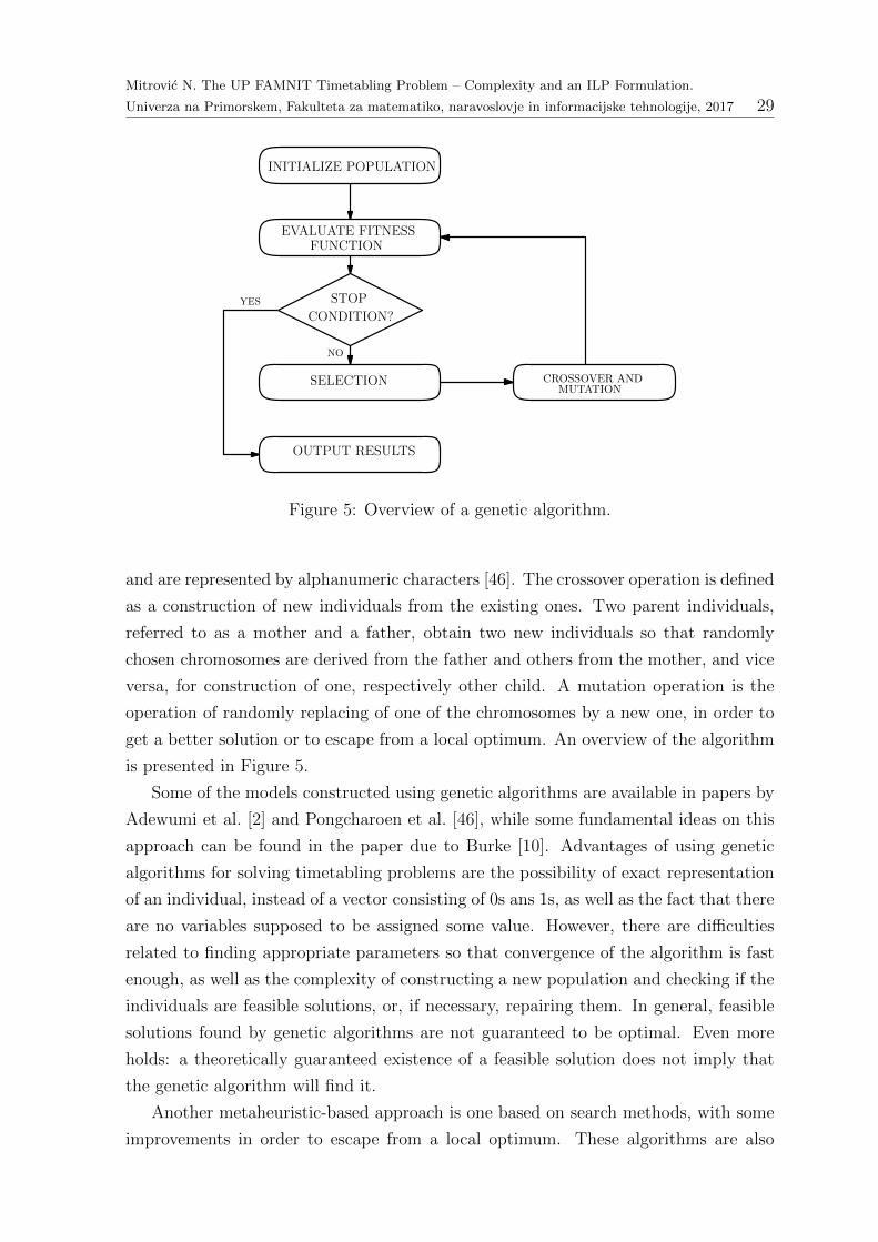
Mitrovic N. The UP FAMNIT Timetabling Problem – Complexity and an ILP Formulation.
Univerza na Primorskem, Fakulteta za matematiko, naravoslovje in informacijske tehnologije, 2017 29
CROSSOVER ANDMUTATION
INITIALIZE POPULATION
EVALUATE FITNESSFUNCTION
STOP
CONDITION?YES
NO
SELECTION
OUTPUT RESULTS
Figure 5: Overview of a genetic algorithm.
and are represented by alphanumeric characters [46]. The crossover operation is defined
as a construction of new individuals from the existing ones. Two parent individuals,
referred to as a mother and a father, obtain two new individuals so that randomly
chosen chromosomes are derived from the father and others from the mother, and vice
versa, for construction of one, respectively other child. A mutation operation is the
operation of randomly replacing of one of the chromosomes by a new one, in order to
get a better solution or to escape from a local optimum. An overview of the algorithm
is presented in Figure 5.
Some of the models constructed using genetic algorithms are available in papers by
Adewumi et al. [2] and Pongcharoen et al. [46], while some fundamental ideas on this
approach can be found in the paper due to Burke [10]. Advantages of using genetic
algorithms for solving timetabling problems are the possibility of exact representation
of an individual, instead of a vector consisting of 0s ans 1s, as well as the fact that there
are no variables supposed to be assigned some value. However, there are difficulties
related to finding appropriate parameters so that convergence of the algorithm is fast
enough, as well as the complexity of constructing a new population and checking if the
individuals are feasible solutions, or, if necessary, repairing them. In general, feasible
solutions found by genetic algorithms are not guaranteed to be optimal. Even more
holds: a theoretically guaranteed existence of a feasible solution does not imply that
the genetic algorithm will find it.
Another metaheuristic-based approach is one based on search methods, with some
improvements in order to escape from a local optimum. These algorithms are also
Mitrovic N. The UP FAMNIT Timetabling Problem – Complexity and an ILP Formulation.
Univerza na Primorskem, Fakulteta za matematiko, naravoslovje in informacijske tehnologije, 2017 30
based on parameters that have a big influence on the result. The two main parameters
are neighbourhood and fitness functions. Given some initial feasible timetable s∗, a
search method evaluate the fitness function on the neighbourhood of s∗ and chooses the
next iteration step with some probability dependent on the value of evaluated function.
These methods require a lot of testing of parameters for their enhancement, especially
for problems where the space of feasible solutions is only a small part of the set of all
solutions (equivalently: of the set of all possible combinations of chromosomes).
Constraint programming
Models based on constraint programming methods contain variables defining events
to be assigned, domains for each variable, and constraints representing relations be-
tween variables that should be satisfied. Contraints can be understood as properties
of variables and this possibility of declarative description of constraints is the biggest
advantage of this approach. However, it can happen that the set of feasible1 solutions
is too small, of even empty, and in that case constraint programming in its usual defi-
nition is not the best method for modelling a problem. Since constraint programming
approach contains variables that are assigned stepwise, a solution where none of the
variables has assigned a value will be referred to as empty solution. Thus, methods for
solving a timetabling problem based on a costraint programming approach start with
an empty solution and assign variables in some order.
A solution is said to be complete if a value is assigned to each variable, and in-
complete otherwise [48]. Such a method is equivalent to searching over a tree where
each node assigns a value to one variable. If it happens that some variable cannot be
assigned a valid value, the algorithm backtracks and checks the other subtree of the
nearest root. A major advantage of this approach is the possibility of solving the min-
imal perturbation problem, i.e., of finding a timetable that contains minimal changes
in comparison with the previous timetable [40]. Observe that in case of an infeasible
problem, the algorithms typically output a solution that has the greatest number of
variables assigned, and the values of other variables can be determined manually. In
that case a person that do it manually decides if some of the hard constraints can be
changed or violated, in order to construct a timetable that is good enough. Methods
based on this approach available in the literature (see, e.g., [41]) are mostly made in
combination with some heuristics or some local search method, e.g., for ordering a
variables (see, e.g., [1]).
Mitrovic N. The UP FAMNIT Timetabling Problem – Complexity and an ILP Formulation.
Univerza na Primorskem, Fakulteta za matematiko, naravoslovje in informacijske tehnologije, 2017 31
Neural networks
Neural networks represent a computational model used for recognizing relations and
patterns in some datasets, based on rules developed on the structure of few elements in
a set. This approach is based on the biological structure of the brain, so it consists of
units called neurons and connections between them, called synapses. Every synapse has
some weight, called capacity, and every connection between the elements of a dataset
can be represented as a weighted connection between two neurons. Development of
neural networks began with a construction of a neural network algorithm that solves
the Travelling Salesman Problem, by Hopfield and Tank in 1985 [27]. Since the results
obtained by Hopfield and Tank were very sensitive to the values of parameters, many
researches believed that optimal selection of these parameters cannot be simply done
and that methods based on neural networks cannot bring good results for combina-
torial optimization problems [53]. Thus, during the years, neural networks have not
been competitive with other approaches when applied to combinatorial optimization
problems [53]. Almost one decade after the paper due to Hopfield and Tank was pub-
lished, concepts of neural networks were successfully applied to a linear programming
problems and that was a breaking point in the development of the neural networks [12].
Nowadays, neural networks are a widely used method for solving combinatorial
optimization problems. In case of the timetabling problem, algorithms are based on
the so-called Hopfield network. As described in the original paper, a Hopfield network
consists of a fully interconnected system of n computational elements or neurons [27].
Defining the possible states of neurons and the activation function as a measure that
decides the active state of a neuron, this method can be efficiently used in modelling
the timetabling problem. An approach based on the Hopfield network is developed by
Smith et al. [53] and represents a model for school timetabling problem. Constraints
of the model are not modelled as special hard requirements, but are included in the
objective function with penalties for each violation. In that case, the objective func-
tion corresponds to the parameter of the neural network, called the energy function. A
disadvantage of this approach is the number of synapses, since addition of one single
neuron to the network increases the number of synapses and implicitly also the com-
plexity of solving the problem. For that reason, algorithms based on neural networks
are often developed in combination with some heuristic methods. This can give very
efficient results [53].
Mitrovic N. The UP FAMNIT Timetabling Problem – Complexity and an ILP Formulation.
Univerza na Primorskem, Fakulteta za matematiko, naravoslovje in informacijske tehnologije, 2017 32
4 The UP FAMNIT timetabling
problem
As already mentioned in previous chapters, there is no general solution for the uni-
versity course timetabling problem, since every institution has its own requirements
and preferences. Thus, in order to model a timetabling problem for some concrete
institution, we have to describe rules and requirements of the institution, which are
relevant for the timetable. In this chapter we first describe informally and then define
formally the timetabling problem for a concrete case of the Faculty of Mathematics,
Natural Sciences and Information Technologies, University of Primorska (abbreviated
UP FAMNIT). Using the description and the definition from this chapter, in Chap-
ter 6 we introduce an integer linear program modelling the corresponding timetabling
problem.
4.1 Description of the teaching process at the in-
stitution
The core of a university timetabling problem is assigning events represented by courses
to ordered pairs of a time interval and a classroom. In this work we construct a
timetable for one week, or more precisely for five working days. Every day consists of
a fixed number of small time intervals, called timeslots.
Each course offered by the faculty has a specified type: lectures, tutorials, or a
combination of both. If a course is a combination of lectures and tutorials, where these
two are not strictly separated, we treat it like a lecture. If there is a clear difference
between these two, then lectures and tutorials are separated and we consider them as
distinct items, one defined to be of type lectures, and another to be of type tutorials.
Another division of courses is with respect to their electiveness. In every study
programme, some courses are mandatory and some are elective. Mandatory courses
are relevant just for one particular year of the study programme, while elective courses
can often be selected by students of different years and even of different programmes.
For our model it is irrelevant if a course is mandatory or elective, since we know for
which groups of students the course is available and there should be no overlapping
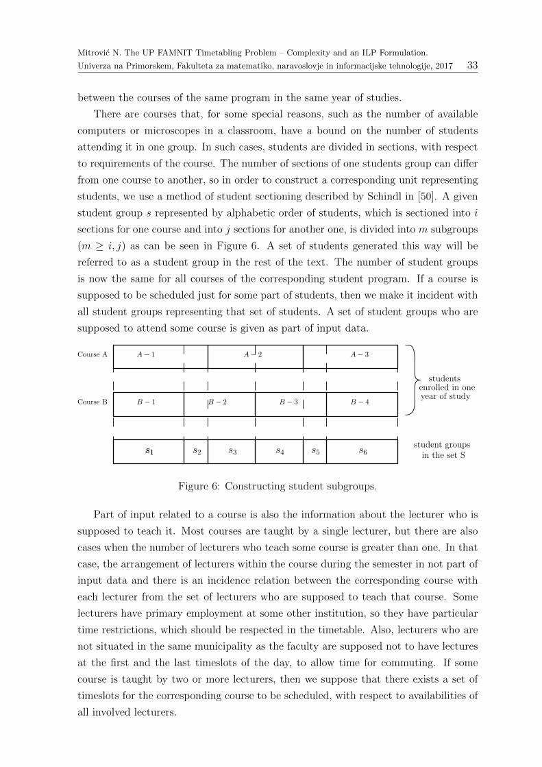
Mitrovic N. The UP FAMNIT Timetabling Problem – Complexity and an ILP Formulation.
Univerza na Primorskem, Fakulteta za matematiko, naravoslovje in informacijske tehnologije, 2017 33
between the courses of the same program in the same year of studies.
There are courses that, for some special reasons, such as the number of available
computers or microscopes in a classroom, have a bound on the number of students
attending it in one group. In such cases, students are divided in sections, with respect
to requirements of the course. The number of sections of one students group can differ
from one course to another, so in order to construct a corresponding unit representing
students, we use a method of student sectioning described by Schindl in [50]. A given
student group s represented by alphabetic order of students, which is sectioned into i
sections for one course and into j sections for another one, is divided into m subgroups
(m ≥ i, j) as can be seen in Figure 6. A set of students generated this way will be
referred to as a student group in the rest of the text. The number of student groups
is now the same for all courses of the corresponding student program. If a course is
supposed to be scheduled just for some part of students, then we make it incident with
all student groups representing that set of students. A set of student groups who are
supposed to attend some course is given as part of input data.
A− 1 A− 2 A− 3
B − 1 B − 2 B − 3 B − 4
Course A
Course B
studentsenrolled in oneyear of study
student groupss1 s2 s3 s4 s6s1 in the set S
s5
Figure 6: Constructing student subgroups.
Part of input related to a course is also the information about the lecturer who is
supposed to teach it. Most courses are taught by a single lecturer, but there are also
cases when the number of lecturers who teach some course is greater than one. In that
case, the arrangement of lecturers within the course during the semester in not part of
input data and there is an incidence relation between the corresponding course with
each lecturer from the set of lecturers who are supposed to teach that course. Some
lecturers have primary employment at some other institution, so they have particular
time restrictions, which should be respected in the timetable. Also, lecturers who are
not situated in the same municipality as the faculty are supposed not to have lectures
at the first and the last timeslots of the day, to allow time for commuting. If some
course is taught by two or more lecturers, then we suppose that there exists a set of
timeslots for the corresponding course to be scheduled, with respect to availabilities of
all involved lecturers.
Mitrovic N. The UP FAMNIT Timetabling Problem – Complexity and an ILP Formulation.
Univerza na Primorskem, Fakulteta za matematiko, naravoslovje in informacijske tehnologije, 2017 34
For every course there is a parameter representing the number of required hours on
a weekly level. The corresponding lecturer has the possibility to determine the division
of hours in blocks with respect to his/her desire. For example, a course taking four
hours per week can be taught either in one block of four hours, or in two blocks of two
hours, etc. In this way the number of occurrences of some course on the week level
is specified, as well as the number of required consecutive hours for each occurrence.
Note that if there is more than one lecturer teaching some course, all lecturers incident
with that course are assumed to agree on the desired division of the course.
The next resource to be described are classrooms. Availability of the classrooms is
known by the administrative sector of the institution and available as part of input.
Some of the classrooms are available without any restriction, while for some other this
is not the case. Also, some classrooms are available, but for an additional cost, or are
undesired for some other reasons, so their usage should be minimised. Classrooms are
of three types: regular classrooms, computer classrooms, and laboratory classrooms.
In the later two cases additional information is available, such as number of comput-
ers, number of microscopes, etc. Courses having requirements for special classroom
equipment should be assigned to an appropriate classroom. Respecting the classroom
capacity in the number of students attending some course is also obvious. Note that
large classrooms should be occupied most of the time, since just few of available class-
rooms have large capacities and the number of large student groups is not too small.
Not all buildings containing classrooms are located in the same town, so distance be-
tween them should be respected when preparing the timetable. We will say that two
classrooms are at the same location if both classrooms are in the same town. It is de-
sirable for a student group not to have lectures at more than one location at the same
day. One more obvious restriction concerning classrooms is that consecutive hours of
one course are supposed to be scheduled into the same classroom.
The requirements described above are more or less common for many similar insti-
tutions in the world. There are also some more specific things that have big influence
on the final result of the timetable structure. The first of them concerns upper bounds
on the number of teaching hours for teaching staff at day level. Parameters represent-
ing maximal number of teaching hours are determined with respect to type of course.
For example, one lecturer, say `, cannot teach more than ρL(`) timeslots per day of
courses being classified to be of type “lectures”. At the same time, the same person
cannot teach more that ρ(`) hours per day in total, not regarding the type of the
course. Upper bounds on the number of teaching hours per day for student groups are
also given, but do not represent a strict bound, just a preference.
The second special requirement describes the nature of lectures for master’s stu-
dents of some programmes: since the percentage of employed students enrolled in some
Mitrovic N. The UP FAMNIT Timetabling Problem – Complexity and an ILP Formulation.
Univerza na Primorskem, Fakulteta za matematiko, naravoslovje in informacijske tehnologije, 2017 35
programmes is very big, it is desirable to have teaching classes at afternoon hours, since
otherwise such students would not be able to attend. Also, there are periodical research
seminars for some of the departments at fixed time and place, so in the corresponding
timeslots teaching staff from the respective departments should not be assigned teach-
ing. The same holds for student groups who are supposed to attend research seminars.
Restrictions of this type also influence availability of some classrooms and this fact
should be considered when modelling the problem. The institution offers courses for
some study programmes of another institution, which have interdisciplinary character.
Teaching sessions relevant to these courses should be scheduled early in the morning,
or in the late afternoon, but not both in the same day, concerning one student group.
We define a meeting to be the main unit for timetabling. A meeting m is an
order pair consisting of a course c as the first coordinate, and a set of incident student
groups as the second one. In such a way a course that has to appear more than once,
for distinct sets of student groups, is represented by a few meetings, where each of
them is related to some of the corresponding set of student groups. For example, if a
course c is supposed to be scheduled for student groups s1 and s2 separately, then we
consider two meetings: m1 = (c, s1) and m2 = (c, s2). For every meeting the set of
lecturers incident with the meeting and the division into blocks are inherited from the
definition of the corresponding course.
Requirements for timetabling – summary
When preparing the timetable, there are requirements that should be respected. As al-
ready mentioned, hard constraints must be satisfied, while a violation of soft constraints
is allowed, but not desirable. In the following we list all hard and soft constraints rel-
evant for the considered institution.
Hard constraints
(i) Every meeting has to be assigned to available resources. The first re-
quirement of this type says that every meeting has to be assigned to an available
timeslot. Teachers are not available all the time, so they cannot have teach-
ing sessions at certain timeslots. Another type of time restriction included here
represents restrictions related to classrooms. Some classrooms are available all
the time, but some others are only available on specified timeslots. The third
requirement contained here is one determining acceptable classrooms for each
meeting. If a meeting has some specific requirement connected with equipment
of classroom, the requirement should be satisfied in order for the meeting to be
productive. Classrooms that satisfy requirements of meetings and capacities of
Mitrovic N. The UP FAMNIT Timetabling Problem – Complexity and an ILP Formulation.
Univerza na Primorskem, Fakulteta za matematiko, naravoslovje in informacijske tehnologije, 2017 36
student groups are determined by the student sector of the institution.
(ii) Overlapping is not permitted. A given student group cannot be assigned
to more than one meeting or to more than one classroom at a time. A similar
constraint holds for lecturers. Also, every classroom is allowed to be assigned at
most one meeting per timeslot.
(iii) The timetable has to be complete. All hours of each meeting have to be as-
signed to the timetable, with respect to division into blocks according to lecturers
decision. The hours of one meeting contained in one day have to be scheduled
consecutively and in the same classroom.
(iv) Pre-scheduled meetings. Some meetings and research seminars have prede-
fined times and classrooms. Students and teaching staff related to such events
should have an appropriate schedule allowing them to attend such events.
(v) Upper bounds on the number of hours per lecturer. There are parameters
that determine the maximum number of hours one lecturer can teach per day,
with respect to different types of meetings, as well as an overall bound.
(vi) Students restrictions. A student group from another institution can have
lectures just in the early morning or in the late afternoon timeslots, with an
additional requirement that both options are not allowed to happen at the same
time for the same student group. Students belonging to the same student group
cannot have meetings at two distinct locations in a day.
Soft constraints
(i) Minimal use of payable classrooms. As mentioned above, there are class-
rooms that can be used for teaching, but are payable. Since the use of such class-
rooms incurs additional costs, it is desirable to minimize the number of teaching
hours assigned to such classrooms.
(ii) Compact timetable and lunch break. For each student group, the meetings
corresponding to the group should be placed in the timetable without “big holes”,
as compactly as possible. If possible, it is desirable for students to have a lunch
break in the middle of the day.
(iii) Other student-related requirements. The amount of meetings should be
bounded in the sense that there is an upper bound on the number of teaching
hours on day level for every student group. Since many students are from other
parts of the country, it is desirable to minimize lectures on Friday afternoon.

Mitrovic N. The UP FAMNIT Timetabling Problem – Complexity and an ILP Formulation.
Univerza na Primorskem, Fakulteta za matematiko, naravoslovje in informacijske tehnologije, 2017 37
There are study programmes that are supposed to have teaching hours scheduled
only at afternoon slots.
4.2 Formal definition
In this section we give a formal definition of the timetabling problem for the described
institution based on requirements described in the previous section. Since soft con-
straints are just a measure for the quality of timetable and represent a part of the
objective function, they have no influence to the existence of a feasible solution. A
problem considered here is referred to as a Famnit Timetable Design, with respect
to hard constraints. This problem checks if there exists a feasible solution of the sys-
tem, i.e., a timetable that satisfies hard constraints. The Famnit Timetable Design
problem will be proved NP-complete in Chapter 5. For the formalization of hard and
soft constraints, see Sections 6.3 and 6.4 respectively.
Definition 4.1. The Famnit Timetable Design problem is defined as follows:
Instance:
• a finite set D of “days”;
• a finite set T of “timeslots” - set T is linearly ordered, so that first timeslot in a
week is the smallest element of T , and last timeslot in the week is the greatest
one; with respect to this ordering we define addition in T so that given a timeslot
t and a number i ∈ N, timeslot t′ = t+ i is defined as a timeslot being the (t+ i)-
th element of the linear order of set T (clearly, i cannot be arbitrarly large, we
discuss this in description of constraints);
• for each d ∈ D, a finite set T (d) ⊆ T of timeslots at day d ∈ D; clearly, the
family of sets T (d) defined this way represents a partition of set T ;
• a finite set M of “meetings”;
• a finite set S of “student groups”;
• a finite set L of “lecturers”;
• a finite set R of “rooms”;
• a finite set K of “locations”;
• a subset T (m) ⊆ T of available hours for each meeting m ∈M (for every meeting
the lecturer is known, so T (m) depends on lecturer availability);
Mitrovic N. The UP FAMNIT Timetabling Problem – Complexity and an ILP Formulation.
Univerza na Primorskem, Fakulteta za matematiko, naravoslovje in informacijske tehnologije, 2017 38
• a subset T (r) ⊆ T of available hours for each room r ∈ R;
• a subset M(s) ⊆M of meetings incident with each student subgroup s ∈ S;
• a subset M(`) ⊆M of meetings incident with each lecturer ` ∈ L;
• a subset R(m) ⊆ R of available rooms for each meeting m ∈M ;
• a subset M(k) ⊆M of meetings that take place at location k ∈ K;
• a multi-set P (m) of natural numbers; p ∈ P (m) if p hours of meeting m have to
be scheduled consecutively some time during the week;
• a number ρ(`) ∈ N for each lecturer ` ∈ L, the maximum number of hours ` can
teach per day;
• a finite set N of parts of a day (e.g. morning, noon, evening...); T (n) ⊆ T is the
set of all timeslots at n-th part of day d, over all d ∈ D;
• a set S ′ ⊆ S of student subgroups that can only have lectures within a single
part of a day;
• pre-scheduled things:
set G ⊆M × T ×R of pre-scheduled triples,
set F ⊆M × T ×R of triples that cannot be scheduled (unacceptable triples).
Question:
Is there a timetable that schedules all meetings, that is, a function f : M × T × R →{0, 1} (where f(m, t, r) = 1 means that meeting m is assigned to timeslot t and room
r) that schedules the desired number of hours of all meetings and satisfies the following
constraints.
1. Each meeting is scheduled to an acceptable timeslot:
∀m ∈M, ∀t ∈ T,∀r ∈ R : f(m, t, r) = 1⇒ t ∈ T (r) ∩ T (m).
2. Each meeting is assigned to a classroom that satisfies the requirements:
∀m ∈M,∀t ∈ T,∀r ∈ R : f(m, t, r) = 1⇒ r ∈ R(m).
3. Every meeting is assigned to at most one classroom at a time:
∀m ∈M, ∀t ∈ T,∀r1, r2 ∈ R : f(m, t, r1) = f(m, t, r2) = 1⇒ r1 = r2.
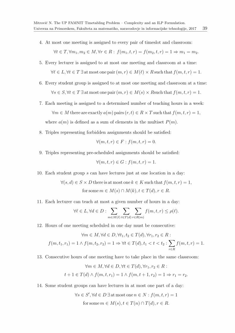
Mitrovic N. The UP FAMNIT Timetabling Problem – Complexity and an ILP Formulation.
Univerza na Primorskem, Fakulteta za matematiko, naravoslovje in informacijske tehnologije, 2017 39
4. At most one meeting is assigned to every pair of timeslot and classroom:
∀t ∈ T,∀m1,m2 ∈M,∀r ∈ R : f(m1, t, r) = f(m2, t, r) = 1⇒ m1 = m2.
5. Every lecturer is assigned to at most one meeting and classroom at a time:
∀` ∈ L,∀t ∈ T ∃ at most one pair (m, r) ∈M(`)×R such that f(m, t, r) = 1.
6. Every student group is assigned to at most one meeting and classroom at a time:
∀s ∈ S,∀t ∈ T ∃ at most one pair (m, r) ∈M(s)×Rsuch that f(m, t, r) = 1.
7. Each meeting is assigned to a determined number of teaching hours in a week:
∀m ∈M there are exactly a(m) pairs (r, t) ∈ R× T such that f(m, t, r) = 1,
where a(m) is defined as a sum of elements in the multiset P (m).
8. Triples representing forbidden assignments should be satisfied:
∀(m, t, r) ∈ F : f(m, t, r) = 0.
9. Triples representing pre-scheduled assignments should be satisfied:
∀(m, t, r) ∈ G : f(m, t, r) = 1.
10. Each student group s can have lectures just at one location in a day:
∀(s, d) ∈ S ×D there is at most one k ∈ K such that f(m, t, r) = 1,
for somem ∈M(s) ∩M(k), t ∈ T (d), r ∈ R.
11. Each lecturer can teach at most a given number of hours in a day:
∀` ∈ L,∀d ∈ D :∑
m∈M(`)
∑t∈T (d)
∑r∈R(m)
f(m, t, r) ≤ ρ(`).
12. Hours of one meeting scheduled in one day must be consecutive:
∀m ∈M,∀d ∈ D, ∀t1, t2 ∈ T (d),∀r1, r2 ∈ R :
f(m, t1, r1) = 1 ∧ f(m, t2, r2) = 1⇒ ∀t ∈ T (d), t1 < t < t2 :∑r∈R
f(m, t, r) = 1.
13. Consecutive hours of one meeting have to take place in the same classroom:
∀m ∈M,∀d ∈ D, ∀t ∈ T (d),∀r1, r2 ∈ R :
t+ 1 ∈ T (d) ∧ f(m, t, r1) = 1 ∧ f(m, t+ 1, r2) = 1⇒ r1 = r2.
14. Some student groups can have lectures in at most one part of a day:
∀s ∈ S ′,∀d ∈ D ∃ at most onen ∈ N : f(m, t, r) = 1
for somem ∈M(s), t ∈ T (n) ∩ T (d), r ∈ R.
Mitrovic N. The UP FAMNIT Timetabling Problem – Complexity and an ILP Formulation.
Univerza na Primorskem, Fakulteta za matematiko, naravoslovje in informacijske tehnologije, 2017 40
5 Proof of NP-completness
In Section 3.1 we mentioned the Timetable Design problem, which is known to be
NP-complete. In order to prove that Famnit Timetable Design is NP-complete,
we will apply Theorem 2.4 and show that it belongs to the class NP and that some
NP-complete problem polynomially reduces to it.
5.1 The problem is in NP
To see that the problem is in NP, we have to argue that for every yes instance I, there
exists a certificate with which the fact that I is a yes instance can be verified in time
polynomial in the size of input data. Such a certificate is naturally given by a timetable
that schedules all meetings, that is, a function f : M × T × R → {0, 1} satisfying the
constraints given in Definition 4.1. Thus, we can construct sets S1, S2 ⊆M×T×R such
that f takes value 1 on set S1 and 0 on set S2. Clearly, the verification of feasibility can
be done in polynomial time, since we have to check if f satisfies all constraints listed
in the definition. In the worst case we have to check all elements of the corresponding
index set determining some condition. That can be achieved in time polynomial in the
size of input data.
5.2 Reduction from an NP-complete problem
We showed that our problem is in NP. What remains is to prove that it is at least as
hard as some known NP-complete problem. The NP-complete problem used for this
proof is the Binary Timetable Design (BTD) problem defined in Section 3.1. We
construct a polynomial reduction R that reduces an instance I of the BTD problem
to an instance R(I) of Famnit Timetable Design (FTD) problem.
Recall that an instance of the BTD problem consists of a set C of craftsmen, a
set P of projects, a set H of work periods, subsets A(c), A(p) of H that represent
available work periods for craftsman c ∈ C and poject p ∈ P , respectively, and a
number R(c, p) ∈ {0, 1} of required work periods. In the following steps we construct
the reduction R.
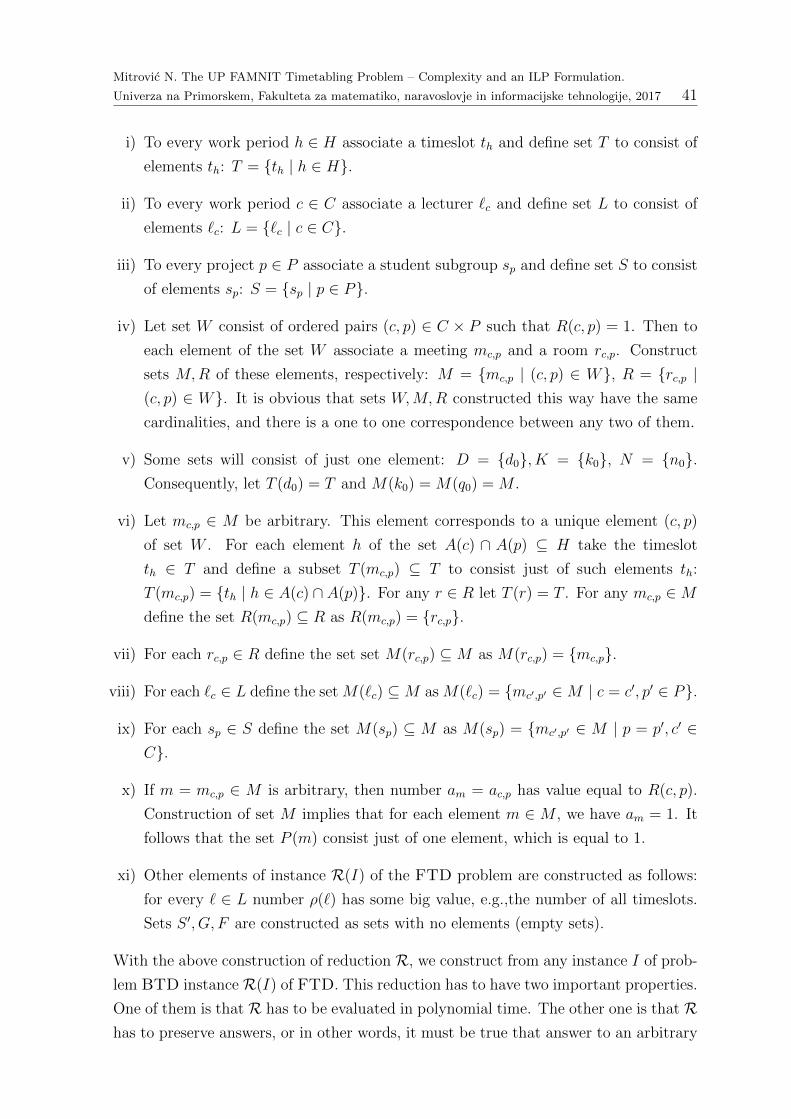
Mitrovic N. The UP FAMNIT Timetabling Problem – Complexity and an ILP Formulation.
Univerza na Primorskem, Fakulteta za matematiko, naravoslovje in informacijske tehnologije, 2017 41
i) To every work period h ∈ H associate a timeslot th and define set T to consist of
elements th: T = {th | h ∈ H}.
ii) To every work period c ∈ C associate a lecturer `c and define set L to consist of
elements `c: L = {`c | c ∈ C}.
iii) To every project p ∈ P associate a student subgroup sp and define set S to consist
of elements sp: S = {sp | p ∈ P}.
iv) Let set W consist of ordered pairs (c, p) ∈ C × P such that R(c, p) = 1. Then to
each element of the set W associate a meeting mc,p and a room rc,p. Construct
sets M,R of these elements, respectively: M = {mc,p | (c, p) ∈ W}, R = {rc,p |(c, p) ∈ W}. It is obvious that sets W,M,R constructed this way have the same
cardinalities, and there is a one to one correspondence between any two of them.
v) Some sets will consist of just one element: D = {d0}, K = {k0}, N = {n0}.Consequently, let T (d0) = T and M(k0) = M(q0) = M .
vi) Let mc,p ∈ M be arbitrary. This element corresponds to a unique element (c, p)
of set W . For each element h of the set A(c) ∩ A(p) ⊆ H take the timeslot
th ∈ T and define a subset T (mc,p) ⊆ T to consist just of such elements th:
T (mc,p) = {th | h ∈ A(c) ∩ A(p)}. For any r ∈ R let T (r) = T . For any mc,p ∈Mdefine the set R(mc,p) ⊆ R as R(mc,p) = {rc,p}.
vii) For each rc,p ∈ R define the set set M(rc,p) ⊆M as M(rc,p) = {mc,p}.
viii) For each `c ∈ L define the set M(`c) ⊆M as M(`c) = {mc′,p′ ∈M | c = c′, p′ ∈ P}.
ix) For each sp ∈ S define the set M(sp) ⊆ M as M(sp) = {mc′,p′ ∈ M | p = p′, c′ ∈C}.
x) If m = mc,p ∈ M is arbitrary, then number am = ac,p has value equal to R(c, p).
Construction of set M implies that for each element m ∈ M , we have am = 1. It
follows that the set P (m) consist just of one element, which is equal to 1.
xi) Other elements of instance R(I) of the FTD problem are constructed as follows:
for every ` ∈ L number ρ(`) has some big value, e.g.,the number of all timeslots.
Sets S ′, G, F are constructed as sets with no elements (empty sets).
With the above construction of reduction R, we construct from any instance I of prob-
lem BTD instance R(I) of FTD. This reduction has to have two important properties.
One of them is that R has to be evaluated in polynomial time. The other one is that Rhas to preserve answers, or in other words, it must be true that answer to an arbitrary
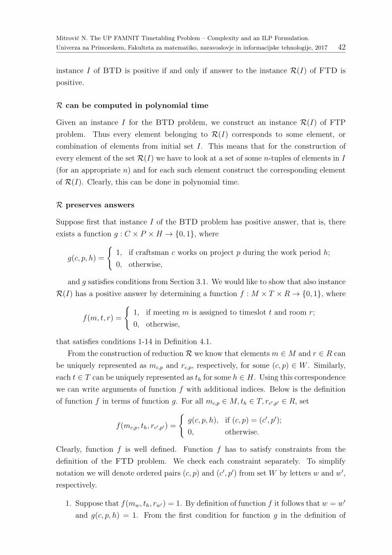
Mitrovic N. The UP FAMNIT Timetabling Problem – Complexity and an ILP Formulation.
Univerza na Primorskem, Fakulteta za matematiko, naravoslovje in informacijske tehnologije, 2017 42
instance I of BTD is positive if and only if answer to the instance R(I) of FTD is
positive.
R can be computed in polynomial time
Given an instance I for the BTD problem, we construct an instance R(I) of FTP
problem. Thus every element belonging to R(I) corresponds to some element, or
combination of elements from initial set I. This means that for the construction of
every element of the set R(I) we have to look at a set of some n-tuples of elements in I
(for an appropriate n) and for each such element construct the corresponding element
of R(I). Clearly, this can be done in polynomial time.
R preserves answers
Suppose first that instance I of the BTD problem has positive answer, that is, there
exists a function g : C × P ×H → {0, 1}, where
g(c, p, h) =
{1, if craftsman c works on project p during the work period h;
0, otherwise,
and g satisfies conditions from Section 3.1. We would like to show that also instance
R(I) has a positive answer by determining a function f : M × T ×R→ {0, 1}, where
f(m, t, r) =
{1, if meeting m is assigned to timeslot t and room r;
0, otherwise,
that satisfies conditions 1-14 in Definition 4.1.
From the construction of reductionR we know that elements m ∈M and r ∈ R can
be uniquely represented as mc,p and rc,p, respectively, for some (c, p) ∈ W . Similarly,
each t ∈ T can be uniquely represented as th for some h ∈ H. Using this correspondence
we can write arguments of function f with additional indices. Below is the definition
of function f in terms of function g. For all mc,p ∈M, th ∈ T, rc′,p′ ∈ R, set
f(mc,p, th, rc′,p′) =
{g(c, p, h), if (c, p) = (c′, p′);
0, otherwise.
Clearly, function f is well defined. Function f has to satisfy constraints from the
definition of the FTD problem. We check each constraint separately. To simplify
notation we will denote ordered pairs (c, p) and (c′, p′) from set W by letters w and w′,
respectively.
1. Suppose that f(mw, th, rw′) = 1. By definition of function f it follows that w = w′
and g(c, p, h) = 1. From the first condition for function g in the definition of
Mitrovic N. The UP FAMNIT Timetabling Problem – Complexity and an ILP Formulation.
Univerza na Primorskem, Fakulteta za matematiko, naravoslovje in informacijske tehnologije, 2017 43
Timetable Design problem it follows that h ∈ A(c) ∩ A(p). Reduction Rbijectively maps set T into H and set T (mw) into A(c) ∩ A(p), so it holds that
th belongs to T (mw), which is equal to T (mw) ∩ T (rw), since T (rw) = T .
2. Function f(mw, th, rw′) can have value 1 only if w = w′. But that means that
rw ∈ R(mw), so this constraint is satisfied.
3. Let mw ∈ M and th ∈ T and consider two rooms rw′ , rw′′ ∈ R such that
f(mw, th, rw′) = f(mw, th, rw′′) = 1. By definition of function f , it has to be
true that w = w′ and w = w′′, and so w′ = w′′. Hence elements rw′ and rw′′ are
equal, or in other words, there is at most one such element.
4. Let th ∈ T and rw ∈ R and suppose that there are two meetings mw′ ,mw′′ ∈ Msuch that f(mw′ , th, rw) = f(mw′′ , th, rw) = 1. By definition of function f , it
holds that w′′ = w = w′, so mw′ = mw′′ .
5. Let `c ∈ L and th ∈ T and consider two pairs (mw′ , rw′), (mw′′ , rw′′) ∈ M × R
such that mw′ ,mw′′ ∈ M(`c) and f(mw′ , th, rw′) = f(mw′′ , th, rw′′) = 1. Since
mw′ ,mw′′ ∈ M(`c), it follows from the construction of M(`c) that c′ = c′′, where
w′ = (c′, p′) and w′′ = (c′′, p′′). From the definition of f we have that g(c, p′, h) = 1
and g(c, p′′, h) = 1. But from the second constraint of g in the definition of
Timetable Design problem it follows that p′ = p′′, and because of that it holds
that w′ = w′′.
6. Let sp ∈ S and th ∈ T and consider two pairs (mw′ , rw′), (mw′′ , rw′′) ∈ M × Rsuch that mw′ ,mw′′ ∈ M(sp) and f(mw′ , th, rw′) = f(mw′′ , th, rw′′) = 1. Since
mw′ ,mw′′ ∈M(sp), from the construction of M(sp) it follows that p′ = p′′, where
w′ = (c′, p′) and w′′ = (c′′, p′′). Then from the definition of f we have that
g(c′, p, h) = 1 and g(c′′, p, h) = 1. But from the third constraint of g in definition
of Timetable Design problem it follows that c′ = c′′, and because of that it
holds that w′ = w′′.
7. Suppose that for a given meeting mc,p there are not exactly a(mc,p) = 1 pairs
(rc,p, th) such that f(mc,p, th, rc,p) = 1. Suppose first that there is no such pair.
Then f has value 0 for these arguments, and so g(c, p, h) = 0. This is in contra-
diction with the fourth condition of function g in the definition of Timetable
Design problem and definition of set M . Now suppose that there is more than
one such pair, say (rc,p, th′) and (rc,p, th′′), such that f(mc,p, th′ , rc,p) = 1 and
f(mc,p, th′′ , rc,p) = 1. What we get is that g(c, p, h′) = g(c, p, h′′) = 1, but this is
in contradiction with the fourth condition of function g, since we deal with the
binary version of the problem.
Mitrovic N. The UP FAMNIT Timetabling Problem – Complexity and an ILP Formulation.
Univerza na Primorskem, Fakulteta za matematiko, naravoslovje in informacijske tehnologije, 2017 44
8. The condition holds trivially since set F is the empty set.
9. The condition holds trivially since set G is the empty set.
10. The condition holds trivially since set K is a singleton.
11. The condition holds since by the definition of number ρ(l), the limit cannot be
exceeded.
12. This condition is trivially true, since the assumption of the condition is never
satisfied, that is, for every mw ∈M there is just one triple (mw, th, rw) such that
f(mw, th, rw) = 1.
13. Let mw ∈ M and th ∈ T . Suppose that f(mw, th, rw′) = f(mw, th + 1, rw′′) = 1,
where by th + 1 is denoted successor of the element th in linearly ordered set
T . Because of definition of the function f , it holds that w′ = w′′ = w and so
rw′ = rw′′ even without concerning consecutive timeslots.
14. This condition holds trivially since set S ′ is the empty set.
Since function f satisfies all conditions, it represents a feasible timetable, so instance
R(I) has positive answer.
Suppose now that the transformed instanceR(I) has positive answer to FTD problem.
We would like to derive that instance I also has positive answer to BTD problem. In
order to show this, we have to define a function g in terms of function f . This is done
as follows: for all c ∈ C, p ∈ P, h ∈ H, set
g(c, p, h) =
{f(mc,p, th, rc,p), if R(c, p) = 1,
0, otherwise.
Similarly as in the other direction of the proof, we have to show that function g describes
a feasible solution for the BTD problem, or more precisely that g satisfies conditions
from the definition of the Timetable Design problem.
1. Suppose that g(c, p, h) = 1. From the above formulation of g, it follows that
f(mc,p, th, rc,p) = R(c, p) = 1. The first condition of f gives that th ∈ T (rc,p) ∩T (mc,p) = T (mc,p), which corresponds to the set A(c) ∩ A(p).
2. Let h ∈ H and c ∈ C and consider two projects p′, p′′ ∈ P such that g(c, p′, h) =
g(c, p′′, h) = 1. Then it follows that also f(mc,p′ , th, rc,p′) = f(mc,p′′ , th, rc,p′′) = 1.
From the construction of set M(`c) it follows that mc,p′ ∈ M(`c), as well as
mc,p′′ ∈ M(`c). Condition 5 from the definition of FTD ensures that elements
mc,p′ and mc,p′′ are equal. Equality of p′ and p′′ follows.

Mitrovic N. The UP FAMNIT Timetabling Problem – Complexity and an ILP Formulation.
Univerza na Primorskem, Fakulteta za matematiko, naravoslovje in informacijske tehnologije, 2017 45
3. Let h ∈ H and p ∈ P and consider two craftsmen c′, c′′ ∈ C such that
g(c′, p, h) = g(c′′, p, h) = 1. Similarly as in the previous condition, we con-
clude that f(mc′,p, th, rc′,p) = f(mc′′,p, th, rc′′,p) = 1. But it also holds that both
elements (c′, p), and (c′′, p) are contained in set M(sp), and so condition 7 from
the definition of FTP problem ensures that these two elements are equal, and
consequently c′ = c′′.
4. If R(c, t) = 0, then obviously g(c, p, h) = 0 for all elements h ∈ H. Thus, assume
that R(c, t) = 1. Then also a(mc,p) = 1 and condition 7 from the definition
of FTD ensures that for each mc,p there is exactly one pair (rc′,p′ , th) so that
f(mc,p, th, rc′,p′) = 1. We see that (c, p) = (c′, p′), so this pair is fixed, and
argument th determines this pair, so element h is also unique.
Mitrovic N. The UP FAMNIT Timetabling Problem – Complexity and an ILP Formulation.
Univerza na Primorskem, Fakulteta za matematiko, naravoslovje in informacijske tehnologije, 2017 46
6 An integer programming
formulation
In this chapter we tie together things described in previous chapters and introduce
an integer linear program for the university timetabling problem at UP FAMNIT.
Consider the timetabling problem from Definition 4.1. We use the same terminology
as in Section 4.1.
6.1 Parameters of the ILP
Here we recall the structural elements introduced in the definition of Famnit
Timetable Problem and describe them in more detail. Note that in the
rest of this thesis we use simplified notation of some structural elements, so sets
T (d),M(`),M(s),M(k), R(m), T (`), T (r) are denoted by Td,M`,Ms,Mk, Rm, T`, Tr,
respectively.
• M is defined as the set of meetings to be assigned: every element m ∈ M is
an ordered pair containing a course as the first coordinate, and a set of student
subgroups as the second one. All meetings have a type determined: lectures or
tutorials. The set of meetings in M labelled as “lectures” or “tutorials” will be de-
noted by M lec and M tut, respectively. Obviously, M is the disjoint union of these
two sets. An example of element m ∈ M is an ordered pair (Course 1, {s1, s2}).For any meeting, lecturer and number of hours of the meeting to be assigned
are known, so for meeting m, number of hours per week is am. Any meeting m
is divided in parts, with respect to lecturers’ desire. These parts will be called
blocks. So for any meeting m there is a vector pm, with element pm(i) = k, if
a block of duration i of meeting m has to be repeated k times per week. For
any meeting m it holds that∑
i pm(i) · i = am. For any meeting m we define a
set Hm to be the set of all block lengths appearing in the division of meeting m,
i.e., Hm = {i | pm(i) 6= 0}. Let us introduce a short example: let meeting m
with am = 5 be separated in two blocks, with durations of 2 and 3 hours, respec-
tively. Such a division is denoted as (2 + 3). Then the corresponding vector is
pm = (0, 1, 1) and so Hm = {2, 3}. Another way of division of meeting m is in

Mitrovic N. The UP FAMNIT Timetabling Problem – Complexity and an ILP Formulation.
Univerza na Primorskem, Fakulteta za matematiko, naravoslovje in informacijske tehnologije, 2017 47
two blocks of length 1 and one block of length 3, denoted by 1 + 1 + 3. In that
case we have pm = (2, 0, 1) and Hm = {1, 3}.
• L: the set of lecturers.
• D: the set of days in a week, D = {1, 2, 3, 4, 5}.
• R: the set of classrooms.
• T : the set of all timeslots in the week; each element t ∈ T is an ordered pair, t =
(d, h), where d and h represent day and timeslot within the day, respectively; in
this work timeslots are supposed to have length 60 minutes. As already mentioned
in Definition 4.1, T is linearly ordered set, with t < t′, where t = (d, h), t′ =
(d′, h′), if d < d′ or if d = d′ and h < h′. The set of timeslots belonging to day
d is denoted by the Td. The number of timeslots in one day is denoted by a
constant τ (hence h ∈ {1, . . . , τ}, so the number of all timeslots is 5τ). Given a
timeslot t = (d, h) and a number i, such that i ≤ τ−h, we have t+ i := (d, h+ i).
• K: the set of locations, in our example there are two locations, denoted by k1
(Izola – University Campus Livade) and k2 (Koper).
• S: the set of student groups.
• M`: the set of class meetings given by lecturer ` ∈ L.
• Ms: the set of class meetings of a group of students s ∈ S.
• Mk: the set of class meetings that have to take place at location k ∈ K, in
particular: Mk1 ,Mk2 ;
• Rm: the set of rooms that are acceptable for meeting m ∈ M . A classroom is
acceptable for a particular meeting m if it satisfies requirements connected with
equipment of classroom and if it has sufficient capacity. From this set we can
construct a set MR of ordered pairs (m, r) containing all acceptable combinations
of meetings m and rooms r: MR := {(m, r) | m ∈M, r ∈ Rm}.
• T`: the set of timeslots t ∈ T in which lecturer ` ∈ L can have lectures. Here few
conditions have to be included. First, individual requirements of lecturers are
reflected in this set. The first and the last timeslots in a day are not acceptable
for lecturers not situated in same municipality as the institution. If a lecturer
has another job, is a member of some committee, or has some other regular
obligations, these constraints are also assumed to included in the set T`. For
instance, every Monday at 10AM teaching staff of the Mathematics department

Mitrovic N. The UP FAMNIT Timetabling Problem – Complexity and an ILP Formulation.
Univerza na Primorskem, Fakulteta za matematiko, naravoslovje in informacijske tehnologije, 2017 48
should have the possibility to attend the Mathematical research seminar. In order
to make this possible, they should not have any teaching obligations at that time.
Similarly, every Monday at 4PM teaching staff of Department of Information
Sciences and Technologies (abbreviated as DIST) should have the possibility to
attend the DIST research seminar, so there are no teaching obligations for them
at that time.
• Tr: the set of timeslots t ∈ T in which a given classroom r ∈ R can be used.
• MDIST : set of the meetings given by lecturers researching in Department of
Information Sciences and Technologies – in order to make fewer overlapping with
DIST research seminar;
• MPM : the set of meetings that are supposed to be assigned at afternoon timeslots;
• TAM : the set of morning timeslots; denote the number of morning timeslots in a
day by τAM ;
• TPM : the set of afternoon timeslots; denote the number of afternoon timeslots in
a day by τPM ;
• TMAS: the set of timeslots for the Mathematical research seminar;
• TDIST : the set of timeslots for the DIST research seminar;
• SAK : the set of student groups consisting of students of external programs –
Applied Kinesiology students;
6.2 Variables of the ILP
In the integer linear program all variables are binary. There are three different sets of
variables and we list them in the following.
• x-variables: For every triple of a meeting m ∈M , a timeslot t ∈ T , and a room
r ∈ Rm that is acceptable for that meeting, there is one corresponding variable
xm,t,r. This variable takes value 1 if meeting m is scheduled at timeslot t in
classroom r, and 0 otherwise:
xm,t,r =
{1, if meeting m is scheduled at timeslot t in classroom r,
0, otherwise.
• y-variables: For every triple of a meeting m ∈M , a timeslot t ∈ T and a prede-
fined length i ∈ Hm of individual blocks of meeting m we define a variable ym,t,i.
Mitrovic N. The UP FAMNIT Timetabling Problem – Complexity and an ILP Formulation.
Univerza na Primorskem, Fakulteta za matematiko, naravoslovje in informacijske tehnologije, 2017 49
The variable takes value 1 if timeslot t is the first appearance of i consecutive
hours of m, and 0 otherwise:
ym,t,i =
{1, if timeslot t is first appearance of i consecutive hours of meeting m,
0, otherwise.
• z-variables: In the last set of variables are so called z-variables, auxiliary vari-
ables for modelling some hard and soft constraints. Given a constraint of type
p and the corresponding index set Ip, we define a variable zp,i for every i ∈ Ip.Values of such variables will be determined by description of corresponding con-
straint. These variables will appear in the modelling of hard constraints of type
F1 (Section 6.3) and soft constraints of types S2 and S3 (Section 6.4).
6.3 Constraints of the ILP
A) Every meeting has to be assigned to available resources:
A1) Lecturers cannot have lectures at unacceptable timeslots:∑m∈M`
∑t∈T\T`
∑r∈Rm
xm,t,r = 0 ∀` ∈ L.
A2) Classrooms can only be used at specified timeslots:∑(m,r)∈MR
∑t∈T\Tr
xm,t,r = 0, ∀r ∈ R.
A3) Every meeting has to take place in an acceptable classroom: this constraint is
already satisfied by definition of variables, since xm,t,r variables are defined just
for classrooms r ∈ R that satisfy classroom requirements for the meeting m ∈M .
B) Overlapping is not permitted
B1) For every student group at most one meeting and one classroom can be assigned
to every teaching period:∑m∈Ms
∑r∈Rm
xm,t,r ≤ 1 ∀s ∈ S,∀t ∈ T.
B2) Every member of the teaching staff shall be assigned at most one meeting and
one classroom at a time:∑m∈M`
∑r∈Rm
xm,t,r ≤ 1 ∀` ∈ L,∀t ∈ T.

Mitrovic N. The UP FAMNIT Timetabling Problem – Complexity and an ILP Formulation.
Univerza na Primorskem, Fakulteta za matematiko, naravoslovje in informacijske tehnologije, 2017 50
B3) Every classroom can be assigned to at most one meeting at a time:∑(m,r)∈MR
xm,t,r ≤ 1 ∀r ∈ R, ∀t ∈ T.
C) Timetable has to be complete:
C1) All meetings in the curriculum of each student subgroup should be in the
timetable and in the right amount of teaching periods, with respect to weekly
duration: ∑t∈T
∑r∈Rm
xm,t,r = am ∀m ∈M.
C2) A meeting m of duration i ∈ Hm has to start and finish at the same day, so some
variables ym,t,i are defined to have value 0:
ym,t,i = 0 ∀m ∈M, ∀i ∈ Hm, ∀t = (d, h) ∈ T s.t. h > τ − i+ 1.
Recall that the parameter τ represents the number of timeslots in a day.
C3) Given a meeting m, at most one timeslot can be the first appearance of m in a
single day: ∑i∈Hm
∑t∈Td
ym,t,i ≤ 1, ∀m ∈M, ∀d ∈ D.
C4) A given meeting m of duration i (where i is the index of a nonzero element of
vector pm) has to appear exactly pm(i) times per week (i.e. in pm(i) days). All
such indices i are contained in set Hm, so we have:∑t∈T
ym,t,i = pm(i), ∀m ∈M, ∀i ∈ Hm.
C5) If a course m of duration i is assigned at day d, it has to be assigned to exactly
i hours:
i ·∑t∈Td
ym,t,i ≤∑r∈Rm
∑t∈Td
xm,t,r, ∀m ∈M,∀d ∈ D, ∀i ∈ Hm.
C6) Appearances of meeting m of duration i in a single day should be consecutive:
ym,t,i ≤∑r∈Rm
xm,t+j,r, ∀t = (d, h) ∈ T,∀m ∈M,∀i ∈ Hm,∀j = 0, . . . , i− 1,
where for t = (d, h), such that h+ j ≤ τ we have t+ j := (d, h+ j).
C7) All consecutive hours of one meeting should take place in the same classroom:
xm,t,r + xm,t+1,r′ ≤ 1 ∀m ∈M, ∀t ∈ T, ∀r, r′ ∈ Rm s.t. r 6= r′.
Mitrovic N. The UP FAMNIT Timetabling Problem – Complexity and an ILP Formulation.
Univerza na Primorskem, Fakulteta za matematiko, naravoslovje in informacijske tehnologije, 2017 51
D) Pre-scheduled meetings:
D1) There are activities at the Faculty that do not belong to the course offer. Such
activities represent pre-scheduled meetings, which should be scheduled to already
determined pairs of timeslots and classrooms. If a meeting is related to some
lecturers or students groups, their regular course meetings are undesirable at
that time. In particular, Research seminar at Mathematics’ department have to
be assigned to Monday, 10AM, in one specified room, call it r1. Hence, that room
is unavailable for other lectures at that time. Also, the DIST research seminar
has to be assigned to Monday, 4PM, in an already defined room, r2.1∑m∈M
∑t∈TMAS
xm,t,r1 = 0∑m∈M
∑t∈TCSS
xm,t,r2 = 0
D2) Meetings appearing as first coordinates of elements in set G have predetermined
timeslot and classrooms:
xm,t,r = 1, ∀(m, t, r) ∈ G.
E) Upper bounds on number of hours at day level
E1) It is not desired for lecturer ` to have more than ρ` timeslots of teaching obliga-
tions per day: ∑t∈Td
∑m∈M`
∑r∈Rm
xm,t,r ≤ ρ`, ∀` ∈ L, ∀d ∈ D.
There are also upper bounds with respect to meeting type, here we define it
parametrically as ρ1 and ρ2 for types “lectures” and “tutorials”, respectively.∑t∈Td
∑m∈M`∩M lec
∑r∈Rm
xm,t,r ≤ ρ1, ∀` ∈ L, ∀d ∈ D,
∑t∈Td
∑m∈M`∩Mtut
∑r∈Rm
xm,t,r ≤ ρ2, ∀` ∈ L, ∀d ∈ D.
Also, one more condition can be introduced, specifying that the lecturers shall
not have more than δ timeslots of teaching in every block of ∆ timeslots per day.
∆−1∑j=0
∑m∈M`
∑r∈Rm
xc,t+j,r ≤ δ ∀` ∈ L, ∀t = (d, h) ∈ T s.t. h ≤ τ −∆
1These activities are also related to a subset of teaching staff; however, these requirements are
already included in the definition of time availability of lecturers, T`.
Mitrovic N. The UP FAMNIT Timetabling Problem – Complexity and an ILP Formulation.
Univerza na Primorskem, Fakulteta za matematiko, naravoslovje in informacijske tehnologije, 2017 52
This type of constraints assures, for example, that for every lecturer, every period
of ∆ timeslots of teaching is preceded and followed by a break of length at least
∆− δ timeslots.
F) Student requirements
F1) Students of external interdisciplinary programmes should have lectures just in the
morning, or in the evening, but not both. So one of the following two conditions
has to be true, for every day and every student group belonging to external
programmes. This constraint checks if some meeting happens in some part of
day, so it is enough to check if some of corresponding y-variables has value 1.
Thus, these constraints are modelled using y-variables:∑m∈Ms
∑t∈Td\TAM
∑i∈Hm
ym,t,i ≤ 0 ∀d ∈ D, ∀s ∈ SAK∑m∈Ms
∑t∈Td\TPM
∑i∈Hm
ym,t,i ≤ 0 ∀d ∈ D, ∀s ∈ SAK .
In such a case at least one of two conditions has to be satisfied and we introduce a
variable zp,i, i ∈ Ip, as discussed in Section 2.3.1 (IV). Since p represents the type
of the constraint, for simplicity we will define p for this constraint to be equal to
F1. IF1 is the corresponding index set, in this case defined as I = SAK × D, so
the corresponding variable has indices zF1,s,d, for all (s, d) ∈ IF1 .
Constants B1 and B2 are chosen to have sufficiently large values. In this case, we
put both of them to be equal to 2, since it holds that all together in one day it
is not desired for students of Applied Kinesiology programme to have more than
two different meetings. Finally, the constraints are represented by the following
inequalities: ∑m∈Ms
∑t∈Td\TAM
∑i∈Hm
ym,t,i ≤ 2 · zF1,s,d ∀d ∈ D, ∀s ∈ SAK ,∑m∈Ms
∑t∈Td\TAM
∑i∈Hm
ym,t,i ≤ 2 · (1− zF1,s,d) ∀d ∈ D, ∀s ∈ SAK .
F2) It is desired for every student subgroup not to have meetings at two distinct
locations in a day:∑i∈Hm
ym,t,i +∑i∈Hm′
ym′,t′,i ≤ 1, ∀d ∈ D, ∀s ∈ Sk1 , ∀{t, t′} ∈ Td,
∀m ∈Mk1 ∩Ms,∀m′ ∈Mk2 ∩Ms.
Mitrovic N. The UP FAMNIT Timetabling Problem – Complexity and an ILP Formulation.
Univerza na Primorskem, Fakulteta za matematiko, naravoslovje in informacijske tehnologije, 2017 53
6.4 Soft constraints
Among the implicitly generated feasible solutions, we would like to get the best one.
In order to do that, we define an objective function, and an optimal solution is one
that will give the minimal value to the objective function. If some soft constraint is
violated, then the objective function value will grow. Soft constraints will be included in
the objective function as the sum of relevant variables, multiplied by the corresponding
weights. If a soft constraint of type p cannot be included in the objective function using
x- and y- variables, it will be modelled using z-variables, namely zp,i, for every i ∈ Ip,where Ip is the index set relevant for constraints of type p. In this section we introduce a
representation of each soft constraint in order to construct the corresponding variables.
Given a constraint of type p, variable zp,i, if exists, has following definition:
zp,i =
{1, if constraint of type p is not satisfied for element i of the index set Ip,
0, otherwise.
(6.1)
From equation (6.1) it follows that a violation of the constraint of type p, for some
i ∈ Ip, can be represented by a penalty term in the objective function, defined as
wizp,i, where wi is some positive weight. Obviously, a positive penalty increases the
value of the objective function, so solutions containing violated soft constraints will
have a larger value of the objective function.
The soft constraints are formalized as follows:
S1) Minimize use of payable classrooms. Some classrooms are available for
lecturing, but for an additional payment. It is desired to minimize the use of
such classrooms. This constraint can be represented using existing variables, by
adding element (6.2) to the objective function. Given a classroom r ∈ R and
a timeslot t ∈ T , we denote by wS1,r,t the “cost” of using classroom at timeslot
t. Observe that the weight wS1,r,t depends on the choice of the room r and the
timeslot t. In the case of UP FAMNIT the timeslot t has no influence to the
weight value at the time of this writing, although weights defined by both indices
are more general and can easily be adopted in case that choice of timeslot becomes
important for the cost of classroom. A constraint is represented by:∑r∈R
∑t∈Tr
∑m∈M
wS1,r,t · xm,t,r. (6.2)
S2) Compact timetable. Timetable compactness can have more forms. One of
them is from the lecturers’ point of view. This constraint is related to grouping
of teaching obligations of teaching staff, since it is not desirable for one teacher
to have some teaching hours in the morning and then again at the evening,
Mitrovic N. The UP FAMNIT Timetabling Problem – Complexity and an ILP Formulation.
Univerza na Primorskem, Fakulteta za matematiko, naravoslovje in informacijske tehnologije, 2017 54
with a long break in between. Since the number of teachers who teach just
one course, that is, who are incident just with one meeting, is not too small,
here it makes sense to refer just to teachers teaching more than one session.
Denote set of corresponding teachers by L+. Then we introduce binary variable
zS2,`,d, for every (`, d) ∈ L+ ×D, where S2 represents the type of constraint. As
already mentioned, sets TAM and TPM represent morning and afternoon timeslots,
respectively. Constraints representing S2 are the following:∑m∈M`
∑t∈Td∩TPM
∑r∈Rm
xm,t,r ≤ 0, ∀d ∈ D, ∀` ∈ L+,∑m∈M`
∑t∈Td∩TAM
∑r∈Rm
xm,t,r ≤ 0, ∀d ∈ D, ∀` ∈ L+.
Using variables zS2,l,d we get:∑m∈Ml
∑t∈Td∩TPM
∑r∈Rm
xm,t,r ≤ B1zS2,`,d, ∀d ∈ D, ∀` ∈ L+,∑m∈M`
∑t∈Td∩TAM
∑r∈Rm
xm,t,r ≥ B2(zS2,`,d − 1), ∀d ∈ D, ∀` ∈ L+.
Constants B1 and B2 have to have sufficiently large values. In this case it is
sufficient for them to be equal to the number of morning and afternoon timeslots
in a day, respectively. Thus, we define B1 and B2 to have values τPM and τAM ,
respectively.
For every variable zS2,`,d there is also a corresponding weight wS2,`,d used in ob-
jective function: ∑`∈LG
∑d∈D
wS2,`,d · zS2,`,d. (6.3)
S3) Requirements related to students. As mentioned in the description of the
teaching process at the institution, there are some Master’s study programmes
that are supposed to offer lectures just at afternoons timeslots. Meetings relevant
to these programmes belong to the set MPM , and number of such meetings sched-
uled for earlier timeslots should be minimised. Timeslots defined as afternoon
timeslots are contained in the set TPM ⊂ T . If it is not possible to put all meet-
ings from MPM in afternoon slots, there can be some measure that decides which
of the requirements are preferred to be satisfied. For that reason we introduce
weights wS3,m for every meeting m ∈ MPM , describing the importance of meet-
ing. A greater weight means that the course is more desirable to be scheduled in
the afternoon. The number of undesirable assignments is minimized by adding
the following element to the objective function:∑m∈MPM
∑t∈T\TPM
∑i∈Hm
wS3,m · ym,t,i. (6.4)
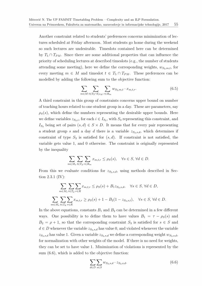
Mitrovic N. The UP FAMNIT Timetabling Problem – Complexity and an ILP Formulation.
Univerza na Primorskem, Fakulteta za matematiko, naravoslovje in informacijske tehnologije, 2017 55
Another constraint related to students’ preferences concerns minimization of lec-
tures scheduled at Friday afternoon. Most students go home during the weekend
so such lectures are undesirable. Timeslots contained here can be determined
by T5 ∩ TPM . Since there are some additional properties that can influence the
priority of scheduling lectures at described timeslots (e.g., the number of students
attending some meeting), here we define the corresponding weights, wS3,m,t, for
every meeting m ∈ M and timeslot t ∈ T5 ∩ TPM . These preferences can be
modelled by adding the following sum to the objective function:∑m∈M
∑t∈T5∩TPM
∑r∈Rm
wS3,m,t · xm,t,r. (6.5)
A third constraint in this group of constraints concerns upper bound on number
of teaching hours related to one student group in a day. These are parameters, say
ρS(s), which define the numbers representing the desirable upper bounds. Here
we define variables zS3,i, for each i ∈ IS3 , with S3 representing this constraint, and
IS3 being set of pairs (s, d) ∈ S × D. It means that for every pair representing
a student group s and a day d there is a variable zS3,s,d, which determines if
constraint of type S3 is satisfied for (s, d). If constraint is not satisfied, the
variable gets value 1, and 0 otherwise. The constraint is originally represented
by the inequality∑m∈Ms
∑t∈Td
∑r∈Rm
xm,t,r ≤ ρS(s), ∀s ∈ S, ∀d ∈ D.
From this we evaluate conditions for zS3,s,d, using methods described in Sec-
tion 2.3.1 (IV):∑m∈Ms
∑t∈Td
∑r∈R
xm,t,r ≤ ρS(s) +B1zS3,s,d, ∀s ∈ S, ∀d ∈ D,
∑m∈Ms
∑t∈Td
∑r∈R
xm,t,r ≥ ρS(s) + 1−B2(1− zS3,s,t), ∀s ∈ S, ∀d ∈ D.
In the above equations, constants B1 and B2 can be determined in a few different
ways. One possibility is to define them to have values B1 = τ − ρS(s) and
B2 = ρ + 1, so that the corresponding constraint S3 is satisfied for s ∈ S and
d ∈ D whenever the variable zS3,s,d has value 0, and violated whenever the variable
zS3,s,d has value 1. Given a variable zS3,s,d we define a corresponding weight wS3,s,d,
for normalization with other weights of the model. If there is no need for weights,
they can be set to have value 1. Minimization of violations is represented by the
sum (6.6), which is added to the objective function:∑d∈D
∑s∈S
wS3,s,d · zS3,s,d. (6.6)
Mitrovic N. The UP FAMNIT Timetabling Problem – Complexity and an ILP Formulation.
Univerza na Primorskem, Fakulteta za matematiko, naravoslovje in informacijske tehnologije, 2017 56
S4) Requirements related to lecturers. In Section 4.2 we defined sets T (`), for
each ` ∈ L, representing available timeslots for lecturer `. Even if timeslots are
contained in the set T (`), there are some of them that might be preferred by the
lecturer. For that reason we introduce a soft constraint representing a measure of
lecturers’ preferences with respect to the timeslots that are assigned to teaching
hours. For each pair of lecturer ` ∈ L and timeslot t ∈ T (`) we define a weight
wS4,`,t representing the measure of preferences. A modelled constraint has the
form: ∑`∈L
∑m∈M(`)
∑t∈T
∑r∈Rm
wS4,`,t · xm,t,r.
6.5 The objective and the size of the ILP
Putting together the sums described above, we can formulate the objective function of
the ILP model as follows:∑t∈Tr
∑m∈M
∑r∈Rm
wS1,r,t · xm,t,r +∑`∈L+
∑d∈D
wS2,`,d · zS2,`,d+∑m∈MPM
∑t∈T\TPM
∑i∈Hm
wS3,m · ym,t,i +∑m∈M
∑t∈T5∩TPM
∑r∈Rm
wS3,m,t · xm,t,r+∑d∈D
∑s∈S
wS3,s,d · zS3,s,d +∑`∈L
∑m∈M(`)
∑t∈T
∑r∈Rm
wS4,`,t · xm,t,r.
For notational clarity, in this section we denote the cardinalities of sets
L,L+,M,R, S, SAK , T, Td, G by λ, λ+, µ, ρ, σ, σAK , θ, τ, γ, respectively. The number of
blocks of distinct lengths for each meeting m ∈M is denoted by ω(m), while ρ(m) and
µ(s) denote the number of rooms that are acceptable for meeting m, and the number
of meetings incident with student group s, respectively. Note that, as there are 5 days
belonging to set D, we have θ = 5τ . In total, the number of variables of described ILP
is equal to
µθρ+ µθ∑m∈M
ω(m) + 2δσ + δλ.
The numbers of x-, y- and z-variables is represented in Table 2. Computing the number
of constraints is not that trivial. In Table 3 we list the number of constraints grouped
by constraint type. The total number of constraints in the ILP is equal to the sum of
all terms displayed in the right column of Table 3.
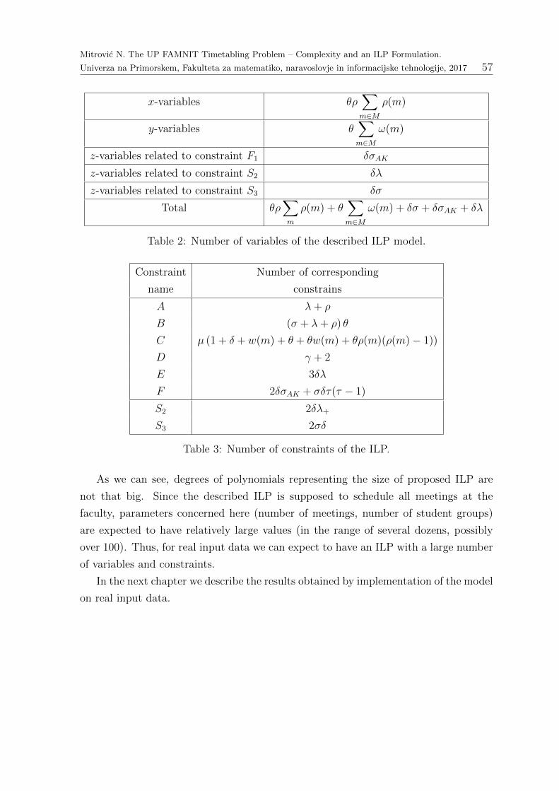
Mitrovic N. The UP FAMNIT Timetabling Problem – Complexity and an ILP Formulation.
Univerza na Primorskem, Fakulteta za matematiko, naravoslovje in informacijske tehnologije, 2017 57
x-variables θρ∑m∈M
ρ(m)
y-variables θ∑m∈M
ω(m)
z-variables related to constraint F1 δσAK
z-variables related to constraint S2 δλ
z-variables related to constraint S3 δσ
Total θρ∑m
ρ(m) + θ∑m∈M
ω(m) + δσ + δσAK + δλ
Table 2: Number of variables of the described ILP model.
Constraint Number of corresponding
name constrains
A λ+ ρ
B (σ + λ+ ρ) θ
C µ (1 + δ + w(m) + θ + θw(m) + θρ(m)(ρ(m)− 1))
D γ + 2
E 3δλ
F 2δσAK + σδτ(τ − 1)
S2 2δλ+
S3 2σδ
Table 3: Number of constraints of the ILP.
As we can see, degrees of polynomials representing the size of proposed ILP are
not that big. Since the described ILP is supposed to schedule all meetings at the
faculty, parameters concerned here (number of meetings, number of student groups)
are expected to have relatively large values (in the range of several dozens, possibly
over 100). Thus, for real input data we can expect to have an ILP with a large number
of variables and constraints.
In the next chapter we describe the results obtained by implementation of the model
on real input data.
Mitrovic N. The UP FAMNIT Timetabling Problem – Complexity and an ILP Formulation.
Univerza na Primorskem, Fakulteta za matematiko, naravoslovje in informacijske tehnologije, 2017 58
7 Results
In this chapter we present results obtained using an implementation of the integer linear
programming model derived in Chapter 6. The model was implemented using the open
source programming software Zimpl, available from the web page http://zimpl.zib.de/,
with user manual described in [34], and evaluated using the Gurobi Optimization soft-
ware, available from the web page www.gurobi.com, with user manual contained in [42].
In what follows the Gurobi Optimization software will be referred to as a solver. The
specifications of computer used for the computations are: RAM 32GB DDR3 1800Mhz
and CPU: Intel i7-3820 3.60GHz.
In order to find an optimal solution of the proposed model, we used input data
for the Spring Semester of the academic year 2016/17 at the Faculty of Mathematics,
Natural Sciences and Information Technologies, University of Primorska. Regarding
these data, we have 185 meetings, 26 classrooms, and 65 timeslots. At the faculty
there are 17 distinct study programmes that in total define 48 student groups, while
the number of lecturers is equal to 118.
The timetable is supposed to be prepared for 5 working days and τ = 13 timeslots
within a day, each of them of the length equal to 60 minutes. Thus, in total there
are 65 timeslots in the week. For the concrete data we define values of parameters
introduced in the description of the model. We have: the overall upper bound on
number of teaching timeslots of lecturer `, ρL(`) = 8, for every lecturer ` ∈ L; upper
bounds with respect to meeting type, ρ1 = 6, ρ2 = 8. The upper bound regarding the
students’ requirements, ρS(s) is defined to have the value equal to 9, for every student
group s.
In Section 6.4 we introduced weights used for the formulation of the terms of objec-
tive function. These weights measure various criteria that are desired to be optimized
in order to define the quality of the timetable. The number of weights is too large,
so we do not list them here. All weights have values between 0 and 5. The objective
function is being minimized so a large penalty weight means that we would really like
corresponding variable to take value 0, meaning that the constraint is satisfied. This
way the objective function value grows when an undesired feature of the schedule is
present, since the corresponding weight multiplies by 1 and not by 0.
Using the Zimpl software we generated a .lp file representing the proposed model
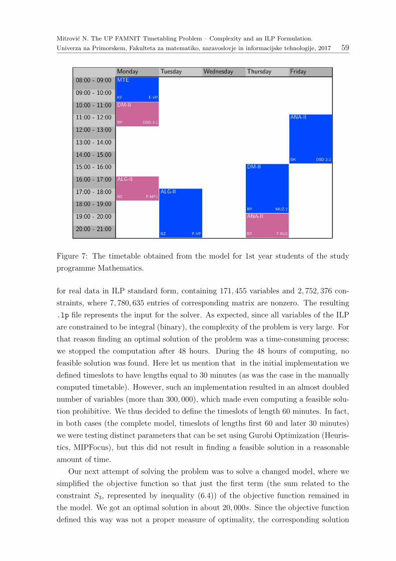
Mitrovic N. The UP FAMNIT Timetabling Problem – Complexity and an ILP Formulation.
Univerza na Primorskem, Fakulteta za matematiko, naravoslovje in informacijske tehnologije, 2017 59
Figure 7: The timetable obtained from the model for 1st year students of the study
programme Mathematics.
for real data in ILP standard form, containing 171, 455 variables and 2, 752, 376 con-
straints, where 7, 780, 635 entries of corresponding matrix are nonzero. The resulting
.lp file represents the input for the solver. As expected, since all variables of the ILP
are constrained to be integral (binary), the complexity of the problem is very large. For
that reason finding an optimal solution of the problem was a time-consuming process;
we stopped the computation after 48 hours. During the 48 hours of computing, no
feasible solution was found. Here let us mention that in the initial implementation we
defined timeslots to have lengths equal to 30 minutes (as was the case in the manually
computed timetable). However, such an implementation resulted in an almost doubled
number of variables (more than 300, 000), which made even computing a feasible solu-
tion prohibitive. We thus decided to define the timeslots of length 60 minutes. In fact,
in both cases (the complete model, timeslots of lengths first 60 and later 30 minutes)
we were testing distinct parameters that can be set using Gurobi Optimization (Heuris-
tics, MIPFocus), but this did not result in finding a feasible solution in a reasonable
amount of time.
Our next attempt of solving the problem was to solve a changed model, where we
simplified the objective function so that just the first term (the sum related to the
constraint S3, represented by inequality (6.4)) of the objective function remained in
the model. We got an optimal solution in about 20, 000s. Since the objective function
defined this way was not a proper measure of optimality, the corresponding solution
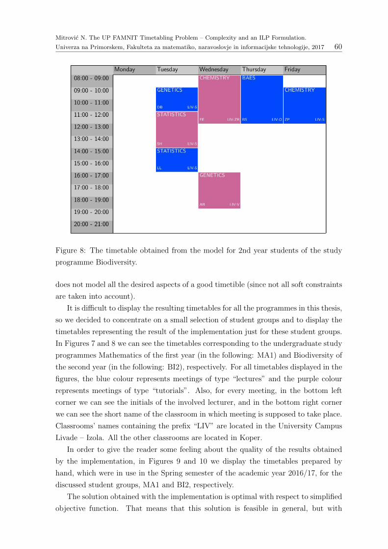
Mitrovic N. The UP FAMNIT Timetabling Problem – Complexity and an ILP Formulation.
Univerza na Primorskem, Fakulteta za matematiko, naravoslovje in informacijske tehnologije, 2017 60
Figure 8: The timetable obtained from the model for 2nd year students of the study
programme Biodiversity.
does not model all the desired aspects of a good timetible (since not all soft constraints
are taken into account).
It is difficult to display the resulting timetables for all the programmes in this thesis,
so we decided to concentrate on a small selection of student groups and to display the
timetables representing the result of the implementation just for these student groups.
In Figures 7 and 8 we can see the timetables corresponding to the undergraduate study
programmes Mathematics of the first year (in the following: MA1) and Biodiversity of
the second year (in the following: BI2), respectively. For all timetables displayed in the
figures, the blue colour represents meetings of type “lectures” and the purple colour
represents meetings of type “tutorials”. Also, for every meeting, in the bottom left
corner we can see the initials of the involved lecturer, and in the bottom right corner
we can see the short name of the classroom in which meeting is supposed to take place.
Classrooms’ names containing the prefix “LIV” are located in the University Campus
Livade – Izola. All the other classrooms are located in Koper.
In order to give the reader some feeling about the quality of the results obtained
by the implementation, in Figures 9 and 10 we display the timetables prepared by
hand, which were in use in the Spring semester of the academic year 2016/17, for the
discussed student groups, MA1 and BI2, respectively.
The solution obtained with the implementation is optimal with respect to simplified
objective function. That means that this solution is feasible in general, but with
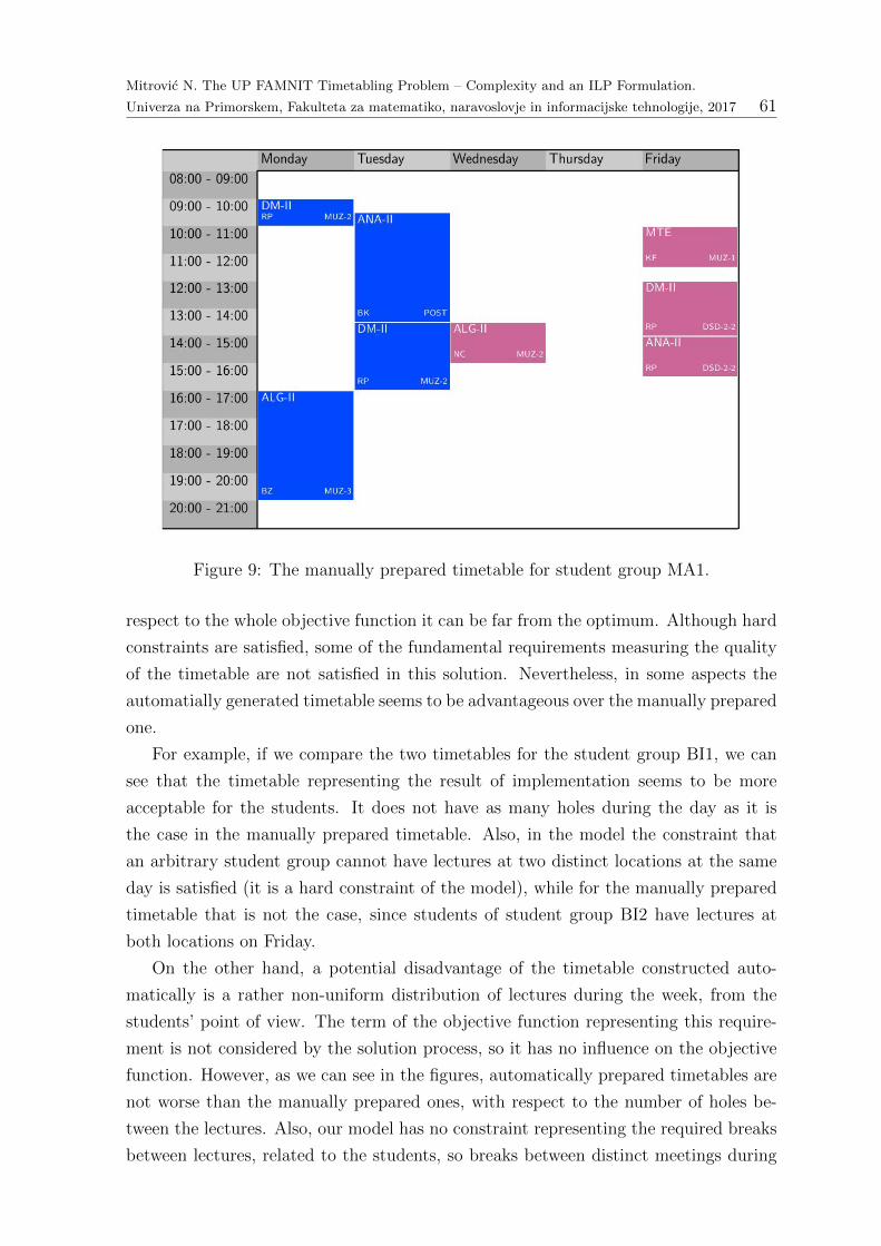
Mitrovic N. The UP FAMNIT Timetabling Problem – Complexity and an ILP Formulation.
Univerza na Primorskem, Fakulteta za matematiko, naravoslovje in informacijske tehnologije, 2017 61
Figure 9: The manually prepared timetable for student group MA1.
respect to the whole objective function it can be far from the optimum. Although hard
constraints are satisfied, some of the fundamental requirements measuring the quality
of the timetable are not satisfied in this solution. Nevertheless, in some aspects the
automatially generated timetable seems to be advantageous over the manually prepared
one.
For example, if we compare the two timetables for the student group BI1, we can
see that the timetable representing the result of implementation seems to be more
acceptable for the students. It does not have as many holes during the day as it is
the case in the manually prepared timetable. Also, in the model the constraint that
an arbitrary student group cannot have lectures at two distinct locations at the same
day is satisfied (it is a hard constraint of the model), while for the manually prepared
timetable that is not the case, since students of student group BI2 have lectures at
both locations on Friday.
On the other hand, a potential disadvantage of the timetable constructed auto-
matically is a rather non-uniform distribution of lectures during the week, from the
students’ point of view. The term of the objective function representing this require-
ment is not considered by the solution process, so it has no influence on the objective
function. However, as we can see in the figures, automatically prepared timetables are
not worse than the manually prepared ones, with respect to the number of holes be-
tween the lectures. Also, our model has no constraint representing the required breaks
between lectures, related to the students, so breaks between distinct meetings during
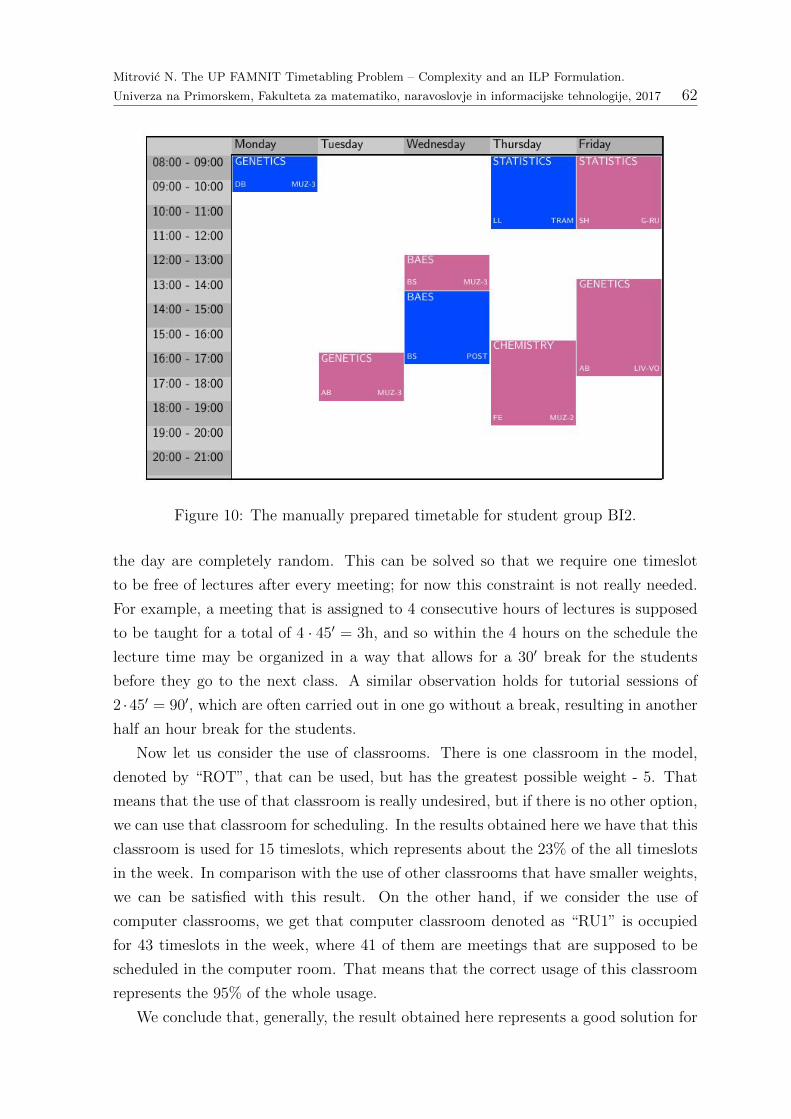
Mitrovic N. The UP FAMNIT Timetabling Problem – Complexity and an ILP Formulation.
Univerza na Primorskem, Fakulteta za matematiko, naravoslovje in informacijske tehnologije, 2017 62
Figure 10: The manually prepared timetable for student group BI2.
the day are completely random. This can be solved so that we require one timeslot
to be free of lectures after every meeting; for now this constraint is not really needed.
For example, a meeting that is assigned to 4 consecutive hours of lectures is supposed
to be taught for a total of 4 · 45′ = 3h, and so within the 4 hours on the schedule the
lecture time may be organized in a way that allows for a 30′ break for the students
before they go to the next class. A similar observation holds for tutorial sessions of
2 ·45′ = 90′, which are often carried out in one go without a break, resulting in another
half an hour break for the students.
Now let us consider the use of classrooms. There is one classroom in the model,
denoted by “ROT”, that can be used, but has the greatest possible weight - 5. That
means that the use of that classroom is really undesired, but if there is no other option,
we can use that classroom for scheduling. In the results obtained here we have that this
classroom is used for 15 timeslots, which represents about the 23% of the all timeslots
in the week. In comparison with the use of other classrooms that have smaller weights,
we can be satisfied with this result. On the other hand, if we consider the use of
computer classrooms, we get that computer classroom denoted as “RU1” is occupied
for 43 timeslots in the week, where 41 of them are meetings that are supposed to be
scheduled in the computer room. That means that the correct usage of this classroom
represents the 95% of the whole usage.
We conclude that, generally, the result obtained here represents a good solution for
Mitrovic N. The UP FAMNIT Timetabling Problem – Complexity and an ILP Formulation.
Univerza na Primorskem, Fakulteta za matematiko, naravoslovje in informacijske tehnologije, 2017 63
the timetabling problem (that is, a solution that could be used in the application). The
existence of a feasible solution represents a good first step in the process of automating
the approach to the timetabling problem at UP FAMNIT, as the number of variables is
large for relatively fast solving.1 A few steps have to be taken care of before a complete
automation of the process as until now the timetabling problem at UP FAMNIT was
solved manually. One of them is the preparation of the data for the model. Manual
timetabling allows to include a human note that breaks hard constraints in some sit-
uations in order to achieve a better overall result. However, it is difficult if not even
impossible to define the constraints in such a way to enable a computer program to
achieve the same results. There is no possibility for computer to think about “impor-
tance” of some of the hard constraints. Since the work of this thesis represents the first
attempt towards automation of the timetabling problem at UP FAMNIT, we expect
that some improvements with the more technical part of the whole process of solving
the problem will take place in the near future (priority: a simplified collecting of the
data).
The timetable constructed here could be used in the teaching process of the faculty,
with possibility of minor changes made by human, in order to make it even better.
For now, we will try to make further improvements to the model so that we can get a
solution with respect to the whole objective function in a reasonable amount of time.
The first task for future research is to reduce the number of binary variables and to
implement some terms of the objective function in a different way, so that we can at
least get a reasonably good solution for the whole model relatively quickly.
1We say that a solution is found relatively fast if it takes less time to find it using the proposed
model, than to construct it by hand.
Mitrovic N. The UP FAMNIT Timetabling Problem – Complexity and an ILP Formulation.
Univerza na Primorskem, Fakulteta za matematiko, naravoslovje in informacijske tehnologije, 2017 64
8 Conclusion
In the thesis we considered a university timetabling problem (UTP). The UTP can
have many definitions, depending on the resources that are supposed to be sched-
uled to time intervals. In this work we described the teaching process at the Faculty
of Mathematics, Natural Sciences and Information Technologies at University of Pri-
morska (UP FAMNIT). Based on that description, we formalized the definition of the
timetabling problem at UP FAMNIT, referred to as the Famnit Timetable Design
(FTD) problem, and proved that so defined problem is NP-complete.
Unless P 6= NP , the NP-completeness of the problem implies non-existence of an
efficient solution for the problem. Among the few approaches for modelling timetabling
problems, reviewed in Section 3.2, we decided to model the problem using concepts
of integer linear programming. We developed an ILP model representing the FTD
problem, consisting of binary variables, constraints representing requirements of the
faculty, and an objective function measuring the quality of feasible solutions.
The model proposed in this work is implemented for the real input data using the
relevant software. As already discussed, the number of binary variables of the ILP
is larger than 150, 000, so it is expected that solving the problem to optimality will
take a long time. For the given data we did not manage to get an optimal solution
of the complete ILP as described in Chapter 6. When solving the simplified ILP, or
more precisely the ILP with the same set of constraints and with the objective function
containing just one of the main terms, an optimal solution was found in a relatively
short time given the size of the problem. We can conclude that besides the large number
of binary variables, the objective function also has a big influence on the amount of
time needed to get an optimal solution.
One of the possible directions for the improvement of the ILP model developed in
thesis would be a reduction in the number of variables. One of the ideas of how to
do that is to discard variables with indices that are supposed to have value 0 (e.g.,
time availabilities of professors/classrooms could be respected during the initialization
of variables). Also, during the testing of developed model, we realized that there are
constraints that have a big influence on the amount of time needed to solve the problem,
so we believe that separating a problem into two subproblems, containing “weak” and
“hard” constraints,, respectively, could give us a good solution approach.
Mitrovic N. The UP FAMNIT Timetabling Problem – Complexity and an ILP Formulation.
Univerza na Primorskem, Fakulteta za matematiko, naravoslovje in informacijske tehnologije, 2017 65
9 Povzetek dela v slovenskem
jeziku
Problemi sestavljanja urnikov na univerzah so prakticni NP-tezki problemi, ki jih
je tezko resiti do optimalnosti. V literaturi je na voljo veliko razlicnih modelov za
tovrstne probleme, ki temeljijo na metodah teorije grafov, kombinatoricne optimizacije,
logicnega programiranja z omejitvami (ang. constraint logic programming) in/ali
celostevilskega (ali mesanega celostevilskega) programiranja. Modeli vodijo do opti-
malnih eksaktnih algoritmov eksponentne casovne zahtevnosti ali do hevristicnih algo-
ritmov polinomske casovne zahtevnosti. Sestavljanje urnika predstavlja zelo specificen
problem, ki je zelo odvisen od posebnosti pogojev, ki morajo veljati zanj. Zaradi tega ne
obstaja splosna resitev problema in je tezko algoritem oziroma model, ki je ze narejen
v literaturi, uporabiti v drugem konkretnem primeru.
V magistrskem delu je podan pregled pomembne in nedavne literature s podrocja,
povzeti so razlicni modeli in pristopi za resevanje problema urnika, s prednostimi in po-
manjkljivostmi. Podan je pregled nekaterih teoreticnih pojmov in rezultatov, povezanih
z racunsko zahtevnostjo problemov, kombinatoricno optimizacijo, linearnim programi-
ranjem in celostevilskim linearnim programiranjem. Tako so predstavljeni razredi kom-
pleksnosti problemov, kot so razred P, NP, ter razred NP-polnih problemov. Obstoj
NP-polnih problemov ni ociten, zato je v nalogi naveden rezultat, ki obstoj tovrstnih
problemov zagotavlja, znan kot Cookov izrek. Z uporabo Cookovega izreka in polinom-
skih prevedb problemov je podana karakterizacija NP-polnih problemov, ki bistveno
olajsa postopek dokazovanja NP-polnosti dolocenega problema.
Glede na to da je v delu problem univerzitetnega urnika modeliran z uporabo
celostevilskega linearnega programiranja, je nekaj strani namenjenih teoriji s tega po-
drocja. Podani so osnovni rezultati teorije linearnega programiranja, med katerimi so
najbolj znani Farkaseva lema in izrek o dualnosti linearnega programa. Definirano je
celostevilsko linearno programiranje, ki predstavlja enega izmed prvih dokazano NP-
polnih problemov. Razlozena je racunska zahtevnost celostevilskega linearnega pro-
gramiranja in razlicni pristopi za resevanje celostevilskih linearnih programov: ravnin-
ski rezi, metoda razveji-in-omeji, dinamicno programiranje itn.
S ciljem cim bolje razumeti problem, je v delu podana splosna definicija problema
Mitrovic N. The UP FAMNIT Timetabling Problem – Complexity and an ILP Formulation.
Univerza na Primorskem, Fakulteta za matematiko, naravoslovje in informacijske tehnologije, 2017 66
urnika, ter kratka razlaga njegove raunske zahtevnosti, saj je splosni problem urnika
dokazano NP-poln. Posebna pozornost je namenjena pregledu literature, ki se uk-
varja zgolj s problemom dolocitve urnika predavanj na univerzah. Pogoji, ki morajo
veljati za posamezen urnik, namrec lahko pomembno vplivajo na casovno zahtevnost
problema. V nalogi so predstavljeni primeri pogojev, pod katerimi je problem se vedno
resljiv v polinomskem casu, ter pogoji, ki zelo vplivajo na zvisanje racunske zahtevnosti
problema. Problem urnika oziroma njegove razlicice so natancno opisane, vkljucno z
vsemi spremenljivkami in omejitvami. Natancno je definirana posebna vrsta problema,
poimenovana Famnit Timetable Design (FTD), ki ustreza problemu urnika na
Fakulteti za matematiko, naravoslovje in informacijske tehnologije Univerze na Pri-
morskem (UP FAMNIT). Kot nov rezultat je izpeljan dokaz NP-polnosti FTD prob-
lema, in sicer s konstrukcijo polinomske prevedbe z ze znanega NP-polnega problema.
V drugem delu magistrskega dela je poudarek na izpeljavi matematicnega mod-
ela problema v obliki celostevilskega linearnega programa. Najprej so natancno
opisane podrobnosti izvajanja studijskega procesa na UP FAMNIT. Predstavljeni so
pogoji, ki morajo biti zadosceni pri pripravi urnika (t.i. trdi pogoji), ter pogoji, ki
so zazeljeni, vendar niso nujni za postavitev urnika (t.i. mehki pogoji). V poseb-
nem poglavju je opisan celostevilski linearen program za problem urnika na UP
FAMNIT, s spremenljivkami in pogoji. Program je implementiran z uporabo pro-
gramskega paketa Zimpl (prosto dostopnim na strani http://zimpl.zib.de/) in resen
na konkretnih primerih z uporabo programskega paketa Gurobi (dostopnim na strani
http://www.gurobi.com/).
Model je preizkusen na konkretnih podatkih, in sicer za fakultetni urnik za spom-
ladanski semester studijskega leta 2016/17. Zaradi velikega stevila spremenljivk je bilo
resevanje problema dolgotrajno. Dobljena resitev tako ni nujno optimalna, ampak le
dovolj blizu optimuma, oziroma predstavlja resitev, ki ima najboljso vrednost kriteri-
jske funkcije, dobljena v dolocenem (omejenem) casovnem intervalu. Dobljena resitev
je primerjana z rocno sestavljenim urnikom, tako da je za nekaj skupin studentov pred-
stavljen dejanski urnik predavanj na fakulteti za obravnavani semester in urnik, dobljen
kot rezultat implementacije in resevanja celostevilskega linearnega programa.
Opisan celostevilski linearen program vsebuje veliko stevilo bina-
rnih spremenljivk, ki zvisajo cas, potreben za resevanje problema, zato
je v zakljucku predlaganih nekaj idej za pospesitev resevanja programa,
v obliki zmanjsanja stevila spremenljivk in poenostavitve kriterijske
funkcije.
Mitrovic N. The UP FAMNIT Timetabling Problem – Complexity and an ILP Formulation.
Univerza na Primorskem, Fakulteta za matematiko, naravoslovje in informacijske tehnologije, 2017 67
10 Bibliography
[1] Slim Abdennadher and Michael Marte. University course timetabling using con-
straint handling rules. Applied Artificial Intelligence, 14(4):311–325, 2000. (Cited
on page 30.)
[2] Aderemi O. Adewumi, Babatunde A. Sawyerr, and Ali M. Montaz. A heuris-
tic solution to the university timetabling problem. Engineering Computations,
26(8):972–984, 2009. (Cited on page 29.)
[3] Nur A.H. Aizam and Louis Caccetta. Computational models for timetabling prob-
lems. Numerical Algebra, Control and Optimization, 4(1):269–285, 2014. (Cited
on page 28.)
[4] Ruibin Bai, Edmund K. Burke, Graham Kendall, and Barry McCollum. A sim-
ulated annealing hyper-heuristic for university course timetabling problem. In
International Conference on the Practice and Theory of Automated Timetabling,
Abstract, pages 43–66. Springer, 2006. (Cited on page 28.)
[5] Dimitris Bertsimas and John N. Tsitsiklis. Introduction to Linear Optimization.
Athena Scientific Belmont, MA, 1997. (Cited on pages 15, 21, and 22.)
[6] Robert G. Bland. New finite pivoting rules for the simplex method. Mathematics
of Operations Research, 2(2):103–107, 1977. (Cited on page 14.)
[7] Karl H. Borgwardt. The average number of pivot steps required by the simplex-
method is polynomial. Mathematical Methods of Operations Research, 26(1):157–
177, 1982. (Cited on page 14.)
[8] Daniel Brelaz. New methods to color the vertices of a graph. Communications of
the ACM, 22(4):251–256, 1979. (Cited on page 27.)
[9] Edmund Burke, Kirk Jackson, Jeffrey H. Kingston, and Rupert Weare. Automated
university timetabling: The state of the art. The Computer Journal, 40(9):565–
571, 1997. (Cited on pages 1 and 25.)
[10] Edmund K. Burke, David Elliman, and Rupert Weare. A genetic algorithm based
university timetabling system. In Proceedings of the 2nd East-West International
Mitrovic N. The UP FAMNIT Timetabling Problem – Complexity and an ILP Formulation.
Univerza na Primorskem, Fakulteta za matematiko, naravoslovje in informacijske tehnologije, 2017 68
Conference on Computer Technologies in Education, pages 35–40, 1994. (Cited on
page 29.)
[11] Edmund K. Burke, Barry McCollum, Amnon Meisels, Sanja Petrovic, and Rong
Qu. A graph-based hyper-heuristic for educational timetabling problems. Euro-
pean Journal of Operational Research, 176(1):177–192, 2007. (Cited on page 27.)
[12] Andrzej Cichocki and Rolf Unbehauen. Neural networks for optimization and
signal processing. John Wiley & Sons, New York, 1993. (Cited on page 31.)
[13] Stephen A. Cook. The complexity of theorem-proving procedures. In Proceedings
of the Third Annual ACM Symposium on Theory of Computing, pages 151–158.
ACM, 1971. (Cited on page 4.)
[14] George B. Dantzig. Maximization of a linear function of variables subject to linear
inequalities. New York, 1951. (Cited on pages 9 and 14.)
[15] Sophia Daskalaki and Theodore Birbas. Efficient solutions for a university
timetabling problem through integer programming. European Journal of Oper-
ational Research, 160(1):106–120, 2005. (Cited on pages 26 and 28.)
[16] Sophia Daskalaki, Theodore Birbas, and Efthymios Housos. An integer program-
ming formulation for a case study in university timetabling. European Journal of
Operational Research, 153(1):117–135, 2004. (Cited on page 28.)
[17] Dominique de Werra. An introduction to timetabling. European Journal of Op-
erational Research, 19(2):151–162, 1985. (Cited on page 1.)
[18] Domique de Werra. Heuristics for graph coloring. In Computational Graph Theory,
pages 191–208. Springer, 1990. (Cited on page 27.)
[19] J.C. Dickson and F.P. Frederick. A decision rule for improved efficiency in solving
linear programming problems with the simplex algorithm. Communications of the
ACM, 3(9):509–512, 1960. (Cited on page 14.)
[20] Jack Edmonds and Richard M. Karp. Theoretical improvements in algorithmic
efficiency for network flow problems. Journal of the ACM, 19(2):248–264, 1972.
(Cited on page 26.)
[21] Shimon Even, Alon Itai, and Adi Shamir. On the complexity of time table and
multi-commodity flow problems. In Foundations of Computer Science, 1975., 16th
Annual Symposium on, pages 184–193. IEEE, 1975. (Cited on page 25.)
Mitrovic N. The UP FAMNIT Timetabling Problem – Complexity and an ILP Formulation.
Univerza na Primorskem, Fakulteta za matematiko, naravoslovje in informacijske tehnologije, 2017 69
[22] Julius Farkas. Theorie der einfachen Ungleichungen. Journal fur die Reine und
Angewandte Mathematik, 124:1–27, 1902. (Cited on page 9.)
[23] Lester R. Ford and Delbert R. Fulkerson. Maximal flow through a network. Cana-
dian Journal of Mathematics, 8(3):399–404, 1956. (Cited on page 26.)
[24] Michael R. Garey and David S. Johnson. Computers and Intractability. WH
Freeman, New York, 2002. (Cited on pages VIII, 3, 4, 5, 24, and 25.)
[25] Arthur M. Geoffrion. Lagrangean relaxation for integer programming. In Ap-
proaches to Integer Programming, pages 82–114. Springer, 1974. (Cited on
page 21.)
[26] Ralph Gomory. An algorithm for the mixed integer problem. Technical report,
Rand Corp Santa Monica CA, 1960. (Cited on page 18.)
[27] John J. Hopfield and David W. Tank. “Neural” computation of decisions in
optimization problems. Biological Cybernetics, 52(3):141–152, 1985. (Cited on
page 31.)
[28] Ju Yuan Hsiao, Chuan Yi Tang, and Ruay Shiung Chang. An efficient algorithm
for finding a maximum weight 2-independent set on interval graphs. Information
Processing Letters, 43(5):229–235, 1992. (Cited on page 21.)
[29] Mark T. Jones and Paul E. Plassmann. A parallel graph coloring heuristic. SIAM
Journal on Scientific Computing, 14(3):654–669, 1993. (Cited on page 27.)
[30] Narendra Karmarkar. A new polynomial-time algorithm for linear programming.
In Proceedings of the Sixteenth Annual ACM Symposium on Theory of Computing,
pages 302–311. ACM, 1984. (Cited on page 15.)
[31] Richard M. Karp. Reducibility among combinatorial problems. In Complexity of
Computer Computations, pages 85–103. Springer, 1972. (Cited on pages 5 and 17.)
[32] Leonid G. Khachiyan. Polynomial algorithms in linear programming. USSR Com-
putational Mathematics and Mathematical Physics, 20(1):53–72, 1980. (Cited on
page 15.)
[33] Victor Klee and George J. Minty. How good is the simplex algorithm. Technical
report, Washington University Seattle, Department of Mathematics, 1970. (Cited
on page 14.)
[34] Thorsten Koch. Rapid Mathematical Programming. PhD thesis, Berlin Institute
of Technology Germany, 2004. (Cited on pages 2 and 58.)
Mitrovic N. The UP FAMNIT Timetabling Problem – Complexity and an ILP Formulation.
Univerza na Primorskem, Fakulteta za matematiko, naravoslovje in informacijske tehnologije, 2017 70
[35] Eugene L. Lawler and David E Wood. Branch-and-bound methods: A survey.
Operations Research, 14(4):699–719, 1966. (Cited on page 20.)
[36] Norman L. Lawrie. An integer linear programming model of a school timetabling
problem. The Computer Journal, 12(4):307–316, 1969. (Cited on page 27.)
[37] Hendrik W. Lenstra J. Integer programming with a fixed number of variables.
Mathematics of Operations Research, 8(4):538–548, 1983. (Cited on page 17.)
[38] E.H. Loo, T.N. Goh, and H.L. Ong. A heuristic approach to scheduling university
timetables. Computers & Education, 10(3):379–388, 1986. (Cited on page 28.)
[39] April L. Lovelace. On the complexity of scheduling university courses. Master’s
thesis, Cal Poly – Faculty of California Polytechnic State University, San Luis
Obispo, 2010. (Cited on page 26.)
[40] Tomas Muller, Hana Rudova, and Roman Bartak. Minimal perturbation problem
in course timetabling. In International Conference on the Practice and Theory of
Automated Timetabling, pages 126–146. Springer, 2004. (Cited on page 30.)
[41] Keith Murray, Tomas Muller, and Hana Rudova. Modeling and solution of a
complex university course timetabling problem. In International Conference on
the Practice and Theory of Automated Timetabling, pages 189–209. Springer, 2006.
(Cited on page 30.)
[42] Gurobi Optimization. Gurobi optimizer reference manual, 2014. URL:
http://www. gurobi. com, 2014. (Cited on pages 2 and 58.)
[43] Christos H. Papadimitriou and Kenneth Steiglitz. Combinatorial Optimization:
Algorithms and Complexity. Courier Corporation,New York, 1982. (Cited on
pages 11 and 18.)
[44] Valdecy Pereira and Helder Gomes Costa. Linear integer model for the course
timetabling problem of a faculty in Rio de Janeiro. Advances in Operations Re-
search, 2016. (Cited on page 28.)
[45] Sanja Petrovic and Edmund K. Burke. University timetabling. Handbook of
Scheduling: Algorithms, Models and Performance Analysis, 2004. (Cited on
page 1.)
[46] Pupong Pongcharoen, Weena Promtet, Pisal Yenradee, and Christian Hicks.
Stochastic optimisation timetabling tool for university course scheduling. In-
ternational Journal of Production Economics, 112(2):903–918, 2008. (Cited on
page 29.)
Mitrovic N. The UP FAMNIT Timetabling Problem – Complexity and an ILP Formulation.
Univerza na Primorskem, Fakulteta za matematiko, naravoslovje in informacijske tehnologije, 2017 71
[47] Timothy A. Redl. University timetabling via graph coloring: An alternative ap-
proach. Congressus Numerantium, 187:174, 2007. (Cited on page 27.)
[48] Hana Rudova and Keith Murray. University course timetabling with soft con-
straints. In International Conference on the Practice and Theory of Automated
Timetabling, pages 310–328. Springer, 2002. (Cited on page 30.)
[49] Andrea Schaerf. A survey of automated timetabling. Artificial Intelligence Review,
13(2):87–127, 1999. (Cited on pages 1 and 25.)
[50] David Schindl. Student sectioning for minimizing potential conflicts on multi-
section courses. In International Conference on the Practice and Theory of Auto-
mated Timetabling, pages 327–337. Springer, 2004. (Cited on page 33.)
[51] Alexander Schrijver. Theory of Linear and Integer Programming. John Wiley &
Sons, New York, 1998. (Cited on pages 9, 15, and 17.)
[52] Alexander Schrijver. Combinatorial Optimization: Polyhedra and Efficiency, vol-
ume 24. Springer Science & Business Media, Heidelberg, 2003. (Cited on page 9.)
[53] Kate A. Smith, David Abramson, and David Duke. Hopfield neural networks
for timetabling: formulations, methods, and comparative results. Computers and
Industrial Engineering, 44(2):283–305, 2003. (Cited on page 31.)
[54] Krishnaiyan Thulasiraman and Madisetti N.S. Swamy. Graphs: Theory and Al-
gorithms. Wiley, New York, 1992. (Cited on page 21.)
[55] Dominic J. Welsh and Martin B. Powell. An upper bound for the chromatic
number of a graph and its application to timetabling problems. The Computer
Journal, 10(1):85–86, 1967. (Cited on page 27.)
[56] Anthony Wren. Scheduling, timetabling and rostering - a special relationship? In
International Conference on the Practice and Theory of Automated Timetabling,
pages 46–75. Springer, 1995. (Cited on page 1.)


![Modeling High School Timetabling as Partial Weighted maxSAT High Scho… · Recently researchers have proposed a general high school timetabling problem formulation [17] in an attempt](https://img.pdfslide.net/doc/110x75/5f8083d9abf6e84a885c13c1/modeling-high-school-timetabling-as-partial-weighted-maxsat-high-scho-recently.jpg)


![Complexity Analysis of Problem-Dimension Using PSO · Complexity Analysis of Problem-Dimension Using PSO ... optimization problems are studied in depth [7]. It ... complexity of problem](https://img.pdfslide.net/doc/110x75/5b0b93567f8b9a99488e1b64/complexity-analysis-of-problem-dimension-using-analysis-of-problem-dimension-using.jpg)