University of Nebraska - LincolnDigitalCommons@University of Nebraska - Lincoln

US Fish & Wildlife Publications US Fish & Wildlife Service

2018

The utility of point count surveys to predict wildlifeinteractions with wind energy facilities: An examplefocused on golden eaglesMaitreyi SurBoise State University, maitreyisur@boisestate.edu

James R. BelthoffBoise State University, jbeltho@boisestate.edu

Emily R. BjerreU.S. Fish and Wildlife Service, emily_bjerre@fws.gov

Brian A. MillsapU.S. Fish and Wildlife Service, brian_a_millsap@fws.gov

Todd KatznerU.S. Geological Survey, tkatzner@usgs.gov

Follow this and additional works at: https://digitalcommons.unl.edu/usfwspubs

This Article is brought to you for free and open access by the US Fish & Wildlife Service at DigitalCommons@University of Nebraska - Lincoln. It hasbeen accepted for inclusion in US Fish & Wildlife Publications by an authorized administrator of DigitalCommons@University of Nebraska - Lincoln.

Sur, Maitreyi; Belthoff, James R.; Bjerre, Emily R.; Millsap, Brian A.; and Katzner, Todd, "The utility of point count surveys to predictwildlife interactions with wind energy facilities: An example focused on golden eagles" (2018). US Fish & Wildlife Publications. 526.https://digitalcommons.unl.edu/usfwspubs/526

Contents lists available at ScienceDirect

Ecological Indicators

journal homepage: www.elsevier.com/locate/ecolind

Original Articles

The utility of point count surveys to predict wildlife interactions with windenergy facilities: An example focused on golden eagles

Maitreyi Sura,⁎, James R. Belthoffa, Emily R. Bjerreb, Brian A. Millsapc, Todd Katznerd

a Boise State University, Department of Biological Sciences, 1910 University Drive, Boise, ID 83725, USAbU.S. Fish and Wildlife Service, Division of Migratory Bird Management, PO Box 18, Haleiwa, HI 96712, USAcU.S. Fish and Wildlife Service, Division of Migratory Bird Management, 2105 Osuna NE, Albuquerque, NM 87113, USAdU.S. Geological Survey, Forest and Rangeland Ecosystem Science Center, 970 Lusk St., Boise, ID 83706, USA

A R T I C L E I N F O

Keywords:Aquila chrysaetosCaliforniaGolden eagle monitoringPoint countSamplingWind energy

A B S T R A C T

Wind energy development is rapidly expanding in North America, often accompanied by requirements to surveypotential facility locations for existing wildlife. Within the USA, golden eagles (Aquila chrysaetos) are among themost high-profile species of birds that are at risk from wind turbines. To minimize golden eagle fatalities in areasproposed for wind development, modified point count surveys are usually conducted to estimate use by thesebirds. However, it is not always clear what drives variation in the relationship between on-site point count dataand actual use by eagles of a wind energy project footprint. We used existing GPS-GSM telemetry data, collectedat 15min intervals from 13 golden eagles in 2012 and 2013, to explore the relationship between point countdata and eagle use of an entire project footprint. To do this, we overlaid the telemetry data on hypotheticalproject footprints and simulated a variety of point count sampling strategies for those footprints. We comparedthe time an eagle was found in the sample plots with the time it was found in the project footprint using a metricwe called “error due to sampling”. Error due to sampling for individual eagles appeared to be influenced byinteractions between the size of the project footprint (20, 40, 90 or 180 km2) and the sampling type (random,systematic or stratified) and was greatest on 90 km2 plots. However, use of random sampling resulted in lowesterror due to sampling within intermediate sized plots. In addition sampling intensity and sampling frequencyboth influenced the effectiveness of point count sampling. Although our work focuses on individual eagles (notthe eagle populations typically surveyed in the field), our analysis shows both the utility of simulations toidentify specific influences on error and also potential improvements to sampling that consider the context-specific manner that point counts are laid out on the landscape.

1. Introduction

Monitoring and surveying are critical for wildlife management andconservation. These processes are designed to estimate wildlife occu-pancy, abundance and survival, and thus to evaluate existing manage-ment practices and compliance with regulatory requirements (Gibbset al., 2013). However, wildlife monitoring is often confounded bysurvey error (Yoccoz et al., 2001). For example, most survey methodsdo not detect all animals in a surveyed area and therefore rely onsubsampling and inference to larger areas. These problems are espe-cially relevant to sparsely distributed species for whom detection rate islow and dependent on survey effort and on sampling design(Thompson, 2004).

At large infrastructure facilities, pre-construction wildlife surveys

have become integral to risk assessment and conservation efforts. Windenergy development is rapidly expanding in North America. Becausewildlife is sometimes negatively affected by these facilities, developersface potential conflict with legally-protected species (Kiesecker et al.,2011). The consequences to wildlife from turbine development are di-rect, through strike injury or mortality (Hunt, 2002; Drewitt andLangston, 2006; Kunz et al., 2007; Arnett et al., 2008; De Lucas et al.,2008) or indirect, through habitat loss, fragmentation and disturbance(Drewitt and Langston, 2006; Pruett et al., 2009; Kiesecker et al., 2011).

The U.S. Fish and Wildlife Service (USFWS) suggests modified pointcount surveys to assess use of existing and proposed wind facilities bysome species of birds such as golden eagles (Aquila chrysaetos) (e.g.,Strickland et al., 2011, USFWS, 2013). Point count sampling was ori-ginally developed to monitor passerines in terrestrial habitats (Ralph

https://doi.org/10.1016/j.ecolind.2018.01.024Received 28 November 2016; Received in revised form 11 January 2018; Accepted 13 January 2018

⁎ Corresponding author.E-mail addresses: maitreyisur@boisestate.edu (M. Sur), jbeltho@boisestate.edu (J.R. Belthoff), emily_bjerre@fws.gov (E.R. Bjerre), brian_a_millsap@fws.gov (B.A. Millsap),

tkatzner@usgs.gov (T. Katzner).

Ecological Indicators 88 (2018) 126–133

1470-160X/ © 2018 Elsevier Ltd. All rights reserved.

T

et al., 1995). The process involves recording the number of individualbirds observed or heard within a circular plot. The modified point countapproach recommended by the USFWS is used to record the amount oftime that eagles spend in a three-dimensional survey plot. These dataare then input to an eagle risk model (New et al., 2015) to predict eagleexposure to turbines, collision probability and fatality rates for a pro-posed wind facility (e.g., Douglas et al., 2012). However, it is not clearhow accurately the data collected during these point counts relate toactual use of the project footprint by eagles.

Golden eagles are among the most high-profile species killed atwind facilities (Katzner et al., 2012). Within the USA, golden eagles alsohave state and national-level regulatory protections (e.g., the Bald andGolden Eagle Protection Act, 16 U.S.C. 668 et seq.). Consequently,substantial effort has been dedicated to understand and mitigate threatsto this species and, at wind energy facilities, detailed protocols havebeen designed to predict and manage disturbance and take of goldeneagles (New et al., 2015; Strickland et al., 2011; USFWS, 2013). How-ever, golden eagles are not easy to monitor. This is because many as-pects of their ecology – low population density, long-distance and oftenseasonal movements, and avoidance of humans – all combine to makethem difficult to detect and count (Fuller and Mosher, 1981). Therefore,as an initial step towards evaluating the utility of point count surveys assuggested by the USFWS, we examined GPS telemetry data from in-dividual eagles tracked in an area well suited to wind energy devel-opment and we compared the amount of time a surveyor would havedetected the eagles within a point count to the amount of time theeagles actually spent in the project footprint. The telemetry data weused were collected in the Mojave Desert of California with sufficientlyshort inter-fix intervals to allow us to evaluate the effects of differenteagle survey strategies on estimates of actual use of project footprints(Garman et al., 2012).

2. Methods

2.1. Study area

California has some of the highest renewable energy targets in thecontinental USA (Department of Interior Secretarial Order 3285;Renewable Energy Action Team, 2010) and there are numerousplanned and operating wind energy projects in southern California.Much of this development is guided by the Desert Renewable EnergyConservation Plan (DRECP; Fig. 1; California Executive Order S-14-08,Renewable Energy Action Team, 2010). Golden eagles are a conserva-tion priority within the DRECP and there are an estimated 74 occupiedgolden eagle nesting territories on ∼4.5million hectares of public landin the Mojave and Sonoran Deserts of California (Latta and Thelander,2013). Although golden eagle territories are sparsely distributed in thisregion, recent work demonstrates that these eagles use far more spacethan previously thought (Braham et al., 2015).

2.2. Telemetry data

Seven territorial adults and six fledgling golden eagles in the MojaveDesert were outfitted with solar powered GPS-GSM (global positioningsystem–global system for mobile communications) telemetry units(Cellular Tracking Technologies, Rio Grande, NJ, USA). Units weighed80–95 g,< 3% of body weight (Braham et al., 2015) and were affixedas backpacks with Teflon ribbon harnesses (Kenward, 1985). The unitscollected GPS fixes every 15min for 9 days and then at 30 s intervalsevery 10th day. Data from the units were then sent over GSM networksto a remote server where they were available for download. Post pro-cessing of the data involved removing data with GPS errors and 2D orlow quality fixes (Horizontal dilution of Precision> 10)1.

2.2.1. AnalysisOur 30 s data were too sparse for most of the detailed analyses we

conducted and thus the majority of analyses were conducted on datacollected at 15min intervals. To standardize our data set, we sub-sampled the 30 s data to 15min intervals (except for one analysis inwhich we compared 15min and 30 s data, see below). We analyzedtelemetry-derived GPS data of residential birds collected in two ca-lendar years, 2012 and 2013 (Table 1) within a polygon encompassingpart of the Mojave Desert. We note that constraints on sample size hereare different than those required if estimating home range (Soaneset al., 2013).

2.3. Eagle survey guidelines

The USFWS Eagle Conservation Plan Guidance (ECPG), derived inpart from Strickland et al. (2011), provides recommendations for sur-veys of golden eagles at potential wind facility locations (USFWS,2013). These are often used when a project site has been selected butthe exact layout of turbines has not yet been determined. A brief outlineof the ECPG recommendations for point count surveys is provided inSI1.

2.4. Experimental design

At the time of data collection, there were no operational large-scalewind facilities within our study area. Thus, to evaluate the potential ofmodified point count surveys to assess individual eagle use of a hy-pothetical project footprint, we measured the times when the tele-metered eagles passed through point count plots and project footprintsthat we simulated on the landscape. To do this, we first overlaid tele-metry data from eagles onto the study area. We then compared the timespent by telemetered eagles within simulated point count plots to timespent in associated simulated project footprints. The process of con-verting our actual telemetry data to hypothetical survey data is de-scribed in the Supplementary information (SI2).

We evaluated the strength of the relationship between use of pointcount plots and use of project footprints with a metric we called theerror due to sampling. To do this, we measured how error due tosampling was influenced by (a) the point count sampling type (the waysin which point count plot locations are distributed within the projectfootprint); (b) the sampling intensity (the spatial coverage of the projectfootprint by point count plots); (c) the size of the project footprints; and(d) seasonality (eagle movements and behavior often vary betweenbreeding and non-breeding seasons). We also looked for interactionsbetween these factors. Finally, for a subset of the data, we separatelyevaluated how error due to sampling was affected by changes in sam-pling frequency (i.e., if surveys were conducted weekly, bi-weekly,monthly or every 4months).

The details of our analytical approach were as follows:

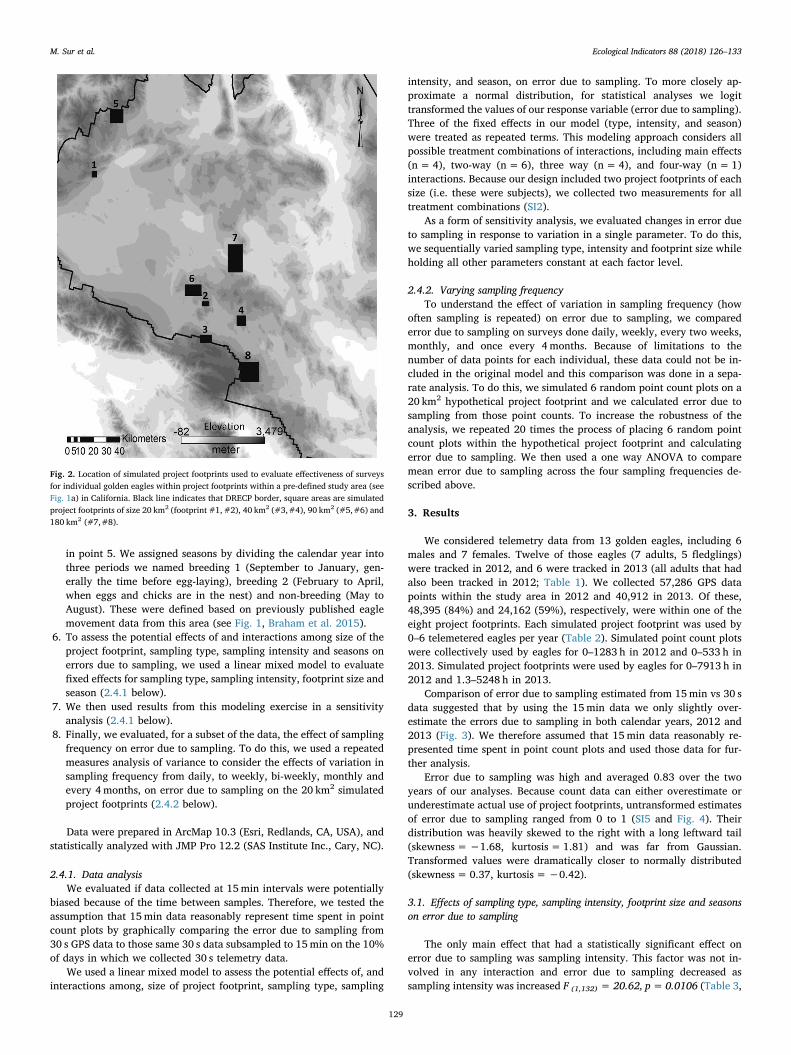
1. We simulated project footprints of 20, 40, 90 and 180 km2 to cap-ture a range of sizes of wind facilities (Fig. 2). A description of thesize, shape and placement of footprints in the study area are pro-vided in SI3. Information on number of birds and GPS fixes re-presented within each simulated project footprint is provided in theresults.

2. We simulated modified fixed-radius point count plots within thosefootprints according to different sampling strategies (SI4 and point 5below) and calculated the amount of time that telemetered eaglesspent in the point count plots and in the simulated footprints (SI2).

3. We compared the amount of time telemetered eagles spent in point

1 Further details on telemetry systems, their attachment to birds, the data they collect,

(footnote continued)post-processing of those data, and the interpretation of these data and their relevance toeagle biology are available elsewhere (Lanzone et al., 2012; Duerr et al., 2015; Milleret al., 2014; Braham et al., 2015; Katzner et al., 2015).

M. Sur et al. Ecological Indicators 88 (2018) 126–133

127

count plots to the time they spent in the simulated project footprintsand we evaluated the strength of the relationship between the twoi.e., the “error due to sampling”. To do this, we first calculated thepredicted time spent in project footprints using the formula:

⎜ ⎟= ⎛⎝

⎞⎠

∗actual

Predicted time spent in the project footprint

time spent in point count plotssampling intensity (%)

100(1)

We then used the actual time spent in the project footprint (mea-sured by GPS telemetry) to calculate the relative error in measure-ment (derived from Bowerman et al., 2004) or here, an “error due tosampling”, defined as follows:

=−

actual

predictedactual

error due to sampling

time spent in the project footprint

time spent in the project footprinttime spent in the project footprint

( )

( )

(2)

4. We did this for two years of data and 24 point count approachescomposed of all combinations of:a. three different point count sampling types (random, systematic,

stratified by altitude) (SI4),b. two different sampling intensities (30% or 60% area coverage)

(SI4),c. four different project footprint sizes (2 replicates each of: 20, 40,

90 and 180 km2) (SI3 and SI4);5. To account for seasonal changes in eagle biology and, thus, the

availability of eagles to be counted, we calculated error due tosampling by season for all combinations of the sampling approaches

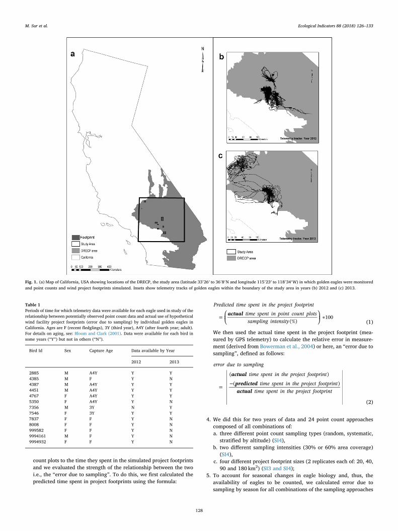
Fig. 1. (a) Map of California, USA showing locations of the DRECP, the study area (latitude 33°26′ to 36°8′N and longitude 115°23′ to 118°34′W) in which golden eagles were monitoredand point counts and wind project footprints simulated. Insets show telemetry tracks of golden eagles within the boundary of the study area in years (b) 2012 and (c) 2013.

Table 1Periods of time for which telemetry data were available for each eagle used in study of therelationship between potentially observed point count data and actual use of hypotheticalwind facility project footprints (error due to sampling) by individual golden eagles inCalifornia. Ages are F (recent fledglings), 3Y (third year), A4Y (after fourth year; adult).For details on aging, see: Bloom and Clark (2001). Data were available for each bird insome years (“Y”) but not in others (“N”).

Bird Id Sex Capture Age Data available by Year

2012 2013

2885 M A4Y Y Y4385 M F Y N4387 M A4Y Y Y4451 M A4Y Y Y4767 F A4Y Y Y5350 F A4Y Y N7356 M 3Y N Y7546 F 3Y Y Y7837 F F Y N8008 F F Y N999582 F F Y N9994161 M F Y N9994932 F F Y N

M. Sur et al. Ecological Indicators 88 (2018) 126–133

128

in point 5. We assigned seasons by dividing the calendar year intothree periods we named breeding 1 (September to January, gen-erally the time before egg-laying), breeding 2 (February to April,when eggs and chicks are in the nest) and non-breeding (May toAugust). These were defined based on previously published eaglemovement data from this area (see Fig. 1, Braham et al. 2015).

6. To assess the potential effects of and interactions among size of theproject footprint, sampling type, sampling intensity and seasons onerrors due to sampling, we used a linear mixed model to evaluatefixed effects for sampling type, sampling intensity, footprint size andseason (2.4.1 below).

7. We then used results from this modeling exercise in a sensitivityanalysis (2.4.1 below).

8. Finally, we evaluated, for a subset of the data, the effect of samplingfrequency on error due to sampling. To do this, we used a repeatedmeasures analysis of variance to consider the effects of variation insampling frequency from daily, to weekly, bi-weekly, monthly andevery 4months, on error due to sampling on the 20 km2 simulatedproject footprints (2.4.2 below).

Data were prepared in ArcMap 10.3 (Esri, Redlands, CA, USA), andstatistically analyzed with JMP Pro 12.2 (SAS Institute Inc., Cary, NC).

2.4.1. Data analysisWe evaluated if data collected at 15min intervals were potentially

biased because of the time between samples. Therefore, we tested theassumption that 15min data reasonably represent time spent in pointcount plots by graphically comparing the error due to sampling from30 s GPS data to those same 30 s data subsampled to 15min on the 10%of days in which we collected 30 s telemetry data.

We used a linear mixed model to assess the potential effects of, andinteractions among, size of project footprint, sampling type, sampling

intensity, and season, on error due to sampling. To more closely ap-proximate a normal distribution, for statistical analyses we logittransformed the values of our response variable (error due to sampling).Three of the fixed effects in our model (type, intensity, and season)were treated as repeated terms. This modeling approach considers allpossible treatment combinations of interactions, including main effects(n= 4), two-way (n= 6), three way (n=4), and four-way (n=1)interactions. Because our design included two project footprints of eachsize (i.e. these were subjects), we collected two measurements for alltreatment combinations (SI2).

As a form of sensitivity analysis, we evaluated changes in error dueto sampling in response to variation in a single parameter. To do this,we sequentially varied sampling type, intensity and footprint size whileholding all other parameters constant at each factor level.

2.4.2. Varying sampling frequencyTo understand the effect of variation in sampling frequency (how

often sampling is repeated) on error due to sampling, we comparederror due to sampling on surveys done daily, weekly, every two weeks,monthly, and once every 4months. Because of limitations to thenumber of data points for each individual, these data could not be in-cluded in the original model and this comparison was done in a sepa-rate analysis. To do this, we simulated 6 random point count plots on a20 km2 hypothetical project footprint and we calculated error due tosampling from those point counts. To increase the robustness of theanalysis, we repeated 20 times the process of placing 6 random pointcount plots within the hypothetical project footprint and calculatingerror due to sampling. We then used a one way ANOVA to comparemean error due to sampling across the four sampling frequencies de-scribed above.

3. Results

We considered telemetry data from 13 golden eagles, including 6males and 7 females. Twelve of those eagles (7 adults, 5 fledglings)were tracked in 2012, and 6 were tracked in 2013 (all adults that hadalso been tracked in 2012; Table 1). We collected 57,286 GPS datapoints within the study area in 2012 and 40,912 in 2013. Of these,48,395 (84%) and 24,162 (59%), respectively, were within one of theeight project footprints. Each simulated project footprint was used by0–6 telemetered eagles per year (Table 2). Simulated point count plotswere collectively used by eagles for 0–1283 h in 2012 and 0–533 h in2013. Simulated project footprints were used by eagles for 0–7913 h in2012 and 1.3–5248 h in 2013.

Comparison of error due to sampling estimated from 15min vs 30 sdata suggested that by using the 15min data we only slightly over-estimate the errors due to sampling in both calendar years, 2012 and2013 (Fig. 3). We therefore assumed that 15min data reasonably re-presented time spent in point count plots and used those data for fur-ther analysis.

Error due to sampling was high and averaged 0.83 over the twoyears of our analyses. Because count data can either overestimate orunderestimate actual use of project footprints, untransformed estimatesof error due to sampling ranged from 0 to 1 (SI5 and Fig. 4). Theirdistribution was heavily skewed to the right with a long leftward tail(skewness=−1.68, kurtosis= 1.81) and was far from Gaussian.Transformed values were dramatically closer to normally distributed(skewness= 0.37, kurtosis=−0.42).

3.1. Effects of sampling type, sampling intensity, footprint size and seasonson error due to sampling

The only main effect that had a statistically significant effect onerror due to sampling was sampling intensity. This factor was not in-volved in any interaction and error due to sampling decreased assampling intensity was increased F (1,132) = 20.62, p= 0.0106 (Table 3,

Fig. 2. Location of simulated project footprints used to evaluate effectiveness of surveysfor individual golden eagles within project footprints within a pre-defined study area (seeFig. 1a) in California. Black line indicates that DRECP border, square areas are simulatedproject footprints of size 20 km2 (footprint #1, #2), 40 km2 (#3,#4), 90 km2 (#5,#6) and180 km2 (#7,#8).

M. Sur et al. Ecological Indicators 88 (2018) 126–133

129

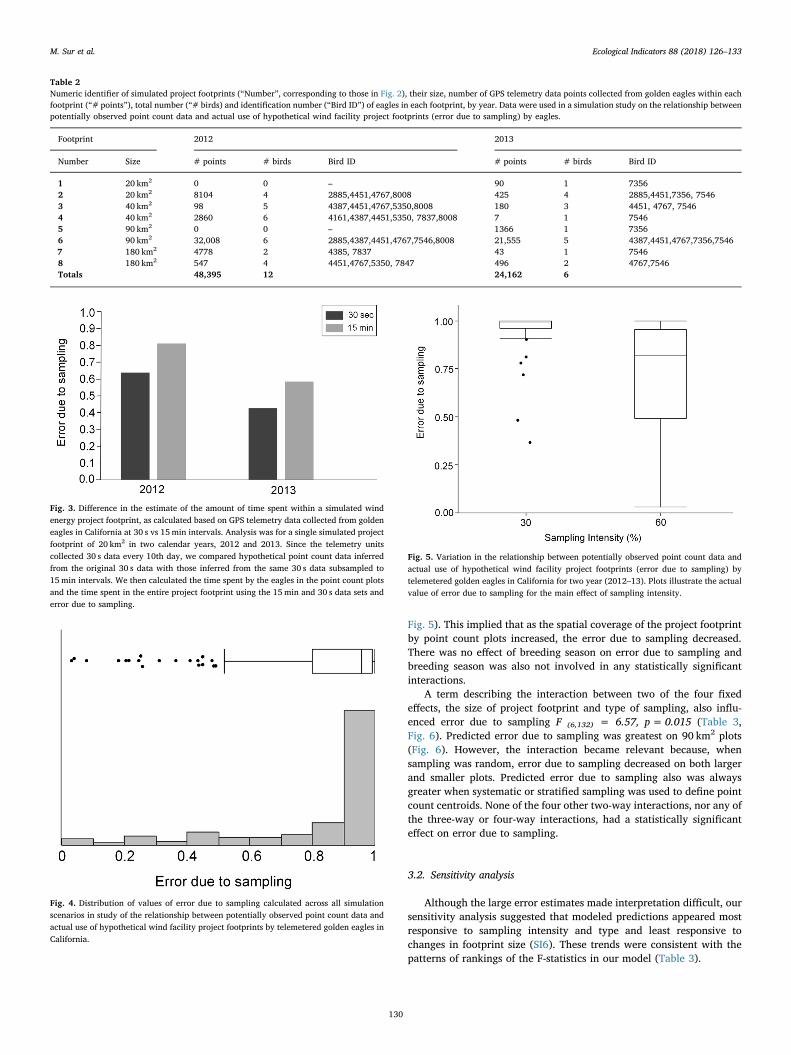
Fig. 5). This implied that as the spatial coverage of the project footprintby point count plots increased, the error due to sampling decreased.There was no effect of breeding season on error due to sampling andbreeding season was also not involved in any statistically significantinteractions.

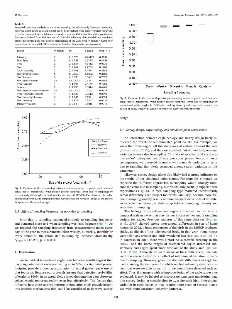
A term describing the interaction between two of the four fixedeffects, the size of project footprint and type of sampling, also influ-enced error due to sampling F (6,132) = 6.57, p= 0.015 (Table 3,Fig. 6). Predicted error due to sampling was greatest on 90 km2 plots(Fig. 6). However, the interaction became relevant because, whensampling was random, error due to sampling decreased on both largerand smaller plots. Predicted error due to sampling also was alwaysgreater when systematic or stratified sampling was used to define pointcount centroids. None of the four other two-way interactions, nor any ofthe three-way or four-way interactions, had a statistically significanteffect on error due to sampling.

3.2. Sensitivity analysis

Although the large error estimates made interpretation difficult, oursensitivity analysis suggested that modeled predictions appeared mostresponsive to sampling intensity and type and least responsive tochanges in footprint size (SI6). These trends were consistent with thepatterns of rankings of the F-statistics in our model (Table 3).

Table 2Numeric identifier of simulated project footprints (“Number”, corresponding to those in Fig. 2), their size, number of GPS telemetry data points collected from golden eagles within eachfootprint (“# points”), total number (“# birds) and identification number (“Bird ID”) of eagles in each footprint, by year. Data were used in a simulation study on the relationship betweenpotentially observed point count data and actual use of hypothetical wind facility project footprints (error due to sampling) by eagles.

Footprint 2012 2013

Number Size # points # birds Bird ID # points # birds Bird ID

1 20 km2 0 0 – 90 1 73562 20 km2 8104 4 2885,4451,4767,8008 425 4 2885,4451,7356, 75463 40 km2 98 5 4387,4451,4767,5350,8008 180 3 4451, 4767, 75464 40 km2 2860 6 4161,4387,4451,5350, 7837,8008 7 1 75465 90 km2 0 0 – 1366 1 73566 90 km2 32,008 6 2885,4387,4451,4767,7546,8008 21,555 5 4387,4451,4767,7356,75467 180 km2 4778 2 4385, 7837 43 1 75468 180 km2 547 4 4451,4767,5350, 7847 496 2 4767,7546Totals 48,395 12 24,162 6

Fig. 3. Difference in the estimate of the amount of time spent within a simulated windenergy project footprint, as calculated based on GPS telemetry data collected from goldeneagles in California at 30 s vs 15min intervals. Analysis was for a single simulated projectfootprint of 20 km2 in two calendar years, 2012 and 2013. Since the telemetry unitscollected 30 s data every 10th day, we compared hypothetical point count data inferredfrom the original 30 s data with those inferred from the same 30 s data subsampled to15min intervals. We then calculated the time spent by the eagles in the point count plotsand the time spent in the entire project footprint using the 15min and 30 s data sets anderror due to sampling.

Fig. 4. Distribution of values of error due to sampling calculated across all simulationscenarios in study of the relationship between potentially observed point count data andactual use of hypothetical wind facility project footprints by telemetered golden eagles inCalifornia.

Fig. 5. Variation in the relationship between potentially observed point count data andactual use of hypothetical wind facility project footprints (error due to sampling) bytelemetered golden eagles in California for two year (2012–13). Plots illustrate the actualvalue of error due to sampling for the main effect of sampling intensity.

M. Sur et al. Ecological Indicators 88 (2018) 126–133

130

3.3. Effect of sampling frequency on error due to sampling

Error due to sampling responded strongly to sampling frequencyand plateaued close to 1 when sampling was least frequent (Fig. 7). Aswe reduced the sampling frequency from measurements taken everyday of the year to measurements taken weekly, bi-weekly, monthly orevery 4months, the errors due to sampling increased dramaticallyF(4,95)= 113.296, p < 0.001.

4. Discussion

For individual telemetered eagles, our best-case results suggest thatday-long point count surveys covering up to 60% of a simulated projectfootprint provide a poor approximation of actual golden eagle use ofthat footprint. Because our protocols assume that detection probabilityof eagles is 100%, in an actual field survey the sampling data observerscollect would represent reality even less effectively. The factors thatinfluence how these surveys perform in simulation trials provide insightinto specific mechanisms that could be considered to improve survey

design.

4.1. Survey design, eagle ecology and simulated point count results

An interaction between eagle ecology and survey design likely in-fluenced the results of our simulated point counts. For example, weknew that these eagles left the study area at certain times of the year(Braham et al., 2015), and thus we expected, but did not find, seasonalvariation in error due to sampling. This lack of an effect is likely due tothe eagles’ infrequent use of any particular project footprint. As aconsequence, we observed dramatic within-month variation in errordue to sampling that likely swamped among-season variation in thisparameter.

Likewise, survey design alone also likely had a strong influence onthe results of our simulated point counts. For example, although weexpected that different approaches to sampling would strongly influ-ence the error due to sampling, our results only partially support theseexpectations (Fig. 6). In fact, sampling type mattered inconsistentlyacross differently sized project footprints. Similarly, because more fre-quent sampling usually results in more frequent detections of wildlife,we expected, and found, a relationship between sampling intensity anderror due to sampling.

The biology of the telemetered eagles influenced our results at atemporal scale in a way that may further inform refinement of samplingdesigns for eagles. Previous analyses of this same data set (Brahamet al., 2015) showed strong inter-annual differences in size of homeranges. In 2012, a large proportion of the birds in the DRECP producedchicks, as did six of our telemetered birds. In that year, home rangeswere relatively smaller and birds wandered less (Braham et al., 2015).In contrast, in 2013 there was almost no successful breeding in theDRECP and the home ranges of telemetered eagles increased sub-stantially and eagles spent more time out of the study area (Brahamet al., 2015). Although we were aware of these differences, our datawere too sparse to test for an effect of inter-annual variation in errordue to sampling. However, given the dramatic differences in eagle be-havior among the two years for which we had telemetry data, we sus-pect that were we able to test for it, we would have detected such aneffect. Thus, if managers wish to improve design of the eagle surveys weevaluated, it may be helpful to incorporate long-term monitoring datainto survey design at specific sites (e.g., a site with high inter-annualvariation in eagle behavior may require more years of surveys than asite with more consistent behavior patterns).

Table 3Repeated measures analysis of variance assessing the relationship between potentiallyobserved point count data and actual use of hypothetical wind facility project footprints(error due to sampling) by telemetered golden eagles in California. Simulated point countdata were derived from GIS analysis of GPS-GSM telemetry data overlaid on simulatedproject footprints. Bold font denotes significance at the 0.05 level. # param=number ofparameters in the model, DF= degrees of freedom (numerator, denominator).

Factor # param DF F Ratio Prob > F

Intensity 1 1, 3.978 20.6173 0.0106Size*Type 6 6, 6.551 6.5775 0.0151Type 2 2, 6.664 4.1412 0.0678Size 3 3, 4.061 2.7252 0.1768Type*Intensity 2 2, 7.308 1.7553 0.2385Size*Type*Intensity 6 6, 7.159 1.6202 0.2682Size*Seasons 6 6, 6.933 0.5431 0.7627Size*Type*Seasons 12 12, 13.93 0.5337 0.8588Type*Seasons 4 4, 14.04 0.4149 0.7952Seasons 2 2, 7.036 0.3814 0.6962Size*Type*Intensity*Seasons 12 12, 14.23 0.3722 0.9534Type*Intensity*Seasons 4 4, 14.39 0.3512 0.8390Size*Intensity*Seasons 6 6, 7.045 0.152 0.9824Size*Intensity 3 3, 3.879 0.1507 0.9239Intensity*Seasons 2 2, 7.14 0.1015 0.9048

Fig. 6. Variation in the relationship between potentially observed point count data andactual use of hypothetical wind facility project footprints (error due to sampling) bytelemetered golden eagles in California for two years (2012–13). Plots illustrate the valueof predicted error due to sampling for two-way interactions between (a) size of the projectfootprint and (b) sampling type.

Fig. 7. Variation in the relationship between potentially observed point count data andactual use of hypothetical wind facility project footprints (error due to sampling) bytelemetered golden eagles in California resulting from hypothetical point counts con-ducted at daily, weekly, bi-weekly, monthly or every 4months intervals.

M. Sur et al. Ecological Indicators 88 (2018) 126–133

131

Finally, in evaluating survey design, it is important to bear in mindthat most of our calculations were based on best case scenarios in whichsurveys were conducted continuously throughout the year. It is there-fore intuitive that as we reduced our sampling frequency to more rea-listic scenarios of weekly, monthly or every 4months, the efficacy of thepoint counts declined significantly. Continuous monitoring is rarelypossible and monitoring regimes capable of detecting trends are wea-kened by observational and economic constraints (Field et al., 2005). Assuch, the patterns we observed are likely illustrative of the difficulty indesigning logistically feasible yet effective surveys for this species.

4.2. Improving point count sampling

Our statistical analyses suggest that efforts to improve eagle surveyscould focus especially on sampling frequency, sampling intensity, andaccounting for size of the project footprint. These factors were all re-flective of the number of observations of eagles collected. Taken to-gether they suggest that current surveys on point count plots may col-lect too few measurements to allow strong inference to projectfootprints.

For rare and sparsely-distributed species such as golden eagles,success in monitoring requires sampling designs that account for con-text-specific parameters such as the size and topography of the projectfootprint. It has been suggested that the number of point count surveysshould factor in the size of the project and representative habitats atturbines (Strickland et al., 2011). An innovative approach to solvingthis sampling problem may be use of resource selection functions (RSF;Manly et al., 2002a) to design a stratified sampling scheme (Thompson,2004). This technique involves creating a RSF to describe the likelihoodof use of each habitat type present and then stratifying sampling tofocus on habitat types that the focal species is selecting. Often thisprocess requires a two-phase approach, with an initial survey to esti-mate resource selection functions that can be used in phase two to as-sign survey plot locations (Manly et al., 2002b)

The variation we observed in error due to sampling speaks to theneed to adjust sampling to account for local eagle ecology. For example,golden eagles can show many types of seasonal movements (Watson,2010; Watson et al., 2014; Braham et al., 2015). Although an eagle inCalifornia desert may spend all year tightly on a territory, eaglescounted there may include seasonal migrants to the region and localeagles may show altitudinal or short-distance seasonal movements thatinfluence detection rates. Adaptive sampling designs have been used toimprove precision and efficiency of surveys to aid management out-comes (Thompson, 1990; Yoccoz et al., 2001). Adapting surveys foreagles to account for these movements would likely reduce error due tosampling and improve the information surveys provide.

5. Conclusions

Improving wildlife surveys to avoid or minimize potential con-sequences of energy infrastructure development on species can bechallenging, expensive and time-consuming. Simulations can be an ef-fective way to test the efficiency of candidate survey methods. Althoughour work focuses on individual eagles (not eagle populations), ouranalysis shows the utility of simulations as a potential mechanism toimprove surveys at wind energy facilities by considering the context-specific way point counts are laid out on the landscape. Our work de-monstrates not only the problems associated with sampling for speciessuch as golden eagles, but also that the effectiveness of point countsampling at wind facilities is strongly dependent on the size of the windfacilities, the type of sampling undertaken and the degree to whichpoint count plots cover the area of the project footprint. Continuedevaluation and improvement of monitoring efforts could proceed fur-ther using empirical data, incorporating meteorological and topo-graphic information to better understand eagle flight, or running si-mulations in an iterative framework such as we present here. Such

future efforts should also explore how these results, based on samplingof individuals, relate to use of the project footprint by eagle populationsmore broadly.

Acknowledgments

Telemetry data collection was funded by Bureau of LandManagement grant agreement L11PX02237; this analysis of those datawas supported by U.S. Fish and Wildlife Service through an inter-agency agreement with the U.S. Geological Survey (#4500069170).Statement of author contributions: the USFWS Eagle TechnicalAssessment Team developed the concept for this study, all authorscontributed to study design, MS, TK and JB designed the statisticalanalyses and MS and JB carried out those analyses, MS and TK ledwriting of the manuscript, all authors revised the manuscript. Any useof trade, product, or firm names is for descriptive purposes only anddoes not imply endorsement by the U.S. Government. The findings andconclusions in this article are those of the authors and do not ne-cessarily represent the views of the U.S. Fish and Wildlife Service.

Appendix A. Supplementary data

Supplementary data associated with this article can be found, in theonline version, at http://dx.doi.org/10.1016/j.ecolind.2018.01.024.

References

Arnett, E.B., Brown, W.K., Erickson, W.P., Fiedler, J.K., Hamilton, B.L., Henry, T.H., Jain,A., Johnson, G.D., Kerns, J., Koford, R.R., Nicholson, C.P., O’Connell, T.J.,Piorkowski, M.D., Tankersley, R.D., 2008. Patterns of bat fatalities at wind energyfacilities in North America. J. Wildl. Manage. 72, 61–78.

Bloom, P.H., Clark, W.S., 2001. Molt and sequence of plumages of golden eagles and atechnique for inhand ageing. N. Am. Bird Bander 26, 97–116.

Bowerman, B., O’Connell, R., Koehler, A., 2004. Forecasting: Methods and Applications.Thompson Brooks/Cole, Belmont, CA.

Braham, M., Miller, T., Duerr, A.E., Lanzone, M., Fesnock, A., LaPre, L., Driscoll, D.,Katzner, T., 2015. Home in the heat: dramatic seasonal variation in home range ofdesert golden eagles informs management for renewable energy development. Biol.Conserv. 186, 225–232.

De Lucas, M., Janss, G.F.E., Whitfield, D.P., Ferrer, M., 2008. Collision fatality of raptorsin wind farms does not depend on raptor abundance. J. Appl. Ecol. 45, 1695–1703.

Douglas, D.J., Follestad, A., Langston, R.H., Pearce-Higgins, J.W., 2012. Modelled sen-sitivity of avian collision rate at wind turbines varies with number of hours of flightactivity input data. Ibis 154, 858–861.

Draft Desert Renewable Energy Conservation Plan and EIR/EIS, 2014. Renewable EnergyAction Team, CA, USA.

Drewitt, A.L., Langston, R.H., 2006. Assessing the impacts of wind farms on birds. Ibis148, 29–42.

Duerr, A.E., Miller, T.A., Lanzone, M., Brandes, D., Cooper, J., O'Malley, K., Katzner, T.,2015. Flight response of slope-soaring birds to seasonal variation in thermal gen-eration. Funct. Ecol. 29, 779–790.

Field, S.A., Tyre, A.J., Possingham, H.P., 2005. Optimizing allocation of monitoring effortunder economic and observational constraints. J. Wildl. Manage. 69, 473–482.

Fuller, M.R., Mosher, J.A., 1981. Methods of detecting and counting raptors: a review.Stud. Avian Biol. 6, 264.

Garman, S.L., Schweiger, E.W., Manier, D.J., 2012. Simulating future uncertainty to guidethe selection of survey designs for long-term monitoring. In: Gitzen, R.A., Millspaugh,J.J., Cooper, A.B., Licht, D.S. (Eds.), Design and Analysis of Long-term EcologicalMonitoring Studies. Camibridge University Press, pp. 228–250.

Gibbs, J.P., Snell, H.L., Causton, C.E., 2013. Wildlife for adaptive effective monitoring:lessons from the Galapagos Islands management. J. Wildl. Manage. 63, 1055–1065.

Hunt, G., 2002. Golden Eagles in a Perilous Landscape: Predicting the Effects ofMitigation for Wind Turbine Blade-Strike Mortality. California Energy CommissionConsultant Report.

Katzner, T.E., Brandes, D., Miller, T., Lanzone, M., Maisonneuve, C., Tremblay, J.A.,Mulvihill, R., Merovich, G.T., 2012. Topography drives migratory flight altitude ofgolden eagles: implications for on-shore wind energy development. J. Appl. Ecol. 49,1178–1186.

Katzner, T.E., Turk, P.J., Duerr, A.E., Miller, T.A., Lanzone, M.J., Cooper, J.L., Lemaître,J., 2015. Use of multiple modes of flight subsidy by a soaring terrestrial bird, thegolden eagle Aquila chrysaetos, when on migration. J. R. Soc. Interface 12,20150530.

Kenward, R.E., 1985. Raptor radio-tracking and telemetry. ICBP Tech. Publ. 5, 409–420.Kiesecker, J.M., Evans, J.S., Fargione, J., Doherty, K., Foresman, K.R., Kunz, T.H., Naugle,

D., Nibbelink, N.P., Niemuth, N.D., 2011. Win-win for wind and wildlife: a vision tofacilitate sustainable development. PLoS One 6, 1–8.

Kunz, T.H., Arnett, E.B., Erickson, W.P., Hoar, A.R., Johnson, G.D., Larkin, R.P.,

M. Sur et al. Ecological Indicators 88 (2018) 126–133

132

Strickland, M.D., Thresher, R.W., Tuttle, M.D., 2007. Ecological impacts of windenergy development on bats: questions, research needs, and hypotheses. Front. Ecol.Environ. 5, 315–324.

Lanzone, M.J., Miller, T.A., Turk, P., Brandes, D., Halverson, C., Maisonneuve, C.,Tremblay, J., Cooper, J., O'Malley, K., Brooks, R.P., Katzner, T., 2012. Flight re-sponses by a migratory soaring raptor to changing meteorological conditions. Biol.Lett. 8, 710–713.

Latta, B., Thelander, C., 2013. Results of 2012 Golden Eagle Nesting Surveys of theCalifornia Desert and Northern California Districts. Final Rep. BioResourceConsultants Inc., Ojai, CA.

Manly, B.F., McDonald, L., Thomas, D., McDonald, T., Erickson, W., 2002a. ResourceSelection by Animals: Statistical Design and Analysis for Field Studies, Second edi-tion. Kluwer Press, New York, New York, USA.

Manly, B.F., Akroyd, J.A.M., Walshe, K.A., 2002b. Two-phase stratified random surveyson multiple populations at multiple locations. N. Z. J. Mar. Freshwater Res. 36,581–591.

Miller, T.A., Brooks, R.P., Lanzone, M., Brandes, D., Cooper, J., O’Malley, K.,Maisonneuve, C., Tremblay, J., Duerr, A., Katzner, T., 2014. Assessing risk to birdsfrom industrial wind energy development via paired resource selection models.Conserv. Biol. 28, 745–755.

New, L., Bjerre, E., Millsap, B., Otto, M.C., Runge, M.C., 2015. A collision risk model topredict avian fatalities at wind facilities: an example using Golden Eagle, Aquilachrysaetos. PloS One 10, e0130978.

Pruett, C.L., Patten, M.A., Wolfe, D.H., 2009. It’s not easy being green: wind energy and adeclining grassland bird. Bioscience 59, 257–262.

Ralph, C.J., Sauer, J.R., Droege, S., 1995. Monitoring Bird Populations by Point Counts.Gen. Tech. Rep. PSW-GTR-149. U.S. Department of Agriculture, Forest Service,Pacific Southwest Research Station, Albany, CA, pp. 187.

Soanes, L.M., Arnould, J.P., Dodd, S.G., Sumner, M.D., Green, J.A., 2013. How manyseabirds do we need to track to define home-range area? J. Appl. Ecol. 50, 671–679.

Strickland, M.D., Arnett, E.B., Erickson, W.P., Johnson, D.H., Johnson, G.D., Morrison,M.L., Shaffer, J.A., Warren-Hicks, W., 2011. Comprehensive Guide to Studying WindEnergy/Wildlife Interactions. Prepared for the National Wind CoordinatingCollaborative, Washington, D.C., USA.

Thompson, S.K., 1990. Adaptive cluster sampling. J. Am. Stat. Assoc. 85, 1050–1059.Thompson, W., 2004. Sampling Rare or Elusive Species: Concepts, Designs, and

Techniques for Estimating Population Parameters. Island Press, Washington, DC.USFWS, 2013. Eagle Conservation Plan Guidance Module 1 – Land-Based Wind Energy.

Version 2. U.S. Fish and Wildlife Service.Watson, J., 2010. The Golden Eagle, Second edition. T&AD Poyser, London.Watson, J.W., Duff, A.A., Davies, R.W., 2014. Home range and resource selection by gps-

monitored adult golden eagles in the Columbia plateau ecoregion: implications forwind power development. J. Wildl. Manage. 78, 1012–1021.

Yoccoz, N.G., Nichols, J.D., Boulinier, T., 2001. Monitoring of biological diversity inspace and time. Trends Ecol. Evol. 16, 446–453.

M. Sur et al. Ecological Indicators 88 (2018) 126–133

133

SI1: The US Fish and Wildlife Eagle Conservation Plan Guidance (ECPG) provides specific

recommendations for point count surveys of golden eagles to assess use of existing and proposed

wind facilities (e.g. Strickland et al. 2011, USFWS 2013). These can be summarized as follows:

point counts carried out from the center of a fixed 800 m radius plot (~2 km2);

plots located either randomly, systematically or in a stratified manner within the

project footprint (we refer to these as “sampling types”);

point count centroids at vantage points to maximize visibility of eagles;

plots laid out such that there is ≥30% spatial coverage of the project footprint (we

refer to spatial coverage as the “sampling intensity”);

recording the number of eagles observed and the number of minutes they were in

flight within the plot;

conducting point counts for 1, 2 or more hrs.

Beyond ensuring a minimum of 30% coverage of a facility, the Eagle Conservation Plan makes

only general recommendations about adjusting sampling effort based on the size of the wind

facility.

SI2: Converting telemetry data to hypothetical survey data.

To convert our telemetry data to hypothetical survey data, we simulated modified point count

plots within project footprints. Locations for point count stations were selected based on the

different sampling approaches (SI3). We then used telemetry data from the 13 instrumented

golden eagles to calculate the time spent by each bird in 800m plots centered on those stations.

These data differ from those collected during a true eagle point count because a true count would

include observations from all eagles detected, regardless of whether or not they were

telemetered. Our data only include observations from our telemetered birds and other non-

telemetered eagles may have been present at the same time.

We assumed that birds entered the sampling plot at the time of the first fix located within the plot

and that they left at the time of the first subsequent fix located outside the plot; that is, we did not

try to interpolate time or distance between points. Because we used GPS fixes as a proxy for

human observations, our analysis also simplifies the reality of sampling by assuming that all

possible observations of individual animals are recorded and that detection probability is 100%.

We calculated the total time spent by the birds in the point count plots and the time spent in the

project footprint as if a counter was present all day every day, all year (i.e., conducting

continuous surveys). We assume that estimates of error due to sampling generated by continuous

sampling are best-case scenarios as compared to shorter surveys that would normally be

conducted during point count sampling.

SI3: Details of size, shape and placement of simulated wind facility project footprints used to

evaluate effectiveness of surveys for individual golden eagles within a pre-defined study area

(see Fig. 1a) in California.

We simulated project footprints of 20, 40, 90 and 180 km2 to capture a range of sizes of wind

facilities (Fig. 2). There were no consistent patterns that we could find in the shape of existing

project footprints and so we simulated only rectangular project footprints. This simplified our

analyses by assuming that estimation of eagle use of an area would not be influenced by the

shape of the project footprint.

We randomly selected potential locations for placement of the footprints within our study area.

We retained potential footprints if they contained >50 GPS telemetry fixes from eagles for at

least one of the two years of the study. If the potential footprint contained ≤50 fixes, we

discarded that location and we randomly selected a new location for the project footprint. We

iteratively repeated this process until all footprints were assigned non-overlapping positions on

the landscape (Fig. 2).

SI4: Details of factors used in the multifactorial analysis of variance to assess the potential 1

effects of and interactions among size of the project footprint, sampling type, sampling intensity 2

and seasons on errors due to sampling. 3

Sampling types 4

The ways in which point count plots are distributed within the simulated project footprints are 5

defined by the sampling type, which could be either simple random, systematic or stratified. In 6

all cases, the number of point count centroids was determined by the sampling intensity (below) 7

and the point count plots never overlapped. 8

Randomly located point count centroids were placed randomly within the project footprint. 9

Systematically located point count centroids were placed at the center of equally sized 10

rectangular grid cells whose number was determined by the sampling intensity. Stratified point 11

count centroids were placed randomly within the highest 40% of elevations in the plot, as 12

defined by a 30 m Digital Elevation Model (GMTED2010, Danielson and Gesch 2011). 13

Sampling intensity 14

The degree to which point count plots cover the area of the project footprint is defined by the 15

sampling intensity. We simulated two different sampling intensities, 30% (that suggested as a 16

minimum by USFWS) and 60%. To cover 30% of an area of a project footprint of size 20 km2, 17

the total area covered by point count plots would be 6 km2. Thus, a 20 km2 project footprint 18

requires three 2-km2 point count plots for 30% coverage and six plots for 60% coverage. 19

Size of project footprint 20

We defined four different project footprint sizes (20, 40, 90 and 180 km2), as described in SI2. 21

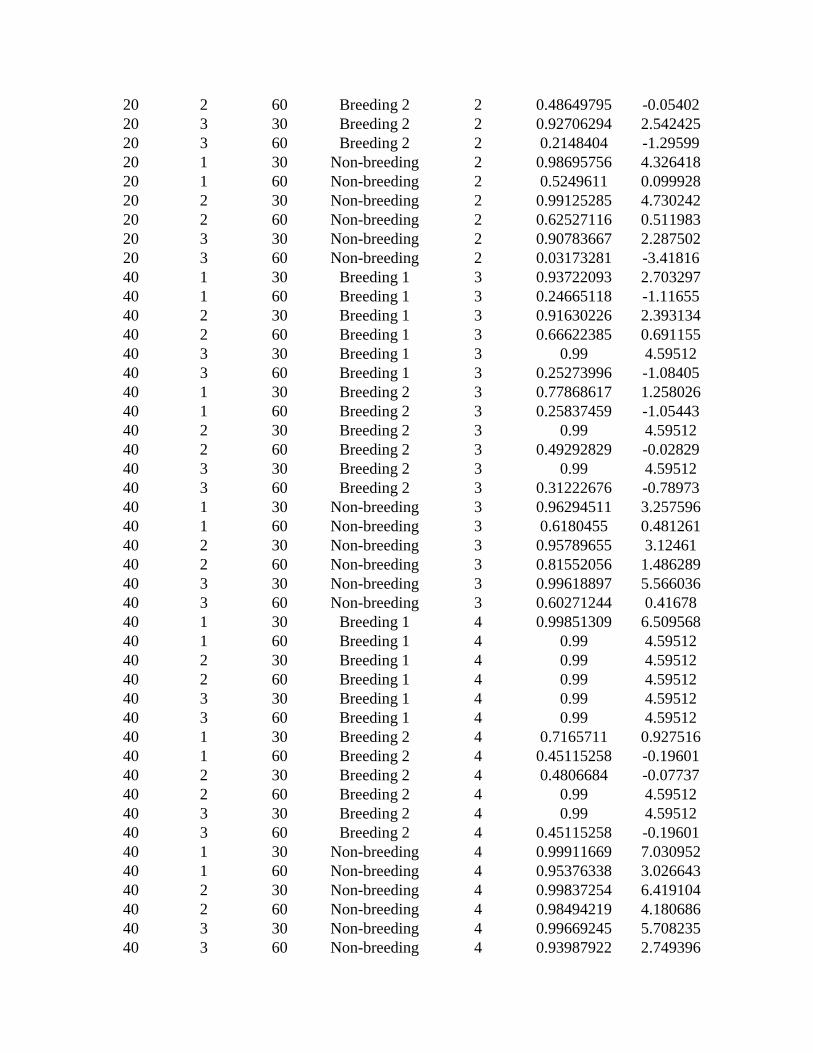
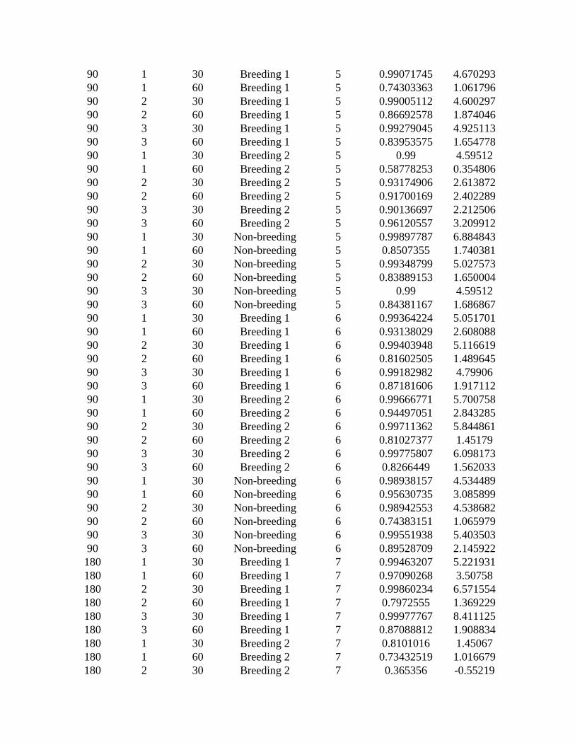
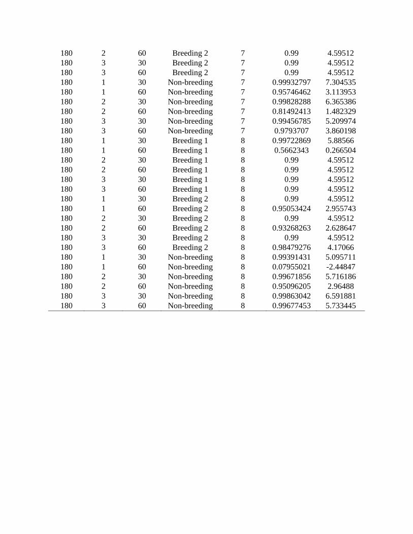
SI5: Raw data used in study of the relationship between potentially observed point count data 22

and actual use of hypothetical wind facility project footprints (error due to sampling) by 23

telemetered golden eagles in California. Data include error due to sampling and logit transformed 24

valued of error due to sampling for different sampling strategies due to variations in size of the 25

project footprint, sampling type, sampling intensity and seasons. Because our design included 26

two project footprints of each size (i.e. these were subjects), we collected two measurements for 27

all treatment combinations. 28

Size of

project

footprint

Sampling

Type

Sampling

Intensity Seasons Subject

Error due to

sampling

Logit

transformed

error due to

sampling

20 1 30 Breeding 1 1 . .

20 1 60 Breeding 1 1 . .

20 2 30 Breeding 1 1 . .

20 2 60 Breeding 1 1 . .

20 3 30 Breeding 1 1 . .

20 3 60 Breeding 1 1 . .

20 1 30 Breeding 2 1 . .

20 1 60 Breeding 2 1 . .

20 2 30 Breeding 2 1 . .

20 2 60 Breeding 2 1 . .

20 3 30 Breeding 2 1 . .

20 3 60 Breeding 2 1 . .

20 1 30 Non-breeding 1 0.91071806 2.322434

20 1 60 Non-breeding 1 0.518559 0.07427

20 2 30 Non-breeding 1 0.95039305 2.952745

20 2 60 Non-breeding 1 0.18193441 -1.5033

20 3 30 Non-breeding 1 0.93543128 2.673278

20 3 60 Non-breeding 1 0.2055228 -1.35213

20 1 30 Breeding 1 2 0.97797151 3.793144

20 1 60 Breeding 1 2 0.4108278 -0.36054

20 2 30 Breeding 1 2 0.9873891 4.360502

20 2 60 Breeding 1 2 0.43558968 -0.25908

20 3 30 Breeding 1 2 0.90873938 2.298339

20 3 60 Breeding 1 2 0.0397955 -3.18339

20 1 30 Breeding 2 2 0.96156124 3.219492

20 1 60 Breeding 2 2 0.4385707 -0.24696

20 2 30 Breeding 2 2 0.97554397 3.686118

20 2 60 Breeding 2 2 0.48649795 -0.05402

20 3 30 Breeding 2 2 0.92706294 2.542425

20 3 60 Breeding 2 2 0.2148404 -1.29599

20 1 30 Non-breeding 2 0.98695756 4.326418

20 1 60 Non-breeding 2 0.5249611 0.099928

20 2 30 Non-breeding 2 0.99125285 4.730242

20 2 60 Non-breeding 2 0.62527116 0.511983

20 3 30 Non-breeding 2 0.90783667 2.287502

20 3 60 Non-breeding 2 0.03173281 -3.41816

40 1 30 Breeding 1 3 0.93722093 2.703297

40 1 60 Breeding 1 3 0.24665118 -1.11655

40 2 30 Breeding 1 3 0.91630226 2.393134

40 2 60 Breeding 1 3 0.66622385 0.691155

40 3 30 Breeding 1 3 0.99 4.59512

40 3 60 Breeding 1 3 0.25273996 -1.08405

40 1 30 Breeding 2 3 0.77868617 1.258026

40 1 60 Breeding 2 3 0.25837459 -1.05443

40 2 30 Breeding 2 3 0.99 4.59512

40 2 60 Breeding 2 3 0.49292829 -0.02829

40 3 30 Breeding 2 3 0.99 4.59512

40 3 60 Breeding 2 3 0.31222676 -0.78973

40 1 30 Non-breeding 3 0.96294511 3.257596

40 1 60 Non-breeding 3 0.6180455 0.481261

40 2 30 Non-breeding 3 0.95789655 3.12461

40 2 60 Non-breeding 3 0.81552056 1.486289

40 3 30 Non-breeding 3 0.99618897 5.566036

40 3 60 Non-breeding 3 0.60271244 0.41678

40 1 30 Breeding 1 4 0.99851309 6.509568

40 1 60 Breeding 1 4 0.99 4.59512

40 2 30 Breeding 1 4 0.99 4.59512

40 2 60 Breeding 1 4 0.99 4.59512

40 3 30 Breeding 1 4 0.99 4.59512

40 3 60 Breeding 1 4 0.99 4.59512

40 1 30 Breeding 2 4 0.7165711 0.927516

40 1 60 Breeding 2 4 0.45115258 -0.19601

40 2 30 Breeding 2 4 0.4806684 -0.07737

40 2 60 Breeding 2 4 0.99 4.59512

40 3 30 Breeding 2 4 0.99 4.59512

40 3 60 Breeding 2 4 0.45115258 -0.19601

40 1 30 Non-breeding 4 0.99911669 7.030952

40 1 60 Non-breeding 4 0.95376338 3.026643

40 2 30 Non-breeding 4 0.99837254 6.419104

40 2 60 Non-breeding 4 0.98494219 4.180686

40 3 30 Non-breeding 4 0.99669245 5.708235

40 3 60 Non-breeding 4 0.93987922 2.749396

90 1 30 Breeding 1 5 0.99071745 4.670293

90 1 60 Breeding 1 5 0.74303363 1.061796

90 2 30 Breeding 1 5 0.99005112 4.600297

90 2 60 Breeding 1 5 0.86692578 1.874046

90 3 30 Breeding 1 5 0.99279045 4.925113

90 3 60 Breeding 1 5 0.83953575 1.654778

90 1 30 Breeding 2 5 0.99 4.59512

90 1 60 Breeding 2 5 0.58778253 0.354806

90 2 30 Breeding 2 5 0.93174906 2.613872

90 2 60 Breeding 2 5 0.91700169 2.402289

90 3 30 Breeding 2 5 0.90136697 2.212506

90 3 60 Breeding 2 5 0.96120557 3.209912

90 1 30 Non-breeding 5 0.99897787 6.884843

90 1 60 Non-breeding 5 0.8507355 1.740381

90 2 30 Non-breeding 5 0.99348799 5.027573

90 2 60 Non-breeding 5 0.83889153 1.650004

90 3 30 Non-breeding 5 0.99 4.59512

90 3 60 Non-breeding 5 0.84381167 1.686867

90 1 30 Breeding 1 6 0.99364224 5.051701

90 1 60 Breeding 1 6 0.93138029 2.608088

90 2 30 Breeding 1 6 0.99403948 5.116619

90 2 60 Breeding 1 6 0.81602505 1.489645

90 3 30 Breeding 1 6 0.99182982 4.79906

90 3 60 Breeding 1 6 0.87181606 1.917112

90 1 30 Breeding 2 6 0.99666771 5.700758

90 1 60 Breeding 2 6 0.94497051 2.843285

90 2 30 Breeding 2 6 0.99711362 5.844861

90 2 60 Breeding 2 6 0.81027377 1.45179

90 3 30 Breeding 2 6 0.99775807 6.098173

90 3 60 Breeding 2 6 0.8266449 1.562033

90 1 30 Non-breeding 6 0.98938157 4.534489

90 1 60 Non-breeding 6 0.95630735 3.085899

90 2 30 Non-breeding 6 0.98942553 4.538682

90 2 60 Non-breeding 6 0.74383151 1.065979

90 3 30 Non-breeding 6 0.99551938 5.403503

90 3 60 Non-breeding 6 0.89528709 2.145922

180 1 30 Breeding 1 7 0.99463207 5.221931

180 1 60 Breeding 1 7 0.97090268 3.50758

180 2 30 Breeding 1 7 0.99860234 6.571554

180 2 60 Breeding 1 7 0.7972555 1.369229

180 3 30 Breeding 1 7 0.99977767 8.411125

180 3 60 Breeding 1 7 0.87088812 1.908834

180 1 30 Breeding 2 7 0.8101016 1.45067

180 1 60 Breeding 2 7 0.73432519 1.016679

180 2 30 Breeding 2 7 0.365356 -0.55219

180 2 60 Breeding 2 7 0.99 4.59512

180 3 30 Breeding 2 7 0.99 4.59512

180 3 60 Breeding 2 7 0.99 4.59512

180 1 30 Non-breeding 7 0.99932797 7.304535

180 1 60 Non-breeding 7 0.95746462 3.113953

180 2 30 Non-breeding 7 0.99828288 6.365386

180 2 60 Non-breeding 7 0.81492413 1.482329

180 3 30 Non-breeding 7 0.99456785 5.209974

180 3 60 Non-breeding 7 0.9793707 3.860198

180 1 30 Breeding 1 8 0.99722869 5.88566

180 1 60 Breeding 1 8 0.5662343 0.266504

180 2 30 Breeding 1 8 0.99 4.59512

180 2 60 Breeding 1 8 0.99 4.59512

180 3 30 Breeding 1 8 0.99 4.59512

180 3 60 Breeding 1 8 0.99 4.59512

180 1 30 Breeding 2 8 0.99 4.59512

180 1 60 Breeding 2 8 0.95053424 2.955743

180 2 30 Breeding 2 8 0.99 4.59512

180 2 60 Breeding 2 8 0.93268263 2.628647

180 3 30 Breeding 2 8 0.99 4.59512

180 3 60 Breeding 2 8 0.98479276 4.17066

180 1 30 Non-breeding 8 0.99391431 5.095711

180 1 60 Non-breeding 8 0.07955021 -2.44847

180 2 30 Non-breeding 8 0.99671856 5.716186

180 2 60 Non-breeding 8 0.95096205 2.96488

180 3 30 Non-breeding 8 0.99863042 6.591881

180 3 60 Non-breeding 8 0.99677453 5.733445

-2

2

6

10

40 km2 footprint

20 40 90 180 1 2 3 30 60

a) Varying sampling intensity: Intensity = 30%

b) Varying sampling intensity: Intensity = 60%

Logit e

rror

Logit e

rror

Random sampling 30% sampling intensity

20 40 90 180 30 601 2 3

-2

2

6

10

40 km2 footprint Random sampling 60% sampling intensity

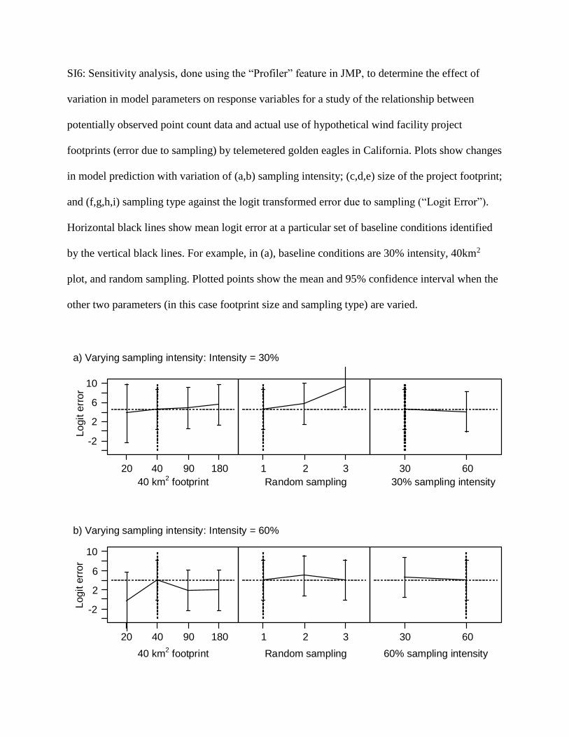
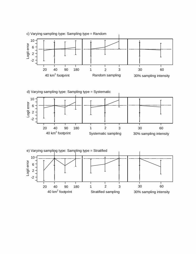
SI6: Sensitivity analysis, done using the “Profiler” feature in JMP, to determine the effect of

variation in model parameters on response variables for a study of the relationship between

potentially observed point count data and actual use of hypothetical wind facility project

footprints (error due to sampling) by telemetered golden eagles in California. Plots show changes

in model prediction with variation of (a,b) sampling intensity; (c,d,e) size of the project footprint;

and (f,g,h,i) sampling type against the logit transformed error due to sampling (“Logit Error”).

Horizontal black lines show mean logit error at a particular set of baseline conditions identified

by the vertical black lines. For example, in (a), baseline conditions are 30% intensity, 40km2

plot, and random sampling. Plotted points show the mean and 95% confidence interval when the

other two parameters (in this case footprint size and sampling type) are varied.

-2

2

6

10

20 40 90 180 1 2 3

Random sampling

30 60

-2

2

6

10

20 40 90 180 30 60

-2

2

6

10

20 40 90 180 30 60

c) Varying sampling type: Sampling type = Random

d) Varying sampling type: Sampling type = Systematic

e) Varying sampling type: Sampling type = Stratified

40 km2 footprint Systematic sampling 30% sampling intensity

Stratified sampling

1

1

2

2

3

3

Logit e

rror

Logit e

rror

Logit e

rror

40 km2 footprint 30% sampling intensity

40 km2 footprint 30% sampling intensity

-2

2

6

10

20 40 90 180 1 2 3 30 60

-2

2

6

10

20 40 90 180 30 60

-2

2

6

10

20 40 90 180 30 60

-2

2

6

10

20 40 90 180 30 60

f) Varying size of the project footprint: Size = 20km2

i) Varying size of the project footprint: Size = 180km2

h) Varying size of the project footprint: Size = 90km2

g) Varying size of the project footprint: Size = 40km2

1 2 3

1 2 3

1 2 3

Logit E

rror

Logit E

rror

Logit E

rror

Logit E

rror

Random sampling 30% sampling intensity20 km2 footprint

40 km2 footprint Random sampling 30% sampling intensity

90 km2 footprint Random sampling 30% sampling intensity

180 km2 footprint Random sampling 30% sampling intensity