The validation of machine-learning models for the stress

© Henry Stewart Publications 1752-8887 (2018) Vol. 11, 3 1–26 Journal of Risk Management in Financial Institutions 1

The validation of machine-learning models for the stress testing of credit riskReceived: 21st May, 2018

Michael Jacobs, Jris a Senior Vice-President at PNC Bank. He is a quantitative practitioner and researcher in the field of risk modelling and management. Prior to this, he was Principal Director at Accenture Consulting, Finance & Risk Advisory’s financial institutions, risk, regulatory and analytics practice. He has also worked as a senior economist with the US Office of the Comptroller of the Currency, a lead expert in enterprise and credit risk, and at J.P. Morgan Chase, where as a senior vice-president he led the empirical research and credit risk capital groups within the Risk Methodology Services division. He holds a doctorate in finance from the City University of New York, and is a Chartered Financial Analyst.

PNC Bank, APM Model Development, 340 Madison Avenue, New York, NY 10017, USA Tel: +1 917 324 2098; E-mail: [email protected]

Abstract Banking supervisors need to know the amount of capital resources required by an institution to support the risks taken. Traditional approaches, such as regulatory capital ratios, have proven inadequate, giving rise to stress-testing as a primary tool. The macroeconomic variables that supervisors provide to institutions for exercises such as the Comprehensive Capital Analysis and Review (CCAR) programme represent a critical input into this. A common approach to segment-level modelling is statistical regression, like vector autoregression (VAR), to exploit the dependency structure between macroeconomic drivers and modelling segments. However, linear models such as VAR are unable to model distributions that deviate from normality. This paper proposes a challenger approach in the machine-learning class of models, widely used in the academic literature, but not commonly employed in practice: the multivariate adaptive regression splines (MARS) model. The study empirically tests these models using Fed Y-9 filings and macroeconomic data, released by the regulators for CCAR purposes. The champion MARS model is validated through a rigorous comparison against the VAR model, and is found to exhibit greater accuracy and superior out-of-sample performance, according to various metrics across all modelling segments. The MARS model also produces more reasonable forecasts according to quality and conservatism.

Keywords: stress testing, CCAR, DFAST, credit risk, financial crisis, model risk, vector autoregression, multivariate adaptive regression splines, model validation

INTRODUCTIONIn the aftermath of the recent financial crisis,1,2 regulators have utilised stress testing as a means by which to evaluate the soundness of financial institutions’ risk management procedures. The primary means of risk management, particularly in the field of credit,3 is through advanced mathematical, statistical and quantitative techniques

and models, which leads to model risk. Model risk can be defined as the potential that a model does not sufficiently capture the risks it is used to assess, and the danger that it may underestimate potential risks in the future.4 Stress testing has been used by supervisors to assess the reliability of credit risk models, as can be seen in the revised Basel Framework5–15 and the Federal Reserve’s

RMFI0112_JACOBS_11-3.indd 1 13/06/18 6:35 PM

Jacobs, Jr.

2 Journal of Risk Management in Financial Institutions Vol. 11, 3 1–26 © Henry Stewart Publications 1752-8887 (2018)

Comprehensive Capital Analysis and Review (CCAR) programme.

Prior to the financial crisis, most of the most prominent financial institutions to fail (eg Lehman, Bear Stearns, Washington Mutual, Freddie Mac and Fannie Mae) were considered to be well capitalised according to the standards across a wide span of regulators. Another commonality among the large failed firms was a general exposure to residential real estate, either directly or through securitisation. Further, it is widely believed that the internal risk models of these institutions were not wildly out of line with those of the regulators.16 These unanticipated failures demonstrate that the answer to the question of how much capital an institution needs to avoid failure was not satisfactory. While capital models accept a non-zero probability of default according to the risk aversion of the institution or the supervisor, the utter failure of these constructs to even come close to projecting the perils that these institutions faced was a great motivator for considering alternative tools to assess capital adequacy, such as the stress-testing discipline.

Bank holding companies (BHCs) face a number of considerations in modelling losses for wholesale and retail lending portfolios. CCAR participants face some particular challenges in estimating losses based on scenarios and their associated risk drivers. The selection of modelling methodology must satisfy a number of criteria, such as suitability for portfolio type, materiality, data availability as well as alignment with chosen risk drivers. There are two broad categories of model types in use. Bottom-up models are loan or obligor-level models used by banks to forecast the expected losses of retail and wholesale loans for each loan. The expected loss is calculated for each loan, and then the sum of expected losses across all loans provides an estimate of portfolio losses, through conditioning on macroeconomic or financial/obligor specific variables. The primary advantages of bottom-up models are the ease of modelling the heterogeneity of underlying loans and the interaction of loan-level risk factors. The primary disadvantages of loan-level models are that while various loan-level methodologies can be used, these models are much more complex to specify and estimate. These models generally require more sophisticated econometric and simulation

techniques, and model validation standards may be more stringent. In contrast, top-down models are pool (or segment)-level models used by banks to forecast charge-off rates by retail and wholesale loan types as a function of macroeconomic and financial variables. In most cases for these models, banks use only one to four macroeconomic and financial risk drivers as explanatory variables. These variables are usually determined by interaction between model development teams and line-of-business experts. The primary advantage of top-down models has been the ready availability of data and the simplicity of model estimation. The primary disadvantage of pool-level models is that borrower-specific characteristics are generally not used as variables, except at the aggregate level using pool averages. Modelling challenges include determination of appropriate loss horizon (eg for CCAR it is a nine-quarter duration), determination of an appropriate averaging methodology, appropriate data segmentation and loss aggregation, as well as the annualisation of loss rates.

This section concludes by highlighting the key limitations of the modelling approach used in this paper. First, the paper considers top-down models, but it is not possible to model the dynamics of a bank’s balance sheet within such a framework. Secondly, the study does not model any of the bank’s reactions to the stress scenarios. Were the study to use a bottom-up approach, it could be possible to model the dynamics of balance sheet or loan-level variables via relationships with macroeconomic factors. However, even in a bottom-up framework, it would be very challenging to model bank reactions to stress, and in practice such elements are imposed on the model with subjective or qualitative analytic methods. These two considerations would hold if using any modelling technique, including vector autoregressive (VAR) and multivariate adaptive regression splines (MARS) models.

The paper proceeds as follows. The next section reviews the available literature on stress testing and alternative estimation techniques. The following section presents the competing econometric methodologies for generating scenarios, namely time-series VAR and MARS models. Next, the paper presents the empirical implementation, the data description, a discussion of the estimation results and their implications. The final section


The validation of machine-learning models for the stress testing of credit risk


concludes the study and provides directions for future avenues of research.

REVIEW OF THE LITERATURESince the dawn of modern risk management in the 1990s, stress testing has been used to address the basic question of how exposures or positions behave under adverse conditions. Traditionally, this form of stress testing has been in the domain of sensitivity analysis (eg shocks to spreads, prices, volatilities, etc) or historical scenario analysis (eg historical episodes such as Black Monday 1987 or the post-Lehman bankruptcy period; or hypothetical situations such as stagf lation or a modern version of the Great Depression). These analyses are particularly suited to market risk, where data are plentiful, but for other risk types in data-scarce environments (eg operational, credit, reputational or business risk) there is a greater reliance on hypothetical scenario analysis (eg natural disasters, computer fraud, litigation events, etc).

Regulators first introduced stress testing within the Basel I Accord, with the 1995 Market Risk Amendment.5,6 Around the same time, the publication of RiskMetricsTM in 199617 marked risk management as a separate technical discipline, and therein all of the abovementioned types of stress testing are referenced. The seminal handbook on VAR also had a part devoted to the topic of stress testing,18 while other authors19,20 provided detailed discussions of VAR-based stress tests as found largely in the trading and treasury functions. The Committee on Global Financial Systems (CGFS) conducted a survey on stress testing in 2000 that had similar findings.7 Another study highlighted that the majority of the stress-testing exercises performed to date were shocks to market observables based upon historical events, which have the advantage of being well defined and easy to understand, especially when dealing with a trading book constituted of marketable asset classes.21

However, in the case of the banking book (eg corporate/commercial and industrial (C&I), or consumer loans), this approach of asset class shocks does not carry over as well, to the extent that such loans are less marketable and there are more idiosyncrasies to account for. Therefore, stress testing

with respect to credit risk has evolved later and as a separate discipline in the domain of credit portfolio modelling. However, even in the seminal examples of CreditMetricsTM,22 and CreditRisk+TM,23 stress testing was not a component. The commonality of all such credit portfolio models was subsequently demonstrated,24 as well as the correspondence between the state of the economy and the credit loss distribution, and therefore this framework is naturally amenable to stress testing. In this spirit, a class of models was built upon the CreditMetricsTM

framework through macroeconomic stress testing on credit portfolios using credit migration matrices.25

Stress-testing supervisory requirements with respect to the banking book were rather undeveloped prior to the crisis, despite being rather prescriptive in other domains, with examples including the joint policy statement on interest rate risk,26 guidance on counterparty credit risk,27 as well as country risk management.28

Following the financial crisis of the last decade, one can observe an expansion in the literature on stress testing, starting with a survey of the then extant literature on stress testing for credit risk.29 As part of a field of literature addressing various modelling approaches to stress testing, there are various papers addressing alternative issues in stress testing and stressed capital, including the aggregation of risk types in capital models,30 and also with respect to validation of these models.31 Various papers have laid out the reasons why stress testing has become such a dominant tool for regulators, including rationales for its utility, outlines for its execution, as well as guidelines and opinions on disseminating the output under various conditions.17 This includes a survey of practices and supervisory expectations for stress tests in a credit risk framework, and the presentation of simple examples of a ratings migration based approach, using CreditMetricsTM.32 Another set of papers argues for a Bayesian approach to stress testing, having the capability to cohesively incorporate expert knowledge model design, proposing a methodology for coherently incorporating expert opinion into the stress-test modelling process. In another paper, the author proposes a Bayesian causal network model for stress testing banks.33 Finally, yet another recent study features the application of a Bayesian regression


Jacobs, Jr.


model for credit loss implemented using Fed Y9 data, wherein regulated financial institutions report their stress-test losses in conjunction with Federal Reserve scenarios, which can formally incorporate exogenous factors such as such supervisory scenarios, and also quantify the uncertainty in model output resulting from stochastic model inputs.34 Another paper in this stream of literature presents an analysis of the impact of asset price bubbles on standard credit risk measures and provides evidence that asset price bubbles are a phenomenon that must be taken into consideration in the proper determination of economic capital for both credit risk management and measurement purposes. The author also calibrates the model to historical equity prices and in a stress-testing exercise projects credit losses on both baseline and stressed conditions for bubble and non-bubble parameter estimate settings.35 A subsequent extension of that paper through a model validation of the latter model using sensitivity analysis, and an empirical implementation of the model with an application to stress testing, found that standard credit risk models understate capital measures by an order or magnitude, but that under stressed parameter settings, this understatement is greatly attenuated. The main contribution of the present research to this stream of the literature is that it is the first to address both the machine-learning methodology and model validation in the context of CCAR models for stress testing.36

There is extensive academic literature in the field of machine learning and artificial intelligence (ML/AI). In a classic work by the father of dynamic programming theory and optimal control, it is asserted that high dimensionality of data (ie many features associated with what the present study aims to model) is a fundamental hurdle in many scientific applications, particularly in the context of pattern classification applications where learning complexity grows at a much faster pace than the degree of this dimensionality of the data (so so-called ‘the curse of dimensionality).37 Another seminal paper in this space discusses the motivation behind the emergence of the subfield of deep machine learning, which focuses on computational models for information representation that exhibit similar characteristics to that of the neocortex (a part of the human brain governing for complex thought), finding that in addition to the

spatial aspect of real-life data, a temporal component also plays a key role (ie an observed sequence of patterns often conveys a meaning to the observer, whereby independent fragments of this sequence would be hard to decipher in isolation, so that meaning is often inferred from events or observations that are received in a short period of time).38 Another key study examines neuroscience findings for insight into the principles governing information representation in the brain, leading to ideas for designing systems that represent information, and finds that while the neocortex is associated with many cognitive abilities, it does not explicitly pre-process sensory signals, but rather allows them to propagate through a complex hierarchy that learns to represent observations based on the regularities they exhibit.39 Another paper points out that the standard approach of dealing with this phenomenon has been data pre-processing or feature extraction algorithms that shift to a complex and rather application-dependent human-engineered process.40 Finally, in this stream of literature, there is an overview of the mainstream approaches to deep learning and research directions proposed, which emphasises the strengths and weaknesses of each approach, and presents a summary on the current state of the deep ML field and some perspective into how it may evolve.41

Several vendors, consultancies and other financial practitioners have published white papers in this area of ML/AI. The SAS Institute introduces key ML concepts and describes new SAS solutions that allow data scientists to perform machine learning at scale, and shares its experiences using machine learning to differentiate a new customer loyalty programme.42 IBM presents an overview of the history of AI as well as the latest in neural network and deep-learning approaches, and demonstrates how such new approaches like deep learning and cognitive computing have significantly raised the bar in these disciplines.43

ML/AI has had several applications in finance well before the advent of the modern era. The high volume and accurate nature of the historical data, coupled with the quantitative nature of the finance fields, has made this industry a prime candidate for the application of these techniques. The proliferation of such applications has been driven by more powerful capabilities in computing power and more accessible ML/AI methodologies. The fields




of financial (ie credit, market, business and model) and non-financial (ie operational, compliance, fraud and cyber) risk modelling have been a natural domain for the application of ML/AI techniques. Indeed, many work-horse modelling techniques in risk modelling (eg logistic regression, discriminant analysis, classification trees, etc) can be viewed as much more basic versions of the emerging ML/AI modelling techniques of the recent period. That said, there are risk types for which ML/AI has a greater degree of applicability than others — for example, one would more likely find this application in data-rich environments such as retail credit risk scoring (eg credit card, mortgages), as compared with relatively data-poor domains such as low-default credit portfolios for highly-rated counterparties (eg sovereigns, financials, investment-grade corporates). In the non-financial realm, one can observe fruitful application in such areas as fraud analytics, where there is ample data to support ML/AL estimations.

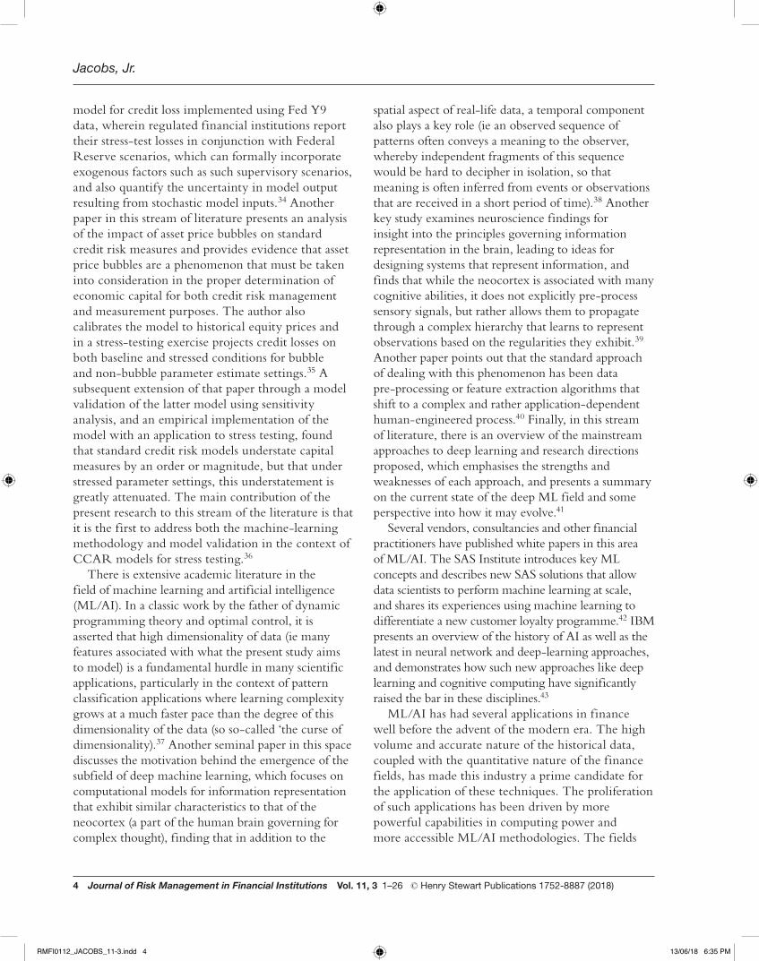
Finally, the paper turns to elements of the model validation process, focusing on elements that may or may not differ in the context of ML/AI modelling

methodologies and techniques. Figure 1 depicts the model validation function as the nexus of four core components (data, methodology, processes and governance), and two dimensions in the spectrum from quantitative to qualitative validation methodology. The figure highlights examples of some differences in the context of ML/AI modelling methodology. Clearly, many of the validation elements associated with traditional models will carry over to the ML/AI context, where they can be extended or differently emphasised.44

ECONOMETRIC METHODOLOGIESMacroeconomic forecasting sets out to achieve four basic tasks: characterise macroeconomic time series, conduct forecasts of macroeconomic or related data, make inferences about the structure of the economy, and finally advise policy-makers.45 The application of stress testing is mainly concerned with the forecasting and policy advisory functions, as stressed loss projections help banking risk managers and banking supervisors make decisions about

Figure 1: The model validation function and challenges in ML/AI modelling methodologies

• Is the devolopment sample appropriately chosen?• Is the quality of the data sufficient enough to develop a model?• Is the data being transferred correctly between the systems?

• Do validation results support fit/calibration quality of the model?• Are there appropriate/relevant theories & assumptions supporting the model in place?

• Measures of fit or discrimination may have different interpretations• Greater emphasis on out-of-sample performance and stability metrics

• Are there robust governance policy frameworks for development, ongoing monitoring and use of the models?• Is there a set mechanism for annual review and performance monitoring?

• It will be challenging to design policies, and knowledgeable governance, of more complex development, monitoring and use

ML/AI Techniques:

ML/AI Techniques:

Quantitative Validation

Qualitative Validation

Data Methodology

ValidationAreas

Processes Governance

• Are the processes efficient enough to secure an effective model execution?• Is the modeling process documented with sufficient developmental evidence?

• Greater complexity and computational overhead in model execution• More complex algorithms and model development processes to document

• Greater volume and less structure to data• Greater computational needs for integrity testing

Traditional Techniques: Traditional Techniques:

Traditional Techniques:Traditional Techniques:

ML/AI Techniques:

ML/AI Techniques:


Jacobs, Jr.


the potential viability of their institutions during periods of extreme economic turmoil. Going back a few decades, these functions were accomplished by a variety of means, ranging from large-scale models featuring the interactions of many variables, to simple univariate relationships motivated by stylised and parsimonious theories (eg Okun’s Law or the Phillips Curve). However, following the economic crises of the 1970s, most established economic relationships started to break down and these methods proved themselves to be unreliable. In the early 1980s, a new macroeconometric paradigm started to take hold — VAR, a simple yet f lexible way to model and forecast macroeconomic relationships.46 In contrast to the univariate autoregressive model,47,48 a VAR model is a multi-equation linear model in which variables can be explained by their own lags, as well as the lags of other variables. As with the application of CCAR/stress testing, what is of particular interest is modelling the relationship and forecasting multiple macroeconomic variables. To this end, the VAR methodology is rather suitable.

Let Yt = (Ylt,...,Ykt)T be a k-dimensional vector-

valued time series, the output variables of interest, in the present application, with the entries representing some loss measure in a particular segment, which may be inf luenced by a set of observable input variables denoted by Xt = (X lt,...,Xrt)

T , an r-dimensional vector-valued time series also referred to as exogenous variables, and in the present context representing a set of macroeconomic factors. This gives rise to the VARMAX (p,q,s) (vector autoregressive-moving average with exogenous variables) representation:

EB B BY X( ) ( ) ( )t t t

*Φ Θ Θ= + (1)

which is equivalent to:

Φ Θ Θ− =∑ ∑ + −∑−

=−

=−

=Y Y X E E

t j t jj

p

j t jj

s

t j t jj

q

1 0

*

1 (2)

where B BI( ) ,r j

j

j

p

1Φ Φ= −∑

= B B( )

jj

j

s

0Θ Θ= ∑

= and

B BI( )r j

j

j

q*

1Θ Θ= −∑

=

are autoregressive lag

polynomials of respective orders p, s and q, respectively, and B is the back-shift operator that

satisfies BiXt = Xt−i for any process {Xt}. It is common to assume that the input process Xt is generated independently of the noise process Et = (E1t,...,Ekt)

T. In fact, the exogenous variables {Xt} can represent both stochastic and non-stochastic (deterministic) variables, examples being sinusoidal seasonal (periodic) functions of time, used to represent the seasonal f luctuations in the output process {Yt}, or intervention analysis modelling in which a simple step (or pulse indicator) function takes the values of 0 or 1 to indicate the effect of output due to unusual intervention events in the system.

The autoregressive parameter matrices Φj represent sensitivities of output variables to their own lags and to lags of other output variables, while the corresponding matrices Θj are model sensitivities of output variables to contemporaneous and lagged values of input variables. Note that the VARMAX model (1)–(2) could be written in various equivalent forms, involving a lower triangular coefficient matrix for Yt at lag zero, or a leading coefficient matrix for εt at lag zero, or even a more general form that contains a leading (non-singular) coefficient matrix for Yt at lag zero that ref lects instantaneous links among the output variables that are motivated by theoretical considerations (provided that the proper identifiability conditions are satisfied).49–51 In the econometrics setting, such a model form is usually referred to as a dynamic simultaneous equations model or a dynamic structural equation model. The related model of this form is obtained by multiplying the dynamic simultaneous equations model form by the inverse of the lag 0 coefficient matrix, is referred to as the reduced form model. In addition, this model has a state space representation.52

It follows that the dependency structure of the output variables Yt, as given by the autocovariance function, is dependent upon the parameters Xt, and hence the correlations among the Yt as well as the correlation among the Xt that depend upon the parameters Θj. In contrast, in a system of univariate ARMAX (p,q,s) (autoregressive-moving average with exogenous variables) models, the correlations among the Yt are not taken into account, hence the parameter vectors Θj have a diagonal structure.




This study considers a vector autoregressive model with exogenous variables (VARX), denoted by VARX (p,s), which restricts the moving average (MA) terms beyond lag zero to be zero, or Θ∗

j = 0k×k j > 0:

Φ Θ− =∑ ∑ +−

=−

=Y Y X E

t j t jj

p

j t jj

s

t1 1

(3)

The rationale for this restriction is three-fold. First, with respect to MA terms, no cases were significant in the model estimations, so the data simply do not support a VARMAX representation. Secondly, using the VARX model provides the opportunity the very convenient DSE package in R, which has computational and analytical advantages.53 Finally, the VARX framework is more practical and intuitive than the more elaborate VARMAX model, and allows for superior communication of results to practitioners.

The paper now considers a machine-learning methodology, MARS, an adaptive procedure for regression that is well suited for high-dimensional problems.54 MARS can be viewed as a generalisation of stepwise linear regression or a modification of the classification and regression tree (CART) method to improve the latter’s performance in the regression setting. MARS uses expansions in piecewise linear basis functions of the form:

x t x t if x t

otherwise0,( )− = − >

+

(4)

and:

x t x t if x t

otherwise0.( )− = − <

−

(5)

Therefore, each function is piecewise linear, with a knot at the value, known as a linear spline. The two functions (4) and (5) are a ref lected pair, and the idea is to form such pairs for each input Xj, with knots at each observed value Xij of that input. The collection of basis functions is given by:

X t t X( ) ,( ) .j j t x x

j p,...,

1,...,j Nj1

{ }= − − { }+ +

∈=

(6)

If all of the input values are distinct, then there 2Np are basis functions altogether. Note that although

each basis function depends only on a single Xj , it is considered as a function over the entire input space p. Therefore, while the modelling strategy is similar to a forward stepwise linear regression, in lieu of using the original inputs there is the f lexibility to use functions from the set and their products. Here, the model takes the form:

β β= + ∑

=f X h X( ) ( ),

m mm

M

01

(7)

where each hm(X) is a function in p×N, or a product of two or more such functions, and given a choice for the such functions, the coefficients βm are estimated by standard linear regression. However, the power of this method lies in the design of the basis functions. The algorithm is initiated with a constant function h0(X) = 1 while the set functions in the set are considered as candidate functions. At each stage, all products of a function hm(X) in the model set M, together with one of the ref lected pairs in , are considered as a new basis function pair. The term of the following form is added to the model set M to produce the largest decrease in training error:

β β− + − ∈+

++

+h X X t h X t X hˆ ( )( ) ˆ ( )( ) , MM l j M l j l1 2

(8)

In Equation (8), M + 1 and M + 2 are coefficients estimated by least squares, along with all the other M + 1 coefficients in the model. Then the winning products are added to the model and the process is continued until the model set M contains some preset maximum number of terms. At the end of this process, a large model of this form typically over-fits the data, hence a backward deletion procedure is applied. The term whose removal causes the smallest increase in residual squared error is deleted from the model at each stage, producing an estimated best model of each size (ie number of terms) A, which could be optimally estimated through a cross-validation procedure. However, for the sake of computational savings, the MARS procedure instead uses a generalised cross-validation (GCV) criterion, that is defined as:

λλ

=−∑

−

λ=GCV

y f x

MN

( )( ˆ ( ))

1 ( )

i ii

N

12

(9)


Jacobs, Jr.


The value M (λ) is the effective number of parameters in the model, accounting both for the number of terms in the models, as well as the number of parameters used in selecting the optimal positions of the knots. As some mathematical and simulation results suggest that one should pay a price of three parameters for selecting a knot in a piecewise linear regression, it follows that if there are r linearly independent basis functions in the model, and K knots were selected in the forward process, the formula is M(λ) = r + CK, where C = 3. Using this, the model along the backward sequence that minimises GCV(λ) is selected.

The modelling strategy rationale for these piecewise linear basis functions is linked to the key property of this class of functions, namely their ability to operate locally. That is, they are zero over part of their range, but when multiplied together the result is nonzero over the small part of the feature space where both component functions are nonzero. In other words, the regression surface is built up parsimoniously using nonzero components locally only where they are needed. The importance of this lies in the principle that one should economise on parameters in high dimensions, as one can quickly face the curse of dimensionality in an exploding parameter space, as in the use of other basis functions such as polynomials that produce nonzero product everywhere and become quickly intractable. Another key advantage of the piecewise linear basis function concerns a significantly reduced computational overhead. Consider the product of a function in M with each of the N ref lected pairs for an input Xj, which appears to require the fitting of N single-input linear regression models, each of which uses O(N) operations, making a total of O(N 2) operations. However, one can exploit the simple form of the piecewise linear function by first fitting the ref lected pair with the rightmost knot, and as the knot is moved successively to the left, one position at a time, the basis functions differ by zero over the left part of the domain and by a constant over the right part. Therefore, after each such move, one can update the fit in O(1) operations, which makes it possible to try every knot in only O(N ) operations. The forward modelling strategy in MARS is hierarchical, in the sense that multiway products are built up from products involving terms already in the model.

While the theory that a high-order interaction will likely only exist if some of its lower-order versions exist as well need not be true, nevertheless this is a reasonable working assumption and avoids the search over an exponentially growing space of alternatives. Finally, note one restriction put on the formation of model terms, namely that each input can appear at most once in a product; this prevents the formation of higher-order powers of an input that may increase or decrease too sharply near the boundaries of the feature space. Such powers can be approximated in a more stable way with piecewise linear functions. In order to implement this, one can exploit a useful option in the MARS procedure that sets an upper limit on the order of interaction, which can aid in the interpretation of the final model (eg an upper limit of one results in an additive model).

EMPIRICAL IMPLEMENTATIONAs part of the Federal Reserve’s CCAR stress-testing exercise, US domiciled top-tier BHCs are required to submit comprehensive capital plans, including pro forma capital analyses, based on at least one BHC-defined adverse scenario. The adverse scenario is described by quarterly trajectories for key macroeconomic variables over the next nine quarters or for 13 months to estimate loss allowances. In addition, the Federal Reserve generates its own supervisory stress scenarios, so that firms are expected to apply both BHC and supervisory stress scenarios to all exposures, in order to estimate potential losses under stressed operating conditions. Firms engaged in significant trading activities (eg Goldman Sachs or Morgan Stanley) are asked to estimate a one-time trading-related market and counterparty credit loss shock under their own BHC scenarios, and a market risk stress scenario provided by the supervisors. Large custodian banks are asked to estimate the potential default of their largest counterparty. In the case of the supervisory stress scenarios, the Federal Reserve provides firms with global market shock components that are one-time, hypothetical shocks to a large set of risk factors. During the last two CCAR exercises, these shocks involved large and sudden changes in asset prices, rates, and CDS spreads that mirrored the severe market conditions in the second half of 2008.




As CCAR is a comprehensive assessment of a firm’s capital plan, the BHCs are asked to conduct an assessment of the expected uses and sources of capital over a planning horizon. In the 2009 SCAP, firms were asked to submit stress losses over the next two years, on a yearly basis. Since then, the planning horizon has changed to nine quarters. For the last three CCAR exercises, BHCs are asked to submit their pro forma, post-stress capital projections in their capital plan beginning with data as of 30th September, spanning the nine-quarter planning horizon. The projections begin in the fourth quarter of the current year and conclude at the end of the fourth quarter two years forward. Hence, for defining BHC stress scenarios, firms are asked to project the movements of key macroeconomic variables over the planning horizon of nine quarters. Determination of the severity of the global market shock components for trading and counterparty credit losses will not be discussed in this paper, because it is a one-time shock and the evaluation will be on the movements of the market risk factors rather the macroeconomic variables. In the 2011 CCAR, the Federal Reserve defined the stress supervisory scenario using nine macroeconomic variables:

• real GDP growth (RGDPG); • consumer price index (CPI); • real disposable personal income (RDPI); • unemployment rate (UNEMP); • three-month treasury bill rate (3MTBR); • five-year treasury bond rate (5YTBR); • ten-year treasury bond rate (10YTBR); • BBB corporate rate (BBBCR); • Dow Jones Index (DJI); and • national house price index (HPI).

In CCAR 2012, the number of macroeconomic variables that defined the supervisory stress scenario increased to 15. In addition to the original nine variables, the following variables were added:

• nominal disposable income growth (NDPIG); • mortgage rate (MR); • CBOE’s market volatility index (VIX); • commercial real estate price index (CREPI); and • prime rate (PR).

For CCAR 2013, the Federal Reserve System used the same set of variables to define the supervisory adverse scenario as in 2012. Additionally, there was another set of 12 international macroeconomic variables, three macroeconomic variables and four countries/country blocs, included in the supervisory stress scenario. For the purposes of the present research, consider the supervisory scenarios from 2016, in conjunction with the following calculated interest rate spreads:

• ten-year treasury minus three-month treasury spread or term spread (TS); and

• BBB corporate rate minus five-year treasury spread or corporate spread (CS).

Therefore, a diverse set of macroeconomic drivers representing varied dimensions of the economic environment, and a sufficient number of drivers balancing the consideration of avoiding over-fitting industry standards (ie at least 2–3 and no more than 5–7 independent variables) are considered. This model selection is performed using an R script designed for this purpose, using the libraries ‘dse’ and ‘tse’ to estimate and evaluate VARMAX and ARMAX models, and the ‘Earth’ package for the MARS models (R Core Development Team, 2016). The model selection process imposes the following criteria in selecting input and output variables across both multiple VARMAX/univariate ARMAX and MARS models:

• transformations of chosen variables should indicate stationarity;

• signs of coefficient estimates are economically intuitive;

• probability values of coefficient estimates indicate statistical significance at conventional confidence levels;

• residual diagnostics indicate white noise behaviour; and

• model performance metrics (goodness of fit, risk ranking and cumulative error measures) are within industry accepted thresholds of acceptability. Scenarios rank order intuitively (ie severely adverse scenario stress losses exceeding scenario base expected losses).


Jacobs, Jr.


Similarly, the following loss segments (with loss measured by gross net charge-off rates) are identified according to the same criteria, in conjunction with the requirement that they cover the most prevalent portfolio types in typical traditional banking institutions:

• commercial and industrial (C&I); • commercial real estate (CRE); and • consumer credit (CONS).

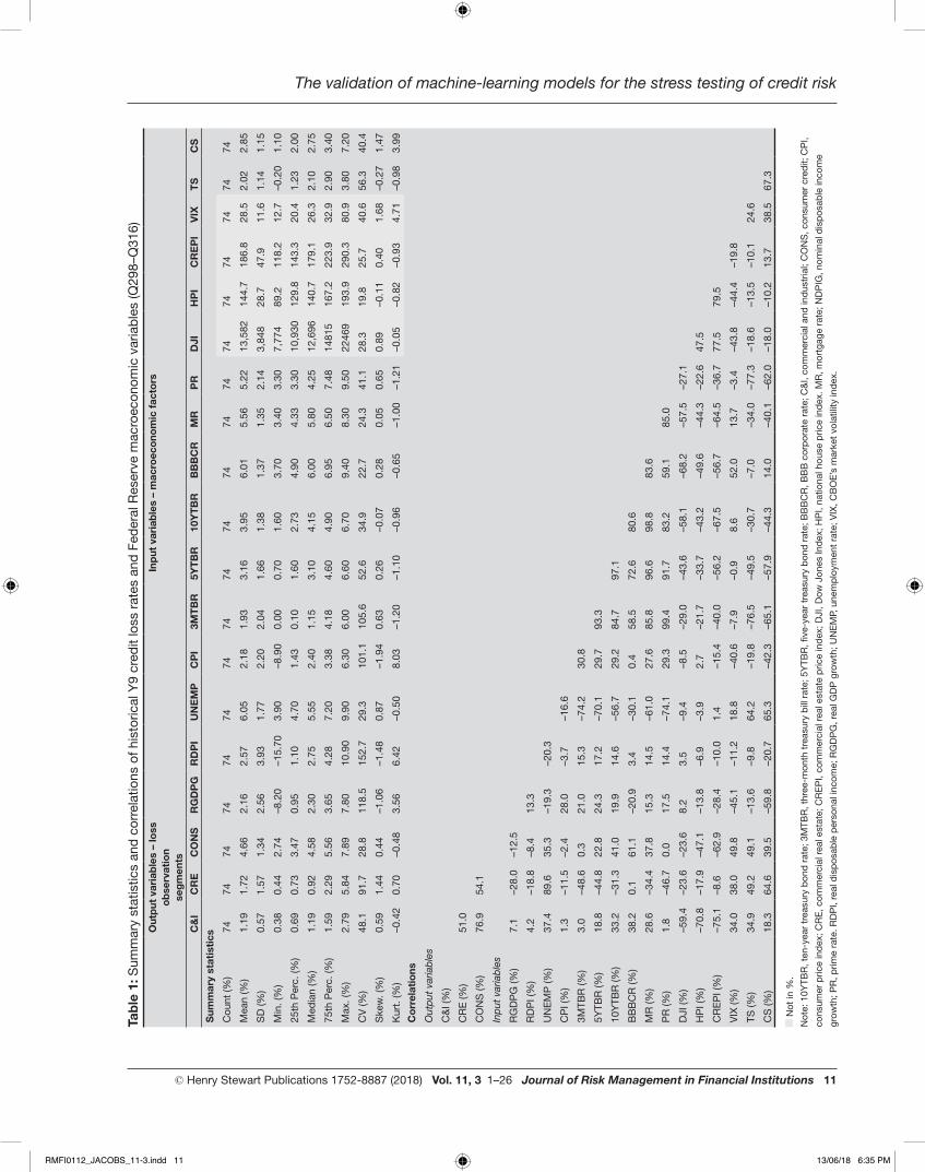
The historical data — 74 quarterly observations from 2Q98 to 3Q16 — are summarised in Table 1 in terms of distributional statistics and correlations. First, the paper will describe the main features of the dependency structure within the group of input macroeconomic variables, then the same for the output loss rate variables, and finally the cross-correlations between these two groups. One can observe that all correlations have intuitive signs and magnitudes that suggest significant relationships, although the latter are not large enough to suggest any issues with multicollinearity.

The correlation matrix among the macroeconomic variables appears in the lower-right quadrant of the bottom panel of Table 1. For example, considering some of the stronger relationships among the levels, the correlations between UNEMP/CS, RGDPG/VIX and DOW/CREPI are 65.3 per cent, –45.1 per cent and 77.5 per cent, respectively. The correlation matrix among the credit loss rate variables appears in the upper-left quadrant of the bottom panel of Table 1. The correlations between CRE/CNI, CONS/CNI and CRE/CONS are 51.0 per cent, 78.9 per cent and 54.1 per cent, respectively. The correlation matrix among the credit loss rate and macroeconomic variables appears in the lower-left quadrant of the bottom panel of Table 1. For example, considering some of the stronger relationships among the levels, the correlations between UNEMP/CRE, CREPI/CNI and BBBCY/CONS are 89.6 per cent, –75.1 per cent and 61.1 per cent, respectively.

In the case of C&I, the best model for the quarterly change in net charge-off rates was found, according to the model selection process, to contain the transformations of the following macroeconomic variables:

• RGDP: lagged four quarters; and • CS: two-quarter change lagged four quarters.

In the case of CRE, the best corresponding model is found to be:

• BBB corporate yield: four-quarter change lagged two quarters; and

• unemployment rate: lagged one quarter.

In the case of CONS, the best corresponding model is found to be:

• BBB corporate yield: three-quarter change lagged four quarters; and

• unemployment rate: lagged one quarter.

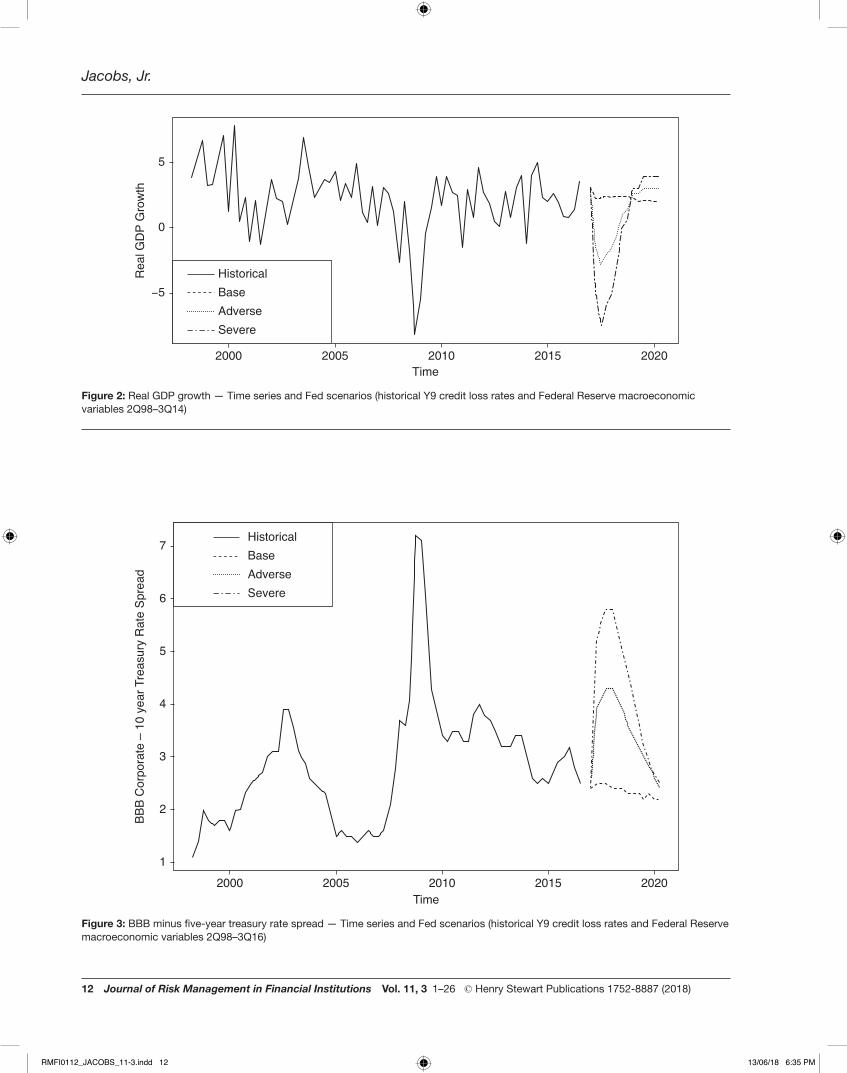
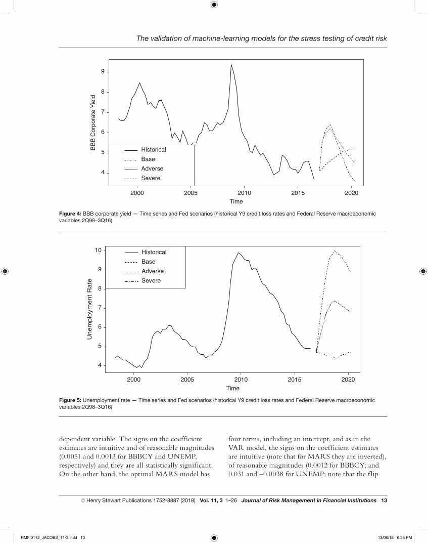
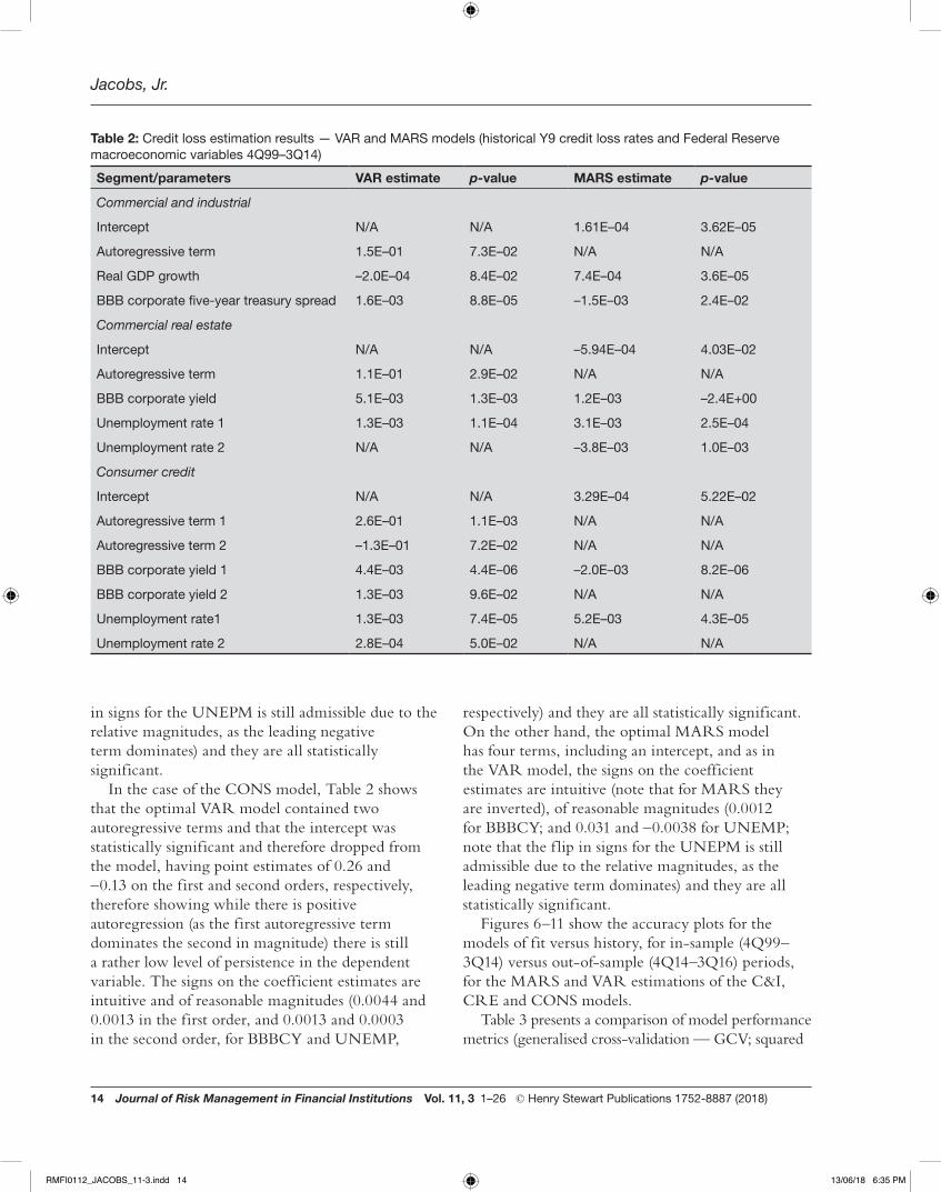
The time series and Fed scenario forecasts of RDGP, CS, BBBCR and UNEMP are shown in Figures 2–5, and the estimation results (parameter estimates and p-values) for the VAR and MARS estimation are shown in Table 2.

In the case of the C&I model, Table 2 shows that the optimal VAR model contained only a single autoregressive term and that the intercept was statistically significant and therefore dropped from the model, having a point estimate of 0.15, therefore showing that while there is positive autoregression, there is still a rather low level of persistence in the dependent variable. The signs on the coefficient estimates are intuitive and of reasonable magnitudes (–0.0002 and 0.0016 for RGDP and CS, respectively) and they are all statistically significant. On the other hand, the optimal MARS model has three terms including an intercept (the so-called effective number of parameters is three), and as in the VAR model the signs on the coefficient estimates are intuitive (note that that for MARS they are inverted), of reasonable magnitudes (0.0007 and –0.0015 for RGDP and CS, respectively) and they are all statistically significant.

In the case of the CRE model, Table 2 shows that the optimal VAR model contained only a single autoregressive term and that the intercept was statistically significant and therefore dropped from the model, having a point estimate of 0.11, therefore showing that while there is positive autoregression, there is still a rather low level of persistence in the




Tab

le 1

: Sum

mar

y st

atis

tics

and

corre

latio

ns o

f his

toric

al Y

9 cr

edit

loss

rate

s an

d Fe

dera

l Res

erve

mac

roec

onom

ic v

aria

bles

(Q29

8–Q

316)

Out

put

var

iab

les

– lo

ss

ob

serv

atio

nse

gm

ents

Inp

ut v

aria

ble

s –

mac

roec

ono

mic

fac

tors

C&

IC

RE

CO

NS

RG

DP

GR

DP

IU

NE

MP

CP

I3M

TB

R5Y

TB

R10

YT

BR

BB

BC

RM

RP

RD

JIH

PI

CR

EP

IV

IXT

SC

S

Sum

mar

y st

atis

tics

Cou

nt (%

)74

7474

7474

7474

7474

7474

7474

7474

7474

7474

Mea

n (%

)1.

191.

724.

662.

162.

576.

052.

181.

933.

163.

956.

015.

565.

2213

,582

144.

718

6.8

28.5

2.02

2.85

SD (%

)0.

571.

571.

342.

563.

931.

772.

202.

041.

661.

381.

371.

352.

143,

848

28.7

47.9

11.6

1.14

1.15

Min

. (%

)0.

380.

442.

74–8

.20

–15.

703.

90–8

.90

0.00

0.70

1.60

3.70

3.40

3.30

7,77

489

.211

8.2

12.7

–0.2

01.

1025

th P

erc.

(%)

0.69

0.73

3.47

0.95

1.10

4.70

1.43

0.10

1.60

2.73

4.90

4.33

3.30

10,9

3012

9.8

143.

320

.41.

232.

00M

edia

n (%

)1.

190.

924.

582.

302.

755.

552.

401.

153.

104.

156.

005.

804.

2512

,696

140.

717

9.1

26.3

2.10

2.75

75th

Per

c. (%

)1.

592.

295.

563.

654.

287.

203.

384.

184.

604.

906.

956.

507.

4814

815

167.

222

3.9

32.9

2.90

3.40

Max

. (%

)2.

795.

847.

897.

8010

.90

9.90

6.30

6.00

6.60

6.70

9.40

8.30

9.50

2246

919

3.9

290.

380

.93.

807.

20C

V (%

)48

.191

.728

.811

8.5

152.

729

.310

1.1

105.

652

.634

.922

.724

.341

.128

.319

.825

.740

.656

.340

.4Sk

ew. (

%)

0.59

1.44

0.44

–1.0

6–1

.48

0.87

–1.9

40.

630.

26–0

.07

0.28

0.05

0.65

0.89

–0.1

10.

401.

68–0

.27

1.47

Kurt.

(%)

–0.4

20.

70–0

.48

3.56

6.42

–0.5

08.

03–1

.20

–1.1

0–0

.96

–0.6

5–1

.00

–1.2

1–0

.05

–0.8

2–0

.93

4.71

–0.9

83.

99C

orr

elat

ions

Out

put v

aria

bles

C&I

(%)

CRE

(%)

51.0

CO

NS

(%)

76.9

54.1

Inpu

t var

iabl

esRG

DPG

(%)

7.1

–28.

0–1

2.5

RDPI

(%)

4.2

–18.

8–8

.413

.3U

NEM

P (%

)37

.489

.635

.3–1

9.3

–20.

3C

PI (%

)1.

3–1

1.5

–2.4

28.0

–3.7

–16.

63M

TBR

(%)

3.0

–48.

60.

321

.015

.3–7

4.2

30.8

5YTB

R (%

)18

.8–4

4.8

22.8

24.3

17.2

–70.

129

.793

.310

YTBR

(%)

33.2

–31.

341

.019

.914

.6–5

6.7

29.2

84.7

97.1

BBBC

R (%

)38

.20.

161

.1–2

0.9

3.4

–30.

10.

458

.572

.680

.6M

R (%

)28

.6–3

4.4

37.8

15.3

14.5

–61.

027

.685

.896

.698

.883

.6PR

(%)

1.8

–46.

70.

017

.514

.4–7

4.1

29.3

99.4

91.7

83.2

59.1

85.0

DJI (

%)

–59.

4–2

3.6

–23.

68.

23.

5–9

.4–8

.5–2

9.0

–43.

6–5

8.1

–68.

2–5

7.5

–27.

1H

PI (%

)–7

0.8

–17.

9–4

7.1

–13.

8–6

.9–3

.92.

7–2

1.7

–33.

7–4

3.2

–49.

6–4

4.3

–22.

647

.5C

REPI

(%)

–75.

1–8

.6–6

2.9

–28.

4–1

0.0

1.4

–15.

4–4

0.0

–56.

2–6

7.5

–56.

7–6

4.5

–36.

777

.579

.5VI

X (%

)34

.038

.049

.8–4

5.1

–11.

218

.8–4

0.6

–7.9

–0.9

8.6

52.0

13.7

–3.4

–43.

8–4

4.4

–19.

8TS

(%)

34.9

49.2

49.1

–13.

6–9

.864

.2–1

9.8

–76.

5–4

9.5

–30.

7–7

.0–3

4.0

–77.

3–1

8.6

–13.

5–1

0.1

24.6

CS

(%)

18.3

64.6

39.5

–59.

8–2

0.7

65.3

–42.

3–6

5.1

–57.

9–4

4.3

14.0

–40.

1–6

2.0

–18.

0–1

0.2

13.7

38.5

67.3

Not

in %

. N

ote:

10Y

TBR,

ten-

year

trea

sury

bon

d ra

te; 3

MTB

R, th

ree-

mon

th tr

easu

ry b

ill ra

te; 5

YTBR

, five

-yea

r tre

asur

y bo

nd ra

te; B

BBC

R, B

BB c

orpo

rate

rate

; C&I

, com

mer

cial

and

indu

stria

l; C

ON

S, c

onsu

mer

cre

dit;

CPI

, co

nsum

er p

rice

inde

x; C

RE, c

omm

erci

al re

al e

stat

e; C

REPI

, com

mer

cial

real

est

ate

pric

e in

dex;

DJI

, Dow

Jon

es In

dex;

HPI

, nat

iona

l hou

se p

rice

inde

x. M

R, m

ortg

age

rate

; NDP

IG, n

omin

al d

ispo

sabl

e in

com

e gr

owth

; PR,

prim

e ra

te. R

DPI,

real

dis

posa

ble

pers

onal

inco

me;

RG

DPG

, rea

l GDP

gro

wth

; UN

EMP,

une

mpl

oym

ent r

ate;

VIX

, CBO

E’s

mar

ket v

olat

ility

inde

x.


Jacobs, Jr.


2010Time

2015 20202000

−5

5

0

Rea

l GD

P G

row

th

2005

Historical

Base

Adverse

Severe

Figure 2: Real GDP growth — Time series and Fed scenarios (historical Y9 credit loss rates and Federal Reserve macroeconomic variables 2Q98–3Q14)

Figure 3: BBB minus five-year treasury rate spread — Time series and Fed scenarios (historical Y9 credit loss rates and Federal Reserve macroeconomic variables 2Q98–3Q16)

2000

1

2

3

4

5

BBB

Cor

pora

te –

10

year

Tre

asur

y R

ate

Spre

ad

6

7

2005 2010Time

2015 2020

HistoricalBaseAdverseSevere




Figure 5: Unemployment rate — Time series and Fed scenarios (historical Y9 credit loss rates and Federal Reserve macroeconomic variables 2Q98–3Q16)

Figure 4: BBB corporate yield — Time series and Fed scenarios (historical Y9 credit loss rates and Federal Reserve macroeconomic variables 2Q98–3Q16)

2005 2010Time

2015 20202000

4

5

6

7

8

9

BBB

Cor

pora

te Y

ield


2005 2010Time

2015 20202000

4

5

6

7

8

9

10

Une

mpl

oym

ent R

ate


dependent variable. The signs on the coefficient estimates are intuitive and of reasonable magnitudes (0.0051 and 0.0013 for BBBCY and UNEMP, respectively) and they are all statistically significant. On the other hand, the optimal MARS model has

four terms, including an intercept, and as in the VAR model, the signs on the coefficient estimates are intuitive (note that for MARS they are inverted), of reasonable magnitudes (0.0012 for BBBCY; and 0.031 and –0.0038 for UNEMP; note that the f lip


Jacobs, Jr.


in signs for the UNEPM is still admissible due to the relative magnitudes, as the leading negative term dominates) and they are all statistically significant.

In the case of the CONS model, Table 2 shows that the optimal VAR model contained two autoregressive terms and that the intercept was statistically significant and therefore dropped from the model, having point estimates of 0.26 and –0.13 on the first and second orders, respectively, therefore showing while there is positive autoregression (as the first autoregressive term dominates the second in magnitude) there is still a rather low level of persistence in the dependent variable. The signs on the coefficient estimates are intuitive and of reasonable magnitudes (0.0044 and 0.0013 in the first order, and 0.0013 and 0.0003 in the second order, for BBBCY and UNEMP,

respectively) and they are all statistically significant. On the other hand, the optimal MARS model has four terms, including an intercept, and as in the VAR model, the signs on the coefficient estimates are intuitive (note that for MARS they are inverted), of reasonable magnitudes (0.0012 for BBBCY; and 0.031 and –0.0038 for UNEMP; note that the f lip in signs for the UNEPM is still admissible due to the relative magnitudes, as the leading negative term dominates) and they are all statistically significant.

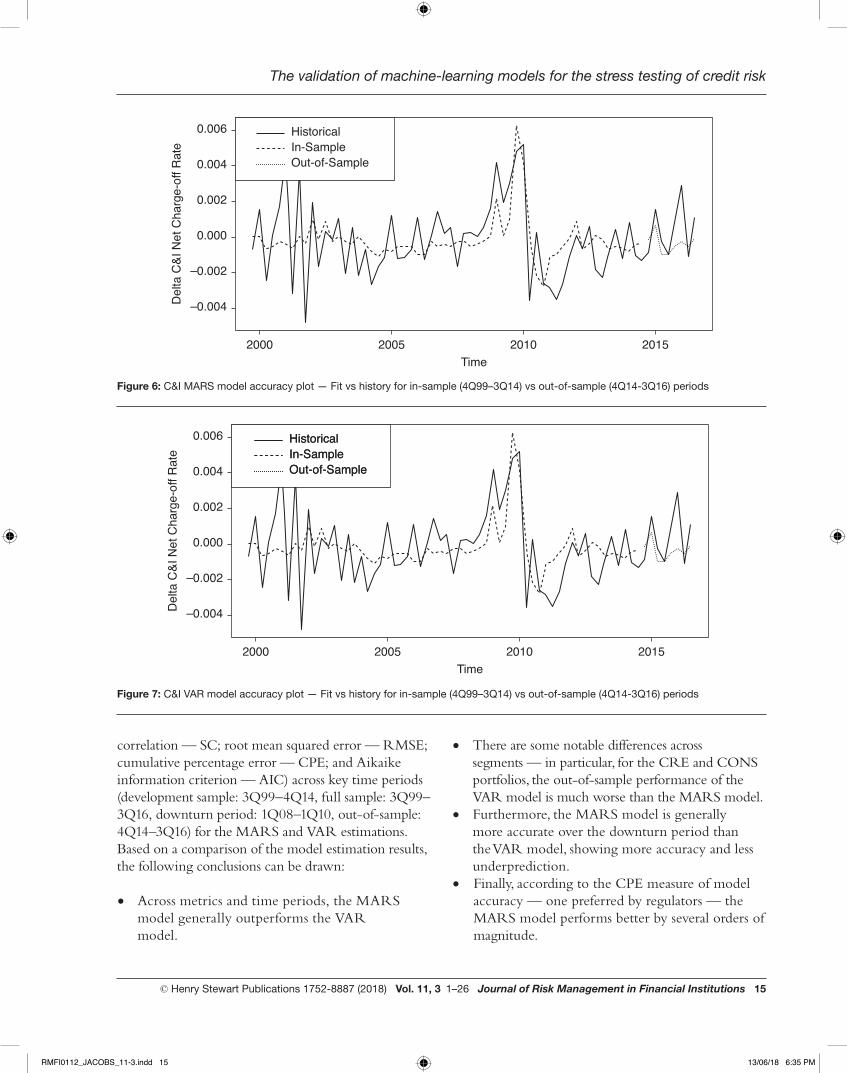
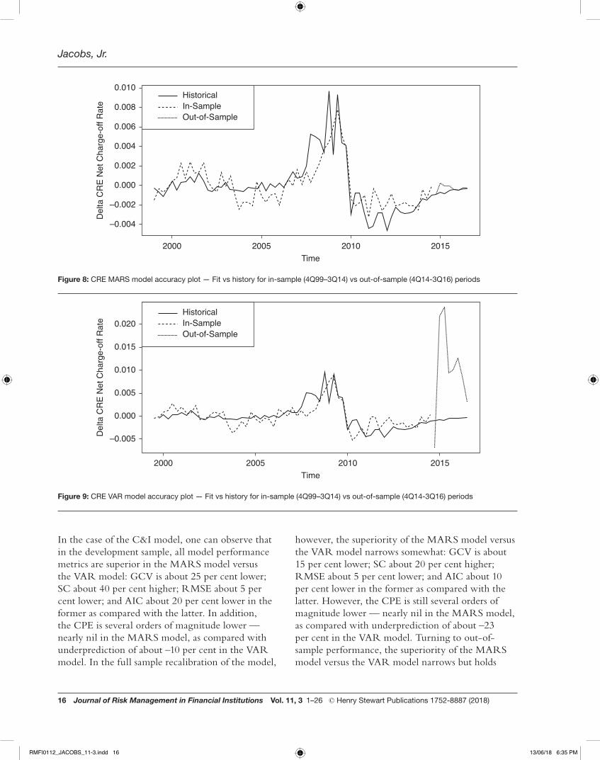
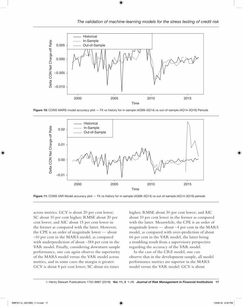
Figures 6–11 show the accuracy plots for the models of fit versus history, for in-sample (4Q99–3Q14) versus out-of-sample (4Q14–3Q16) periods, for the MARS and VAR estimations of the C&I, CRE and CONS models.

Table 3 presents a comparison of model performance metrics (generalised cross-validation — GCV; squared

Table 2: Credit loss estimation results — VAR and MARS models (historical Y9 credit loss rates and Federal Reserve macroeconomic variables 4Q99–3Q14)Segment/parameters VAR estimate p-value MARS estimate p-value

Commercial and industrial

Intercept N/A N/A 1.61E–04 3.62E–05

Autoregressive term 1.5E–01 7.3E–02 N/A N/A

Real GDP growth –2.0E–04 8.4E–02 7.4E–04 3.6E–05

BBB corporate five-year treasury spread 1.6E–03 8.8E–05 –1.5E–03 2.4E–02

Commercial real estate

Intercept N/A N/A –5.94E–04 4.03E–02

Autoregressive term 1.1E–01 2.9E–02 N/A N/A

BBB corporate yield 5.1E–03 1.3E–03 1.2E–03 –2.4E+00

Unemployment rate 1 1.3E–03 1.1E–04 3.1E–03 2.5E–04

Unemployment rate 2 N/A N/A –3.8E–03 1.0E–03

Consumer credit

Intercept N/A N/A 3.29E–04 5.22E–02

Autoregressive term 1 2.6E–01 1.1E–03 N/A N/A

Autoregressive term 2 –1.3E–01 7.2E–02 N/A N/A

BBB corporate yield 1 4.4E–03 4.4E–06 –2.0E–03 8.2E–06

BBB corporate yield 2 1.3E–03 9.6E–02 N/A N/A

Unemployment rate1 1.3E–03 7.4E–05 5.2E–03 4.3E–05

Unemployment rate 2 2.8E–04 5.0E–02 N/A N/A




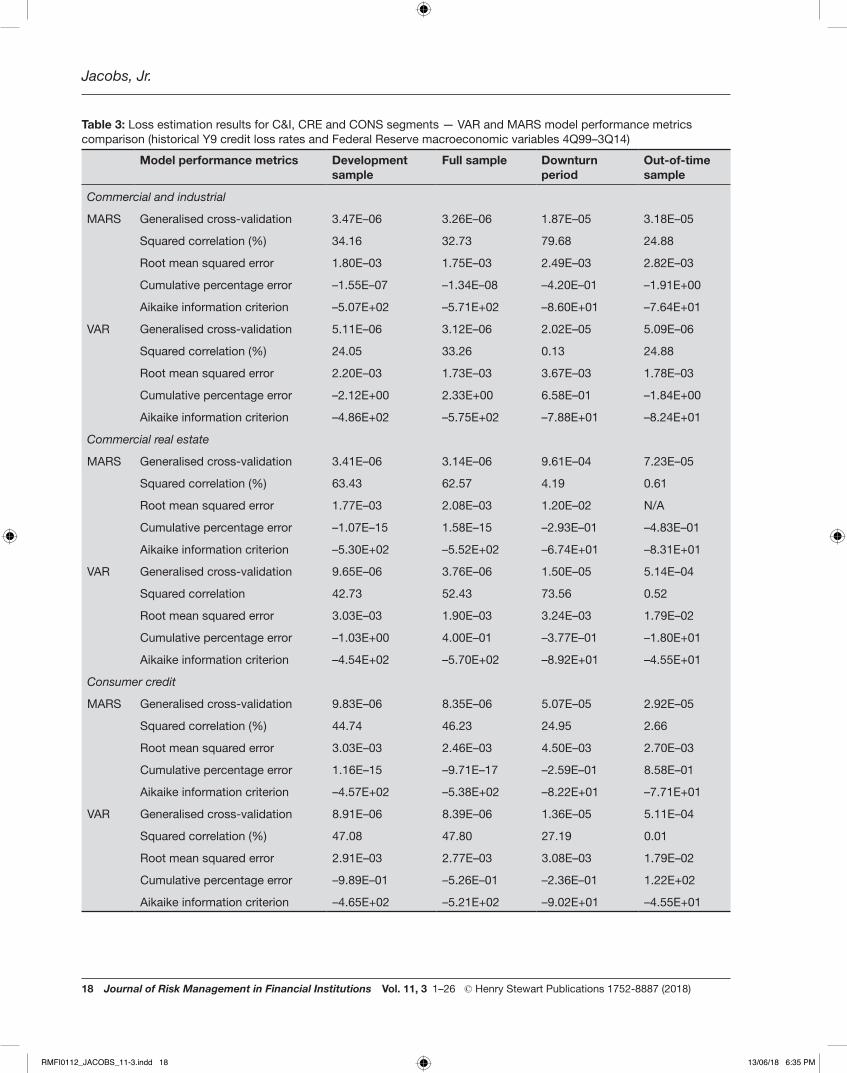
correlation — SC; root mean squared error — RMSE; cumulative percentage error — CPE; and Aikaike information criterion — AIC) across key time periods (development sample: 3Q99–4Q14, full sample: 3Q99–3Q16, downturn period: 1Q08–1Q10, out-of-sample: 4Q14–3Q16) for the MARS and VAR estimations. Based on a comparison of the model estimation results, the following conclusions can be drawn:

• Across metrics and time periods, the MARS model generally outperforms the VAR model.

• There are some notable differences across segments — in particular, for the CRE and CONS portfolios, the out-of-sample performance of the VAR model is much worse than the MARS model.

• Furthermore, the MARS model is generally more accurate over the downturn period than the VAR model, showing more accuracy and less underprediction.

• Finally, according to the CPE measure of model accuracy — one preferred by regulators — the MARS model performs better by several orders of magnitude.

2005 2010Time

20152000

–0.004

–0.002

0.000

0.002

Del

ta C

&I N

et C

harg

e-of

f Rat

e0.004

0.006 HistoricalIn-SampleOut-of-Sample

Figure 6: C&I MARS model accuracy plot — Fit vs history for in-sample (4Q99–3Q14) vs out-of-sample (4Q14-3Q16) periods

2005 2010Time

20152000

–0.004

–0.002

0.000

0.002

Del

ta C

&I N

et C

harg

e-of

f Rat

e

0.004

0.006 HistoricalIn-SampleOut-of-Sample

HistoricalIn-SampleOut-of-Sample

Figure 7: C&I VAR model accuracy plot — Fit vs history for in-sample (4Q99–3Q14) vs out-of-sample (4Q14-3Q16) periods


Jacobs, Jr.


In the case of the C&I model, one can observe that in the development sample, all model performance metrics are superior in the MARS model versus the VAR model: GCV is about 25 per cent lower; SC about 40 per cent higher; RMSE about 5 per cent lower; and AIC about 20 per cent lower in the former as compared with the latter. In addition, the CPE is several orders of magnitude lower — nearly nil in the MARS model, as compared with underprediction of about –10 per cent in the VAR model. In the full sample recalibration of the model,

however, the superiority of the MARS model versus the VAR model narrows somewhat: GCV is about 15 per cent lower; SC about 20 per cent higher; RMSE about 5 per cent lower; and AIC about 10 per cent lower in the former as compared with the latter. However, the CPE is still several orders of magnitude lower — nearly nil in the MARS model, as compared with underprediction of about –23 per cent in the VAR model. Turning to out-of-sample performance, the superiority of the MARS model versus the VAR model narrows but holds

2005 2010Time

20152000

–0.004

–0.002

0.000

0.002

Del

ta C

RE

Net

Cha

rge-

off R

ate

0.004

0.006

0.010

0.008HistoricalIn-SampleOut-of-Sample

Figure 8: CRE MARS model accuracy plot — Fit vs history for in-sample (4Q99–3Q14) vs out-of-sample (4Q14-3Q16) periods

2005 2010Time

20152000

–0.005

0.000

0.005

0.010

0.015

Del

ta C

RE

Net

Cha

rge-

off R

ate 0.020


Figure 9: CRE VAR model accuracy plot — Fit vs history for in-sample (4Q99–3Q14) vs out-of-sample (4Q14-3Q16) periods




across metrics: GCV is about 20 per cent lower; SC about 10 per cent higher; RMSE about 20 per cent lower; and AIC about 15 per cent lower in the former as compared with the latter. However, the CPE is an order of magnitude lower — about –10 per cent in the MARS model, as compared with underprediction of about –184 per cent in the VAR model. Finally, considering downturn sample performance, one can again observe the superiority of the MARS model versus the VAR model across metrics, and in some cases the margin is greater: GCV is about 8 per cent lower; SC about six times

higher; RMSE about 30 per cent lower; and AIC about 10 per cent lower in the former as compared with the latter. Meanwhile, the CPE is an order of magnitude lower — about –4 per cent in the MARS model, as compared with over-prediction of about 66 per cent in the VAR model, the latter being a troubling result from a supervisory perspective regarding the accuracy of the VAR model.

In the case of the CRE model, one can observe that in the development sample, all model performance metrics are superior in the MARS model versus the VAR model: GCV is about

Figure 11: CONS VAR Model accuracy plot — Fit vs history for in-sample (4Q99–3Q14) vs out-of-sample (4Q14-3Q16) periods

2005 2010Time

20152000

–0.010

–0.005

0.000

Del

ta C

ON

Net

Cha

rge-

off R

ate

0.005


Figure 10: CONS MARS model accuracy plot — Fit vs history for in-sample (4Q99–3Q14) vs out-of-sample (4Q14-3Q16) Periods

2005 2010Time

20152000

–0.01

0.00

0.01

Del

ta C

ON

Net

Cha

rge-

off R

ate

0.02



Jacobs, Jr.


Table 3: Loss estimation results for C&I, CRE and CONS segments — VAR and MARS model performance metrics comparison (historical Y9 credit loss rates and Federal Reserve macroeconomic variables 4Q99–3Q14)

Model performance metrics Development sample

Full sample Downturn period

Out-of-time sample


MARS Generalised cross-validation 3.47E–06 3.26E–06 1.87E–05 3.18E–05

Squared correlation (%) 34.16 32.73 79.68 24.88

Root mean squared error 1.80E–03 1.75E–03 2.49E–03 2.82E–03

Cumulative percentage error –1.55E–07 –1.34E–08 –4.20E–01 –1.91E+00

Aikaike information criterion –5.07E+02 –5.71E+02 –8.60E+01 –7.64E+01

VAR Generalised cross-validation 5.11E–06 3.12E–06 2.02E–05 5.09E–06



Cumulative percentage error –2.12E+00 2.33E+00 6.58E–01 –1.84E+00





Root mean squared error 1.77E–03 2.08E–03 1.20E–02 N/A

Cumulative percentage error –1.07E–15 1.58E–15 –2.93E–01 –4.83E–01



Squared correlation 42.73 52.43 73.56 0.52


Cumulative percentage error –1.03E+00 4.00E–01 –3.77E–01 –1.80E+01


Consumer credit




Cumulative percentage error 1.16E–15 –9.71E–17 –2.59E–01 8.58E–01





Cumulative percentage error –9.89E–01 –5.26E–01 –2.36E–01 1.22E+02





30 per cent lower; SC about 50 per cent higher; RMSE about 40 per cent lower; and AIC about 17 per cent lower in the former as compared with the latter. In addition, the CPE is several orders of magnitude lower — nearly nil in the MARS model, as compared with underprediction of about –100 per cent in the VAR model. However, in the full sample recalibration of the model, the superiority of the MARS model versus the VAR model narrows somewhat: GCV is about 17 per cent lower; SC about 20 per cent higher; RMSE about 30 per cent lower; and AIC about 16 per cent lower in the former as compared with the latter. However, the CPE is still several orders of magnitudes lower — nearly nil in the MARS model, as compared with underprediction of about –23 per cent in the VAR model. Turning to out-of-sample performance, the superiority of the MARS model versus the VAR model is much amplified across metrics: GCV is about 86 per cent lower; SC about 18 per cent higher; RMSE about 20 per cent lower and AIC about 98 per cent lower in the former as compared with the latter. However, the CPE is an order of magnitude lower — about –5 per cent in the MARS model, as compared with overprediction of about 180 per cent in the VAR model. Finally, considering downturn sample performance, one can once again observe the superiority of the MARS model versus the VAR model across metrics, and in some cases the margin is greater: GCV is about 36 per cent lower; SC about 13 per cent higher; RMSE about 26 per cent lower; and AIC about 10 per cent lower in the former as compared with the latter. Meanwhile, the CPE is lower — about –29 per cent in the MARS model, as compared with underprediction of about –38 per cent in the VAR model.

In the case of the CONS model, one can observe that in the development sample, all model performance metrics are superior in the MARS model compared with the VAR model: GCV is about 45 per cent lower; SC about 14 per cent higher; RMSE about 20 per cent lower; and AIC about twice as low in the former as compared with the latter. Meanwhile, the CPE is several orders of magnitude lower — nearly nil in the MARS model, as compared with underprediction of about –99 per cent in the VAR model. However, in the full sample recalibration of the model, the superiority

of the MARS model compared with the VAR model narrows somewhat: GCV is about 50 per cent lower; SC about 16 per cent higher; RMSE about 10 per cent lower; and AIC about half as large in the former as compared with the latter. However, the CPE is still several orders of magnitude lower — nearly nil in the MARS model, as compared with underprediction of about –53 per cent in the VAR model. Turning to out-of-sample performance, the superiority of the MARS model compared with the VAR model is much amplified across metrics: GCV is about 94 per cent lower; SC over twice as high; RMSE about 85 per cent lower; and AIC about 170 per cent low in the former as compared with the latter. However, the CPE is an order of magnitude lower, about –9 per cent in the MARS model, as compared with overprediction of about 122 per cent in the VAR model. Finally, considering downturn sample performance, one can again observe the superiority of the MARS model compared with the VAR model across metrics, and in some cases the margin is greater: GCV is about 7 per cent lower; SC about 25 per cent higher; RMSE still about 20 per cent lower; and AIC about 20 per cent lower in the former as compared with the latter. Meanwhile, the CPE is lower — about –0.03 per cent in the MARS model, as compared with underprediction of about –0.05 per cent in the VAR model.

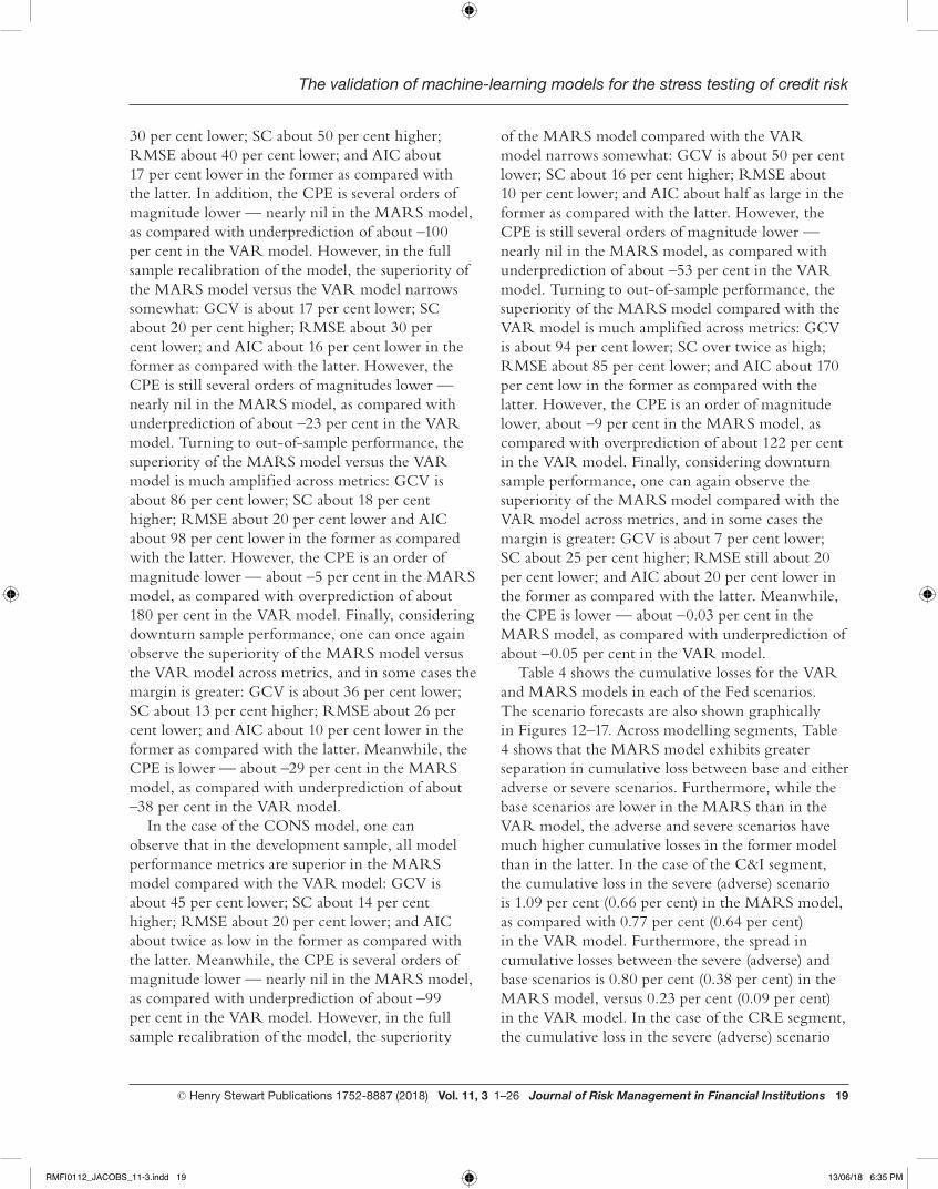
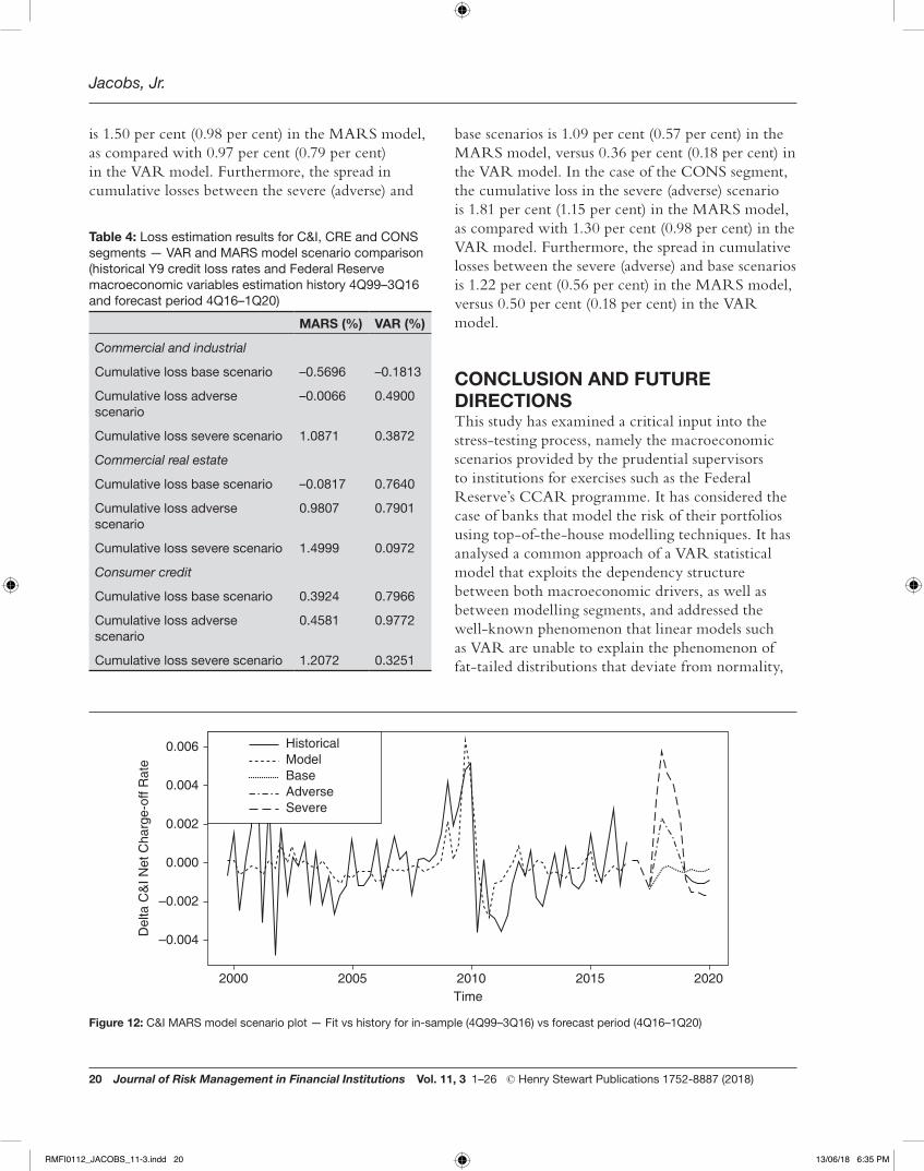
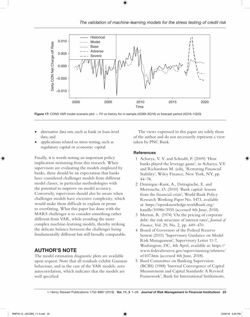
Table 4 shows the cumulative losses for the VAR and MARS models in each of the Fed scenarios. The scenario forecasts are also shown graphically in Figures 12–17. Across modelling segments, Table 4 shows that the MARS model exhibits greater separation in cumulative loss between base and either adverse or severe scenarios. Furthermore, while the base scenarios are lower in the MARS than in the VAR model, the adverse and severe scenarios have much higher cumulative losses in the former model than in the latter. In the case of the C&I segment, the cumulative loss in the severe (adverse) scenario is 1.09 per cent (0.66 per cent) in the MARS model, as compared with 0.77 per cent (0.64 per cent) in the VAR model. Furthermore, the spread in cumulative losses between the severe (adverse) and base scenarios is 0.80 per cent (0.38 per cent) in the MARS model, versus 0.23 per cent (0.09 per cent) in the VAR model. In the case of the CRE segment, the cumulative loss in the severe (adverse) scenario


Jacobs, Jr.


base scenarios is 1.09 per cent (0.57 per cent) in the MARS model, versus 0.36 per cent (0.18 per cent) in the VAR model. In the case of the CONS segment, the cumulative loss in the severe (adverse) scenario is 1.81 per cent (1.15 per cent) in the MARS model, as compared with 1.30 per cent (0.98 per cent) in the VAR model. Furthermore, the spread in cumulative losses between the severe (adverse) and base scenarios is 1.22 per cent (0.56 per cent) in the MARS model, versus 0.50 per cent (0.18 per cent) in the VAR model.

CONCLUSION AND FUTURE DIRECTIONSThis study has examined a critical input into the stress-testing process, namely the macroeconomic scenarios provided by the prudential supervisors to institutions for exercises such as the Federal Reserve’s CCAR programme. It has considered the case of banks that model the risk of their portfolios using top-of-the-house modelling techniques. It has analysed a common approach of a VAR statistical model that exploits the dependency structure between both macroeconomic drivers, as well as between modelling segments, and addressed the well-known phenomenon that linear models such as VAR are unable to explain the phenomenon of fat-tailed distributions that deviate from normality,

Table 4: Loss estimation results for C&I, CRE and CONS segments — VAR and MARS model scenario comparison (historical Y9 credit loss rates and Federal Reserve macroeconomic variables estimation history 4Q99–3Q16 and forecast period 4Q16–1Q20)

MARS (%) VAR (%)


Cumulative loss base scenario –0.5696 –0.1813

Cumulative loss adverse scenario

–0.0066 0.4900

Cumulative loss severe scenario 1.0871 0.3872


Cumulative loss base scenario –0.0817 0.7640


0.9807 0.7901


Consumer credit

Cumulative loss base scenario 0.3924 0.7966


0.4581 0.9772


2005 2010Time

202020152000

–0.004

–0.002

0.000

0.002

0.004

0.006

Del

ta C

&I N

et C

harg

e-of

f Rat

e ModelBaseAdverseSevere

Historical

Figure 12: C&I MARS model scenario plot — Fit vs history for in-sample (4Q99–3Q16) vs forecast period (4Q16–1Q20)

is 1.50 per cent (0.98 per cent) in the MARS model, as compared with 0.97 per cent (0.79 per cent) in the VAR model. Furthermore, the spread in cumulative losses between the severe (adverse) and




2005 2010Time

202020152000

–0.004

–0.002

0.000

0.002

0.004

0.006

Del

ta C

&I N

et C

harg

e-of

f Rat

e ModelBaseAdverseSevere

Historical

Figure 13: C&I VAR model scenario plot — Fit vs history for in-sample (4Q99–3Q16) vs forecast period (4Q16–1Q20)

Figure 14: CRE MARS model scenario plot — Fit vs history for in-sample (4Q99–3Q16) vs forecast period (4Q16–1Q20)

2005 2010Time

202020152000

–0.004

–0.002

0.000

0.002

0.004

0.010

0.006

0.008

Del

ta C

RE

Net

Cha

rge-

off R

ate Model

BaseAdverseSevere

Historical

an empirical fact that has been well documented in the literature. The study has proposed a challenger machine-learning approach, widely used in the academic literature, but not commonly employed in practice, namely the MARS model. These models were empirically tested using macroeconomic data from the Federal Reserve, gathered and released by the regulators for CCAR purposes. While the results of the estimation are broadly consistent across the VAR and MARS models, the results indicate

that across both model performance metrics and time periods, the MARS model outperforms the VAR model. There are some notable differences across segments — in particular, for the CRE and CONS portfolios, the out-of-sample performance of the VAR model is much worse than the MARS model. Furthermore, the MARS model is generally more accurate than the VAR model during the downturn period, showing more accuracy and less underprediction. Finally, according to the CPE


Jacobs, Jr.


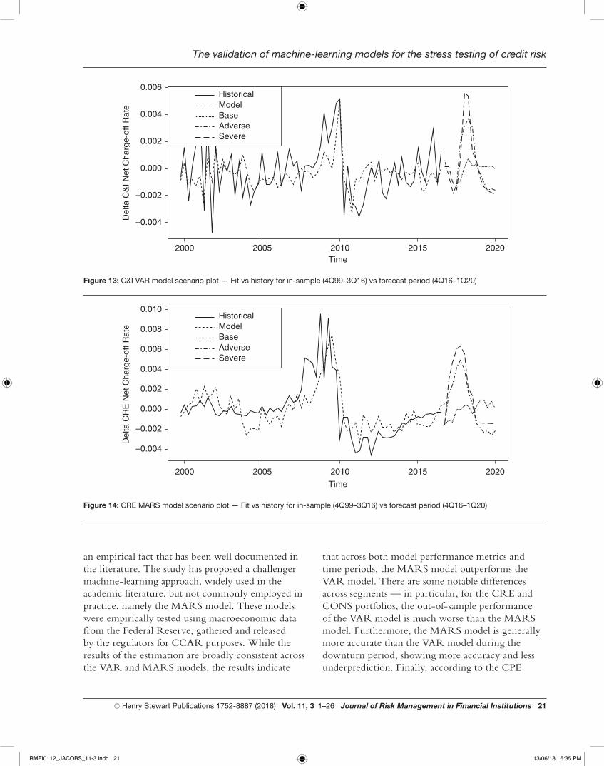
measure of model accuracy — one preferred by regulators — the MARS model performs better by several orders of magnitude. Furthermore, the study finds that the MARS model produces more reasonable forecasts, from the perspective of quality and conservatism in severe scenarios. Across modelling segments, one can observe that the MARS model exhibits greater separation in cumulative loss between base and either adverse or severe scenarios. Furthermore, while the base scenarios are lower in the MARS model compared

with in the VAR model, the adverse and severe scenarios in the former model have much higher cumulative losses than in the latter model.

There are several directions in which this line of research could be extended, including, but not limited to, the following:

• more granular classes of credit-risk models, such as ratings migration or probability-of-default/loss-given-default scorecard/regression;

2005 2010Time

202020152000

–0.005

0.000

Del

ta C

RE

Net

Cha

rge-

off R

ate

0.005

0.010 ModelBaseAdverseSevere

Historical

Figure 15: CRE VAR model scenario plot — Fit vs history for in-sample (4Q99–3Q16) vs forecast period (4Q16–1Q20)

2005 2010Time

202020152000

–0.010

–0.005

Del

ta C

ON

S N

et C

harg

e-of

f Rat

e

0.000

0.005ModelBaseAdverseSevere

Historical

Figure 16: CONS MARS model scenario plot — Fit vs history for in-sample (4Q99–3Q16) vs forecast period (4Q16–1Q20)




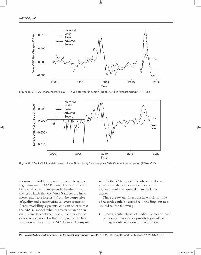
Figure 17: CONS VAR model scenario plot — Fit vs history for in-sample (4Q99–3Q16) vs forecast period (4Q16–1Q20)

• alternative data sets, such as bank or loan-level data; and

• applications related to stress testing, such as regulatory capital or economic capital.

Finally, it is worth noting an important policy implication stemming from this research. When supervisors are evaluating the models employed by banks, there should be an expectation that banks have considered challenger models from different model classes, in particular methodologies with the potential to improve on model accuracy. Conversely, supervisors should also be aware when challenger models have excessive complexity, which would make them difficult to explain or prone to overfitting. What this paper has done with the MARS challenger is to consider something rather different from VAR, while avoiding the more complex machine-learning models, thereby striking the delicate balance between the challenger being fundamentally different but still broadly comparable.

AUTHOR’S NOTEThe model estimation diagnostic plots are available upon request. Note that all residuals exhibit Gaussian behaviour, and in the case of the VAR models, zero autocorrelation, which indicates that the models are well specified.

2005 2010Time

202020152000

–0.010

–0.005

Del

ta C

ON

Net

Cha

rge-

off R

ate

0.005

0.010

0.000

ModelBaseAdverseSevere

Historical

The views expressed in this paper are solely those of the author and do not necessarily represent a view taken by PNC Bank.

References1 Acharya, V. V. and Schnabl, P. (2009) ‘How

banks played the leverage game’, in Acharya, V.V. and Richardson M. (eds), ‘Restoring Financial Stability’, Wiley Finance, New York, NY, pp. 44–78.

2 Demirguc-Kunt, A., Detragiache, E. and Merrouche, O. (2010) ‘Bank capital: lessons from the financial crisis’, World Bank Policy Research Working Paper No. 5473, available at: https://openknowledge.worldbank.org/handle/10986/3955 (accessed 4th June, 2018).

3 Merton, R. (1974) ‘On the pricing of corporate debt: the risk structure of interest rates’, Journal of Finance, Vol. 29, No. 2, pp. 449–470.

4 Board of Governors of the Federal Reserve System (2011) ‘Supervisory Guidance on Model Risk Management’, Supervisory Letter 11-7, Washington, DC, 4th April, available at: https://www.federalreserve.gov/supervisionreg/srletters/sr1107.htm (accessed 4th June, 2018).

5 Basel Committee on Banking Supervision (BCBS) (1988) ‘Internal Convergence of Capital Measurement and Capital Standards: A Revised Framework’, Bank for International Settlements,


https://openknowledge.worldbank.org/handle/10986/3955

https://openknowledge.worldbank.org/handle/10986/3955

https://www.federalreserve.gov/supervisionreg/srletters/sr1107.htm



Jacobs, Jr.


Basel, available at: https://www.bis.org/publ/bcbs04a.htm (accessed 4th June, 2018).

6 Basel Committee on Banking Supervision (1996) ‘Amendment to the Capital Accord to Incorporate Market Risks’, Bank for International Settlements, Basel, available at: https://www.bis.org/publ/bcbs24.htm (accessed 4th June, 2018).

7 Basel Committee on Banking Supervision Committee on Global Financial Systems (2000) ‘Stress Testing by Large Financial Institutions: Current Practice and Aggregation Issues’, April, Bank for International Settlements, Basel, available at: https://www.bis.org/publ/cgfs14.htm (accessed 4th June, 2018).

8 Basel Committee on Banking Supervision (2006) ‘International Convergence of Capital Measurement and Capital Standards: A Revised Framework’, Bank for International Settlements, Basel, available at: https://www.bis.org/publ/bcbs128.htm (accessed 4th June, 2018).

9 Basel Committee on Banking Supervision (2009) ‘Principles for Sound Stress Testing Practices and Supervision’, Consultative Paper No. 155, Bank for International Settlements, Basel, available at: https://www.bis.org/publ/bcbs155.htm (accessed 4th June, 2018).

10 Basel Committee on Banking Supervision (2009) ‘Guidelines for Computing Capital for Incremental Risk in the Trading Book’, Bank for International Settlements, Basel, available at: https://www.bis.org/publ/bcbs159.htm (accessed 4th June, 2018).

11 Basel Committee on Banking Supervision (2009) ‘Revisions to the Basel II Market Risk Framework’, Bank for International Settlements, Basel, available at: https://www.bis.org/publ/bcbs193.htm (accessed 4th June, 2018).

12 Basel Committee on Banking Supervision (2009) ‘Analysis of the Trading Book Quantitative Impact Study’, Bank for International Settlements, Basel, available at: https://www.bis.org/publ/bcbs163.htm (accessed 4th June, 2018).

13 Basel Committee on Banking Supervision (2009) ‘Strengthening the Resilience of the Banking Sector. Consultative Document’, Bank for International Settlements, Basel, available at: https://www.bis.org/publ/bcbs164.htm (accessed 4th June, 2018).

14 Basel Committee on Banking Supervision. (2010) ‘Basel III: A Global Regulatory Framework for More Resilient Banks and Banking Systems’, Bank for International Settlements, Basel, available at: https://www.bis.org/publ/bcbs189.htm (accessed 4th June, 2018).

15 Basel Committee on Banking Supervision (2010) ‘Basel III: An Assessment of the Long-Term Economic Impact of Stronger Capital and Liquidity Requirements’, Bank for International Settlements, Basel, available at: https://www.bis.org/publ/bcbs173.htm (accessed 4th June, 2018).

16 Schuermann, T. (2014) ‘Stress testing banks’, International Journal of Forecasting, Vol. 30, No. 3, pp. 717–728.

17 J.P. Morgan (1996) ‘RiskMetricsTM’ (4th edn), J.P. Morgan, New York, NY.

18 Jorion, P. (1996) ‘Risk2: measuring the value at risk’, Financial Analyst Journal, Vol. 52, No.6, pp. 47–56.

19 Kupiec, P. (1999) ‘Risk capital and VAR’, Journal of Derivatives, Vol. 7, No. 2, pp. 41–52.

20 Berkowitz, J. and Jeremy, A. (1999) ‘Coherent framework for stress-testing’, US Board of Governors of the Federal Reserve System Working Paper No. 99-29, available at: https://ideas.repec.org/p/fip/fedgfe/1999-29.html (accessed 4th June, 2018).

21 Mosser, P.C., Fender, I. and Gibson, M.S. (2001) ‘An international survey of stress tests’, Current Issues in Economics and Finance, Vol. 7, No. 10, pp. 1–6.

22 J.P. Morgan (1997) ‘CreditMetricsTM’ (1st edn), J.P. Morgan, New York, NY.

23 Wilde, T. (1997) ‘CreditRisk+: A Credit Risk Management Framework’, Credit Suisse First Boston, London.

24 Koyluoglu, H, and Hickman, A. (1998) ‘Reconcilable differences’, Risk, October, pp. 56–62.

25 Bangia, A. Diebold, F.X., Kronimus A., Schagen, C. and Schuermann, T. (2002) ‘Ratings migration and the business cycle, with application to credit portfolio stress testing’, Journal of Banking and Finance, Vol. 26, No. 2, pp. 445–474.

26 Board of Governors of the Federal Reserve System (1996) ‘Joint Policy Statement on Interest


https://www.bis.org/publ/bcbs04a.htm

https://www.bis.org/publ/bcbs04a.htm

https://www.bis.org/publ/bcbs24.htm


https://www.bis.org/publ/cgfs14.htm

https://www.bis.org/publ/cgfs14.htm














https://ideas.repec.org/p/fip/fedgfe/1999-29.html

https://ideas.repec.org/p/fip/fedgfe/1999-29.html



Rate Risk (Supervisory Letter 96-13)’, Board of Governors of the Federal Reserve System, Washington, DC.

27 Board of Governors of the Federal Reserve System (1999) ‘Supervisory Guidance Regarding Counterparty Credit Risk Management (Supervisory Letter 99-03)’, Board of Governors of the Federal Reserve System, Washington, DC.

28 Board of Governors of the Federal Reserve System (2002) ‘Interagency Guidance on Country Risk Management (Supervisory Letter 02-05), Board of Governors of the Federal Reserve System, Washington, DC.

29 Foglia, A. (2009) ‘Stress testing credit risk: a survey of authorities’ approaches’, International Journal of Central Banking, Vol. 5, No. 3, pp. 9–37.

30 Inanoglu, H. and Jacobs, Jr., M. (2009) ‘Models for risk aggregation and sensitivity analysis: an application to bank economic capital’, Journal of Risk and Financial Management, Vol. 2, No. 1, pp. 118–189.

31 Jacobs, Jr., M. (2010) ‘Validation of economic capital models: state of the practice, supervisory expectations and results from a bank study’, Journal of Risk Management in Financial Institutions, Vol. 3, No. 4, pp. 334–365.

32 Jacobs, Jr., M. (2013) ‘Stress testing credit risk portfolios’, Journal of Financial Transformation, Vol. 37, pp. 53–75.

33 Rebonato, R. (2010) ‘Coherent Stress Testing: A Bayesian Approach’,Wiley, New York, NY.

34 Jacobs, Jr., M., Karagozoglu, A.K. and Sensenbrenner, F.J. (2015) ‘Stress testing and model validation: application of the Bayesian approach to a credit risk portfolio’, Journal of Risk Model Validation, Vol. 9, No. 3, pp. 1–70.

35 Jacobs, Jr., M. (2015) ‘The impact of asset price bubbles on credit risk measures’, Journal of Financial Risk Management, Vol. 4, No. 4, pp. 251–266.

36 Jacobs, Jr., M. (2017) ‘Asset price bubbles and the quantification of credit risk capital with sensitivity analysis, empirical implementation and an application to stress testing’, Journal of Risk Model Validation, Vol. 11, No. 4, pp. 1–35.

37 Bellman, R. (1957) ‘Dynamic Programming’, Princeton University Press, Princeton, NJ.

38 Wallis, G. and Rolls, E. (1997) ‘Invariant face and object recognition in the visual system’, Progress in Neurobiology, Vol. 51, No. 2, pp. 167–194.

39 Lee, T. and Mumford, D. (2003) ‘Hierarchical Bayesian inference in the visual cortex’, Journal of the Optical Society of America, Vol. 20, No. 7, pp. 1434–1448.

40 Duda, R., Hart, P. and Stork, D. (2000) ‘Pattern Recognition’ (2nd edn), Wiley-Interscience, New York, NY.

41 Itamar, A, Rose, D.C. and Karnowski, T.P. (2010) ‘Deep machine learning-a new frontier in artificial intelligence research [research frontier]’, IEEE Computational Intelligence Magazine, Vol. 5, No. 4, pp. 13–18.

42 Bucheli, H. and Thompson, W. (2014) ‘Statistics and machine learning at scale: new technologies apply machine learning to big data’, paper presented at the SAS Institute Analytics Conference, New York, NY, 14th June.

43 Jones, T. (2017) ‘A Beginner’s Guide to Artificial Intelligence, Machine Learning, and Cognitive Computing’, IBM, New York, NY.

44 Jacobs, Jr., M, Kazmi, S., Klein, L. and Regan, S. (2018) ‘Emerging Trends in the Validation of Machine Learning and Artificial Intelligence Models’, Accenture Consulting, New York, NY.

45 Stock, J.H. and Watson, M.W. (2001) ‘Vector autoregressions’, Journal of Economic Perspectives, Vol. 15, No. 4, pp. 101–115.

46 Sims, C.A. (1980) ‘Macroeconomics and reality’, Econometrica, Vol. 48, No. 1, pp. 1–48.

47 Box, G. and Jenkins, G. (1970) ‘Times Series Analysis: Forecasting and Control’, Holden-Day, San Francisco, CA.

48 Brockwell, P.J. and Davis, R.A. (1991) ‘Time Series: Theory and Methods’, Springer-Verlag, New York, NY.

49 Hanan, E.J. (1971) ‘The identification problem for equation systems with moving average errors’, Econometrica, Vol. 39, No. 1, pp. 751–766.

50 Kohn, R. (1979) ‘Asymptotic results for ARMAX structures’, Econometrica, Vol. 47, No. 1, pp. 1295–1304.


Jacobs, Jr.


51 Hanan, E.J. (1988) ‘The Statistical Theory of Linear Systems’, John Wiley, New York, NY.

52 Commandeur, J.J.F. and Koopman, S.J. (2007) ‘Introduction to State Space Time Series Analysis’, Oxford University Press, New York, NY.

53 R Development Core Team (2018) ‘R: A

Language and Environment for Statistical Computing’, R Foundation for Statistical Computing, Vienna.

54 Friedman, J.H. (1991) ‘Multivariate adaptive regression splines’, Annals of Statistics, Vol. 19, No. 1, pp. 1–67.


Documents

The validation of machine-learning models for the stress