The Validity of Technical Analysis for the Swedish Stock Exchange

The Validity of Technical Analysis for

the Swedish Stock Exchange Evidence from random walk tests and back testing analysis

Master Thesis in Economics

Author: Dan Gustafsson

Tutor: Per-Olof Bjuggren, Louise Nordström Jönköping May 2012

i

Abstract

In this paper I examine the validity of technical analysis for the Swedish stock index

OMXS30 between 2001-12-28 and 2011-12-30. Results indicate that OMXS30 followed a

non-random walk and that technical trading rules had predictive power over future price

movements. Results also suggest that technical trading rules could be used to outperform a

buy-and-hold strategy.

ii

Table of Contents

Abstract ........................................................................................... i

1 Introduction ............................................................................... 1

1.1 Background and Problem Discussion ..................................................... 1 1.2 Previous Research ................................................................................. 2 1.2 Method ................................................................................................... 3

2 Theoretical framework .............................................................. 3

2.1 The Random Walk Theory ...................................................................... 3 2.2 The Efficient Market Hypothesis ............................................................. 4 2.3 Behavioural Finance ............................................................................... 5

2.4 The Dow Theory ..................................................................................... 6 2.5 Technical analysis .................................................................................. 7

3 Research method ...................................................................... 8

3.1 Random Walk Tests ............................................................................... 8 3.1.2 The Box-Pierce Q-test ........................................................................ 8

3.1.3 Lo & MacKinlay’s Variance Ratio Test ............................................... 9 3.2 Trading Rules ....................................................................................... 10 3.2.1 Standard Moving Average ................................................................ 11 3.2.2 Exponential Moving Average ............................................................ 11

3.2.3 The Relative Strength Index ............................................................. 12 3.2.4 RSIstoch ........................................................................................... 12

3.3 Data Selection ...................................................................................... 13

4 Empirical Results .................................................................... 13

4.1 Empirical Results for the Random Walk Tests ..................................... 13 4.2 Empirical Results from Technical Trading Rules .................................. 16

4.3 Empirical Results for Different Investment Strategies ........................... 19

5 Summary and Conclusion ...................................................... 22

References ................................................................................... 23

Appendix ...................................................................................... 26

1

1 Introduction

In the course of years, literally thousands of research papers have tried to appraise the state

of the stock market. In fact, during the past ten decades, few other topics have been so ex-

haustively studied. The rewards to those who are able to anticipate the market are enor-

mous - no wonder the field has attracted so many financial economist and practitioners.

The intensive research has all tried to answer the investor’s problem of how to behave in

the stock market. As a result, two rather different disciplines have arisen. The first disci-

pline is commonly referred to as fundamental analysis and the second discipline as tech-

nical analysis. Fundamental analysis tries to find the “correct” value of a security and, as the

name implies, looks at economic fundamentals to do so. Technical analysis on the other

hand, appraises securities with the use of historical price information.

In this paper I will examine the validity of technical analysis for the Swedish stock index

OMXS30 and see if a strategy based on technical trading rules could have outperform a

buy-and-hold strategy. As such, this paper will be an interesting contribution to the general

discussion of market efficiency, behavioral finance and technical analysis.

1.1 Background and Problem Discussion

At a first glance, the use of technical analysis is quite appealing. The primary reason is the

anticipation to time and beat the market (buy low and sell high) and spend an inordinate

amount of time and research doing so. An investor would no longer need to depend on

profit-loss-statements, auditor’s reports and dividend records. Instead, all an investor need

is historical price data and a trading rule which generates buy and sell signals. However,

finding a trading rule that generates profitable buy and sell signals is easier said than done.

As such, to avoid being whipsawed by seemingly erratic market price movements, an inves-

tor should first and foremost try to understand the fundamental condition of the stock

market before applying technical analysis. For example, if stock markets follow a random

walk, market timing would be impossible using technical analysis. As such, a long term in-

vestment strategy based on the assumption that stock markets generate good rewards in the

long run (from now on called the buy-and-hold strategy), would be superior to any strategy

based on technical trading rules. If price movements are predictable, on the other hand,

technical analysis should be the obvious choice for any investor when appraising securities.

Previous studies have lent some support to the idea that technical analysis could be used to

outperform a buy-and-hold strategy for the Swedish stock exchange (SSE). For example,

both Frennberg and Hansson (1992) and Säfvenblad (2000) rejected the random walk hy-

pothesis (the first obstacle for technical analysis) for the SSE, finding high levels of auto-

correlation. Säfvenblad (2000) suggested that the underlying reason for the SSE’s non-

random walk behavior was negative feedback trading1 (where investors sell after price in-

1 Feedback trading is a form of trading strategy including: profit taking, herding and dynamic asset allocation

(Säfvenblad, 2000)

2

creases). An additional study supporting the use of technical analysis for the SSE is

Metghalchi, Chang and Marcucci (2005). Findings suggested that simple moving average

techniques have had predictive power over future price movements and could outperform

a buy-and-hold strategy for the Swedish stock index OMXS30 between 1986 and 2004.

However, except for Metghalchi et al (2005), the validity of technical analysis for the SSE

has been notably unexamined until now. Furthermore, as Metghalchi et al findings were

based on stock market data between 1986 and 2004, I believe it is high time for a revisit. As

such, I will in this paper examine the validity of technical analysis for the Swedish stock in-

dex OMXS30 and see if a strategy based on technical trading rules could have outperform a

buy-and-hold strategy. To do this I will test the following hypotheses: (1) OMXS30 fol-

lowed a non-random walk, (2) technical trading rules did have predictive power over future

price movements and (3) strategies based on technical trading could outperform a buy-and-

hold strategy.

1.2 Previous Research

Criticism of technical analysis often derives from academic research supporting the “weak

form” efficient market hypothesis as defined by Fama (1970). Specifically, the validity of

technical analysis is often dismissed due to the belief that stock markets follow a random

walk. Examples of studies supporting the random walk hypothesis are: Fama (1965)2, Fama

& Blume (1966)3 and Jensen & Benington (1970)4. However, numerous of research papers

have challenged the random walk hypothesis. In addition to Frennberg & Hansson (1992)

and Säfvenblad (2000), empirical evidence supporting non-random walk behavior for stock

markets are: Lo and MacKinlay (1988)5, Berglund & Liljeblom (1988)6, Chan (1993)7 and

Lima & Tabak (2006)8.

2 Fama (1965) examined stock price movements of the Dow Jones Index between 1956 and 1962. Findings

suggested that price changes were uncorrelated over time and therefore consistent with the random walk hypothesis.

3 Fama & Blume (1966) applied Alexander’s filter technique on closing prices of individual securities of the Dow Jones Index between 1956 and 1962. Fama & Blume concluded that the random walk theory was ad-equate for the average investor due to low serial dependence.

4 Jensen & Benington (1970) reexamined Levy’s trading rules for the NYSE between 1931 and 1965. Findings suggested that Levy’s trading rules were outperformed by a buy-and-hold strategy and that price move-ments had followed a random walk.

5 Lo & MacKinlay (1988) tested the random walk hypothesis by comparing variance estimators for the CRSP return index between 1962 and 1985.Findings strongly rejected the random walk hypothesis.

6 Berglund and Liljeblom (1988) examined the Helsinki stock exchange between 1977 and 1982. Findings suggested first order autocorrelation in index returns due to trading procedures.

7 Chan (1993) examined the smallest and the largest NYSE deciles between 1980 and 1989. Results indicated serial correlation in stock returns.

8 Lima & Tabak (2006) tested the random walk hypothesis for China, Hong Kong and Singapore. Findings rejected the random walk hypothesis for the Singapore stock exchange and B shares for the Chinese stock exchange. Findings supported however the random walk hypothesis for the Hong Kong stock exchange.

3

From the viewpoint of investment strategies, non-random walk behavior can sometimes be

exploited to earn excess returns. As a result, financial economists have tried to find ways to

“beat” the market using technical analysis. In addition to Metghalchi et al (2005), Brock,

Lakonishok & LeBaron (1992) suggested that simple moving average techniques have had

predictive power when examining the Dow Jones Index between 1897 and 1985. Similar

results were found by Bessembinder & Chan (1998) and Craig & Parbery (2005). However,

both Bessembinder et al (1998) and Craig & Parbery (2005) suggested that although mov-

ing average techniques had some predictive power, a buy-and-hold strategy was still superi-

or due to the cost of trade. Kwon & Kish (2002), on the other hand, suggested that tech-

nical trading rules had the possibility to be more profitable than a buy-and-hold strategy

when examining the NYSE.

1.2 Method

The method in this paper is divided into three parts. As technical analysis asserts that suc-

cessive returns are dependent, the first part will establish statistical evidence whether or not

the random walk hypothesis held for OMXS30 between 2001-12-28 and 2011-12-30.

The second part will test whether or not technical trading rules were able to predict future

price movements. In other words, the second part will examine whether or not average dai-

ly buy-day returns from technical trading were significantly (and positively) larger than av-

erage daily sell-day returns. Different trading rules will be tested thru back testing analysis.

The third part will examine what trading strategies, if any, could have been adopted to out-

perform a buy-and-hold strategy.

The theoretical framework will be based on academic research related to technical analysis.

Analysis and conclusion will be based on empirical results and compared to economic the-

ory and previous research.

2 Theoretical framework

This chapter aims to provide a deeper understanding of the financial theory related to technical analysis. Part 2.1 and

2.2 focus on two theories that contest the validity of technical analysis: the random walk theory and the efficient mar-

ket hypothesis. Part 2.3 to 2.5 focus on behaviour economics, the Dow Theory and technical analysis.

2.1 The Random Walk Theory

The random walk theory builds upon a mathematical process were price patterns of finan-

cial markets have no memory and are therefore random. This implies that price changes are

independent from each other and cannot be predicted. The basic premise is that price

movements appear random since they are affected by news and news is always unpredicta-

ble. Originally examined by Maurice Kendall (1953), the concept that financial markets fol-

4

low a random walk gained popularity when Malkiel (1973) compared price movements in

financial markets to a “drunkard’s unsteady gait”.

Cambell, Lo & MacKinlay (1999) define three different versions of the random walk hy-

pothesis. The Random Walk 1 (RW1) model states that all error terms are independent

and identically distributed. Hence, past price patterns includes absolutely no information

about future price changes. RW1 is considered the strongest form of the random walk the-

ory and will be tested with Lo and MacKinlay’s variance ratio test.

The Random Walk 2 (RW2) model states that the distribution of new information, alt-

hough independent, can change over time. The underlying theory of the RW2 model is that

it is not plausible for security prices to have identically distributed increments over a long

time horizon (Cambell, Lo & MacKinlay, 1999).

The Random Walk 3 (RW3) model states that the error terms are uncorrelated. This is to

be considered the weakest form of the random walk hypothesis and is often the one tested

by financial economists through different serial correlation tests. RW3 is considered the

weakest form of the random walk theory since although a trajectory has uncorrelated in-

crements, it could still exhibit dependence if the squared increments are correlated (Cam-

bell, Lo & MacKinlay, 1999). RW3 will be tested with the Box-Pierce Q-test

From an investor’s point of view, the random walk theory is especially interesting since it

contest price predictability. As such, if stock markets follow a random walk, investors can-

not use historical prices to establish profitable trading strategies. Hence, the use of tech-

nical analysis is futile.

2.2 The Efficient Market Hypothesis

First introduced by Fama (1970), the efficient market hypothesis (EMH) builds upon the

assumption that changes in security prices are randomly distributed (follow a random

walk). According to Fama (1970), these random price movements are due to the markets

incorporation of new information. As new information about companies, industries etc. ar-

rives randomly, market reactions should also be random. As such, the EMH do not only

assert that financial markets are informationally efficient but also contest the validity of

technical analysis. Fama (1970) defines three forms of market efficiency.

The weak form market efficiency assumes that all information contained in historical prices

is fully reflected into current prices. While fundamental analysis can be used to outperform

the market, technical analysis will not be able to produce excess returns.

The semi-strong form market efficiency assumes that all public information is fully reflect-

ed into current prices. Investors with information monopoly (insiders) are able to outper-

form the market. However, neither fundamental analysis nor technical analysis will work.

5

The strong form market efficiency assumes that all information, public or private, is fully

reflected into current prices. If strong form market efficiency holds, no single investor can

outperform the market. As such, investors should follow a buy-and-hold strategy.

Empirical evidence in regard to the EMH has been mixed. In fact, after almost four dec-

ades, financial economists and practitioners have not yet reached a consensus as to whether

the EMH holds true for most financial markets. One field that challenge the EMH is be-

haviour finance.

2.3 Behavioural Finance

In contradiction to the EMH that assumes that investors behave with extreme rationality,

behaviour economists suggest that financial markets are full of imperfections in the form

of psychological biases (Barberis, Shleifer & Vishny, 1998). Specifically, behaviour finance

contest the EMH thru commonly observed patterns of choice. Some of the behavioural bi-

ases assumed exhibited in financial markets are explained by prospect theory and regret

theory.

The prospect theory (Kahneman & Tversky, 1979) is considered one of the cornerstones in

behaviour finance. The prospect theory is primarily concerned with how people make

choices that involves risk but where the probabilities of outcomes are known. In contradic-

tion to the expected utility theory9, the prospect theory argues that individuals value losses

more than they value gains. Hence, when comparing losses against gains with the same

probability, losses tend to dominate. In other words, the prospect theory suggests that in-

dividuals are very concerned with small losses. Furthermore, Kahneman et al (1979) sug-

gest that individuals tend to distort probabilities by preferring certainty over uncertainty.

To be more specific, individuals tend to choose prospects with assured outcomes over pro-

spect with uncertain outcomes - even if they offer lower expected utility.

Related to the prospect theory is the regret theory. The regret theory describes how indi-

viduals tend to distort probabilities by making decisions based on anticipated feelings of

regret (Loomes & Sugden, 1982). By making decisions based on anticipatory regrets, indi-

viduals can become either more risk averse or risk loving. That is, some individuals may

avoid making an investments if anticipating regret if the value of the investment declines.

Other individuals may take on investments based on anticipated regret from missing out on

an opportunity. Applied on financial markets, the regret theory can be observed when in-

vestors hold on to loosing investments while locking in gains by selling winners (Odean

1998). This strategy is also known as profit taking and is a form of negative feedback trad-

ing. In markets that exhibit profit taking, investors should expect price reversals after peri-

ods of strong positive gains as investors sell of winning securities.

9 The expected utility theory states that individuals will chose between risky prospects by comparing expected

utility values. In other words, individuals will value prospects by multiplying expected utility with the re-spective probability and chose the prospect generating the highest weighted value (Barbera, Hammond & Seidl, 2004).

6

2.4 The Dow Theory

First introduces by Charles H. Dow, the theory consists of six basic tenants. The first ten-

ant is that markets have three movements: a primary movement, a secondary movement

and a minor movement. The primary movement can last for less than a year and may con-

tinue for several years. The secondary movement are corrections of the primary movement

and normally last for a couple of weeks to a couple of months. In turn, the minor move-

ment are corrections of the secondary movement. These are brief fluctuations and may last

for three weeks (Edwards & Magee, 1997).

The second tenant is that market trends have three phases: an accumulation phase, a distri-

bution phase and a public participation phase. The accumulation phase occurs in bull mar-

kets when astute investors accumulate shares from discouraged sellers. The distribution

phase occurs in bear markets when astute investors sell holdings to optimistic buyers. Trad-

ing activity in the accumulation phase and the distribution phase is however only moderate.

The public participation phase occurs when the public catches on these farsighted inves-

tors. During the public participation phase trading become much more active until the

market boils with activity. At this point, astute investors will initiate a new accumulation or

distribution phase (Edwards & Magee, 1997).

The third tenant is that markets discount all available news (Edwards & Magee, 1997). On

this point, Dow Theory agrees with the efficient market hypothesis.

The fourth tenant is that market averages must confirm one another. In other words, for a

market to fall or rise, related markets must follow. As such, the stock market should not

rise, according to Dow Theory, if positively correlated markets do not rise (Edwards &

Magee, 1997).

The fifth tenant is that volume goes with the trend. This tenant is somewhat related to ten-

ant 2 and states that: as a trend continues, trading activity will expand. The tendency that

volume goes with the trend is mainly concerned with primary market movements but

sometimes hold for secondary market movements as well (Edwards & Magee, 1997).

The sixth tenant is that trends continue until its reversal has been clearly signaled. This ten-

ant is often cited as a warning not to change market positions “too soon”. The tenant

states that odds are in favor of those investors who wait for clear trend reversals, against

investors “jumping the gun”. Essentially, Dow Theory suggests that once a trend has been

clearly established it is very probable that it will continue. However, as the trend progress,

the odds that it will continue grow smaller (Edwards & Magee, 1997).

The validity of Dow Theory has been disputed. Cowles (1933) for example provides evi-

dence against the Dow Theory’s ability to forecast the stock market. Nevertheless the Dow

Theory is considered to be the “granddad” of all technical analysis. Although technical

analysis has developed and now use more sophisticated methods, the basic premises of

Dow Theory lives on.

7

2.5 Technical analysis

Technical analysis is the study of price behavior and aims to predict future price move-

ments on the basis of historical price patterns. The basic premise of technical analysis is

that price movements incorporate human behavior and that human behavior is fairly con-

sistent over time. In other words, due to the irrational nature of the human psychology

(Baumeister & Bushman, 2011), financial markets will be driven by repeated irrational fac-

tors. Thus, technical analysis is not purely technical, as the Dow Theory, but has a very

close link to behavior finance.

Advocates of technical analysis claim that there is a wide divergence between presumed

value and actual price (Edwards & Magee, 1997). I.e. technical traders assume that market

values do not only reflect fundamental statistics but also different value opinions based on

rational and irrational behavior. As such, the only way to find out the true value of a stock

is to observe the characteristics of supply and demand as buyers and sellers trade with each

other. The assumption that markets follow irrational behavior and a supply-demand bal-

ance would be of little interest however, were it not for the three basic principles of tech-

nical analysis, all of which are commonly observed in stock markets (Edwards & Magee,

1997).

Essentially, the three principals of technical analysis are directly related to tenant 1, 2 and 5

of the Dow Theory. The first principle is that financial markets follow trends. Hence, a

large part of technical analysis is to analyze, recognize and exploit assumed trends. As ad-

vocates of technical analysis assume that markets follow irrational behavior and pursue a

supply-demand balance, different trends will occur due to changing price responses to-

wards the market. As price responses are assumed to be composed of two phases: an ac-

cumulation or distribution phase and a public participation phase, trends are assumed to be

fairly consistent. Hence, the second principle of technical analysis is that trends persist. The

third principle is that volume follows the trend. As such, in a bull market, there should be

an increase in volume as the price level goes up. A mirror image occurs for a bear market.

There is however no universal trading rules that can be applied on all financial markets. In

fact, as mentioned above, technical analysis is only useful if the stock markets exhibit non-

random walk behavior. Moreover, even between financial markets that exhibit a non-

random walk, trading results based on the same trading rules may differ. Investors should

therefore be careful and evaluate the fundamental condition of the stock market before ap-

plying technical analysis.

8

3 Research method

In this chapter I intend to give a thorough description of the tests and models used to examine the validity of technical

analysis for OMXS30. The chapter is divided into two parts. The first part will concentrate on two random walk

tests: the Box-Pierce Q-test and Lo & MacKinlay’s single variance ratio test. The second part will focus on technical

trading rules related to financial theory and previous studies.

3.1 Random Walk Tests

As technical analysis asserts that successive returns are dependent, I seek evidence support-

ing the first hypothesis: that OMXS30 followed a non-random walk between 2001-12-28

and 2011-12-30. I will evaluate the random walk hypothesis with two random walk tests:

the Box-Pierce Q-tests and Lo & MacKinlay’s single variance ratio tests.

3.1.2 The Box-Pierce Q-test

The Box-Pierce Q-test (Box & Pierce, 1970) is a method to test for serial correlation in a

time series. I will use the Box-Pierce Q-statistic to test the weakest form of the random

walk hypothesis (RW3) with a null hypothesis of no serial correlation. The Q-statistic is a

linear equation of equally weighted squared autocorrelation coefficients and is asymptoti-

cally distributed as the chi-squared distribution. As defined by Box & Pierce (1970) the sta-

tistic is calculated as:

( ) ∑

where n is the sample size, m is the number of autocorrelation coefficient and the vari-

ous squared autocorrelation coefficients. is calculated as:

( ) ∑

∑

The Box-Pierce Q-statistic assumes that the innovations are normally distributed. It

turns out that this assumption is a bit problematic since many stock markets exhibits a lep-

tokurtic distribution. Nonetheless, since the asymptotic normality of the autocorrelation

coefficients does not require that the innovations are normally distributed (Anderson

& Walker, 1964) the Box-Pierce Q-statistic should still be considered a useful tool to detect

serial correlation.

9

3.1.3 Lo & MacKinlay’s Variance Ratio Test

The second random walk test I will employ is Lo & MacKinlay’s (1988) single variance ra-

tio test. As many random walk tests concentrate on testing RW3 (such as the Box-Pierce

Q-test), Lo and MacKinlay’s variance ratio test is used to evaluate the strongest form of the

random walk hypothesis (RW1). Furthermore, variance ratio tests are superior to other

random walk tests when more than 256 observations are regarded (Chow & Denning,

1993). As such, the variance ratio test should provide more meaningful results when analys-

ing the nature of stock market price movements.

The idea behind Lo and MacKinlay’s single variance ratio test is that the increments of the

variance of stock returns should be proportional to the observation interval. For the ran-

dom walk hypothesis to hold, the variance of the increments in the trajectory must be line-

ar. Consider the following equation:

( )

denote the natural logarithm of the price of the stock or index at time t, denote an ar-

bitrary drift parameter and denote the random disturbance term. In order for the random

walk theory to hold, the variance ratio for must be twice as large as the variance

for . Consequently, the random walk theory can be tested using the variance ra-

tio test by comparing and 1/n times (Lo & MacKinlay, 1988). Lo

and MacKinlay show that the variance ratio statistic is equivalent to:

( ) ( ) ( ) ∑ ( )

( )

where q is the observation interval of different variance estimator, ( ) is the j-th order au-

tocorrelation coefficient of the first differences of and ( ) is the unbiased variance

ratio estimator. Since ( ) approaches zero under the null hypothesis that the variance

ratio equals one, only the asymptotic variance of ( ) needs to be computed to perform

the standard inference (Lo & MacKinlay, 1988). Given the variance ratio statistic, the null

hypothesis of equal variances can be defined as:

( )

Following Lo & MacKinlay (1988) I will use two different test statistics: The first test statis-

tic in the case of homoscedasticity assumes i.i.d. error terms and is calculated as:

( ) ( ) √ ( ( ))

√ ( )

where ( )is the asymptotic variance of ( ) which can be defined as:

10

( ) ( ) ( )( )

( )

The second test statistic is the robust z-statistic in the case of heteroscedasticity. Since

hetroscedasticity can explain the rejection of the random walk hypothesis (RW1), the ro-

bust test statistic is of great importance. In other words, if the robust z-statistic is signifi-

cant, the rejection of the random walk hypothesis is not due to changing variances because

of heteroscedasticity (time varying variances). The robust test statistic is calculated as:

( ) ( ) √ ( ( ))

√ ( )

where ( ) is the heteroscedasticity-consistent estimator of the asymptotic variance of

( ) which can be defined as:

( ) ( ) ∑[ ( )

]

( )

where ( ) is the heteroscedasticity-consistent estimator of the variance of the autocorrela-

tion coefficient estimator. ( ) is computed as:

( ) ( ) ∑ (

)

( )

[∑ ( ) ]

where is the average return. In this paper, I will use observation intervals (q) of 2, 4, 8

and 16.

3.2 Trading Rules

This section seeks evidence supporting the second hypothesis that technical trading rules

did have predictive power over future price movements of OMXS30 between 2001-12-28

and 2011-12-30. I will assume that OMXS30 follow trends in the primary market move-

ment. I therefore adopt two trend determinants: the standard moving average (SMA) and

the exponential moving average (EMA). Following Säfvenblad’s (2000) findings that

OMXS30 exhibit negative feedback trading, where investors sell after price increases (profit

taking), I also introduce two oscillators: the relative strength index and the RSIstoch. As

these oscillators measures the power of directional price changes, they might be a useful

tool to detect price reversals generated from profit taking behaviour. In addition, I have al-

so followed up on successful trading rules for OMXS30 examined by Metghalchi et al

(2005): the Arnold and Rahfeldht moving average technique and price relative to an SMA.

For brevity, descriptions for the two trading rules are found in the appendix (section 1.1).

11

To evaluate the different trading rules I will use the Welch t-statistic. The Welch t-test is

employed when population variances are assumed to be different and when the sample siz-

es are not equal. A description of the Welch t-statistic is found in the appendix (section

2.2). All trading rules will be tested at the 5% significance level. Furthermore, I will assume

that the index level remains stable during the last few minutes of trading. An investor will

therefore be able to place next day’s market position at the close.

3.2.1 Standard Moving Average

Standard Moving Average (SMA) techniques are some of the most popular trend calcula-

tions (Kaufman, 2003). The main use of the SMA is to smooth out day-to-day fluctuations

in security prices and by that identify assumed trends. The standard moving average takes

the average from past closing prices over a predetermined time period and is calculated as:

( )

∑

is the number of days in the predetermined time period and is the price level. Alt-

hough the 200-day moving average seems to be the benchmark, investors can choose

themselves how long or short the time period should be. There are no specific rules in re-

gard to that. However, while shorter time periods tends to be more responsive to price

changes, longer time periods will provide more reliable estimates on the long-term trend.

In this paper, a “buy-signal” is generated when a short SMA moves above a long SMA.

Likewise, a “sell-signal” is generated when a short SMA moves below a long SMA. The

main reason for using a short SMA instead of the index price level is to avoid being whip-

sawed by erratic price movements.

3.2.2 Exponential Moving Average

While the SMA assign equal weights to past observations, the exponential smoothening ef-

fect incorporated in the exponential moving average (EMA), assign exponentially decreas-

ing weights to past observations over time. Hence, EMA brings the exponential value clos-

er to the last closing price by assigning greater importance to recent data. The starting value

of the EMA is usually the simple moving average for N days. The following values of the

EMA are calculated as:

( ) ( )

is the last known price and the smoothing factor. When assigning the smoothing factor

it is important to remember that while smaller values of tends to produce trend values

more responsive to price changes, larger values of will provide more reliable estimates on

the long-term trend. I will however adopt a more common practice and calculate the

smoothing factor with the following formula:

12

( )

where is the number of observations included in the starting value. The trading rule for

EMA is similar to the trading rule for the SMA. A “buy-signal” is generated when a short

EMA moves above a long EMA. Consequently, a “sell-signal” is generated when a short

EMA moves below a long EMA.

3.2.3 The Relative Strength Index

First introduced by Wells Wilder, the relative strength index (RSI) provides a ratio of the

upward price movement relative to the total price (Kaufman, 2003). To be more specific,

the RSI is a measure of the power of directional price changes. The RSI is computed as:

( )

where is the ratio between average up changes to average down changes. Wilder rec-

ommended the to be calculated over 14 days (Kaufman, 2003). The basic idea behind

the RSI is that a security can be considered “overbought” if the price level moves up very

rapidly. Once a security is considered “overbought” the price is assumed to rebound and

fall. Hence, the RSI can be used to exploit profit taking behavior. Normally, a security is

considered “overbought” when the RSI is above 70 (Murphy 1999).

A common usage of the RSI is to detect potential market entry and exit points once a long

term positive trend has been established (Kirkpatrick & Dahlquist, 2007). As such, the RSI

will not be used as a single indicator. Instead I will use the RSI in combination with SMAs

and EMAs. I will consider the index to be “overbought” when the RSI is above 70. At this

point, I will expect the market to rebound as investors lock in gains from winning stocks

and thereby exit the market.

3.2.4 RSIstoch

The RSIstoch is an extension of the RSI. However, instead of applying the stochastic for-

mula on price movements, RSIstoch applies it on the relative strength index. Developed by

Chande & Kroll (1994) the RSIstoch aims to mitigate problems related to the RSI. Chande

and Kroll argued that the RSI often register below 70 for longer periods but seldom reach

levels of “overbought”. Thus, investors can be left with very few trades based on the RSI if

only following the fundamental tenets. By measuring the level of the RSI relative to its

range over a predefined period, the RSIstoch tries to combat this shortcoming. In other

words, the RSIstoch is a more sensitive measure of the power of directional price changes.

The RSIstoch is calculated as:

( )

13

where is the lowest low for the RSI for the given time period and the highest

high for the RSI for the given time period. Investors can choose themselves how long or

short the time period should be. I will however use the same time period as for the RSI of

14 trading days.

As for the RSI, the RSIstoch will not be used as a single indicator. The RSIstoch will in-

stead be used to detect potential market entry and exit points once a positive trend has

been established using SMAs and EMAs. I will assume that the index will rebound and

thereby exit the market once the RSIstoch is above 0.80.

3.3 Data Selection

I will use closing prices from OMXS30. OMXS30 is an index which involves OMX Stock-

holm’s most traded stocks and should provide a good general picture of the Swedish stock

exchange. Furthermore, using the OMXS30 index I will mitigate biases related to illiquidity.

In other words, an investor should be able to buy and sell shares quickly without seeing a

relevant change in price. The data I will use is taken from NasdaqOMX. The time period I

will examine is between 2001-12-28 and 2011-12-30. I have chosen this time period since it

includes periods of both high and low volatility. In addition, I believe that a time period of

ten years is substantial for examining the topic at hand.

4 Empirical Results

This chapter will be divided into three parts. The first part will summarize empirical results from two random walk

tests. The Box-Pierce Q-test and Lo & MacKinlay’s single variance ratio test. The second part will summarize the

results from different trading rules to assert if technical trading rules could have been used to predict recurring price

patterns. The third part will summarize which trading strategies, if any, could have been adopted to outperform the

buy-and-hold strategy.

4.1 Empirical Results for the Random Walk Tests

This section summarizes the results from two different random walk tests: the Box-Pierce

Q-test and Lo & MacKinlay’s single variance ratio test. I seek evidence rejecting the ran-

dom walk theory for OMXS30.

Table 1 summarize the statistical results from the Box-Pierce Q-test. To test the validity of

the random walk hypothesis (RW3), Q-statistics are calculated for lags 1 – 10. For daily ob-

servations we cannot reject the null hypothesis of no serial correlation at the 5% signifi-

cance level for lag m = 1 and m = 2. However, there is a clear rejection of the null hypoth-

esis of no serial correlation for m = 3 to m = 10. The main source of high autocorrelation

seems to be generated from lag 3. For weekly observations there is a strong rejection of the

null hypothesis of no serial correlation for all lags. The main source of high autocorrelation

14

comes from lag 1. Hence, using the Box Pierce Q-test, both weekly and daily samples reject

the weak-form random walk hypothesis (RW3) at the 5% significance level.

Table 1

Statistical results for the Box-Pierce Q-test

M Q statistic M Q statistic

Panel 1: Daily data

1 1,00250 6 26,1525*

(0.317)

(0.000)

2 2,2756 7 26,2936*

(0,321)

(0.000)

3 17,8339* 8 27,7251*

(0.001)

(0.001)

4 23,8478* 9 27,9557*

(0.000) (0.001)

5 23,8478* 10 29,9458*

(0.000) (0.001)

Panel 2: Weekly data 1 14,5787* 6 27,9422*

(0.000)

(0.000)

2 14,8097* 7 36,7125*

(0.001)

(0.000)

3 17,4523* 8 38,8313*

(0.001)

(0.000)

4 19,9496* 9 40,2186*

(0.001)

(0.000)

5 23,4009* 10 42,2689*

(0.000) (0.000) m correspond to the number of lags, Q is the Box-Pierce Q-statistic. Reported below the Box-Pierce Q-statistic are the corresponding p-values. Numbers marked with asterisks are significant at the 5% significance level.

q correspond to aggregation values, VR is the Variance Ratio, M(q) is the Variance Ratio estimator, N is the number of observations. Reported below the Z-statistics are the corresponding p-values. Numbers marked with asterisks are significant at the 5% significance lev-el.

Table 2

Statistical results for Lo & MacKinlay VR test Q VR M (q) Z Robust Z N

Panel 2: Daily data 2 0,98053 -0,01947 -0,9768 -0,6990 2516

(0.329) (0.485) 4 0,91039 -0,08961 -2,4024* -1,6701 2516

(0.016) (0.095)

8 0,80362 -0,19638 -3,3274* -2,2665* 2512

(0.001) (0.0234)

16 0,75265 -0,24735 -2,8164* -1,9192 2512

(0.005) (0.055)

Panel 1: Weekly data

2 0,00878 -0.12247 -3,7525* -2,3545* 520

(0.000) (0.018)

4 0,81117 -0,18883 -2,3016* -1,5843 520

(0.021) (0.113)

8 0,84475 -0,15525 -1,1968 -0,8725 520

(0.231) (0.383)

16 1,0872 0,018722 0,0962 0,0712 512

(0.923) (0.943)

15

Table 2 shows the statistical results for Lo & MacKinnlay’s variance ratio test. To test the

strong form random walk hypothesis (RW1), z-statistics are calculated for observation in-

tervals of q = 2 to q = 16. For daily observations, I cannot reject the null hypothesis that

VR = 1 for q = 2. However, in the case of homoscedasticity, there is a clear rejection of the

null hypothesis that VR = 1 for q = 4 to q = 16. These findings are validated by the robust

z-statistic (in the case of heteroscedasticity) for the aggregation value of q = 8. For weekly

data, in the case of homoscedasticity, the null hypothesis that VR = 1 is rejected for the ag-

gregation values of q = 2 and q = 4. These findings are validated by the robust z-statistic

for the aggregation value of q = 2. As such, weekly and daily samples do not only reject the

strong-form random walk hypothesis (RW1) but also the hypothesis of weak form efficien-

cy for OMXS30.

Findings are therefore similar to the findings of Frennberg & Hansson (1992) and Säfven-

blad (2000) who found high levels of autocorrelation (although my results contest Säfven-

blads findings of first order serial correlation for daily data). Säfvenblad suggested that the

underlying reason for the high level of autocorrelation was negative feedback trading. If

negative feedback trading is consistent among stocks, a non-random walk should be ob-

served for index returns. However, since Säfvenblad used a different methodology, findings

are only constrictive comparable.

Two important implications follow OMXS30’s non-random walk behavior. The first impli-

cation, which I will concentrate on for the remainder of this paper, is that technical analysis

can (in theory) be used to predict future price movements. In fact, in the case of a non-

random walk, investors should take historical price information into consideration for their

investment decisions. However, for technical analysis to work in reality, return correlations

need to be large enough to cover transaction costs. This will be examined further in section

4.2 and 4.3.

The second implication is that the Swedish stock exchange can become a heaven for specu-

lation10. Since OMXS30 do not follow a random walk, the returns of speculative market

positions are dependent and therefore predictable. Hence, speculators can realize large

gains, given an inordinate amount of risk. Furthermore, in an inefficient market, the moni-

toring of market manipulation is complicated (Otto 2010). Speculators can therefore create

false appearances with respect to the price of securities, deliberately mislead other investors

and potentially worsen market efficiency. As such, the usefulness of fundamental analysis is

reduced and technical analysis will become even more important.

10 Speculation refers to investment strategies which involves taking on large amount of risk in hope for large

gains. Speculation can contribute to making financial markets more efficient due to market exploitation. However, in the presence of speculators, real demand and supply can be distorted and thus prices become misleading.

16

4.2 Empirical Results from Technical Trading Rules

This part will summarize the results from different technical trading rules. Knowing that

OMXS30 did not follow a random walk, I seek evidence that technical analysis could have

been used to predict recurring price patterns.

For comparison, between 2001-12-28 and 2011-12-30, the average daily return for the buy-

and-hold strategy was 0.0184%, the standard deviation 0.016 and the total number of trad-

ing days 2517. Given the average daily return, the standard deviation and the number of

trading days, the t-statistic for the buy-and-hold strategy, using the one sample t-test (see

Appendix, section 2.1), is 0.58

√

Compared with the critical value of 1.96 at the 5% significance level, the average daily re-

turn for the buy-and-hold strategy is not significantly larger than zero. Interestingly, this

implies that a buy-and-hold strategy have not provided positive average daily returns be-

tween 2001-12-28 and 2011-12-30.

Table 6 and 7 (Appendix, section 3) reports trading results based on multiple SMA rules

and multiple EMA rules. The trading rule was to enter the market when the short moving

average moved above the long moving average and exit the market when the short moving

average moved below the long moving average. Findings are not spectacular. Although all

trading rules provide positive average daily returns on buy-days and negative average daily

returns on sell-days, only MA (50-200) is able to generate significant t-statistics for buy-sell

returns. These findings give some support that OMXS30 follow trends. However, return

correlation do not seem to be strong enough to provide strong price predictions.

Table 8 and 9 (Appendix, section 3) show trading results based on multiple SMAs and mul-

tiple EMAs in combination with the RSI. The trading rule was to enter the market when

the short moving average moved above the long moving average while the RSI was below

70. I would exit the market when the short moving average moved below the long moving

average or when the RSI moved above 70. Eight out of the twelve examined trading rules

are able to generate average daily buy-day returns that were significantly larger than average

daily sell-day returns.

Table 10 and 11 (Appendix, section 3), reports trading results based on multiple SMA rules

and multiple EMA rules in combination with the RSIstoch. The trading rule was to enter

the market when the short moving average moved above the long moving average while

the RSIstoch was below 0.80. I would exit the market when the short moving average

moved below the long moving average or when the RSI moved above 0.80. As for the

combination with the RSI, a majority of the trading rules provide average daily buy-day re-

turns that are significantly larger than average daily sell-day returns. As expected, the intro-

duction of the more sensitive RSIstoch generates more trades than the RSI. However, since

the RSI provides higher t-statistics it is possible to consider the RSIstoch as oversensitive

for OMXS30.

17

Interestingly, the introduction of the RSI and the RSIstoch (which indicates the strength of

directional price changes) seems to have an impact on price predictability. It is clear that

OMXS30 exhibit price reversals after periods of positive returns and that these price rever-

sals are exploitable. I view these results as further evidence supporting Säfvenblads (2000)

suggestion that the Swedish stock market exhibit negative feedback trading (which include

profit taking). Something which can also explain OMXS30’s non-random walk behaviour

(Säfveblads, 2000).

Table 12 and 13 (Appendix, section 3) summarize trading results based on price relative to

an SMA and Arnold and Rahfeldt’s moving average technique. In contrast to Metghalchi et

al (2005) findings, none of the trading rules are able to outperform average daily returns of

the buy-and-hold strategy. In addition, none of the strategies are able to provide average

daily buy-day returns significantly larger than average daily sell-day returns. In fact, trading

based on Arnold and Rahfeldt moving average technique provide negative buy-sell t-

statistics. This new failure to predict stock returns for the two trading rules can reflect ei-

ther (1) the market has become efficient or (2) trend patterns has changed. Since both the

random walk tests and technical trading rules support a non-random walk for OMXS30, I

conclude that trend patterns can change over time. This could be a result from changes in

stock market volatility. As changes in stock market volatility can relate to changes in ex-

pected returns (Merton, 1980), trend behaviour might have shifted.

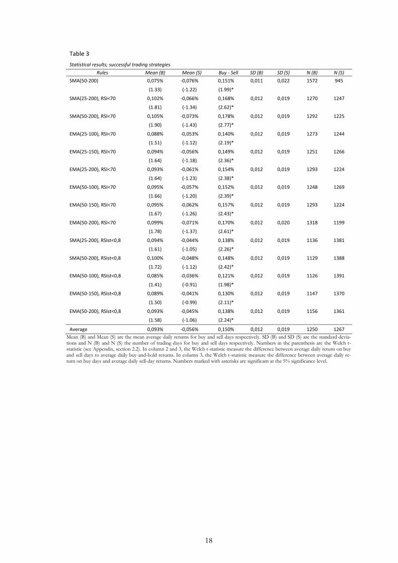
A summary of trading rules with significantly larger average daily buy-day returns than sell-

day returns are reported in table 3. Overall findings lend support to the assumption that

technical analysis can be used to predict future price movements. If technical analysis could

not predict future price movements, average daily buy-day returns would not be significant-

ly larger than average daily sell-day returns. As such, I cannot reject my second null hy-

pothesis that technical trading rules did have predictive power over future price move-

ments. Interestingly, all trading rules reported in table 3 provide negative returns for sell

days. Due to an even weighted number of buy and sell days, this cannot be explained by

seasonal effects (Brock et al, 1992). Instead, the predictability of price movements should

provide further support that OMXS30 follow an exploitable non-random walk. Equally in-

teresting is how all trading rules report higher volatility on sell-days than on buy-days. The-

se findings are consistent with the asymmetric volatility phenomenon which suggests that

volatility tends to be high following negative returns and low following positive returns

(Dufour, Garcia & Taamouti, 2012). Possible explanations for asymmetric volatility are:

leverage effects11 and volatility feedback12 (Bekaert & Wu, 2000). As such, price predictabil-

ity of OMXS30 is not only associated with higher returns but also lower risk.

11The leverage effect occurs when the price of a corporate security falls. As the equity of the firm decreases

the leverage increases. As such, the security will become more risky which increases its price volatility (Bekaert & Wu, 2000).

12The volatility feedback theory assumes that there exist a positive relationship between expected return and volatility. As increased volatility increase expected returns and lower stock prices, good news will cause vol-atility to go down and bad news will cause volatility to go up (Bekaert & Wu, 2000).

18

Table 3

Statistical results; successful trading strategies

Rules Mean (B) Mean (S) Buy - Sell SD (B) SD (S) N (B) N (S)

SMA(50-200) 0,075% -0,076% 0,151% 0,011 0,022 1572 945

(1.33) (-1.22) (1.99)*

SMA(25-200), RSI<70 0,102% -0,066% 0,168% 0,012 0,019 1270 1247

(1.81) (-1.34) (2.62)*

SMA(50-200), RSI<70 0,105% -0,073% 0,178% 0,012 0,019 1292 1225

(1.90) (-1.43) (2.77)*

EMA(25-100), RSI<70 0,088% -0,053% 0,140% 0,012 0,019 1273 1244

(1.51) (-1.12) (2.19)*

EMA(25-150), RSI<70 0,094% -0,056% 0,149% 0,012 0,019 1251 1266

(1.64) (-1.18) (2.36)*

EMA(25-200), RSI<70 0,093% -0,061% 0,154% 0,012 0,019 1293 1224

(1.64) (-1.23) (2.38)*

EMA(50-100), RSI<70 0,095% -0,057% 0,152% 0,012 0,019 1248 1269

(1.66) (-1.20) (2.39)*

EMA(50-150), RSI<70 0,095% -0,062% 0,157% 0,012 0,019 1293 1224

(1.67) (-1.26) (2.43)*

EMA(50-200), RSI<70 0,099% -0,071% 0,170% 0,012 0,020 1318 1199

(1.78) (-1.37) (2.61)*

SMA(25-200), RSIst<0,8 0,094% -0,044% 0,138% 0,012 0,019 1136 1381

(1.61) (-1.05) (2.26)*

SMA(50-200), RSIst<0,8 0,100% -0,048% 0,148% 0,012 0,019 1129 1388

(1.72) (-1.12) (2.42)*

EMA(50-100), RSIst<0,8 0,085% -0,036% 0,121% 0,012 0,019 1126 1391

(1.41) (-0.91) (1.98)*

EMA(50-150), RSIst<0,8 0,089% -0,041% 0,130% 0,012 0,019 1147 1370

(1.50) (-0.99) (2.11)*

EMA(50-200), RSIst<0,8 0,093% -0,045% 0,138% 0,012 0,019 1156 1361

(1.58) (-1.06) (2.24)*

Average 0,093% -0,056% 0,150% 0,012 0,019 1250 1267

Mean (B) and Mean (S) are the mean average daily returns for buy and sell days respectively. SD (B) and SD (S) are the standard devia-tions and N (B) and N (S) the number of trading days for buy and sell days respectively. Numbers in the parenthesis are the Welch t-statistic (see Appendix, section 2.2). In column 2 and 3, the Welch t-statistic measure the difference between average daily return on buy and sell days to average daily buy-and-hold returns. In column 3, the Welch t-statistic measure the difference between average daily re-turn on buy days and average daily sell-day returns. Numbers marked with asterisks are significant at the 5% significance level.

19

4.3 Empirical Results for Different Investment Strategies

Knowing that OMXS30 do not follow a random walk and that technical analysis can be

used to predict recurring price patterns, I will try to adopt a trading strategy that can out-

perform the buy-and-hold strategy. So far, I have only considered a trading strategy were I

am in the market on buy-days and out of the market on sell-days. That will give me average

daily returns for the entire time period based on the following formula:

( ) (

) (

)

where , and is the number of buy-days, sell-days and buy-and-hold days respective-

ly. and are the average daily return for buy-days and sell-days respectively. Since

equals zero and is unable to outperform average daily buy-and-hold returns, it is easy to

conclude that this strategy will not be able to outperform the buy-and-hold strategy. Fol-

lowing Metghalchi et al (2005), I will therefore introduce two different trading strategies.

The first trading strategy (S1) involves being in the stock market on buy days and in the

Swedish money market on sell days. The second strategy (S2), which builds upon my find-

ings of asymmetric volatility, involves borrowing from the money market to double the in-

vestment in the stock market on buy-days while being in the money market on sell-days.

Lending and borrowing returns for the Swedish money market are based on yearly averages

of lending and borrowing rates from the Swedish Riksbank (Appendix: section 4, table 14).

The sample size of S1 and S2 will equal the sample size of the buy-and-hold strategy.

Hence I can no longer use the Welch t-test to evaluate my results. I will instead subtract

daily returns of the buy-and-hold strategy from daily returns of S1 and S2. The difference is

then calculated to find average daily returns and the standard deviation. As such, I can now

use the one-sample t-test (Appendix: section 2.1) to evaluate if the difference between the

buy-and-hold strategy and S1 and S2 is significantly larger than zero. If the difference is

significantly larger than zero I will conclude that the given strategy is able to outperform

the buy-and-hold strategy. However, I must also consider the level of risk. Again, I will

evaluate my results on a 5% significance level.

I will also calculate the break-even trading cost for trading rules that outperform the buy-

and-hold strategy. Many financial institutions request between 0.00% and 0.15% in com-

mission for equity trading with a minimum commission between 9 SEK and 99 SEK (Ap-

pendix: section 5, table 15). As the relative cost for the minimum commission depends on

the invested amount, I will concentrate on the fixed percentage commission and regard the

highest cost of 0.15% as my benchmark. As such, trading rules with break-even transaction

costs below 0.15% will not be regarded superior to the buy-and-hold strategy. I will assume

the same transaction cost for buying and selling.

Table 4 summarizes the results for S1. S1 involves being in the stock market on buy-days

and in the money market on sell-days. Average returns for the different trading rules are

0.032%, average standard deviation 0.014 and average number of trades 185. The break

even trading cost is not reported since none of the trading rules provide average daily re-

20

turns significantly larger than zero. I can therefore conclude that the use of leverage is nec-

essary. In other words, it is necessary to take on higher risk to outperform the buy-and-

hold strategy.

Table 4

Statistical results successful trading rules, Strategy 1

Rules Mean diff SDdiff SD Trades B/E TC Sharpe-ratio

SMA(50-200) 0,032% 0,013 0,009 6 - 0,049

(1.20)

SMA(25-200), RSI<70 0,037% 0,014 0,008 168 - 0,058

(1.35)

SMA(50-200), RSI<70 0,039% 0,014 0,008 166 - 0,061

(1.45)

EMA(25-100), RSI<70 0,029% 0,014 0,008 188 - 0,049

(1.07)

EMA(25-150), RSI<70 0,032% 0,014 0,008 176 - 0,054

(1.19)

EMA(25-200), RSI<70 0,033% 0,014 0,008 178 - 0,054

(1.22)

EMA(50-100), RSI<70 0,033% 0,014 0,008 170 - 0,054

(1.21)

EMA(50-150), RSI<70 0,034% 0,014 0,008 176 - 0,054

(1.25)

EMA(50-200), RSI<70 0,037% 0,014 0,009 176 - 0,058

(1.38)

SMA(25-200), RSIst<0,8 0,029% 0,014 0,008 228 - 0,052

(1.05)

SMA(50-200), RSIst<0,8 0,031% 0,014 0,008 240 - 0,055

(1.16)

EMA(50-100), RSIst<0,8 0,025% 0,014 0,008 228 - 0,046

(0.89)

EMA(50-150), RSIst<0,8 0,027% 0,014 0,008 240 - 0,049

(0.98)

EMA(50-200), RSIst<0,8 0,029% 0,014 0,008 244 - 0,051

(1.06)

Average 0,032% 0,014 0,008 185 - 0,053

Mean diff is the average daily return when average daily buy-and-hold returns are subtracted from S2’s average daily returns. SDdiff is the standard deviation when average daily buy-and-hold returns are subtracted from S2’s average daily returns. SDdiff is used for the t-statistic. SD is the standard deviation for S2. B/E TC is the break-even trading cost for the different trading rules and R is the realized re-turn during the given time period. Numbers marked with asterisks are significant at a 5% significance level.

Table 5 reports the results for S2. S2 involves borrowing at the money market to double

the investments in the stock market on buy days while being in the money market on sell-

days. Average return for the different trading rules is 0,073%, average standard deviation

0,016 and average number of trades 185. All trading rules except the combination of EMA

(50-100) and RSIstoch are able to outperform the buy-and-hold strategy when ignoring

transaction costs. When including transaction costs, 8 out of the 13 trading rules are still

able to outperform the buy-and-hold strategy (break-even costs higher than 0.15%).

Interestingly, the standard deviation for many of the trading rules under S2 are similar to

the standard deviation for the buy-and-hold strategy (average 0.017 for S2 compared to

21

0.016 for the buy-and-hold strategy). As such, even though S2 generates significantly higher

average daily returns, I end up with roughly the same risk as for the buy-and-hold strategy.

Findings that S2 have higher risk adjusted performance than the buy-and-hold strategy are

confirmed by the Sharpe ratios13 for average daily returns (the Sharpe ratio for average daily

buy-and-hold returns is 0.007). These results are consistent with Metghalchi et al (2005)

findings. However, since the two papers use different trading rules, findings are only con-

strictive comparable. As such, I cannot reject my third hypothesis: that technical analysis

could be used to outperform the buy-and-hold strategy. In other words, the use of tech-

nical analysis for the Swedish stock market was fully valid and applicable between 2001-12-

28 and 2011-12-30.

Table 5

Statistical results successful trading rules, Strategy 1

Rules Mean diff SDdiff SD Trades B/E TC Sharpe-ratio

SMA(50-200) 0,074% 0,016 0,018 6 4,447% 0,008

(2.32)

SMA(25-200), RSI<70 0,083% 0,016 0,017 168 0,310% 0,008

(2.60)

SMA(50-200), RSI<70 0,088% 0,016 0,017 166 0,397% 0,008

(2.77)

EMA(25-100), RSI<70 0,067% 0,016 0,017 188 0,068% 0,008

(2.12)

EMA(25-150), RSI<70 0,075% 0,016 0,017 176 0,178% 0,008

(2.34)

EMA(25-200), RSI<70 0,076% 0,016 0,017 178 0,193% 0,008

(2.38)

EMA(50-100), RSI<70 0,076% 0,016 0,017 170 0,201% 0,008

(2.38)

EMA(50-150), RSI<70 0,077% 0,016 0,017 176 0,218% 0,008

(2.43)

EMA(50-200), RSI<70 0,084% 0,016 0,017 176 0,314% 0,008

(2.64)

SMA(25-200), RSIst<0,8 0,067% 0,016 0,016 228 0,055% 0,008

(2.11)

SMA(50-200), RSIst<0,8 0,072% 0,016 0,016 240 0,103% 0,008

(2.26)

EMA(50-100), RSIst<0,8 0,059% 0,016 0,016 228 - 0,008

(1.84)

EMA(50-150), RSIst<0,8 0,063% 0,016 0,016 240 0,009% 0,008

(1.99)

EMA(50-200), RSIst<0,8 0,067% 0,016 0,016 244 0,052% 0,008

(2.12)

Average 0,073% 0,016 0,017 185 0,503% 0,008

Mean Rdiff is the average daily return when average daily buy-and-hold returns are subtracted from S2’s average daily returns. SDdiff is the standard deviation when average daily buy-and-hold returns are subtracted from S2’s average daily returns. SDdiff is used for the t-statistic. SD is the standard deviation for S2. B/E TC is the break-even trading cost for the different trading rules and R is the realized re-turn during the given time period. Numbers marked with asterisks are significant at a 5% significance level.

13 see Appendix, section 2.3

22

5 Summary and Conclusion

In this paper I have examined the validity of technical analysis for the Swedish stock index

OMXS30. I conclude that technical trading rules had predictive power over future price

movements and could be used to outperform a buy-and-hold strategy between 2001-12-28

and 2011-12-30.

To validate the use of technical analysis I tested three null hypotheses: (1) OMXS30 fol-

lowed a non-random walk, (2) technical trading rules did have predictive power over future

price movements and (3) technical trading strategies could outperform a buy-and-hold

strategy.

Using the Box-Pierce Q-test and Lo and MacKinlay’s variance ratio test, I found support

for my first null hypothesis: that OMXS30 followed a non-random walk. Findings are

therefore consistent with previous studies. Both Frennberg & Hansson (1992) and Säfven-

blad (2000) found strong autocorrelation of stock returns in the Swedish stock exchange.

Applying different technical trading rules on OMXS30, I found that average daily buy-day

returns were significantly (and positively) larger than average daily sell-day returns. Espe-

cially interesting is how the introduction of the RSI and the RSIstoch had a significant im-

pact on price predictability. As both the RSI and the RSIstoch was used to exploit profit

taking behaviour, these findings provide further support to Säfvenblad’s (2000) findings

that the SSE exhibit negative feedback trading (where profit taking is included). As such, I

cannot reject my second null hypothesis that technical trading rules did have predictive

power over future price movements. I do however reject the usefulness of successful trad-

ing rules reported by Metghalchi et al (2005). I conclude that trend behaviour might have

shifted due to changes in expectations of index returns.

Following Metghalchi et al (2005) I introduce two different trading strategies assumed to be

able to outperform the buy-and-hold strategy. The first trading strategy involves being in

the stock market on buy days and in the Swedish money market on sell days. The second

strategy involves borrowing from the money market to double the investment in the stock

market on buy-days while being in the money market on sell-days. Findings suggest that

leverage is needed in order to provide significantly larger average daily returns than the

buy-and-hold strategy. However, although leverage is needed, we end up with roughly the

same level of risk as for the buy-and-hold strategy. I cannot therefore reject the third null

hypothesis that technical analysis could be used to outperform the buy-and-hold strategy.

Further studies should concentrate on other technical trading rules that can exploit the

non-random walk behaviour of the Swedish stock market. Furthermore, in this paper, I

have only concentrated on two of the principals of technical analysis: that markets follow

trends and that trends are consistent. Further studies about price predictability, using trade

volume as an indicator, might therefore be of interest.

23

References

Anderson, T & Walker, A. 1964. “On the Asymptotic Distribution of the Autocorrelations of a Sample from a Linear Stochastic Process”. The Annals of Mathematical Statis-tics. Vol 35. pp. 1296-1303

Barbera, S. Hammond, P. and Seidl, C. 2004. “Handbook of Utility Theory: Volume 2 Ex-tensions”. Kluwer Academic Publisher

Barberis, N, Shleifer, A & Vishny, R. 1998. “A Model of Investor Sentiment”. Journal of Financial Economics. Vol. 49. pp. 307-343

Baumeister, R & Bushman, B. 2011. “Social Psychology and Human Nature”. Wadsworth, Cengage Learning

Bekaert, G. & Wu, G. 2000. “Asymmetric volatility and risk in equity markets”. Review of Financial Studies. Vol 13. pp. 1-42

Berglund, E. & Berglund, T. 1988. “Market Serial Correlation on a Small Security Market:

A Note”. The Journal of Finance. Vol. 43. pp. 1265-1274

Bessembinder, H and Chan, K. 1998. “The profitability of technical trading rules in the Asian stock markets”. Pacific-Basin Finance Journal. Vol. 3. pp. 257−284.

Box, G & Pierce, B. 1970. “Distribution of Residual Autocorrelations in Autoregressive-Integrated Moving Average Time Series Models”. Journal of the American Statistical Association. Vol. 65. pp. 1509-1526.

Brock, W, Lakonishok, J and LeBaron, B. 1992. “Simple technical trading rules and the stochastic properties of stock returns”. Journal of Finance. Vol. 47. pp. 1731−1764.

Cambell, J, Lo, A and MacKinlay, C. 1999. “The econometrics of financial markets”. Princeton University Press.

Chan, K. 1993. “Imperfect information and cross-autocorrelation among stock prices”. Journal of Finance. Vol. 48. pp 1211-1230.

Chande, T. and Kroll, S .1994. “The New Technical Trader: Boost Your Profit by Plugging into the Latest Indicators”. Wiley Finance

Chow, KV. & Denning, KC. 1993. “A simple multiple variance ration test”. Journal of Economics. Vol. 58. pp. 385-401

Cowles, A. 1933. “Can Stock Market Forecasters Forecast?”. Econometrica. Vol. 1. pp.

309-324

Craig, A and Parbery, S. 2005. “Is smarter better? A comparison of adaptive, and simple moving average trading strategies”. Research in International Business and Finance. Vol. 19. pp. 399−411.

24

Dufour, J-M. Garcia, R. & Taamouti, A. 2012. “Measuring high-frequency causality be-tween returns, realized volatility, and implied volatility”. Journal of Financial Econo-metrics. Vol. 10. pp. 124-163

Edwards, R & Magee, J. 1997. “Technical Analysis and Stock Trends”. Amacon

Fama, E & Blume, M. 1966. “Filter rules and stock market trading profits”. Journal of

Business. Vol. 39. pp. 226−341.

Fama, E. 1970. “Efficient Capital Markets: A Review of Theory and Empirical Work”. The Journal of Finance. Vol. 25. pp. 383-417

Fama, F. 1965. “The Behavior of Stock-Market Prices”. The Journal of Business. Vol. 38. pp. 34-105

Frennberg, P. & Hansson, B. 1992. “Testing the random walk hypothesis on Swedish stock prices: 1919-1990”. Journal of Banking and Finance. Vol 17. pp. 175-191

Jensen, M & Benington, G. 1970. “Random Walks and Technical Theories: Some Addi-tional Evidence”. The Journal of Finance. Vol. 25. pp 28-30

Kahneman, D & Tversky, A. 1979. “Prospect Theory: An Analysis of Decision under Risk”. Econometrica, Vol. 47. pp. 263-292

Kaufman, P. 2003. “A short course in technical trading”. Wiley Trading

Kendall, M. 1953. “The Analysis of Economic Time-Series-Part I: Prices”. Journal of the Royal Statistical Society. Vol. 116. pp. 11-34

Kirkpatrick, D & Dahlquist, J. 2007. “Technical analysis: The complete resource for finan-cial market technicians”. Financial Times Press

Kwon, K-Y. Kish, R. 2002. “Technical trading strategies and return predictability: NYSE”. Applied Financial Economics. Vol. 12. pp 639−653

Lima, L and Tabak, B. 2006. “Tests of the random walk hypothesis for equity markets: evi-dence from China, Hong Kong and Singapore”. Applied Economics Letters. pp. 255-258.

Lo, A and MacKinlay, A.C. 1988. “Stock markets do not follow a random walk: evidence from a simple specification test”. The review of financial studies. Vol. 1. pp. 41-66.

Loomes, G and Sugden, R. 1982. “Regret Theory: An Alternative Theory of Rational Choice Under Uncertainty”. The Economic Journal. Vol. 92. pp. 805-824

Malkiel, B. 1973. “A Random Walk Down Wall Street”. W.W. Norton & Company

Merton, R. 1980. “On estimating the expected return on the market: An exploratory inves-tigation”. Journal of Financial Economics. Vol. 8. pp. 323–361

http://www.sciencedirect.com.bibl.proxy.hj.se/science/journal/0304405X/8/4

25

Metghalchi, M, Chang, Y-H and Marcucci, J. 2005. “Is the Swedish stock market efficient? Evidence from some simple trading rules”. International Review of Financial Analy-sis. Vol 17. pp. 475–490

Murphy, J. 1999. “Technical analysis of the financial markets: A comprehensive guide to trading methods and applications”. Paramus: New York Institute of Finance.

Odean, T. 1998. “Are Investors Reluctant to Realize Their Losses?”. The Journal of Fi-nance. Vol. 53. pp. 1775–1798

Otto, S. 2010. “Does the London Metal Exchange Follow a Random Walk? Evidence from the Predictability of Futures Prices”. The Open Economics Journal. Vol. 3. pp. 25-42

Ronen, T. 1998. “Trading structure and overnight information: A natural experiment from the Tel-Aviv Stock Exchange”. Journal of Banking and Finance. Vol. 22 . pp. 489-512.

Säfvenblad, P. 2000. “Trading volume and autocorrelation: Empirical evidence from the Stockholm Stock Exchange”. Journal of Banking & Finance. Vol 24. pp. 1275-1287

Electronic Sources

NasdaqOMX: http://www.nasdaqomxnordic.com/

Sveriges Riksbank: http://www.riksbank.se/

http://www.nasdaqomxnordic.com/

http://www.riksbank.se/

26

Appendix

1 Trading Rules (Metghalchi et al, 2005)

1.1 Arnold and Rahfeldt Moving Average Technique

Arnold and Rahfeldt moving average technique involve two moving averages and the index price level. A “buy-signal” is generated when the index price level moves above the two moving averages. Likewise, a “sell-signal” is generated when the price level moves below any of the two moving averages.

1.2 Price Relative to a Moving Average

This trading rule will generate “buy-signals” when the index price level moves above the moving average and a “sell-signal” when the index price level moves below the index price level.

2 Performance Measurements

This part will explain the different performance measurements I will use to examine the va-

lidity of technical analysis: the one sample t-test, the Welch t-test and the Sharpe ratio. In

this paper I will compare t-statistics at the 5% significance level, corresponding to the criti-

cal values of 1.96.

2.1 The one sample t-test

To measure the performance of the buy-and-hold strategy and later competing strategies, I

will employ the one sample t-test. The one sample t-test is used to test the null hypothesis

that the population mean is equal to zero. The t-test can be defined as:

( )

√

Where the sample mean, s is the standard deviation and n is the sample size. is the pre-

determined value on which is tested. For all one sample t-tests will be equal to zero.

2.2 The Welch t-statistic

To measure whether or not different trading rules are able predict recurring price patterns,

I will conduct Welch’s t-test. The Welch t-test is employed when population variances are

27

assumed to be different and when the sample sizes are not equal. The Welch t-test can be

defined as:

( )

where

( ) √

is the average daily return, is the standard deviation and the sample size. If the Welch

t-statistic exceeds the critical value of 1.96 the null hypothesis that technical trading rules

did not have predictive power over future price movements between 2001-12-28 and 2011-

12-30 is rejected.

2.3 The Sharpe ratio

The Sharpe ratio is a performance measurement that measure excess returns relative to the

risk. The Sharpe ratio can be used to compare two different investment strategies with dif-

ferent rewards and different risk. Often, the investment strategy with the highest reward to

risk ratio is considered superior. The Sharpe ratio can be defined as:

( ) ( )

where R is the investment return, the risk-free rate of return and the standard devia-

tion. In this paper R will be average daily returns from S1 and S2, will be average daily

returns from being in the money market. The lending rate is based on yearly averages from

the Swedish Riksbank (see Appendix, section 4, table 14)

28

3 Statistical results for different trading rules

Table 6

Statistical results for multiple SMAs


Panel 1

SMA(25-100) 0,048% -0,034% 0,083% 0,012 0,012 1607 910

(0.69) (-0.68) (1.08)

SMA(25-150) 0,055% -0,040% 0,095% 0,012 0,021 1557 960

(0.84) (-0.78) (1.27)

SMA(25-200) 0,072% -0,068% 0,141% 0,011 0,022 1551 966

(1.27) (-1.14) (1.88)

Average 0,058% -0,048% 0,106% 0,012 0,018 1572 945

Panel 2

SMA(50-100) 0,043% -0,025% 0,067% 0,012 0,021 1603 914

(0.56) (-0.56) (0.88)

SMA(50-150) 0,055% -0,040% 0,094% 0,012 0,021 1546 971

(0.84) (-0.77) (1.27)

SMA(50-200) 0,075% -0,076% 0,151% 0,011 0,022 1572 945

(1.33) (-1.22) (1.99)

Average 0,058% -0,047% 0,104% 0,012 0,021 1574 943


Table 7

Statistical results for multiple EMAs Rules Mean (B) Mean (S) Buy - Sell SD (B) SD (S) N (B) N (S)

Panel 1

EMA(25-100) 0,053% -0,040% 0,093% 0,011 0,022 1581 936

(0.81) (-0.75) (1.22)

EMA(25-150) 0,066% -0,058% 0,125% 0,011 0,022 1551 966

(1.12) (-1.00) (1.66)

EMA(25-200) 0,064% -0,060% 0,124% 0,011 0,022 1588 929

(1.08) (-1.00) (1.61)

Average 0,061% -0,053% 0,114% 0,011 0,022 1573 944

Panel 2

EMA(50-100) 0,068% -0,060% 0,128% 0,011 0,021 1540 977

(1.16) (-1.04) (1.73)

EMA(50-150) 0,065% -0,060% 0,124% 0,011 0,022 1581 936

(1.09) (-1.00) (1.62)

EMA(50-200) 0,069% -0,072% 0,141% 0,011 0,022 1614 903

(1.19) (-1.13) (1.80)

Average 0,067% -0,064% 0,131% 0,011 0,022 1578 939


29

Table 8

Statistical results for multiple SMA & the RSI


Panel 1

SMA(25-100), RSI<70 0,074% -0,044% 0,118% 0,012 0,019 1327 1190

(1.19) (-0.97) (1.81)

SMA(25-150), RSI<70 0,079% -0,044% 0,123% 0,012 0,019 1284 1233

(1.30) (-1.00) (1.91)

SMA(25-200), RSI<70 0,102% -0,066% 0,168% 0,012 0,019 1270 1247

(1.81) (-1.34) (2.62)*

Average 0,085% -0,052% 0,136% 0,012 0,019 1294 1223

Panel 2

SMA(50-100), RSI<70 0,063% -0,032% 0,095% 0,013 0,019 1334 1183

(0.95) (-0.79) (1.46)

SMA(50-150), RSI<70 0,078% -0,043% 0,121% 0,012 0,019 1276 1241

(1.28) (-0.98) (1.89)

SMA(50-200), RSI<70 0,105% -0,073% 0,178% 0,012 0,019 1292 1225

(1.90) (-1.43) (2.77)*

Average 0,082% -0,050% 0,132% 0,012 0,019 1301 1216


Table 9

Statistical results for multiple EMA & RSI


Panel 1

EMA(25-100), RSI<70 0,088% -0,053% 0,140% 0,012 0,019 1273 1244

(1.51) (-1.12) (2.19)*

EMA(25-150), RSI<70 0,094% -0,056% 0,149% 0,012 0,019 1251 1266

(1.64) (-1.18) (2.36)*

EMA(25-200), RSI<70 0,093% -0,061% 0,154% 0,012 0,019 1293 1224

(1.64) (-1.23) (2.38)*

Average 0,092% -0,056% 0,148% 0,012 0,019 1272 1245

Panel 2

EMA(50-100), RSI<70 0,095% -0,057% 0,152% 0,012 0,019 1248 1269

(1.66) (-1.20) (2.39)*

EMA(50-150), RSI<70 0,095% -0,062% 0,157% 0,012 0,019 1293 1224

(1.67) (-1.26) (2.43)

EMA(50-200), RSI<70 0,099% -0,071% 0,170% 0,012 0,020 1318 1199

(1.78) (-1.37) (2.61)*

Average 0,096% -0,063% 0,159% 0,012 0,019 1286 1231


30

Table 10

Statistical results for SMA & the RSIstoch Rules Mean (B) Mean (S) Buy - Sell SD (B) SD (S) N (B) N (S)

Panel 1

SMA(25-100), RSIst<0,8 0,066% -0,025% 0,091% 0,012 0,019 1193 1324

(1.00) (-0.72) (1.46)

SMA(25-150), RSIst<0,8 0,069% -0,025% 0,094% 0,012 0,019 1157 1360

(1.06) (-0.72) (1.52)

SMA(25-200), RSIst<0,8 0,094% -0,044% 0,138% 0,012 0,019 1136 1381

(1.61) (-1.05) (2.26)

Average 0,077% -0,031% 0,108% 0,012 0,019 1162 1355

Panel 2

SMA(50-100), RSIst<0,8 0,059% -0,016% 0,075% 0,013 0,018 1153 1365

(0.83) (-0.58) (1.20)

SMA(50-150), RSIst<0,8 0,071% -0,023% 0,094% 0,012 0,018 1109 1408

(1.08) (-0.71) (1.54)

SMA(50-200), RSIst<0,8 0,100% -0,048% 0,148% 0,012 0,019 1129 1388

(1.72) (-1.12) (2.42)

Average 0,077% -0,029% 0,106% 0,012 0,019 1130 1387


Table 11

Statistical results for multiple EMA & RSIstoch


Panel 1

EMA(25-100), RSIst<0,8 0,061% -0,019% 0,080% 0,012 0,019 1167 1350

(0.91) (-0.61) (1.29)

EMA(25-150), RSIst<0,8 0,084% -0,035% 0,119% 0,012 0,019 1124 1393

(1.38) (-0.89) (1.94)

EMA(25-200), RSIst<0,8 0,087% -0,039% 0,126% 0,012 0,019 1144 1373

(1.46) (-0.96) (2.05)*

Average 0,077% -0,031% 0,108% 0,012 0,019 1145 1372

Panel 2

EMA(50-100), RSIst<0,8 0,085% -0,036% 0,121% 0,012 0,019 1126 1391

(1.41) (-0.91) (1.98)*

EMA(50-150), RSIst<0,8 0,089% -0,041% 0,130% 0,012 0,019 1147 1370

(1.50) (-0.99) (2.11)*

EMA(50-200), RSIst<0,8 0,093% -0,045% 0,138% 0,012 0,019 1156 1361

(1.58) (-1.06) (2.24)*

Average 0,089% -0,041% 0,130% 0,012 0,019 1143 1374


31

Table 12

Statistical results for Arnold and Rahfeldt MA rule Rules Mean (B) Mean (S) Buy - Sell SD (B) SD (S) N (B) N (S)

P>MA(5,50) 0,008% 0,026% -0,018% 0,011 0,019 1035 1482

(-0.22) (0.13) (-0.30)

P>MA(5,100) 0,006% 0,027% -0,021% 0,011 0,019 998 1591

(-0.27) (0.14) (-0.35)

P>MA(5,150) 0,014% 0,021% -0,008% 0,010 0,019 960 1557

(-0.11) (0.05) (-0.14)

P>MA(5,200) 0,020% 0,017% 0,002% 0,010 0,019 970 1547

(0.03) (-0.02) (0.04)

Average 0,012% 0,023% -0,011% 0,010 0,019 991 1544


Table 13 Statistical results for standard MA


MA(1,50,0) 0,032% -0,003% 0,035% 0,012 0,021 1552 965

(0.31) (-0.29) (0.47)

MA(1,100,0) 0,037% -0,013% 0,051% 0,011 0,022 1578 939

(0.44) (-0.41) (0.67)

MA(1,150,0) 0,041% -0,017% 0,058% 0,011 0,022 1535 982

(0.53) (-0.46) (0.77)

MA(1,200,0) 0,052% -0,037% 0,089% 0,011 0,022 1571 946

(0.79) (-0.71) (1.16)

Average 0,040% -0,018% 0,058% 0,011 0,022 1559 958

Mean (B) and Mean (S) are the mean average daily returns for buy and sell days respectively. SD (B) and SD (S) are the standard deviations and N (B) and N (S) the number of trading days for buy and sell days respectively. Numbers in the parenthesis are the Welch t-statistic (see Appendix, section 2.2). In column 2 and 3, the Welch t-statistic measure the dif-ference between average daily return on buy and sell days to average daily buy-and-hold returns. In column 3, the Welch t-statistic measure the difference between average daily return on buy days and average daily sell-day returns. Numbers marked with asterisks are significant at the 5% significance level.

32

4 Money Market Borrowing/Lending rates

Table 14

Average yearly and daily borrowing (B) and lending (L) rates

Year (B) rate (daily) (L) rate (daily) (B) rate (yearly) (L) rate (yearly)

2001 0,0088% 0,0127% 3,2500% 4,7500%

2002 0,0088% 0,0124% 3,2500% 4,6250%

2003 0,0063% 0,0103% 2,3333% 3,8333%

2004 0,0041% 0,0081% 1,5000% 3,0000%

2005 0,0198% 0,0068% 7,5000% 2,5000%

2006 0,0045% 0,0084% 1,6667% 3,1250%

2007 0,0078% 0,0117% 2,8750% 4,3750%

2008 0,0124% 0,0139% 4,6250% 5,1875%

2009 0,0011% 0,0026% 0,4167% 0,9583%

2010 -0,0037% 0,0036% -1,3500% 1,3333%

2011 0,0007% 0,0070% 0,2500% 2,5833%

Source: Sveriges riksbank

5 Commission for Equity Trading

Tabel 15

Commision for equity trading

Financial institution Courtage Minimum Courtage

Skandia 0.03%-0.10% 69-99 SEK

Nordnet 0.00%-0.15% 9 SEK

Avanza Bank 0.00%-0.15% 9-99 SEK

Mangold 0.04%-0.08% 49-99 SEK

Aktieinvest 0.06%-0.13% 39-99 SEK

Nordnet 0.03%-0.15% 39-99 SEK

Swedbank 0.03%-0.09% 59-99 SEK

SEB 0.00%-0.09% 69 SEK

Länsförsäkringar 0.09% 99 SEK

Nordea 0.00% 99 SEK

Danske Bank 0.10% 79 SEK

Source: Compricer.se/aktier/

Documents

The Validity of Technical Analysis for the Swedish Stock Exchange