The Value of Constraints on Discretionary Government Policy · PDF filediscussion and critical comment. ... El Salvador and Panama all use the U.S. dollar. In practice, however,

FEDERAL RESERVE BANK OF ST. LOUIS

Research Division P.O. Box 442

St. Louis, MO 63166

______________________________________________________________________________________

The views expressed are those of the individual authors and do not necessarily reflect official positions of the Federal Reserve Bank of St. Louis, the Federal Reserve System, or the Board of Governors.

Federal Reserve Bank of St. Louis Working Papers are preliminary materials circulated to stimulate discussion and critical comment. References in publications to Federal Reserve Bank of St. Louis Working Papers (other than an acknowledgment that the writer has had access to unpublished material) should be cleared with the author or authors.

The Value of Constraints on Discretionary Government Policy

Fernando M. Martin

Working Paper 2016-019Bhttps://dx.doi.org/10.20955/wp.2016.019

February 2017

The Value of Constraints on Discretionary Government Policy

Fernando M. Martin∗

Federal Reserve Bank of St. Louis

February 15, 2017

Abstract

This paper investigates how institutional constraints discipline the behavior of discre-tionary governments subject to an expenditure bias. The focus is on constraints implementedin actual economies: monetary policy targets, limits on the deficit and debt ceilings. Fora variety of aggregate shocks considered, the best policy is to impose a minimum primarysurplus of about half a percent of output. Most welfare gains from constraining governmentbehavior during normal times, which to a large extent is sufficient to discipline policy inadverse times. Monetary policy targets are not generally desirable as they hinder the abil-ity of governments to smooth distortions. Allowing for the effective use of inflation duringtransitions is a key component of good institutional design. Debt ceilings are benign, butalways dominated by deficit constraints. More pre-commitment to government actions isineffective in curbing inefficiently high public expenditure.

Keywords: time-consistency, discretion, government debt, inflation, deficit, fiscal con-straints, inflation targeting, institutional design, political frictions.

JEL classification: E52, E58, E61, E62.

∗Email: [email protected]. I benefited from comments and discussions at the Federal ReserveBank of St. Louis, CERGE-EI, Vienna Macro Workshop, University of Edinburgh, UCL, Michigan State Univer-sity, UTDT Economics Conference, System Committee on Macroeconomics, Midwest Macro Conference, Work-shop on Political Economy at Stony Brook University, ITAM-PIER Conference on Macroeconomics and BarcelonaGSE Summer Forum. The views expressed in this paper do not necessarily reflect official positions of the FederalReserve Bank of St. Louis, the Federal Reserve System, or the Board of Governors.

1

1 Introduction

A perennial debate in the design of political institutions is the trade-off between commitmentand flexibility, also commonly referred to as rules versus discretion. At the heart of the issue isa time-consistency problem, that is, the temptation to revise ex-ante optimal policy plans.

Allowing policymakers to exercise too much discretion raises the potential for bad policyoutcomes, such as, high inflation, large debt accumulation or excessive capital taxation.1 Un-fortunately, the application of benevolent rules may face implementation problems. Ex-anteoptimal policy plans are oftentimes complicated objects that cannot be easily legislated andrequire a great deal of foreknowledge of all possible future states of the world. There is virtuein simplicity when binding the behavior of future policymakers; simple, straightforward rulesare easy to write down and make non-compliance easy to verify.

Political considerations tend to exacerbate time-inconsistency problems. Policymakers may,for example, be short-sighted due to political turnover, have a desire for “empire-building” orbe subjected to patronage. Thus, even in situations where a benevolent planner would notface strong temptations to revise ex-ante optimal plans, there is still a role for constraining thebehavior of political actors, which in the end, are the ones putting policy into effect.

Societies have tried to resolve the issues raised above by designing institutions that con-strain government policy. There are several illustrative examples of this practice. First, theadoption of economic convergence criteria by prospective members of the European Economicand Monetary Union (the “Eurozone”) allowed some countries to impose discipline on their gov-ernments by targeting polices more in line with those of strong performing economies.2 Second,many countries, such as Australia, Canada, New Zealand Sweden and the U.K., have adoptedinflation targets. Although the specific implementation varies somewhat across countries, thereis widespread agreement that inflation targets have been successful in keeping inflation lowand stable.3 Third, the U.S. has several formal constraints on fiscal policy. The debt ceilinglegislation forces the executive to seek Congressional approval when increasing debt beyondthe pre-established limit. In addition, most states are subjected to balanced-budget rules andthere have been repeated proposals to impose one at the Federal level. Fourth, perhaps moreapplicable to developing countries, currency substitution is a simple and effective way to adoptthe monetary policy of a more disciplined country.4 At the moment, there are several coun-tries exclusively using foreign currency; e.g., Ecuador, El Salvador and Panama all use the U.S.dollar.

In practice, however, institutional constraints on government policy may not work as in-tended. Although membership to the Eurozone was granted conditional on meeting explicitconvergence criteria, the reality was that many countries did not meet them (Greece being anotable example as it met none of the criteria upon entry). As of late 2014 and early 2015, evenkey countries such as France were not satisfying European Union deficit targets. In the U.K.,inflation was allowed grow above its target band as a response to the deep recession and elevatedunemployment levels that followed the 2007-08 financial crisis. In the U.S., the debt ceiling hasarguably done very little to curtail the recent growth of public debt, which has reached levels

1See Strotz (1956), Kydland and Prescott (1977), Barro and Gordon (1983), Benhabib and Rustichini (1997),Albanesi et al. (2003), Martin (2010), among many others.

2These constraints were very effective in terms of inflation, interest rates and deficits. See Martin and Waller(2012).

3See Mishkin (1999) and Svensson (1999) for analyses of the international experience with inflation targetingand its comparison to other, less formally institutionalized, monetary policy regimes.

4A currency board, such as the one adopted by Argentina (1991-2002), Hong-Kong (since 1983) and Bulgaria(since 1997), is a weaker version of this type of constraint. There are also examples of countries allowing thelegal circulation of both domestic and foreign currencies.

2

not seen since the end of World War II.

There is a natural tension between the desirability of constraining government behaviorin normal and abnormal times. As wise as it may be to discipline policymakers, severe ad-verse shocks may require some degree of flexibility, in particular, the relaxation or outrightabandonment of pre-existing rules. For example, the U.S. government arguably responded ina discretionary manner during the American Civil War and the two World Wars, but it wouldlikely have been detrimental to limit its capacity to issue debt during these episodes.5 Morerecently, some countries in the Eurozone have questioned the benefits of delegating monetarypolicy to a supranational entity that does not internalize regional concerns and pondered thedesirability of abandoning the monetary union. In all these cases it is hard to separate the valueof flexibility from the gains of political expediency.

In this paper, I provide a systematic study of institutional constraints on government policy,both in the long-run and in the face of aggregate fluctuations. I take the view that governmentsare naturally discretionary and non-benevolent, and study the effects of the types of policyconstraints that we see implemented in the real world, as enumerated above, i.e., inflationtargets, interest rate rules, limits on deficits and debt ceilings. The purpose is to understandthe effectiveness and welfare properties of these constraints.

I consider economies subjected to aggregate fluctuations, such as shocks to aggregate de-mand, public expenditure, productivity and liquidity. The analysis in this paper is guided byseveral pertinent questions. First, how would a discretionary government behave in such anenvironment? Second, would placing constraints on the policy response improve welfare? Ifso, which constraints are more effective? And what are the optimal levels of such constraints?Third, would it be desirable to suspend rules during adverse times or is it better to imposeconstraints in all states of the world? Fourth, are mistakes costly? That is, what is the welfarecost of not hitting the correct value for a policy constraint? Fifth, how do these results dependon the likelihood, duration and magnitude of shocks?

To provide answers to the questions posed above, I extend the model of fiscal and mone-tary policy of Martin (2011, 2013). The environment is a monetary economy based on Lagosand Wright (2005), with the addition of a government that uses distortionary taxes, moneyand nominal bonds to finance the provision of a valued public good.6 The government maynot be fully benevolent and lacks the ability to commit to policy choices beyond the currentperiod. Under full discretion, government policy is determined by the interaction of three mainforces: distortion-smoothing, a time-consistency problem and political frictions. The incentiveto smooth distortions intertemporally follows the classic arguments in Barro (1979) and Lucasand Stokey (1983). Time-consistency problems arise from the interaction between debt andmonetary policy, as analyzed in Martin (2009, 2011, 2013): how much debt the governmentinherits affects its monetary policy since inflation reduces the real value of nominal liabilities; inturn, the anticipated response of future monetary policy affects the current demand for moneyand bonds, and thereby how the government today internalizes policy trade-offs. The politicalfriction creates an upward bias in public expenditure and inflation.

In an economy without uncertainty where the government is non-benevolent, the optimalvalues for policy constraints are very close to the policies implemented in steady state by abenevolent government (except for the case of debt). For an economy calibrated to the postwarU.S., the best constraint is to impose a minimum primary surplus of 0.8% of output, whichyields a welfare gain equivalent to 0.7% of private consumption. Note that the economy withoutuncertainty is constrained efficient at the steady state. That is, endowing the government with

5See Barro (1979), Ohanian (1997), Aiyagari et al. (2002) and Martin (2012).6Most of the analysis and lessons here would carry over to economies with a cash-in-advance constraint or

money-in-the-utility function, although at the cost of lower analytical tractability.

3

commitment power at the steady state would not affect equilibrium policy. Thus, all the welfaregains come from correcting the political frictions stemming from the non-benevolent nature ofthe government.

When allowing for aggregate fluctuations several lessons arise. First, imposing a smallprimary surplus, of about half a percent of output, is always the best policy. Second, inflationtargets have small (and sometimes detrimental) welfare effects relative to full discretion. Third,the optimal values for fiscal policy constraints are similar for stochastic and non-stochasticeconomies. Fourth, most welfare gains come from imposing constraints in normal times. Inaddition, except for public expenditure shocks, the welfare loss from suspending constraintsduring bad or abnormal times is minimal. Fifth, mistakes can sometimes be costly. Specifically,picking the wrong inflation target may lead to large welfare losses.

The classical approach in the literature has been to compare the outcomes under full com-mitment and full discretion. Here, instead, I focus on comparing full discretion with constraineddiscretionary policy. Related work on fiscal policy constraints includes Brennan and Buchanan(1977), Bohn and Inman (1996), Bassetto and Sargent (2006), Chari and Kehoe (2007), Azzi-monti et al. (2010), Barseghyan and Battaglini (2012), Halac and Yared (2012) and Harchondoet al. (2012). Related work on inflation targeting includes Mishkin (1999), Svensson (1999) andMartin (2015).

2 Model

2.1 Environment

The environment extends Martin (2011, 2013, 2015), which study government policy in mone-tary economies in the style of Lagos and Wright (2005). There is a continuum of infinitely-livedagents, which discount the future by factor β ∈ (0, 1). Each period, two competitive marketsopen in sequence, for expositional convenience labeled day and night. All goods produced inthe economy are perishable and cannot be stored from one subperiod to the next.

At the beginning of each period, agents receive an idiosyncratic shock that determines theirrole in the day market. With probability η ∈ (0, 1) an agent wants to consume but cannotproduce the day-good x, while with probability 1− η an agent can produce but does not wantconsume. A consumer derives utility u(x), where u is twice continuously differentiable, satisfiesInada conditions and uxx < 0 < ux. A producer incurs in utility cost φ > 0 per unit produced.

Agents are anonymous and lack commitment. Thus, credit arrangements are not feasibleand some medium of exchange is necessary for day trade to occur.7 Exchange media in thiseconomy takes the form of government-issued liabilities: cash and one-period nominal bonds.Cash is universally recognized and can be used in all transactions. Following Kiyotaki andMoore (2002), assume that agents can only pledge a fraction θ ∈ [0, 1) of their bond holdingsto finance day market expenditures.

At night, all agents can produce and consume the night-good, c. The production technologyis assumed to be linear in labor, such that n hours worked produce ζn units of output, whereζ > 0. Assuming perfect competition in factor markets, the wage rate is equal to productivityζ. Utility at night is given by γU(c)− αn, where U is twice continuously differentiable, Ucc <0 < Uc, γ > 0 and α > 0.

There is a government that supplies a valued public good g at night. Agents derive utilityfrom the public good according to v(g), where v is twice continuously differentiable, satisfies

7See Kocherlakota (1998), Wallace (2001), Shi (2006) and Williamson and Wright (2010), among others.

4

Inada conditions and vgg < 0 < vg. To finance its expenditure, the government may useproportional labor taxes τ , print fiat money at rate µ and issue one-period nominal bonds,which are redeemable in fiat money. Government policy choices for the period are announcedat the beginning of each day, before agents’ idiosyncratic shocks are realized. The governmentonly actively participates in the night market, i.e., taxes are levied on hours worked at nightand open-market operations are conducted in the night market. The public good is transformedone-to-one from the night-good.

Let s ≡ {γ, ζ, θ, ω} denote the exogenous aggregate state of the economy, which is revealedto all agents at the beginning of each period. The economy is thus subject to a variety ofaggregate shocks: demand (γ), productivity (ζ), liquidity (θ) and government type (ω)—therole played by this last parameter will be explained below. The set of all possible realizationsfor the stochastic state is S. Let E[s′|s] be the expected value of future state s′ given currentstate s.

All nominal variables—except for bond prices—are normalized by the aggregate moneystock. Thus, today’s aggregate money supply is equal to 1 and tomorrow’s is 1 + µ. Thegovernment budget constraint is

pc(τζn− g) + (1 + µ)(1 + qB′)− (1 +B) = 0, (1)

where B is the current aggregate bond-money ratio, pc is the—normalized—market price of thenight-good c, and q is the price of a bond that earns one unit of fiat money in the following nightmarket. “Primes” denote variables evaluated in the following period. Thus, B′ is tomorrow’saggregate bond-money ratio. Prices and policy variables depend on the aggregate state (B, s);this dependence is omitted from the notation to simplify exposition.

2.2 Problem of the agent

Let V (m, b,B, s) be the value of entering the day market with (normalized) money balances mand bond balances b, when the aggregate state of the economy is (B, s). Upon entering thenight market, the composition of an agent’s nominal portfolio (money and bonds) is irrelevant,since bonds are redeemed in fiat money at par. Thus, let W (z,B, s) be the value of enteringthe night market with total (normalized) nominal balances z.

In the day market, consumers and producers exchange money and bonds for goods at (nor-malized) price px. Let x be the quantity consumed and κ the quantity produced. A consumerwith starting balances (m, b) has total liquidity m + θb to purchase day output. The problemof a consumer is

V c(m, b,B, s) = maxx

u(x) +W (m+ b− pxx,B, s)

subject to pxx ≤ m+ θb. The problem of a producer is

V p(m, b,B, s) = maxκ− φκ+W (m+ b+ pxκ,B, s).

Hence, V (m, b,B, s) ≡ ηV c(m, b,B, s) + (1− η)V p(m, b,B, s).

The problem of an agent at night arriving with net nominal balances z is

W (z,B, s) = maxc,n,m′,b′

γU(c)− αn+ v(g) + βE[V (m′, b′, B′, s′)|s]

subject to: pcc+ (1 + µ)(m′ + qb′) = pc(1− τ)ζn+ z.

5

2.3 Monetary equilibrium

The resource constraints in the day and night are, respectively: ηx = (1− η)κ and c+ g = ζn,where here, with a little abuse of notation, n is aggregate night labor, i.e., n ≡ ηnc + (1− η)np.Given the assumptions on preferences, individual consumption at night is the same for all agents,whereas individual labor depends on whether an agent was a consumer or a producer in theday. The preference specification also implies that all agents make the same portfolio choice.Market clearing at night implies m′ = 1 and b′ = B′.

After some work (omitted here), we get the following conditions characterizing a monetaryequilibrium:

px =(1 + θB)

x(2)

pc =γUc(1 + θB)

φx(3)

1 + µ =β(1 + θB)

φxE

[x′(ηu′x + (1− η)φ)

(1 + θ′B′)

∣∣∣s] (4)

τ = 1− α

ζγUc(5)

q =E[x

′(ηθ′u′x+(1−ηθ′)φ)1+θ′B′ |s]

E[x′(ηu′x+(1−η)φ)

1+θ′B′ |s], (6)

Using these conditions, we can write the government budget constraint (1) in a monetaryequilibrium as(

γUc −α

ζ

)c− αg

ζ− φx(1 +B)

1 + θB+ βE

[φx′(1 +B′)

1 + θ′B′

∣∣∣s] + βηE[x′(u′x − φ)|s] = 0 (7)

for all s ∈ S. Condition (7) is also known as an implementability constraint, i.e., it restricts theset of allocations that a government can implement in a monetary equilibrium.

3 Discretionary Policy

3.1 Problem of the government

The literature on government optimal policy with distortionary instruments typically adoptswhat is known as the primal approach, which consists of using the first-order conditions of theagent’s problem to substitute prices and policy instruments for allocations in the governmentbudget constraint. Following this approach, the problem of a government with limited com-mitment can be written in terms of choosing debt and allocations. Note that from condition(4), for a given expected future day-good allocation (which in equilibrium is a function of debtchoice, B′ and the exogenous state s′), a higher money growth rate µ clearly implies lower day-good consumption x. In other words, given current debt policy and future monetary policy, theallocation of the day-good is a function of current monetary policy. Thus, we can interchange-ably refer to variations in the day-good allocation and variations in current monetary policy.Similarly, from (5) a higher tax rate τ is equivalent to lower night consumption c.

Assume the government can commit to policy announcements for the current period, butcannot commit to policies implemented in future periods. That is, at the beginning of theperiod, the current government chooses {B′, µ, τ, g}, taking as given expected future policy. Thecurrent government, however, cannot directly control x′, which as mentioned above, appears in

6

its implementability (budget) constraint. Instead, this state-dependent allocation will dependon the policy implemented by the following government, which in turn, depends on the levelof debt it inherits and the exogenous aggregate state of the economy. Let x′ = X (B′, s′) bethe policy that the current government anticipates will be implemented by future governments.The function X is an equilibrium object, but the current government takes it as given.

Let U(x, c, g, s) ≡ η(u(x) − φx) + γU(c) − α(c + g)/ζ + v(g) be the ex-ante period utilityof an agent. Following Martin (2015) assume the government is not necessarily benevolent.Specifically, the government values the utility of its subjects, but may value public expendituremore: its flow utility is given by U(x, c, g, s) +R(g, ω), where R is increasing in public expendi-ture, g and decreasing in the level of government benevolence, ω ∈ [0, 1]. Note that R(g, ω) isa purely utility benefit, with no direct resource cost. The sources of this expenditure bias areleft unspecified, but can be thought of as deriving from a desire for empire-building, the spoilsof patronage and clientelism, the existence of a self-serving public bureaucracy or the supportof the sovereign’s lifestyle. Critical to the analysis below is that private agents would prefer thegovernment to spend less, but cannot directly control nor limit this choice.

Taking as given future government policy {B,X , C,G} the problem of the current governmentcan be written as

maxB′,x,c,g

U(x, c, g, s) +R(g, ω) + βE[V(B′, s′)|s]

subject to (7) and given

V(B′, s′) ≡ U(X (B′, s′), C(B′, s′),G(B′, s′), s′) +R(G(B′, s′), ω′) + βE[V(B(B′, s′), s′)|s].

With Lagrange multiplier λ associated with the government budget constraint and equilib-rium multiplier function Λ(B, s), the first-order conditions of the government’s problem imply:

E

[φx′(1− θ′)(λ− Λ′)

(1 + θ′B′)2

∣∣∣s] + λ(s)E

[X ′B

{η(u′x + u′xxx

′ − φ) +φ(1 +B′)

1 + θ′B′

} ∣∣∣s] = 0 (8)

η(ux − φ)− λ(1 +B)

1 + θB= 0 (9)

γUc − α/ζ + λ {γUc − α/ζ + γUccc)} = 0 (10)

vg − α/ζ +Rg − λ(α/ζ) = 0 (11)

for all s ∈ S. See Martin (2011) for an extended analysis of these conditions. A differen-tiable Markov-perfect monetary equilibrium (MPME) is a set of differentiable (a.e.) functions{B,X , C,G,Λ} that solve (7)–(11) for all (B, s).

As shown in Martin (2011, 2015) the non-stochastic version of this economy features theproperty that the steady state of the Markov-perfect equilibrium is constrained-efficient. Thus,endowing the government with commitment at the steady state would not affect the allocation.The result is summarized in the following proposition.

Proposition 1 Assume S = {s∗} and initial debt equal to B∗ ≡ B(B∗, s∗). Then, a governmentwith commitment and a government without commitment will both implement the allocation{x∗, c∗, g∗} and choose debt level B∗ in every period.

Proof. See Martin (2015).

In the absence of aggregate fluctuations, private agents cannot be made better-off, at thesteady state, by endowing the government with more commitment power. The only ineffi-ciency in this economy stems from the political friction (i.e., the misalignment in preferences

7

between agents and government). With aggregate fluctuations, government policy will exhibitinefficiencies due to both a time-consistency problem and the political friction.

Though private agents cannot dictate the government how much to spend, they may be ableto regulate other components of the budget. In order to place constraints on government policywe first need to define some relevant macroeconomic variables.

3.2 Accounting

Let us start with nominal GDP, defined as Yt = px,tηxt + pc,t(ct + gt), which using (2) and (3)implies

Yt =(1 + θtBt)[ηφxt + γtUc,t(ct + gt)]

φxt. (12)

Note that nominal GDP, as all other nominal variables, is normalized by the aggregate moneystock.

For any given day-good and night-good expenditure shares , ςx and ςc, respectively, the pricelevel can be defined as: Pt = ςxpx,t + ςcpc,t. Using (2) and (3) we obtain

Pt =(1 + θtBt)(ςxφ+ ςcγtUc,t)

φxt. (13)

Thus, we can define inflation as 1 +πt ≡ Pt(1 +µt−1)/Pt−1 and expected inflation as 1 +πet+1 ≡Et[Pt+1(1 + µt)/Pt]. Using (4) and (13) we get

1 + πet+1 = βEt

[(1 + θt+1Bt+1)(ςxφ+ ςcγt+1Uc,t+1)

φxt+1(ςxφ+ ςcγtUc,t)

]Et

[xt+1(ηux,t+1 + (1− η)φ)

(1 + θt+1Bt+1)

]. (14)

The nominal interest rate is defined as it ≡ 1/qt − 1, using (6).

The primary deficit is the difference between government expenditure before interest pay-ments and tax revenue. The primary deficit over GDP is defined as: dt ≡ pc,t(gt − τtζtnt)/Yt.Using (3), (5) and (12) we obtain

dt = −(γtUc,t − α/ζt)(ct − δt)− (α/ζt)gtηφxt + γtUc,t(ct + gt)

. (15)

The total fiscal deficit includes the primary deficit plus interest payments on the debt. Thedeficit over GDP is defined as: Dt ≡ dt + (1+µt)(1−qt)Bt+1

Yt. Using (4), (6), (12) and (16) we get

Dt = −(γtUc,t − α/ζt)(ct − δt)− (α/ζt)gt + Et[

(1−θt+1)xt+1(ux,t+1−φ)(1+θt+1Bt+1) ]ηBt+1

ηφxt + γtUc,t(ct + gt). (16)

Debt is measured at the end of the period, as in the data. Thus, debt-over-GDP is definedas

(1 + µt)Bt+1

Yt=

βBt+1

ηφxt + γtUc,t(ct + gt)Et

[xt+1(ηux,t+1 + (1− η)φ)

(1 + θt+1Bt+1)

](17)

3.3 Policy constraints

The constraints on government actions studied in this paper can be categorized in three groups,depending on which policy variable they target: monetary policy, deficit and debt.

I will consider two types of constraints on monetary policy. An inflation target restrictsa government to implement policy so that expected inflation is within a given interval, that

8

is, πet+1 ∈ [π, π]. Similarly, an interest rate target restricts policy to be consistent with thenominal interest rate fluctuating within a given interval, that is, it ∈ [i, i]. For the purpose ofthe exercises in this paper, I will focus on strict targets: π = π and i = i.8

Constraints on deficit (or fiscal) variables take the form of inequality constraints. I considerceilings on the primary deficit and the total deficit, both in terms of GDP. These constraintstake the form: dt ≤ d, Dt ≤ D.

Finally, there are two types of debt constraints: an upper limit on debt over GDP anda ceiling on the nominal value of outstanding debt. That is, constraints of the form: (1 +µt)Bt+1/Yt ≤ b and Bt+1 ≤ B. Note that even though B is the bond-money ratio, the lastconstraint should be interpreted as a limit on the nominal stock of debt, similar to the debtceiling imposed by the US Congress.

Constraints can be imposed on all exogenous states of the world or on select ones. For exam-ple, it may be undesirable to restrict government behavior during a severe crisis. Alternatively,this may be precisely the time when government behavior ought to be restricted. I will considerall these possible cases in the analysis below.

4 Calibration and numerical methods

4.1 Non-stochastic steady state

Consider the following functional forms: u(x) = x1−σ−11−σ ; U(c) = c1−σ−1

1−σ ; v(g) = ln g; and

R(g, ω) = (ω−1 − 1)g. The parameter ω ∈ (0, 1] determines the degree of benevolence of thegovernment, where ω = 1 means the government is fully benevolent.

The non-stochastic version of the economy is calibrated to the post-war, pre-Great Reces-sion U.S., 1955-2008. Government in the model corresponds to the federal government andperiod length is set to a fiscal year. The variables targeted in the calibration are: debt overGDP, inflation, nominal interest rate, outlays (not including interest payments) over GDP andrevenues over GDP. All variables are taken from the Congressional Budget Office. Governmentdebt is defined as debt held by the public, excluding holdings by the Federal Reserve system.

Calibrating the extent of political frictions is more challenging. In principle, one would liketo have an estimate of the socially optimal level of government expenditure. Such an estimateis of course hard to come by. Instead, I use an indirect approach by assuming that a benevolentgovernment would set the long-run inflation rate at 2% annual, which corresponds to the targetadopted by the Federal Reserve since 2012. Thus, the set of calibrated parameters need to hittwo economies simultaneously: one targeting the actual U.S. economy and another one whichshares all the same parameter values, except for ω = 1, and that implements 2% inflation insteady state. For robustness, I also look at how the results change when we vary the degree ofgovernment benevolence.

Tables 1 and 2 present the benchmark parameterization and target statistics, respectively.As we can see, expenditure over GDP in the benevolent economy is about 3 percentage pointslower than in the calibrated economy.

8Allowing for small intervals around a monetary target did not seem to have any measurable impact on theresults.

9

Table 1: Benchmark Calibration

α β σ η φ θ ω

8.9790 0.9452 3.7009 0.3776 3.7617 0.3747 0.3400

Normalized parameters: γ = ζ = 1.

Table 2: Non-stochastic steady state statistics

Variable Statistic Calibrated Benevolent

Debt over GDP B(1+µ)Y 0.325 0.319

Inflation rate π 0.036 0.020Nominal interest rate i 0.058 0.048Revenue over GDP pcτn

Y 0.180 0.152Expenditure over GDP pcg

Y 0.180 0.148

Note: “benevolent” refers to an economy with ω = 1.

4.2 Aggregate fluctuations

The exogenous state of the economy is given by the values of parameters {γ, ζ, θ, ω}. I considereconomies with only one type of shock at a time. That is, there is an economy where only pro-ductivity fluctuates, another where only government benevolence fluctuates, etc. Each economyhas three exogenous states, S = {s1, s2, s3}. Let $ij be the probability of going from state sitoday to state sj tomorrow. I will interpret s2 as “normal” times, similar to where the economylies in the non-stochastic version of the economy. The state s1 corresponds to “bad” timesand s3 (“good” times) is included for symmetry and so that the stochastic economy fluctuatesaround the calibrated non-stochastic steady state. The label “bad” refers to states of the worldthat feature what are generally deemed undesirable macroeconomic outcomes: low aggregatedemand, high public expenditure, low average productivity and low real interest rate.

The transition matrix is characterized by two values $ and $∗ such that $1,1 = $33 = $,$1,2 = $3,1 = 1−$, $13 = $3,1 = 0, $22 = $∗ and $2,1 = $2,3 = (1−$∗)/2. In other words,$∗ is the probability of remaining in the normal state of the world, with an equal chance oftransitioning to bad times (s1) or good times (s3). During bad (good) times there is a chance1−$ of transitioning back to normal times and it is not possible to immediately transition tothe good (bad) state.

For the numerical simulations, I will assume $∗ = 0.98 and $ = 0.90. That is, normaltimes last on average 50 years and bad (good) times have an expected duration of 10 years. Iwill also consider more frequent abnormal times, to verify the robustness of results. For eacheconomy, the corresponding parameter in states s1 and s3 is a multiple of the parameter in states2, which is equal to the calibrated parameter from Table 1. The parameterization is shown onTable 3.

Economies without policy constraints are solved globally using a projection method withthe following algorithm:

(i) Let Γ = [B, B] be the debt state space. Define a grid of NΓ = 10 points over Γ andset NS = 3. Create the indexed functions Bi(B), X i(B), Ci(B), and Gi(B), for i ={1, . . . , NS}, and set an initial guess.

10

Table 3: Stochastic economy parameterization

Economy s1 s2 s3

Demand shock γ(1− %γ) γ γ(1 + %γ)Productivity shock ζ(1− %ζ) ζ ζ(1 + %ζ)Liquidity shock θ(1− %θ) θ θ(1 + %θ)Expenditure shock ω(1− %ω) ω ω(1 + %ω)

%γ = 0.40 %ζ = 0.15 %θ = −0.20 %ω = 0.30

(ii) Construct the following system of equations: for every point in the debt and exogenousstate grids, evaluate equations (7)—(11). Since (8) contains X j(Bi(B)) (and its derivative)and Gj(Bi(B)), use cubic splines to interpolate between debt grid points and calculate thederivatives of policy functions.

(iii) Use a non-linear equations solver to solve the system in (ii). There are NΓ×NS×4 = 120equations. The unknowns are the values of the policy function at the grid points. In eachstep of the solver, the associated cubic splines need to be updated so that the interpolatedevaluations of future choices are consistent with each new guess.

For economies that include constraints to policy in all or some states, I use value functioniteration: solve the maximization problem of the government subject to the correspondingpolicy constraint, at every grid point. Update the policy and value functions and iterate untilconvergence is achieved.

Welfare is evaluated as the equivalent compensation, in terms of night consumption, at theinitial state (B∗, s2), relative to the full discretionary outcome.

For each type of shock and each type of constraint, I will evaluate the welfare properties offour scenarios: (i) constraints apply to all states of the world; (ii) constraints are suspended inthe bad state s1, and so only imposed in states s2 and s3; (iii) constraints are only imposedduring normal times, i.e., state s2; and (iv) constraints are suspended in the good state s3, andso only imposed in states s1 and s2. For each case, the optimal constraints are calculated.

Once the equilibrium for a stochastic economy is computed, the economy is simulated toprovide a visual representation of the (possibly constrained) policy response to an adverse shock.In the initial period t = −10 debt is equal to steady state debt in the non-stochastic economy,B∗ and the economy is in the normal state, s2. In period t = 1, an adverse shock hits, i.e.,s = s1, and the economy stays in this state for 10 periods. In period t = 11, the economyreturns to the normal state, s = s2, and stays there from then on.

5 Policy constraints in non-stochastic economies

5.1 Benchmark

Table 4 presents the optimal values of each policy constraint for the case of the non-stochasticeconomy, as calibrated in the previous section. The values are compared to the steady statestatistics of the calibrated and benevolent economies. Recall that the steady state is constrained-efficient, so all the welfare gains come from how well policy constraints mitigate the expenditurebias.

11

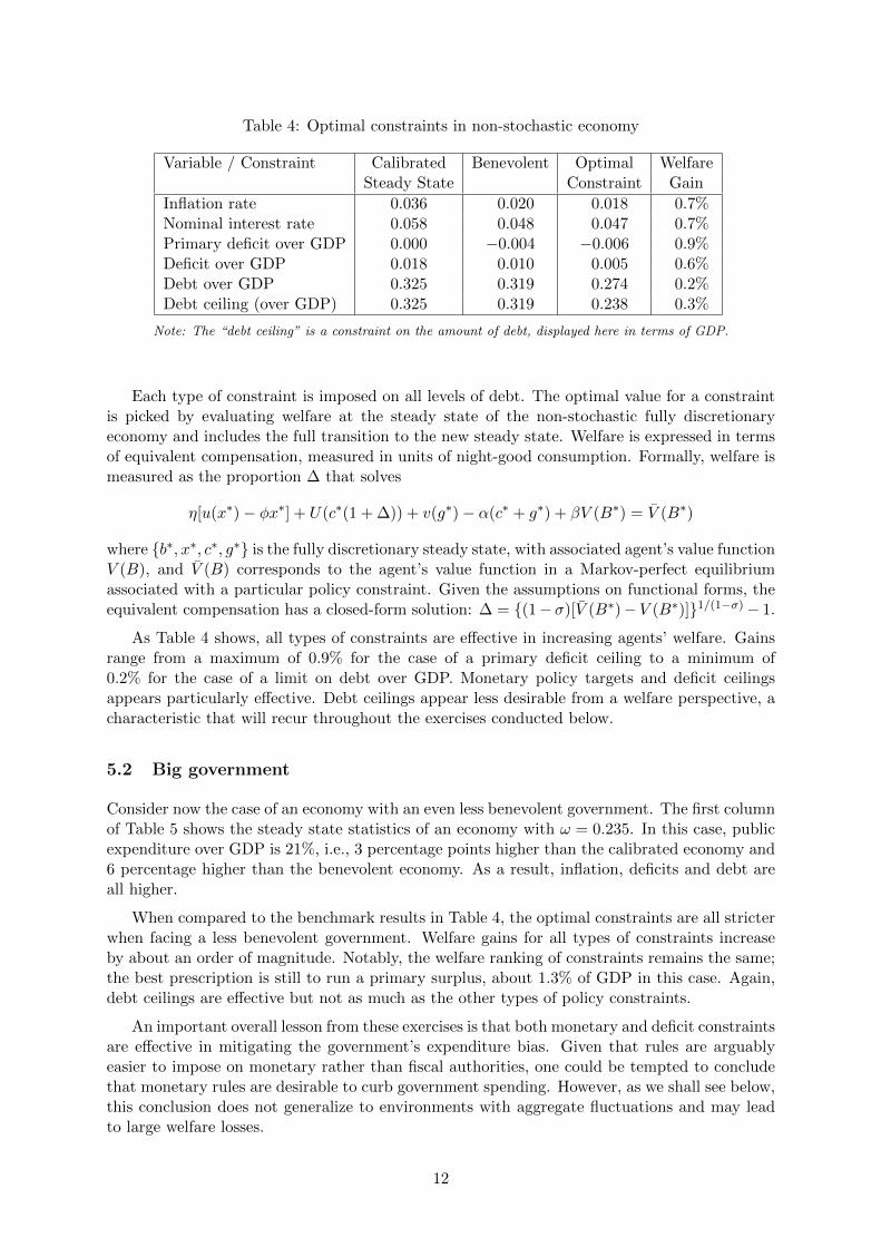
Table 4: Optimal constraints in non-stochastic economy

Variable / Constraint Calibrated Benevolent Optimal WelfareSteady State Constraint Gain

Inflation rate 0.036 0.020 0.018 0.7%Nominal interest rate 0.058 0.048 0.047 0.7%Primary deficit over GDP 0.000 −0.004 −0.006 0.9%Deficit over GDP 0.018 0.010 0.005 0.6%Debt over GDP 0.325 0.319 0.274 0.2%Debt ceiling (over GDP) 0.325 0.319 0.238 0.3%

Note: The “debt ceiling” is a constraint on the amount of debt, displayed here in terms of GDP.

Each type of constraint is imposed on all levels of debt. The optimal value for a constraintis picked by evaluating welfare at the steady state of the non-stochastic fully discretionaryeconomy and includes the full transition to the new steady state. Welfare is expressed in termsof equivalent compensation, measured in units of night-good consumption. Formally, welfare ismeasured as the proportion ∆ that solves

η[u(x∗)− φx∗] + U(c∗(1 + ∆)) + v(g∗)− α(c∗ + g∗) + βV (B∗) = V (B∗)

where {b∗, x∗, c∗, g∗} is the fully discretionary steady state, with associated agent’s value functionV (B), and V (B) corresponds to the agent’s value function in a Markov-perfect equilibriumassociated with a particular policy constraint. Given the assumptions on functional forms, theequivalent compensation has a closed-form solution: ∆ = {(1− σ)[V (B∗)− V (B∗)]}1/(1−σ)− 1.

As Table 4 shows, all types of constraints are effective in increasing agents’ welfare. Gainsrange from a maximum of 0.9% for the case of a primary deficit ceiling to a minimum of0.2% for the case of a limit on debt over GDP. Monetary policy targets and deficit ceilingsappears particularly effective. Debt ceilings appear less desirable from a welfare perspective, acharacteristic that will recur throughout the exercises conducted below.

5.2 Big government

Consider now the case of an economy with an even less benevolent government. The first columnof Table 5 shows the steady state statistics of an economy with ω = 0.235. In this case, publicexpenditure over GDP is 21%, i.e., 3 percentage points higher than the calibrated economy and6 percentage higher than the benevolent economy. As a result, inflation, deficits and debt areall higher.

When compared to the benchmark results in Table 4, the optimal constraints are all stricterwhen facing a less benevolent government. Welfare gains for all types of constraints increaseby about an order of magnitude. Notably, the welfare ranking of constraints remains the same;the best prescription is still to run a primary surplus, about 1.3% of GDP in this case. Again,debt ceilings are effective but not as much as the other types of policy constraints.

An important overall lesson from these exercises is that both monetary and deficit constraintsare effective in mitigating the government’s expenditure bias. Given that rules are arguablyeasier to impose on monetary rather than fiscal authorities, one could be tempted to concludethat monetary rules are desirable to curb government spending. However, as we shall see below,this conclusion does not generalize to environments with aggregate fluctuations and may leadto large welfare losses.

12

Table 5: Optimal constraints in non-stochastic economy with a big government

Variable / Constraint Big Benevolent Optimal WelfareGovernment Constraint Gain

Inflation rate 0.052 0.020 0.010 4.1%Nominal interest rate 0.068 0.048 0.042 4.1%Primary deficit over GDP 0.004 −0.004 −0.013 5.9%Deficit over GDP 0.025 0.010 −0.007 3.7%Debt over GDP 0.330 0.319 0.260 0.6%Debt ceiling (over GDP) 0.330 0.319 0.215 1.2%

Note: The “debt ceiling” is a constraint on the amount of debt, displayed here in terms of GDP.

6 Constrained Discretionary Policy

As a benchmark case, I consider an economy subjected to fluctuations in aggregate demand,i.e., with shocks to γ. In following sections, I verify that the main results obtained for demandshocks also apply to other types of shocks. In the analysis that follows, welfare associated witha particular stochastic environment is measured as the equivalent consumption compensationin state s2 (normal times), relative to the non-stochastic steady state, as defined in the previoussection. Welfare gains over full discretion are defined as the difference between welfare in aparticular (stochastic) constrained case and the fully discretionary (stochastic) equilibrium.

6.1 Optimal policy constraints

Table 6 summarizes the welfare effects of imposing constraints on policy in an economy facingdemand shocks. The four right-most columns show the welfare effects of imposing, respectively,policy constraints: (i) always; (ii) in normal and good times (suspended in bad times); (iii) innormal times only; and (iv) in bad and normal times (suspended in good times). The best caseis shown in bold. For each type of policy constraint, the column labeled “optimal value” showsthe value that corresponds to the best case (the best values for the remaining cases are omittedto simplify exposition).

Table 6: Welfare gains over full discretion

Constraint Optimal Always Suspended Only in Suspended

Value in bad times normal times in good times

Inflation rate 0.040 0.0% 0.0% 0.0% 0.0%Nominal interest rate 0.055 0.1% 0.1% 0.2% 0.1%P. Deficit over GDP −0.006 0.9% 0.8% 0.7% 0.8%Deficit over GDP 0.005 0.5% 0.5% 0.5% 0.5%Debt over GPD 0.272 0.1% 0.1% 0.1% 0.1%Debt ceiling (over GDP) 0.240 0.3% 0.2% 0.2% 0.2%

Note: The “debt ceiling” is a constraint on the amount of debt, displayed here in terms of GDP. For each type

of policy constraint,“optimal value” corresponds to the best scenario (bolded).

There are several important observations. First, placing an upper limit on the primarydeficit over GDP improves welfare the most. The optimal value is to have a small primarysurplus of about half a percent of output. Notably, this is the same result we obtained in the

13

non-stochastic case. Second, for all types of constraints, most of the welfare gains come fromimposing constraints in normal times. Third, suspending constraints during abnormal (bothbad and good) implies only small differences in welfare, for all types.

Figure 1 expands on the results summarized in Table 6. For each case, the figure plots thewelfare gains associated with imposing a particular policy constraint at specific times. Oneproperty that pops up is that, for each type of constraint, the optimal value is similar whetherwe allow the constraint to be sometimes suspended or not. As mentioned above, the welfarechanges of temporarily suspending constraint is minor relative to the overall welfare gains ofimposing them in the first place. Both these results are significant for implementation, as theremay be other reasons (say, political) for wanting to suspend constraint on government actionsat certain times. Note, however, that these conclusions rely on the fact that constraints are tobe reimposed when normal times come back.

Figure 1: Welfare gains over full discretion

‐0.25%

‐0.20%

‐0.15%

‐0.10%

‐0.05%

0.00%

0.05%

0.030 0.035 0.040 0.045 0.050

Inflation Rate

Always Suspend in bad Normal only Suspend in good

‐0.20%

0.00%

0.20%

0.40%

0.60%

0.80%

1.00%

‐0.010 ‐0.005 0.000

P. Deficit over GDP

Always Suspend in bad Nomal only Suspend in good

‐0.40%

‐0.30%

‐0.20%

‐0.10%

0.00%

0.10%

0.20%

0.050 0.055 0.060

Nominal Interest Rate


‐0.10%

0.00%

0.10%

0.20%

0.30%

0.40%

0.50%

0.60%

0.000 0.005 0.010 0.015 0.020

Deficit over GDP


‐0.20%‐0.15%‐0.10%‐0.05%0.00%0.05%0.10%0.15%0.20%

0.25 0.30 0.35 0.40

Debt over GDP


‐0.10%

0.00%

0.10%

0.20%

0.30%

0.20 0.25 0.30 0.35 0.40

Debt Ceiling


6.2 The cost of mistakes

Is it costly to set the wrong value for a constraint? As Figure 1 illustrates, it depends on thetype of constraint. Imposing constraints on the deficit is generally benign (at least, as long aswe do not impose an overly strict constraint). For example, small primary surpluses are alwaysbeneficial, so getting the exact value for the constraint right is not critical, which is an addedbenefit as it reduces the costs of incorrect implementation. In contrast, monetary policy targetscan quickly turn a gain into a (large) loss. Coupled with the fact that the welfare gains of theoptimal value are fairly small to begin with, this implies that monetary targets are not desirableconstraints. This is an important result that would have been missed if we had not looked at astochastic economy.

Debt constraints are good as long as they are not too tight, as they interact with the abilityof the government to smooth distortions. A limit on debt over GDP, as the one imposed onEurozone countries, has the peculiar property of two local maxima. Note however, that thestricter limit yields higher welfare. The welfare gains of a debt ceiling, as the one implementednominally in the US, are single peaked, but note that they rapidly convert into losses when itis set too high. The reason for this result is that debt ceilings hinder distortion-smoothing evenif suspended during abnormal times.

14

6.3 Policy dynamics

Figure 2 compares the policy response to a negative demand shock under full discretion vs theoptimal primary deficit ceiling, as indicated by the results in Table 6. The charts start off eacheconomy at the non-stochastic steady state level of debt, 10 periods before the negative shockhits. This shock lowers real GDP by about 10% for 10 years (which is the calibrated durationof the bad state). The economy then returns to normal.

Figure 2: Full discretion vs optimal primary deficit ceiling

0%

10%

20%

30%

40%

50%

‐10 ‐5 0 5 10 15 20 25 30

Debt / GDP

‐2%

‐1%

0%

1%

2%

‐10 ‐5 0 5 10 15 20 25 30

Primary Deficit / GDP

0%

2%

4%

6%

8%

‐10 ‐5 0 5 10 15 20 25 30


0%

2%

4%

6%

8%

‐10 ‐5 0 5 10 15 20 25 30

Expected Inflation

Note: full discretion (red solid line) and primary deficit ceiling (light blue line).

The constrained policy displays a significantly more muted response to the adverse shock.The better welfare performance of the optimal primary deficit constraint comes from the lowerinflation distortion it allows. In effect, by implementing a primary surplus, inflation can belower, both in normal and adverse times. In the appendix, Figure 5 shows the implied dynamicsin allocations. Lower inflation under the deficit constraint is associated with higher day-goodconsumption. Notably, under the primary deficit constraint day-good consumption does notreact significantly once the adverse shock hits. The optimal policy constraint also implies lowerpublic expenditure. They drop significantly more during bad times, which explains why notsuspending the constraint leads to larger welfare gains.

Figure 3 considers the case when we allow for the primary deficit ceiling to be suspendedin abnormal times. As shown in Table 6, most of the welfare gains from a primary deficitceiling came from imposing it during normal times. The constrained policy response looks nowqualitatively more similar to the fully discretionary policy. There are two important differences.

15

First, during normal times, the requirement of a primary surplus induces a lower inflation thanunder discretion, which mitigated the social losses due to political frictions. Second, when theeconomy returns to normal, both debt and inflation transition gradually back to their (long-run)normal levels. I.e., even though the government is constrained to run a surplus, it is still ableto adequately smooth distortions over time, which is always desirable. This is why an inflationtarget imposed during normal times only (of say 2% annual) does not work as effectively;although inflation is typically lower, once the economy returns back to normal, inflation needsto adjust immediately, which is costly since it does not allow for sufficient distortion-smoothing.

Figure 3: Full discretion vs optimal primary deficit ceiling in only normal times

0%

10%

20%

30%

40%

50%

‐10 ‐5 0 5 10 15 20 25 30

Debt / GDP

‐2%

‐1%

0%

1%

2%

‐10 ‐5 0 5 10 15 20 25 30

Primary Deficit / GDP

0%

2%

4%

6%

8%

‐10 ‐5 0 5 10 15 20 25 30


0%

2%

4%

6%

8%

‐10 ‐5 0 5 10 15 20 25 30

Expected Inflation

Note: full discretion (red solid line) and primary deficit ceiling in normal times only (light bluedashed line).

6.4 Welfare and the timing of reform

Another potential concern is the fact that constraints could be imposed at inappropriate times.For example, the calculations for optimal constraints rely on them being implemented aroundthe non-stochastic steady state (which is trivially close to the stochastic steady state in normaltimes with full discretion). What happens when constraints are placed far from this state?In particular, how does the welfare derived from imposing the optimal values for each policyconstraint depend on the level of debt at the moment of introduction? Figure 4 provides ananswer to this question.

The optimal inflation target can lead to some important welfare losses when implemented far

16

from the steady state. These losses increase dramatically when imposing the optimal interestrate target. In fact, there is only a small range of debt levels over which monetary policyconstraints are welfare improving. The optimal primary deficit target typically leads to fairlyconsistent welfare gains, even when initial debt is fairly high. The exception is when initialdebt is low, as the requirement of a primary deficit surplus severely limits the amount of debtaccumulation and thus, mitigates distortion-smoothing. On the other hand, the optimal deficitceiling offers consistent welfare gains for all levels of debt. The difference stems from the factthat at low levels of debt, the constrained government can now run a primary deficit, since theinterest paid on debt is low. Hence, a deficit ceiling, as opposed to a primary deficit ceiling,might be a better idea for governments with low initial debt. Both debt constraints can lead tosubstantial welfare losses when initial debt is high. The reason for this is simple: the debt ceilingforces a sudden adjustment of debt, which goes against the desirability to smooth distortions.

Figure 4: Welfare gains of optimal constraints as a function of initial debt level

‐2.0%

‐1.5%

‐1.0%

‐0.5%

0.0%

0.5%

1.0%

0% 10% 20% 30% 40% 50% 60% 70%

Welfare gains over F

ull D

iscretion

Debt / GDP

Inflation Interest rate P. Deficit/GDP Deficit/GPD Debt/GDP Debt ceiling

Monetary targets (inflation and interest rates) have a minor upside and are instead poten-tially very costly when implemented far away from the non-stochastic steady state. Coupledwith the findings in Figure 1, this suggests that monetary targets are generally not a good ideain economies with potentially large aggregate demand shocks. In contrast, as shown in Ta-bles 4 and 5, they improve welfare significantly in non-stochastic economies (and by extension,probably also in economies subjected to very mild aggregate fluctuations).

6.5 Frequent abnormal times

Next we consider increasing the frequency of abnormal times or, equivalently, reducing theduration of normal times. Let $∗ = $ = 0.9; that is, all states have now a duration of 10 years.Table 7 present the results. As we can see, the results obtained for the benchmark case stillapply. Even the optimal values for constraint are very close. The only significant difference isa slight decrease in welfare gains.

17

Table 7: Welfare gains over full discretion when abnormal times are frequent



Inflation rate 0.040 −0.0% 0.0% 0.0% 0.0%Nominal interest rate 0.055 −0.2% 0.0% 0.1% 0.0%P. Deficit over GDP −0.007 0.8% 0.5% 0.3% 0.5%Deficit over GDP 0.005 0.5% 0.4% 0.3% 0.4%Debt over GDP 0.272 0.1% 0.1% 0.1% 0.1%Debt ceiling (over GPD) 0.240 0.2% 0.2% 0.2% 0.2%



6.6 Distortion-smoothing vs time-consistency

What role is the time-consistency problem playing in the results? One simple way to address thisquestions is to slightly modify the government’s GEE (8) by weighting the distortion-smoothingand time-inconsistency terms. Specifically, let ξ ∈ (0, 1) weight the relative importance of thesemotives, so that (8) gets replaced by:

ξE

[φx′(1− θ′)(λ− Λ′)

(1 + θ′B′)2

∣∣∣s] + (1− ξ)λ(s)E

[X ′B

{η(u′x + u′xxx

′ − φ) +φ(1 +B′)

1 + θ′B′

} ∣∣∣s] = 0

The limited commitment government analyzed thus far corresponds to the case ξ = 1/2. As ξgoes to zero, we approach the case of a government with commitment, who would ignore thetime-consistency problem of its policy prescription and care solely about distortion-smoothing.As ξ increases, the time-consistency motive starts to weight more and more in the government’splan.

Table 8: Welfare gains over full discretion as a function of ξ

0.1 0.2 0.3 0.4 0.5 0.6 0.7 0.8

−0.018% −0.007% −0.004% −0.002% 0.000% 0.001% −0.001% −0.014%

Table 8 shows the effects of varying ξ. In general, welfare is lower when the governmenthas either a distortion-smoothing or a time-consistency bias. The optimal value for ξ is around0.6, which implies that a small time-consistency bias may be desirable. Note however, thatwelfare gains are tiny. This exercise highlights the inability of commitment to policy actions(as represented by a low ξ) to counter the distortions created by political frictions, a result thatgeneralizes the lesson from Proposition 1. It is constraints on government action (itself a formof commitment) rather than pre-commitment to a course of action that results in an effectivemitigation of the expenditure bias.

6.7 Other shocks

We now verify that the main results derived for aggregate demand shocks also apply to othertypes of shocks. Table 9 summarizes the welfare effects of imposing constraints on policy ineconomies facing productivity, liquidity and government expenditure shocks.

18

Table 9: Welfare gains over full discretion

Productivity shocks



Inflation rate 0.040 −0.2% −0.1% 0.0% −0.1%Nominal interest rate 0.055 0.0% 0.1% 0.2% 0.1%P. Deficit over GDP −0.007 0.9% 0.8% 0.7% 0.7%Deficit over GDP 0.005 0.6% 0.6% 0.5% 0.5%Debt over GPD 0.272 0.2% 0.2% 0.1% 0.1%Debt ceiling (over GDP) 0.240 0.3% 0.3% 0.2% 0.2%

Liquidity shocks



Inflation rate 0.040 0.0% 0.0% 0.0% 0.0%Nominal interest rate 0.055 −0.3% −0.1% 0.1% −0.2%P. Deficit over GDP −0.006 0.8% 0.8% 0.7% 0.8%Deficit over GDP 0.005 0.6% 0.5% 0.5% 0.5%Debt over GPD 0.325 0.1% 0.1% 0.1% 0.1%Debt ceiling (over GDP) 0.284 0.3% 0.3% 0.2% 0.3%

Government expenditure shocks



Inflation rate 0.040 0.0% 0.0% 0.0% 0.0%Nominal interest rate 0.056 0.2% 0.1% 0.1% 0.2%P. Deficit over GDP −0.007 1.1% 0.7% 0.6% 1.1%Deficit over GDP 0.004 0.7% 0.5% 0.4% 0.7%Debt over GPD 0.325 0.2% 0.2% 0.2% 0.2%Debt ceiling (over GDP) 0.285 0.4% 0.3% 0.3% 0.3%



Although each case presents its own idiosyncracies, the similarities across economies arenotable. For each type of shock the best prescription remains a small primary surplus, between0.6% and 0.7% of GDP. It is always best not to suspend this constraint. Again, even if theconstraint is imposed only during normal times, due to the distortion-smoothing motive, it isdisciplining government behavior during abnormal times. Except for the case with expenditureshocks, the welfare loss of suspending a primary deficit constraint during abnormal times (good,bad or both) is very small. The same conclusions can be drawn about imposing the nextbest constraint, a ceiling on total deficit over GDP of around 0.4% to 0.5%. For economieswith expenditure shocks, since the spending increase stems from the government becoming lessbenevolent, the gains from not suspending deficit constraints during bad times are significant.

Monetary policy constraints remain largely undesirable. There are many cases in whichthese constraints lead to welfare losses relative to full discretion. Ironically, their performanceis especially poor in the presence of liquidity shocks. When they do improve over discretion, it

19

is in the form of an interest rate target and the gains are small. Debt constraints fare better,especially a debt ceiling that is imposed at all times. Still the gains from debt constraints aredominated by those deficit constraints, even when they are not implemented optimally.

7 General Lessons and Conclusions

The exercises presented in this paper offer some important and novel lessons for the institutionaldesign of government policy.

First, a small primary surplus is always the best policy and it is never optimal to suspend thisconstraint. For an economy calibrated to the U.S. and subject to a variety of shocks, the optimalprimary surplus is a bit over half percent of output. A total deficit of about half a percent ofoutput, imposed at all times, is the next best prescription. In both cases, most welfare gainscome from imposing constraints in normal times, which also helps discipline government policyduring abnormal times. The cost of implementing deficit constraints sub-optimally, e.g., pickingthe wrong ceiling or suspending constraints during abnormal times, carry small welfare costs. Anotable exception is suspending deficit constraints when government expenditure temporarilyincreases (assuming agents do not value such an increase). Welfare gains from deficit constraintsare still significant even when they are implemented far from steady state; the only exceptionbeing imposing a primary deficit ceiling with very low debt.

Second, monetary policy rules, i.e., inflation and interest rate targets, are not generallydesirable constraints. In economies with no aggregate fluctuations, these constraints performactually quite well, yielding welfare gains similar to those of deficit constraints. However, in thepresence of aggregate shocks of various types, monetary policy targets yield small welfare gainsand losses relative to full discretion. More problematic is the fact that slight mis-targeting orincorrect timing can lead to large welfare losses. The reason for these negative results is thatmonetary policy targets hinder the ability of governments to smooth distortions across states.In effect, inflation allows for less distortionary repayments of temporary debt increases.

Third, debt limits are generally effective, but are always dominated by deficit constraints,even when these latter constraints are not implemented at their best (e.g., because societyallows them to be suspended in bad times). This suggest that the typical focus of governmentreformers on debt ceilings may be misplaced. It is always more desirable, and arguably easierin practice, to aim at constraining the deficit.

Fourth, and not least, the socially effective way to combat inefficiently high public expendi-ture, is not more pre-commitment to government actions, but rather commitment to rules thatconstraint government action. The difference is that the latter makes the government internalizethe cost of socially suboptimal policy.

20

References

Aiyagari, S. R., Marcet, A., Sargent, T. J. and Seppala, J. (2002), ‘Optimal taxation withoutstate-contingent debt’, The Journal of Political Economy 110(6), 1220–1254.

Albanesi, S., Chari, V. V. and Christiano, L. J. (2003), ‘Expectation traps and monetary policy’,The Review of Economic Studies 70(4), 715–741.

Azzimonti, M., Battaglini, M. and Coate, S. (2010), Analyzing the case for a balanced budgetamendment to the U.S. constitution. Mimeo.

Barro, R. J. (1979), ‘On the determination of the public debt’, The Journal of Political Economy87(5), 940–971.

Barro, R. J. and Gordon, D. B. (1983), ‘A positive theory of monetary policy in a natural-ratemodel’, The Journal of Political Economy 91, 589–610.

Barseghyan, L. and Battaglini, M. (2012), Growth and fiscal policy: a positive theory. Mimeo.

Bassetto, M. and Sargent, T. J. (2006), ‘Politics and efficiency of separating capital and ordinarygovernment budgets’, The Quarterly Journal of Economics 121(4), 1167–1210.

Benhabib, J. and Rustichini, A. (1997), ‘Optimal taxes without commitment’, Journal of Eco-nomic Theory 77(2), 231–259.

Bohn, H. and Inman, R. P. (1996), ‘Balanced-budget rules and public deficits: evidence fromthe U.S. states’, Carnegie-Rochester Conference Series on Public Poliy 45, 13–76.

Brennan, G. and Buchanan, J. M. (1977), ‘Towards a tax constitution for leviathan’, Journalof Public Economics 8, 255–273.

Chari, V. and Kehoe, P. J. (2007), ‘On the need for fiscal constraints in a monetary union’,Journal of Monetary Economics 54, 23992408.

Halac, M. and Yared, P. (2012), Fiscal rules and discretion under persistent shocks. Mimeo.

Harchondo, J. C., Martinez, L. and Roch, F. (2012), Fiscal rules and the sovereign defaultpremium. Working Paper 12-01, The Federal Reserve Bank of Richmond.

Kiyotaki, N. and Moore, J. (2002), ‘Evil is the root of all money’, American Economic Review92(2), 62–66.

Kocherlakota, N. (1998), ‘Money is memory’, Journal of Economic Theory 81, 232–251.

Kydland, F. E. and Prescott, E. C. (1977), ‘Rules rather than discretion: The inconsistency ofoptimal plans’, The Journal of Political Economy 85(3), 473–491.

Lagos, R. and Wright, R. (2005), ‘A unified framework for monetary theory and policy analysis’,The Journal of Political Economy 113(3), 463–484.

Lucas, R. E. and Stokey, N. L. (1983), ‘Optimal fiscal and monetary policy in an economywithout capital’, Journal of Monetary Economics 12(1), 55–93.

Martin, F. M. (2009), ‘A positive theory of government debt’, Review of Economic Dynamics12(4), 608–631.

Martin, F. M. (2010), ‘Markov-perfect capital and labor taxes’, Journal of Economic Dynamicsand Control 34(3), 503–521.

21

Martin, F. M. (2011), ‘On the joint determination of fiscal and monetary policy’, Journal ofMonetary Economics 58(2), 132–145.

Martin, F. M. (2012), ‘Government policy response to war-expenditure shocks’, The B.E. Jour-nal of Macroeconomics 12(1), (Contributions), Article 25.

Martin, F. M. (2013), ‘Government policy in monetary economies’, International EconomicReview 54(1), 185–217.

Martin, F. M. (2015), ‘Debt, inflation and central bank independence’, European EconomicReview 79, 129–150.

Martin, F. M. and Waller, C. J. (2012), ‘Sovereign debt: a modern Greek tragedy’, Review,Federal Reserve Bank of St. Louis (Issue Sep), 321–340.

Mishkin, F. S. (1999), ‘International experiences with different monetary policy regimes’, Jour-nal of Monetary Economics 43(3), 579–605.

Ohanian, L. E. (1997), ‘The macroeconomic effects of war finance in the United States: WorldWar II and the Korean War’, American Economic Review 87(1), 23–40.

Shi, S. (2006), ‘Viewpoint: A microfoundation of monetary economics’, Canadian Journal ofEconomics 39(3), 643–688.

Strotz, R. H. (1956), ‘Myopia and inconsistency in dynamic utility maximization’, The Reviewof Economic Studies 23(3), 165–180.

Svensson, L. E. O. (1999), ‘Infation targeting as a monetary policy rule’, Journal of MonetaryEconomics 43(3), 607–654.

Wallace, N. (2001), ‘Whither monetary economics?’, International Economic Review 42(4), 847–869.

Williamson, S. and Wright, R. (2010), New monetarist economics: Models, in B. M. Fried-man and M. Woodford, eds, ‘Handbook of Monetary Economics’, Vol. 3, North Holland,Amsterdam.

22

A Demand shock

Figure 5: Full discretion vs optimal primary deficit ceiling

‐1.5%

‐1.0%

‐0.5%

0.0%

0.5%

1.0%

1.5%

2.0%

‐10 ‐5 0 5 10 15 20 25 30

Day‐Good Consumption

‐15%

‐10%

‐5%

0%

5%

‐10 ‐5 0 5 10 15 20 25 30

Night‐Good Consumption

‐15%

‐10%

‐5%

0%

5%

‐10 ‐5 0 5 10 15 20 25 30

Night‐Labor

‐1.5%

‐1.0%

‐0.5%

0.0%

0.5%

‐10 ‐5 0 5 10 15 20 25 30

Public Good Consumption

Note: full discretion (red solid line) and primary deficit ceiling (light blue line). Each allocationis shown as deviations from non-stochastic steady state.

23

Documents

The Value of Constraints on Discretionary Government Policy · PDF filediscussion and critical comment. ... El Salvador and Panama all use the U.S. dollar. In practice, however,