THE VALUE OF WIND PROFILER DATA IN U.S. WEATHER …

1871DECEMBER 2004AMERICAN METEOROLOGICAL SOCIETY |

T he National Oceanic and Atmospheric Admin-istration (NOAA) Forecast Systems Laboratory(FSL) has operated a network of 404-MHz tro-

pospheric wind profilers since 1992 (online atwww.profiler.noaa.gov/jsp/aboutNpnProfilers.jsp; vande Kamp 1993; Weber et al. 1990). Most of these plat-forms operate over the central United States, with theexception of a few profilers in Alaska and elsewhere(Fig. 1). The role of wind profiler data in forecasterdecision making is typified in the following two ac-counts regarding significant weather events:

The NOAA Storm Prediction Center (SPC) inNorman, Oklahoma, located in the middle of the

NOAA Profiler Network (NPN), has a high interestin monitoring evolving low-level and deep verticalwind shear that is conducive to severe thunder-storms. SPC forecasters frequently use the profilerdata for issuing both convective outlooks as well aswatches, with the data often critical for determin-ing the level of severity expected. A prime exampleoccurred with the 3 May 1999 Oklahoma–Kansas

THE VALUE OF WIND PROFILERDATA IN U.S. WEATHER

FORECASTINGBY STANLEY G. BENJAMIN, BARRY E. SCHWARTZ, EDWARD J. SZOKE,* AND STEVEN E. KOCH

Severe-weather cases and a winter test period show that the NOAA wind profiler network

in the central United States can improve short-range (3-12 h) forecasts.

AFFILIATIONS: BENJAMIN, SCHWARTZ, SZOKE, AND KOCH—NOAA/Forecast Systems Laboratory, Boulder, Colorado*Additional affiliation: Cooperative Institute for Research in theAtmospheres, Colorado State University, Fort Collins, ColoradoA supplement to this article is available online (DOI:10.1175/BAMS-84-11-Benjamin)CORRESPONDING AUTHOR: Stan Benjamin, NOAA/FSL, 325Broadway, R/E/FS1, Boulder, CO 80305E-mail: [email protected]:10.1175/BAMS-85-12-1871

In final form 24 June 2004”2004 American Meteorological Society

FIG. 1. NPN site locations as of Aug 2002. The LDBT2site in southeastern Texas was not operational for thecases in May 1999 and February 2001 discussed in thispaper. RASS (Martner et al. 1993) observations, includ-ing lower-tropospheric profiles of virtual temperature,were not used in this study.

1872 DECEMBER 2004|

tornado outbreak (Edwards et al. 2002). The fore-casters on 3 May observed considerably strongerwinds at the Tucumcari, New Mexico, profiler sitethan were forecasted by the models. Extrapolationof these winds to the afternoon threat area gave theforecasters confidence that tornadic storms withorganized supercells would be the main mode ofsevere weather risk. Based on the likelihood of stron-ger vertical wind shear, the risk would be greaterthan that previously suggested by numerical mod-els. Armed with the profiler observations, SPC fore-casters first increased the threat in the current-dayconvective outlook from slight to moderate risk, andthen to high risk by early afternoon. Such changesare regarded seriously by response groups such asemergency managers, and the elevated risk levelsfrom SPC resulted in a more intense level of civic andgovernment response (Morris et al. 2002) to this po-tential tornado threat. In fact, NOAA’s Service As-sessment Report for the 3 May 1999 tornadoes(NWS 1999) noted the critical role that the profilerdata had in improving the forecasts (convective out-looks and watches) from the SPC, and recom-mended that the existing profiler network be sup-ported as a reliable operational data source(S. Weiss, 2002, personal communication).

The National Weather Service Forecast Office inSioux Falls, South Dakota, described a wintertimeapplication of profiler data: “Tonight the profilernetwork was useful for determining the end time ofsnowfall which coincided with the mid-level troughpassage. We had a main trough passage produce upto 6 inches (of snow) and a secondary trough pro-duce areas of IFR (Instrument Flight Rules) condi-tions but no accumulating snow. The profilers areused almost daily by the forecasters in this office”(P. Browning, 2002, personal communication).

The two previous paragraphs describe examples ofwind profiler data use by operational forecasters. Inthis article, we discuss the use of profiler data in bothnumerical weather prediction (NWP) and subjectiveweather forecasting in three aspects. First, a series ofexperiments was performed using the Rapid UpdateCycle (RUC) model and hourly assimilation system(Benjamin et al. 2004a,b) for a 13-day period in Feb-ruary 2001 comprised of a control experiment withall data and a series of denial experiments in whichdifferent sets of observations were withheld. Datadenial experiments were conducted denying profilerand aircraft data. For the control and denial experi-ments withholding profiler, aircraft, and all data, av-erage verification statistics for RUC wind forecasts

against radiosonde observations were compiled forthe test period. The day-to-day differences in these er-rors and in profiler impact were also calculated. In ad-dition to the average root-mean-square (rms) windvector errors, statistics were compiled for the 5% larg-est errors at individual radiosonde locations to focuson the impact of data denial for peak error events.Significance tests were performed for the differencebetween experiments with and without profiler data.

Second, three case studies illustrating the positiveimpact of profiler data on RUC forecasts are discussedbriefly in section 3 and in more detail in Benjaminet al. (2004c). For each case study, reruns of the RUCwith and without profiler data are contrasted. The firstcase is derived from RUC forecasts of the 3 May 1999Oklahoma tornado outbreak. The second case studyis taken from the 13-day test period for a significantsnow and ice storm that affected parts of Oklahoma,Kansas, Nebraska, and Missouri on 9 February 2001.The third case is for a tornadic event in central Okla-homa on 8 May 2003 that closely followed the trackof the most destructive tornado on 3 May 1999.

DATA-DENIAL EXPERIMENTS USING THERUC MODEL. Observation system experiments(OSEs) have been found to be very useful in determin-ing the impact of particular observation types on op-erational NWP systems (e.g., Graham et al. 2000;Bouttier 2001; Zapotocny et al. 2002). Four multidayRUC experiments (or OSEs) with an assimilation ofdifferent observational mixes were performed for the4–17 February 2001 period. This 13-day period wascharacterized by strong weather changes across theUnited States and has been used for retrospective test-ing at the National Centers for Environmental Pre-diction (NCEP) for modifications to the Eta and RUCmodel systems. During this period, at least three ac-tive weather disturbances traversed the profiler net-work, including the severe ice and snow that affectedparts of the U.S. central plains on 8–9 February 2001.This case is discussed in more detail in section titled“Case studies.”

Experimental design. The version of the RUC used inthese experiments is the 20-km version run opera-tionally at NCEP as of June 2003, including 50 hy-brid isentropic-sigma vertical levels and advancedversions of modeled physical parameterizations. Anhourly intermittent assimilation cycle allows full useof hourly profiler (and other high frequency) obser-vational datasets. The analysis method is the three-dimensional variational data assimilation (3DVAR)technique (Devenyi and Benjamin 2003; Benjamin


et al. 2003) implemented in the operational RUC inMay 2003. Additional information about the 20-kmRUC is provided by Benjamin et al. (2002, 2004a,b).The experiment period began at 0000 UTC 4 Febru-ary 2001 with the background provided from a 1-hRUC forecast initialized at 2300 UTC 3 February.Lateral boundary conditions were specified from theNCEP Eta Model initialized every 6 h and availablewith a 3-h-output frequency. The high-frequency ob-servations used include those from wind profilers,commercial aircraft, Doppler radar velocity azimuthdisplay (VAD) wind profiles, and surface stations. NoRadio Acoustic Sounding System (RASS; e.g.,Martner et al. 1993) temperature profiles, also avail-able at many NPN sites (Fig. 1), were used in any ofthese experiments because they are not yet availablein the operational data stream at NCEP.

Verification was performed using conventional12-hourly radiosonde data over the three domains de-picted in Fig. 2. The entire RUC domain contains ~90radiosonde sites. The solid box outlining the profilersubdomain includes most of the Midwest profilersdepicted in Fig. 1 and contains 22 radiosonde sites.

The dashed box area in Fig. 2, referred to as the“downstream” subdomain, contains 26 radiosondesites. It was chosen to depict an area that might beaffected due to downstream propagation of informa-tion originating from the profiler data. For each RUCexperiment, residuals (forecast minus observed) werecomputed at all radiosonde locations located withineach respective verification domain. Next, the rmsvector difference between forecasts and observationswas computed for each 12-h verification time. Thisdifference is sometimes referred to below as “forecasterror,” but in fact also contains a contribution fromthe observation error (including representativeness“error” from the inability of a grid to resolve subgridvariations sometimes evident in observations). Thesescores were then averaged linearly over the 13-day testperiod. In many of the figures that follow, the statis-tic displayed is a difference between these averagescores: the control (RUC run with all data, henceforthreferred to as CNTL) minus the experiment (noprofiler, no aircraft, or no observations at all; hence-forth referred to as EXP). In addition, the Student’s ttest was performed on the differences between the

FIG. 2. The full 20-km RUC domain with terrain elevation (m), with outlines of profiler (solid line) anddownstream (dotted line) verification subdomains.

1874 DECEMBER 2004|

CNTL and EXP standard deviations of the residualsto determine statistical significance of the results.Finally, the mean differences were normalized bythree different methods to clarify their contributionto forecast error, as described in the “Normalized re-sults for profiler and aircraft data denial experiments”section. Quality-control flags from RUC analyses in theCNTL cycle were applied to verifying radiosonde data.

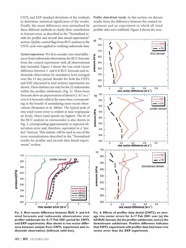
Control experiment. We first consider rms wind differ-ences from radiosonde observations for RUC forecastsfrom the control experiment with all observationaldata included. Figure 3 shows the rms wind vectordifference between 3- and 6-h RUC forecasts and ra-diosonde observations by mandatory level averagedover the 13-day period. Results for both the CNTLand EXP (discussed in next section) experiments areshown. These statistics are only for the 22 radiosondeswithin the profiler subdomain (Fig. 2). Three-hourforecasts show an improvement of about 0.2–0.7 m s-1

over 6-h forecasts valid at the same time, correspond-ing to the benefit of assimilating more recent obser-vations (Benjamin et al. 2004a). The typical peak ofrms wind vector error is evident at near-tropopausejet levels, where wind speeds are highest. The fit ofthe RUC analysis to rawinsondes is also shown inFig. 3, corresponding approximately to expected ob-servation error and, therefore, equivalent to a “per-fect” forecast. This statistic will be used in one of thescore normalizations described in the “Normalizedresults for profiler and aircraft data denial experi-ments” section.

Profiler data-denial results. In this section, we discussresults from the difference between the control ex-periment and an experiment in which all windprofiler data were withheld. Figure 4 shows the aver-

FIG. 3. Rms vector difference between RUC 3- and 6-hwind forecasts and radiosonde observations overprofiler subdomain for 4–17 Feb 2001 period for CNTLand EXP experiments. Also shown is rms vector differ-ence between analysis from CNTL experiment and ra-diosonde observations (leftmost solid line).

FIG. 4. Effects of profiler data denial (CNTL) on aver-age rms vector errors for 4–17 Feb 2001 over (a) thefull RUC domain, (b) the profiler subdomain, and (c) thedownstream subdomain. Positive difference indicatesthat CNTL experiment with profiler data had lower rmsvector error than the EXP experiment.


age 3-, 6-, and 12-h wind forecast impact (EXP – CNTL)results for the 4–17 February test period (rms vectorscore from each radiosonde verification time averagedover each period) for the three different verificationdomains. This score, reflecting the impact of windprofiler data, is positive for all levels and all domains.As expected, the greatest impact at 3 h is evident overthe profiler subdomain (Fig. 4b), from 0.3 to 0.6 m s-1

at all mandatory levels (850–150 hPa), with an aver-age value of 0.46 m s-1 (Table 1). By contrast, the 3-hvertically averaged impact is 0.28 m s-1 over the down-stream domain and 0.21 m s-1 over the full RUC do-main. In general, the impact decreases with increasedforecast projection. The 12-h-forecast impact is quitesmall over the three verification domains (< 0.1 m s-1).[Plots of wind forecast error from different RUC fore-casts for a particular case are shown in Benjamin et al.(2004b, Fig. 11), illustrating that differences in rmsvector error of 0.5 m s-1 are easily apparent in visualinspection.]

A stratification of profiler impact results by thetime of day over the profiler subdomain (Fig. 5) re-vealed that the profiler impact is stronger at 1200 thanat 0000 UTC at most vertical levels. This is likely aresult of a lower volume of aircraft data in the 0600–0900 UTC nighttime period than the 1800–2100 UTCdaytime period (3-h periods preceding the initial timefor 3-h forecasts valid at 1200 or 0000 UTC). It alsoshows that the profiler data can contribute stronglyto improving wind forecast at near-tropopause jetlevels and that the accuracy of 3-h jet-level wind fore-casts valid at 1200 UTC over the United States isstrengthened by wind profiler data.

The statistical significance of mean absolute (notrms) CNTL – EXP differences for 3–12-h forecasts bymandatory levels is examined with the Student’s t testin Table 2. The difference between 3-h forecasts withand without profiler data is statistically significant atthe 99% confidence level for the 700–400-hPa levels.The difference for 6-h forecasts was significant at the80% level or higher at three levels in the profiler and

3 h 6 h 12 h

Domain Mean diff Mean diff Mean diff

TABLE 1. Mean reduction in rms wind vectorerror (m s-----1) from EXP to CNTL experimentsover Feb 2001 test period, averaged over eightmandatory pressure levels.

Profiler 0.46 0.25 0.07

Downstream 0.28 0.19 0.06

Full RUC 0.21 0.13 0.03

FIG. 5. Diurnal variability of profiler impact (CNTL) onrms 3-h wind forecast vector error in profilersubdomain. Same as Fig. 4b, but with separate resultsfor 0000 and 1200 UTC.

FIG. 6. Time series of 500-hPa wind rms vector differ-ences between forecasts and radiosonde observationsover profiler subdomain for 5–17 Feb (Julian date 36–48) 2001 period. Values are shown for 3-h RUC fore-casts from control experiment (03h) and 3-h persis-tence forecasts (03p, using RUC analyses valid at 0900and 2100 UTC), also from the control experiment.

downstream domains and for five of eight mandatorylevels over the full RUC domain.

In considering multiday experiments to test fore-cast impact from some change, a problem with anylong-period average statistic is that it may mask thepotentially more significant impact associated withlarger errors in active weather events. In Fig. 6, a timeseries is shown of the 3-h RUC and persistence fore-cast 500-hPa wind vector errors from the control ex-periment at each 12-h verification time. The 3-h per-sistence forecast is determined simply as the RUCCNTL analysis from 3 h before the verification time.

1876 DECEMBER 2004|

There are three higher error events (over the profilersubdomain) evident in this figure for 5, 10, and16 February (Julian dates 36, 41, and 47, respectively),which are all associated with the passage of strongupper-level waves. The 3-h persistence errors peak

much more sharply than the3-h forecast error, indicatingthat the rapid changes in the500-hPa wind field are largely,but not completely, capturedby the model forecasts.

A time series of the profilerimpact at each 12-h verificationtime (0000 and 1200 UTC) atselected mandatory pressuresurfaces (Fig. 7) reveals signifi-cant day-to-day variations inthe profiler impact. Comparingtime series of 500-hPa persis-tence error (Fig. 6) and profilerimpact (Fig. 7) shows some cor-relation between larger profilerimpact (at 850 hPa on 5 and10 February, and at 500 hPa on16 February) and more change-able weather situations. Figure 7also shows that the time-by-time impact from profiler datais usually positive. Intermittentnegative impacts evident inFig. 7 are attributed to aliasing,which can occur from any insitu observing system.

The impact from denyingdata on active weather daysshown in Fig. 7 underscoresthe importance of performingcase studies. However, it is alsopossible to stratify statistics toisolate the impact for peak er-ror events. The values of thetop 5% of the largest CNTLand EXP observation–forecastdifferences (residuals) werealso computed. Residuals ateach radiosonde location forevery 12-h verification time(0000 and 1200 UTC) werecombined for each mandatorylevel and then ranked fromlargest to smallest. The effec-tive sample size of this combi-nation of residuals for the en-

tire RUC domain is ~2000 (number of radiosondesper 12 h × two launch times per day × 12 days), and~528 for the profiler verification domain.

The top 5% of the CNTL and EXP residual valuesfor 3- and 6-h forecasts over the profiler domain are

850 0.08 — 0.06 — 0.06 — 2047700 0.17 95 0.11 85 0.05 — 2226500 0.15 90 0.09 80 0.04 — 2226400 0.20 95 0.10 — 0.06 — 2192300 0.14 80 0.15 80 0.01 — 2115250 0.24 90 0.18 85 0.04 — 2011200 0.23 90 0.15 80 0.02 — 1927150 0.21 85 0.12 — 0.01 — 1862

TABLE 2. Significance scores for the difference between CNTL andEXP mean wind vector errors over three domains for the Feb 2001test period, calculated over all radiosonde observations (averagingdifferent than shown in Fig. 5, leading to slightly different results).PRS is pressure level, DIFF is (CNTL – EXP) average difference,SIGLV is the significance level exceeded by the Student’s t-test score(only values of at least 80% are shown), and NUM is sample size.

National domain

3 h 6 h 12 h

PRS DIFF SIGLV DIFF SIGLV DIFF SIGLV NUM

850 0.09 — 0.07 — 0.10 — 826

700 0.18 90 0.12 80 0.09 — 823

500 0.24 90 0.15 80 0.10 — 822

400 0.26 90 0.12 — 0.10 — 809

300 0.13 — 0.20 80 0.08 — 777

250 0.27 85 0.18 — 0.01 — 733

200 0.30 85 0.19 — 0.05 — 677

150 0.39 90 0.21 — –0.07 — 639

Profiler domain

3 h 6 h 12 h

850 0.31 95 0.18 80 0.13 — 515

700 0.38 99 0.23 85 0.14 — 578

500 0.42 99 0.16 — 0.08 — 580

400 0.49 99 0.15 — 0.05 — 575

300 0.35 90 0.23 — –0.05 — 547

250 0.29 85 0.33 80 0.03 — 513

200 0.45 90 0.24 — 0.04 — 489

150 0.31 80 0.09 — –0.04 — 450


Downstream domain

3 h 6 h 12 h



shown in Fig. 8. The errorsat the top 5% level are abouttwice as large as the errorsshown in Fig. 3. The top 5%level differences betweenCNTL and EXP forecastsare also considerably larger(generally 0.5–1.0 m s-1)than the overall average val-ues (only up to 0.3–0.6 m s-1,see Fig. 4 and Table 1). Thisindicates that profiler datahave a larger impact forlarge-error cases generallyassociated with active, moredifficult forecast situations.We suggest that this ap-proach is appropriate forother observation NWPimpact studies, because sig-nificant reduction of errorin difficult situations mayjustify new observationseven if the effect on overallstatistics may not appear tobe impressive.

Aircraft data-denial results. Automated observationsfrom commercial aircraft [mostly reported over theUnited States through the Aircraft CommunicationAddressing and Reporting System (ACARS)] are an-other important source of asynoptic wind observa-tions. There are contrasts and complementarity be-tween aircraft data and profiler data coverage in thecentral United States. Aircraft data provide high-resolution data at enroute flight levels, generally be-tween 300 and 200 hPa, and at a lesser but still sig-nificant amount of ascent/descent profiles (Moningeret al. 2003). Profilers provide hourly (and even 6 min)wind profiles, and, of course, are not dependent onflight schedules and route structures.

In this experiment, all aircraft data at all levelswere withheld over the entire RUC domain. The air-craft data denial impact results for wind forecastsover the profiler subdomain (Fig. 9) indicate thatthese data impact the forecasts most strongly in theupper troposphere (jet levels). The impact is consid-erably less in the lower troposphere, both becausethere are fewer ascent and descent reports and be-cause of the influence of the profiler data. Thebroader coverage of aircraft data than the currentprofiler network leads to a longer-lasting forecast im-pact for 6- and 12-h forecasts. A more complete de-

scription of aircraft versus profiler impact is pre-sented in the section on “Normalized results forprofiler and aircraft data denial experiments.”

All observational data-denial results. In order to calibratethe impact of the profiler data on the accuracy of RUCforecasts, a “NO-DATA” experiment was performed.

FIG. 7. Difference in 3-h wind forecast rms vector error score over profiler do-main between EXP and CNTL from every 12-h verification time during 4–17 Feb 2001 (Julian date 35–48) test period at indicated mandatory isobariclevels.

FIG. 8. Top 5% value of observation–forecast events(residuals) over all radiosondes within profiler domainand all verification times. For CNTL and EXP for 3-and 6-h forecast residuals.

1878 DECEMBER 2004|

levels) than those for the CNTL experiment (Fig. 3,peaking at ~7 m s-1).

The difference between the errors from the NO-DATA (Fig. 10) versus the CNTL run (Fig. 3) corre-sponds to the combined effect of all observationaldata toward reduction of the overall forecast errorwith a given set of lateral boundary conditions. Inother words, this difference is that between the “worstcase” experiment when all of the data are denied fromthe RUC and the best-case experiment when all ofthe data are available to the RUC. It is notable thatresults from NO-DATA are no worse than shown—an indication of the strong constraint (and dampingof observation impact) from given lateral boundaryconditions. This difference will be used in the nextsection as one way to calibrate the contribution thatdenying each individual data source has on the totalforecast error. Graham et al. (2000) performed asimilar no-data experiment with the same purpose intheir global NWP impact experiments.

Normalized results for profiler and aircraft data denialexperiments. The impact of data denial can be ex-pressed in terms of percentage of forecast error. In thissection, we present results for impact of both profilerand aircraft data within the profiler domain, normal-ized with two different methods. We first calculatepercentage impact as

(1)

where EXP is the average score for profiler or aircraftdata denial experiments, and CNTL is the averageforecast error score for the control experiment withall data. Using the x1 normalization, profiler data areshown to reduce 3-h wind forecast error by 11%–20%in the 400–700-hPa layer (Fig. 11a). The inclusionof aircraft data is shown to be highly complemen-tary in the vertical with the profiler data, accountingfor up to 22% of the 3-h forecast improvement at250 hPa.

A second normalization to determine data impact,the percentage of the total observational data impactprovided by a single observation type in the presenceof all other observation types, can be computed as

(2)

as discussed in the previous section. This normaliza-tion was also used by Graham et al. (2000) for theirglobal OSEs. Normalizing with the no-data versus

FIG. 9. Difference in rms vector error scores betweenno-ACARS experiment and CNTL experiment over theprofiler subdomain for the 4–17 Feb 2001 period.

FIG. 10. Rms vector difference between radiosonde ob-servations and RUC analyses (anx) and 3-, 6-, and 12-hwind forecasts over RUC domain for 4–17 Feb 2001period for the EXP experiment.

In this no-data experiment, the same initial conditionswere used as those in CNTL, but no observations weremade available after that point to correct model gridsover the 13-day period. This experiment was able tomore freely drift away from observed conditions andwas constrained only by the updated lateral bound-ary conditions—the same as those used in all other ex-periments. Because no observations are assimilated inthis experiment, it is essentially equal to a 13-day fore-cast with updated boundary conditions. For this no-data experiment, the rms vector differences (forecast– observed) for 3-, 6-, and 12-h forecasts, and evenanalyses (Fig. 10), are essentially equal, which is ex-pected because no observations are available to allowshorter-range forecasts to provide improvement overlonger-range forecasts. Also, the scores are muchhigher (peaking at ~12 m s-1 at near-tropopause jet


control difference (x2), profiler data accounts for upto 30% (at 700 hPa) of the total reduction of windforecast error from assimilating all observations(Fig. 11b). Regardless of the normalization, these re-sults show that a significant proportion of the short-range wind forecast skill over the central UnitedStates is due to profiler data. The inclusion of aircraftdata is shown to be highly complementary in the ver-tical with the profiler data, accounting for up to 20%–25% of the 3-h-forecast improvement at 250 hPa, butis much less than profiler data in the 500–850-hPalayer.

Because the forecast–observation difference con-sists of both forecast and observation error (discussedin the “Experimental design” section), we also presentprofiler impact results (Fig. 11c) for a third normal-ization, preferred by us because it best accounts forobservation error,

(3)

where EXP and CNTL are as described above andANXE is the analysis fit to observations (shown inFig. 3) for the EXP run. This score may be interpretedas the percentage reduction of forecast error pro-duced by some change, assuming that a forecast thatfit observations as well as the analysis would be aperfect forecast. By this normalization, profiler dataproduce a 13%–30% reduction of 3-h wind forecasterror at all mandatory levels shown from 150 to850 hPa. Even though profiler observations are forwind only, they also benefit short-range forecasts ofother variables (Fig. 11c): height (error reduction ofup to 30%), relative humidity, and temperature.Averaged over mandatory levels, the mean reductionof 3-h-forecast error from assimilation of profilerdata is 6% for temperature, 5% for relative humid-ity, 15% for height, and 21% for wind. If RASS tem-peratures had also been included in the CNTL run(see the section titled “Experimental design”) moreimpact from the profiler–RASS combined observa-tions would likely have been evident in the lower tro-posphere. This improvement in forecasts of othervariables results from the multivariate effects of theRUC analysis and subsequent interaction in the fore-cast model.

Profiler data have more impact than aircraft dataon 3-h wind forecasts in the lower troposphere overthe profiler subdomain because there are fewer, lessfrequent, and less evenly distributed (in a spatialsense) ascent/descent profiles compared to the ~30profilers within the profiler domain. Figure 12 shows

FIG. 11. Normalized impact from observation data de-nial experiments for RUC 3-h forecasts averaged forthe 4–17 Feb 2001 test period for profiler domain.Relative impact from profiler and aircraft data normal-ized at each level by (a) 3-h control forecast error (x1),and (b) difference between EXP error and CNTL er-ror (x2) for 3-h forecast. Also, (c) impact of profilerdata for wind, height, temperature, and relative hu-midity, normalized with x3 as in the “Normalized re-sults for profiler and aircraft data denial experiments”section.

1880 DECEMBER 2004|

a distribution of ACARS-relayed aircraft observationsbelow 300 hPa for a representative daytime weekday12-h period from the experiment period. Most of theascent/descent profiles are found at major airporthubs located primarily on the edges of the profilersubdomain, especially on its eastern edge. The spa-tial coverage of profiler lower-tropospheric wind ob-servations is more complete (Fig. 1) than that of theACARS ascent/descent profiles within the profilerdomain. However, at jet levels near 200–300 hPa, air-craft observations from enroute flights give bettercoverage than profiler data.

CASE STUDIES. In this section, we present high-lights from results for data assimilation/model fore-cast experiments run for two specific cases of inter-

est. These cases are treated in greater detail in theaccompanying online supplement for this article(Benjamin et al. 2004c). A third case study (8 May2003) is also described in the online supplement.

3 May 1999 Oklahoma tornado outbreak. Numerouspapers (including the March 2002 issues of Weatherand Forecasting) describe the significance of the 3 May1999 Oklahoma City, Oklahoma, tornado outbreak.Edwards et al. (2002) and Thompson and Edwards(2000), writing from the standpoint of operationalforecasting, specifically mention the profiler data asan important data source that helped in the diagno-sis of the prestorm convective environment, as pre-viously discussed in the beginning of this paper. The20-km RUC with a 1-h assimilation cycle was rerunfor the 24-h period (0000 UTC 3 May to 0000 UTC4 May 1999) with (CNTL) and without (EXP) windprofiler data to assess their impact on forecasts ofpreconvective environment parameters and precipi-tation over Oklahoma.

Prompted by the remarks of Thompson andEdwards (2000), we examined the difference betweenupper-level wind analyses and forecasts in the CNTLand EXP runs beginning at 1500 UTC. SPC forecast-ers had noted that a jet streak associated with a deep-ening trough approaching Oklahoma from the west wasunderforecast by model runs initialized at 0000 UTC3 May 1999. They based their assessment on theTucumcari, New Mexico, profiler time–height timeseries (Fig. 13), showing increasing winds in the 4–10-km layer, with 300-hPa winds increasing from30 m s-1 at 1200 UTC to 50 m s-1 within 7 h. In theRUC 6-h forecasts initialized at 1800 UTC (Fig. 14),

the winds are stronger at300 hPa in the CNTL ex-periment compared to theEXP run by about 4–6 m s-1

over a broad area, includingwestern Oklahoma andnorth-central Texas (vectordifference of up to 10 m s-1,Fig. 14d). According to theverifying CNTL analysis at0000 UTC (Fig. 14c), theprofiler data improve theaccuracy of the short-rangeRUC upper-level windforecast by better capturingthe jet streak noted in theTucumcari profiler obser-vations and its subsequenteffect on the upper-level

FIG. 13. Tucumcari, NM (TCUM5), profiler time series valid for 1300 UTC3 May–0000 UTC 4 May 1999. Wind speed (m s-----1) is coded by color in legendat bottom.

FIG. 12. Location of ACARS-relayed aircraft observa-tions below 300 hPa for the 12-h period from 1200 UTC8 Feb–0000 UTC 9 Feb 2001 within the profilersubdomain.


winds over the area of convective development inOklahoma.

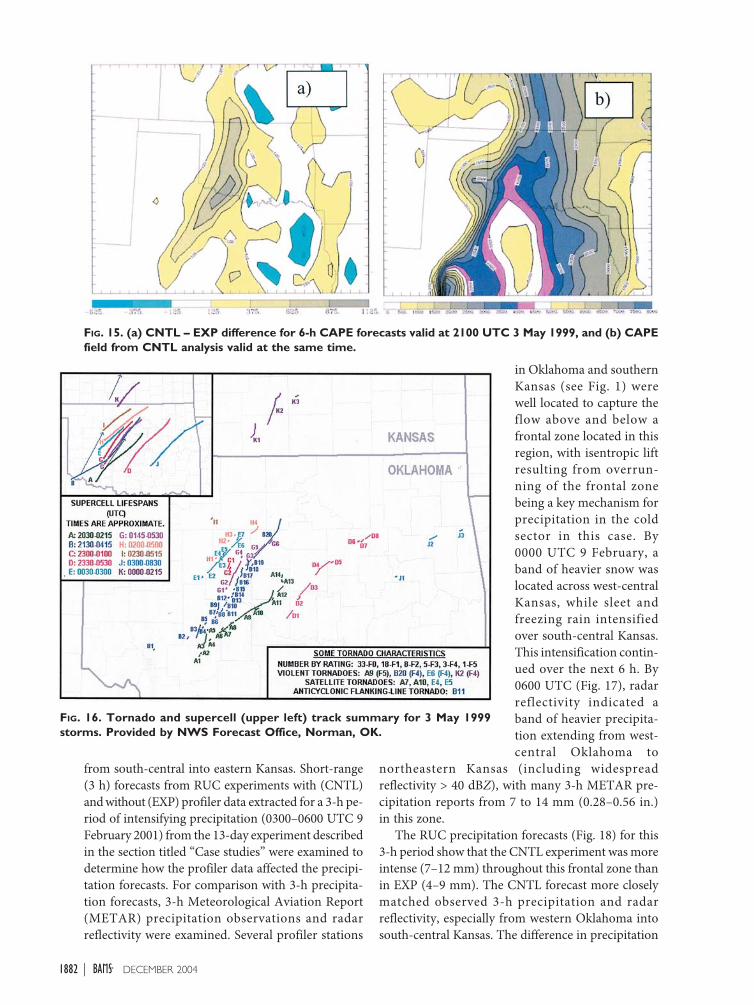
In addition to wind fields, forecasts of convectiveavailable potential energy (CAPE; an important pa-rameter indicating instability available to fuel con-vective storm development) derived from the RUCwere also examined from the CNTL and EXP experi-ments. (CAPE is calculated here with averaging ofpotential temperature and water vapor mixing ratioin the lowest 40 hPa.) Figure 15a shows the differ-ence between CNTL and EXP 6-h CAPE forecastsvalid at 2100 UTC 3 May 1999. Observed CAPE val-ues (Fig. 15b, CNTL analysis) are generally large(> 4000 J kg-1) in the area where the first stormsformed (see supercell track summary, Fig. 16, upper-left inset) in southwestern Oklahoma. The increase

in CAPE values (by ~1000 J kg-1) in this area in theCNTL run is primarily the result of an improved lo-cation of the axis of maximum CAPE (i.e., a reduc-tion in the phase error). The CAPE forecast improve-ment from the assimilation of profiler data waslargely related to an enhanced southeasterly flow ofmoisture (see Benjamin et al. 2004c, their Fig. S3)into the area of convective initiation and a westwardshift of dryline position. Both changes agree moreclosely with the observations.

Severe snow and ice storm of 9 February 2001. The20-km RUC was also used to examine the impact ofprofiler data for a winter storm that brought a vari-ety of weather to the U.S. southern plains on 8–9 February 2001, including heavy sleet and freezing rain

FIG. 14. The 6-h forecasts of 300-hPa wind (m s-----1) for (a) CNTL and (b) EXP initialized at 1800 UTC 3May 1999 and valid at 0000 UTC 4 May 1999. (c) Verifying (CNTL) analysis at 0000 UTC 4 May 1999,and (d) CNTL – EXP vector difference between 6-h forecasts.

1882 DECEMBER 2004|

from south-central into eastern Kansas. Short-range(3 h) forecasts from RUC experiments with (CNTL)and without (EXP) profiler data extracted for a 3-h pe-riod of intensifying precipitation (0300–0600 UTC 9February 2001) from the 13-day experiment describedin the section titled “Case studies” were examined todetermine how the profiler data affected the precipi-tation forecasts. For comparison with 3-h precipita-tion forecasts, 3-h Meteorological Aviation Report(METAR) precipitation observations and radarreflectivity were examined. Several profiler stations

in Oklahoma and southernKansas (see Fig. 1) werewell located to capture theflow above and below afrontal zone located in thisregion, with isentropic liftresulting from overrun-ning of the frontal zonebeing a key mechanism forprecipitation in the coldsector in this case. By0000 UTC 9 February, aband of heavier snow waslocated across west-centralKansas, while sleet andfreezing rain intensifiedover south-central Kansas.This intensification contin-ued over the next 6 h. By0600 UTC (Fig. 17), radarreflectivity indicated aband of heavier precipita-tion extending from west-central Oklahoma to

northeastern Kansas (including widespreadreflectivity > 40 dBZ), with many 3-h METAR pre-cipitation reports from 7 to 14 mm (0.28–0.56 in.)in this zone.

The RUC precipitation forecasts (Fig. 18) for this3-h period show that the CNTL experiment was moreintense (7–12 mm) throughout this frontal zone thanin EXP (4–9 mm). The CNTL forecast more closelymatched observed 3-h precipitation and radarreflectivity, especially from western Oklahoma intosouth-central Kansas. The difference in precipitation

FIG. 15. (a) CNTL – EXP difference for 6-h CAPE forecasts valid at 2100 UTC 3 May 1999, and (b) CAPEfield from CNTL analysis valid at the same time.

FIG. 16. Tornado and supercell (upper left) track summary for 3 May 1999storms. Provided by NWS Forecast Office, Norman, OK.


between the two experimentswas apparently related to thelower-tropospheric frontalposition and slope. A three-dimensional analysis of windflow responsible for these dif-ferences in precipitation, in-cluding comparisons of verti-cal cross sections of horizontaland vertical velocity and hy-drometeors, is presented inBenjamin et al. (2004c).

DISCUSSION AND CON-CLUSIONS. The importanceof data from the wind profilernetwork for forecasting in theUnited States has been docu-mented through data denial ex-periments with the RUC for a13-day period from February2001, three severe storm casestudies [3 May 1999, 9 February2001, and 8 May 2003 (seeonline supplement)], and asummary of the use of profilerdata within the NationalWeather Service. Verificationstatistics from the RUC profilerdata denial experiments shownin this paper demonstrate thatprofiler data contribute sig-nificantly to the reduction of

FIG. 18. Forecast 3-h precipitation (mm) for 0300–0600 UTC 9 Feb 2001 from (left) CNTL and (right)EXP forecasts initialized at 0300 UTC.

FIG. 17. Radar reflectivity (0.5∞∞∞∞∞ elevation scan, dBZ color scale shown at bot-tom) valid at 0600 UTC 9 Feb 2001 and METAR precipitation (in.) totalsfor 3-h period ending 0600 UTC. (From AWIPS.)

1884 DECEMBER 2004|

USE OF PROFILERS BY OPERATIONAL FORECASTERSWind profiler data are used regularly by NWS forecasters. Forecasters typically use a time-series display ofhourly profiler winds and also display overlays of profiler winds on satellite and/or radar images to betterdiscern mesoscale detail. In addition, profiler data are often used to help verify analyses and short-rangeforecasts from the models, enabling forecasters to judge the reliability, in real time, of the model guidance.NPN profilers are located near many Weather Forecast Offices (WFOs) in the NWS Central and South-ern Regions. (Also, boundary layer profilers located near each coast, not used in NWP tests describedhere, are used by the NWS Western and Eastern Regions). In 2002, the NWS Southern Region ScientificServices Division conducted a survey for WFOs within the NPN area to inquire how the profiler data areused in operations. Forecasters noted that they use profiler data for synoptic analysis, evaluation of modelguidance, mesoscale analysis, discerning short-term changes, checking the prestorm environment, moni-toring evolving upper-level jet streaks, and for LLJ detection and monitoring moisture advection with theLLJ. Forecasters described more specific instances in which profiler data were used, and some of these aregiven below:

· Topeka and Wichita (Kansas) WFOs: Monitored a rapidly evolving low-level shear profile that resulted inconditions favoring supercells, which enabled the forecasters to be well prepared in anticipating the tornadooutbreak on 19 April 2000. (The Neodesha, Kansas, profiler showed a vertical speed–directional shear profiledeveloping rapidly over a 3–6-h time period that was ideal for tornadic storms. Mesoscale data, includingprofilers, were used to put out an accurate and specific nowcast about exactly where severe convection woulddevelop in the next 1-h period.)

· Amarillo (Texas) WFO:

· Forecast high wind events by monitoring strong above-surface winds in the Texas and OklahomaPanhandles;

· Forecast cold air fronts through high-frequency monitoring of depth and strength of cold-air surge,which is possible only with profiler data;

· Monitor low-level jets and low-level wind shear profiles important for forecasting thunderstorm outbreaks and possible rotating storms and tornadoes.

· Topeka (Kansas) WFO: Ended a winter weather warning. (Profiler data confirmed that placement of anupper-level low in the models was incorrect, and the warning was cancelled much sooner than it otherwisewould have been.)

· Albuquerque (New Mexico) WFO: Specialized weather forecasting for fires near Albuquerque. (Windobservations from the Tucumcari profiler helped forecasters to accurately predict a midnight wind surgethat led to a fire blowup. Fire fighters were, therefore, prepared and able to contain the fire duringintensification.)

While the 3 May 1999 case was a dramatic example of profiler data use at the NOAA Storm PredictionCenter (see the beginning of this article), SPC forecasters often use profiler data on an hourly basis. Theimpacts/uses of profiler data at the SPC are summarized below:

· Needed to reliably diagnose changes in vertical wind shear at lower levels (< 3 km above ground level) as wellas through a deep layer (through 6 km AGL), both critical to determining potential tornado severity;

· Used to better determine storm motion, critical in distinguishing stationary thunderstorms that produce flood-ing from fast-moving thunderstorms that produce severe weather;

· Used to better determine storm relative flows and, consequently, the character of supercells [heavy precipi-tation (HP) versus classic];

· Critical for monitoring the low-level jet life cycle, an important factor in mesoscale convective system (MCS)development and, therefore, the threat for flooding and/or severe weather; and

· Unique in providing high-frequency full-tropospheric winds compared with radiosonde and VAD data. (WhileDoppler radar-derived VAD winds also provide a high frequency, they cannot monitor deeper-layer verticalwind shear, critical information for SPC. The SPC has added use of the 6-min profiler data since 2000 tobetter monitor conditions with rapidly evolving severe weather.)

[The material presented in the introduction and this sidebar were contributed by P. Browning of the NWS and S.Weiss of the NCEP Storm Prediction Center.]


the overall error in short-range wind forecasts overthe central United States for this February 2001 testperiod. Forecast errors for height, relative humidity,and temperature were also reduced by 5%–15% av-eraged over vertical levels. This contribution fromprofiler data is above and beyond the contributionsto initial conditions provided by complementary ob-servations from ACARS aircraft, VAD, and surfacestations. A significant contribution from profiler datato improved short-range (3 h) forecast accuracy of12%–28% at all mandatory levels from 850-150 hPawas shown from the RUC experiments for the 13-daytest period. Moreover, a substantial reduction of windforecast error (~25%) was shown to occur even atnear-tropopause jet levels for forecasts initiated atnight from the assimilation of profiler data.

Comparisons were made between experiments inwhich profiler data were withheld and a secondexperiment in which all aircraft data were withheld.The complementary nature of the two types ofobservations contributing to a composite high-frequency observing system over the United Stateswas evident, with profiler observations contributingmore to improvement through the middle and lowertroposphere, and aircraft observations contributingmore strongly at near-tropopause jet levels. The pic-ture is actually more complex, with aircraft ascent/descent data adding full-tropospheric profiles ofwinds and temperature and profilers contributinghigh-frequency jet-level wind observations at night,both adding further accuracy to short-rangeforecasts. Benjamin et al. (2004a), in a detailed de-scription of the RUC and the performance of itsassimilation–forecast system, show the effectivenessof the RUC in using high-frequency observationsover the United States to provide improved skill inshort-range wind forecasts down to as near term asa 1-h forecast. These accurate short-range forecastsare critical for a variety of users, including aviation,severe weather forecasting, the energy industry,spaceflight operations, and homeland securityconcerns. Without question, it is the combined ef-fect of the profiler–aircraft composite observing sys-tem that is most responsible for this strong perfor-mance in RUC short-range wind forecasts over theUnited States.

Profiler observations fill gaps in the ACARS air-craft observing system, with automated, continuousprofiles 24 h day-1, with no variations over the timeof day or the day of the week (package air carriersoperate on a much-reduced schedule over weekends).Profiler data are available (or could be) when aircraftdata may be more drastically curtailed, owing to na-

tional security (e.g., 11–13 September 2001) or severeweather events such as the East Coast snowstorm of15–17 February 2003. Profiler observations also allowimproved quality control of other observations fromaircraft, radiosonde, radar, or satellite.

Although the average statistical NWP impact re-sults are compelling evidence that the profiler dataadd value to short-range (0–6 h) NWP forecasts, thevalue ranges from negligible, often on days with be-nign weather, to much higher, usually on days withmore difficult forecasts and active weather. This day-to-day difference was evident in breakdowns ofprofiler impact statistics to individual days and to peakerror events. These breakdowns were made to accom-pany the cumulative statistics that generally mask thestronger impact that occurs when there is activeweather and a more accurate forecast is mostimportant.

Detailed case studies were carried out using theRUC assimilation cycle and forecast model with andwithout profiler data for three severe weather cases.A fairly significant positive impact was demonstratedfor the Oklahoma tornado outbreak cases of 3 May1999 and 8 May 2003. Wind data from the profilersresulted in an improvement in the forecast CAPE,shear, and precipitation forecasts valid at or near thetime of the storm development. In the 1999 case, theCAPE forecast improvement from assimilation ofprofiler data was largely related to an enhanced south-easterly flow of moisture into the area of convectiveinitiation and a westward shift of dryline position.Assimilation of profiler data for the 8–9 February 2001snow and ice storm case study resulted in a betterforecast of the ascent of the lower-level southerly flowoverrunning a strong cold front, resulting in stron-ger and broader upward motion. The outcome of as-similating profiler data in this case was a more accu-rate RUC precipitation forecast in an area ofsignificant sleet and snow in Oklahoma and Kansasnorth of the surface front.

As summarized in this paper, profiler data arewidely used and have become an important part of theforecast preparation process in the National WeatherService. Clearly, the utility of NPN data to local fore-cast offices is greatest for short-term forecasts andwarnings, reflecting the unique high time resolutionfrom profilers. The NPN is capable of providing datawith time resolution as high as 6 min, and forecastersin the NWS Central Region have only recently begunto access the 6-min data routinely. Early indicationsare that the utility of profiler data in critical short-fuse-warning situations is even further enhanced bythe 6-min data.

1886 DECEMBER 2004|

Profiler data are the only full-tropospheric winddata available on a continuous basis over the UnitedStates and, as discussed above, could possibly be theonly such data that would be available during extremeweather events or a national security event that wouldground commercial aircraft. Profilers also routinelyprovide full-tropospheric wind observations in con-ditions of full cloud cover that cannot be made fromany current or planned satellite system.

The critical improvements provided to short-rangemodel forecasts and subjective forecast preparationfrom wind profiler data, as documented in this paper,have been available only over the central United Statesand, to a lesser extent, downstream over the easternUnited States. The NWS Service Assessment Reportfor the 3 May 1999 tornado case (NWS 1999) recom-mended full operational support for the existingprofiler network. These benefits for forecast accuracyand reliability could be extended nationwide by imple-mentation of a national profiler network, although thisneeds to be the subject of a cost–benefit analysis. Asdescribed earlier, the interests that would obtain a na-tional-scale benefit from such a profiler network in-clude not only severe weather forecasting, but alsoaviation, energy, space flight, and homeland security.

ACKNOWLEDGMENTS. We thank Tom Schlatter,Nita Fullerton, and Margot Ackley of FSL for their reviewsof this manuscript and Randy Collander and Brian Jamisonfor contributions to graphics. Dan Smith and Pete Brown-ing of the Scientific Services Divisions in the NWS South-ern and Central Regions, respectively, and Steve Weiss ofthe NCEP Storm Prediction Center contributed the mate-rial presented in the introduction and the sidebar.

REFERENCESBenjamin, S. G., and Coauthors, 2002: RUC20—The

20-km version of the Rapid Update Cycle. NWSTechnical Bulletin 490, 30 pp. [Available online athttp://ruc.fsl.noaa.gov.]

——, D. Devenyi, S. S. Weygandt, and G. S. Manikin,2003: The RUC 3D variational analysis (and post-processing modifications). NOAA Tech. Memo.OAR FSL-29, Forecast Systems Laboratory, Boulder,CO, 18 pp.

——, and Coauthors, 2004a: An hourly assimilation/fore-cast cycle: The RUC. Mon. Wea. Rev., 132, 495–518.

——, G. A. Grell, J. M. Brown, T. G. Smirnova, and R.Bleck, 2004b: Mesoscale weather prediction with theRUC hybrid isentropic/terrain-following coordinatemodel. Mon. Wea. Rev., 132, 473–494.

——, B. E. Schwartz, E. J. Szoke, and S. E. Koch, 2004c:The value of wind profiler data in U.S. weather fore-casting: Case studies. Bull. Amer. Meteor. Soc., 85,doi:10.1175/BAMS-84-11-Benjamin.

Bouttier, F., 2001: The use of profiler data at ECMWF.Meteor. Z., 10, 497–510.

Devenyi, D., and S. G. Benjamin, 2003: A variationalassimilation technique in a hybrid isentropic-sigmacoordinate. Meteor. Atmos. Phys., 82, 245–257.

Edwards, R., S. F. Corfidi, R. L. Thompson, J. S. Evans,J. P. Craven, J. P. Racy, D. W. McCarthy, and M. D.Vescio, 2002: Storm Prediction Center forecasting is-sues related to the 3 May 1999 tornado outbreak.Wea. Forecasting, 17, 544–558.

Graham, R., J, S. R. Anderson, and M. J. Bader, 2000: Therelative utility of current observations systems to glo-bal-scale NWP forecasts. Quart. J. Roy. Meteor. Soc.,126, 2435–2460.

Martner, B. E., and Coauthors, 1993: An evaluation ofwind profiler, RASS, and microwave radiometer per-formance. Bull. Amer. Meteor. Soc., 74, 599–614.

Moninger, W. R., R. D. Mamrosh, and P. M. Pauley,2003: Automated meteorological reports from com-mercial aircraft. Bull. Amer. Meteor. Soc., 84, 203–216.

Morris, D. A., K. C. Crawford, K. A. Kloesel, andG. Kitch, 2002: OK-FIRST: An example of success-ful collaboration between the meteorological andemergency response communities on 3 May 1999.Wea. Forecasting, 17, 567–576.

National Weather Service, 1999: Oklahoma/southernKansas tornado outbreak of May 3, 1999. U.S. De-partment of Commerce Service Assessment, NOAA,51 pp. [Available from National Weather Service,1325 East-West Highway, W/OS52, Silver Spring,MD 20910, and online at ftp://ftp.nws.noaa.gov/om/assessments/ok-ks/report7.pdf.]

Thompson, R. L., and R. Edwards, 2000: An overviewof environmental conditions and forecast implica-tions of the 3 May 1999 tornado outbreak. Wea. Fore-casting, 15, 682–699.

van de Kamp, D. W., 1993: Current status and recentimprovements to the Wind Profiler DemonstrationNetwork. Preprints, 26th Int. Conf. on Radar Meteo-rology, Norman, OK, Amer. Meteor. Soc., 552–554.

Weber, B. L., and Coauthors, 1990: Preliminary evalua-tion of the first NOAA demonstration networkprofiler. J. Atmos. Oceanic Technol., 7, 909–918.

Zapotocny, T. H., W. P. Menzel, J. P. Nelson, and J. A.Jung, 2002: An impact study of five remotely sensedand five in situ data types in the Eta Data Assimila-tion System. Wea. Forecasting, 17, 263–285.

Documents

THE VALUE OF WIND PROFILER DATA IN U.S. WEATHER …