The variational solution of electric and magnetic circuits by A. A. F? Gibson and B. M. Dillon

Voltage and current distributions in electric circuits comply with a stationarypower condition. A n alternative circuit analysis technique can be dm'ved3om this property The unknowns can be varied until the power consumption of the circuit is calculated to be unchanging. A t this point the voltages and currentr are at their true solution. This variational approach to cimit analysis has been generally ovwlooked. No doubt this is due to the suJciency of conventional circuit analysis techniques. H o w a closer examination ofthe variational approach reveals a straigh$fOnuard analytic procedure with unfiing properties and graphically illustrated solutions. Thesefeatures provide new educational opportunities and insight. As a research tool the variational approach ofen a un$ed method ofsolvingproblems which includefields and deviies. The application to nonlinear circuits is also ofcurrent interest. A n introductory sttp-by-step guide to the variational procedurefor electric and magnetic networks is described in this article.

Introduction

s an engineering analysis tool, the variational approach is well established and has a solid foundation in both physics and A mathematics'. It is universally used with

numerical techniques and is accredited for its versatility, physical interpretation and elegance of formation. With variational methods the unique solution of an engineering problem is found via the stationary point of a suitable energy or power expression. Starting with a postulated solution the behaviour of energy is examined as the postulated solution is varied. An invarying energy quantiry, or stationary point, indicates a true solution. In the early days, this was done graphically; now, computers can do these numerical experiments very &ciently and accurately.

Variational methods are extended here to examine the behaviour of electric and magnetic circuits. In comparison to conventional circuit analysis methods the stationary power technique offers a simphfied formulation, a method of solution for nonlinear devices and relation to a universal principal*,'. This approach is also consistent with the variational/ '

finite-element method widely used for dstributed field problems. From an educational viewpoint the stationary solution of circuits provides a very descriptive introductory example to variational methods. The use of dfferential calculus and graphical illustrations also provides new and useful teaching material.

A variational power equation for circuits can be constructed h m the instantaneous power of an electrical network. Either unknown nodal voltage values or branch currents are used as the unknown variables. As power is a scalar quantity there are no restrictions on current and voltage polarities. Each circuit branch element is represented by an entry into the characteristic power equation. With nonlinear devices the voltage/current characteristic has to be integrated to form a power expression. One equation describes the entire circuit and its stationary point coincides with the circuit's true solution. The formulation lends itselfto approximation techniques or can be solved rigorously using matrix methods.

The stationary power procedure for lumped element circuits is described here by having recourse to some simple steady-state circuits with DC and AC sources.

ENGINEERING SCIENCE AND EDUCATION JOURNAL FEBRUARY 1995

5

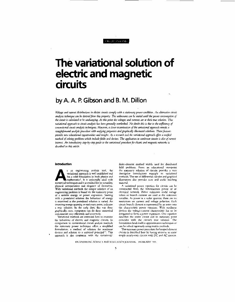
Characteristic power equations are formed for linear capacitive, resistive and Eeactive impedance circuits. A formal analytic procedure is developed and supplemented by graphical solutions. A nonlinear resistor problem is treated before considering a nonlinear mag- netic circuit. The approach described can be extended to evaluate harmonics in nodnear circuits and to produce the unified solution of lumped- element/distributed-field prob- lems’.

100 v

reference

Fig. 1. The potential? VI and Vz are unknown If VI and Vz are varied then the overall stored energy of the circuit wdl also vary In th s process there IS a unique solunon pair of VI and V2 which m m s e s the circuit’s stored energy The first step is to construct an energy charac- teristic equation for the circuit. In electromagnehcs this is called a funcnonal The energy stored by a capacitor, C, is a funcnon of

Minimum energy solution of capacitor circuits

Theoretical stumes in electrical engineering can either involve a Iltstributed-space or lumped-element circuits. In distributed problems electromagnetic fields and potentials are calculated. A simple class of Iltstributed problem is that of electrostatics, where electric charge is time stationary. The electric-field and voltage solution of a capacitor plate arrangement is one example. It is well known that in electrostatics the voltage solution in a distributed space corresponds to a minimum stored energy. Indeed this result i? routinely used in numerical techniques which rely on variational methods. In variational methods the unknowns of the problem are varied until the calculated value of a suitable energy expression is unchanging.

Electric lumped-element capacitor circuits also exhibit this minimum energy behaviour. Energy analysis in circuits is straightforward and therefore provides an excellent introduction to variational mer& methods. Consider the capacitor circuit illustrated in

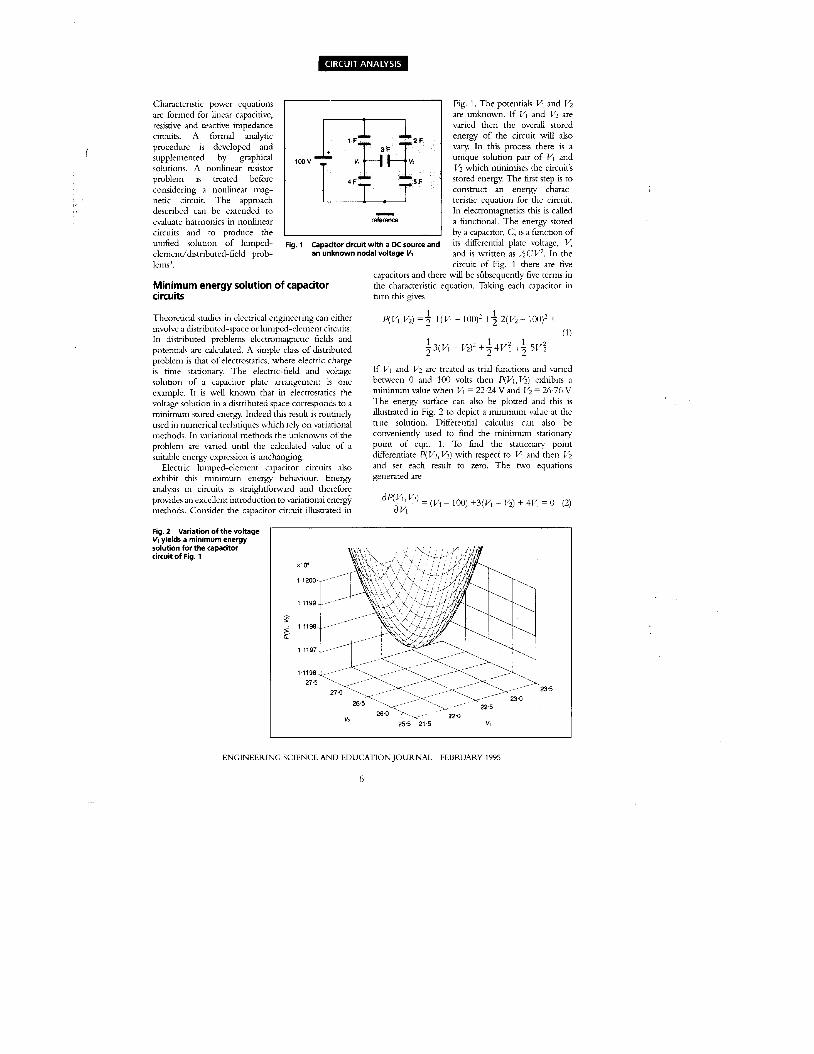
Fig. 2 Variation of the voltage VI yields a minimum energy solution for the capacitor circuit of Fig. 1

circuit of Fig. 1 there are five capacitors and there will be shbsequently five terms in the characteristic equation. Talang each capacitor in turn this gives

1 P(Vt,Vz) =z l ( K - loo)* ++ 2(&- loo)? +

If VI and V2 are treated as trial functions and varied between 0 and 100 volts then P(VI,V~) exhibits a minimum value when l4 = 22.24 V and V2 = 26.76 V The energy surface can also be plotted and this is dlustrated in Fig. 2 to depict a minimum value at the true solution. Differential calculus can also be conveniently used to find the minimum stationary point of eqn. 1. To find the stationary point differentiate P( V I , Ly2) with respect to VI and then V2 and set each result to zero. The two equations generated are

aP(Vl,Vr) - ~- aVl

(VI - 100) +3(K - Vz) + 4111 = 0 (2)

I 22 5 V,

255 21 5 V,

ENGINEERING SCIENCE ANI1 EIIUCATION JOURNAL FEBRUARY 1995

6

204 - 100) -3(K - V2) +5V2 = 0 (3) a q C; , v ~ ) - av2 . --

and these simultaneous equations have the solution given above. It is also instructive to examine the nature of the turning point using calculus. Forming the second order derivatives of eqn. 1 yields

(4)

(5)

which are both positive quantities and indicative of minimum turning points as illustrated in Fig. 2.

An advantage of demonstrating variational methods using circuits is that the result is easily corroborated using conventional circuit analysis techniques. The circuit of Fig. 1 can be solved in at least three other ways. Th6venin's theorem in conjunction with circuit reduction techniques is one approach. This method would however not work for a more complicated circuit arrangement, Another approach involves substituting an AC supply for the battery using capacitive reactances, and talung the solution as the linlit of zero frequency. A less obvious method would be to use the equation of continuity which describes the indestructibility of charge. Each approach identically generates the equations 2 and 3.

Variational solution of a resistor circuit

Purely resistive circuits also comply with the stationary power principle. The power dissipated in each resistor branch of a netuork can either be written in terms of

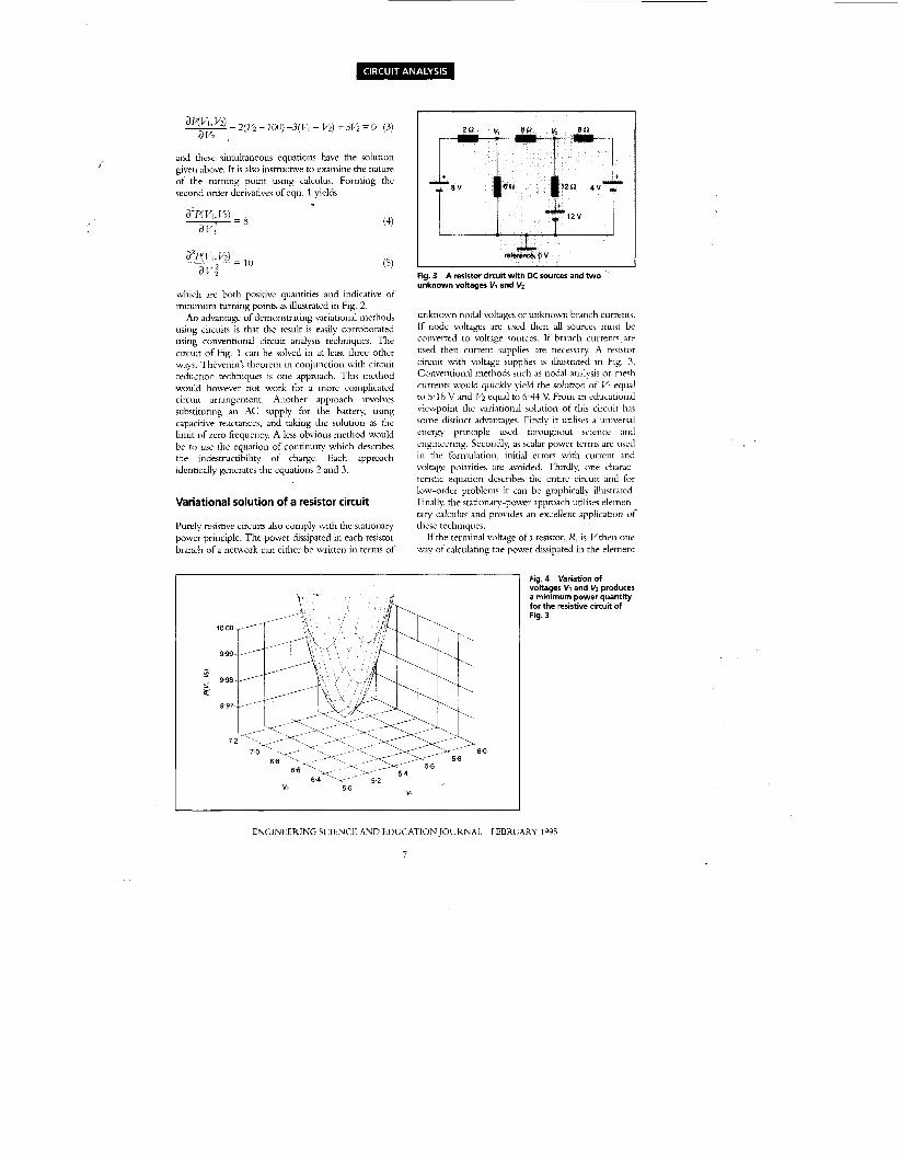
I Fig. 3 A resistor circuit with DC sources and two ' unknown voltages VI and VZ

unknown nodal voltages or unknown branch currents. If node voltages are used then all sources must be converted to voltage sources. If branch currents, are used then current supplies are necessary. A resistor circuit with voltage supplies is illustrated in Fig. 3. Conventional methods such as nodal analysis or nieuh currents would quickly yield the solution of VI equal to 5.18 V and V2 equal to 6.44 V. From an educational viewpoint the variational solution of this circuit has some distinct advantages. Firstly it utilises a universal energy principle used throughout science and engineering. Secondly, as scalar power terms are used in the formulation, initial errors with current and voltage polarities are avoided. Thirdly, one charac- teristic equation describes the entire circuit and for low-order problems it can be graphically illustrated. Finally, the stationary-power approach udises elemen- tary calculus and provides an excellent application of these techniques.

If the ternunal voltage of a resistor, R, i5 Vthen one way of calculating the power dissipated in the element

io00

999

- : 998 r

9 97

7 6 0

V, 5 0 V,

Fig. 4 Variation of voltages VI and VZ produces a minimum power quantity for the resistive circuit of Fig. 3

ENGINEERING SCIENCE AND EDUCATION JOURNAL FEBRUARY 1995

7

I J Fig. 5 An AC source circuit with reactive impedances and one unknown complex nodal voltage VI

i5 to form the equation V'/R. Using this equation and taking each branch resistance in turn, the power characteristic equation &'(VI, V2) of the circuit can be constructed. There are five branch resistances, therefore there are five contributing terms to this equation:

The voltages I.; and V? can be varied as trial functions and the power can be calculated for each point. This variational process is illustrated in Fig. 4, where a minimum is illustrated at the true solution given earlier. Alternatively, the minimum power poiut can be found using differential calculus. Differentiate P(V1, V') with respect to the unknowns VI and V2 and set each result to zero to find the stationary point. The two

simultaneous equations generated are as follows:

These equations are exactly those which are produced when using conventional nodal analysis and have a solution of VI equal to 5.18 V and V2 equal to 6.44 V. The second order derivatives of eqn. 6 yield positive quantities which imply a minimum turning point, as dustrated in Fig. 4.

Variational solution of an AC circuit

Electrical circuits with AC signal sources and reactive elements are described in terms of impedances rather than pure resistances. The unknown nodal voltages or branch currents in the circuit become complex quantities describing both magnitude and phase. A suitable variational expression for this class of problem is deduced fiom the apparent power quantity which can be written in t e rm ofthe adjacent unknown nodal voltages. The characteristic equation for the circuit is constructed from the linear addition ofapparent power consumed by each branch. There are three impedance branches in the circuit of Fig. 5 and therefore there are three entries in the characteristic equation. The result is written in terms of VI as

(9)

The real and imaginary parts of the complex variable K mav be varied and the value of auuarent Dower

-14

16 -22

* I I

calculated. Fig. 6 illustrates this construction in the vicinity of the stationary point. This point coincides with the true solution for VI. It is of note that the complex functional yields a stationary saddle point. Analytically the stationary point is determined from the first variation of eqn. 9. This yields the following equation:

Fig. 6 For the AC circuit of Fig. 5 the variation of the real and imaginary parts of VI yields a stationaly saddle point

which has the solution of VI = 12.3-j18.5.

ENGINEERING SCIENCE AND EDUCATION JOURNAL FEBRUARY 1995

8

Variational solution of a nonlinear resistor circuit

Nonlinear passive components which are characterised by a single-valued current/voltage relationship also obey the stationary power principle’. The contribution of each element in the nodnear circuit to the charalteristic power equation is evaluated using integral terms. For example, the power dissipated in a nonlinear resistor connected between nodes VI and V2 is

19.7-

19.5-

19.3

- 5 c

19.1

18.9

P = jLyI(V)dV

-

-

-

Once the characteristic power equation has been formed, the variational solution procedure is identical to that for linear D C circuits.

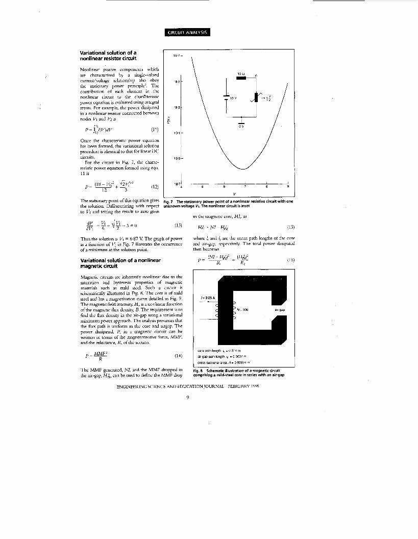
For the circuit in Fig. 7, the charac- teristic power equation formed using eqn. 11 is

The stationary point ofthis equation gives Fig. 7 The stationary power point of a nonlinear resistive circuit with one the solution. Differentiating with respect unknown voltage V,. The nonlinear circuit is inset to VI and setting the results to zero gives

Thus the solution is VI = 6.87 V The graph of power as a function of VI in Fig. 7 illustrates the occurrence of a minimum at the solution point.

Variational solution of a nonlinear magnetic circuit

Magnetic circuits are inherently nonhear due to the saturation and hysteresis properties of magnetic materials such as mild steel. Such a circuit is schematically illustrated in Fig. 8. The core is of n d d steel and has a magnetisation curve detded in Fig. 9. The magnetic field intensity, H,, is a nonlinear function of the magnetic flux density, B. The requirement is to find the flux density in the air-gap using a variational minimum power approach. The analysis presumes that the flux path is uniform in the core and airgap. The power dlssipated, P, in a magnetic circuit can be written in t e rm of the magnetomotive force, MMF, and the reluctance, R, of the section:

- MMF2 R

The MMF generated, NI, and the MMF dropped in the air-gap, H&, can be used to define the MMF drop

in the magnenc core, HL, as

H,I, = rvr - H,I, (15)

where I, and are the mean path lengths of the core and air-gap, respectively. The total power hssipated then becomes

core path length, IC = 0314 m

air gap path length, ig = 0-0007 m

cross-sectional area, A = 0.00024 mi

Fig. 8 Schematic illustration of a magnetic circuit comprising a mild-steel core in series with an air-gap

ENGINEERING SCIENCE AND EDUCATION JOURNAL FEBRUARY 1995

9

I

H kNm

Fig. 9 Magnetisation characteristics of a mild-steel core

where the reluctances of the core, &, and gap, 4, are defined using the cross-sectional area, A, and flux density, B, as

Substituting eqns. 17 and 18 into 16 and using the relationship E = bHR in the air-gap, the power dlssipated in the magnetic circuit becomes

Eqn. 19 has two unknowns, H, and B, which are also related by the magnetisation curve of Fig. 9. Substituting an (H(, B) pair from Fig. 9 into eqn. 19 yields a scalar power quantity. This quantity varies with different (fi, B) pairs. It exhibits a minimum at the true solution. This variational process is illustrated in Fig. 10. A minimum quantity is clearly exhibited at a flux density of around 1.35 tesla. Conventional methods can be used to check this result by worlang backwards from the solution to the MMF eqn. 15.

Conclusion

Variational methods do not consist of solving a set of equations but in approximating to a trajectory or functional. Physically interpreted the method dlsplaces

2 0

1 5

8 1 0

0 5

0 I I I I I ,

0.6 0.8 1.0 1 2 1.4 1.6 1.8

B. tesla

Fig. 10 Stationary minimum power quantity illustrated at the true solution for the magnetic circuit

a system from its dynamic equilibrium position and examines the dlsplaced behaviour. In the application to electrical circuits the behaviour of a power functional is examined as the unknown voltages or currents are displaced. When the first variation is set to zero the unknowns are in the vicinity of their correct solution. This approach has been described by examining the behaviour of some linear and nonhear electric and magnetic circuits.

There are a number of new possibilities which arise from the application of variational methods to circuits. A unified electromagnetic field solver with a lumped- element device facility would be a useful proposition for applications which combine irregular geometries with resistors, capacitors etc. Additional information can be generated concerning the nature of a solution and its convergence. Confidence limits on convergence parameters may be of particular use in nodnear applications.

References

1 MIKHLIN, S. G.: ‘Variational methods in mathemancal physics’ (Macmillan, New York, 1964)

2 HAMMOND, E?: ‘Energy methods in electromagnetism’ (Oxford Science Publications, 1981)

3 GIBSON, A. A. E?, and DILLON, B. M.: ‘Variational solution of lumped element and rllstnbuted electrical circuits’, IEE Roc. Si., Mea. Tethnol., September 1994, 141, (5), pp.42H28

0 IEE: 1995

The authors are with the Department ofElectrical Engineering and Electronics, UMIST, PO Box 88, Manchester, M60 1QD. UK.

ENGINEERING SCIENCE AND EDUCATION JOURNAL FEBRUARY 1995

10