The Vasicek adjustment to beta estimates in the Capital ... · estimates in the Capital Asset Pricing Model . ... The Vasicek adjustment to beta estimates in the Capital Asset Pricing

Stephen Gray and Jason Hall, SFG Consulting Neil Diamond and Robert Brooks, Monash University

The Vasicek adjustment to beta estimates in the Capital Asset Pricing Model 17 June 2013

The Vasicek adjustment to beta estimates in the Capital Asset Pricing Model (17 June 2013)


Contents 1. Preparation of this report ........................................................................................... 1 2. Executive summary .................................................................................................... 2 3. Issue and evaluation approach ................................................................................... 4

3.1. A statistical correction ........................................................................................ 4 3.2. The statistical “prior” .......................................................................................... 4 3.3. Statistical rationale .............................................................................................. 5 3.4. Performance evaluation ...................................................................................... 6 3.5. Detailed methodology ......................................................................................... 7

4. Data ............................................................................................................................ 9 5. Relationship between expected returns and realised returns ................................... 12 6. Conclusion ............................................................................................................... 15 7. References ................................................................................................................ 16 8. Appendix .................................................................................................................. 17 9. Terms of reference and qualifications ...................................................................... 19



1

1. Preparation of this report

This report was prepared by Professor Stephen Gray, Dr Jason Hall, Professor Robert Brooks and

Dr Neil Diamond. Professor Gray, Dr Hall, Professor Brooks and Dr Diamond acknowledge that they

have read, understood and complied with the Federal Court of Australia’s Practice Note CM 7, Expert

Witnesses in Proceedings in the Federal Court of Australia. Professor Gray, Dr Hall, Professor Brooks

and Dr Diamond provide advice on cost of capital issues for a number of entities but have no current

or future potential conflicts.



2

2. Executive summary

Beta estimates for the Capital Asset Pricing Model (CAPM) can be obtained by applying ordinary

least squares (OLS) regression to the returns of firms in the same industry as the firm of interest and

returns on a diversified market portfolio. However, these OLS estimates are known to be subject to a

high degree of estimation error (Gray, Hall, Klease and McCrystal, 2009). Consequently, we consider

whether an easily-implemented econometric technique, the Vasicek (1973) adjustment, can mitigate

estimation error and thereby increase the reliability of beta (and ultimately cost of capital) estimates.

The Vasicek adjustment shifts the OLS beta estimate towards a prior expectation and the

magnitude of that shift is greater when the standard error of the OLS estimate is higher. That is, where

the OLS beta estimate is more precise it is given more weight, and when it is less precise it is given

less weight. In our case the prior expectation of beta is one because, prior to conducting the regression

analysis, we have no knowledge of whether the systematic risk of any given firm is above or below

average, according to the rationale set out below.

Suppose we know nothing at all about the firm of interest, nothing about capital structure,

industry, size, or competition.1 Our best estimate would be that this firm has a beta of one, because we

have no information whatsoever to determine whether it is a firm of above- or below-average

systematic risk. Now suppose we are told the firm is in a particular industry and that it is financed

with a specified amount of leverage. All else equal, leverage increases systematic risk, and different

industries could have different exposure to economic conditions (i.e., different asset betas). What we

cannot possibly know in advance is whether the combined impact of leverage and industry contributes

to the firm having above- or below-average systematic risk. The firm could be in a low risk industry

but have high leverage, or could be in a high risk industry but with low leverage. The reason we

cannot know in advance whether the firm is likely to be relatively high or low risk is because we have

not yet estimated beta for any similar firms. If we already knew the true beta for the average firm in

the same industry with the same leverage, we would not need to perform the estimation at all.2

This is why estimates provided by the major commercial data vendors such as Datastream and

Bloomberg adjust beta estimates towards a prior expectation of one. The estimates provided by

Datastream incorporate a very similar adjustment to the Vasicek adjustment, with a prior expectation

of one and the magnitude of adjustment contingent upon the standard error of the OLS beta estimate.

Estimates provided by Bloomberg place a one-third weight on a prior expectation of one and a two-

thirds weight on the OLS beta estimate.

1 That is, suppose you are given the task of providing your best estimate of the beta of a particular firm, without being told which firm it is. 2 That is, the task at hand is to select an appropriate beta value for the benchmark firm. The distribution of (re-levered) beta estimates for comparable firms can be used for that purpose. The goal is to construct the distribution of (re-levered) beta estimates for comparable firms. If we already knew that distribution somehow from our “prior” knowledge, there would be no need for any estimation at all.



3

We assess whether OLS and Vasicek-adjusted OLS estimates are able to predict stock returns

when incorporated into the CAPM. Our objective is to determine whether we can analyse historical

returns in order to make better predictions of future returns relative to just assuming that all stocks

will earn the market return.

Each month we compile beta estimates using returns information from all prior months.3 We then

form expected returns by incorporating these beta estimates into the CAPM, in which the risk free rate

is the yield on 10 year government bonds and the market risk premium is the excess market return

observed over the subsequent four weeks. In short, we ask, based upon the beta estimate and the

market return over the month what return would we expect the stock to earn over that month? In

performing this test we want to minimise the impact of random company- and industry-specific events

on realised returns. So in each month we form portfolios in the following manner. First, we partition

stocks into 10 industries according to the Industry Classification Benchmark (ICB) of FTSE. Second,

within each industry group we partition stocks into equal-sized cohorts of high, medium and low beta

stocks, formed on the basis of OLS beta estimates. We then aggregate the high beta stocks across the

10 industries, the medium beta stocks across the 10 industries and the low beta stocks across the 10

industries. This means that in each month we have three portfolios with the same industry

composition, so mitigate the impact that company- and industry-specific events will have on the

relative returns of each portfolio. We perform this analysis on two samples, a sample of 1,103 stocks

for which at least 10 years of returns are available for beta estimation and a sample of 2,585 stocks for

which at least 36 four-weekly returns are used in beta estimation (2.75 years of returns).

We find that expected returns formed from Vasicek-adjusted OLS estimates have more ability to

explain the variation in realised stock returns than OLS estimates. For the sample in which at least 10

years of returns are available for analysis, in a regression of realised portfolio returns on expected

returns the explanatory power is 57.78% as measured by the R-squared. In contrast, expected returns

derived from OLS beta estimates have an R-squared of 56.59%. This is a small improvement in

explanatory power, compared to assuming that all stocks have a beta of one. Under this naïve

assumption the R-squared is 54.54%. Furthermore, when estimates are compiled using shorter time

periods, OLS estimates perform worse than simply assuming all stocks have a beta estimate of one,

but Vasicek-adjusted OLS estimates have some explanatory power.

These results do not imply that Vasicek-adjusted OLS estimates are highly reliable and should

therefore be used in cost of capital estimation without consideration of other issues. The incremental

explanatory power is low. But we can conclude that Vasicek-adjusted OLS estimates are more reliable

measures of systematic risk than unadjusted OLS estimates.

3 Our returns are constructed over four weeks rather than every month, so each return is over the same time period, but we use the term monthly returns for convenience. There are 13.04 four-weekly returns per year, that is, 365.25 days ÷ 28 days = 13.04 four-weekly periods.



4

3. Issue and evaluation approach

3.1. A statistical correction

The issue at hand is the usefulness of alternative techniques for estimating systematic risk, to be

incorporated into the CAPM. We consider two estimation techniques which rely exclusively on the

analysis of historical stock returns. The first estimation technique is OLS regression of excess stock

returns on excess market returns. The second technique, the Vasicek adjustment, computes the beta

estimate as a weighted average of the OLS estimate and a prior or “null” expectation.

The Vasicek-adjusted OLS estimates we compute are a weighted average of the OLS estimate and

a beta estimate of one, the estimate for the average stock in the market. The idea behind these

estimates is that we cannot observe the true beta for any stock, all we can observe is a beta estimate

based upon a sample of returns. So if we observe a beta estimate that is well above or below that of

the average stock, there is some chance that the stock really does have systematic risk which is very

high or very low, and some chance that it has average risk and that we have observed the high or low

beta estimate purely by chance – as a result of estimation error. In particular, a very low beta estimate

is relatively more likely to have been affected by negative estimation error and a very high beta

estimate is relatively more likely to have been affected by positive estimation error – even if

estimation error is symmetric. This is explained in the context of the example that is set out in the

Appendix.

Vasicek (1973) also demonstrates that a beta estimate that is below one is more likely to have

been affected by negative estimation error. He also shows that the further a beta estimate is below

one, the greater the likely impact of negative estimation error. Consequently, if the OLS beta estimate

for a particular firm is below one, the best forecast of the true beta for that firm is something above

the OLS estimate. Vasicek (1973) demonstrated that the adjustment to eliminate the effect of

estimation error depends upon the standard error of the beta estimate. So the Vasicek-adjusted

estimate places some weight on the OLS estimate, and some weight on a prior estimate formed prior

to analysing the stock returns, and those weights depend on the standard error of the beta estimate.

3.2. The statistical “prior”

In the case at hand, the statistical prior estimate is one, which is (by definition) the true beta of the

average firm. Consequently, our Vasicek-adjusted beta estimates place some weight on the OLS beta

and some weight on the average or “null” beta estimate of one – where the relative weights depend

upon the statistical precision of the OLS estimate.

In our setting, the goal is to estimate the beta of the average firm in a particular industry. In other

settings, the goal is to estimate the beta of a specific individual firm. If the researcher already knows

the beta of the average firm in a particular industry, the Vasicek approach can be applied by adjusting

the OLS estimate for an individual firm towards the beta of the average firm in the industry. But this

is not at all relevant in our setting – if we knew the beta of the average firm in the industry, the task



5

would already be complete and no further analysis would be required. The whole point is that we

don’t know the beta of the average firm in the industry – that is what we are seeking to estimate. The

only quantitative a priori information that is available is that the beta of the average firm is one, by

definition.4

There are at least two data providers who compile beta estimates that are consistent with the

Vasicek approach (whereby raw OLS estimates are adjusted towards 1.0 based on the standard error

of the OLS estimate). The default estimates provided by Datastream are compiled using a Vasicek

adjustment, according to the technique described in Cunningham (1973). Bloomberg reports beta

estimates after applying a one-third weight to a prior estimate of one, and a two-thirds weight to the

OLS estimate.

3.3. Statistical rationale

Blume (1975) also documented mean reversion in OLS beta estimates, in that if we observe a low

beta estimate from sample returns in one period, we are likely to observe a higher beta estimate next

period, and that high beta estimates predict relatively lower beta estimates next period. Blume

speculated that one reason for this mean-reversion could be that over time the systematic risk of the

firm’s portfolio of assets approaches the systematic risk of the average firm in the market. But Blume

merely offered this as a potential explanation and did not test this conjecture. Vasicek demonstrated

that, even if there were no change whatsoever to the firm’s true systematic risk, we would observe

mean-reversion in beta estimates.

That is, there are two rationales for computing an adjusted beta. First, the true beta may revert

towards one over time as the firm takes on more projects with systematic risk which is about the same

as the average firm; or the firm changes its financing structure such that firms with high operating

leverage take on less financing leverage and vice versa. Under this rationale, having obtained a low

beta estimate this period, we would predict a higher beta estimate next period on the basis that the

firm will undertake actions that cause its true beta to revert towards one.

The second rationale is purely statistical, as set out in the example in the appendix. Under this

rationale, having observed a low beta estimate this period, we apply a statistical adjustment to correct

for statistical bias caused by estimation error. Note that under this rationale, the true beta does not

revert towards one over time at all – the adjustment is performed as a statistical correction only. As set

out in the appendix, the Vasicek correction is clearly a statistical adjustment to correct bias due to

4 In Vasicek’s (1973) paper he provides an example of the case in which the prior expectation is not equal to one, and refers to the case of a utility in which the prior expectation is 0.8 with a standard error of 0.3. There are two points to make with reference to this example. First, Vasicek was providing the reader with an example merely to describe the case in which the prior expectation is something different from one and elected to illustrate this point with a utility example. He was not making a comment about the actual beta estimates for utilities. Second, Vasicek was also illustrating the general case in which a prior expectation can only be formed using information other than the data and technique used in beta estimation. This means that it is not appropriate to use the same data and technique to form the prior expectation and conduct the regression analysis.



6

estimation error, as it is based on Bayes’ Rule. Such a correction clearly has nothing to do with true

betas mean reverting over time.

The Australian Energy Regulator (AER, 2009) has previously not adopted the Vasicek adjustment

for the small sample of Australian-listed stocks it typically considers. The AER’s primary reason for

the rejection of any adjustment towards one is that the benchmark firm does not diversify or change

its capital structure over time, so would not be expected to have a true beta that reverts towards one.

We agree that the mean reversion rationale is unlikely to apply to the benchmark firm. This is our

motivation for using the Vasicek correction; it mitigates the statistical bias caused by estimation error

– based on Bayes’ Rule, as set out in the example in the appendix.

The AER has also noted that the actual sample firms generally had beta estimates below one and

so adopting a prior estimate of one was likely to lead to an upwards bias in the results (p.297).5 It

contends that because it has used a sample of stocks in the same industry it has accounted for the

potential estimation error in OLS beta estimates.

The problem is that the AER has not addressed the real possibility that a very low OLS estimate is

more likely to understate risk than to overstate risk, and a very high OLS estimate is more likely to

overstate risk than understate risk. The use of a sample of firms in the same industry does not account

for this. If an event occurs which affects the industry in general, this can lead to an increase or

decrease in the beta estimates across the industry. For example, if there is takeover activity in a

particular industry when the market is performing well, the beta estimates for those firms will increase

because industry returns are high when the market returns are high; if there is a downturn in

commodity prices when the market is performing well the beta estimates for resources companies will

decrease because industry returns are low when the market is performing well.

3.4. Performance evaluation

To evaluate the performance of OLS beta estimates and Vasicek-adjusted OLS beta estimates we

tested the extent to which expected returns formed on the basis of a particular beta estimate are able to

predict future stock returns – relative to expected returns that are formed on the basis that all stocks

have a beta of one (the beta of the average firm). In other words, an estimate will be relatively more

reliable if it allows us to predict stock returns better than simply assuming all stocks have a beta of

one. Testing estimates against this criteria is generally challenging, because of the volatility of stock

returns. However, we have compiled a sample size that is sufficiently large to enable us to detect

improvements in the reliability of the estimates relative to a statistical prior assumption that beta is

equal to one.

We measure this improvement by comparing the R-squared from the regression of expected

returns on actual stock returns – for portfolios formed from high, medium and low beta stocks.

5 The first comment was made with respect to the Blume adjustment (in which a constant weight is applied to a prior expectation instead of a weight which varies according to the standard error of the beta estimate) but this same rationale was used to reject the use of the Vasicek adjustment.



7

Expected returns are formed by observing actual market returns and actual risk-free rates and asking,

“Given the beta estimate and the actual return earned by the market, what is the return we would

expect to earn on the portfolio?” This expected return appears on the right hand side of the regression

and the realised return for the portfolio appears on the left hand side. The reason we form portfolios

for this analysis is to eliminate the noise from individual stock returns as much as possible.

The R-squared from the regression measures how much the variation in realised returns can be

explained by expected returns formed on the basis of a particular estimate of beta. An R-squared of

100 per cent would imply that the CAPM (based on the particular estimate of beta from historic return

observations) could predict future returns with certainty. An R-squared of 50 per cent means that the

CAPM (based on the particular estimate of beta) can explain half of the variation in actual stock

returns, with the remaining variation in stock returns being explained by risk factors not encapsulated

by the CAPM.

We find that Vasicek-adjusted OLS estimates are better able to explain realised returns than are

raw OLS estimates. While there is only a small improvement in explanatory power over the

assumption that all stocks have beta equal to one, the evidence shows that Vasicek-adjusted OLS

estimates are relatively more reliable.

3.5. Detailed methodology

We first compute OLS beta estimates according to the following equation. Every four weeks we

compile beta estimates using returns information from all prior periods.6 In OLS regression, the

intercept (α) and coefficient on excess market returns (β) is determined in order to minimize the sum

of squared errors.

where:

ri,t, rm,t and rf,t represent the return on stock i, the return on the equity market and the risk free rate,

respectively in period t; and

εi,t represents the error term for stock i during period t.

Vasicek-adjusted OLS estimates place some weight on a statistical “prior,” and some weight on

the OLS estimate, with weights determined by the standard error of the OLS estimates. As explained

above, we adopt a beta of one as our statistical prior. This beta value is equal to the systematic risk of

the average firm (by definition). We compute Vasicek-adjusted OLS estimates for stock i (βiVAS)

according to the following equation, in which the standard error of our statistical prior E[std err] is

estimated as the standard deviation of OLS beta estimates in that month:7

6 Our returns are constructed over four weeks rather than every month, so each return is computed over the same time period. 7 This is likely to overstate the standard error of the prior estimate and therefore likely to understate the extent to which the OLS estimates should be shifted towards one on the basis of the Vasicek adjustment. The reason it is likely to overstate the standard error of the prior estimate is because the standard deviation of OLS estimates



8

Having compiled beta estimates under both techniques, we then evaluate whether expected returns

formed with respect to these estimates are able to explain the variation in realised returns. We then

form expected returns by incorporating these beta estimates into the CAPM, in which the risk free rate

is the yield on 10-year government bonds and the market risk premium is the excess market return

observed over the subsequent four weeks. In short, we ask, based upon the beta estimate and the

market return over the month what return would we expect the stock to earn over that month. For

example, if the beta estimate was 0.8, government bond yields were 0.5% and the market return was

2.0% we would expect the stock to earn returns of 1.7%, computed as rf + β × (rm – rf) = 0.005 + 0.8 ×

(0.020 – 0.005) = 0.005 + 0.8 × 0.015 = 0.005 + 0.012 = 1.7%.

In performing this test we seek to minimise the impact of random company- and industry-specific

events on realised returns by forming portfolios in the following manner. First, we partition stocks

into 10 industries according to the Industry Classification Benchmark (ICB) of FTSE. Second, within

each industry group we partition stocks into equal-sized cohorts of high, medium and low beta stocks,

formed on the basis of OLS beta estimates. We then aggregate the high beta stocks across the 10

industries, the medium beta stocks across the 10 industries and the low beta stocks across the 10

industries. This means that in each month we have three portfolios with the same industry

composition, so mitigate the impact that company- and industry-specific events will have on the

relative returns of each portfolio. We perform this analysis on two samples. We consider a sample for

which at least 131 four-weekly returns are used in beta estimation (10 years of returns) and a sample

for which at least 36 four-weekly returns are used in beta estimation (2.75 years of returns).

reflects both the dispersion of true betas and the estimation error inherent in the OLS estimates. So the standard deviation of beta estimates will be wider than the standard deviation of true betas.



9

4. Data

We compiled beta estimates for 2,585 Australian-listed stocks using returns computed from 2

January 1976 to 4 May 2012. The returns interval is four weeks, computed using Friday closing

prices, so there are 474 four-week periods. The market index is the All Ordinaries Accumulation

Index from 1 May 1992 and the Datastream Australia Total Market Index prior to this date. The

estimate of the risk free rate is the yield to maturity on 10-year Australian government bonds as

reported by the Reserve Bank of Australia, converted to a 28 day yield. We excluded firms with less

than 36 four-weekly returns observations and individual observations with a four-weekly return of

more than 200%.8

The beta estimates at each date comprise all available returns information prior to that date. In our

test of the relationship between expected returns and realised returns, we perform the analysis using

two samples. One sample requires at least 131 returns observations to be used in beta estimation, and

the other requires at least 36 returns observations to be used. There are two reasons we evaluate the

results over two time periods. First, we want to document whether the results differ if shorter or

longer time periods are used in beta estimation. Second, in practice, beta estimates are often compiled

over different time periods, either because there is limited data actually available or because the

analyst determines that a particular time period will provide more relevant information.

The selection of a minimum period of 10 years for the first sample aligns with the period from

January 2002 to the present day. In prior analysis, the AER has compiled beta estimates which

exclude the technology bubble which the AER determined ended at the end of 2001. The selection

period of a minimum of 36 returns for the second sample, which equates to 2.75 years, was chosen

because as a rule of thumb practitioners often require at least 36 returns observations before including

a firm in their sample. Some practitioners require 24 observations, others 48 or 60, but this appears to

be a reasonable minimum period for our analysis.

To ensure that the tests are performed over the same period of time, the first beta estimates are

compiled from 17 January 1986, which allows at least 131 returns observations, to 6 April 2012. The

first four-weekly period of realised returns ends on 14 February 1986 and the last period ends on 4

May 2012.

The final sample comprises 247,652 beta estimates from 2,585 firms. On average, each beta

estimate is compiled using 125 returns periods in estimation, equivalent to 9.6 years of returns. The

sample which requires at least 10 years of returns information to be used in beta estimates has 93,101

beta estimates from 1,103 firms. On average each beta estimate is compiled using 206 returns periods

in estimation, equivalent to 15.8 years of returns.

8 Application of this filter results in the exclusion of less than 0.5% of observations. Some of these observations will represent returns of stocks which happen to be volatile. Other cases will represent data errors and the assumptions used by Datastream in accounting for changes in capitalisation. The most extreme stock return prior to the application of this filter was 15,133% for Equatorial Resources on 3 May 2002.



10

Table 1. Beta estimates Mean Std Dev Percentiles (%) 5th 25th 50th 75th 95th

Panel A: At least 131 periods used in beta estimation (N = 93,101; 1,103 firms) OLS estimate 0.89 0.53 0.16 0.49 0.82 1.24 1.87 Vasicek estimate 0.87 0.43 0.22 0.55 0.84 1.19 1.59 Panel B: At least 36 periods used in beta estimation (N = 247,652; 2,585 firms) OLS estimate 0.96 0.77 –0.01 0.45 0.85 1.37 2.35 Vasicek estimate 0.91 0.46 0.21 0.58 0.90 1.23 1.71 The sample comprises four-weekly return observations from 2,585 stocks listed on the Australian Stock Exchange from 2 January 1976 to 4 May 2012 for which at least 36 returns observations are available. From 1 May 1992 the market index is the All Ordinaries Index. Prior to this date the market index is the Datastream Australia Total Market Index. The risk free rate is the yield to maturity on 10 year Australian government bonds, converted to a four-weekly rate.

In Table 1 we summarise the distribution of beta estimates. For the sample in which at least 10

years of returns information is used, the mean OLS beta estimate is 0.899 with a standard deviation of

0.53. Despite the long estimation period there is substantial dispersion of OLS beta estimates. Half of

the OLS beta estimates lie outside the range of 0.49 to 1.24, and 10 per cent of estimates are either

above 1.87 or below 0.16.

Vasicek-adjusted estimates have a mean value of 0.87 and a standard deviation of 0.43 when

estimated using 10 years of returns. When 36 months of returns are used in the analysis, we observe a

mean estimate of 0.91 and a standard deviation of 0.46. The reason the standard deviations are

approximately the same in both sets of data is because the impact of the Vasicek adjustment is greater

when the estimates have a high standard error. When fewer returns are used in estimation the standard

error of the estimates is larger, so the Vasicek adjustment will have more impact. Across the returns

distribution, the percentiles are approximately the same regardless of the estimation period. For

example, the 5th percentile of the Vasicek-adjusted estimates is 0.22 when 10 years of returns are

used, and is 0.21 when 36 months of returns are used. At the 95th percentile the corresponding figures

are 1.59 and 1.71.

The key point for practical purposes is that the Vasicek adjustment is relatively small when the

OLS estimate has a low standard error, which is a feature of estimates constructed using a long time

series. The idea behind the Vasicek adjustment is that for estimates at the extremes of the distribution,

there is a high probability that these estimates resulted from noise in the data, rather than representing

the true systematic risk of the stock. Take the stocks at the 5th percentile of the distribution, estimated

using 36 months of returns. It is unlikely that 5% of stocks truly have less systematic risk than

government bonds. It is more likely that these 5% of stocks have beta estimates that are statistically

unreliable and which have been affected by negative estimation error.

9 This is the equal-weighted average of beta estimates across firms, so would not be expected to equal one.



11

Table 2. Industry beta estimates At least 131 periods used in estimation At least 36 periods used in estimation Industry N OLS Vasicek N OLS Vasicek Oil & Gas 7,207 1.19 1.14 18,216 1.19 1.10 Basic Materials 29,140 1.15 1.09 78,821 1.21 1.10 Industrials 14,831 0.70 0.70 35,053 0.78 0.78 Consumer goods 8,485 0.54 0.56 18,127 0.59 0.63 Health care 4,412 0.95 0.92 14,349 1.06 1.01 Consumer services 7,288 0.72 0.74 20,514 0.78 0.78 Telecommunications 685 1.46 1.30 2,896 1.49 1.24 Utilities 1,549 0.82 0.83 3,369 0.85 0.85 Financials 16,188 0.66 0.68 45,163 0.69 0.72 Technology 3,316 1.10 1.06 11,144 1.25 1.10 Full sample 93,101 0.89 0.87 247,652 0.96 0.91 The table comprises mean beta estimates across 10 industry super-sectors formed according to the International Classification Benchmark of FTSE.

Recall that in our empirical analysis we construct portfolios of high, medium and low beta

estimates for portfolios with the same industry composition. In Table 2, we present the mean beta

estimates across the ten industry groups. The impact of the Vasicek adjustment is most prevalent

when a minimum of just 36 periods is used in estimation. On an industry basis the average adjustment

is 0.07, with the biggest adjustment of 0.25 occurring in Telecommunications. When at least 10 years

of returns information is used in estimation the largest adjustment to an industry average is 0.16 and

the average adjustment is 0.04.



12

5. Relationship between expected returns and realised returns

In this section we document the relationship between expected returns and realised returns, for

portfolios in which expected returns are formed on the basis of their beta estimates, government bond

yields and market returns. Recall that the portfolios of high, medium and low beta stocks are formed

with approximately the same industry composition, and the only difference across the three portfolios

is the beta estimate used in forming expected returns.10 As a benchmark, we compare explanatory

power with the case in which expected returns are simply equal to the market return. In other words,

we examine whether there is incremental explanatory power over the assumption that all stocks have a

beta estimate of one. In Table 3 we summarise the distribution of sample returns and in Table 4 we

document the results of a regression of portfolio returns on expected returns.

For the sample in which at least 10 years of returns are available for beta estimation the mean

stock return is 1.22%, the mean market return is 0.73% and the mean risk free rate is 0.47%. On an

annualised basis the mean returns are 17.1% for stocks, 10.0% for the market and 6.3% for the risk

free rate.11 These descriptive statistics are compiled with respect to the individual return observations

so there are more observations in recent years when the market return was relatively low. Over the

entire sample period, including the period used in beta estimation, the average four-weekly market

return was 1.06% (annualised 14.7%) and the average risk-free rate was 0.67% (annualised 9.2%).

The standard deviation of stock returns is 20.06%, compared to 4.40% for the market. On an

annualised basis this represents volatility of 72.5% for stocks and 15.9% for the market. The

distribution of returns for the larger sample, in which at least 36 returns are required for beta

computation, is not substantially different from the larger sample.

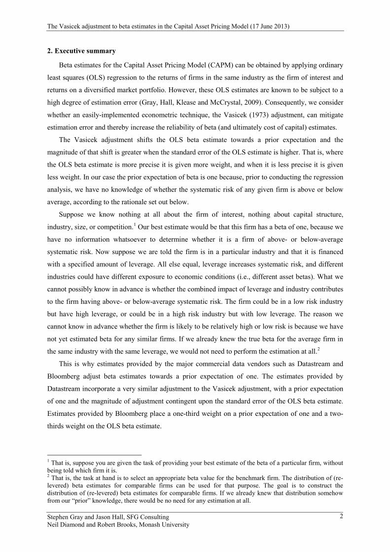
Turning to the regression results reported in Table 4, consider first the performance of expected

returns formed on the basis of OLS estimates. When we consider only observations in which at least

10 years of returns are available for beta estimation, expected returns are able to explain 56.59% of

the variation in realised portfolio returns. This is an improvement over the explanatory power of the

market itself, which is able to explain 54.54% of the variation in returns. The R-squared increases to

57.78% in the case of Vasicek-adjusted OLS estimates. So for the sample in which a long time series

of returns is available for analysis, Vasicek-adjusted estimates offer the greatest improvement in

explanatory power over the market return itself.

10 We cluster standard errors by portfolio because the same firm will often appear in the same portfolio over time, so the observations are not independent. 11 For example, the annualised return for stocks is computed as (1.0122)(365.25/28) – 1 = 0.171.



13

Table 3. Distribution of returns (%) Mean Std Dev Percentiles (%) 5th 25th 50th 75th 95th

Panel A: At least 131 periods used in beta estimation (N = 93,101) Stock return 1.22 20.06 –25.00 –7.98 0.00 7.15 33.31 Market return 0.73 4.40 –6.21 –1.57 1.21 3.38 6.51 Risk free rate 0.47 0.14 0.31 0.40 0.43 0.48 0.78 Excess stock return 0.74 20.06 –25.43 –8.43 –0.45 6.70 32.73 Excess market return 0.25 4.40 –6.62 –2.01 0.75 2.94 9.68 Panel B: At least 36 periods used in beta estimation (N = 247,652) Stock return 1.05 18.21 –23.18 –6.73 0.00 6.40 28.57 Market return 0.69 4.74 –6.36 –1.96 1.29 3.54 6.58 Risk free rate 0.48 0.17 0.31 0.40 0.43 0.47 0.97 Excess stock return 0.57 0.18 –23.62 –7.22 –0.42 5.91 28.12 Excess market return 0.21 4.73 –6.79 –2.59 0.76 3.08 6.09 In this table we summarise the distribution of stock returns, market returns and the risk free rate used in our test of whether expected returns are associated with market returns. Returns are computed over 343 four-week periods with the first period ending on 17 January 1986 and the last period ending on 4 May 2012. Summary statistics are computed using all firm-period observations. The sample considered in Panel A comprises 93,101 observations from 1,103 unique stocks in which at least 131 periods of returns (10 years equivalent) were available for beta estimation. The sample considered in Panel B comprises 247,652 observations from 2,585 unique stocks in which at least 36 periods of returns (2.75 years equivalent) were available for beta estimation.

For the larger sample in which at least 36 periods of returns are required for estimation, we

observe no incremental ability of expected returns derived from OLS estimates to explain portfolio

returns. If we impose the naïve assumption that all stocks have a beta estimate of one, we are able to

explain 49.55% of the variation in portfolio returns. The R-squared associated with OLS estimation is

47.88%. In contrast, expected returns derived from Vasicek-adjusted OLS estimates are able to

explain 51.88% of the variation in portfolio returns.

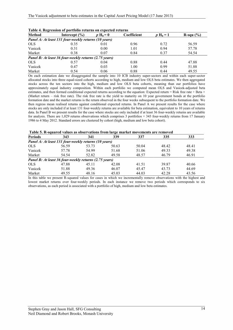
We examined whether our conclusions were sensitive to the inclusion or exclusion of a small

number of periods when market returns were unusually high or low. The 343 four-week periods

considered included one instance in which the market return was –34.4%, one instance in which the

market return was –22.3% and a further nine instances in which the market return was either below –

10% or above +10%. We repeated our analysis after excluding both the highest and lowest market

returns one at a time for up to 10 excluded periods, and observed the incremental change in

explanatory power. These results are presented in Table 5. In every instance we observe the same

relative explanatory power across the estimation techniques. Expected returns derived from Vasicek-

adjusted estimates have the highest explanatory power for both samples and for the larger sample, this

is the only measure of expected returns which has more explanatory power than the market itself.



14

Table 4. Regression of portfolio returns on expected returns Method Intercept (%) p H0 = 0 Coefficient p H0 = 1 R-squ (%) Panel A: At least 131 four-weekly returns (10 years) OLS 0.35 0.01 0.96 0.72 56.59 Vasicek 0.31 0.00 1.01 0.94 57.78 Market 0.38 0.07 0.84 0.37 54.54 Panel B: At least 36 four-weekly returns (2.75 years) OLS 0.57 0.04 0.88 0.44 47.88 Vasicek 0.47 0.03 1.00 0.99 51.88 Market 0.54 0.06 0.88 0.44 49.55 On each estimation date we disaggregated the sample into 10 ICB industry super-sectors and within each super-sector allocated stocks into three equal-sized cohorts according to high, medium and low OLS beta estimates. We then aggregated stocks across the ten sectors into the high, medium and low OLS beta cohorts, meaning than our portfolios have approximately equal industry composition. Within each portfolio we computed mean OLS and Vasicek-adjusted beta estimates, and then formed conditional expected returns according to the equation: Expected return = Risk free rate + Beta × (Market return – risk free rate). The risk free rate is the yield to maturity on 10 year government bonds at the portfolio formation date and the market returns is the return observed in the four weeks subsequent to the portfolio formation date. We then regress mean realised returns against conditional expected returns. In Panel A we present results for the case where stocks are only included if at least 131 four-weekly returns are available for beta estimation, equivalent to 10 years of returns data. In Panel B we present results for the case where stocks are only included if at least 36 four-weekly returns are available for analysis. There are 1,029 returns observations which comprises 3 portfolios × 343 four-weekly returns from 17 January 1986 to 4 May 2012. Standard errors are clustered by cohort (high, medium and low beta cohort).

Table 5. R-squared values as observations from large market movements are removed Periods 343 341 339 337 335 333 Panel A: At least 131 four-weekly returns (10 years) OLS 56.59 53.73 50.63 50.04 48.42 48.41 Vasicek 57.78 54.99 51.68 51.06 49.33 49.38 Market 54.54 52.82 49.58 48.57 46.79 46.91 Panel B: At least 36 four-weekly returns (2.75 years) OLS 47.88 45.11 42.08 41.51 39.87 40.66 Vasicek 51.88 49.36 46.07 45.47 43.73 44.69 Market 49.55 48.16 45.03 44.03 42.28 43.56 In this table we present R-squared values for cases in which we incrementally remove observations with the highest and lowest market returns over four-weekly periods. In each instance we remove two periods which corresponds to six observations, as each period is associated with a portfolio of high, medium and low beta estimates.



15

6. Conclusion

Four decades ago, researchers documented an important property of beta estimates from OLS

regression. Low beta estimates are likely to understate systematic risk and high beta estimates are

likely to overstate systematic risk. This was established both in statistical theory and empirical

practice. Estimates generated by Datastream and Bloomberg account for this tendency, by placing

some weight on the market average beta of one and some weight on the OLS beta estimate. The

Datastream adjustment is contingent upon the standard error of the beta estimate, while the

Bloomberg estimate places constant weight on a prior estimate of one.

The estimate we examine is the Vasicek-adjusted OLS estimate, which like the Datastream

estimate adjusts the OLS estimate towards one, with the magnitude of the adjustment contingent upon

the standard error. In the manner we have computed Vasicek-adjusted OLS estimates, it is easy to

implement and requires no subjective judgment. So for OLS estimates with a high standard error, it

offers a convenient technique for mitigating well-known statistical estimation error.

The primary argument against the use of the Vasicek adjustment is simply, “Why is the prior

expectation equal to one? Why isn’t the prior expectation something else, like the industry average?”

This argument can only be made if we know what the “something else” is, like the industry average.

But prior to measuring systematic risk we do not know whether the prior expectation of risk is higher

of lower than the average firm. If we have not yet measured systematic risk, how could we possibly

form a view that the combined impact of operating and financial risk leads to the firm’s beta being

above or below one?

Given there is support in theory, evidence and in practice for the Vasicek adjustment, the question

is whether it is useful. Does it generate beta estimates that are more reliable than OLS estimates? The

evidence suggests that it does. Vasicek-adjusted OLS estimates, when incorporated into the CAPM to

form expected returns, are able to predict stock returns to a limited degree. The Vasicek-adjusted OLS

estimates have more predictive ability than OLS estimates, but the improvement in explanatory power

is small. The implication is that cost of capital estimates formed using the Vasicek adjustment are

likely to be more reliable than estimates formed using unadjusted OLS estimates. There appears to be

no sound reason for not using this adjustment in estimating systematic risk.



16

7. References

Australian Energy Regulator, 2009. “Electricity transmission and distribution network service providers: Review of the weighted average cost of capital (WACC) parameters,” May 2009.

Blume, M.E., 1975. “Betas and their regression tendencies,” Journal of Finance, 30, 785–795. Cunningham, 1973. “Predictability of British Stock Market prices,” Journal of Royal Statistical

Society Series, 22, 315–331. Gray, S., J. Hall, D. Klease, and A. McCrystal, 2009. “Bias, stability and predictive ability in the

measurement of predictive risk,” Accounting Research Journal, 22, 220–236. Vasicek, O., 1973. “A note on using cross-sectional information in Bayesian estimation of security

betas,” Journal of Finance, 28, 1233–1239.



17

8. Appendix

To illustrate the statistical correction for estimation error via the application of Bayes’ Rule,

consider the following example.

Suppose the distribution of true betas is as follows:

True beta Probability 0.8 0.1 0.9 0.2 1.0 0.4 1.1 0.2 1.2 0.1

That is, true betas are distributed symmetrically around one. Also, suppose estimation error is

distributed as follows:

Estimation error Probability -0.1 1/3 0.0 1/3 0.1 1/3

That is, 40% of the stocks in the market have a true beta of 1.0. If you select one of those stocks

and find an estimate of its beta, there is a one third chance that the estimate will turn out to be 1.0, a

one third chance that the estimate will turn out to be 0.9 and a one third chance that the estimate will

turn out to be 1.1.



18

Now suppose that we want to find the best estimate of the true beta for a particular firm, given

that its beta estimate is 0.9. In this case, we know that there are three possible ways to obtain a beta

estimate of 0.9:

1. The true beta is 0.8 and estimation error is 0.1;

2. The true beta is 0.9 and estimation error is 0; or

3. The true beta is 1.0 and estimation error is -0.1.

Bayes’ Rule states that:

[ ] [ ] [ ][ ] 1429.0

233.01.033.0

9.0ˆPr8.0Pr8.0|9.0ˆPr9.0ˆ|8.0Pr =

×=

====

===β

βββββ

[ ] [ ] [ ][ ] 2857.0

233.02.033.0

9.0ˆPr9.0Pr9.0|9.0ˆPr9.0ˆ|9.0Pr =

×=

====

===β

βββββ

[ ] [ ] [ ][ ] 5714.0

233.04.033.0

9.0ˆPr0.1Pr0.1|9.0ˆPr9.0ˆ|0.1Pr =

×=

====

===β

βββββ

Consequently, the best estimate of the true beta, conditional on observing a beta estimate of 0.9 is:

[ ] 94.05714.00.12857.09.01429.08.09.0ˆ| =×+×+×==ββE

Bayes’ Rule can be applied to all beta estimates, giving the following forecasts conditional on

beta estimates:

Beta estimate Expected true beta 0.70 0.80 0.80 0.87 0.90 0.94 1.00 1.00 1.10 1.06 1.20 1.13 1.30 1.20

In summary, beta estimates must be adjusted towards one to eliminate statistical bias in

accordance with Bayes’ Rule. This is a well-known statistical correction for estimation error.

Note that this adjustment is required even though estimation error is symmetric. In the example

above, it is more likely that the true beta is 1.0 (with estimation error of -0.1) than 0.8 (with estimation

error of 0.1). This is because more stocks have a true beta of 1.0 than 0.8, and estimation error is

symmetric.

The Vasicek adjustment is simply an application of Bayes’ Rule to the case of continuous

probability distributions, rather than the simple discrete distributions used in this illustrative example.



19

9. Terms of reference and qualifications

This report was prepared by Professor Stephen Gray, Dr Jason Hall, Professor Robert Brooks and

Dr Neil Diamond. Professor Gray, Dr Hall, Professor Brooks and Dr Diamond have made all they

enquiries that they believe are desirable and appropriate and that no matters of significance that they

regard as relevant have, to their knowledge, been withheld.

Professor Gray, Dr Hall, Professor Brooks and Dr Diamond have been provided with a copy of

the Federal Court of Australia’s “Guidelines for Expert Witnesses in Proceeding in the Federal Court

of Australia.” The Report has been prepared in accordance with those Guidelines, which appear in the

terms of reference.

Documents

The Vasicek adjustment to beta estimates in the Capital ... · estimates in the Capital Asset Pricing Model . ... The Vasicek adjustment to beta estimates in the Capital Asset Pricing