The veriﬁcation Package - ftp.auckland.ac.nzftp.auckland.ac.nz/software/CRAN/doc/packages/verification.pdf · x A vector of forecast probabilities or a “prob.bin” class

The verification PackageJanuary 30, 2006

Version 1.09

Date January 30, 2006

Title Forecast verification utilities.

Author NCAR- Research Application Program

Maintainer Matt Pocernich <[email protected]>

Depends R (>= 2.1), fields, waveslim, boot, CircStats

Description This package contains utilities for verification of discrete,continuous, probabilisticforecasts and forecast expressed as parametric distributions.

License GPL Version 2 or later.

R topics documented:

analysis.dat . . . . . . . . . . . . . . . . . . . . . . . . . . . . . . . . . . . . . . . . .2attribute . . . . . . . . . . . . . . . . . . . . . . . . . . . . . . . . . . . . . . . . . . .2brier . . . . . . . . . . . . . . . . . . . . . . . . . . . . . . . . . . . . . . . . . . . . .3conditional.quantile . . . . . . . . . . . . . . . . . . . . . . . . . . . . . . . . . . . . .5crps . . . . . . . . . . . . . . . . . . . . . . . . . . . . . . . . . . . . . . . . . . . . .6crps.circ . . . . . . . . . . . . . . . . . . . . . . . . . . . . . . . . . . . . . . . . . . .7discrimination.plot . . . . . . . . . . . . . . . . . . . . . . . . . . . . . . . . . . . . .8forecast.dat . . . . . . . . . . . . . . . . . . . . . . . . . . . . . . . . . . . . . . . . .9int.scale.verify . . . . . . . . . . . . . . . . . . . . . . . . . . . . . . . . . . . . . . . .9leps . . . . . . . . . . . . . . . . . . . . . . . . . . . . . . . . . . . . . . . . . . . . .11lookup . . . . . . . . . . . . . . . . . . . . . . . . . . . . . . . . . . . . . . . . . . . .12measurement.error . . . . . . . . . . . . . . . . . . . . . . . . . . . . . . . . . . . . .12multi.cont . . . . . . . . . . . . . . . . . . . . . . . . . . . . . . . . . . . . . . . . . .13observation.error . . . . . . . . . . . . . . . . . . . . . . . . . . . . . . . . . . . . . .14plot.int.scale . . . . . . . . . . . . . . . . . . . . . . . . . . . . . . . . . . . . . . . . .15prob.frcs.dat . . . . . . . . . . . . . . . . . . . . . . . . . . . . . . . . . . . . . . . . .16probcont2disc . . . . . . . . . . . . . . . . . . . . . . . . . . . . . . . . . . . . . . . .17reliability.plot . . . . . . . . . . . . . . . . . . . . . . . . . . . . . . . . . . . . . . . .18roc.area . . . . . . . . . . . . . . . . . . . . . . . . . . . . . . . . . . . . . . . . . . .19roc.plot . . . . . . . . . . . . . . . . . . . . . . . . . . . . . . . . . . . . . . . . . . .20value . . . . . . . . . . . . . . . . . . . . . . . . . . . . . . . . . . . . . . . . . . . . .23verify-internal . . . . . . . . . . . . . . . . . . . . . . . . . . . . . . . . . . . . . . . .24verify . . . . . . . . . . . . . . . . . . . . . . . . . . . . . . . . . . . . . . . . . . . .25

1

2 attribute

Index 28

analysis.dat Spatial Observation Dataset.

Description

This spatial data set is used by theint.scale.verify function. This consists of the outcomeof the weather forecast presented inforecast.dat . This data was provided by Barabara Casatiand is from the Met Office.

attribute Attribute plot

Description

An attribute plot illustrates the reliability, resolution and uncertainty of a forecast with respect tothe observation. The frequency of binned forecast probabilities are plotted against proportions ofbinned observations. A perfect forecast would be indicated by a line plotted along the 1:1 line.Uncertainty is described as the vertical distance between this point and the 1:1 line. The relativefrequency for each forecast value is displayed in parenthesis.

Usage

## Default S3 method:attribute(x, obar.i, prob.y = NULL, obar = NULL, class ="none", main = NULL, CI = FALSE, n.boot = 100, alpha = 0.05, tck = 0.01, ...)## S3 method for class 'prob.bin':attribute(x, ...)

Arguments

x A vector of forecast probabilities or a “prob.bin” class object produced by theverify function.

obar.i A vector of observed relative frequency of forecast bins.

prob.y Relative frequency of forecasts of forecast bins.

obar Climatological or sample mean of observed events.

class Class of object. If prob.bin, the function will use the data to estimate confidenceintervals.

main Plot title.

CI Confidence Intervals. This is only an option if the data is accessible by using theverify command first. Calculated by bootstrapping the observations and predic-tion, then calculating PODy and PODn values.

n.boot Number of bootstrap samples.

alpha Confidence interval. By default = 0.05

tck Tick width on confidence interval whiskers.

... Graphical parameters

brier 3

Author(s)

Matt Pocernich <[email protected]>

References

Hsu, W. R., and A.H. Murphy, 1986: The attributes diagram: A geometrical framework for assess-ing the quality of probability forecasts.Int. J. Forecasting2, 285-293.

Wilks, D. S. (1995)Statistical Methods in the Atmospheric SciencesChapter 7, San Diego: Aca-demic Press.

See Also

verify

Examples

## Data from Wilks, table 7.3 page 246.y.i <- c(0,0.05, seq(0.1, 1, 0.1))obar.i <- c(0.006, 0.019, 0.059, 0.15, 0.277, 0.377, 0.511,

0.587, 0.723, 0.779, 0.934, 0.933)prob.y<- c(0.4112, 0.0671, 0.1833, 0.0986, 0.0616, 0.0366,

0.0303, 0.0275, 0.245, 0.022, 0.017, 0.203)obar<- 0.162

attribute(y.i, obar.i, prob.y, obar, titl = "Sample Attribute Plot")

## Function will work with a ``prob.bin'' class objects as well.## Note this is a random forecast.obs<- round(runif(100))pred<- runif(100)

A<- verify(obs, pred, frcst.type = "prob", obs.type = "binary")attribute(A, main = "Alternative plot", xlab = "Alternate x label" )## Same with confidence intervals

attribute(A, main = "Alternative plot", xlab = "Alternate x label", CI =TRUE)

brier Brier Score

Description

Calculates verification statistics for probabilistic forecasts of binary events.

Usage

brier(obs, pred, baseline, thresholds = seq(0,1,0.1), bins = TRUE, ... )

4 brier

Arguments

obs Vector of binary observations

pred Vector of probablistic predictions [0,1]

baseline Vector of climatological (no - skill) forecasts. If this is null, a sample climatol-ogy will be calculated.

thresholds Values used to bin the forecasts. By default the bins are {[0,0.1), [0.1, 0.2), ....}.

bins If TRUE, thresholds define bins into which the probablistic forecasts are enteredand assigned the midpoint as a forecast. Otherwise, each unique forecast isconsidered as a seperate forecast. For example, set bins to FALSE when dealingwith a finite number of probabilities generated by an ensemble forecast.

... Optional arguments

Value

baseline.tf Logical indicator of whether climatology was provided.

bs Brier score

bs.baseline Brier Score for climatology

ss Skill score

bs.reliabilityReliability portion of Brier score.

bs.resolutionResolution component of Brier score.

bs.uncert Uncertainty component of Brier score.

y.i Forecast bins – described as the center value of the bins.

obar.i Observation bins – described as the center value of the bins.

prob.y Proportion of time using each forecast

obar Forecast based on climatology or average sample observations.

check Reliability - resolution + uncertainty should equal brier score.

Note

This function is used withinverify .

Author(s)


References


conditional.quantile 5

Examples

# probabilistic/ binary example

pred<- runif(100)obs<- round(runif(100))

brier(obs, pred)

conditional.quantileConditional Quantile Plot

Description

This function creates a conditional quantile plot as shown in Murphy, et al (1989) and Wilks (1995).

Usage

conditional.quantile(pred, obs, bins = NULL, thrs = c(10, 20), main,... )

Arguments

pred Forecasted value.([n,1] vector, n = # of forecasts)

obs Observed value.([n,1] vector, n = # of observations)

bins Bins for forecast and observed values. A minimum number of values are re-quired to calculate meaningful statistics. So for variables that are continuous,such as temperature, it is frequently convenient to bin these values.([m,1] vec-tor, m = # of bins)

thrs The minimum number of values in a bin required to calculate the 25th and 75thquantiles and the 10th and 90th percentiles respectively. The median values willalways be displayed.( [2,1] vector)

main Plot title

... Plotting options.

Value

This function produces a conditional.quantile plot. They axis represents the observed values, whilethe x axis represents the forecasted values. The histogram along the bottom axis illustrates thefrequency of each forecast.

Note

In the example below, the median line extends beyond the range of the quartile or 10th and 90thpercentile lines. This is because there are not enough points in each bin to calculate these quartilevalues. That is, there are fewer than the limits set in thethrs input.

6 crps

Author(s)


References

Murphy, A. H., B.G. Brown and Y. Chen. (1989) “Diagnostic Verification of Temperature Fore-casts,”Weather and Forecasting; December, 1989.

Examples

set.seed(10)m<- seq(10, 25, length = 1000)frcst <- round(rnorm(1000, mean = m, sd = 2) )obs<- round(rnorm(1000, mean = m, sd = 2 ))bins <- seq(0, 30,1)thrs<- c( 10, 20) # number of obs needed for a statistic to be printed #1,4 quartile, 2,3 quartiles

conditional.quantile(frcst, obs, bins, thrs, main = "Sample Conditional Quantile Plot")#### Or plots a ``cont.cont'' class object.

obs<- rnorm(100)pred<- rnorm(100)baseline <- rnorm(100, sd = 0.5)

A<- verify(obs, pred, baseline = baseline, frcst.type = "cont", obs.type = "cont")plot(A)

crps Continuous Ranked Probability Score

Description

Calculates the crps for a forecast made in terms of a normal probability distribution and an obser-vation expressed in terms of a continuous variable.

Usage

crps(obs, pred, ...)

Arguments

obs A vector of observations.

pred A vector or matrix of the mean and standard deviation of a normal distribution.If the vector has a length of 2, it is assumed that these values represent themean and standard deviation of the normal distribution that will be used for allforecasts.


crps.circ 7

Value

crps Continous ranked probability scores

CRPS Mean of crps

ign Ignorance score

IGN Mean of the ignorance score

Note

This function is used withinverify .

Author(s)


References

Gneiting, T., Westveld, A., Raferty, A. and Goldman, T, 2004:Calibrated Probabilistic ForecastingUsing Ensemble Model Output Statistics and Minimum CRPS Estimation.Technical Report no.449, Department of Statistics, University of Washington. [ Available online athttp://www.stat.washington.edu/www/research/reports/ ]

Examples


x <- runif(100) ## simulated observation.crps(x, c(0,1))

## simulated forecast in which mean and sd differs for each forecast.frcs<- data.frame( runif(100, -2, 2), runif(100, 1, 3 ) )crps(x, frcs)

crps.circ CRPS Statistics for circular data

Description

Computes the circular CRPS when the verifying direction is ’x’ and the probabilistic forecast is avon Mises distribution on the circle with mean ’mu’ and concentration parameter ’kappa’.

Usage

crps.circ(x, mu, kappa )

Arguments

x A single direction in angles (0 <= x < 2 pi)

mu A single direction in angles (0 <= mu < 2 pi)

kappa A single positive number (kappa >= 0)

http://www.stat.washington.edu/www/research/reports/

http://www.stat.washington.edu/www/research/reports/

8 discrimination.plot

Value

crps.circ Circular crps

Author(s)

Nick Johnson<[email protected]>

References

Grimit, E.P., T. Gneiting, V.J. Berrocal and N.A. Johnson (2006). The continuous ranked probabilityscore for circular variables and its application to mesoscale forecast ensemble verification. ,132,pp. 1-17,Q.J.R. Meteorolo. Soc..

Examples

x <- pi/3mu <- pi/3.2kappa <- 10000ES.VM.Comp2.Max.Kappa <- 1500

crps.circ( x = pi/3, mu = pi/3.2, kappa = 10000)

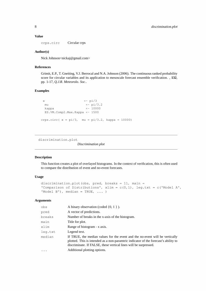
discrimination.plotDiscrimination plot

Description

This function creates a plot of overlayed histograms. In the context of verification, this is often usedto compare the distribution of event and no-event forecasts.

Usage

discrimination.plot(obs, pred, breaks = 11, main ="Comparison of Distributions", xlim = c(0,1), leg.txt = c("Model A","Model B"), median = TRUE, ... )

Arguments

obs A binary observation (coded {0, 1 } ).

pred A vector of predictions.

breaks Number of breaks in the x-axis of the histogram.

main Title for plot.

xlim Range of histogram - x axis.

leg.txt Legend text.

median If TRUE, the median values for the event and the no-event will be verticallyplotted. This is intended as a non-paramtric indicator of the forecast’s ability todiscriminate. If FALSE, these vertical lines will be surpressed.

... Additional plotting options.

forecast.dat 9

Author(s)


Examples

# A sample forecast.

a<- rnorm(100, mean = -1); b<- rnorm(100, mean = 1)

A<- cbind(rep(0,100), pnorm(a)); B<- cbind(rep(1,100), pnorm(b))

dat<- rbind(A,B); dat<- as.data.frame(dat)names(dat)<- c("obs", "pred")

discrimination.plot(dat$obs, dat$pred, main = "Sample Plot")

forecast.dat Forecast forecast dataset.

Description

This spatial data set is an example used by theint.scale.verify function. It consists of theNimrod forecasting system and was provided by Barbara Casati.

int.scale.verify Intensity-Scale Verification Model

Description

For a spatial forecast, evaluates the forecast skill as a function of precipitaion rate intesity and spatialscale of the error.

Usage

int.scale.verify(frcs, obs, thres = quantile(frcs, p = seq(0,0.9,0.1)), ... )

Arguments

frcs Forecast matrix. Must be of2n dimensions.

obs Observation matrix. Must be of2n dimensions.

thres A vector of thresholds to be considered. By default, the percentiles 0, 90 areused.

... Optional arguments may be passed to the image plot

10 int.scale.verify

Value

SSul Skill score as matrix. The rownames are the thresholds, the colnames arenwhere2n is the spatial scale of the skill score decomposition.

MSE A matrix with the mean squared error of the forecast

l.frcs Number of rows in forecast. Used in plotting routine.

thres Thresholds used in model

Note

This function creates an image plot of the intensity plot of the skill scores as a function of spatialscale and threshold. The top row is equivalent to the bias of the forecast.

Author(s)

Barabara Casati <barbara.casati (at) ec.gc.ca>

References

B.Casati, D.B. Stephenson, G. Ross.A new intensity-scale approach for the verification of spatialprecipitation forecasts. Meteorological Application (RMS), in press.

See Also

http://www.met.rdg.ac.uk/~swr00bc/

Examples

## simulated examplen<- 5set.seed(10)forecast1 <- matrix( log(rlnorm(n = (2^n *2^n) )) , nrow = 2^n)obs1 <- matrix(log( rlnorm(n = (2^n *2^n) )) , nrow = 2^n)int.scale.verify(forecast1, obs1, main = "Test Case")

## real example. Data source referenced below.

data(analysis.dat)data(forecast.dat)

require(waveslim)require(fields)

A<- int.scale.verify(forecast.dat, analysis.dat,thres = c(0, 2^seq(-5,6)), main = "NIMROD example" )

plot(A)

http://www.met.rdg.ac.uk/~swr00bc/

leps 11

leps Linear Error in Probability Space (LEPS)

Description

Calculates the linear error in probability spaces. This is the mean absolute difference between theforecast cumulative distribution value (cdf) and the observation. This function creates the empiricalcdf function for the observations using the sample population. Linear interpretation is used toestimate the cdf values between observation values. Therefore; this may produce awkward resultswith small datasets.

Usage

leps(x, pred, plot = TRUE, ... )

Arguments

x A vector of observations or a verification object with “cont.cont” properties.

pred A vector of predictions.

plot Logical to generate a plot or not.


Value

If assigned to an object, the following values are reported.

leps.0 Negatively oriented score on the [0,1] scale, where 0 is a perfect score.

leps.1 Positively oriented score proposed by Potts.

Author(s)


References

DeQue, Michel. (2003) “Continuous Variables”Chapter 5, Forecast Verification: A Practitioner’sGuide in Atmospheric Science.

Potts, J. M., Folland, C.K., Jolliffe, I.T. and Secton, D. (1996) “Revised ‘LEPS’ scores fore assess-ing climate model simulations and long-range forecasts.”J. Climate, 9, pp. 34-54.

Examples

obs <- rnorm(100, mean = 1, sd = sqrt(50))pred<- rnorm(100, mean = 10, sd = sqrt(500))

leps(obs, pred, main = "Sample Plot")## values approximated

OBS <- c(2.7, 2.9, 3.2, 3.3, 3.4, 3.4, 3.5, 3.8, 4, 4.2, 4.4, 4.4, 4.6,5.8, 6.4)

12 measurement.error

PRED <- c(2.05, 3.6, 3.05, 4.5, 3.5, 3.0, 3.9, 3.2, 2.4, 5.3, 2.5, 2.8,3.2, 2.8, 7.5)

a <- leps(OBS, PRED)a

lookup Lookup table for crps.circ.

Description

Saved lookup data to expedite integration in the crps.circ function.

See Also

crps.circ

measurement.error Skill score with measurement error.

Description

Skill score that incorporates measurement error. This function allows the user to incorporate mea-surement error in an observation in a skill score.

Usage

measurement.error( obs, frcs = NULL, theta = 0.5, CI =FALSE, t = 1, u = 0, h = NULL, ...)

Arguments

obs Information about a forecast and observation can be done in one of two ways.First, the results of a contingency table can be entered as a vector containingc(n11, n10, n01, n00), where n11 are the number of correctly predicted eventsand n01 is the number of incorrectly predicted non-events. Actual forecasts andobservations can be used. In this case, obs is a vector of binary outcomes [0,1].

frcs If obs is entered as a contingency table, this agrument is null. If obs is a vectorof outcomes, this column is a vector of probablistic forecasts.

theta Loss value (cost) of making a incorrect forecast by a non-event. Defaults to 0.5.

CI Calculate confidence intervals for skill score.

t Probability of forecasting an event, when an event occurs. A perfect value is 1.

u Probability of forecasting that no event will occur, when and event occurs. Aperfect value is 0.

h Threshold for converting a probablistic forecast into a binary forecast. By de-fault, this value is NULL and the theta is used as this threshold.

... Optional arguments.

multi.cont 13

Value

z Error code

k Skill score

G Likelihood ratio statistic

p p-value for the null hypothesis that the forecast contains skill.

theta Loss value. Loss associated with an incorrect forecast of a non-event.

ciLO Lower confidence interval

ciHI Upper confidence interval

Author(s)

Matt Pocernich <[email protected]> (R - code)

W.M Briggs <wib2004(at)med.cornell.edu> (Method questions)

References

W.M. Briggs, 2004.Incorporating Cost in the Skill ScoreTechnical Report, wm-briggs.com/public/skillocst.pdf.

W.M. Briggs and D. Ruppert, 2004.Assessing the skill of yes/no forecasts. Submitting to Biomet-rics.

J.P. Finley, 1884. Tornado forecasts.Amer. Meteor. J.85-88. (Tornado data used in example.)

Examples

DAT<- data.frame( obs = round(runif(50)), frcs = runif(50))

A<- measurement.error(DAT$obs, DAT$frcs, CI = TRUE)A### Finley Data

measurement.error(c(28, 23, 72, 2680)) ## assuming perfect observation,

multi.cont Multiple Contingency Table Statistics

Description

Provides a variety of statistics for a data summarized in a contingency table. This will work for a 2by 2 table, but is more useful for tables of greater dimensions.

Usage

multi.cont(DAT)

Arguments

DAT A contingency table in the form of a matrix. It is assumed that columns representobservation, rows represent forecasts.

14 observation.error

Value

pc Percent correct - events along the diagonal.

bias Bias

pod Probability of detecting an event.

far False Alarm Rate

ts Threat score a.k.a. Critical success index (CSI)

hss Heidke Skill Score

pss Pierce Skill Score

gs Gerrity Score

Author(s)


References

Gerrity, J.P. Jr (1992). A note on Gandin and Murphy’s equitable skill score.Mon. Weather Rev.,120, 2707-2712.

Jolliffe, I.T. and D.B. Stephenson (2003). Forecast verification: a practitioner’s guide in atmo-spheric science. John Wiley and Sons. See chapter 4 concerning categorical events, written by R.E. Livezey.

Examples

DAT<- matrix(c(7,4,4,14,9,8,14,16,24), nrow = 3) # from p. 80 - Jolliffemulti.cont(DAT)

DAT<- matrix(c(3,8,7,8,13,14,4,18,25), ncol = 3) ## Jolliffe JJAmulti.cont(DAT)

DAT<- matrix(c(50,47,54,91,2364,205,71,170,3288), ncol = 3) # Wilks p. 245multi.cont(DAT)

DAT<- matrix(c(28, 23, 72, 2680 ), ncol = 2) ## Finleymulti.cont(DAT)

observation.error Observation Error

Description

Quantifies observation error through use of a “Gold Standard” of observations.

Usage

observation.error(obs, gold.standard = NULL, ...)

plot.int.scale 15

Arguments

obs Observation made by method to be quantified. This information can be enteredtwo ways. If obs is a vector of length 4, it is assumed that is contains the valuesc(n11, n10, n01, n00), where n11 are the number of correctly predicted eventsand n01 is the number of incorrectly predicted non-events.

gold.standardThe gold standard. This is considered a higher quality observation (coded {0, 1} ).

... Optional arguments.

Value

t Probability of forecasting an event, when an event occurs. A perfect value is 1.

u Probability of forecasting that no event will occur, when and event occurs. Aperfect value is 0.

Note

This function is used to calculate values for themeasurement.error function.

Author(s)


See Also

measurement.error

Examples

obs <- round(runif(100))gold <- round(runif(100) )observation.error(obs, gold)

## Pirep gold standard

observation.error(c(43,10,17,4) )

plot.int.scale Plot Intensity Scale Objects.

Description

Plots objects from theint.scale.verify using theimage function from the base packageandimage.plot from the fields package..

Usage

plot.int.scale(x, y = NULL, plot.mse = FALSE, main = NULL, ...)

16 prob.frcs.dat

Arguments

x A object from theint.scale.verify function that has the class int.scale.

y NULL

plot.mse Should a plot be created of the mean squared errors? By default the skill scoresare plotted.

main Plot title


Author(s)


See Also

int.scale.verify , image , image.plot

Examples

data(analysis.dat)data(forecast.dat)

A<- int.scale.verify(forecast.dat, analysis.dat, thres = c(0, 2^seq(-5,6)))plot(A)plot(A, plot.mse = TRUE)plot(A, main = "Test case")

prob.frcs.dat Probablisitic Forecast Dataset.

Description

This data set is used as an example of data used by theroc.plot function. The first columncontains a probablisitic forecast for aviation icing. The second column contains a logical variableindicating whether or not icing was observed.

References

PROBABILITY FORECASTS OF IN-FLIGHT ICING CONDITIONSBarbara G. Brown, Ben C.Bernstein, Frank McDonough and Tiffany A. O. Bernstein, 8th Conference on Aviation, Range,and Aerospace Meteorology, Dallas TX, 10-15 January 1999.

probcont2disc 17

probcont2disc Converts continuous probability values into binned discrete probabil-ity forecasts.

Description

Converts continuous probability values into binned discrete probability forecasts. This is useful incalculated Brier type scores for values with continuous probabilities. Each probability is assignedthe value of the midpoint.

Usage

probcont2disc(x, bins = seq(0,1,0.1) )

Arguments

x A vector of probabilities

bins Bins. Defaults to 0 to 1 by 0.1 .

Value

A vector of discrete probabilities. E

Note

This function is used withinbrier .

Author(s)


Examples


set.seed(1)x <- runif(10) ## simulated probabilities.

probcont2disc(x)probcont2disc(x, bins = seq(0,1,0.25) )

## probcont2disc(4, bins = seq(0,1,0.3)) ## gets error

18 reliability.plot

reliability.plot Reliability Plot

Description

A reliability plot is a simple form of an attribute diagram that depicts the performance of a prob-abilistic forecast for a binary event. In this diagram, the forecast probability is plotted against theobserved relative frequency. Ideally, this value should be near to each other and so points falling onthe 1:1 line are desirable. For added information, if one or two forecasts are being verified, sharp-ness diagrams are presented in the corners of the plot. Ideally, these histograms should be relativelyflat, indicating that each bin of probabilities is use an appropriate amount of times.

Usage

## Default S3 method:reliability.plot(x, obar.i, prob.y, titl = NULL, legend.names = NULL, ... )

## S3 method for class 'verify':reliability.plot(x, ...)

Arguments

x Forecast probabilities.(yi) or a “prob.bin” class object fromverify .

obar.i Observed relative frequencyoi.

prob.y Relative frequency of forecasts

titl Title

legend.names Names of each model that will appear in the legend.

... Graphical parameters.

Details

This function works either by entering vectors or on a verify class object.

Note

If a single prob.bin class object is used, a reliability plot along with a sharpness diagram is displayed.If two forecasts are provided in the form of a matrix of predictions, two sharpness diagrams areprovided. If more forecasts are provided, the sharpness diagrams are not displayed.

Author(s)


References


roc.area 19

Examples

## Data from Wilks, table 7.3 page 246.y.i <- c(0,0.05, seq(0.1, 1, 0.1))obar.i <- c(0.006, 0.019, 0.059, 0.15, 0.277, 0.377, 0.511, 0.587, 0.723, 0.779, 0.934, 0.933)prob.y<- c(0.4112, 0.0671, 0.1833, 0.0986, 0.0616, 0.0366, 0.0303, 0.0275, 0.245, 0.022, 0.017, 0.203)obar<- 0.162

reliability.plot(y.i, obar.i, prob.y, titl = "Test 1", legend.names =c("Model A") )

## Function will work with a ``prob.bin'' class object as well.## Note this is a very bad forecast.obs<- round(runif(100))pred<- runif(100)

A<- verify(obs, pred, frcst.type = "prob", obs.type = "binary")

reliability.plot(A, titl = "Alternative plot")

roc.area Area under curve (AUC) calculation for Response Operating Charac-teristic curve.

Description

This function calculates the area underneath a ROC curve following the process outlined in Ma-son and Graham (2002). The p-value produced is related to the Mann-Whitney U statistics. Thep-value is calculated using the wilcox.test function which automatically handles ties and makesapproximations for large values.

The p-value addresses the null hypothesisHo : The area under the ROC curve is 0.5 i.e. the forecasthas no skill.

Usage

roc.area(obs, pred)

Arguments

obs A binary observation (coded {0, 1 } ).

pred A probability prediction on the interval [0,1].

Value

A Area under ROC curve, adjusted for ties in forecasts, if present

n.total Total number of records

n.events Number of events

n.noevents Number of non-events

p.value Unadjusted p-value

20 roc.plot

Note

This function is used internally in theroc.plot command to calculate areas.

Author(s)


References

Mason, S.J. and N.E. Graham. (2002) “Areas beneath the relative operating characteristics (ROC)and relative operating levels (ROL) curves: Statistical significance and interpretation, ”Q. J. R.Meteorol. Soc.30 (1982) 291-303.

See Also

roc.plot , verify , wilcox.test

Examples

# Data used from Mason and Graham (2002).a<- c(1981, 1982, 1983, 1984, 1985, 1986, 1987, 1988, 1989, 1990,

1991, 1992, 1993, 1994, 1995)b<- c(0,0,0,1,1,1,0,1,1,0,0,0,0,1,1)c<- c(.8, .8, 0, 1,1,.6, .4, .8, 0, 0, .2, 0, 0, 1,1)d<- c(.928,.576, .008, .944, .832, .816, .136, .584, .032, .016, .28, .024, 0, .984, .952)

A<- data.frame(a,b,c, d)names(A)<- c("year", "event", "p1", "p2")

## for model with tiesroc.area(A$event, A$p1)

## for model without tiesroc.area(A$event, A$p2)

roc.plot Relative operating characteristic curve.

Description

This function creates Receiver Operating Characteristic (ROC) plots for one or more models. AROC curve plots the false alarm rate against the hit rate for a probablistic forecast for a range ofthresholds. The area under the curve is viewed as a measure of a forecast’s accuracy. A measure of1 would indicate a perfect model. A measure of 0.5 would indicate a random forecast.

Usage

## Default S3 method:roc.plot(x, pred, thresholds = NULL, binormal =

FALSE, legend = FALSE, leg.text = NULL, plot = "emp", CI = FALSE,n.boot = 1000, alpha = 0.05, tck = 0.01, plot.thres = seq(0.1,0.9, 0.1), show.thres = TRUE, main = "ROC Curve", xlab = "False Alarm Rate", ylab = "Hit Rate", extra = FALSE, ...)

roc.plot 21

## S3 method for class 'prob.bin':roc.plot(x, ...)

Arguments

x A binary observation (coded {0, 1 } ) or a verification object.

pred A probability prediction on the interval [0,1]. If multiple models are compared,this may be a matrix where each column represents a different prediction.

thresholds Thresholds may be provided. These thresholds will be used to calculate the hitrate (h) and false alarm rate (f ). If thresholds is NULL, all unique thresholds areused as a threshold. Alternatively, if the number of bins is specified, thresholdswill be calculated using the specified numbers of quantiles.

binormal If TRUE, in addition to the empirical ROC curve, the binormal ROC curve willbe calculated. To get a plot draw, plot must be either “binorm” or “both”.

legend Binomial. Defaults to FALSE indicating whether a legend should be displayed.

leg.text Character vector for legend. If NULL, models are labeled “Model A", “ModelB",...

plot Either “emp” (default), “binorm” or “both” to determine which plot is shown. Ifset to NULL, a plot is not created

CI Confidence Intervals. Calculated by bootstrapping the observations and predic-tion, then calculating PODy and PODn values.

n.boot Number of bootstrap samples.

alpha Confidence interval. By default = 0.05

tck Tick width on confidence interval whiskers.

plot.thres By default, displays the threshold levels on the ROC diagrams. To surpress thesevalues, set it equal to NULL. If confidence intervals (CI) is set to TRUE, levelsspecified here will determine where confidence interval boxes are placed.

show.thres Show thresholds for points indicated by plot.thres. Defaults to TRUE.

main Title for plot.

xlab, ylab Plot axes labels. Defaults to “Hit Rate” and “False Alarm Rate”, for the y and xaxes respectively.

extra Extra text describing binormal and empirical lines.


Value


plot.data The data used to generate the ROC plots. This is a array. Column headers arethresholds, empirical hit and false alarm rates, and binormal hit and false alarmrates. Each model is depicted on an array indexed by the third dimension.

roc.vol The areas under the ROC curves. By default,this is printed on the plots. Areasand p-values are calculated with and without adjustments for ties along with thep-value for the area. These values are calculated usingroc.area . The fifthcolumn contains the area under the binormal curve, if binormal is selected.

Note

There is not a minimum size required to create confidence limits or show thresholds. When thereare few data points, it is possilbe to make some pretty unattractive graphs.

22 roc.plot

Author(s)


References

Mason, I. (1982) “A model for assessment of weather forecasts,”Aust. Met. Mag30 (1982) 291-303.

Mason, S.J. and N.E. Graham. (2002) “Areas beneath the relative operating characteristics (ROC)and relative operating levels (ROL) curves: Statistical significance and interpretation, ”Q. J. R.Meteorol. Soc.128pp. 2145-2166.

Swets, John A. (1996)Signal Detection Theory and ROC Analysis in Psychology and Diagnostics,Lawrence Erlbaum Associates, Inc.

Examples

# Data from Mason and Graham article.

a<- c(0,0,0,1,1,1,0,1,1,0,0,0,0,1,1)b<- c(.8, .8, 0, 1,1,.6, .4, .8, 0, 0, .2, 0, 0, 1,1)c<- c(.928,.576, .008, .944, .832, .816, .136, .584, .032, .016, .28, .024, 0, .984, .952)

A<- data.frame(a,b,c)names(A)<- c("event", "p1", "p2")

## for model with tiesroc.plot(A$event, A$p1)

## for model without tiesroc.plot(A$event, A$p2)

### show binormal curve fit.

roc.plot(A$event, A$p2, binormal = TRUE)

# icing forecast

data(prob.frcs.dat)A <- verify(prob.frcs.dat$obs, prob.frcs.dat$frcst/100)roc.plot(A, main = "AWG Forecast")

# plotting a ``prob.bin'' class object.obs<- round(runif(100))pred<- runif(100)

A<- verify(obs, pred, frcst.type = "prob", obs.type = "binary")

roc.plot(A, main = "Test 1", binormal = TRUE, plot = "both")

## show confidence intervals. MAY BE SLOWroc.plot(A, threshold = seq(0.1,0.9, 0.1), main = "Test 1", CI = TRUE,alpha = 0.1)

value 23

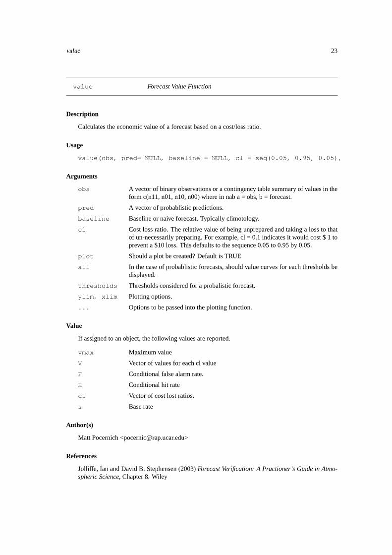
value Forecast Value Function

Description

Calculates the economic value of a forecast based on a cost/loss ratio.

Usage

value(obs, pred= NULL, baseline = NULL, cl = seq(0.05, 0.95, 0.05), plot = TRUE, all = FALSE, thresholds = seq(0.05, 0.95, 0.05), ylim = c(-0.1, 0.5), xlim = c(0,1), ...)

Arguments

obs A vector of binary observations or a contingency table summary of values in theform c(n11, n01, n10, n00) where in nab a = obs, b = forecast.

pred A vector of probablistic predictions.

baseline Baseline or naive forecast. Typically climotology.

cl Cost loss ratio. The relative value of being unprepared and taking a loss to thatof un-necessarily preparing. For example, cl = 0.1 indicates it would cost $ 1 toprevent a $10 loss. This defaults to the sequence 0.05 to 0.95 by 0.05.

plot Should a plot be created? Default is TRUE

all In the case of probablistic forecasts, should value curves for each thresholds bedisplayed.

thresholds Thresholds considered for a probalistic forecast.

ylim, xlim Plotting options.

... Options to be passed into the plotting function.

Value


vmax Maximum value

V Vector of values for each cl value

F Conditional false alarm rate.

H Conditional hit rate

cl Vector of cost lost ratios.

s Base rate

Author(s)


References

Jolliffe, Ian and David B. Stephensen (2003)Forecast Verification: A Practioner’s Guide in Atmo-spheric Science, Chapter 8. Wiley

24 verify-internal

Examples

## value as a contigency table## Finley tornado data

obs<- c(28, 72, 23, 2680)value(obs)aa <- value(obs)aa$Vmax # max value

## probablistic forecast exampleobs <- round(runif(100) )pred <- runif(100)

value(obs, pred, main = "Sample Plot",thresholds = seq(0.02, 0.98, 0.02) )

verify-internal Verification internal and secondary functions

Description

Listed below are either internal functions or secondary functions.

Usage

table.stats(obs, pred = NULL)summary.prob.bin(object, ...)summary.bin.bin(object, ...)summary.cont.cont(object, ...)summary.norm.dist.cont(object, ...)summary.cat.cat(object, ...)ranked.hist(frcst, nbins = 10, titl = NULL)plot.prob.bin(x, ...)plot.cont.cont(x, ...)roc(x, pred, thres, binormal, ...)zzz

angle.dist(a, b)calc.ES.VM.comp1(kappa, mc.size)ES.VM.comp1(kappa)ES.VM.comp1.array(kappa)

approx.comp2(x, mu, kappa)dvm2(theta, mu, kappa)ES.VM.comp2(x, mu, k)ES.VM.comp2.array(x, mu, k)

verify 25

verify Verification function

Description

Based on the type of inputs, this function calculates a range of verification statistics and skill scores.Additionally, it creates a verify class object that can be further analyzed.

Usage

verify(obs, pred, baseline = NULL,frcst.type = "prob", obs.type = "binary", thresholds =

seq(0,1,0.1), show = TRUE )

Arguments

obs The values with which the verifications are verified. May be a vector of length4 if the forecast and predictions are binary data summarized in a contingencytable. In this case, the value are entered in the order of c(n11, n01, n10, n00).

pred Prediction of event. The prediction may be in the form of the a point predictionor the probability of a forecast. Let pred = NULL if obs represents a contingencytable.

baseline In meteorology, climatology is the baseline that represents the no-skill forecast.In other fields this field would differ. This field is used to calculate certain skillscores. If left NULL, these statistics are calculated using sample climatology.

frcst.type Forecast type. Either "prob", "binary", "norm.dist", "cat" or "cont". Defaultsto "prob". "norm.dist" is used when the forecast is in the form of a normaldistribution. See crps for more details.

obs.type Observation type. Either "binary", "cat" or "cont". Defaults to "binary"

thresholds Thresholds to be considered for point forecasts of continuous events.

show Logical; if TRUE (the default), print warning message

Value

An object of the verify class. Depending on the type of data used, the following information may bereturned. The following notation is used to describe which values are produced for which type offorecast/observations. (BB = binary/binary, PB = probablistic/binary, CC = continuous/continuous,CTCT = categorical/categorical)

BS Brier Score (PB)

BSS Brier Skill Score(PB)

SS Skill Score (BB)

hit.rate Hit rate, aka PODy,h (PB, CTCT)false.alarm.rate

False alarm rate, PODn,f (PB, CTCT)

TS Threat Score or Critical Success Index (CSI)(BB, CTCT)

ETS Equitable Threat Score (BB, CTCT)

26 verify

BIAS Bias (BB, CTCT)

PC Percent correct or hit rate (BB, CTCT)

Cont.Table Contingency Table (BB)

HSS Heidke Skill Score(BB, CTCT)

KSS Kuniper Skill Score (BB)

PSS Pierce Skill Score (CTCT)

GS Gerrity Score (CTCT)

ME Mean error (CC)

MSE Mean-squared error (CC)

MAE Mean absolute error (CC)

Note

For the categorical forecast and verification, the Gerrity score only makes sense for forecast thathave order, or are basically ordinal. It is assumed that the forecasts are listed in order. For example,low, medium and high would get translated into 1,2 and 3.

Author(s)


References


WMO Joint WWRP/WGNE Working Group on Verification Website

http://www.bom.gov.au/bmrc/wefor/staff/eee/verif/verif_web_page.html

Examples

# binary/binary exampleobs<- round(runif(100))pred<- round(runif(100))

# binary/binary Finley tornado data.

obs<- c(28, 72, 23, 2680)A<- verify(obs, pred = NULL, frcst.type = "binary", obs.type = "binary")

summary(A)

# categorical/categorical example

obs <- round(runif(100, 1,5) )pred <- round(runif(100, 1,5) )

A<- verify(obs, pred, frcst.type = "cat", obs.type = "cat" )summary(A)

# probabilistic/ binary examplepred<- runif(100)A<- verify(obs, pred, frcst.type = "prob", obs.type = "binary")

http://www.bom.gov.au/bmrc/wefor/staff/eee/verif/verif_web_page.html

verify 27

summary(A)# continuous/ continuous exampleobs<- rnorm(100)pred<- rnorm(100)baseline <- rnorm(100, sd = 0.5)

A<- verify(obs, pred, baseline = baseline, frcst.type = "cont", obs.type = "cont")summary(A)

Index

∗Topic datasetsanalysis.dat , 1forecast.dat , 9lookup , 12prob.frcs.dat , 16

∗Topic fileattribute , 2brier , 3conditional.quantile , 5crps , 6crps.circ , 7discrimination.plot , 8int.scale.verify , 9leps , 10measurement.error , 12multi.cont , 13observation.error , 14plot.int.scale , 15probcont2disc , 17reliability.plot , 18roc.area , 19roc.plot , 20value , 23verify , 25

∗Topic internalverify-internal , 24

analysis.dat , 1angle.dist (verify-internal ), 24approx.comp2 (verify-internal ), 24attribute , 2attribute.prob.bin (attribute ), 2

brier , 3

calc.ES.VM.comp1(verify-internal ), 24

conditional.quantile , 5crps , 6crps.circ , 7, 12

discrimination.plot , 8dvm2 (verify-internal ), 24

ES.VM.comp1 (verify-internal ), 24

ES.VM.comp2 (verify-internal ), 24

forecast.dat , 1, 9

image , 16image.plot , 16int.scale.verify , 1, 9, 9, 15, 16

leps , 10lookup , 12

measurement.error , 12, 15multi.cont , 13

observation.error , 14

plot.cont.cont (verify-internal ),24

plot.int.scale , 15plot.prob.bin (verify-internal ),

24prob.frcs.dat , 16probcont2disc , 17

ranked.hist (verify-internal ), 24reliability.plot , 18roc (verify-internal ), 24roc.area , 19, 21roc.plot , 20, 20roc.plot.prob.bin (roc.plot ), 20

summary.bin.bin(verify-internal ), 24

summary.cat.cat(verify-internal ), 24

summary.cont.cont(verify-internal ), 24

summary.norm.dist.cont(verify-internal ), 24

summary.prob.bin(verify-internal ), 24

table.stats (verify-internal ), 24

value , 23

28

INDEX 29

verify , 3, 20, 25verify-internal , 24

wilcox.test , 20

zzz (verify-internal ), 24

Documents

The veriﬁcation Package - ftp.auckland.ac.nzftp.auckland.ac.nz/software/CRAN/doc/packages/verification.pdf · x A vector of forecast probabilities or a “prob.bin” class