The Violent Legacy of Victimization: Post-Conflict Evidence on

Asylum Seekers, Crimes and Public Policy in Switzerland ∗

Mathieu Couttenier† Veronica Preotu‡ Dominic Rohner§ Mathias Thoenig¶

September 6, 2016

Abstract

We study empirically how past exposure to conflict in origin countries makes migrants moreviolent prone in their host country, focusing on asylum seekers in Switzerland. We exploit anovel and unique dataset on all crimes reported in Switzerland by nationalities of perpetratorsand victims over the period 2009-2012. Causal analysis relies on the fact that asylum seekersare exogenously allocated across the Swiss territory by the federal administration. Our baselineresult is that cohorts exposed to civil conflicts/mass killings during childhood are on average 40percent more prone to violent crimes than their co-nationals born after the conflict. The effectis stable through the lifecycle and is attenuated for women, for property crimes and for low-intensity conflicts. Further, a bilateral crime regression shows that conflict exposed cohorts havea higher propensity to target victims from their own nationality –a piece of evidence that weinterpret as persistence in intra-national grievances. Last, we exploit cross-region heterogeneityin public policies within Switzerland to document which integration policies are able to mitigatethe detrimental effect of past conflict exposure on violent criminality. In particular, we find thatoffering labor market access to asylum seekers and fostering social integration eliminates all theeffect.

Keywords: Violent Crime, Persistence of Violence, Civil Conflict, Mass Killing, Migration,Refugees.

JEL Classification: D74, F22, K42, Z18.

∗We thank Markus Hersche, Laurenz Baertsch and Timothy Schaffer for excellent research assistance. Helpfulcomments from Yann Algan, Nicolas Berman, Marius Bruhlhart, Matteo Cervellati, Paola Conconi, Quoc-Anh Do,Denise Efionayi-Mader, John Huber, Erzo Luttmer, Thierry Mayer, Maria Petrova, Nicolas van de Sijpe, Uwe Sunde,Jean-Claude Thoenig, and Katia Zhuravskaya, as well as participants to seminars and conferences at NBER SI politicaleconomy group, 4th TEMPO CEPR conference in Nottingham, Warwck/Princeton Political Economy Conferencein Venice, Political Economy Workshop at NYU, Barcelona GSE Summer Forum, EEA Annual meeting in Geneva,Bologna, Lausanne, Paris School of Economics, Autonoma Barcelona, Lucerne, Cergy, Montpellier, Graduate InstituteGeneva, Lille, Paris 1, Oxford, Bath, Sheffield and Paris Dauphine are gratefully acknowledged. Mathieu Couttenierand Mathias Thoenig acknowledge financial support from the ERC Starting Grant GRIEVANCES-313327, andDominic Rohner gratefully acknowledged funding from the SNF-grant ”The Economics of Ethnic Conflict” (100017-150159 / 1). We kindly thank as well Anne-Corinne Vollenweider and Philippe Hayoz from Swiss Federal StatisticsOffice and Beat Friedli, Veronika Moser, Pierre-Yves Dubois and Simon Sieber of the Swiss Federal Office for Migrationfor sharing their exhaustive data on crime and asylum seekers with us, and Nicole Wichmann and various cantonalauthorities for providing information on cantonal integration policies.†University of Geneva, mathieu.couttenier@unige.ch‡University of Geneva, veronica.preotu@unige.ch§University of Lausanne and CEPR, dominic.rohner@unil.ch¶University of Lausanne and CEPR, mathias.thoenig@unil.ch

1 Introduction

Violence breeds violence. Political violence is often persistent and wars tend to recur,1 and there

is much anecdotal evidence that exposure to a conflict context makes people more violence prone.

Various mechanisms explain why people tend to reproduce violence when they are haunted by

the fact of either having perpetrated or witnessed violence in the past – psychological trauma, a

collapse of trust and moral values, or economic deprivation, to name a few. Beyond case studies

and anecdotes, it turns out that the identification of a causal impact of past exposure to conflict on

future proneness to violence and unlawful behavior is challenging. The reason is simple: In most

cases people remain in the same environment that made war break out in the first place, which

makes it hard to isolate the individual effects of war exposure from the impact of the surroundings

(e.g. weak institutions, natural resource abundance or ethnic cleavages). This lack of systematic

evidence is worrying, as the persistence of violence and crime, and the vicious cycles leading to war

recurrence are key issues in development economics, and are of foremost importance for post-conflict

reconstruction.

In this paper we analyze empirically whether the past exposure to conflict in origin countries

makes migrants more violence prone in their host country, focusing on asylum seekers in Switzer-

land. Studying crimes committed by migrants is of course subject to methodological challenges,

as a higher crime propensity of migrants with past conflict exposure could be driven by various

confounding factors. First, the context of the destination country (here, Switzerland) could bias the

results due to spatial sorting of crime prone individuals who may self-select into crime-facilitating

environments (e.g. deprived areas with a restricted social network and low labor market opportuni-

ties). Second, one has to deal with the issue of the selection into migration of particular population

groups (e.g. over-representation of genocide perpetrators among migrants). Third, pre-conflict slow

moving characteristics of the home country could co-determine crime-proneness and war outbreaks

(e.g. poverty, culture of violence, low social capital).

Several institutional features make Switzerland an ideal laboratory to tackle these methodolog-

ical issues. In particular, we exploit the fact that asylum seekers are exogenously assigned to (and

forced to reside in) one of the 26 Swiss administrative regions (i.e. cantons) following a distribution

key that allocates quotas based on canton population size only and not on migrants’ characteris-

tics. We also make use of an original and exhaustive dataset on violent and property crimes in

Switzerland over the 2009-2012 period that has the crucial feature of documenting the nationalities

of perpetrators and victims. We combine this information with a new and fine-grained dataset

on all asylum seekers living in Switzerland during the same period to estimate a crime regression

at the cohort level. Controlling for unobserved heterogeneity thanks to a battery of fixed effects

(i.e. age, gender, nationality × year), our main source of identification corresponds to variations

1Civil conflicts are persistent: 68 percent of all war outbreaks took place in countries where multiple conflicts wererecorded (Collier and Hoeffler, 2004). DeRouen and Bercovitch (2008) document that more than three quarters of allcivil wars stem from enduring rivalries. Many studies find that past wars are strong predictors of future wars (see,e.g., Walter, 2004; Quinn et al., 2007; Collier et al., 2009; and Besley and Reynal-Querol, 2014).

1

in crime-propensities across cohorts from the same nationality and migration wave, with different

exposures to civil conflicts and mass killings (i.e. born before/after). For the sake of causal identifi-

cation, ruling out self-selection into conflict exposure is also important. With this respect, our data

allows us to isolate one group that was not on the perpetrators’ side: Cohorts who were children

in wartime. This measure of conflict exposure at the cohort level encompasses direct and indirect

forms of victimization, such as being personally targeted by acts of violence (e.g. being injured

or witnessing the killing of a family member) or being exposed to a war context with prevailing

economic deprivation and social capital depletion.

Our baseline result is that cohorts exposed to civil conflicts/mass killings during childhood

(below 12) are on average 40 percent more prone to violent crimes than their co-nationals born

after the conflict. This violence premium is stable through the lifecycle, is present both for civil

conflict and mass killing exposure, and is attenuated i) for women; ii) for property crimes; and iii)

for low-intensity conflicts. Our findings are robust to alternative estimation techniques, alternative

disaggregation levels and an alternative victimization variable. We also check external validity using

the full sample of economic migrants in Switzerland (roughly one fifth of the total population). The

effect remains strong and statistically significant: For economic migrants, the violence premium of

past conflict exposure during childhood amounts to 36 percent.

We also examine potential channels of transmission. Controlling for school enrollment, democ-

racy scores and GDP per capita during the first 12 years of age of a given cohort does not affect the

estimated impact of conflict exposure, suggesting that it is unlikely that the mechanism at work

is purely based on human capital depletion and economic deprivation. Making use of informa-

tion on the nationalities of both perpetrators and victims, we estimate a bilateral crime regression

documenting violence toward specific nationalities. Crucially, such a bilateral specification makes

possible the inclusion of cohort fixed effects, resulting in the statistical inference being purely based

on bilateral characteristics. The results show that the over-propensity to target victims from their

own nationality is more than doubled for cohorts exposed to conflict during childhood. This is con-

sistent with theories of war recurrence stressing the role of persistence in intra-national grievances

and hostility.

Finally we exploit the fact that Switzerland is a federal state with large variations in institutions

and public policies across its 26 cantons. Our question of interest is whether there exists some

set of integration policies that can mitigate the risk of increased criminality for conflict exposed

individuals. Our main finding is that fostering perspectives for labor market integration of asylum

seekers can eliminate the effect of conflict exposure. In particular, the unlimited opportunity to

apply rapidly for jobs in all sectors, the promotion of labor market access and the provision of

measures such as coaching training and internships is able to eliminate the crime inducing impact

of conflict exposure. We also find that the offer of social integration measures such as language

and civic education courses is a strong rampart against the risk of conflict exposure boosting future

crime propensity.

Note that due to the absence of a randomization scheme in the implementation of policies

2

at the canton-level, our exercise of policy evaluation can barely go beyond correlations. Though

limited, this preliminary evidence is, to our best knowledge, new to the literature and fills a gap by

documenting how public policies can tackle the recurrence of violence in the aftermath of conflict.

Besides being of academic interest, the question of what factors could make immigrants crime prone

is also of big societal importance. In many developed Western countries this topic fuels heated and

politically loaded debates, triggering the rise of populist parties. In this respect, one policy relevant

conclusion of the current paper is that the crime risk of asylum seekers with conflict background

can be very strongly reduced by putting in place public policies that offer opportunities, and at the

same time get the incentives right for law-abiding behavior.

The remainder of the paper is organized as follows. Section 2 contains the review of the related

literature, and section 3 presents the data. Section 4 explains our identification strategy, deals with

the exogenous allocation of asylum seekers in Switzerland, and displays our baseline results, as well

as a battery of robustness checks. Channels of transmission are studied in section 5. Section 6

analyzes the role of public policies and Section 7 is concerned with external validity and applies

the analysis to the much larger group of economic migrants. Finally, Section 8 concludes.

2 Literature Review

Since the pioneering work of Becker (1968), the literature on the economics of crime has studied

a variety of salient covariates of criminal behavior,2, but the nexus between migration and crime

has only received limited attention. Notable exceptions are the papers by Bianchi et al. (2012)

who study the relationship between immigration and crime across Italian provinces, by Bell et al.

(2013) who study the impact of two waves of immigrants to the UK, and by Butcher and Piehl

(1998) who study whether the proportion of immigrants who choose to move to particular US cities

affects crime rates. However, in these countries migrants are able to self-select their location, and

the available data is much less fine-grained than in Switzerland.

Also the literature on the effect of war experience has grown in recent years. On the theoretical

front, Rohner et al. (2013) build a model of vicious cycles of war experience leading to low inter-

group trust and hence less inter-group interactions, which in turns results in a higher likelihood of

future violence. There is also a growing empirical literature focusing on the effects of war experience

on education, health, collective action and trust.3 Particularly relevant for our current paper is the

2Prominent topics in this literature include the role of police activity (Levitt, 1997; Kelly, 2000; Di Tella andSchargrodsky, 2004; Draca et al., 2011) the impact of poverty and inequality (Kelly, 2000; Fajnzylber et al., 2002),the effects of unemployment and recessions (Oster and Agell, 2007; Fajnzylber et al., 2002; Fougere et al., 2009), theimpact of mineral discoveries (Couttenier et al., 2014) and the role of illegal drugs (Grogger and Willis, 2000) andurbanization (Glaeser and Sacerdote, 1999).

3In particular, there are recent papers studying the effect of war exposure on eduction attainment (see Akresh andde Walque, 2010; Blattman and Annan, 2010; Leon, 2012; Shemyakina, 2011; and Swee, 2008), on mental health, andin particular on post-traumatic stress or anxiety (see Barenbaum et al., 2004; Dyregrov et al., 2000; and Derluyn etal., 2004), on political participation and local collective action (see, e.g., Bellows and Miguel, 2009; Blattman, 2009;and Humphreys and Weinstein, 2007), and on trust and social capital (Rohner et al., 2013b; Besley and Reynal-Querol, 2014; Fearon et al., 2009; Gilligan et al., 2010; Voors et al., 2012; Whitt and Wilson, 2007; and Cassar et al.,2013).

3

literature on the persistence of violence. In particular, Miguel et al. (2011) find a strong positive

relationship between the extent of civil conflict in a player’s home country and his propensity

to behave violently on the soccer field, as measured by yellow and red cards. These findings

are consistent with either a violent legacy of war experience, or alternatively with the existence

of unobserved country-level characteristics such as for example cultural norms that jointly affect

the war risk and individual violence proneness. Related to this, Grosjean (2014) argues that the

“culture of honor” (enforcing violent vendetta) that was widespread in the Scottish and Scottish-

Irish communities in the highlands was “imported” into the US by migrants from these regions in

the 18th century. She shows that this violent culture has only persisted until today in the South

of the US where institutions were weak at the time of migration.

There is also a literature that focuses on the impact of exposure to various events during

childhood. The psychology literature finds a particularly large vulnerability to war trauma for

children aged between 5 and 9 years, as they still lack consolidated identities (see Garbarino and

Kostelny, 1996; Kuterovac-Jagodic, 2003; Barenbaum et al., 2004). Beyond the effects of war

exposure, Giuliano and Spilimbergo (2013) find a persistent effect of having experienced a recession

when young on individual beliefs that success in life depends more on luck than effort, support of

more government redistribution, and tendency to vote for left-wing parties. In contrast, Gould et

al. (2011) exploit random variation in the living conditions of Yemenite children who arrived in

Israel in 1950 to identify a beneficial impact of a “modern environment” during early childhood (0-5

years of age) on various socio-economic outcomes later in life. Using a quasi-random assignment

of refugees in Denmark, Damm and Dustmann (2014) find that the share of young criminals in a

given neighborhood in a given assignment year increases the probability of a young man to commit

a crime later in life and that this effect is especially strong for those from the same ethnic group.

There is also experimental evidence that the formation of pro-social preferences, and in particular

of preferences related to altruism, egalitarianism, meritocracy and envy, is particularly active before

12 years of age, and in particular between 6 and 12 years of age (Almas et al., 2010; Bauer et al.,

2014; Bauer et al., 2015; Fehr et al., 2008; and Fehr et al., 2011).

Finally, our paper is also related to the literature on the economics of immigration (cf. e.g.

Borjas, 1994, 2003; Card, 1990, 2001; and Dustmann and Kirchkamp, 2002) and the strain of work

exploiting exogenous allocation of migrants to study labor market outcomes (Edin et al, 2003, Glitz,

2012) and schooling (Gould et al., 2002).

Our paper is novel with respect to various dimensions: First, it is to the best of our knowledge

the first paper that studies the effect of conflict exposure on crime later in life. Second, we can

draw on fine-grained data on nationalities of perpetrators and victims to document the persistence

of intra-national hostility. Third, the federalist organization and institutional heterogeneity of

Switzerland allows us to study the impact of public policies on the persistence of violence.

4

3 Data and Descriptive Statistics

Switzerland is a federal state with 26 cantons (i.e. the main sub-national entities), a population

of about 8 million people, and a strong humanitarian tradition. According to the Swiss Federal

Statistical Office in 2012 about 23.3% of the population were foreign nationals. The number of

asylum seekers – who are defined as individuals who have applied and are waiting for being approved

the refugee status – is considerably smaller: Over the 2009-2012 period the yearly average of asylum

seekers was around 30’000 individuals, corresponding to about 0.4% of the Swiss population. Most

of these individuals originate from countries experiencing wars, genocides, political instability, and

autocracy. The Swiss federal administration sets stringent conditions for the delivery of political

asylum. In particular, individuals must demonstrate that a return to their home country would

endanger their lives, and economic deprivation cannot be the official reason for requesting asylum

to the Swiss administration. As a result, on average only 15 percent of asylum seekers obtain the

asylum. The average processing time of the procedure of asylum request is around 300-400 days.

Appendix C provides more details on the procedure of admission.

Our baseline sample consists of asylum seekers only, observed during their procedure of asylum

request. This is a relatively homogeneous population with similar incentives and characteristics.

We deliberately avoid to compare criminality of asylum seekers to the one of native residents, as

this comparison could be driven by unobserved heterogeneity and detection policies biased towards

specific groups. In fact, the identifying variation that we use is the comparison of violent crime

propensities between asylum seekers with past exposure to conflict versus those without exposure.

3.1 Asylum Seekers, Economic Migrants and Conflicts

Data on Asylum Seekers and Economic Migrants. The Federal Office for Migration (FOM)

provides us with non-publicly available administrative individual-level data for all asylum seekers

and economic migrants arriving in Switzerland from 1992 onwards. For every person we know the

beginning and end of stay, the location, nationality, age, gender, and the residence status (the

permit held).4 Table 1 displays some descriptive statistics on the population of asylum seekers (for

economic migrants, see Section 7). As expected, the sample is not balanced in terms of gender and

age. With 75% of males and 58% below 30 year old, young males -who are known for being the

most violence prone individuals- are clearly over-represented among asylum seekers. Table 1 lists

also the top ten countries of origin. Almost a third of individuals originate from either Eritrea, Sri

4The main Swiss residence permits are the following. For EU/EFTA citizens there exist the ”L EU/EFTA permit”(short-term residents), the ”B EU/EFTA permit” (resident foreign nationals with a valid employment contract; permitis issued for 5 years, renewable), the ”C EU/EFTA permit” (settled foreign nationals who have been in Switzerlandfor at least five years; the holder’s right to settle in Switzerland is not subject to any time restrictions or conditions),and the ”G EU/EFTA permit” (cross-border commuters). For non EU/EFTA citizens there exist again analogous”B”, ”C” and ”G” permits, but in addition ”Permit F” (former asylum seekers who have been granted temporaryprotection), and ”Permit N” (asylum seekers). The law has also put in place a so-called ”Permit S” (for formerasylum seekers who have been granted refugee status), but it has hardly ever been used (yet) in practice, with asylumseekers obtaining permanent protection being awarded the ”B” permit instead (see Hofmann und Buchmann, 2008:20). For more information, see https://www.sem.admin.ch/sem/en/home/themen/aufenthalt.html.

5

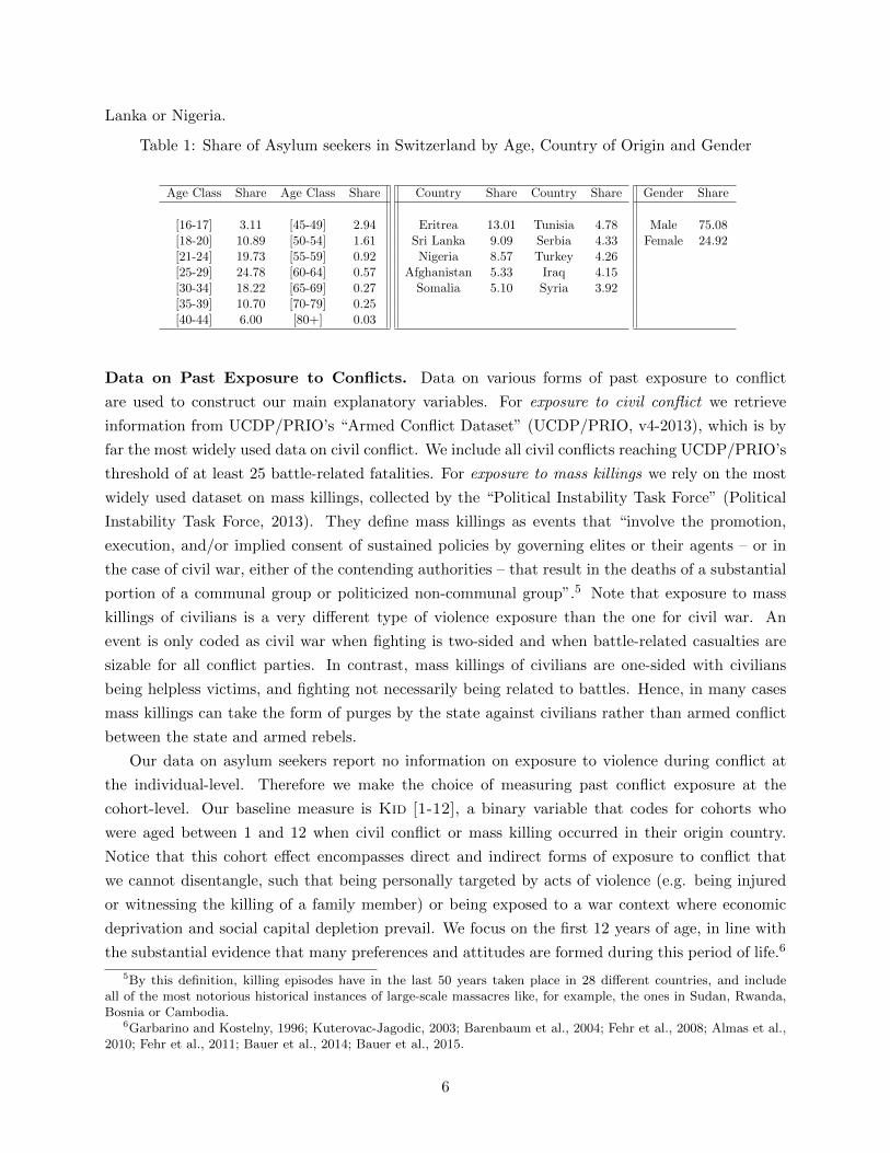
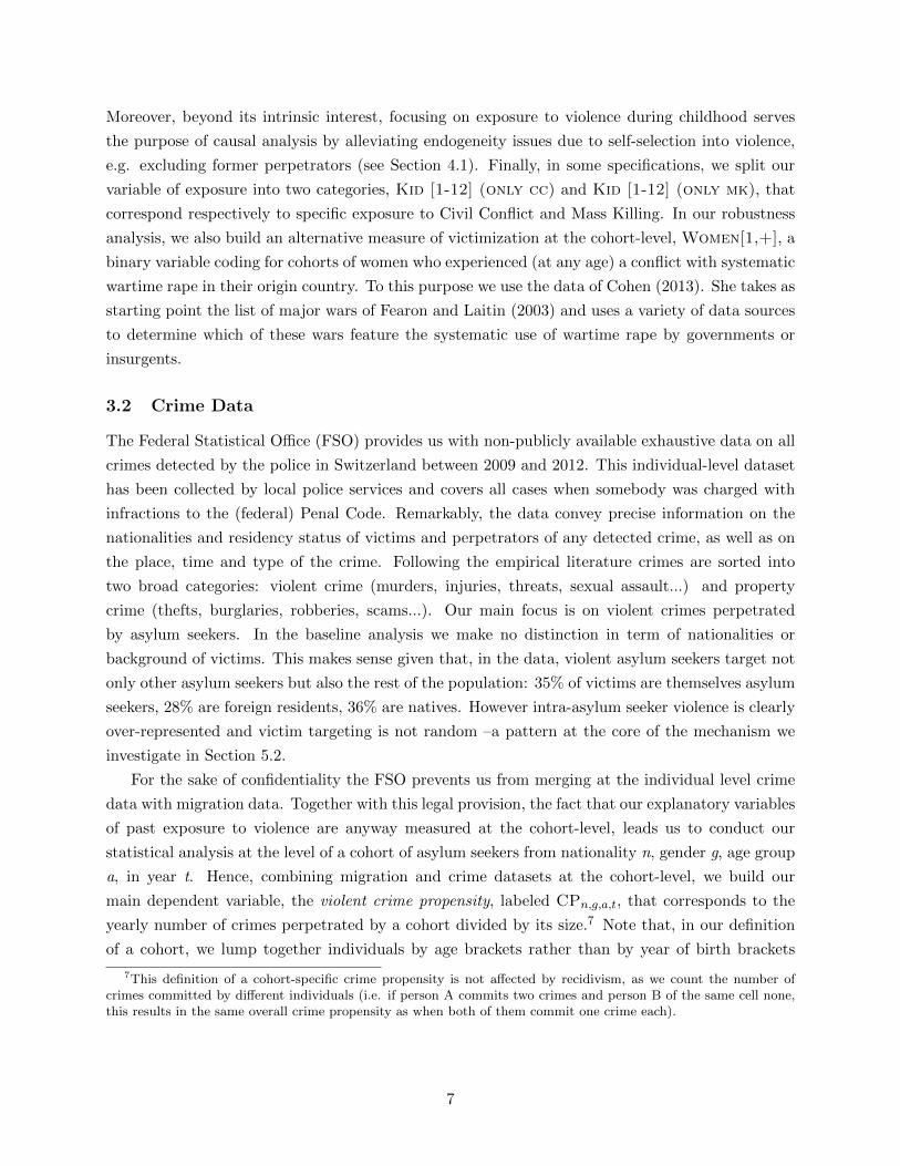
Lanka or Nigeria.

Table 1: Share of Asylum seekers in Switzerland by Age, Country of Origin and Gender

Age Class Share Age Class Share

[16-17] 3.11 [45-49] 2.94[18-20] 10.89 [50-54] 1.61[21-24] 19.73 [55-59] 0.92[25-29] 24.78 [60-64] 0.57[30-34] 18.22 [65-69] 0.27[35-39] 10.70 [70-79] 0.25[40-44] 6.00 [80+] 0.03

Country Share Country Share

Eritrea 13.01 Tunisia 4.78Sri Lanka 9.09 Serbia 4.33Nigeria 8.57 Turkey 4.26

Afghanistan 5.33 Iraq 4.15Somalia 5.10 Syria 3.92

Gender Share

Male 75.08Female 24.92

Data on Past Exposure to Conflicts. Data on various forms of past exposure to conflict

are used to construct our main explanatory variables. For exposure to civil conflict we retrieve

information from UCDP/PRIO’s “Armed Conflict Dataset” (UCDP/PRIO, v4-2013), which is by

far the most widely used data on civil conflict. We include all civil conflicts reaching UCDP/PRIO’s

threshold of at least 25 battle-related fatalities. For exposure to mass killings we rely on the most

widely used dataset on mass killings, collected by the “Political Instability Task Force” (Political

Instability Task Force, 2013). They define mass killings as events that “involve the promotion,

execution, and/or implied consent of sustained policies by governing elites or their agents – or in

the case of civil war, either of the contending authorities – that result in the deaths of a substantial

portion of a communal group or politicized non-communal group”.5 Note that exposure to mass

killings of civilians is a very different type of violence exposure than the one for civil war. An

event is only coded as civil war when fighting is two-sided and when battle-related casualties are

sizable for all conflict parties. In contrast, mass killings of civilians are one-sided with civilians

being helpless victims, and fighting not necessarily being related to battles. Hence, in many cases

mass killings can take the form of purges by the state against civilians rather than armed conflict

between the state and armed rebels.

Our data on asylum seekers report no information on exposure to violence during conflict at

the individual-level. Therefore we make the choice of measuring past conflict exposure at the

cohort-level. Our baseline measure is Kid [1-12], a binary variable that codes for cohorts who

were aged between 1 and 12 when civil conflict or mass killing occurred in their origin country.

Notice that this cohort effect encompasses direct and indirect forms of exposure to conflict that

we cannot disentangle, such that being personally targeted by acts of violence (e.g. being injured

or witnessing the killing of a family member) or being exposed to a war context where economic

deprivation and social capital depletion prevail. We focus on the first 12 years of age, in line with

the substantial evidence that many preferences and attitudes are formed during this period of life.6

5By this definition, killing episodes have in the last 50 years taken place in 28 different countries, and includeall of the most notorious historical instances of large-scale massacres like, for example, the ones in Sudan, Rwanda,Bosnia or Cambodia.

6Garbarino and Kostelny, 1996; Kuterovac-Jagodic, 2003; Barenbaum et al., 2004; Fehr et al., 2008; Almas et al.,2010; Fehr et al., 2011; Bauer et al., 2014; Bauer et al., 2015.

6

Moreover, beyond its intrinsic interest, focusing on exposure to violence during childhood serves

the purpose of causal analysis by alleviating endogeneity issues due to self-selection into violence,

e.g. excluding former perpetrators (see Section 4.1). Finally, in some specifications, we split our

variable of exposure into two categories, Kid [1-12] (only cc) and Kid [1-12] (only mk), that

correspond respectively to specific exposure to Civil Conflict and Mass Killing. In our robustness

analysis, we also build an alternative measure of victimization at the cohort-level, Women[1,+], a

binary variable coding for cohorts of women who experienced (at any age) a conflict with systematic

wartime rape in their origin country. To this purpose we use the data of Cohen (2013). She takes as

starting point the list of major wars of Fearon and Laitin (2003) and uses a variety of data sources

to determine which of these wars feature the systematic use of wartime rape by governments or

insurgents.

3.2 Crime Data

The Federal Statistical Office (FSO) provides us with non-publicly available exhaustive data on all

crimes detected by the police in Switzerland between 2009 and 2012. This individual-level dataset

has been collected by local police services and covers all cases when somebody was charged with

infractions to the (federal) Penal Code. Remarkably, the data convey precise information on the

nationalities and residency status of victims and perpetrators of any detected crime, as well as on

the place, time and type of the crime. Following the empirical literature crimes are sorted into

two broad categories: violent crime (murders, injuries, threats, sexual assault...) and property

crime (thefts, burglaries, robberies, scams...). Our main focus is on violent crimes perpetrated

by asylum seekers. In the baseline analysis we make no distinction in term of nationalities or

background of victims. This makes sense given that, in the data, violent asylum seekers target not

only other asylum seekers but also the rest of the population: 35% of victims are themselves asylum

seekers, 28% are foreign residents, 36% are natives. However intra-asylum seeker violence is clearly

over-represented and victim targeting is not random –a pattern at the core of the mechanism we

investigate in Section 5.2.

For the sake of confidentiality the FSO prevents us from merging at the individual level crime

data with migration data. Together with this legal provision, the fact that our explanatory variables

of past exposure to violence are anyway measured at the cohort-level, leads us to conduct our

statistical analysis at the level of a cohort of asylum seekers from nationality n, gender g, age group

a, in year t. Hence, combining migration and crime datasets at the cohort-level, we build our

main dependent variable, the violent crime propensity, labeled CPn,g,a,t, that corresponds to the

yearly number of crimes perpetrated by a cohort divided by its size.7 Note that, in our definition

of a cohort, we lump together individuals by age brackets rather than by year of birth brackets

7This definition of a cohort-specific crime propensity is not affected by recidivism, as we count the number ofcrimes committed by different individuals (i.e. if person A commits two crimes and person B of the same cell none,this results in the same overall crime propensity as when both of them commit one crime each).

7

because age is a first-order determinant of criminality.8 Given the short time span of our panel

(2009-2012), these two coding options are in fact very close and they would be identical in the case

of a cross-sectional dataset.

Exhaustive data of such high quality is only available in Switzerland for detection data of

charges for crime, and not for data on final convictions by a court.9 While of course the number of

charges for crime are highly correlated with the number of convictions, there may be discrepancies

if for example in some cantons and years the police authorities are more active and successful than

in others. Such spatial differences in detection probabilities of a crime are however accounted for

by the exogenous allocation of asylum seekers across the Swiss territory (or the inclusion of canton

× year fixed effects in Section 7). There could also be a wedge between crime rates of nationals

and foreigners if for example some police forces were to predominantly control foreign-looking

individuals. This however would not bias our estimation as we restrict ourselves to within-asylum

seeker comparisons and do not compare asylum seeker crime rates with crime rates of Swiss citizens.

3.3 Descriptive Statistics

We observe a total annual number of between 22790 and 32413 asylum seekers from 134 nationalities

over the 2009-2012 period. After aggregating by nationality n, gender g, age group a, for each year t,

this leaves us with 4820 cohorts, which are our units of observation. The average cohort is composed

of 22 individuals. Notice that the variance in cohort size is large (standard deviation equals 63

individuals) and this feature of our micro-data calls for weighting our cohort-level regressions by

the number of individuals in each cohort (see our discussion on grouped data in Section 4).

Table 2 reports the main descriptive statistics for cohorts. Note first that 84% of cohorts

originate from countries that have experienced at least one episode of civil conflict or mass killings

since 1946. Among the 134 nationalities of origins, conflicts occurred in 90 countries, mass killings

in 27 countries, and wartime rape in 46 countries. These nationalities are the ones that contribute

to our identifying variations. All these countries experienced violence in some, but not all years,

leading to within-nationality, inter-cohort variations in exposure to violence: The sample mean

of childhood exposure, Kid [1-12], is equal to 48%. As for our alternative measure of exposure,

Women[1,+], we see that 38% of female cohorts have experienced a conflict where wartime rapes

were pervasive. Finally, note that a substantial part of asylum seekers do not flee their country

during war time, but years or even decades afterwards.10 The average number of years since the

last Civil Conflict/Mass Killing is around 10 years.

8While the exact age is reported for asylum seekers, we have only age brackets for the sample of economic migrants(see Section 7). For the sake of comparison we regroup asylum seekers in similar age brackets, that are 16-17, 18-20,21-24, 25-29, 30-34, 35-39, 40-44, 45-49, 50-54, 55-59, 60-64, 65-69, 70-79, > 80 years old.

9Due to the differences across cantons regarding the judicial procedures and duration of trials, the harmonizationof individual conviction data is very hard and does not currently exist. Moreover, a meaningful harmonization ofconviction data for asylum seekers would be even harder, as in many cases asylum seekers may get expelled beforethe end of the lengthy trial.

1041% of cohorts arrive in Switzerland in a year when active conflict is still raging in their home country. Further,only 2 percent of asylum seekers originate from a country that is coded as experiencing current one-sided mass killings,and 5 percent of female cohorts flee a country that is currently plagued by wartime rape.

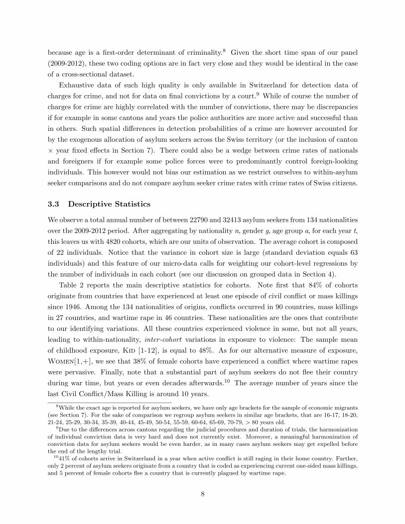
8

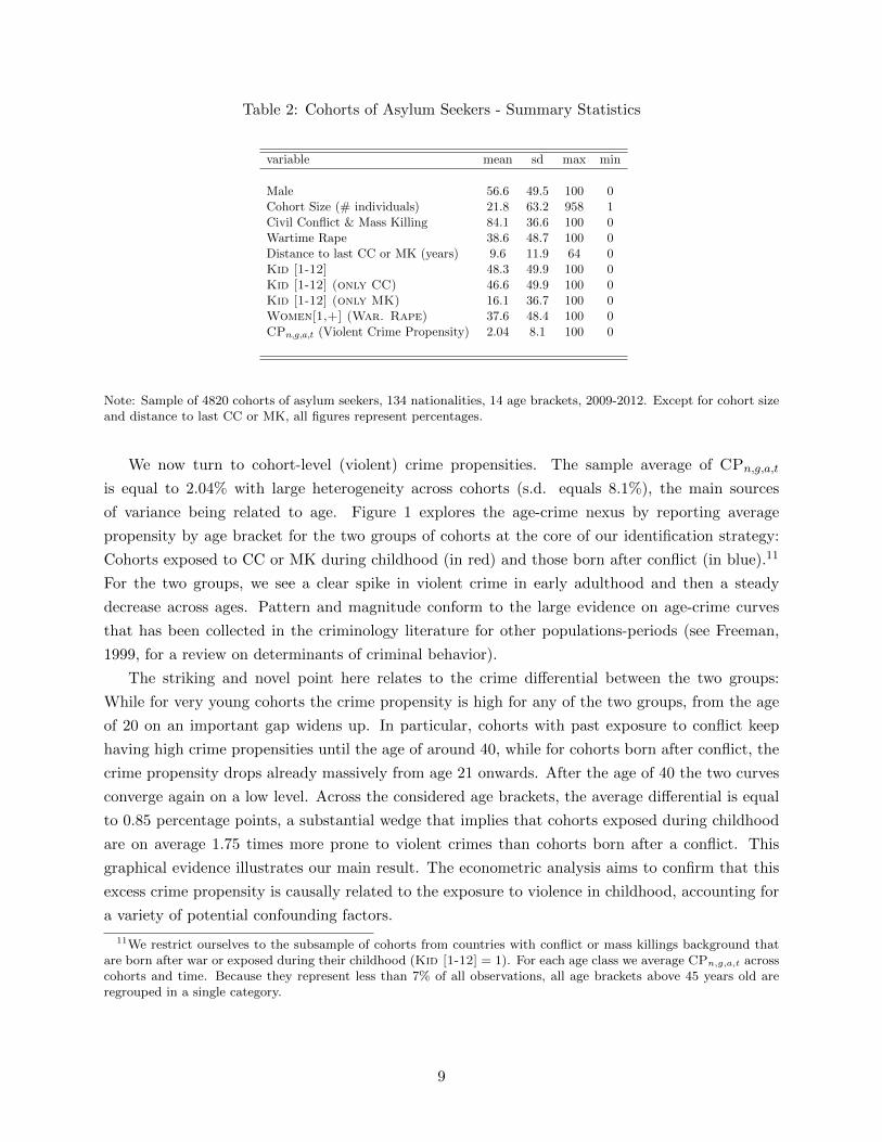
Table 2: Cohorts of Asylum Seekers - Summary Statistics

variable mean sd max min

Male 56.6 49.5 100 0Cohort Size (# individuals) 21.8 63.2 958 1Civil Conflict & Mass Killing 84.1 36.6 100 0Wartime Rape 38.6 48.7 100 0Distance to last CC or MK (years) 9.6 11.9 64 0Kid [1-12] 48.3 49.9 100 0Kid [1-12] (only CC) 46.6 49.9 100 0Kid [1-12] (only MK) 16.1 36.7 100 0Women[1,+] (War. Rape) 37.6 48.4 100 0CPn,g,a,t (Violent Crime Propensity) 2.04 8.1 100 0

Note: Sample of 4820 cohorts of asylum seekers, 134 nationalities, 14 age brackets, 2009-2012. Except for cohort sizeand distance to last CC or MK, all figures represent percentages.

We now turn to cohort-level (violent) crime propensities. The sample average of CPn,g,a,t

is equal to 2.04% with large heterogeneity across cohorts (s.d. equals 8.1%), the main sources

of variance being related to age. Figure 1 explores the age-crime nexus by reporting average

propensity by age bracket for the two groups of cohorts at the core of our identification strategy:

Cohorts exposed to CC or MK during childhood (in red) and those born after conflict (in blue).11

For the two groups, we see a clear spike in violent crime in early adulthood and then a steady

decrease across ages. Pattern and magnitude conform to the large evidence on age-crime curves

that has been collected in the criminology literature for other populations-periods (see Freeman,

1999, for a review on determinants of criminal behavior).

The striking and novel point here relates to the crime differential between the two groups:

While for very young cohorts the crime propensity is high for any of the two groups, from the age

of 20 on an important gap widens up. In particular, cohorts with past exposure to conflict keep

having high crime propensities until the age of around 40, while for cohorts born after conflict, the

crime propensity drops already massively from age 21 onwards. After the age of 40 the two curves

converge again on a low level. Across the considered age brackets, the average differential is equal

to 0.85 percentage points, a substantial wedge that implies that cohorts exposed during childhood

are on average 1.75 times more prone to violent crimes than cohorts born after a conflict. This

graphical evidence illustrates our main result. The econometric analysis aims to confirm that this

excess crime propensity is causally related to the exposure to violence in childhood, accounting for

a variety of potential confounding factors.

11We restrict ourselves to the subsample of cohorts from countries with conflict or mass killings background thatare born after war or exposed during their childhood (Kid [1-12] = 1). For each age class we average CPn,g,a,t acrosscohorts and time. Because they represent less than 7% of all observations, all age brackets above 45 years old areregrouped in a single category.

9

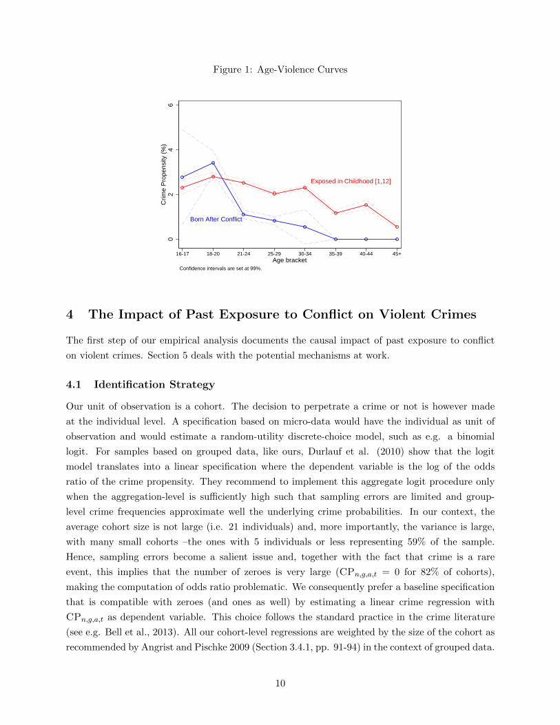
Figure 1: Age-Violence Curves

Exposed in Childhood [1,12]

Born After Conflict

02

46

Crim

e P

rope

nsity

(%

)

16-17 18-20 21-24 25-29 30-34 35-39 40-44 45+Age bracket

Confidence intervals are set at 99%.

4 The Impact of Past Exposure to Conflict on Violent Crimes

The first step of our empirical analysis documents the causal impact of past exposure to conflict

on violent crimes. Section 5 deals with the potential mechanisms at work.

4.1 Identification Strategy

Our unit of observation is a cohort. The decision to perpetrate a crime or not is however made

at the individual level. A specification based on micro-data would have the individual as unit of

observation and would estimate a random-utility discrete-choice model, such as e.g. a binomial

logit. For samples based on grouped data, like ours, Durlauf et al. (2010) show that the logit

model translates into a linear specification where the dependent variable is the log of the odds

ratio of the crime propensity. They recommend to implement this aggregate logit procedure only

when the aggregation-level is sufficiently high such that sampling errors are limited and group-

level crime frequencies approximate well the underlying crime probabilities. In our context, the

average cohort size is not large (i.e. 21 individuals) and, more importantly, the variance is large,

with many small cohorts –the ones with 5 individuals or less representing 59% of the sample.

Hence, sampling errors become a salient issue and, together with the fact that crime is a rare

event, this implies that the number of zeroes is very large (CPn,g,a,t = 0 for 82% of cohorts),

making the computation of odds ratio problematic. We consequently prefer a baseline specification

that is compatible with zeroes (and ones as well) by estimating a linear crime regression with

CPn,g,a,t as dependent variable. This choice follows the standard practice in the crime literature

(see e.g. Bell et al., 2013). All our cohort-level regressions are weighted by the size of the cohort as

recommended by Angrist and Pischke 2009 (Section 3.4.1, pp. 91-94) in the context of grouped data.

10

Our baseline specifications retain analytical weights because the set of covariates is cohort-specific

and our dependent variable (crime propensity) corresponds to the cohort-level average of crime

occurrence across individuals.12 Finally, in the robustness Section 4.4 we investigate alternative

options and econometric specifications for dealing with small cohorts, zeroes/ones, and weighting

schemes.

Our baseline crime regression corresponds to

CPn,g,a,t = α×Kid [1-12]n,a,t +k=80+∑k=13

β(k)× expo(k)n,a,t + FEn,t + FEg + FEa + εn,g,a,t, (1)

where CPn,g,a,t stands for the violent crime propensity of a cohort of nationality (n)× gender(g)×age bracket (a)× year (t). As discussed above, our main explanatory variable is Kid [1-12]n,a,t that

is a binary measure of childhood exposure. The set of control variables expo(k)n,a,t are also binary

variables coding for past exposure, but at the later ages k ∈ {13, 14, 15, ..., 80+}. Hence, in equation

1, the implicit reference group consists of cohorts born after a conflict.13 As a consequence, our

parameter of interest α can be interpreted as the crime differential between cohorts exposed during

their childhood and cohorts born after the conflict. Crucially, the richness of our dataset makes

possible the inclusion of a vast array of fixed effects that account for unobserved heterogeneity in

nationality×year (FEn,t), in age (FEa) and in gender (FEg). Finally, robust standard errors are

clustered at the nationality × year level. We discuss now in more details the potential econometric

pitfalls.

Spatial sorting in Switzerland – A first challenge relates to the fact that crime-prone

individuals tend to self-select into a crime-facilitating environment. For example, individuals

exposed to conflict in their origin country are used to live in areas with high economic depri-

vation and violence; by contrast, individuals from peaceful background, once in Switzerland,

could strategically avoid criminal hotspots or poorest neighborhoods with few labor market

opportunities. This example illustrates a case where past exposure to conflict correlates with

an unobserved cohort characteristic (i.e. preferences in terms of living area) that impacts

crime-proneness in Switzerland.

Our empirical strategy is able to rule out this spatial sorting issue by restricting our core

estimates to asylum seekers, a subsample of migrants who are exogenously allocated across

Switzerland (see Section 4.2). Notice that this exogenous allocation has a second virtue

related to the fact that cantons are very heterogeneous in term of pro-asylum policies which

may affect the elasticity of violence propensity to past conflict exposure. The exogenous

12In Section 4.4 we show that the exact choice of the weighting procedure (analytical, frequency or probability)has a limited impact on the estimated standard deviations.

13We code expo(k)n,a,t = 1 for cohorts who were aged k years old when civil conflict or mass killings occurred intheir origin country. A cohort could be exposed at different periods of life. Cohorts that are born after the last yearof conflict in their origin country are considered as born after. The last year of conflict is defined as the last year ofconflict over all the years of conflict in a country.

11

allocation makes sure that exposed individuals cannot select location according to cantonal

policies.

Pre-conflict characteristics of origin countries – Our empirical analysis intends to cap-

ture the consequences of past conflict exposure on crime propensity. We consequently include

nationality fixed effects (captured by FEn,t), in order to filter out slow-moving characteristics

of the origin country that could correlate with frequent war outbreaks and crime-promoting

characteristics (weak institutions, low social capital and dismal inter-ethnic trust, etc.).

Selection into migration – The push and pull factors determining migration decisions

are likely to be affected by conflicts. Presumably, peacetime is associated to economic mi-

gration while humanitarian migrants are over-represented in post-conflict periods. In turn,

this could affect post-migration crime incentives in the destination country. The inclusion

of gender and age bracket fixed effects, FEg and FEa, aims to control for the main socio-

demographic co-determinants of violent behaviors and the decision to emigrate. Further, at

least as important is the inclusion of the nationality×years fixed effects (FEn,t) which absorb

time-series variations in origin-specific push factors.

Note that we have no information on the educational level of asylum seekers. Therefore

the estimated excess criminality of exposed cohorts could be partly linked to unobserved

heterogeneity in human capital. In our baseline specifications we do not want to control for

this channel because we believe that economic deprivation and educational disruption are

important drivers of the causal impact of past exposure to conflict on violent criminality.

However, when we study the specific channel of intra-national grievances in Section 5.2 we

control for education and human capital thanks to the inclusion of cohort-specific fixed effects

(in bilateral crime regressions).

Perpetrators and victims – Related to the previous point, it could be that after a con-

flict perpetrators are over-represented among migration waves. Hence, high crime proneness

in Switzerland may not only be due to participation to the war, but to prewar individual

disposition. To alleviate this concern we exclude the potential perpetrators by focusing on

the sub-sample of victims exclusively, i.e. i/ individuals who were children during the war

compared to those born afterwards; ii/women born before the war compared to those born

afterwards.

All in all, we deal with a demanding empirical strategy: Our source of identification corresponds

to variations in crime-propensities across cohorts of asylum seekers from the same nationality,

gender and migration wave but with different exposure to conflict (i.e. born after war/exposed in

childhood). Because these cohorts inevitably differ in terms of age, we must control for the direct

effect of age by comparing them to other cohorts with similar age structure but born after a conflict

in another country. To give an example, our strategy consists of computing the crime differential

of two Rwandese cohorts, one born in 1996 (born after the 1994 genocide), and one born in 1990

12

(exposed during childhood), migrating to Switzerland in 2012. In order to control for age-crime

effects, their crime differential is compared to the one of two Nigerian cohorts of same ages but

both being born (in 1990 and 1996) after the 1967-1970 civil war. Our comparison of the blue and

red crime-age curves in Figure 1, panel (a), follows the same logic.

Thus, our strategy is basically akin to a difference-in-difference in country × cohort.14 The

identifying assumption is that past exposure to conflict is the only reason why the decline in crime

rates with age is smaller for asylum seekers exposed in childhood than for their co-nationals born

after. A threat to our identification strategy would be that post-war contexts are systematically

associated to a flattening of the age-crime curve for all cohorts. With this respect, a reassuring fact

is the robustness of our results when all nationalities with no recent history of conflict are excluded

from the sample (columns 3 to 5 in the baseline Table 3). In this case all in-sample cohorts have

been exposed to a conflict or to a post-conflict context: The control group itself being composed of

cohorts born after a conflict, the diff-in-diff results cannot be driven by a war-induced flattening of

the age-crime curve for all cohorts. Another reassuring pattern is the observation in Table 5 of a

sharp decrease in crime propensity between cohorts born during conflicts and those born just after.

Finally, we explore further this question in Section 4.4. Among other validity checks, we perform a

Monte Carlo (placebo) test based on cross-cohorts counterfactual reassignments of conflict exposure

during childhood.

4.2 Exogenous Spatial Allocation of Asylum Seekers in Switzerland

We now provide an overview of the actual process of allocation of asylum seekers across Swiss

cantons. We also discuss briefly some statistical evidence supporting the view that the distribution

key is based on canton population size only and is exogenous to migrants’ characteristics. Many

more details on the institutional/legal aspects and on the formal statistical tests are provided in

Appendices C and D respectively.

Overview of the allocation process– Most asylum seekers enter Switzerland illegally (especially

crossing the Italian border) and apply for asylum in one of the four national reception and procedure

centers (RPC). In the RPC, asylum seekers go through interviews, where they are asked to provide

identity proofs, fingerprints, and their application reasons. During the lengthy assessment process,

the credible asylum seekers are granted a temporary N permit by the Swiss authorities. Given

the difficulty in assessing the threat of persecution in the home country and the large number of

applicants (around 25 000 per year over the 2009-2010 period), the asylum process takes substantial

time. Between 2009-2010, the average duration of the process was 300-400 days, with complex cases

taking several years.

Crucially, during this period holders of the N-permit are exogenously allocated to cantons and

are not allowed to change canton. The allocation of new N-permit holders to the 26 Swiss cantons is

determined by a exogenous allocation key based on the cantonal population. Once an asylum seeker

14We thank Christian Dustmann and Erzo Luttmer for their comments and suggestions on this point.

13

has been allocated to a given canton, the canton in charge organizes the accommodation in cantonal

centers or flats and takes care of the interviews and of financial matters. This allocation rule was

introduced in the amendment to the Aliens Law in 1988, presumably to minimize self-segregation

and ghetto effects and avoid social tensions between natives and asylum seekers.

The allocation is made by the Federal Office for Migration in Bern and its decision cannot be

appealed unless under certain precise conditions (family unity reasons like minors being allocated

to a different canton than their parents or if the asylum seeker or a third person are under serious

threat) and the change of the canton is possible only if the two cantons approve it. According to

Hofmann and Buchmann (2008), it is extremely rare that asylum seekers change canton or cantons

refuse asylum seekers.

Statistical Evidence– Figure 2 in the Appendix displays the time series evolution of asylum seeker

stocks across the 26 Swiss cantons between 1994-2010 (the main peak corresponding to the end

of the Kosovo war). Visual inspection confirms parallel trends across cantons and this constitutes

a first and rough piece of evidence consistent with an exogenous allocation process of migrants

across cantons. More substantially, we provide formal statistical tests in Table 21 of Appendix D.

The purpose is to tackle the question of whether there is indeed an exogenous allocation of asylum

seekers following the official population-based distribution key –as we claim– or if there may be

some selection on relevant dimensions. The basic approach consists in testing for the difference

in means between cantons for various observable cohort characteristics (i.e. exposure to violence

during childhood, age, gender). We first perform this test for each nationality of asylum seekers.

However, a concern is that, for small nationality sizes, sampling variations mechanically lead to

observed patterns of spatial concentration in some cantons. A first attempt to tackle this sampling

issue consists in pooling cohorts from all nationalities by year. A second attempt corresponds to a

Monte Carlo simulation (1000 draws) generating artificial random allocations that we compare to

the observed allocation. Overall, the tests of Table 21 are supportive of our identifying assumption

that the allocation of asylum seekers across cantons can be considered as exogenous with respect

to their age, gender and past exposure to violence.

4.3 Baseline Results

Table 3 displays the baseline estimation results of our cohort-level crime regression (equation 1).

We report only our coefficient of interest, α, that captures the impact on violent crime propen-

sity of cohorts exposed to civil war or mass killings during childhood (1-12 years), the reference

group being cohorts born after conflict. Column 1 reports the results of a pooled regression with

age and gender fixed effects but without country × year fixed effects. The coefficient of interest

is positive and significant at the 5 percent threshold. However, as explained in Section 4.1 this

correlation is potentially driven by confounding factors that relate to pre-conflict characteristics

of origin countries or by selection into migration. In Column 2, we consider a specification with

the full battery of fixed effects where the identifying variations come from within-nationality /

14

between-cohorts comparison. This is our preferred specification (baseline). The coefficient of past

exposure is reduced by one third but it retains statistical significance and a positive sign. In term of

magnitude, we observe that the crime propensity of cohorts exposed during childhood is on average

0.83 percentage points higher than the propensity of their co-national cohorts born after the war –a

substantial effect given that the sample mean of violent crime propensity is equal to 2.04 percentage

points. By means of benchmarks, gender and age have comparable consequences on crime propen-

sity. The non-reported coefficient of the male dummy (reference group being female) is 3.03. This

is not surprising, as it is widely known that most violent crimes are perpetrated by men. But the

striking point is that exposure to conflict has an impact of the same order of magnitude, although

smaller (about one fourth). Also age matters (coefficients are not reported here): the 16-17 years

old have 6.5 percentage points, the 18-20 years old have 5.95 percentage points, 21-24 years old

4.8 percentage points and 25-29 years old 3.5 percentage points higher crime propensity than the

cohort being more than 50 years old. In a nutshell, even if gender and age tend to be powerful

determinants of crime, past exposure to conflict in childhood still substantially matters. In column

3 we exclude all cohorts originating from countries that have experienced no civil conflict or mass

killing since 1946. The point estimate is barely changed in spite of the sample size reduction. In

columns 4 and 5 we estimate the same specification as in column 3, but now separately for conflict

and mass killings. In each case, the sample is again restricted to countries having experienced each

specific type of violence.

Heterogeneous Effects: Gender and Type of Crime – In Table 4 we study heterogeneous

effects with respect to gender and type of crime. Columns 1 and 2 replicate our baseline specifica-

tion (Column 2 of Table 3) on the subsamples of male and female cohorts respectively. The results

are clearly driven by men, with the coefficient for women being of smaller size and not statistically

significant. Columns 3 to 5 focus on the propensity to property crime instead of violent crime

as dependent variable, respectively for the full sample, for men only and for women only. The

magnitude and the statistical significance of our variable of interest is strikingly lower, suggesting

that exposure to conflict during childhood impacts future violent behaviors, but leaves future non-

violent criminality unaffected. We see this contrasted evidence as a first indication that our causal

effect captures a mechanism of perpetuation of violence –a point that we develop in more detail in

Section 5. From the perspective of causal analysis we interpret the absence of effect for property

crime as an indication that the correlation between past exposure and violent crime is unlikely

to be spuriously driven by omitted factors (unless such factors were to affect differentially violent

crimes and property crimes).

Heterogeneous Effects: Age – Table 5 is also devoted to heterogeneous effects, with a special

focus on age. In Column 1, we are interested in lifecycle modulations of the impact of past exposure.

We interact our main explanatory variable with (mutually exclusive) decade dummies coding for

the current age of the cohorts. We see no significant difference for exposed and non-exposed

15

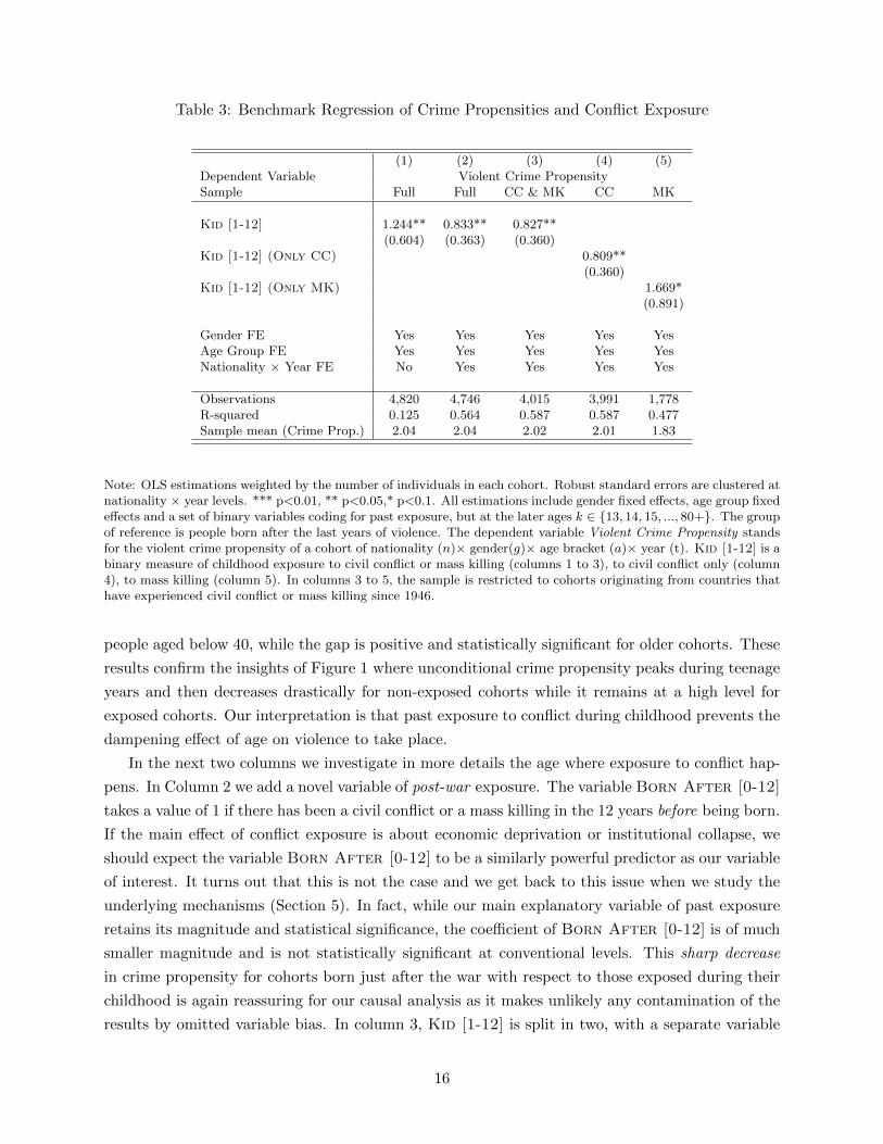
Table 3: Benchmark Regression of Crime Propensities and Conflict Exposure

(1) (2) (3) (4) (5)Dependent Variable Violent Crime PropensitySample Full Full CC & MK CC MK

Kid [1-12] 1.244** 0.833** 0.827**(0.604) (0.363) (0.360)

Kid [1-12] (Only CC) 0.809**(0.360)

Kid [1-12] (Only MK) 1.669*(0.891)

Gender FE Yes Yes Yes Yes YesAge Group FE Yes Yes Yes Yes YesNationality × Year FE No Yes Yes Yes Yes

Observations 4,820 4,746 4,015 3,991 1,778R-squared 0.125 0.564 0.587 0.587 0.477Sample mean (Crime Prop.) 2.04 2.04 2.02 2.01 1.83

Note: OLS estimations weighted by the number of individuals in each cohort. Robust standard errors are clustered atnationality × year levels. *** p<0.01, ** p<0.05,* p<0.1. All estimations include gender fixed effects, age group fixedeffects and a set of binary variables coding for past exposure, but at the later ages k ∈ {13, 14, 15, ..., 80+}. The groupof reference is people born after the last years of violence. The dependent variable Violent Crime Propensity standsfor the violent crime propensity of a cohort of nationality (n)× gender(g)× age bracket (a)× year (t). Kid [1-12] is abinary measure of childhood exposure to civil conflict or mass killing (columns 1 to 3), to civil conflict only (column4), to mass killing (column 5). In columns 3 to 5, the sample is restricted to cohorts originating from countries thathave experienced civil conflict or mass killing since 1946.

people aged below 40, while the gap is positive and statistically significant for older cohorts. These

results confirm the insights of Figure 1 where unconditional crime propensity peaks during teenage

years and then decreases drastically for non-exposed cohorts while it remains at a high level for

exposed cohorts. Our interpretation is that past exposure to conflict during childhood prevents the

dampening effect of age on violence to take place.

In the next two columns we investigate in more details the age where exposure to conflict hap-

pens. In Column 2 we add a novel variable of post-war exposure. The variable Born After [0-12]

takes a value of 1 if there has been a civil conflict or a mass killing in the 12 years before being born.

If the main effect of conflict exposure is about economic deprivation or institutional collapse, we

should expect the variable Born After [0-12] to be a similarly powerful predictor as our variable

of interest. It turns out that this is not the case and we get back to this issue when we study the

underlying mechanisms (Section 5). In fact, while our main explanatory variable of past exposure

retains its magnitude and statistical significance, the coefficient of Born After [0-12] is of much

smaller magnitude and is not statistically significant at conventional levels. This sharp decrease

in crime propensity for cohorts born just after the war with respect to those exposed during their

childhood is again reassuring for our causal analysis as it makes unlikely any contamination of the

results by omitted variable bias. In column 3, Kid [1-12] is split in two, with a separate variable

16

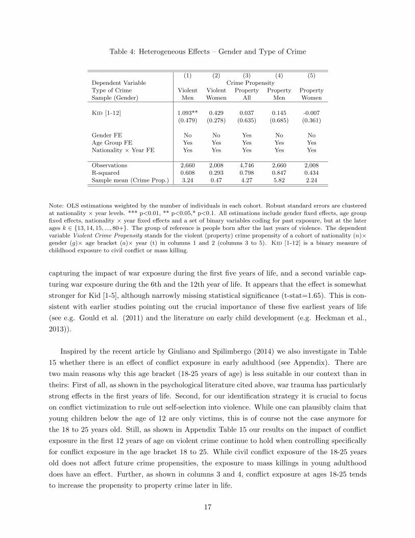
Table 4: Heterogeneous Effects – Gender and Type of Crime

(1) (2) (3) (4) (5)Dependent Variable Crime PropensityType of Crime Violent Violent Property Property PropertySample (Gender) Men Women All Men Women

Kid [1-12] 1.093** 0.429 0.037 0.145 -0.007(0.479) (0.278) (0.635) (0.685) (0.361)

Gender FE No No Yes No NoAge Group FE Yes Yes Yes Yes YesNationality × Year FE Yes Yes Yes Yes Yes

Observations 2,660 2,008 4,746 2,660 2,008R-squared 0.608 0.293 0.798 0.847 0.434Sample mean (Crime Prop.) 3.24 0.47 4.27 5.82 2.24

Note: OLS estimations weighted by the number of individuals in each cohort. Robust standard errors are clusteredat nationality × year levels. *** p<0.01, ** p<0.05,* p<0.1. All estimations include gender fixed effects, age groupfixed effects, nationality × year fixed effects and a set of binary variables coding for past exposure, but at the laterages k ∈ {13, 14, 15, ..., 80+}. The group of reference is people born after the last years of violence. The dependentvariable Violent Crime Propensity stands for the violent (property) crime propensity of a cohort of nationality (n)×gender (g)× age bracket (a)× year (t) in columns 1 and 2 (columns 3 to 5). Kid [1-12] is a binary measure ofchildhood exposure to civil conflict or mass killing.

capturing the impact of war exposure during the first five years of life, and a second variable cap-

turing war exposure during the 6th and the 12th year of life. It appears that the effect is somewhat

stronger for Kid [1-5], although narrowly missing statistical significance (t-stat=1.65). This is con-

sistent with earlier studies pointing out the crucial importance of these five earliest years of life

(see e.g. Gould et al. (2011) and the literature on early child development (e.g. Heckman et al.,

2013)).

Inspired by the recent article by Giuliano and Spilimbergo (2014) we also investigate in Table

15 whether there is an effect of conflict exposure in early adulthood (see Appendix). There are

two main reasons why this age bracket (18-25 years of age) is less suitable in our context than in

theirs: First of all, as shown in the psychological literature cited above, war trauma has particularly

strong effects in the first years of life. Second, for our identification strategy it is crucial to focus

on conflict victimization to rule out self-selection into violence. While one can plausibly claim that

young children below the age of 12 are only victims, this is of course not the case anymore for

the 18 to 25 years old. Still, as shown in Appendix Table 15 our results on the impact of conflict

exposure in the first 12 years of age on violent crime continue to hold when controlling specifically

for conflict exposure in the age bracket 18 to 25. While civil conflict exposure of the 18-25 years

old does not affect future crime propensities, the exposure to mass killings in young adulthood

does have an effect. Further, as shown in columns 3 and 4, conflict exposure at ages 18-25 tends

to increase the propensity to property crime later in life.

17

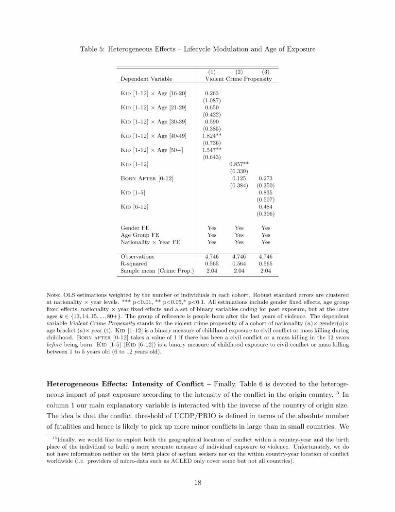
Table 5: Heterogeneous Effects – Lifecycle Modulation and Age of Exposure

(1) (2) (3)Dependent Variable Violent Crime Propensity

Kid [1-12] × Age [16-20] 0.263(1.087)

Kid [1-12] × Age [21-29] 0.650(0.422)

Kid [1-12] × Age [30-39] 0.590(0.385)

Kid [1-12] × Age [40-49] 1.824**(0.736)

Kid [1-12] × Age [50+] 1.547**(0.643)

Kid [1-12] 0.857**(0.339)

Born After [0-12] 0.125 0.273(0.384) (0.350)

Kid [1-5] 0.835(0.507)

Kid [6-12] 0.484(0.306)

Gender FE Yes Yes YesAge Group FE Yes Yes YesNationality × Year FE Yes Yes Yes

Observations 4,746 4,746 4,746R-squared 0.565 0.564 0.565Sample mean (Crime Prop.) 2.04 2.04 2.04

Note: OLS estimations weighted by the number of individuals in each cohort. Robust standard errors are clusteredat nationality × year levels. *** p<0.01, ** p<0.05,* p<0.1. All estimations include gender fixed effects, age groupfixed effects, nationality × year fixed effects and a set of binary variables coding for past exposure, but at the laterages k ∈ {13, 14, 15, ..., 80+}. The group of reference is people born after the last years of violence. The dependentvariable Violent Crime Propensity stands for the violent crime propensity of a cohort of nationality (n)× gender(g)×age bracket (a)× year (t). Kid [1-12] is a binary measure of childhood exposure to civil conflict or mass killing duringchildhood. Born after [0-12] takes a value of 1 if there has been a civil conflict or a mass killing in the 12 yearsbefore being born. Kid [1-5] (Kid [6-12]) is a binary measure of childhood exposure to civil conflict or mass killingbetween 1 to 5 years old (6 to 12 years old).

Heterogeneous Effects: Intensity of Conflict – Finally, Table 6 is devoted to the heteroge-

neous impact of past exposure according to the intensity of the conflict in the origin country.15 In

column 1 our main explanatory variable is interacted with the inverse of the country of origin size.

The idea is that the conflict threshold of UCDP/PRIO is defined in terms of the absolute number

of fatalities and hence is likely to pick up more minor conflicts in large than in small countries. We

15Ideally, we would like to exploit both the geographical location of conflict within a country-year and the birthplace of the individual to build a more accurate measure of individual exposure to violence. Unfortunately, we donot have information neither on the birth place of asylum seekers nor on the within country-year location of conflictworldwide (i.e. providers of micro-data such as ACLED only cover some but not all countries).

18

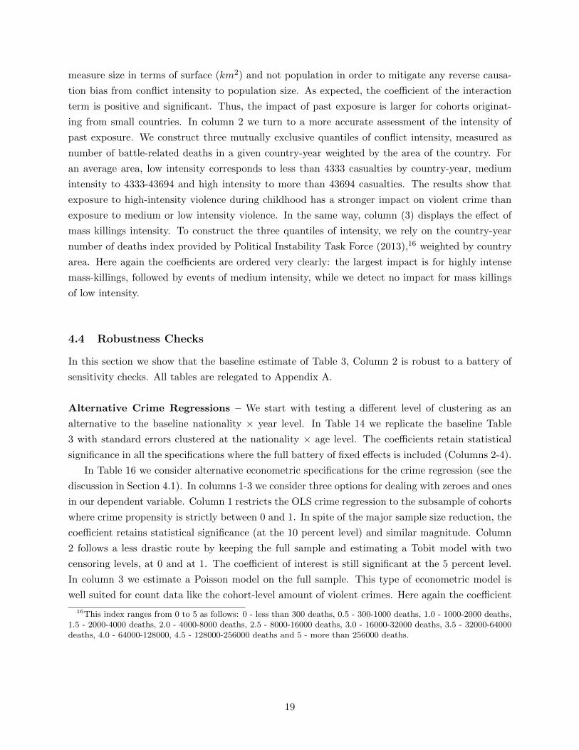
measure size in terms of surface (km2) and not population in order to mitigate any reverse causa-

tion bias from conflict intensity to population size. As expected, the coefficient of the interaction

term is positive and significant. Thus, the impact of past exposure is larger for cohorts originat-

ing from small countries. In column 2 we turn to a more accurate assessment of the intensity of

past exposure. We construct three mutually exclusive quantiles of conflict intensity, measured as

number of battle-related deaths in a given country-year weighted by the area of the country. For

an average area, low intensity corresponds to less than 4333 casualties by country-year, medium

intensity to 4333-43694 and high intensity to more than 43694 casualties. The results show that

exposure to high-intensity violence during childhood has a stronger impact on violent crime than

exposure to medium or low intensity violence. In the same way, column (3) displays the effect of

mass killings intensity. To construct the three quantiles of intensity, we rely on the country-year

number of deaths index provided by Political Instability Task Force (2013),16 weighted by country

area. Here again the coefficients are ordered very clearly: the largest impact is for highly intense

mass-killings, followed by events of medium intensity, while we detect no impact for mass killings

of low intensity.

4.4 Robustness Checks

In this section we show that the baseline estimate of Table 3, Column 2 is robust to a battery of

sensitivity checks. All tables are relegated to Appendix A.

Alternative Crime Regressions – We start with testing a different level of clustering as an

alternative to the baseline nationality × year level. In Table 14 we replicate the baseline Table

3 with standard errors clustered at the nationality × age level. The coefficients retain statistical

significance in all the specifications where the full battery of fixed effects is included (Columns 2-4).

In Table 16 we consider alternative econometric specifications for the crime regression (see the

discussion in Section 4.1). In columns 1-3 we consider three options for dealing with zeroes and ones

in our dependent variable. Column 1 restricts the OLS crime regression to the subsample of cohorts

where crime propensity is strictly between 0 and 1. In spite of the major sample size reduction, the

coefficient retains statistical significance (at the 10 percent level) and similar magnitude. Column

2 follows a less drastic route by keeping the full sample and estimating a Tobit model with two

censoring levels, at 0 and at 1. The coefficient of interest is still significant at the 5 percent level.

In column 3 we estimate a Poisson model on the full sample. This type of econometric model is

well suited for count data like the cohort-level amount of violent crimes. Here again the coefficient

16This index ranges from 0 to 5 as follows: 0 - less than 300 deaths, 0.5 - 300-1000 deaths, 1.0 - 1000-2000 deaths,1.5 - 2000-4000 deaths, 2.0 - 4000-8000 deaths, 2.5 - 8000-16000 deaths, 3.0 - 16000-32000 deaths, 3.5 - 32000-64000deaths, 4.0 - 64000-128000, 4.5 - 128000-256000 deaths and 5 - more than 256000 deaths.

19

Table 6: Heterogeneous Effects – Intensity of Conflict

(1) (2) (3)Dep. Var. Violent Crime PropensityExposure to CC and MK CC MKSample Restricted Restricted Restricted

Kid [1-12] 0.685*(0.389)

Kid [1-12] × 1/(Size) 0.128**(0.057)

Kid [1-12] : low intensity 0.211 -0.369(0.272) (0.387)

Kid [1-12] : medium intensity 1.534* 1.488*(0.844) (0.831)

Kid [1-12] : high intensity 1.856** 2.775*(0.926) (1.411)

Gender FE Yes Yes YesAge Group FE Yes Yes YesNationality × Year FE Yes Yes Yes

Observations 3,991 3,991 1,778R-squared 0.587 0.593 0.483Sample mean (Crime Prop.) 2.01 2.01 1.83

Note: OLS estimations weighted by the number of individuals in each cohort. Robust standard errors are clusteredat nationality × year levels. *** p<0.01, ** p<0.05,* p<0.1. All estimations include gender fixed effects, age groupfixed effects, nationality × year fixed effects and a set of binary variables coding for past exposure, but at the laterages k ∈ {13, 14, 15, ..., 80+}. The group of reference is people born after the last years of violence. The dependentvariable Violent Crime Propensity stands for the violent crime propensity of a cohort of nationality (n)× gender (g)×age bracket (a)× year (t). Kid [1-12] is a binary measure of childhood exposure to civil conflict or mass killing.

is significant with a magnitude comparable to its OLS counterpart.17 Columns 4 and 5 test for

robustness to the removal of outliers. We retrieve from our baseline specification the estimated

residuals. Then we trim the sample to remove all observations for which the residuals are further

away than three standard deviations (column 4) or, even more radically, two standard deviations

(column 5) from the mean residual. In both cases we obtain a statistically significant coefficient at

the 5 percent, resp. 1 percent level; its magnitude is reduced with respect to its baseline counterpart.

In columns 6 and 7 we go back to our baseline specification but change the weighting procedure

of cohorts size by considering probability, resp. frequency weights rather than analytical weights.

In both cases the estimated standard deviations are barely changed with respect to their baseline

counterpart. This stability is likely due to the fact that, irrespective of the weighting scheme, all

specifications estimate a cluster-robust covariance matrix at a level of aggregation higher than the

cohort-level. Column 8 displays the result for the unweighted regression. The magnitude of the

17Note that the estimated standard deviations with the Tobit model have to be considered carefully due to theincidental parameters problem, as the length of our panel is short, T = 4 (Greene, 2004). See Osgood and Wayne(2000) for the use of a poisson-based regression with crime rates.

20

coefficient is comparable to its baseline value; however, it is much less precisely estimated. This

confirms that small cohorts, where crime propensity is more likely to take extreme values (0 or 1),

lead to mismeasurement errors and statistical noise.

Table 17 implements the aggregate logit procedure. It simply consists of an OLS crime regres-

sion where the dependent variable is now the log(odds-ratio) of Crime Propensity, namely ln CP1-CP .

All other features are identical to the baseline specification. As explained in Section 4.1, coping

with (i) zeroes and ones, and (ii) small cohorts, is problematic in such a setting. In column 1 we

replace by CP = 0.001 and CP = 0.999 the observed values of CP that are equal to zero and one

respectively. Though ad-hoc, this coding rule allows to force the definition of the odds-ratio for all

cohorts. In columns 2 and 3 the same coding rule is used but we exclude small cohorts from the

sample (respectively less than 2 individual and less than 3 individuals). Column 4 abstracts from

this coding rule by simply excluding all cohorts with CP = 0 or CP = 1 from the sample. This

leads to a big reduction in sample size. Finally columns 5 and 6 use probability and frequency

weights, respectively, and column 7 displays the result for the unweighted regression. All in all

the coefficient of interest keeps its positive sign. Its magnitude is not directly comparable to its

baseline value due to the logistic transform of the dependent variable. The statistical significance

is slightly reduced (below 10 percent threshold instead of 5 percent in the baseline).

Placebo Test of conflict exposure during childhood– As mentioned in section 4.1, our iden-

tifying assumption is that past exposure to conflict is the only reason why the decline in crime

rates with age is smaller for asylum seekers exposed in childhood than for asylum seekers from the

same nationality and born after the war. With this respect, a reassuring pattern in our data is the

observation in Table 5 of a sharp decrease in crime propensity between cohorts born during conflicts

and those born just after. We now go one step further by performing a falsification exercise based

on a randomization of conflict exposure during childhood. More specifically, we follow a Monte

Carlo approach where we postulate a data generating process that randomly reassigns our main

explanatory variable Kid[1− 12] across cohorts according to a binomial distribution based on the

observed empirical frequencies of 0 and 1. All other cohort characteristics (e.g. nationality, gender,

age) are left unchanged. Then, we estimate the baseline specification (Column 2 of Table 3) on this

fake dataset. This procedure is generated for a large number of realizations (1,000 draws). Figure

3 reports the sampling distribution of the point estimates of the coefficient of Kid[1 − 12] across

the Monte Carlo draws. Visual inspection shows that this distribution is centered around zero and

confirms that the likelihood of spuriously estimating a coefficient equal or above our baseline point

estimate of 0.83 is very small.

Cohort × Canton Sample– The presence of small cohorts potentially leads to sampling vari-

ations in the spatial allocation of Asylum Seekers across Swiss Cantons. Hence, in spite of the

exogenous allocation, cohorts born after conflict could be by chance located in cantons with dif-

ferent characteristics from cohorts born before (see Appendix D). An option for alleviating this

21

concern is to allow for the inclusion of canton × year fixed effects in our econometric model (1).

To this purpose we must disaggregate our cohort-level sample at the canton level. In this case, the

dependent variable becomes CPc,n,g,a,t, the crime propensity of cohort n, g, a, t in canton c. We

replicate the Table 3 in this more fine-grained setting with the additional set of fixed effects and

with the error terms clustered at both nationality × year and canton × year levels. The results

are reported in Table 18. In all columns the coefficient of interest has the expected positive sign

and is most of the time statistically significant. Note however that the R-squared is substantially

smaller, indicating a less good fit of this disaggregated specification.

Alternative Victimization Variable– We now focus on another population group that is often

victimized in conflict, namely women. We know from Table 4 that, on average, childhood exposure

does not impact future violent crime propensity of women. However, it could well be that exposure

to extreme events or to violence targeted specifically towards women does affect the criminality risk

of women. We restrict our sample to female asylum seekers from countries of origins where there

was at least one year of civil war (or mass killing) since 1945 (Table 19). We estimate a version

of equation 1 where the variable of exposure to violence corresponds to Women[1,+]n,a, a binary

variable coded 1 if women from cohort (n, a) have experienced conflict (between birth and residence

in Switzerland) and 0 otherwise. Our identification here is consequently based on the comparison

between women born before the last year of conflict (civil conflict, mass killing or wartime rape,

respectively) and women from the same origin country, born after the last year of conflict (civil

conflict, mass killing or wartime rape, respectively), and being from the same wave of migration.

On the one hand, women exposed to civil conflict or mass killing are not significantly more violent

than women non-exposed (columns 1 to 3, Table 19 in Appendix) but on the other hand women

exposed to a conflict with systematic wartime rape are more crime prone than women who are non

exposed (column 4). From columns 5 to 7, we turn to a more accurate assessment of the intensity

of past exposure, following the same strategy as Table 6. The results indicate that exposure to

high-intensity conflict has a stronger impact on criminal behavior than exposure to medium or low

intensity conflict.

5 Channels of Transmission

Various potential mechanisms contribute to the causal impact of violence exposure on future crime

propensity, the main ones being (i) the psychological trauma of victimization, (ii) the effects of

economic deprivation during war on pervasive developmental disorders or on human capital acqui-

sition and preferences or (iii) societal factors such as the collapse of social capital and altered moral

norms creating lasting grievances towards other groups. While it is challenging to completely rule

out several channels and prove the predominance of others, in this section we take a step in the

direction of evaluating the relative plausibility of possible mechanisms. In particular we emphasize

22

the role of persistence in intra-national grievances.

5.1 Socio-Economic Environment during Childhood

We start in Table 7 by documenting the role of the socio-economic environment during childhood

for conflict-exposed cohorts (see section E in Appendix for more definitions and sources of the

precise variables). In particular, in all uneven columns several control variables are introduced,

while in the following even columns the corresponding regressions are run without the additional

controls, but on the same sample. This allows us to tell apart whether potential changes of the

results are due to the inclusion of control variable or due to a drop in the sample size.

In column 1 we control for the average percentage of people with access to primary schooling

in the years when the underlying individuals in our study were aged younger than 12 years.18 Put

differently, this variable is constructed analogously to our conflict exposure measures, but now

focusing on the exposure to primary education. Column 2 runs our baseline specification on the

same reduced sample of column 1, but without including the education exposure variable. The

coefficient of interest of Kid [1-12] is almost identical in both columns, and the coefficient of

education exposure is statistically insignificant, pointing out that it is unlikely that most of the

effect of conflict exposure goes through reduced schooling. This result is of special importance

given that we cannot control explicitly for human capital or education level at the cohort-level in

our regressions (our data provide no information on these characteristics).

In columns 3 and 4 the focus lies on democracy scores during the childhood of asylum seekers.

We find that while the average democracy score in the home country during the early childhood

years is not statistically significant, the coefficient of interest of conflict exposure remains significant

at the 5 percent level, and of similar magnitude with and without the democracy exposure control.

In columns 5 to 6 we study whether the impact of conflict exposure may go through experiencing

economic deprivation during early childhood. Focusing on GDP per capita, we detect no impact

of poverty during childhood. However, the coefficient of interest of exposure to conflict, though

positive, loses its statistical significance due to the sample size reduction.

5.2 Targeted Violence and Persistence in Intra-National Grievances

We exploit here a unique feature of our dataset on criminality in Switzerland, namely information

on the nationalities of both perpetrators and victims. We use this source of information to build

bilateral crime propensities documenting the propensity of perpetrators to target co-nationals. This

boils down to comparing for example the propensity of a Rwandese asylum seeker (e.g., Tutsi) to

attack another Rwandese (e.g., Hutu), rather than to attack somebody from another country of

18Note that the available education indicator used here is somewhat coarse: It corresponds to the percentage ofthe population aged above 15 years old with at least primary education. While it of course captures the state of theeducation system in a given year, it is not a specific, precise measure of education exposure of the cohort being ofschooling age, but also reflects the education of older generations.

23

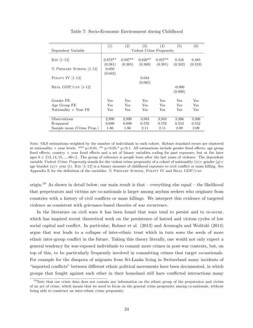
Table 7: Socio-Economic Environment during Childhood

(1) (2) (3) (4) (5) (6)Dependent Variable Violent Crime Propensity

Kid [1-12] 0.873** 0.937** 0.820** 0.857** 0.416 0.485(0.381) (0.385) (0.369) (0.391) (0.342) (0.319)

% Primary School [1-12] 0.050(0.042)

Polity IV [1-12] 0.043(0.065)

Real GDP/cap [1-12] -0.000(0.000)

Gender FE Yes Yes Yes Yes Yes YesAge Group FE Yes Yes Yes Yes Yes YesNationality × Year FE Yes Yes Yes Yes Yes Yes

Observations 2,990 2,990 3,983 3,983 3,396 3,396R-squared 0.699 0.698 0.576 0.576 0.553 0.552Sample mean (Crime Prop.) 1.86 1.86 2.11 2.11 2.09 2.09

Note: OLS estimations weighted by the number of individuals in each cohort. Robust standard errors are clusteredat nationality × year levels. *** p<0.01, ** p<0.05,* p<0.1. All estimations include gender fixed effects, age groupfixed effects, country × year fixed effects and a set of binary variables coding for past exposure, but at the laterages k ∈ {13, 14, 15, ..., 80+}. The group of reference is people born after the last years of violence. The dependentvariable Violent Crime Propensity stands for the violent crime propensity of a cohort of nationality (n)× gender (g)×age bracket (a)× year (t). Kid [1-12] is a binary measure of childhood exposure to civil conflict or mass killing. SeeAppendix E for the definition of the variables: % Primary School, Polity IV and Real GDP/cap.

origin.19 As shown in detail below, our main result is that – everything else equal – the likelihood

that perpetrators and victims are co-nationals is larger among asylum seekers who originate from

countries with a history of civil conflicts or mass killings. We interpret this evidence of targeted

violence as consistent with grievance-based theories of war recurrence.

In the literature on civil wars it has been found that wars tend to persist and to re-occur,

which has inspired recent theoretical work on the persistence of hatred and vicious cycles of low

social capital and conflict. In particular, Rohner et al. (2013) and Acemoglu and Wolitzki (2014)

argue that war leads to a collapse of inter-ethnic trust which in turn sows the seeds of more

ethnic inter-group conflict in the future. Taking this theory literally, one would not only expect a

general tendency for war-exposed individuals to commit more crimes in post-war contexts, but, on

top of this, to be particularly frequently involved in committing crimes that target co-nationals.

For example for the diaspora of migrants from Sri-Lanka living in Switzerland many incidents of

“imported conflicts” between different ethnic political movements have been documented, in which

groups that fought against each other in their homeland still have conflicted interactions many

19Note that our crime data does not contain any information on the ethnic group of the perpetrator and victimof an act of crime, which means that we need to focus on the general crime propensity among co-nationals, withoutbeing able to construct an inter-ethnic crime propensity.

24

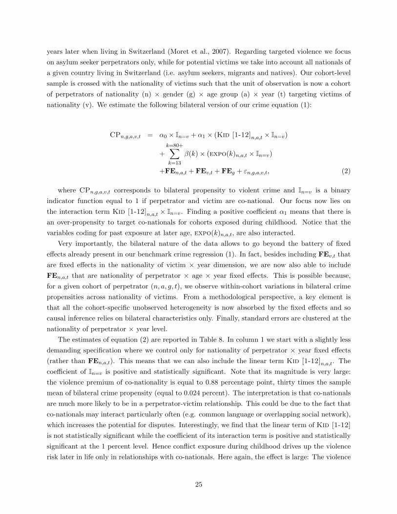
years later when living in Switzerland (Moret et al., 2007). Regarding targeted violence we focus

on asylum seeker perpetrators only, while for potential victims we take into account all nationals of

a given country living in Switzerland (i.e. asylum seekers, migrants and natives). Our cohort-level

sample is crossed with the nationality of victims such that the unit of observation is now a cohort

of perpetrators of nationality (n) × gender (g) × age group (a) × year (t) targeting victims of

nationality (v). We estimate the following bilateral version of our crime equation (1):

CPn,g,a,v,t = α0 × In=v + α1 × (Kid [1-12]n,a,t × In=v)

+k=80+∑k=13

β(k)× (expo(k)n,a,t × In=v)

+FEn,a,t + FEv,t + FEg + εn,g,a,v,t, (2)

where CPn,g,a,v,t corresponds to bilateral propensity to violent crime and In=v is a binary

indicator function equal to 1 if perpetrator and victim are co-national. Our focus now lies on

the interaction term Kid [1-12]n,a,t × In=v. Finding a positive coefficient α1 means that there is

an over-propensity to target co-nationals for cohorts exposed during childhood. Notice that the

variables coding for past exposure at later age, expo(k)n,a,t, are also interacted.

Very importantly, the bilateral nature of the data allows to go beyond the battery of fixed

effects already present in our benchmark crime regression (1). In fact, besides including FEv,t that

are fixed effects in the nationality of victim × year dimension, we are now also able to include

FEn,a,t that are nationality of perpetrator × age × year fixed effects. This is possible because,

for a given cohort of perpetrator (n, a, g, t), we observe within-cohort variations in bilateral crime

propensities across nationality of victims. From a methodological perspective, a key element is

that all the cohort-specific unobserved heterogeneity is now absorbed by the fixed effects and so

causal inference relies on bilateral characteristics only. Finally, standard errors are clustered at the

nationality of perpetrator × year level.

The estimates of equation (2) are reported in Table 8. In column 1 we start with a slightly less

demanding specification where we control only for nationality of perpetrator × year fixed effects

(rather than FEn,a,t). This means that we can also include the linear term Kid [1-12]n,a,t. The

coefficient of In=v is positive and statistically significant. Note that its magnitude is very large:

the violence premium of co-nationality is equal to 0.88 percentage point, thirty times the sample

mean of bilateral crime propensity (equal to 0.024 percent). The interpretation is that co-nationals

are much more likely to be in a perpetrator-victim relationship. This could be due to the fact that

co-nationals may interact particularly often (e.g. common language or overlapping social network),

which increases the potential for disputes. Interestingly, we find that the linear term of Kid [1-12]

is not statistically significant while the coefficient of its interaction term is positive and statistically

significant at the 1 percent level. Hence conflict exposure during childhood drives up the violence

risk later in life only in relationships with co-nationals. Here again, the effect is large: The violence

25

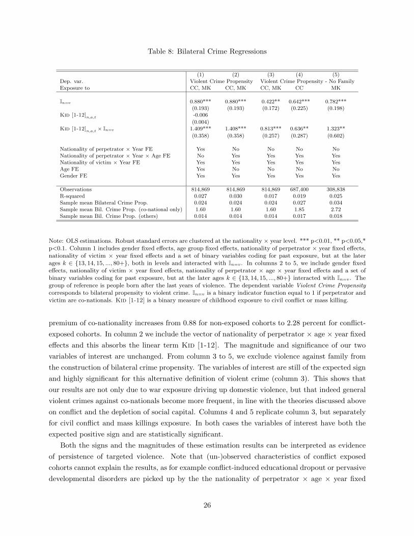
Table 8: Bilateral Crime Regressions

(1) (2) (3) (4) (5)Dep. var. Violent Crime Propensity Violent Crime Propensity - No FamilyExposure to CC, MK CC, MK CC, MK CC MK

In=v 0.880*** 0.880*** 0.422** 0.642*** 0.782***(0.193) (0.193) (0.172) (0.225) (0.198)

Kid [1-12]n,a,t -0.006

(0.004)Kid [1-12]n,a,t × In=v 1.409*** 1.408*** 0.813*** 0.636** 1.323**

(0.358) (0.358) (0.257) (0.287) (0.602)

Nationality of perpetrator × Year FE Yes No No No NoNationality of perpetrator × Year × Age FE No Yes Yes Yes YesNationality of victim × Year FE Yes Yes Yes Yes YesAge FE Yes No No No NoGender FE Yes Yes Yes Yes Yes

Observations 814,869 814,869 814,869 687,400 308,838R-squared 0.027 0.030 0.017 0.019 0.025Sample mean Bilateral Crime Prop. 0.024 0.024 0.024 0.027 0.034Sample mean Bil. Crime Prop. (co-national only) 1.60 1.60 1.60 1.85 2.72Sample mean Bil. Crime Prop. (others) 0.014 0.014 0.014 0.017 0.018

Note: OLS estimations. Robust standard errors are clustered at the nationality × year level. *** p<0.01, ** p<0.05,*p<0.1. Column 1 includes gender fixed effects, age group fixed effects, nationality of perpetrator × year fixed effects,nationality of victim × year fixed effects and a set of binary variables coding for past exposure, but at the laterages k ∈ {13, 14, 15, ..., 80+}, both in levels and interacted with In=v. In columns 2 to 5, we include gender fixedeffects, nationality of victim × year fixed effects, nationality of perpetrator × age × year fixed effects and a set ofbinary variables coding for past exposure, but at the later ages k ∈ {13, 14, 15, ..., 80+} interacted with In=v. Thegroup of reference is people born after the last years of violence. The dependent variable Violent Crime Propensitycorresponds to bilateral propensity to violent crime. In=v is a binary indicator function equal to 1 if perpetrator andvictim are co-nationals. Kid [1-12] is a binary measure of childhood exposure to civil conflict or mass killing.

premium of co-nationality increases from 0.88 for non-exposed cohorts to 2.28 percent for conflict-

exposed cohorts. In column 2 we include the vector of nationality of perpetrator × age × year fixed

effects and this absorbs the linear term Kid [1-12]. The magnitude and significance of our two

variables of interest are unchanged. From column 3 to 5, we exclude violence against family from

the construction of bilateral crime propensity. The variables of interest are still of the expected sign

and highly significant for this alternative definition of violent crime (column 3). This shows that

our results are not only due to war exposure driving up domestic violence, but that indeed general

violent crimes against co-nationals become more frequent, in line with the theories discussed above

on conflict and the depletion of social capital. Columns 4 and 5 replicate column 3, but separately

for civil conflict and mass killings exposure. In both cases the variables of interest have both the

expected positive sign and are statistically significant.

Both the signs and the magnitudes of these estimation results can be interpreted as evidence

of persistence of targeted violence. Note that (un-)observed characteristics of conflict exposed

cohorts cannot explain the results, as for example conflict-induced educational dropout or pervasive

developmental disorders are picked up by the the nationality of perpetrator × age × year fixed

26

effects. In contrast, theories stressing that past conflict damaged social ties between co-nationals

and that distrust and grievances acquired in early childhood persist over the lifetime are consistent

with our findings.

6 Combating the Legacy of Conflict: The Role of Policies

In this section we study how institutions in the host country modulate the impact of past exposure

to conflict on current criminality of asylum seekers. Our question of interest is whether the “right”

design of institutions and policies can partly or fully alleviate the risk of increased criminality for

exposed individuals. This question is of foremost policy relevance: Often anti-asylum political

movements and populist parties use fear of crime as a major argument against offering protection

to refugees. If the optimal integration policies are able to substantially curb the risk of crime driven

by past conflict exposure, arguments against open door policies and humanitarian help would be

under severe pressure.

As described above, the key players in the asylum process are the Swiss cantons. The de-

centralized, federalist constitution of Switzerland guarantees substantial autonomy to the cantons,

which results in large cross-canton heterogeneity of integration policies. Because asylum seekers are

early on allocated by the federal state to different cantons, their incentives for engaging in crime

or abiding the law are consequently shaped by the various local policies that cantons put in place.

Notice that due to the absence of a randomization scheme in the implementation of policies at the

canton-level, our exercise of policy evaluation can barely go beyond correlations. Though limited,

this preliminary evidence is, to our knowledge, new to the literature and fills a gap by documenting

how public policies can tackle the recurrence of violence in the aftermath of conflict.

The reference model of crime has been proposed by Becker (1968): the decision to commit a

crime is driven by the opportunity cost (legal labor market salaries) relative to returns to crime

discounted by the probability of being caught by the police and the sanction imposed by the criminal

justice system. Following a Beckerian logic of potential criminals trading off the gains and costs

of committing a crime, we now focus on cantonal policies that are likely to shape asylum seekers’

incentives. To this purpose we need to operate again with our cohort-level sample disaggregated at

the canton level (see Table 18). We now simply proceed by including in the disaggregated version

of equation (1) an interaction term between our main explanatory variable, Kid [1-12]n,a,t, and

various indicators of cantonal policies. The linear terms of the cantonal policies are absorbed by the

canton×year fixed effects. Like in Table 18, we include gender fixed effects, age group fixed effects,

canton × year fixed effects, nationality × year fixed effects and a set of binary variables coding for

past exposure, but at the later ages k ∈ {13, 14, 15, ..., 80+}. In addition, we also control for the

interaction of our set of indicators of cantonal policies with the set of binary variables coding for

past exposure at later ages k.

Tables 9 and 10 report the estimation results and Figures 4 and 5 in the Appendix display some

marginal effects. Note that for ease of interpretation, we normalize all continuous variables by their

27

average level. In all specifications standard errors are two-way clustered at the canton×year and

nationality×year levels. The definitions of all cantonal policies and control variables are relegated

to appendix E and summary statistics are displayed in Table 20.

Labor Market Integration– We start in Table 9 with policies related to the labor market

integration of asylum seekers. A main factor affecting the opportunity cost of engaging in criminal

activity is indeed the outside option of paid employment.20 This factor is particularly salient for

asylum seekers who are often severely cash constrained and many of which have indebted themselves

heavily to finance the travel to Europe.

In column 1 we interact conflict exposure with two mutually exclusive labor market features.

Open job accessc = 0 codes for cantons where asylum seekers are not allowed to rapidly search for

paid employment and where there are cantonal constraints and bans from paid work. In contrast,

Open job accessc = 1 corresponds to cantons where asylum seeker are allowed to rapidly search

for paid employment. The results show that in cantons without rapid labor market access past

exposure to conflict statistically significantly increases the crime propensity, while in cantons with

open job access there is no significant effect of exposure on crime propensity.

Not only the de jure job access is important, but also the help provided for getting integrated

in the job market. In column 2 we thus focus on the policy variable Promote job marketc that

takes a value of 1 for all cantons that offer active promotion services for labor market access, and

zero otherwise. The regression results stress that conflict exposure only boosts crime propensity

in the absence of active job promotion. Column 3 is dedicated to Professional trainingc that

codes for cantons offering at least one measure promoting professional training, such as coaching,

training, internships. Here also we find that past conflict exposure leads to an increase in crime

propensity only in cantons where professional training is not provided.

These first three columns contain measures that do not only correlate with actual employment

rates, but also affect behavior through encouragement and aspirations, even for those who have not

obtained an employment yet. Still, it is also interesting to consider more narrow variables capturing

very directly the de facto employment rates. Columns 4 and 5 report the results and Figure 4 dis-

plays the marginal effects. In column 4 war exposure is interacted with Occupation raten,c,t−1

at the level of the nationality-canton in the previous year. For example for Afghans in the canton

of Zurich in 2012 their occupation variable corresponds to the average occupation rate of Afghans

20This issue has received considerable attention in public debates and the press ( http://www.nytimes.com/2015/09/18/business/international/migrants-refugees-jobs-germany.html?_r=0, and http://www.economist.com/

news/leaders/21662547-bigger-welcome-mat-would-be-europes-own-interest-let-them-and-let-them-earn).Also the academic literature on crime has found that labor market access critically affects criminal behavior (seeDraca and Machin (2015) and Freeman (1999) for reviews of the literature). Fougere et al. (2009) for France andGould et al. (2002) for the US find a positive association between youth crime and youth unemployment, whileGould et al. (2002) show that the negative effect of earnings on crimes is stronger than the effect of employment.Further, Machin and Meghir (2004) use a wage measure for the low-skilled and find that an increase in this measurecorresponds to a fall in the crime rate. Bell et al. (2014) analyze the link between recessions and crimes and findthat young people who leave school in the midst of recessions are significantly more likely to become criminals thanthose who do not. Finally, Bell et al. (2013) find that asylum seeker inflows may have a positive effect on the crimerates in the UK, while economic migrant inflows (with arguably better labor market access) have no such effect.

28

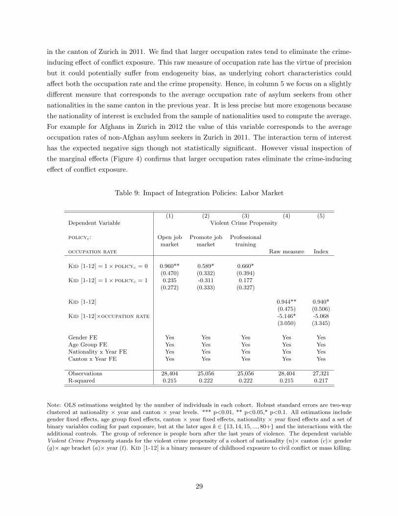
in the canton of Zurich in 2011. We find that larger occupation rates tend to eliminate the crime-

inducing effect of conflict exposure. This raw measure of occupation rate has the virtue of precision

but it could potentially suffer from endogeneity bias, as underlying cohort characteristics could

affect both the occupation rate and the crime propensity. Hence, in column 5 we focus on a slightly

different measure that corresponds to the average occupation rate of asylum seekers from other

nationalities in the same canton in the previous year. It is less precise but more exogenous because

the nationality of interest is excluded from the sample of nationalities used to compute the average.

For example for Afghans in Zurich in 2012 the value of this variable corresponds to the average

occupation rates of non-Afghan asylum seekers in Zurich in 2011. The interaction term of interest

has the expected negative sign though not statistically significant. However visual inspection of

the marginal effects (Figure 4) confirms that larger occupation rates eliminate the crime-inducing

effect of conflict exposure.

Table 9: Impact of Integration Policies: Labor Market

(1) (2) (3) (4) (5)Dependent Variable Violent Crime Propensity

policyc: Open job Promote job Professionalmarket market training

occupation rate Raw measure Index

Kid [1-12] = 1× policyc = 0 0.960** 0.589* 0.660*(0.470) (0.332) (0.394)

Kid [1-12] = 1× policyc = 1 0.235 -0.311 0.177(0.272) (0.333) (0.327)

Kid [1-12] 0.944** 0.940*(0.475) (0.506)

Kid [1-12]×occupation rate -5.146* -5.068(3.050) (3.345)

Gender FE Yes Yes Yes Yes YesAge Group FE Yes Yes Yes Yes YesNationality x Year FE Yes Yes Yes Yes YesCanton x Year FE Yes Yes Yes Yes Yes

Observations 28,404 25,056 25,056 28,404 27,321R-squared 0.215 0.222 0.222 0.215 0.217

Note: OLS estimations weighted by the number of individuals in each cohort. Robust standard errors are two-wayclustered at nationality × year and canton × year levels. *** p<0.01, ** p<0.05,* p<0.1. All estimations includegender fixed effects, age group fixed effects, canton × year fixed effects, nationality × year fixed effects and a set ofbinary variables coding for past exposure, but at the later ages k ∈ {13, 14, 15, ..., 80+} and the interactions with theadditional controls. The group of reference is people born after the last years of violence. The dependent variableViolent Crime Propensity stands for the violent crime propensity of a cohort of nationality (n)× canton (c)× gender(g)× age bracket (a)× year (t). Kid [1-12] is a binary measure of childhood exposure to civil conflict or mass killing.

29

Social Integration and Financial Support– Labor market integration is intertwined with social

integration, and one can expect social integration to reduce the crime risk directly by increasing the

opportunity cost of unlawful behavior, as well as indirectly by improving labor market outcomes.

We thus focus in Table 10 on measures of social integration and financial support.

In column 1 we interact conflict exposure with Civic and language coursesc that codes for

cantons where both language and civic education courses are offered. The rationale is that knowing

well the language and social norms of the host country is an important factor affecting the social

and economic integration. Strikingly, the crime inducing impact of conflict exposure is only present

in cantons that do not jointly offer language and civic education courses.

In column 2 we investigate how the method of management of asylum centers and level of

funding affect crime incentives. The variable Private managementc takes a value of 1 in cantons

where at least one cantonal or municipal asylum accommodation is run by a private firm, and zero

otherwise.21 One reason for cantons to outsource asylum services to private firms is to save on costs,

and in the Swiss media there has been a considerable controversy on whether quality standards

are guaranteed when private for-profit companies run asylum structures.22 The coefficient of the

interaction between Kid [1-12] and Private managementc = 1 is positive and significant, while

it is not significant for the interaction with Private managementc = 0, suggesting that private

asylum center management goes along with a higher crime propensity, while this is not the case for

non-private accommodation. Our data however do not allow us to identify whether this is due to

specific management principles applied by private firms (e.g. cutting costly integration programs

to maximize benefits), or whether this effect is rather due to a general willingness from the canton

side to cut costs.

We turn in column 3 to a more direct measure of financial support provided by public admin-

istrations to asylum seekers. The variable Social assistancec,t corresponds to the log of total

public money attributed per asylum seeker per month in a given canton c and year t. More financial

assistance and better funded asylum centers are expected to increase the opportunity cost of crime

by making less attractive the risk of being expelled from a better material situation in case of crime

conviction. Hence, we expect more financial assistance and better funded accommodation struc-

tures to deter crime. Surprisingly, neither the coefficient of the interaction term nor the marginal

effects (in Figure 5) are statistically significant.

Another important aspect of integration policies relates to the outcome of the demand for po-

litical asylum: Presumably asylum seekers with a serious chance of obtaining political asylum have

higher incentives to abide the law in order to maximize their asylum chances as compared to asylum

21The reason we are unable to code a continuous variable is that for several cantons we only know if private firmsoperate but the data on the number of asylum centers with and without private management is missing. Manycantons also have a huge diversity of types of accommodation, ranging from private flats to large centers. Computingsome average share of privately run centers in the absence of exhaustive information on their capacity could resultin substantial measurement error. For the few cantons with detailed information, the share of privately run centerswas either zero or very large, which suggest that working with a dummy variable is appropriate.

22See, for example, a recent article in the Swiss daily newspaper Tages-anzeiger, http://www.tagesanzeiger.ch/schweiz/standard/den-lohn-von-fluechtlingen-eingezogen/story/12513956.

30

seekers whose asylum demand has no chance. We consider the variable Acceptance raten,t that

corresponds to the percentage of recognized refugees (residence B permit) among asylum seeker

demands, by nationality n in year t: Its interaction term with war exposure in column 4 has the

expected negative sign, but is not statistically significant. Figure 5 displays the marginal effects.

Related to the outcome of the demand for political asylum is the existence, for a subset of

nationalities, of bilateral readmission agreements between Switzerland and the country of origin.

When an asylum seeker sees her application for refugee status rejected and is from a country with

a readmission agreement, Switzerland is able to send her back to her country of origin by force. In

contrast, people originating from countries without readmission agreement do not face this threat, as

Switzerland is not able to expel them by force even if their asylum application has been rejected. We

code a binary variable, Readmissionn, that is equal to 1 if there exists such a bilateral readmission

agreement for nationality n. Readmission agreements can be expected to have countervailing effects,

as on the one hand they increase the potential consequences of breaking the law and jeopardizing

the asylum application, while on the other hand they shorten the ex ante expected time horizon

in Switzerland, and hence the payoff of cooperation in a repeated setting. As far as the overall

effect is concerned, as shown in column 5, the coefficient of this variable has a positive sign, but

is not statistically significant. However, it is possible to disentangle the two countervailing forces.

Imagine someone with very low chances of being granted refugee status. In this case having a

readmission agreement shortens the time horizon in Switzerland and hence reduces the incentives

for cooperation. Thus it unambiguously increases the crime risk, and we should expect a positive

coefficient for readmission. Now consider someone with very high chances of obtaining refugee

status in Switzerland. When abiding the law, the person is likely to be able to stay in Switzerland

in the long-run, while when becoming criminal she may be expelled if a readmission agreement

exists. Hence, a readmission agreement in this case means that the price of being caught is higher,

and hence it lowers the crime incentives. One should in this case expect a negative coefficient

of readmission. To check this, we implement the triple interaction of conflict exposure with the

acceptance rate and readmission agreement variables. As shown in column 6, this triple interaction

term is negative and statistically significant, which suggests that readmission agreements drive up

crime incentives when acceptance chances are low, but that readmission agreements lower crime

when acceptance chances are high, exactly as predicted by the Beckerian logic outlined above.

7 Economic Migrants

For the purpose of causal identification our analysis has focused so far on asylum seekers because

this type of migrants are exogenously allocated across cantons. Nevertheless, it could be argued

that this population has peculiar (un)observed characteristics – in term of migration incentives and

background – and this could cast some doubt on the external validity of our analysis. To check

if our results apply to broader contexts as well, we replicate our baseline estimates focusing on

economic migrants.

31

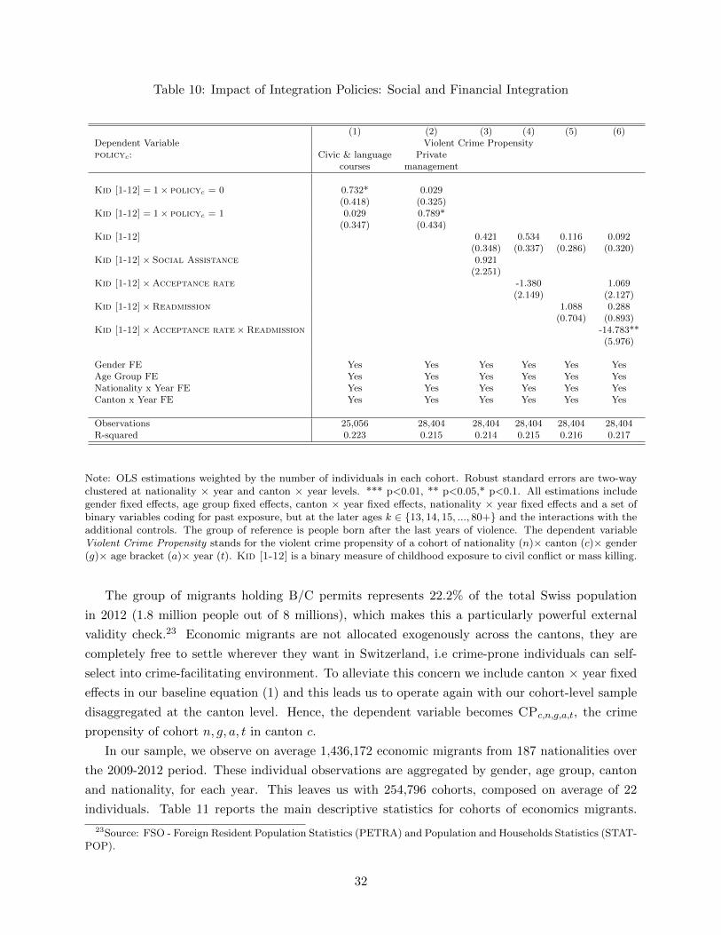
Table 10: Impact of Integration Policies: Social and Financial Integration

(1) (2) (3) (4) (5) (6)Dependent Variable Violent Crime Propensitypolicyc: Civic & language Private

courses management

Kid [1-12] = 1× policyc = 0 0.732* 0.029(0.418) (0.325)

Kid [1-12] = 1× policyc = 1 0.029 0.789*(0.347) (0.434)

Kid [1-12] 0.421 0.534 0.116 0.092(0.348) (0.337) (0.286) (0.320)

Kid [1-12]× Social Assistance 0.921(2.251)

Kid [1-12]×Acceptance rate -1.380 1.069(2.149) (2.127)

Kid [1-12]×Readmission 1.088 0.288(0.704) (0.893)

Kid [1-12]×Acceptance rate×Readmission -14.783**(5.976)

Gender FE Yes Yes Yes Yes Yes YesAge Group FE Yes Yes Yes Yes Yes YesNationality x Year FE Yes Yes Yes Yes Yes YesCanton x Year FE Yes Yes Yes Yes Yes Yes

Observations 25,056 28,404 28,404 28,404 28,404 28,404R-squared 0.223 0.215 0.214 0.215 0.216 0.217

Note: OLS estimations weighted by the number of individuals in each cohort. Robust standard errors are two-wayclustered at nationality × year and canton × year levels. *** p<0.01, ** p<0.05,* p<0.1. All estimations includegender fixed effects, age group fixed effects, canton × year fixed effects, nationality × year fixed effects and a set ofbinary variables coding for past exposure, but at the later ages k ∈ {13, 14, 15, ..., 80+} and the interactions with theadditional controls. The group of reference is people born after the last years of violence. The dependent variableViolent Crime Propensity stands for the violent crime propensity of a cohort of nationality (n)× canton (c)× gender(g)× age bracket (a)× year (t). Kid [1-12] is a binary measure of childhood exposure to civil conflict or mass killing.

The group of migrants holding B/C permits represents 22.2% of the total Swiss population

in 2012 (1.8 million people out of 8 millions), which makes this a particularly powerful external

validity check.23 Economic migrants are not allocated exogenously across the cantons, they are

completely free to settle wherever they want in Switzerland, i.e crime-prone individuals can self-

select into crime-facilitating environment. To alleviate this concern we include canton × year fixed

effects in our baseline equation (1) and this leads us to operate again with our cohort-level sample

disaggregated at the canton level. Hence, the dependent variable becomes CPc,n,g,a,t, the crime

propensity of cohort n, g, a, t in canton c.

In our sample, we observe on average 1,436,172 economic migrants from 187 nationalities over

the 2009-2012 period. These individual observations are aggregated by gender, age group, canton

and nationality, for each year. This leaves us with 254,796 cohorts, composed on average of 22

individuals. Table 11 reports the main descriptive statistics for cohorts of economics migrants.

23Source: FSO - Foreign Resident Population Statistics (PETRA) and Population and Households Statistics (STAT-POP).

32

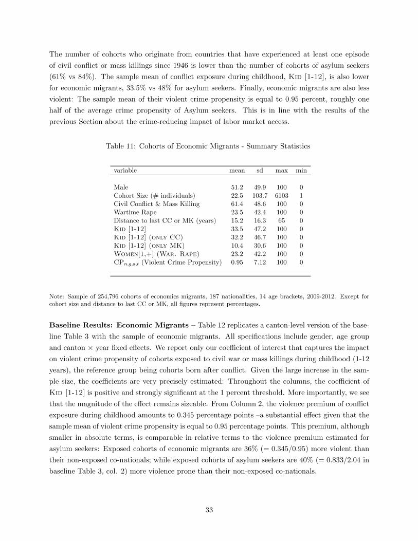
The number of cohorts who originate from countries that have experienced at least one episode

of civil conflict or mass killings since 1946 is lower than the number of cohorts of asylum seekers

(61% vs 84%). The sample mean of conflict exposure during childhood, Kid [1-12], is also lower

for economic migrants, 33.5% vs 48% for asylum seekers. Finally, economic migrants are also less

violent: The sample mean of their violent crime propensity is equal to 0.95 percent, roughly one

half of the average crime propensity of Asylum seekers. This is in line with the results of the

previous Section about the crime-reducing impact of labor market access.

Table 11: Cohorts of Economic Migrants - Summary Statistics

variable mean sd max min

Male 51.2 49.9 100 0Cohort Size (# individuals) 22.5 103.7 6103 1Civil Conflict & Mass Killing 61.4 48.6 100 0Wartime Rape 23.5 42.4 100 0Distance to last CC or MK (years) 15.2 16.3 65 0Kid [1-12] 33.5 47.2 100 0Kid [1-12] (only CC) 32.2 46.7 100 0Kid [1-12] (only MK) 10.4 30.6 100 0Women[1,+] (War. Rape) 23.2 42.2 100 0CPn,g,a,t (Violent Crime Propensity) 0.95 7.12 100 0

Note: Sample of 254,796 cohorts of economics migrants, 187 nationalities, 14 age brackets, 2009-2012. Except forcohort size and distance to last CC or MK, all figures represent percentages.

Baseline Results: Economic Migrants – Table 12 replicates a canton-level version of the base-

line Table 3 with the sample of economic migrants. All specifications include gender, age group

and canton × year fixed effects. We report only our coefficient of interest that captures the impact

on violent crime propensity of cohorts exposed to civil war or mass killings during childhood (1-12

years), the reference group being cohorts born after conflict. Given the large increase in the sam-

ple size, the coefficients are very precisely estimated: Throughout the columns, the coefficient of

Kid [1-12] is positive and strongly significant at the 1 percent threshold. More importantly, we see

that the magnitude of the effect remains sizeable. From Column 2, the violence premium of conflict

exposure during childhood amounts to 0.345 percentage points –a substantial effect given that the

sample mean of violent crime propensity is equal to 0.95 percentage points. This premium, although

smaller in absolute terms, is comparable in relative terms to the violence premium estimated for

asylum seekers: Exposed cohorts of economic migrants are 36% (= 0.345/0.95) more violent than

their non-exposed co-nationals; while exposed cohorts of asylum seekers are 40% (= 0.833/2.04 in

baseline Table 3, col. 2) more violence prone than their non-exposed co-nationals.

33

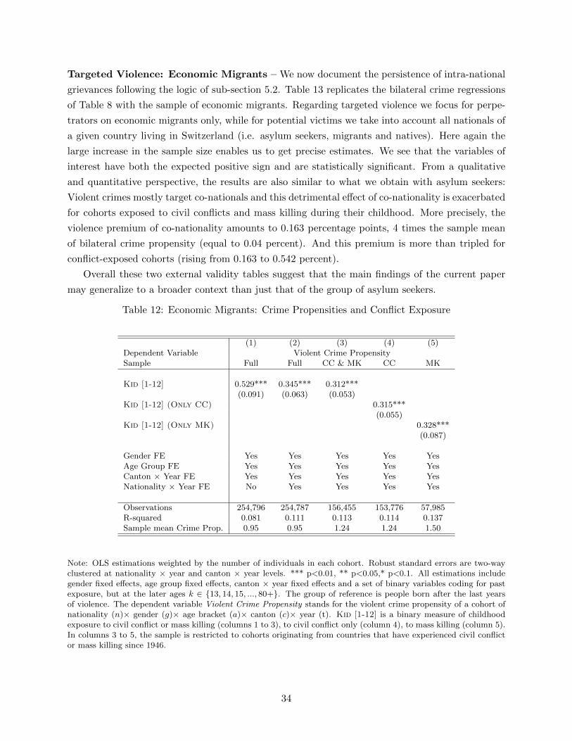
Targeted Violence: Economic Migrants – We now document the persistence of intra-national

grievances following the logic of sub-section 5.2. Table 13 replicates the bilateral crime regressions

of Table 8 with the sample of economic migrants. Regarding targeted violence we focus for perpe-

trators on economic migrants only, while for potential victims we take into account all nationals of

a given country living in Switzerland (i.e. asylum seekers, migrants and natives). Here again the

large increase in the sample size enables us to get precise estimates. We see that the variables of

interest have both the expected positive sign and are statistically significant. From a qualitative

and quantitative perspective, the results are also similar to what we obtain with asylum seekers:

Violent crimes mostly target co-nationals and this detrimental effect of co-nationality is exacerbated

for cohorts exposed to civil conflicts and mass killing during their childhood. More precisely, the

violence premium of co-nationality amounts to 0.163 percentage points, 4 times the sample mean

of bilateral crime propensity (equal to 0.04 percent). And this premium is more than tripled for

conflict-exposed cohorts (rising from 0.163 to 0.542 percent).

Overall these two external validity tables suggest that the main findings of the current paper

may generalize to a broader context than just that of the group of asylum seekers.

Table 12: Economic Migrants: Crime Propensities and Conflict Exposure

(1) (2) (3) (4) (5)Dependent Variable Violent Crime PropensitySample Full Full CC & MK CC MK

Kid [1-12] 0.529*** 0.345*** 0.312***(0.091) (0.063) (0.053)

Kid [1-12] (Only CC) 0.315***(0.055)

Kid [1-12] (Only MK) 0.328***(0.087)

Gender FE Yes Yes Yes Yes YesAge Group FE Yes Yes Yes Yes YesCanton × Year FE Yes Yes Yes Yes YesNationality × Year FE No Yes Yes Yes Yes

Observations 254,796 254,787 156,455 153,776 57,985R-squared 0.081 0.111 0.113 0.114 0.137Sample mean Crime Prop. 0.95 0.95 1.24 1.24 1.50

Note: OLS estimations weighted by the number of individuals in each cohort. Robust standard errors are two-wayclustered at nationality × year and canton × year levels. *** p<0.01, ** p<0.05,* p<0.1. All estimations includegender fixed effects, age group fixed effects, canton × year fixed effects and a set of binary variables coding for pastexposure, but at the later ages k ∈ {13, 14, 15, ..., 80+}. The group of reference is people born after the last yearsof violence. The dependent variable Violent Crime Propensity stands for the violent crime propensity of a cohort ofnationality (n)× gender (g)× age bracket (a)× canton (c)× year (t). Kid [1-12] is a binary measure of childhoodexposure to civil conflict or mass killing (columns 1 to 3), to civil conflict only (column 4), to mass killing (column 5).In columns 3 to 5, the sample is restricted to cohorts originating from countries that have experienced civil conflictor mass killing since 1946.

34

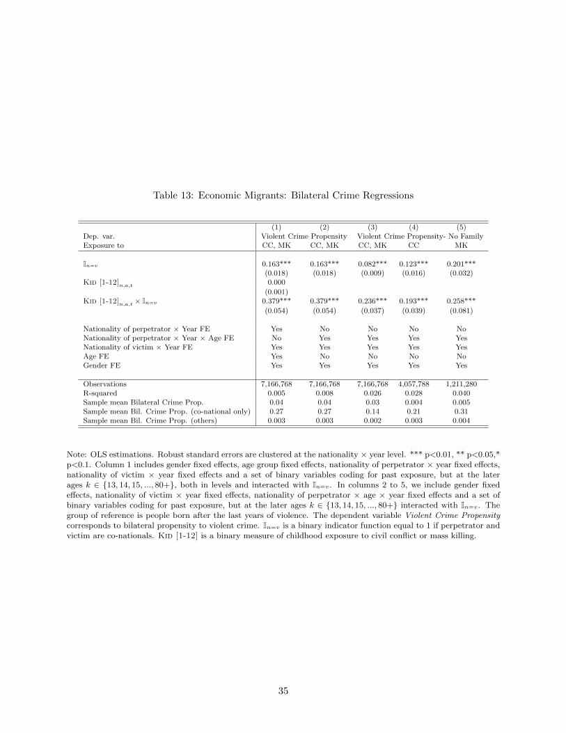
Table 13: Economic Migrants: Bilateral Crime Regressions

(1) (2) (3) (4) (5)Dep. var. Violent Crime Propensity Violent Crime Propensity- No FamilyExposure to CC, MK CC, MK CC, MK CC MK

In=v 0.163*** 0.163*** 0.082*** 0.123*** 0.201***(0.018) (0.018) (0.009) (0.016) (0.032)

Kid [1-12]n,a,t 0.000

(0.001)Kid [1-12]n,a,t × In=v 0.379*** 0.379*** 0.236*** 0.193*** 0.258***

(0.054) (0.054) (0.037) (0.039) (0.081)

Nationality of perpetrator × Year FE Yes No No No NoNationality of perpetrator × Year × Age FE No Yes Yes Yes YesNationality of victim × Year FE Yes Yes Yes Yes YesAge FE Yes No No No NoGender FE Yes Yes Yes Yes Yes

Observations 7,166,768 7,166,768 7,166,768 4,057,788 1,211,280R-squared 0.005 0.008 0.026 0.028 0.040Sample mean Bilateral Crime Prop. 0.04 0.04 0.03 0.004 0.005Sample mean Bil. Crime Prop. (co-national only) 0.27 0.27 0.14 0.21 0.31Sample mean Bil. Crime Prop. (others) 0.003 0.003 0.002 0.003 0.004

Note: OLS estimations. Robust standard errors are clustered at the nationality × year level. *** p<0.01, ** p<0.05,*p<0.1. Column 1 includes gender fixed effects, age group fixed effects, nationality of perpetrator × year fixed effects,nationality of victim × year fixed effects and a set of binary variables coding for past exposure, but at the laterages k ∈ {13, 14, 15, ..., 80+}, both in levels and interacted with In=v. In columns 2 to 5, we include gender fixedeffects, nationality of victim × year fixed effects, nationality of perpetrator × age × year fixed effects and a set ofbinary variables coding for past exposure, but at the later ages k ∈ {13, 14, 15, ..., 80+} interacted with In=v. Thegroup of reference is people born after the last years of violence. The dependent variable Violent Crime Propensitycorresponds to bilateral propensity to violent crime. In=v is a binary indicator function equal to 1 if perpetrator andvictim are co-nationals. Kid [1-12] is a binary measure of childhood exposure to civil conflict or mass killing.

35

8 Conclusion

This paper shows that exposure to civil conflict and mass killings during childhood (1-12 years)

has a robust, strong and persistent magnifying effect on the propensity to violent crime later in

life. The baseline causal analysis is conducted with the population of asylum seekers in Switzerland

over the 2009-2012 period but similar conclusions are reached when the analysis is extended to the

population of economic migrants. Contrary to previous case studies of post-conflict reconstruction,

our empirical strategy, by focusing on migrants, allows to show that this persistence in violence is

not due to persistently bad institutions in post-conflict states, but that it continues to hold even

when people live in an environment with fully functional institutions (Switzerland).

Do the results of the paper advocate a more restrictive immigration policy? Not by any means.

Still, the legitimate need for protection of refugees needs to be traded-off against the legitimate

demand for domestic security. Hence, while a generous asylum policy should in our view be main-

tained, our results suggest that it is equally crucial to accompany well those welcomed in the host

country. By installing a well-funded asylum system that offers rapid access to local labor markets

and provides future perspectives and opportunities for integration, the risk of an increase in crime

perpetrated by migrants with conflict background can be well contained.

Our findings may also have implications for post-conflict reconstruction. The result on the key

role of labor market integration to break vicious cycles of persistent violence may apply more gen-

erally (as recently investigated by Blattman and Ralston, 2015), and calls for a particularly strong

involvement and support from donor countries in the first crucial years following conflict. While for

example the Marshall Plan has surely made a key contribution to Germany’s ”Wirtschaftswunder”

post-1945 and paved its way to stable democracy, this lesson may have been forgotten in recent

time, as witnessed by the ill-fated precipitated withdrawal from post-Gaddafi Libya. More research

on the role of jobs and long-run perspectives for post-conflict reconstruction should be encouraged.

36

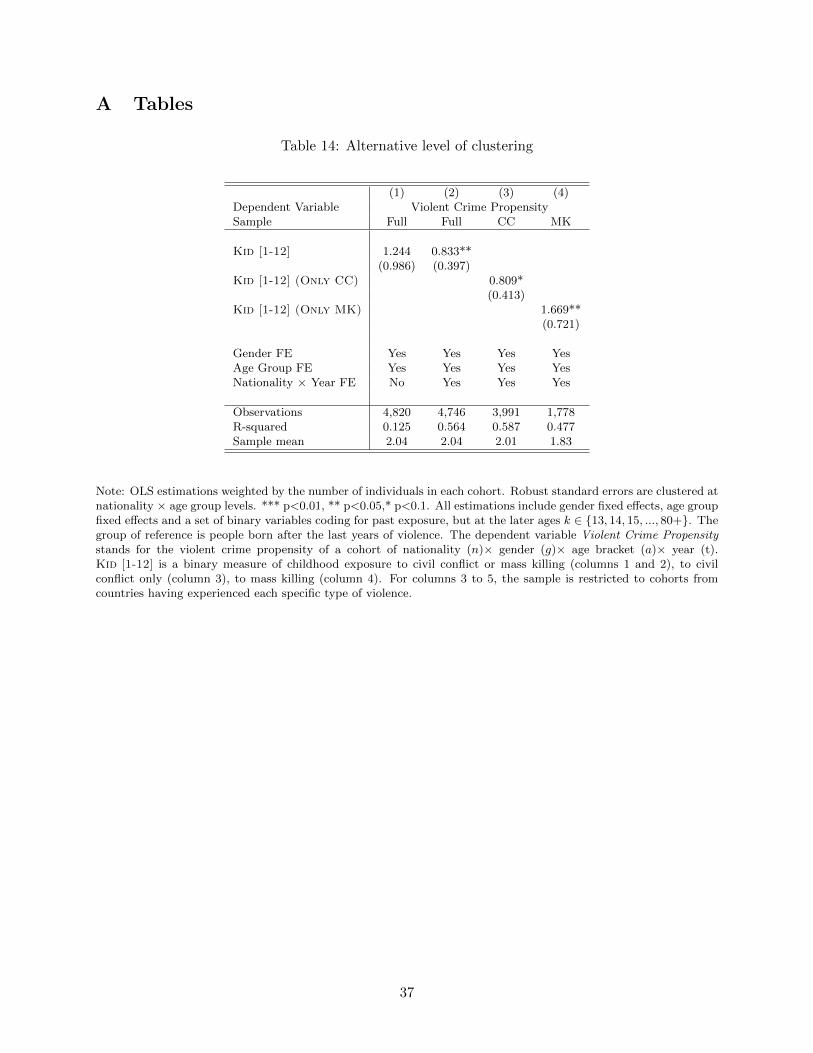
A Tables

Table 14: Alternative level of clustering

(1) (2) (3) (4)Dependent Variable Violent Crime PropensitySample Full Full CC MK

Kid [1-12] 1.244 0.833**(0.986) (0.397)

Kid [1-12] (Only CC) 0.809*(0.413)

Kid [1-12] (Only MK) 1.669**(0.721)

Gender FE Yes Yes Yes YesAge Group FE Yes Yes Yes YesNationality × Year FE No Yes Yes Yes

Observations 4,820 4,746 3,991 1,778R-squared 0.125 0.564 0.587 0.477Sample mean 2.04 2.04 2.01 1.83

Note: OLS estimations weighted by the number of individuals in each cohort. Robust standard errors are clustered atnationality × age group levels. *** p<0.01, ** p<0.05,* p<0.1. All estimations include gender fixed effects, age groupfixed effects and a set of binary variables coding for past exposure, but at the later ages k ∈ {13, 14, 15, ..., 80+}. Thegroup of reference is people born after the last years of violence. The dependent variable Violent Crime Propensitystands for the violent crime propensity of a cohort of nationality (n)× gender (g)× age bracket (a)× year (t).Kid [1-12] is a binary measure of childhood exposure to civil conflict or mass killing (columns 1 and 2), to civilconflict only (column 3), to mass killing (column 4). For columns 3 to 5, the sample is restricted to cohorts fromcountries having experienced each specific type of violence.

37

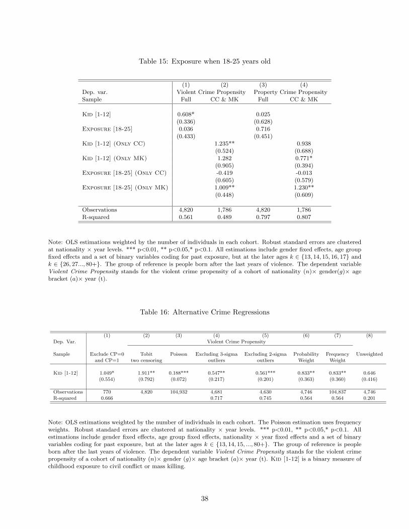
Table 15: Exposure when 18-25 years old

(1) (2) (3) (4)Dep. var. Violent Crime Propensity Property Crime PropensitySample Full CC & MK Full CC & MK

Kid [1-12] 0.608* 0.025(0.336) (0.628)

Exposure [18-25] 0.036 0.716(0.433) (0.451)

Kid [1-12] (Only CC) 1.235** 0.938(0.524) (0.688)

Kid [1-12] (Only MK) 1.282 0.771*(0.905) (0.394)

Exposure [18-25] (Only CC) -0.419 -0.013(0.605) (0.579)

Exposure [18-25] (Only MK) 1.009** 1.230**(0.448) (0.609)

Observations 4,820 1,786 4,820 1,786R-squared 0.561 0.489 0.797 0.807

Note: OLS estimations weighted by the number of individuals in each cohort. Robust standard errors are clusteredat nationality × year levels. *** p<0.01, ** p<0.05,* p<0.1. All estimations include gender fixed effects, age groupfixed effects and a set of binary variables coding for past exposure, but at the later ages k ∈ {13, 14, 15, 16, 17} andk ∈ {26, 27..., 80+}. The group of reference is people born after the last years of violence. The dependent variableViolent Crime Propensity stands for the violent crime propensity of a cohort of nationality (n)× gender(g)× agebracket (a)× year (t).

Table 16: Alternative Crime Regressions

(1) (2) (3) (4) (5) (6) (7) (8)Dep. Var. Violent Crime Propensity

Sample Exclude CP=0 Tobit Poisson Excluding 3-sigma Excluding 2-sigma Probability Frequency Unweightedand CP=1 two censoring outliers outliers Weight Weight

Kid [1-12] 1.049* 1.911** 0.188*** 0.547** 0.561*** 0.833** 0.833** 0.646(0.554) (0.792) (0.072) (0.217) (0.201) (0.363) (0.360) (0.416)

Observations 770 4,820 104,932 4,681 4,630 4,746 104,837 4,746R-squared 0.666 0.717 0.745 0.564 0.564 0.201

Note: OLS estimations weighted by the number of individuals in each cohort. The Poisson estimation uses frequencyweights. Robust standard errors are clustered at nationality × year levels. *** p<0.01, ** p<0.05,* p<0.1. Allestimations include gender fixed effects, age group fixed effects, nationality × year fixed effects and a set of binaryvariables coding for past exposure, but at the later ages k ∈ {13, 14, 15, ..., 80+}. The group of reference is peopleborn after the last years of violence. The dependent variable Violent Crime Propensity stands for the violent crimepropensity of a cohort of nationality (n)× gender (g)× age bracket (a)× year (t). Kid [1-12] is a binary measure ofchildhood exposure to civil conflict or mass killing.

38

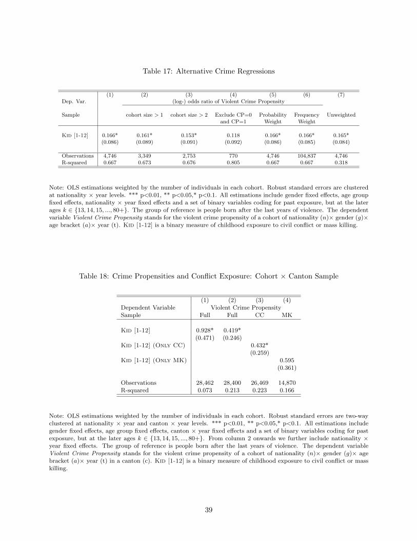
Table 17: Alternative Crime Regressions

(1) (2) (3) (4) (5) (6) (7)Dep. Var. (log-) odds ratio of Violent Crime Propensity

Sample cohort size > 1 cohort size > 2 Exclude CP=0 Probability Frequency Unweightedand CP=1 Weight Weight

Kid [1-12] 0.166* 0.161* 0.153* 0.118 0.166* 0.166* 0.165*(0.086) (0.089) (0.091) (0.092) (0.086) (0.085) (0.084)

Observations 4,746 3,349 2,753 770 4,746 104,837 4,746R-squared 0.667 0.673 0.676 0.805 0.667 0.667 0.318

Note: OLS estimations weighted by the number of individuals in each cohort. Robust standard errors are clusteredat nationality × year levels. *** p<0.01, ** p<0.05,* p<0.1. All estimations include gender fixed effects, age groupfixed effects, nationality × year fixed effects and a set of binary variables coding for past exposure, but at the laterages k ∈ {13, 14, 15, ..., 80+}. The group of reference is people born after the last years of violence. The dependentvariable Violent Crime Propensity stands for the violent crime propensity of a cohort of nationality (n)× gender (g)×age bracket (a)× year (t). Kid [1-12] is a binary measure of childhood exposure to civil conflict or mass killing.

Table 18: Crime Propensities and Conflict Exposure: Cohort × Canton Sample

(1) (2) (3) (4)Dependent Variable Violent Crime PropensitySample Full Full CC MK

Kid [1-12] 0.928* 0.419*(0.471) (0.246)

Kid [1-12] (Only CC) 0.432*(0.259)

Kid [1-12] (Only MK) 0.595(0.361)

Observations 28,462 28,400 26,469 14,870R-squared 0.073 0.213 0.223 0.166

Note: OLS estimations weighted by the number of individuals in each cohort. Robust standard errors are two-wayclustered at nationality × year and canton × year levels. *** p<0.01, ** p<0.05,* p<0.1. All estimations includegender fixed effects, age group fixed effects, canton × year fixed effects and a set of binary variables coding for pastexposure, but at the later ages k ∈ {13, 14, 15, ..., 80+}. From column 2 onwards we further include nationality ×year fixed effects. The group of reference is people born after the last years of violence. The dependent variableViolent Crime Propensity stands for the violent crime propensity of a cohort of nationality (n)× gender (g)× agebracket (a)× year (t) in a canton (c). Kid [1-12] is a binary measure of childhood exposure to civil conflict or masskilling.

39

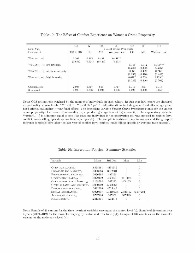
Table 19: The Effect of Conflict Experience on Women’s Crime Propensity

(1) (2) (3) (4) (5) (6) (7)Dep. Var. Violent Crime PropensityExposure to CC & MK CC MK Wartime rape CC MK Wartime rape

Women[1,+] 0.307 0.415 0.487 0.488**(0.654) (0.674) (0.425) (0.233)

Women[1,+] : low intensity 0.345 -0.312 0.755***(0.285) (0.332) (0.232)

Women[1,+] : medium intensity -0.071 0.489 0.744*(0.295) (0.416) (0.442)

Women[1,+] : high intensity 0.629* 0.739 1.739**(0.325) (0.446) (0.701)

Observations 2,008 1,717 843 1,717 1,717 843 1,717R-squared 0.290 0.286 0.294 0.256 0.292 0.300 0.257

Note: OLS estimations weighted by the number of individuals in each cohort. Robust standard errors are clusteredat nationality × year levels. *** p<0.01, ** p<0.05,* p<0.1. All estimations include gender fixed effects, age groupfixed effects, nationality × year fixed effects. The dependent variable Violent Crime Propensity stands for the violentcrime propensity of a cohort of nationality (n)× gender (g)× age bracket (a)× year (t). The explanatory variable,Women[1,+] is a dummy equal to one if at least one individual in the observation cell was exposed to conflict (civilconflict, mass killing episode or wartime rape episode). The sample is restricted only to women and the group ofreference is people born after the last year of conflict (civil conflict, mass killing episode or wartime rape episode).

Table 20: Integration Policies - Summary Statistics

Variable Mean Std.Dev. Max Min

Open job accessc .6538461 .4851645 1 0Promote job marketc .1363636 .3512501 1 0Professional trainingc .3636364 .492366 1 0Occupation ratenct .1022142 .063855 .3513073 0Occupation rate: Indexnct .1128592 .067392 .406135 0Civic & language coursesc .4090909 .5032363 1 0Private managementc .2692308 .4523443 1 0Social assistancect 6.929337 0.1319578 7.324757 6.607203Acceptance raten .0767988 .105302 .537329 0Readmissionn .2313311 .4232513 1 0

Note: Sample of 26 cantons for the time-invariant variables varying at the canton level (c). Sample of 26 cantons over4 years (2009-2012) for the variables varying by canton and over time (c,t). Sample of 134 countries for the variablesvarying at the nationality level (n).

40

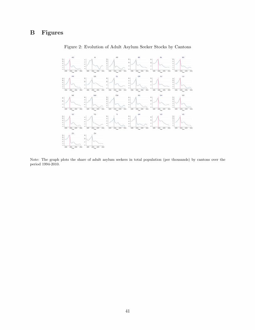
B Figures

Figure 2: Evolution of Adult Asylum Seeker Stocks by Cantons

24

68

1012

1995 2000 2005 2010Year

AG

23

45

6

1995 2000 2005 2010Year

AI

24

68

1012

1995 2000 2005 2010Year

AR

05

1015

1995 2000 2005 2010Year

BE

05

1015

1995 2000 2005 2010Year

BL

02

46

810

1995 2000 2005 2010Year

BS

24

68

1012

1995 2000 2005 2010Year

FR

05

1015

1995 2000 2005 2010Year

GE

05

1015

1995 2000 2005 2010Year

GL

24

68

10

1995 2000 2005 2010Year

GR

05

1015

1995 2000 2005 2010Year

JU

24

68

1012

1995 2000 2005 2010Year

LU

05

1015

1995 2000 2005 2010Year

NE

24

68

10

1995 2000 2005 2010Year

NW

24

68

1012

1995 2000 2005 2010Year

OW

24

68

10

1995 2000 2005 2010Year

SG

05

1015

1995 2000 2005 2010Year

SH

24

68

1012

1995 2000 2005 2010Year

SO

24

68

1012

1995 2000 2005 2010Year

SZ

02

46

8

1995 2000 2005 2010Year

TG

24

68

10

1995 2000 2005 2010Year

TI

24

68

101995 2000 2005 2010

Year

UR

05

1015

1995 2000 2005 2010Year

VD

24

68

1012

1995 2000 2005 2010Year

VS

24

68

1012

1995 2000 2005 2010Year

ZG

05

1015

1995 2000 2005 2010Year

ZH

Note: The graph plots the share of adult asylum seekers in total population (per thousands) by cantons over theperiod 1994-2010.

41

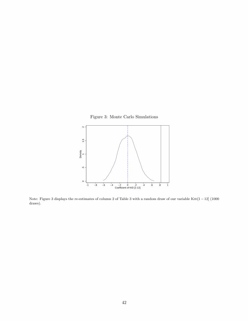
Figure 3: Monte Carlo Simulations

0.5

11.

52

Den

sity

-1 -.8 -.6 -.4 -.2 0 .2 .4 .6 .8 1Coefficient of KID [1-12]

Note: Figure 3 displays the re-estimates of column 2 of Table 3 with a random draw of our variable Kid[1−12] (1000draws).

42

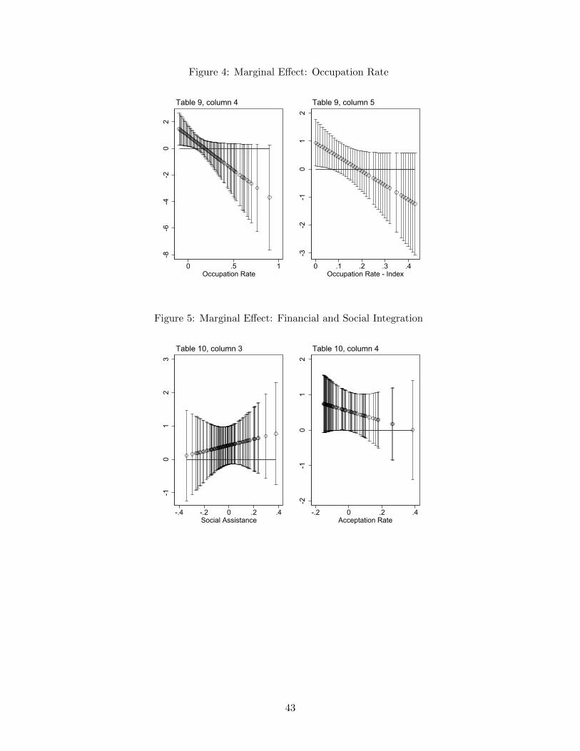
Figure 4: Marginal Effect: Occupation Rate

-8-6

-4-2

02

0 .5 1Occupation Rate

Table 9, column 4

-3-2

-10

12

0 .1 .2 .3 .4Occupation Rate - Index

Table 9, column 5

Figure 5: Marginal Effect: Financial and Social Integration

-10

12

3

-.4 -.2 0 .2 .4Social Assistance

Table 10, column 3

-2-1

01

2

-.2 0 .2 .4Acceptation Rate

Table 10, column 4

43

C Appendix on Political Asylum in Switzerland

C.1 The Demand for Asylum in Switzerland

Switzerland is a federal state with 26 cantons (i.e. the main sub-national entities) and a population

of about 8 million people. This country has a strong humanitarian tradition (starting in the 16th

century with providing large-scale refuge to the Huguenots fleeing France) and has traditionally

hosted many foreigners. While according to the Swiss Federal Statistical Office in 2012 about

23.3% of the population are foreign nationals, the number of asylum seekers –which are defined as

individuals who have applied and are waiting for being approved the refugee status– is considerably

smaller. In particular, in our data in 2012 there were slightly above 32’000 asylum seekers (with

the N permit), corresponding to about 0.4% of the Swiss population. The biggest cohorts for

our sample period came from Eritrea, Sri Lanka, Nigeria, Afghanistan, Somalia, Tunisia, Serbia,

Turkey, Iraq and Syria (see Table 1).

According to the United Nations Convention Relating to the Status of Refugees adopted in

1951 and signed by Switzerland, a refugee is a person who ”owing to well-founded fear of being

persecuted for reasons of race, religion, nationality, membership of a particular social group or

political opinion, is outside the country of his nationality and is unable or, owing to such fear, is

unwilling to avail himself of the protection of that country; or who, not having a nationality and

being outside the country of his former habitual residence as a result of such events, is unable

or, owing to such fear, is unwilling to return to it” (Article 1, A2). Thus, while of course many

migrants are motivated by the (legitimate) goal of escaping extreme poverty, to obtain refugee

status a person needs to be able to demonstrate persecution for political reasons.

C.2 The Procedure of Assessing Asylum Requests

Most asylum seekers enter Switzerland illegally (especially crossing the Italian border) and apply

for asylum in one of the four national reception and procedure centers (RPC) 24. Only few arrive

by plane in one of the two airport centers (Geneva and Zurich) or through asylum applications filed

at Swiss embassies abroad.25

In the RPC, asylum seekers go through a first interview, where they are asked to provide identity

proofs, fingerprints, and their application reasons. If there persist doubts about the identity and the

application reasons, language tests or lie detection techniques are used. After on average 100-120

days since the demand was made in the RPC 26, authorities declare ”non-credible” (“non-entree en

matiere” - NEM) around 50% of the 20000-25000 yearly treated demands, according to the Federal

Office of Migrations Statistics (2009-2012). Typical examples of demands judged ”non-credible”

are from nationals who either originate from safe countries, or who do not collaborate with the

24There are four reception centers close to the Swiss borders: Basel, Chiasso, Kreuzlingen, and Vallorbe.25On 28 September 2012, the Swiss Parliament abolished the possibility of applying for asylum from abroad.

However, the possibility to file a visa request with a Swiss diplomatic representation is still open.26The asylum process duration measures follow the estimations for 2008-2010 published in Rapport sur des mesures

d’acceleration dans le domaine d’asile, Departement federal de justice et police (2011).

44

authorities, who apply for asylum a second time after having already been rejected earlier or whose

demand has to be treated by another state according to the Dublin Agreement 27. When a demand

is judged ”non-credible” and, thus, rejected, the asylum seeker either voluntary leaves the country

or is detained and expelled by force (when possible).

The other half of asylum seekers whose demands are judged credible receive the N permit 28

(i.e. a temporary ”green card” for being allowed to stay in Switzerland during the duration of the

in-depth assessment of their asylum request). Given that assessing the threat of persecution in the

home country is hard, the asylum process naturally takes substantial time. Between 2008-2010,

the average duration of the process for credible asylum seekers (from the moment the demand was

made in one of the RPC until the first decision), was 300-400 days, with complex cases taking

several years.

Crucially, during this period holders of the N-permit are exogenously allocated to cantons and

are not allowed to change canton. The allocation of new N-permit holders to the 26 Swiss cantons

are determined precisely by a random allocation key based on the cantonal population. This

exogenous and random allocation of N-permit holders is crucial for the identification strategy of

our current paper, as it rules out self-selection of particular types of asylum seekers to particular

cantonal environments. Once an asylum seeker has been allocated to a given canton, the canton in

charge organizes the accommodation in cantonal centers or flats and takes care of the interviews

and of financial matters.29.

The accommodation procedure for asylum seekers takes place in two steps within the canton.

(Efionayi-Mader, 2011). In a first step, they are hosted in collective centers where their basic

needs are taken care of. In a second step, they are offered either private apartments or collective

accommodation in special centers. In about half of the cantons, families with children are offered

private accommodation. The diversity of accommodation possibilities across cantons is explained

by the housing availabilities, size of the canton, responsible organizations etc. We acknowledge

that while the exogenous allocation holds across cantons it may not hold inside cantons due to

housing availabilities. In other words, collective accommodation centers may sometimes be placed

in remote neighborhoods.

27The Dublin Association Agreement of 2008 between Switzerland and the EU ensures that a request for asylumsubmitted by an asylum-seeker is only examined by one state within the Schengen/Dublin Area (which includes mostEU member states in continental Europe, plus Switzerland, Norway and Iceland). The Dublin criteria establish whichcountry is responsible for dealing with a given asylum application, and aims to prevent asylum seekers from beingreferred from one country to another. If the asylum demand was rejected by this responsible state, then the asylumseeker cannot apply for asylum in another member state.

28In the individual crimes database, asylum seekers are reported with N-permit and non-credible asylum seekersare reported with NE. We only consider those with N-permit, thus the more credible ones. It might still be possiblethat non-credible asylum seekers are allocated to cantons if the decision takes more than 90 days.

29Cantons decide on the funds offered for social assistance and the Confederation supplies the funds needed.According to Efionayi-Mader (2011), the Confederation allocated, on average, 55,64 CHF per day per asylum seeker.

45

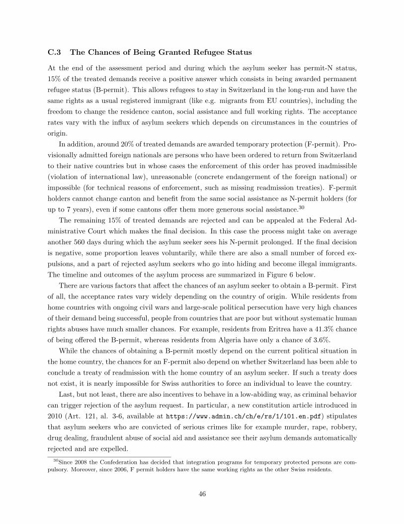
C.3 The Chances of Being Granted Refugee Status

At the end of the assessment period and during which the asylum seeker has permit-N status,

15% of the treated demands receive a positive answer which consists in being awarded permanent

refugee status (B-permit). This allows refugees to stay in Switzerland in the long-run and have the

same rights as a usual registered immigrant (like e.g. migrants from EU countries), including the

freedom to change the residence canton, social assistance and full working rights. The acceptance

rates vary with the influx of asylum seekers which depends on circumstances in the countries of

origin.

In addition, around 20% of treated demands are awarded temporary protection (F-permit). Pro-

visionally admitted foreign nationals are persons who have been ordered to return from Switzerland

to their native countries but in whose cases the enforcement of this order has proved inadmissible

(violation of international law), unreasonable (concrete endangerment of the foreign national) or

impossible (for technical reasons of enforcement, such as missing readmission treaties). F-permit

holders cannot change canton and benefit from the same social assistance as N-permit holders (for

up to 7 years), even if some cantons offer them more generous social assistance.30

The remaining 15% of treated demands are rejected and can be appealed at the Federal Ad-

ministrative Court which makes the final decision. In this case the process might take on average

another 560 days during which the asylum seeker sees his N-permit prolonged. If the final decision

is negative, some proportion leaves voluntarily, while there are also a small number of forced ex-

pulsions, and a part of rejected asylum seekers who go into hiding and become illegal immigrants.

The timeline and outcomes of the asylum process are summarized in Figure 6 below.

There are various factors that affect the chances of an asylum seeker to obtain a B-permit. First

of all, the acceptance rates vary widely depending on the country of origin. While residents from

home countries with ongoing civil wars and large-scale political persecution have very high chances

of their demand being successful, people from countries that are poor but without systematic human

rights abuses have much smaller chances. For example, residents from Eritrea have a 41.3% chance

of being offered the B-permit, whereas residents from Algeria have only a chance of 3.6%.

While the chances of obtaining a B-permit mostly depend on the current political situation in

the home country, the chances for an F-permit also depend on whether Switzerland has been able to

conclude a treaty of readmission with the home country of an asylum seeker. If such a treaty does

not exist, it is nearly impossible for Swiss authorities to force an individual to leave the country.

Last, but not least, there are also incentives to behave in a low-abiding way, as criminal behavior

can trigger rejection of the asylum request. In particular, a new constitution article introduced in

2010 (Art. 121, al. 3-6, available at https://www.admin.ch/ch/e/rs/1/101.en.pdf) stipulates

that asylum seekers who are convicted of serious crimes like for example murder, rape, robbery,

drug dealing, fraudulent abuse of social aid and assistance see their asylum demands automatically

rejected and are expelled.

30Since 2008 the Confederation has decided that integration programs for temporary protected persons are com-pulsory. Moreover, since 2006, F permit holders have the same working rights as the other Swiss residents.

46

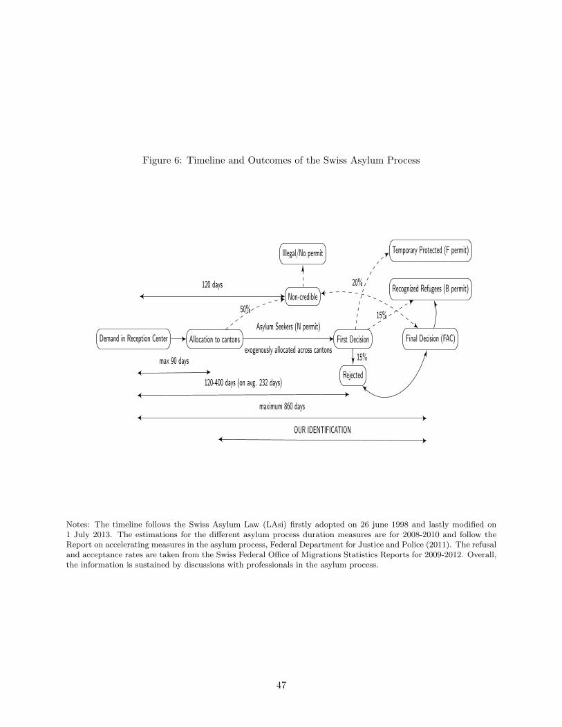
Figure 6: Timeline and Outcomes of the Swiss Asylum Process

Demand in Reception Center Allocation to cantons

max 90 days

First Decision

Asylum Seekers (N permit)

exogenously allocated across cantons

120-400 days (on avg. 232 days)

Final Decision (FAC)

Recognized Refugees (B permit)

Temporary Protected (F permit)

Non-credible

Illegal/No permit

Rejected

15%

20%

15%

50%

120 days

maximum 860 days

OUR IDENTIFICATION

Notes: The timeline follows the Swiss Asylum Law (LAsi) firstly adopted on 26 june 1998 and lastly modified on1 July 2013. The estimations for the different asylum process duration measures are for 2008-2010 and follow theReport on accelerating measures in the asylum process, Federal Department for Justice and Police (2011). The refusaland acceptance rates are taken from the Swiss Federal Office of Migrations Statistics Reports for 2009-2012. Overall,the information is sustained by discussions with professionals in the asylum process.

47

Successful integration efforts can also be rewarded through another channel. In special cases

(such as an asylum procedure lasting longer than 5 years or for several personal hardship reasons),

cantonal authorities can grant a residence (B) permit to asylum seekers under the condition of good

integration into the Swiss society31. The most important integration criteria refers to the respect

of laws: no police record, and no acts of default of goods and prosecution. The second important

criteria is the proof of financial independence (no need for social assistance). First, such a special

hardship demand needs to be accepted by the canton and then it has to be approved at the federal

level. While the cantonal decision cannot usually be repealed, the federal decision can be repealed.

31According to the Ordinance for the Integration of Foreigners (2008), integration criteria are defined as follows:respect of federal values, public order and security, willingness to have an economic activity and acquire training,knowledge of at least one Swiss language and Swiss living style. Duration of stay, family and health conditions, andthe possibility of reintegration into the country of origin are also taken into account.

48

D Formal test of the process of allocation

We now provide more formal statistical tests for the exogenous spatial allocation of asylum seekers

across cantons. The purpose of this is to tackle the question of whether there is indeed an exogenous

allocation of asylum seekers following the official population-based distribution key –as we claim–

or if there may be some selection on relevant dimensions. For example, such selective allocation

would occur if, say, the urban (supposedly more crime-prone) cantons of Zurich or Geneva were

more likely to host young males fleeing a conflict zone while rural and quiet cantons were to host

other asylum seekers.

In Table 21 we display a first approach where, for various observable cohort characteristics, we

test for the difference in means between cantons. To this purpose we consider a more fine-grained

version of our sample where, in year t, each cohort of nationality n, gender g, and age group a is

splitted across cantons c. In Column (1) we regress, for each nationality taken separately, each

observable on a battery of canton fixed effects. In case of endogenous spatial sorting in some

specific cantons, the fixed effects associated with those cantons should be statistically significantly

correlated with the cohort characteristics, and the F-test should be rejected for this nationality.

The reported figure corresponds to the share of nationalities for which the F-test is not rejected

at the 5 percent level. The first observable that we consider corresponds to our main explanatory

variable, e.g. the exposure to violence during childhood. We see that in 82% of cases our test does

not detect any endogenous spatial sorting based on this observable. Results are similar for the

alternative measures of exposure or for other first order determinants of crime, namely gender and

age (by brackets).

Our above approach to testing exogenous spatial allocation has the advantage of simplicity but

might not be ideally suited to our empirical context where the spatial units under consideration are

small. Indeed, the median nationality is composed of only 42 asylum seekers –sample average being

765– that have to be allocated across 26 cantons. In this type of context, as firstly pointed out

by Ellison and Glaeser (1997), a parametric test of spatial allocation/concentration (that assumes

independent location choices) might be ill-defined to test the null hypothesis of exogenous allocation.

Indeed, in presence of an exogenous allocation process that does not take into account the past

exposure to violence of asylum seekers, we should find a uniform distribution of past exposure

across the cantons only asymptotically, i.e. only if the size of each nationality is large enough.

Otherwise, for small nationality sizes, sampling variations will lead to observed patterns of spatial

concentration in some cantons.

Column (2) of Table 21 is a first attempt to tackle this sampling issue. The idea is to pool

cohorts from all nationalities by year before performing the F-test. The pool of asylum seekers

to be allocated is now much larger (on average 24,864 individuals per year) and this makes our

F-test more likely to meet the asymptotic requirement. For each observable, the reported statistic

corresponds to the number of years (out of 4) for which the F-test is not rejected. As expected,

the F-test performs now better.

In Column (3) we propose an alternative approach to circumvent the sampling issue in the test

49

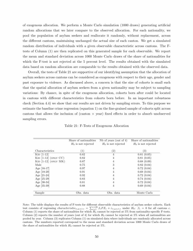
of exogenous allocation. We perform a Monte Carlo simulation (1000 draws) generating artificial

random allocations that we later compare to the observed allocation. For each nationality, we

pool the population of asylum seekers and reallocate it randomly, without replacement, across

the different cantons, maintaining unchanged the actual size of each canton. We get a simulated

random distribution of individuals with a given observable characteristic across cantons. The F-

tests of Column (1) are then replicated on this generated sample for each observable. We report

the mean and standard deviation across 1000 Monte Carlo draws of the share of nationalities for

which the F-test is not rejected at the 5 percent level. The results obtained with the simulated

data based on random allocation are comparable to the results obtained with the observed data.

Overall, the tests of Table 21 are supportive of our identifying assumption that the allocation of

asylum seekers across cantons can be considered as exogenous with respect to their age, gender and

past exposure to violence. As discussed above, a concern is that the size of cohorts is small such

that the spatial allocation of asylum seekers from a given nationality may be subject to sampling

variations: By chance, in spite of the exogenous allocation, cohorts born after could be located

in cantons with different characteristics from cohorts born before. In an important robustness

check (Section 4.4) we show that our results are not driven by sampling errors. To this purpose we

estimate the baseline crime regression (equation 1) on the fine-grained sample of cohorts split across

cantons that allows the inclusion of (canton × year) fixed effects in order to absorb unobserved

sampling errors.

Table 21: F-Tests of Exogenous Allocation

Share of nationalities Nb of years (out of 4) Share of nationalitiesH0 is not rejected H0 is not rejected H0 is not rejected

Characteristics (1) (2) (3)

Kid [1-12] 0.82 4 0.81 (0.05)Kid [1-12] (only CC) 0.82 4 0.81 (0.05)Kid [1-12] (only MK) 0.87 4 0.68 (0.09)Male 0.75 3 0.82 (0.04)Age [16-17] 0.97 4 0.72 (0.04)Age [18-20] 0.91 4 0.69 (0.04)Age [21-24] 0.92 4 0.72 (0.04)Age [25-29] 0.83 4 0.74 (0.04)Age [30-34] 0.81 4 0.72 (0.04)Age [35-39] 0.88 4 0.69 (0.04)

Sample Obs. data Obs. data Monte Carlo

Note: The table displays the results of F-tests for different observable characteristics of asylum seeker cohorts. Eachtest consists of regressing characteristicn,g,a,t,c =

∑c=26c=1 βcFEc + εn,g,a,t,c under H0: βc = 0 for all cantons c.

Column (1) reports the share of nationalities for which H0 cannot be rejected at 5% from nationality-specific F-tests.Column (2) reports the number of years (out of 4) for which H0 cannot be rejected at 5% when all nationalities arepooled by year. Column (3) replicates Column (1) on simulated data where individuals are randomly allocated acrosscantons. The numbers reported correspond to the mean and standard deviation across 1000 Monte Carlo draws ofthe share of nationalities for which H0 cannot be rejected at 5%.

50

E Additional Data Definitions and Sources

E.1 Socio-economic environment in the countries of origin

In Section 5, we control for additional socio-economic covariates in the countries of origin:

% Primary School Access – The percentage of the total population aged 15 and over

with complete primary schooling. Source: Barro and Lee (2013).

Polity IV Index – The revised combined Polity Score for the level of democracy, ranging

from -10 (strongly autocratic) to +10 (strongly democratic). Source: Polity IV Project Data

Set, Polity IV (2012).

Real GDP/cap – The ratio between real GDP at constant 2005 national prices (in mil.

USD) and population. Source: Penn World Tables 8.0 (Feenstra et al., 2015).

E.2 Cantonal-level integration policies

In Section 6 of the paper, we use also several measures of integration policies and observables at

the canton-level. We describe hereafter how we build these variables:

Open job access – The Swiss federal law stipulates that every asylum seeker in Switzer-

land is banned from paid work for the first three months in Switzerland (article 43 of the asy-

lum law, see also http://www.jugendweb.asyl.admin.ch/php/get_pdf.php?id=165). This

ban can under some conditions be renewed by the canton for a further three months. After

this, asylum seekers are in principle allowed to engage in paid work, subject to holding a valid

work permit, which is again subject to a canton’s decision. In sum, after the first three months

of general work ban, the Swiss cantons have the power to authorize or further restrict asylum

seeker requests for accepting a paid employment. Our Open Job Access is a dummy of whether

in a given canton an asylum seeker is allowed to immediately and freely search for paid em-

ployment (conditional on respecting any federal conditions), or whether any cantonal forms

of constraints and bans from paid work apply in 2012.Source: Konferenz der Sozialdirek-

toren, http://sodk.ch/fileadmin/user_upload/Fachbereiche/Migration/2012.08.27_

Schreiben_SODK_an_SPK-S_Asylgesetzrevision_Webversion_d.pdf and personal commu-

nication with canton officials.

Promote job market – The variable Promote job marketc takes a value of 1 in all

cantons that offer active promotion services for labor market access, and 0 otherwise. Source:

Survey on ”Migration and Federalism”, collected by the ”Forum suisse pour l’etude des mi-

grations et de la population”, question 17, subquestion on ”Promotion de l’integration dans

le 1er ou 2e march du travail”

51

Professional training – The variable Professional trainingc takes a value of 1 in all

cantons that offer at least one type of professional training, such as coaching, training, in-

ternships, and 0 otherwise. Source: Survey on ”Migration and Federalism”, collected by the

”Forum suisse pour l’etude des migrations et de la population”, question 18.

Occupation rate – The occupation rate as defined in Table 9, Column 4 corresponds to

the occupation rate at the level of the nationality-canton in the previous year, while in Column

5 of the same table the definition of the occupation rate corresponds to the average occupation

rate of asylum seekers from different countries in a given canton in the previous year. Source:

OFS.

Civic and language courses – The variable Civic and language coursesc takes a value

of 1 if both civic education and language courses are offered, and 0 otherwise. Source: Survey

on ”Migration and Federalism”, collected by the ”Forum suisse pour l’etude des migrations

et de la population”, question 17 (are counted as language courses both ”Cours de langue

pour usage quotidien” and ”Cours de langues de niveau approfondi”, and are counted as

civic education courses both ”Cours de culture generale” and ”Education civique et cours

similaires”).

Private management – The variable Private managementc is a dummy taking a value

of 1 when in a given canton at least one asylum center on the municipal or cantonal level is run

by a private firm, and taking a value of 0 otherwise. The variable No privatec takes a value

of 1 (0) if Privatec is 0 (1). Source: www.abs-ag.ch, www.ors.ch, private communication

with canton officials.

Social Assistance – The variable Assistancec,t originates from FSO Asylum Social Aid

Statistics (eAsyl) and corresponds to estimates of the log of the total money attributed per

asylum seeker per month in a given canton and year. Source: FSO-Asylum Social Aid

Statistics (eAsyl).

Acceptance Rate – The variable Acceptancen,t stands for the percentage of recognized

refugees (residence B permit) among asylum seeker demands, by nationality and year. Source:

Our own calculations based on the raw data on all migrants received from the Federal Office

of Migrations (FOM).

Readmission Agreement – The binary variable Readmissionn takes a value of 1 if there

exists a bilateral readmission agreement between Switzerland and the country of origin n.

Source: Coded using the official list of readmission treaties from the FOM -

www.bfm.admin.ch/content/bfm/fr/home/themen/internationales/internationale_vertraege/

ref_rueckuebernahme.html.

52

References

[1] Acemoglu, Daron, and Alexander Wolitzky, 2014, “Cycles of Conflict: An Economic Model”,

American Economic Review 104: 1350-1367.

[2] Akresh, Richard, and Damien de Walque, 2010, “Armed Conflict and Schooling: Evidence

from the 1994 Rwandan Genocide”, mimeo, University of Illinois at Urbana-Champaign.

[3] Almas, Ingvild, Alexander Cappelen, Erik Sorensen, and Bertil Tungodden, 2010, “Fairness

and the Development of Inequality Acceptance”, Science 328: 1176-1178.

[4] Angrist, Joshua D., and Jørn-Steffen Pischke, 2009, Mostly Harmless Econometrics: An Em-

piricist’s Companion, Princeton NJ, Princeton University Press.

[5] Barenbaum, Joshua, Vladislav Ruchkin, and Mary Schwab-Stone, 2004, “The Psychological

Aspects of Children Exposed to War: Practice and Policy Initiatives”, Journal of Child Psy-

chology and Psychiatry 45: 41-62.

[6] Barro, Robert, and Jong Wha Lee, 2013, “A new data set of educational attainment in the

world, 19502010”, Journal of Development Economics 104: 184198.

[7] Bauer, Michal, Julie Chytilova, and Barbara Pertold-Gebicka, 2014, “Parental Back-ground

and Other-regarding Preferences in Children”, Experimental Economics 17: 24-46.

[8] Bauer, Michal, Nathan Fiala and Ian Levely, 2015, “Trusting Former Rebels: An Experimental

Approach to Understanding Reintegration after Civil War”, mimeo, CERGE-EI.

[9] Becker, Gary, 1968, “Crime and Punishment: An Economic Approach”, Journal of Political

Economy 76: 169-217.

[10] Bell, Brian, Francesco Fasani, and Stephen Machin, 2013, “Crime and Immigration: Evidence

from Large Immigration Waves”, Review of Economics and Statistics 95: 1278-1290.

[11] Bell, Brian, Anna Bindler, and Stephen Machin, 2014, “Crime Scars: Recessions and the

Making of Career Criminals”, CEP Discussion Paper No. 1284.

[12] Bellows, John, and Edward Miguel, 2009, “War and Local Collective Action in Sierra Leone”,

Journal of Public Economics 93: 1144-57.

[13] Besley, Timothy, and Marta Reynal-Querol, 2014, “The Legacy of Historical Conflict: Evidence

from Africa”, American Political Science Review 108: 319-336.

[14] Bianchi, Milo, Paolo Buonanno, and Paolo Pinotti, 2012, “Do Immigrants Cause Crime?”,

Journal of the European Economic Association 10: 1318-1347.

[15] Blattman, Christopher, 2009, “From Violence to Voting: War and Political Participation in

Uganda”, American Political Science Review 103: 231-47.

53

[16] Blattman, Christopher, and Jeannie Annan, 2010, “The Consequences of Child Soldiering”,

Review of Economics and Statistics 92: 882-898.

[17] Blattman, Christopher, and Laura Ralston, 2015, “Generating Employment in Poor and Frag-

ile States: Evidence from Labor Market and Entrepreneurship Programs”, working paper,

Columbia University.

[18] Borjas, George, 1994, “The Economics of Immigration”, Journal of Economic Literature 32:

1667-1717.

[19] Borjas, George, 2003, “The Labor Demand Curve Is Downward Sloping: Reexamining the

Impact of Immigration on the Labor Market”, Quarterly Journal of Economics 118: 1335-74.

[20] Butcher, Kristin, and Anne Morrison Piehl, 1998, “Cross-city Evidence on the Eelationship

between Immigration and Crime”, Journal of Policy Analysis and Management 17: 457-493.

[21] Card, David, 1990, “The Impact of the Mariel Boatlift on the Miami Labor Market”, Industrial

and Labor Relations Review 43: 245-257.

[22] Card, David, 2001, “Immigration Inflows, Native Outflows, and the Local Market Impacts of

Higher Immigration”, Journal of Labor Economics 19: 22-64.

[23] Cassar, Alessandra, Pauline Grosjean, and Sam Whitt, 2013, “Legacies of Violence: Trust and

Market Development”, Journal of Economic Growth 18: 285-318.

[24] Cohen, Dara, 2013, “Explaining Rape during Civil War: Cross-National Evidence (1980-

2009)”, American Political Science Review 107: 461-477.

[25] Collier, Paul and Anke Hoeffler, 2004, “Greed and Grievance in Civil War”, Oxford Economic

Papers 56: 563-95.

[26] Collier, Paul, Anke Hoeffler, and Dominic Rohner, 2009, “Beyond Greed and Grievance: Fea-

sibility and Civil War”, Oxford Economic Papers 61: 1-27.

[27] Couttenier, Mathieu, Pauline Grosjean, and Marc Sangnier, 2014, “The Wild West is Wild:

The Homicide Resource Curse”, mimeo, University of Lausanne.

[28] Damm, Anna Piil, and Christian Dustmann, 2014, “Does Growing up in a High Crime Neigh-

borhood Affect Youth Criminal Behavior?”, The American Economic Review, 104: 1806-1832.

[29] Departement federal de justice et police (DFJP), 2011, “Rapport sur des mesures

d’acceleration dans le domaine d’asile”, Confederation Suisse, available under https:

//www.bfm.admin.ch/content/dam/data/migration/rechtsgrundlagen/gesetzgebung/

asylg-aug/ersatz-nee/ber-beschleunig-asyl-f.pdf

[30] Derluyn, Ilse, Eric Broekaert, Gilberte Schuyten, and Els De Temmerman, 2004, “Post-

traumatic Stress in Former Ugandan Child Soldiers”, Lancet 363: 861-3.

54

[31] DeRouen, Karl, and Jacob Bercovitch, 2008, “Enduring Internal Rivalries: A New Framework

for the Study of Civil War”, Journal of Peace Research 45: 55-74.

[32] Di Tella, Rafael, and Ernesto Schargrodsky, 2004, “Do Police Reduce Crime? Estimates Using

the Allocation of Police Forces after a TerroristAttack”, American Economic Review 94: 115-

133.

[33] Draca, Mirko, Stephen Machin, and Robert Witt, 2011, “Panic on the Streets of London:

Police, Crime, and the July 2005 Terror Attacks”, American Economic Review 101: 2157-

2181.

[34] Draca, Mirko, and Stephen Machin, 2015, “Crime and Economic Incentives”, Annual Review

of Economics 7: 389-408.

[35] Durlauf, Steven N., Salvador Navarro, and David A. Rivers, 2010, “Understanding Aggregate

Crime Regressions”, Journal of Econometrics 158: 306-317.

[36] Dustmann, Christian and Oliver Kirchkamp, 2002, “The Optimal Migration Duration and

Activity Choice after Re-migration”, Journal of Development Economics 67: 351-372.

[37] Dyregrov, Atle, Leila Gupta, Rolf Gjestad, and Eugenie Mukanoheli, 2000, “Trauma Exposure

and Psychological Reactions to Genocide Among Rwandan Children”, Journal of Traumatic

Stress 13: 3-21.

[38] Edin, Per-Anders, Peter Fredriksson, and Olof Aslund, 2003, “Ethnic Enclaves And The Eco-

nomic Success Of Immigrants-Evidence From A Natural Experiment”, The Quarterly Journal

of Economics 118: 329-357.

[39] Efionayi-Mader, Denise, 2011, “Chapitre 7: Asile” in Nicole Wichmann, Michael Hermann,

Gianni DAmato, Denise Efionayi-Mder, Rosita Fibbi, Joanna Menet, and Didier Ruedin (eds.),

“Les marges de maneouvre au sein du federalisme: La politique de migration dans les canton”,

Bern: Comission federale pour les questions de migration.

[40] Ellison, Glenn, and Edward L. Glaeser, 1997, “Geographic Concentration in US Manufacturing

Industries: A Dartboard Approach”, Journal of Political Economy 105: 889-927.

[41] Fajnzylber, Pablo, Daniel Lederman, and Norman Loayza, 2002, “What causes violent crime?”,

European Economic Review 46: 1323-1357.

[42] Fearon, James, Macartan Humphreys, and Jeremy Weinstein, 2009, “Can Development Aid

Contribute to Social Cohesion after Civil War? Evidence from a Field Experiment in Post-

Conflict Liberia”, American Economic Review 99: 287-291.

[43] Fearon, James D., and David D. Laitin, 2003, “Ethnicity, Insurgency, and Civil War”, Amer-

ican Political Science Review 97: 7590.

55

[44] Federal Office of Migrations Asylum Statistics 2009-2012, available under https://www.bfm.

admin.ch/bfm/fr/home/publiservice/statistik/asylstatistik/jahresstatistiken.

html

[45] Federal Statistics Office - Foreign Resident Population Statistics (PETRA) and Population and

Households Statistics (STATPOP), available from http://www.bfs.admin.ch/bfs/portal/

en/index/themen/01/07/blank/key/01/02.html.

[46] Feenstra, Robert C., Robert Inklaar and Marcel P. Timmer, 2015, “The Next Generation of

the Penn World Table” forthcoming American Economic Review, available for download at

www.ggdc.net/pwt.

[47] Fehr, Ernst, Helen Bernhard, and Bettina Rockenbach, 2008, “Egalitarianism in Young Chil-

dren”, Nature 454: 1079-1083.

[48] Fehr, Ernst, Daniela Rutzler, and Matthias Sutter, 2011, “The Development of Egalitarianism,

Altruism, Spite and Parochialism in Childhood and Adolescence”, IZA Discussion Paper No.

5530.

[49] Fougere, Denis, Francis Kramarz, and Julien Pouget, 2009, “Youth Unemployment and Crime

in France”, Journal of the European Economic Association 7: 909-938.

[50] Freeman, Richard B., 1999, “The Economics of Crime”, Chapter 52 in Orley Ashenfelter and

David Card, Handbook of Labor Economics (Vol. 3), Amsterdam: Elsevier Science.

[51] Garbarino, James, and Kathleen Kostelny, 1996, “The Effects of Political Violence on Pales-

tinian Childrens Behavior Problems: A Risk Accumulation Model”, Child Development 67:

3345.

[52] Gilligan, Michael, Benjamin Pasquale and Cyrus Samii, 2010, “Civil War and Social Capital:

Behavioral-Game Evidence from Nepal”, mimeo, NYU and Columbia University.

[53] Giuliano, Paola, and Antonio Spilimbergo, 2014, “Growing Up in a Recession: Beliefs and the

Macroeconomy”, Review of Economic Studies 81: 787-817.

[54] Glaeser, Edward, and Bruce Sacerdote, 1999, “Why Is There More Crime in Cities”, Journal

of Political Economy 107: S225-S258.

[55] Glitz, Albrecht, 2012, “The Labor Market Impact of Immigration: A Quasi-Experiment Ex-

ploiting Immigrant Location Rules in Germany”, Journal of Labor Economics 30: 175-213.

[56] Gould, Eric, Bruce A. Weinberg, and David B. Mustard, 2002, “Crime Rates and Local Labor

Market Opportunities in the United States: 1979-1997”, Review of Economics and Statistics

84: 45-61.

56

[57] Gould, Eric, Victor Lavy, and M. Daniele Paserman, 2011, “Sixty Years after the Magic Carpet

Ride: The Long-Run Effect of the Early Childhood Environment on Social and Economic

Outcomes”, Review of Economic Studies 78: 938-973.

[58] Greene, William, 2004, “The Behavior of the Maximum Likelihood Estimator of Limited

Dependent Variable Models in the Presence of Fixed Effects”, The Econometrics Journal 7:

98-119.

[59] Grogger, Jeff and Michael Willis, 2000, “The Emergence of Crack Cocaine and the Rise in

Urban Crime Rates”, Review of Economics and Statistics 82: 519-529.

[60] Grosjean, Pauline, 2014, “A History of Violence: The Culture of Honor and Homicide in the

US South”, Journal of the European Economic Association 12: 1285-1316.

[61] Heckman, James, Rodrigo Pinto, and Peter Savelyev, 2013, “Understanding the Mechanisms

Through Which an Influential Early Childhood Program Boosted Adult Outcomes”, The

American Economic Review 103: 1-35.

[62] Hofmann, Agnes, and Kathrin Buchmann, 2008, “La Suisse Terre d’Asile: Informations sur

le Droit d’Asile et sur les Personnes en Procedure d’Asile”, Bern: Organisation Suisse d’Aide

aux Refugies.

[63] Humphreys, Macartan, and Jeremy Weinstein, 2007, “Demobilization and Reintegration”,

Journal of Conflict Resolution 51: 531-67.

[64] Kelly, Morgan, 2000, “Inequality and Crime”, Review of Economics and Statistics 82: 530-539.

[65] Kuterovac-Jagodic, Gordana, 2003, “Post-traumatic Stress Symptoms in Croatian Children

Exposed to War: A Prospective Study”, Journal of Clinical Psychology 59: 9-25.

[66] Leon, Gianmarco, 2012, “Civil Conflict and Human Capital Accumulation: Long Term Con-

sequences of Political Violence in Peru”, Journal of Human Resources 47: 991-1023.

[67] Levitt, Steven, 1997, “Using Electoral Cycles in Police Hiring to Estimate the Effect of Police

on Crime”, American Economic Review 87: 270-290.

[68] Machin, Stephen, and Costas Meghir, 2004, “Crime and economic incentives”, Journal of

Human Resources 39: 958-979.

[69] Miguel, Edward, Sebastian Saiegh, and Shanker Satyanath, 2011, “Civil War Exposure and

Violence.” Economics and Politics 23: 59-73.

[70] Moret, Joelle, Denise Efionayi, and Fabienne Stants, 2007, “Die srilankische Diaspora in der

Schweiz”, Bern: Federal Office for Migration.

[71] Oster, Anna, and Jonas Agell, 2007, “Crime and Unemployment in Turbulent Times”, Journal

of the European Economic Association 5: 752-775.

57

[72] Osgood, Wayne D., 2000, “Poisson-Based Regression Analysis of Aggregate Crime Rates”,

Journal of Quantitative Criminology 16: 21-43.

[73] Political Instability Task Force, 2013, “Genocides”, dataset, available under http://

globalpolicy.gmu.edu/political-instability-task-force-home/.

[74] Polity IV, 2012, “Political Regime Characteristics and Transitions”, dataset,

www.systemicpeace.org/polity4.

[75] Quinn, J. Michael, David Mason and Mehmet Gurses, 2007, “Sustaining the Peace: Determi-

nants of Civil War Recurrence”, International Interactions 33: 167-193.

[76] Rohner, Dominic, Mathias Thoenig, and Fabrizio Zilibotti, 2013, “War Signals: A Theory of

Trade, Trust and Conflict”,Review of Economic Studies 80: 1114-1147.

[77] Rohner, Dominic, Mathias Thoenig, and Fabrizio Zilibotti, 2013b,“Seeds of Distrust: Conflict

in Uganda”, Journal of Economic Growth 18: 217-252.

[78] Shemyakina, Olga, 2011, “The Effect of Armed Conflict on Accumulation of Schooling: Results

from Tajikistan”, Journal of Development Economics 95: 186-200.

[79] Swee, Eik Leong, 2008, “On War and Schooling Attainment: The Case of Bosnia and Herze-

govina”, mimeo, University of Toronto.

[80] Swiss Asylum Law (LAsi) since 26 june 1998, modified on 1 July 2013, available under http:

//www.admin.ch/opc/fr/classified-compilation/19995092/201307010000/142.31.pdf

[81] UCDP/PRIO, 2013, “UCDP/PRIO Armed Conflict Dataset v.4-2013”, dataset, available

under http://www.pcr.uu.se/research/ucdp/datasets/ucdp_prio_armed_conflict_

dataset/.

[82] United Nations Convention Relating to the Status of Refugees adopted in 1951, United Nations

High Comission for Refugees, available under http://www.unhcr.org/3b66c2aa10.pdf.

[83] Voors, Maarten, Eleonora Nillesen, Philip Verwimp, Erwin Bulte, Robert Lensink and Daan

van Soest, 2012, “Violent Conflict and Behavior: A Field Experiment in Burundi”, American

Economic Review 102: 941-64.

[84] Walter, Barbara, 2004, “Does Conflict Beget Conflict? Explaining Recurring Civil War”,

Journal of Peace Research 41: 371-88.

[85] Whitt, Sam, and Rick Wilson, 2007, “The Dictator Game, Fairness and Ethnicity in Postwar

Bosnia”, American Journal of Political Science 51: 655-68.

58