2

The Visual Hull of Smooth Curved Objects

Andrea Bottino and Aldo Laurentini, member, IEEE

Dipartimento di Automatica ed Informatica, Politecnico di Torino,

Corso Duca degli Abruzzi 24, 10129 Torino, Italy

Corresponding author: aldo.laurentini@polito.it

Abstract. The visual hull is a geometric entity that relates the shape of a 3D object to its

silhouettes or shadows. This paper develops the theory of the visual hull of generic smooth objects.

This is performed by relating the surface of the visual hull of the object to its aspect graph. We

show that the visual hull can be constructed using patches of the surfaces that partition the

viewpoint space of the aspect graph. In particular, the visual events tangent crossing and triple

point generate the relevant surfaces. A further analysis, based on the shape of the surface of the

object at the tangency points of these surfaces, allows selecting their active parts, i.e. the surface

patches which could actually bound the visual hull. Finally, an algorithm for computing the visual

hull starting from the active patches is outlined.

Index Terms. Computer vision, aspect, aspect graphs, silhouettes, visual hull, smooth curved

objects

1. INTRODUCTION

Many algorithms for reconstructing or recognizing 3-D objects from 2-D image features are

based on particular lines called image contours. This approach mimics to some extent the human

vision, since we are often able to understand the solid shape of an object from a few image lines laid

out on a plane [13], [16].

3

The lines called occluding contours (apparent contours, limbs) are the projection onto the

image plane of the contour generators of the objects. A contour generator is a locus of points of the

object surface where there is a depth discontinuity along the line of sight. Ponce and Kriegman [18]

and Forsyth [12] have investigated the relation between the occluding contours and the surface of

smooth objects.

If we restrict ourselves to the contours occluding the background, usually easier to determine,

we obtain silhouette-based recognition and reconstruction techniques. For instance, Volume

Intersection reconstructs 3D shapes from multiple silhouettes [1], [6], [35]. The introduction of the

geometric concept of visual hull [20] puts recognizing and reconstructing 3D shapes from

silhouettes on a firm theoretical ground. The contours occluding the background are also at the basis

of many techniques for extracting shape and orientation of rotating objects (see for instance the

recent paper [24]).

If we consider the contours that occlude both the background and the object itself, together

with the image lines called edges, projections of the creases of the object (surface normal

discontinuities), we obtain line drawings that can be organized into the aspect graph, a user-

centered representation first proposed for object identification in 1979 by Koenderink and van

Doorn [17].

Visual hull and aspect graph of an object are linked together since they based, entirely or in

part, on its occluding contours. A new global visibility structure, the visibility complex, introduced

in 2D by Pocchiola and Vegter [30], and extended in 3D by Durand et al. [8][9], appears promising

for dealing both with aspect graph and visual hull. Petitjean used this data structure for efficiently

computing the visual hull of polygons and polyhedra [27].

This paper exploits the link between visual hull and aspect graph for developing the theory of

the visual hull of concave objects bounded by smooth curved surfaces. In particular, we have found

that the surface of the visual hull that bounds the concavities of the object consists of sub-patches of

two ruled surfaces used for partitioning the view space of the aspect graph. These surfaces are

4

related to two particular visual events (changes of topology of the aspects) of the aspect graph,

called tangent crossing and triple points.

In the rest of the Introduction we overview the basic concepts of visual hull and aspect graph,

and present a summary of the paper.

1.1 The Visual Hull

The visual hull is a geometric entity that allows understanding capabilities and limits of the

techniques for comparing or understanding the shape of 3D objects using their silhouettes or

shadows [19]. Broadly speaking, the visual hull VH(O,VR) of an object O relative to a viewing

region VR of R3 is the largest object that produces the same silhouettes (or shadows) as O observed

from viewpoints (lighted from point lights) belonging to VR. The visual hull is also the closest

approximation of O that can be obtained by volume intersection from silhouettes (or shadows)

obtained with viewpoints (or point light sources) belonging to VR.

All the visual hulls relative to viewing regions which: 1) completely enclose O; 2) do not

share any point with the convex hull of O; are equal. This is the external visual hull of O, or simply

the visual hull VH(O). If the viewing region is bounded by the object O itself, we have the internal

visual hull IVH(O). The external visual hull is relevant to most practical situations.

Visual hull, internal visual hull and convex hull CH(O) are related by the following

inequalities: IVH(O)≤ VH(O) ≤ CH(O). For convex objects, all these entities are coincident.

The visual hull allows answering questions such as: can the shape of an object be fully

determined from its silhouettes? If not, which is the closest approximation that can be obtained?

Can two objects be distinguished from their silhouettes? The answers to the previous questions are:

an object can be reconstructed from its silhouettes iff it is coincident with its visual hull; the closest

approximation that can be obtained is the visual hull; we can tell an object from another using

silhouettes iff their visual hulls are different.

5

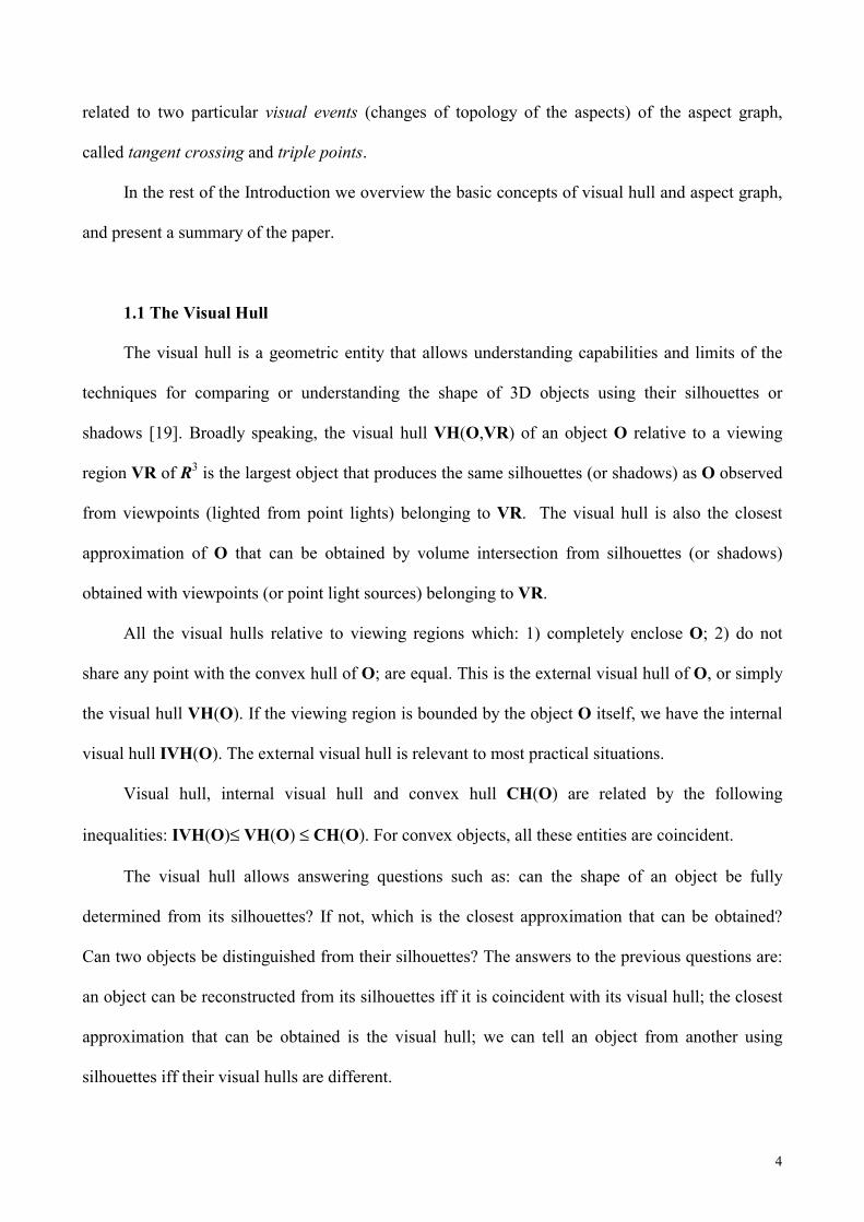
An intuitive physical construction of the visual hull of is as follows. Suppose filling the

concavities of the object with soft material. The visual hull can be obtained by scraping off the

excess material with a ruler grazing the hard surface of the object in all possible ways. In Fig.1, O is

one half of an object of revolution. CH(O) is its convex hull, where the concavity has been filled.

The last image shows the visual hull VH(O), and I particular S”VH, the surface of the visual hull

that covers the concavity, produced by the ruler.

Fig.1. An object O, its convex hull CH(O) and its visual hull VH(O)

Algorithms for computing the visual hulls of polygons, polyhedra and solids of revolution can

be found in [19], [20] and [27], to which the reader is referred for further details. Developments and

applications of the visual hull idea can be found in [21], [22] and [23].

1.2 The Aspect Graph

The basic idea of the aspect graph is clustering the infinite views of an object into a finite set

of representative views. The views to be clustered are the line drawings consisting of the occluding

contours and edges of the object image. For most viewpoints these views are topologically stable,

since perturbing the viewpoint in a small ball does not change their topological structure. The range

of all possible viewpoints can be partitioned into a set of maximal open regions where the structure

of the line drawing, also called aspect, is stable. Crossing the boundaries between these regions

produces a topological change in the aspects known as visual event. Aspects and visual events are

arranged into a graph structure, the aspect graph (AG), where each node is labeled with an aspect

and each arc represents a visual event. For perspective AG, each aspect corresponds to a connected

open volume of viewpoints, and each visual event to a boundary surface. For the parallel AG,

6

aspects and visual events correspond to open connected areas and boundary lines on the Gaussian

sphere. The parallel aspect graph is a sub-graph of the perspective aspect graph, since not any

perspective aspect is also a parallel aspect.

Constructing the AG requires determining the catalogue of the possible visual events and the

related boundary surfaces, which is relatively easy for planar faces object (see [14]). Several authors

have studied the more complex visual events of curved surfaces. A possible approach is using the

singularity theory for determining the visual events as the singularities of the visual mapping, which

maps the surface of the object onto the image plane [16], [15], [31], [32], [26], [5]. Other

approaches have also been used [11], [34]. For a comparison of the catalogues presented, the reader

is referred to [11]. Anyway, in this paper we will be only concerned with two simple and

universally recognized visual events.

Algorithms for constructing the aspect graphs have been given for polyhedra, articulated

objects, solids of revolution and various categories of curved objects under parallel and perspective

projection. For further details the reader is referred to the survey paper [3], to [4], [10], [11], [28],

[29] and [33], and to the comprehensive bibliography reported in these papers.

1.3 SUMMARY OF THE PAPER

The rest of this paper is organized as follows.

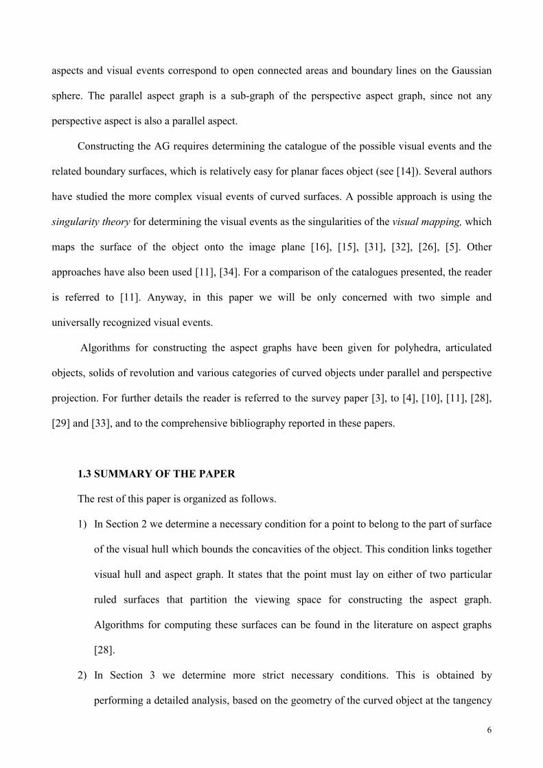
1) In Section 2 we determine a necessary condition for a point to belong to the part of surface

of the visual hull which bounds the concavities of the object. This condition links together

visual hull and aspect graph. It states that the point must lay on either of two particular

ruled surfaces that partition the viewing space for constructing the aspect graph.

Algorithms for computing these surfaces can be found in the literature on aspect graphs

[28].

2) In Section 3 we determine more strict necessary conditions. This is obtained by

performing a detailed analysis, based on the geometry of the curved object at the tangency

7

points of these surfaces. This analysis allows discarding entirely several of these surfaces

or in any cases some of their parts. The patches that survive this elimination process are

called locally active.

3) In Section 4 we sketch an algorithm for computing the visual hull, based on the locally

active patches.

2 A NECESSARY CONDITION FOR A POINT TO BELONG TO THE SURFACE OF

THE VISUAL HULL

Let us consider an object O bounded by a generic smooth surface. Obviously, the line

drawings of smooth objects only include occluding contours. The adjective “generic” refers to a

surface without exceptional zero probability alignments. This extends to curved surfaces the 2D

idea of generic polygon (three vertices do not lie on the same straight line) and the 3D idea of

generic polyhedron (two edges not belonging to the same face do not lie on the same plane, and

four edges do not lie on the same ruled quadric surface). In particular, generic for a smooth surface

means that there can exist only isolated lines (they do not form surfaces) tangent at more than three

points. For a more formal definition, the reader is referred to [7]. Aspect graphs and visual events of

generic smooth surfaces have been considered explicitly in several papers, as [5], [28], and

implicitly in many other papers on the subject.

In general, the surface SVH of VH(O) can be divided into two parts: S' VH coincident with the

surface S of O, and S”VH, which “covers” some concavities of O (see Fig.1 for an example).

Actually, S”VH could also bound volumes not connected to O (see [19]). In this section we will

relate S”VH to the boundary surfaces of the viewing space corresponding to two particular visual

events.

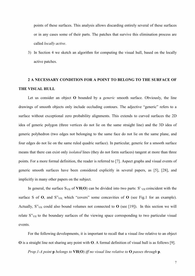
For the following developments, it is important to recall that a visual line relative to an object

O is a straight line not sharing any point with O. A formal definition of visual hull is as follows [9].

Prop.1-A point p belongs to VH(O) iff no visual line relative to O passes through p.

8

In the following we will use many times this condition for showing that a point does not

belong to the visual hull. From Prop.1 it follows that:

Prop.2- If a point p belongs to SVH, there are visual lines relative to O arbitrarily close to p.

From these statements we can derive a further necessary condition for a point to belong to

SVH.

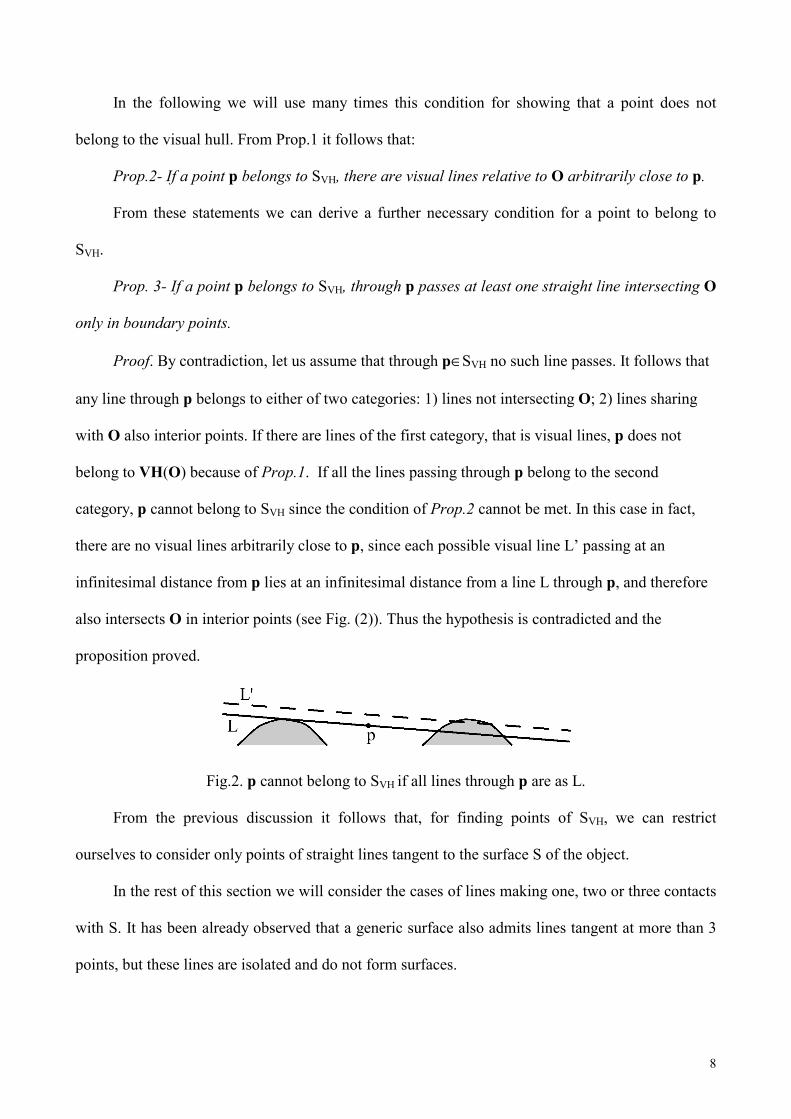
Prop. 3- If a point p belongs to SVH, through p passes at least one straight line intersecting O

only in boundary points.

Proof. By contradiction, let us assume that through p∈SVH no such line passes. It follows that

any line through p belongs to either of two categories: 1) lines not intersecting O; 2) lines sharing

with O also interior points. If there are lines of the first category, that is visual lines, p does not

belong to VH(O) because of Prop.1. If all the lines passing through p belong to the second

category, p cannot belong to SVH since the condition of Prop.2 cannot be met. In this case in fact,

there are no visual lines arbitrarily close to p, since each possible visual line L’ passing at an

infinitesimal distance from p lies at an infinitesimal distance from a line L through p, and therefore

also intersects O in interior points (see Fig. (2)). Thus the hypothesis is contradicted and the

proposition proved.

Fig.2. p cannot belong to SVH if all lines through p are as L.

From the previous discussion it follows that, for finding points of SVH, we can restrict

ourselves to consider only points of straight lines tangent to the surface S of the object.

In the rest of this section we will consider the cases of lines making one, two or three contacts

with S. It has been already observed that a generic surface also admits lines tangent at more than 3

points, but these lines are isolated and do not form surfaces.

9

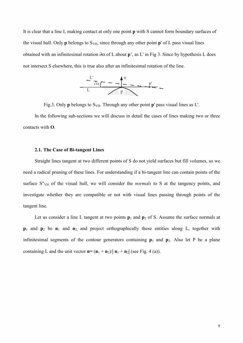
It is clear that a line L making contact at only one point p with S cannot form boundary surfaces of

the visual hull. Only p belongs to SVH, since through any other point p' of L pass visual lines

obtained with an infinitesimal rotation ∂α of L about p’, as L' in Fig 3. Since by hypothesis L does

not intersect S elsewhere, this is true also after an infinitesimal rotation of the line.

Fig.3. Only p belongs to SVH. Through any other point p' pass visual lines as L'.

In the following sub-sections we will discuss in detail the cases of lines making two or three

contacts with O.

2.1. The Case of Bi-tangent Lines

Straight lines tangent at two different points of S do not yield surfaces but fill volumes, so we

need a radical pruning of these lines. For understanding if a bi-tangent line can contain points of the

surface S"VH of the visual hull, we will consider the normals to S at the tangency points, and

investigate whether they are compatible or not with visual lines passing through points of the

tangent line.

Let us consider a line L tangent at two points p1 and p2 of S. Assume the surface normals at

p1 and p2 be n1 and n2, and project orthographically these entities along L, together with

infinitesimal segments of the contour generators containing p1 and p2. Also let P be a plane

containing L and the unit vector n= (n1 + n2)/| n1 + n2| (see Fig. 4 (a)).

10

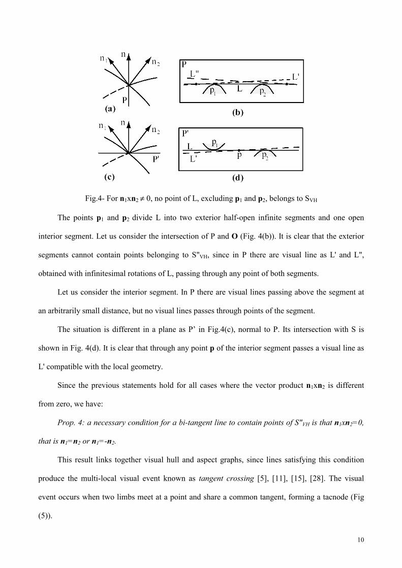
Fig.4- For n1xn2 ≠ 0, no point of L, excluding p1 and p2, belongs to SVH

The points p1 and p2 divide L into two exterior half-open infinite segments and one open

interior segment. Let us consider the intersection of P and O (Fig. 4(b)). It is clear that the exterior

segments cannot contain points belonging to S"VH, since in P there are visual line as L' and L",

obtained with infinitesimal rotations of L, passing through any point of both segments.

Let us consider the interior segment. In P there are visual lines passing above the segment at

an arbitrarily small distance, but no visual lines passes through points of the segment.

The situation is different in a plane as P’ in Fig.4(c), normal to P. Its intersection with S is

shown in Fig. 4(d). It is clear that through any point p of the interior segment passes a visual line as

L' compatible with the local geometry.

Since the previous statements hold for all cases where the vector product n1xn2 is different

from zero, we have:

Prop. 4: a necessary condition for a bi-tangent line to contain points of S"VH is that n1xn2=0,

that is n1=n2 or n1=-n2.

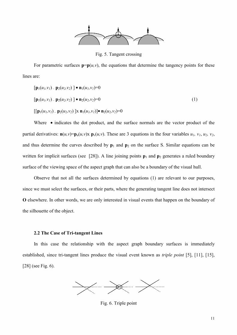
This result links together visual hull and aspect graphs, since lines satisfying this condition

produce the multi-local visual event known as tangent crossing [5], [11], [15], [28]. The visual

event occurs when two limbs meet at a point and share a common tangent, forming a tacnode (Fig

(5)).

11

Fig. 5. Tangent crossing

For parametric surfaces p=p(u,v), the equations that determine the tangency points for these

lines are:

[p1(u1,v1) – p2(u2,v2) ] • n1(u1,v1)=0

[p1(u1,v1) – p2(u2,v2) ] • n2(u2,v2)=0 (1)

[[p1(u1,v1) – p2(u2,v2) ]x n1(u1,v1)]• n2(u2,v2)=0

Where • indicates the dot product, and the surface normals are the vector product of the

partial derivatives: n(u,v)=pu(u,v)x pv(u,v). These are 3 equations in the four variables u1, v1, u2, v2,

and thus determine the curves described by p1 and p2 on the surface S. Similar equations can be

written for implicit surfaces (see [28]). A line joining points p1 and p2 generates a ruled boundary

surface of the viewing space of the aspect graph that can also be a boundary of the visual hull.

Observe that not all the surfaces determined by equations (1) are relevant to our purposes,

since we must select the surfaces, or their parts, where the generating tangent line does not intersect

O elsewhere. In other words, we are only interested in visual events that happen on the boundary of

the silhouette of the object.

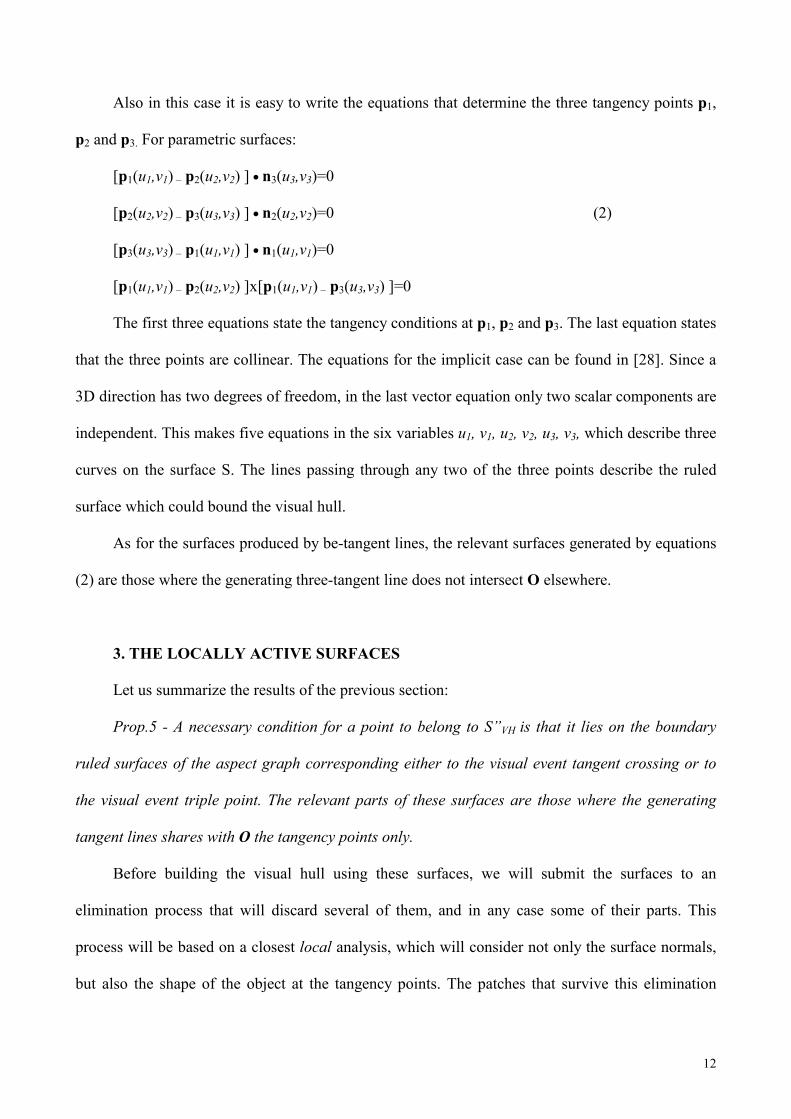
2.2 The Case of Tri-tangent Lines

In this case the relationship with the aspect graph boundary surfaces is immediately

established, since tri-tangent lines produce the visual event known as triple point [5], [11], [15],

[28] (see Fig. 6).

Fig. 6. Triple point

12

Also in this case it is easy to write the equations that determine the three tangency points p1,

p2 and p3. For parametric surfaces:

[p1(u1,v1) – p2(u2,v2) ] • n3(u3,v3)=0

[p2(u2,v2) – p3(u3,v3) ] • n2(u2,v2)=0 (2)

[p3(u3,v3) – p1(u1,v1) ] • n1(u1,v1)=0

[p1(u1,v1) – p2(u2,v2) ]x[p1(u1,v1) – p3(u3,v3) ]=0

The first three equations state the tangency conditions at p1, p2 and p3. The last equation states

that the three points are collinear. The equations for the implicit case can be found in [28]. Since a

3D direction has two degrees of freedom, in the last vector equation only two scalar components are

independent. This makes five equations in the six variables u1, v1, u2, v2, u3, v3, which describe three

curves on the surface S. The lines passing through any two of the three points describe the ruled

surface which could bound the visual hull.

As for the surfaces produced by be-tangent lines, the relevant surfaces generated by equations

(2) are those where the generating three-tangent line does not intersect O elsewhere.

3. THE LOCALLY ACTIVE SURFACES

Let us summarize the results of the previous section:

Prop.5 - A necessary condition for a point to belong to S”VH is that it lies on the boundary

ruled surfaces of the aspect graph corresponding either to the visual event tangent crossing or to

the visual event triple point. The relevant parts of these surfaces are those where the generating

tangent lines shares with O the tangency points only.

Before building the visual hull using these surfaces, we will submit the surfaces to an

elimination process that will discard several of them, and in any case some of their parts. This

process will be based on a closest local analysis, which will consider not only the surface normals,

but also the shape of the object at the tangency points. The patches that survive this elimination

13

process will be called locally active. This attribute will be applied also to the surfaces that contain

these patches and to the segments of straight lines that generate the surfaces.

The two following subsections will be devoted to determine the locally active patches

generated by bi-tangent and three-tangent lines

3.1 Locally Active Segments of Bi-tangent Lines

The technique that we will use for eliminating, completely or in part, tangent lines and the

surface they form, consists in finding, if they exist, visual lines passing through points of the

tangent line and compatible with the shape of the surface near the tangency point p1 and p2. For this

purpose, we will attempt to perform an infinitesimal rotation of the tangent line L about one of its

points without intersecting the infinitesimal surface patches near p1 and p2.

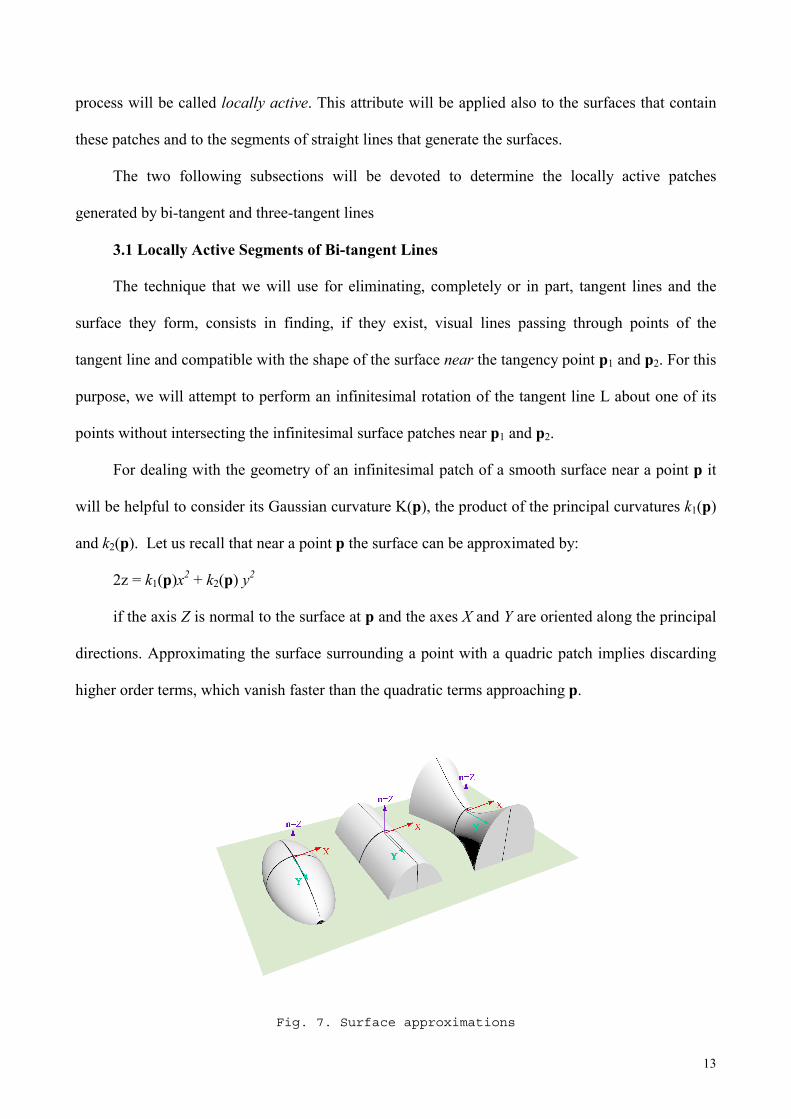
For dealing with the geometry of an infinitesimal patch of a smooth surface near a point p it

will be helpful to consider its Gaussian curvature K(p), the product of the principal curvatures k1(p)

and k2(p). Let us recall that near a point p the surface can be approximated by:

2z = k1(p)x2 + k2(p) y2

if the axis Z is normal to the surface at p and the axes X and Y are oriented along the principal

directions. Approximating the surface surrounding a point with a quadric patch implies discarding

higher order terms, which vanish faster than the quadratic terms approaching p.

Fig. 7. Surface approximations

14

This surface turns out to be: 1) a paraboloid if K(p)>0, 2) a saddle-shaped hyperboloid if

K(p)<0; 3) a cylinder if K(p)=0 and k1(p)=0, or k2(p)=0, but not both [25] (see Fig.7). We need not

to consider planar points where k1(p) = k2(p)=0, since generic surfaces can have only isolated planar

points. On a generic surface, points whose Gaussian curvature is strictly positive (elliptic points), or

strictly negative (hyperbolic points), forms open areas separated by curves whose points have zero

Gaussian curvature (parabolic points)[1], [28].

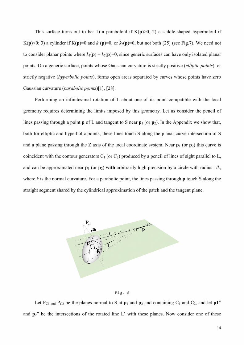
Performing an infinitesimal rotation of L about one of its point compatible with the local

geometry requires determining the limits imposed by this geometry. Let us consider the pencil of

lines passing through a point p of L and tangent to S near p1 (or p2). In the Appendix we show that,

both for elliptic and hyperbolic points, these lines touch S along the planar curve intersection of S

and a plane passing through the Z axis of the local coordinate system. Near p1 (or p2) this curve is

coincident with the contour generators C1 (or C2) produced by a pencil of lines of sight parallel to L,

and can be approximated near p1 (or p2) with arbitrarily high precision by a circle with radius 1/k,

where k is the normal curvature. For a parabolic point, the lines passing through p touch S along the

straight segment shared by the cylindrical approximation of the patch and the tangent plane.

Fig. 8

Let PC1 and PC2 be the planes normal to S at p1 and p2 and containing C1 and C2, and let p1”

and p2” be the intersections of the rotated line L’ with these planes. Now consider one of these

15

points, for instance p1”(Fig. 8). It is clear that L’ does not intersect S near p1 if p1” lies in PC1 on the

side of the contour generator marked by the external normal n1. Clearly, L’ is a visual line iff it is

possible to satisfy this condition at both the tangency points.

In the following we will consider separately the two cases n1= n2 and n1= -n2

3.1.1 Locally Active Segments for n1= n2

Observe first that only the interior segment of the tangent line could be locally active. This is

easily seen considering the section of O made by the plane PN containing n1 and n2. This section is

as that shown in Fig.4(b), and the same argument applies. Thus, we must only investigate the

interior segment.

The case n1= n2 generates six sub-cases, since each tangency point can be elliptic, parabolic

or hyperbolic. We will consider the sub-cases in the following order: elliptic-elliptic, parabolic -

elliptic, parabolic-parabolic, hyperbolic-parabolic, hyperbolic-hyperbolic, and hyperbolic-elliptic.

For each sub-case we show a figure containing:

• the tangent line L and, if it exists, the visual line L’ obtained by a rotation of L about one

of its points p;

• the tangency points p1 and p2 of L and the corresponding surface normals n1 and n2;

• two segments of paraboloid, hyperboloid, or cylinder according to the Gaussian curvature

at p1 and p2 cut by planes parallel to PT;

• the plane PT tangent at p1 and p2;

• the planes PC1 and PC2 containing C1 and C2 near p1 and p2;

• the intersections p1” and p2” of L’ and PC1 and PC2.

For each case we will show a perspective view of these entities, and an orthographic

projection along L onto a plane P. For simplicity, in the perspective view we omit PT, and in P the

entities projected will be indicated with the symbols of their 3D counterparts. The direction of the

projectors is always from p2 to p1.

16

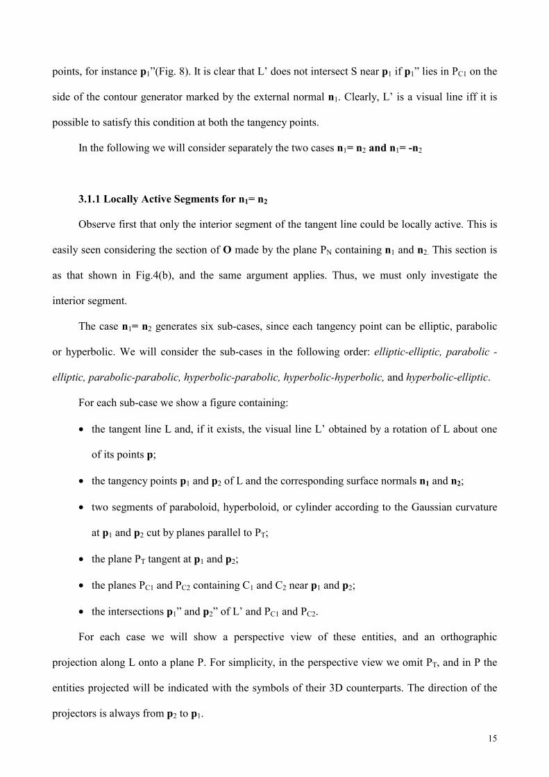
The sub-case elliptic-elliptic

Let us consider a point p of the interior segment (Fig. 9). Clearly an infinitesimal rotation δα

of L about p in the tangent plane PT generates a visual line L’, since both p1” and p2” lie on the

external side of C1 and C2, as shown by their projections onto the plane P. Therefore, the interior

segment is not locally active.

Fig. 9

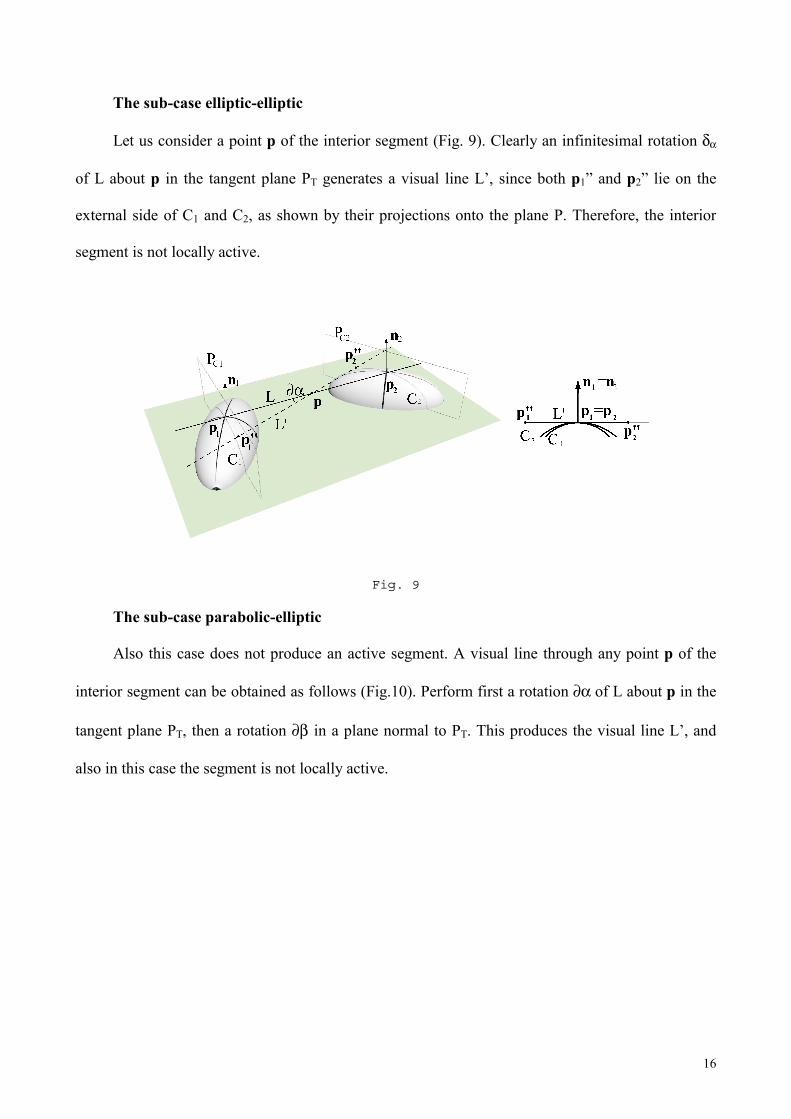
The sub-case parabolic-elliptic

Also this case does not produce an active segment. A visual line through any point p of the

interior segment can be obtained as follows (Fig.10). Perform first a rotation ∂α of L about p in the

tangent plane PT, then a rotation ∂β in a plane normal to PT. This produces the visual line L’, and

also in this case the segment is not locally active.

17

Fig. 10

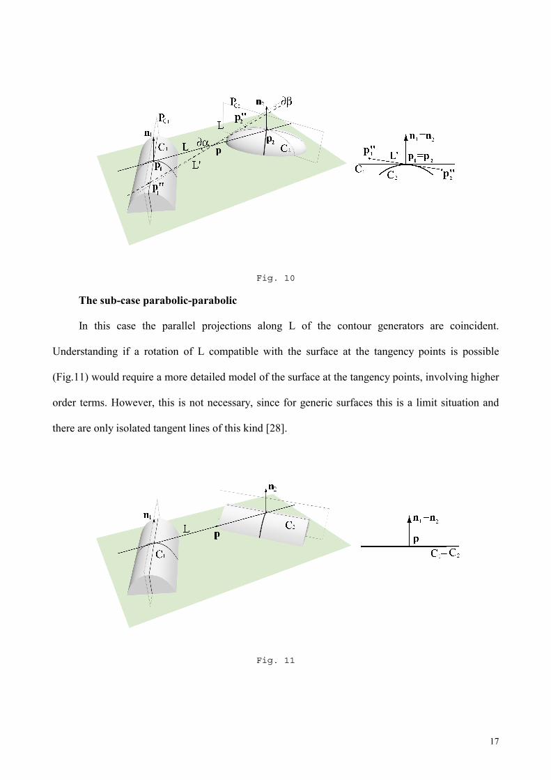
The sub-case parabolic-parabolic

In this case the parallel projections along L of the contour generators are coincident.

Understanding if a rotation of L compatible with the surface at the tangency points is possible

(Fig.11) would require a more detailed model of the surface at the tangency points, involving higher

order terms. However, this is not necessary, since for generic surfaces this is a limit situation and

there are only isolated tangent lines of this kind [28].

Fig. 11

18

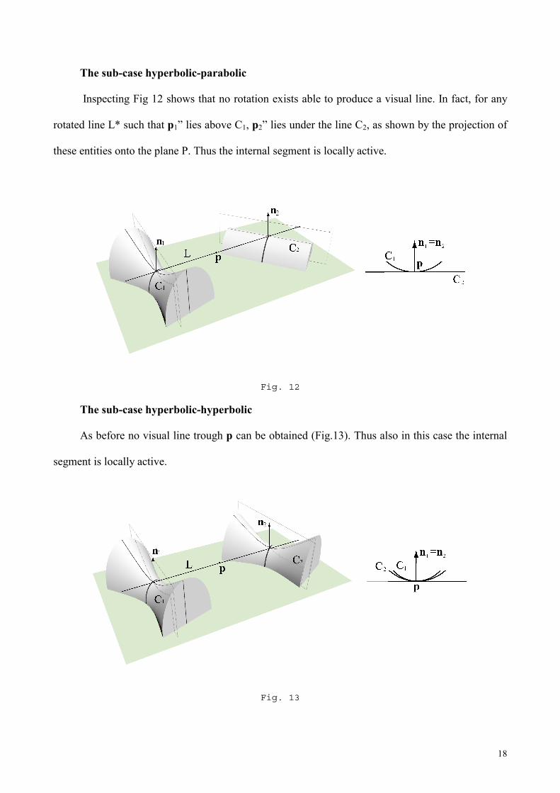
The sub-case hyperbolic-parabolic

Inspecting Fig 12 shows that no rotation exists able to produce a visual line. In fact, for any

rotated line L* such that p1” lies above C1, p2” lies under the line C2, as shown by the projection of

these entities onto the plane P. Thus the internal segment is locally active.

Fig. 12

The sub-case hyperbolic-hyperbolic

As before no visual line trough p can be obtained (Fig.13). Thus also in this case the internal

segment is locally active.

Fig. 13

19

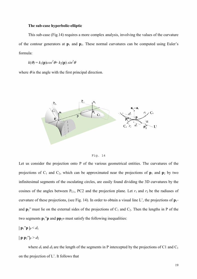
The sub-case hyperbolic-elliptic

This sub-case (Fig.14) requires a more complex analysis, involving the values of the curvature

of the contour generators at p1 and p2. These normal curvatures can be computed using Euler’s

formula:

k(θ) = k1(p)cos2θ+ k2(p) sin2θ

where θ is the angle with the first principal direction.

Fig. 14

Let us consider the projection onto P of the various geometrical entities. The curvatures of the

projections of C1 and C2, which can be approximated near the projections of p1 and p2 by two

infinitesimal segments of the osculating circles, are easily found dividing the 3D curvatures by the

cosines of the angles between PC1, PC2 and the projection plane. Let r1 and r2 be the radiuses of

curvature of these projections, (see Fig. 14). In order to obtain a visual line L’, the projections of p1”

and p2” must lie on the external sides of the projections of C1 and C2. Then the lengths in P of the

two segments p1”p and pp2» must satisfy the following inequalities:

| p1”p |P < d1

| p p2”|P > d2

where d1 and d2 are the length of the segments in P intercepted by the projections of C1 and C1

on the projection of L’. It follows that

20

| p1”p |P /| p p2”|P < d1/ d2 (*)

Let |p1p| and |p2p| be the finite 3D distances between p and the tangency points p1 and p2 (see Fig.

14). We have

| p1”p | P /| p p2”| P = |p1p| / |p2p|

In addition, for any angle α it is

d1/ d2 = r1 /r2

Then (*) becomes

|p1p| / |p2p| < r1 /r2 (**)

Concluding, only through points that satisfy (**) pass visual lines compatible with the local

geometry. It follows that the internal segment of L’ consists of an inactive segment p1p* and a

locally active segment near p*p2 such that

|p1p*| / | p*p2| = r1 /r2

3.2 Locally Active Segments of Bi-tangent Lines for n1= -n2

Observe first that only the exterior half-open segments can be locally active. This is

immediately seen by inspecting the section of O made by the plane PN containing n1 and n2, as can

be seen in Fig.4(d). Thus we must only investigate the two external half-open segments.

The possible cases are six as before. For brevity, will not report here a detailed analysis for

the first five cases, since they are similar to the corresponding cases of the previous subsection.

The results are as follows. The cases elliptic-elliptic and elliptic-parabolic are not active. As

before, it is not necessary to deal with the case parabolic-parabolic. Both the cases parabolic-

hyperbolic and hyperbolic-hyperbolic produce locally active exterior segments.

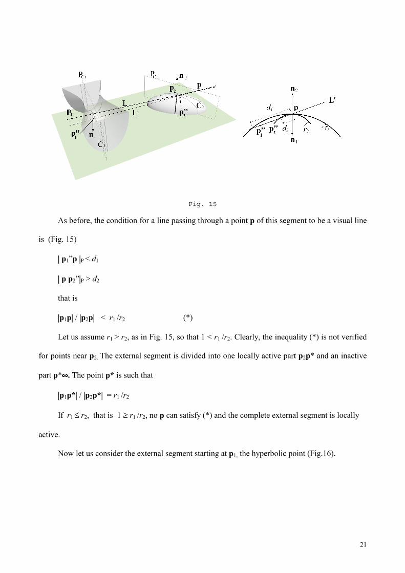
As in the previous section, the case hyperbolic-elliptic requires a detailed analysis involving

the curvatures of the contour generators. Let us consider first (Fig.15) the external segment starting

at p2, the elliptic point.

21

Fig. 15

As before, the condition for a line passing through a point p of this segment to be a visual line

is (Fig. 15)

| p1”p |P < d1

| p p2”|P > d2

that is

|p1p| / |p2p| < r1 /r2 (*)

Let us assume r1 > r2, as in Fig. 15, so that 1 < r1 /r2. Clearly, the inequality (*) is not verified

for points near p2. The external segment is divided into one locally active part p2p* and an inactive

part p*∞∞∞∞. The point p* is such that

|p1p*| / |p2p*| = r1 /r2

If r1 ≤ r2, that is 1 ≥ r1 /r2, no p can satisfy (*) and the complete external segment is locally

active.

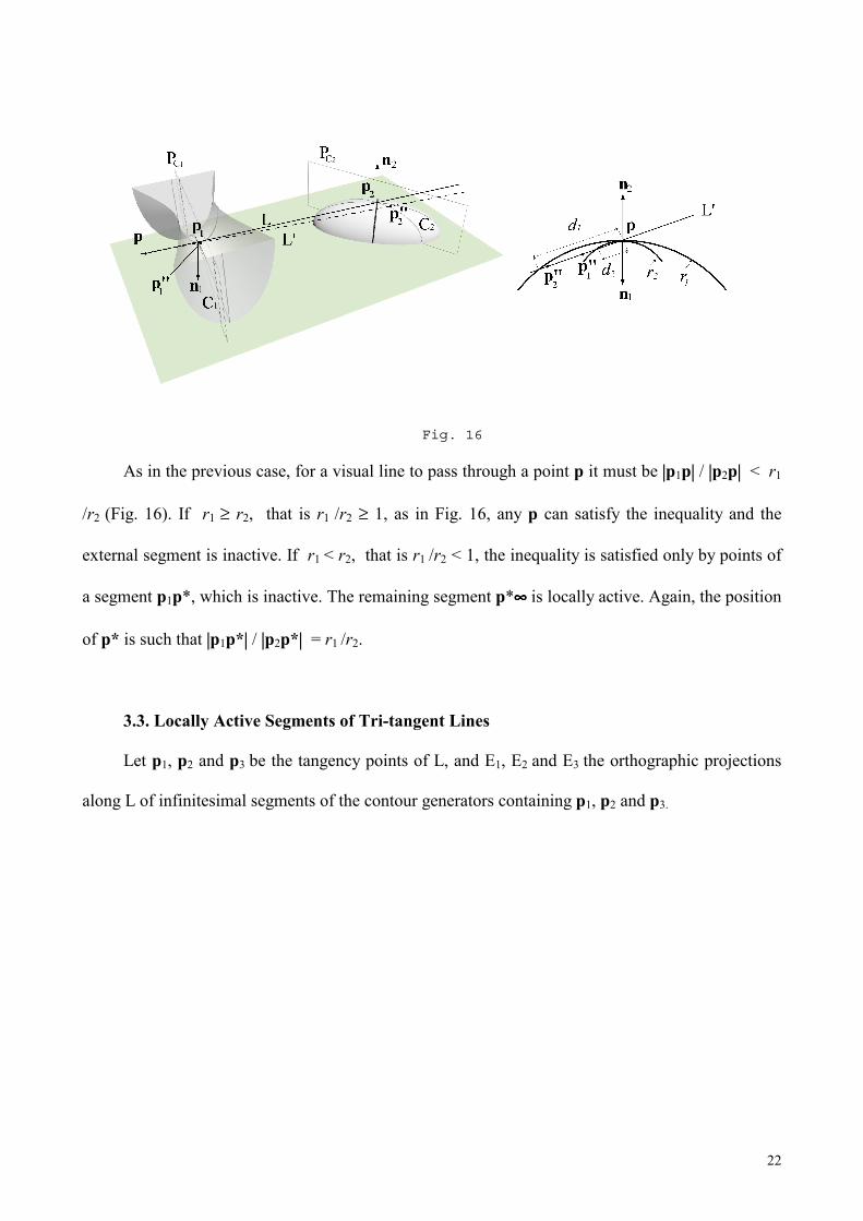
Now let us consider the external segment starting at p1, the hyperbolic point (Fig.16).

22

Fig. 16

As in the previous case, for a visual line to pass through a point p it must be |p1p| / |p2p| < r1

/r2 (Fig. 16). If r1 ≥ r2, that is r1 /r2 ≥ 1, as in Fig. 16, any p can satisfy the inequality and the

external segment is inactive. If r1 < r2, that is r1 /r2 < 1, the inequality is satisfied only by points of

a segment p1p*, which is inactive. The remaining segment p*∞∞∞∞ is locally active. Again, the position

of p* is such that |p1p*| / |p2p*| = r1 /r2.

3.3. Locally Active Segments of Tri-tangent Lines

Let p1, p2 and p3 be the tangency points of L, and E1, E2 and E3 the orthographic projections

along L of infinitesimal segments of the contour generators containing p1, p2 and p3.

23

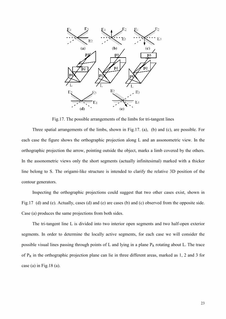
Fig.17. The possible arrangements of the limbs for tri-tangent lines

Three spatial arrangements of the limbs, shown in Fig.17. (a), (b) and (c), are possible. For

each case the figure shows the orthographic projection along L and an assonometric view. In the

orthographic projection the arrow, pointing outside the object, marks a limb covered by the others.

In the assonometric views only the short segments (actually infinitesimal) marked with a thicker

line belong to S. The origami-like structure is intended to clarify the relative 3D position of the

contour generators.

Inspecting the orthographic projections could suggest that two other cases exist, shown in

Fig.17 (d) and (e). Actually, cases (d) and (e) are cases (b) and (c) observed from the opposite side.

Case (a) produces the same projections from both sides.

The tri-tangent line L is divided into two interior open segments and two half-open exterior

segments. In order to determine the locally active segments, for each case we will consider the

possible visual lines passing through points of L and lying in a plane PR rotating about L. The trace

of PR in the orthographic projection plane can lie in three different areas, marked as 1, 2 and 3 for

case (a) in Fig.18 (a).

24

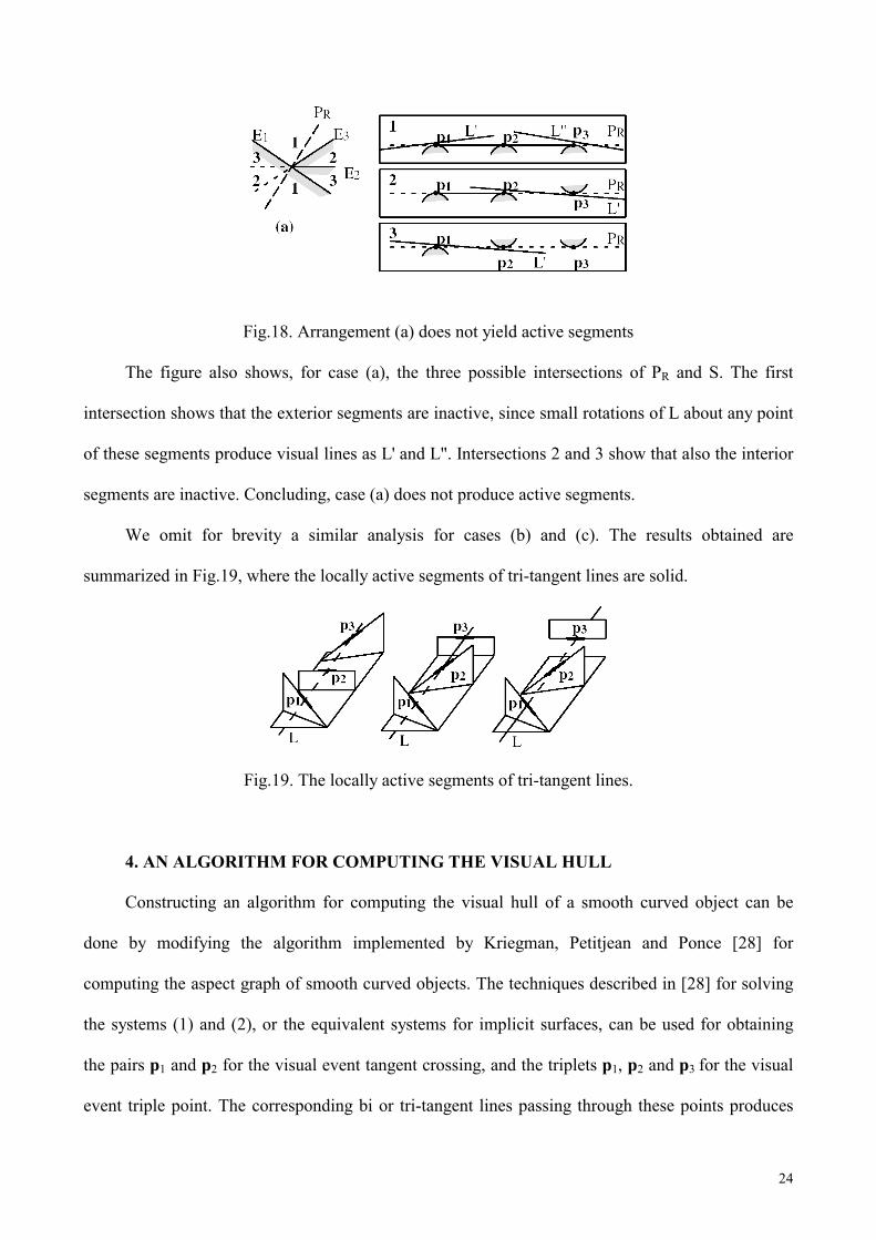
Fig.18. Arrangement (a) does not yield active segments

The figure also shows, for case (a), the three possible intersections of PR and S. The first

intersection shows that the exterior segments are inactive, since small rotations of L about any point

of these segments produce visual lines as L' and L". Intersections 2 and 3 show that also the interior

segments are inactive. Concluding, case (a) does not produce active segments.

We omit for brevity a similar analysis for cases (b) and (c). The results obtained are

summarized in Fig.19, where the locally active segments of tri-tangent lines are solid.

Fig.19. The locally active segments of tri-tangent lines.

4. AN ALGORITHM FOR COMPUTING THE VISUAL HULL

Constructing an algorithm for computing the visual hull of a smooth curved object can be

done by modifying the algorithm implemented by Kriegman, Petitjean and Ponce [28] for

computing the aspect graph of smooth curved objects. The techniques described in [28] for solving

the systems (1) and (2), or the equivalent systems for implicit surfaces, can be used for obtaining

the pairs p1 and p2 for the visual event tangent crossing, and the triplets p1, p2 and p3 for the visual

event triple point. The corresponding bi or tri-tangent lines passing through these points produces

25

the relevant boundary surfaces. For obtaining the locally active patches, we must discard the

surfaces, or their parts, which:

1) do not satisfy the local necessary conditions determined in Section 3;

2) intersect S.

By intersecting all the locally active patches we construct a partition of R3. Each cell of this

partition belongs entirely or does not belong at all to the visual hull, and the whole visual hull can

be constructed by checking each cell and merging with O those belonging to the visual hull. To

check a cell, chose a random point in it, and construct the cone formed by the lines passing through

the point and tangent to O. The cell belongs to the visual hull if all the tangent lines also intersect

O.

The complexity of the visual hull algorithm is bounded by the complexity of the algorithm for

computing the perspective aspect graph. For algebraic surfaces of degree g, it has been found [29]

that this complexity is O(g18 ), due to the tri-tangent surfaces.

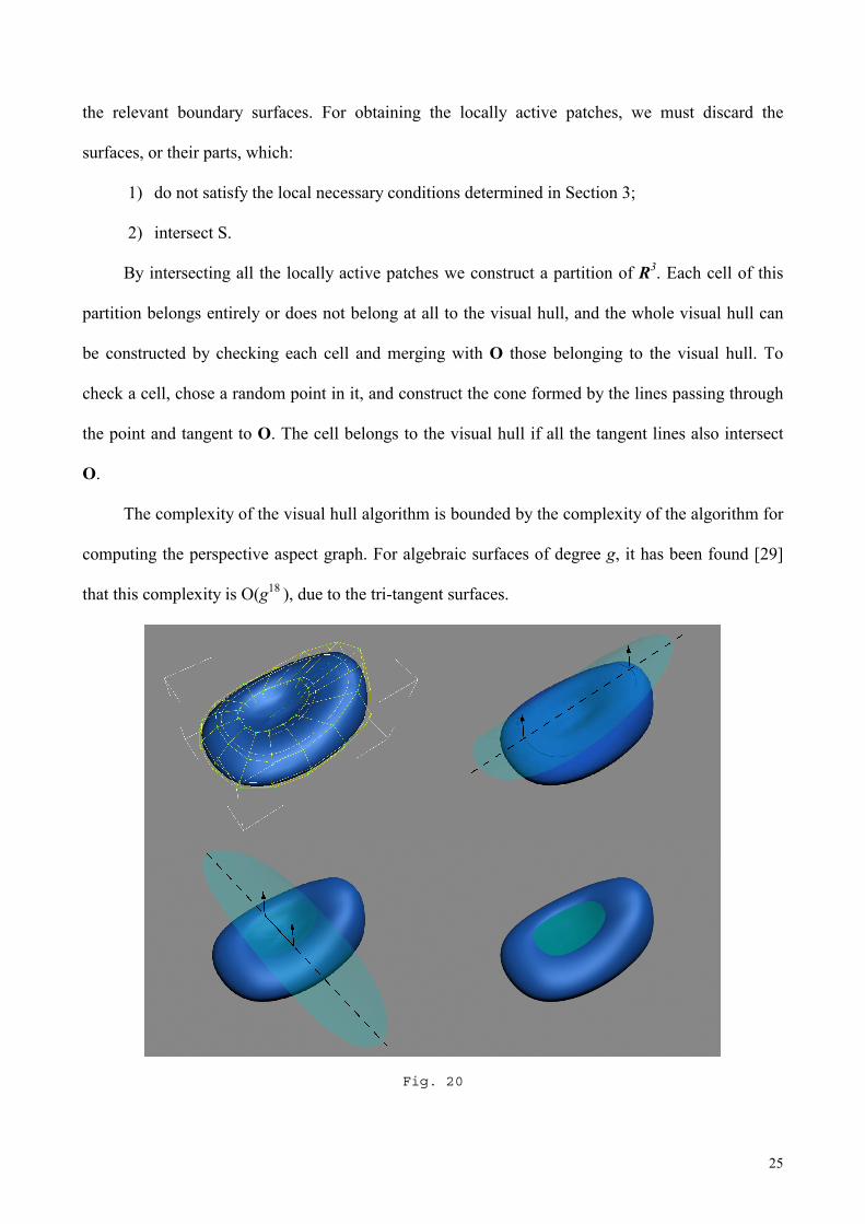
Fig. 20

26

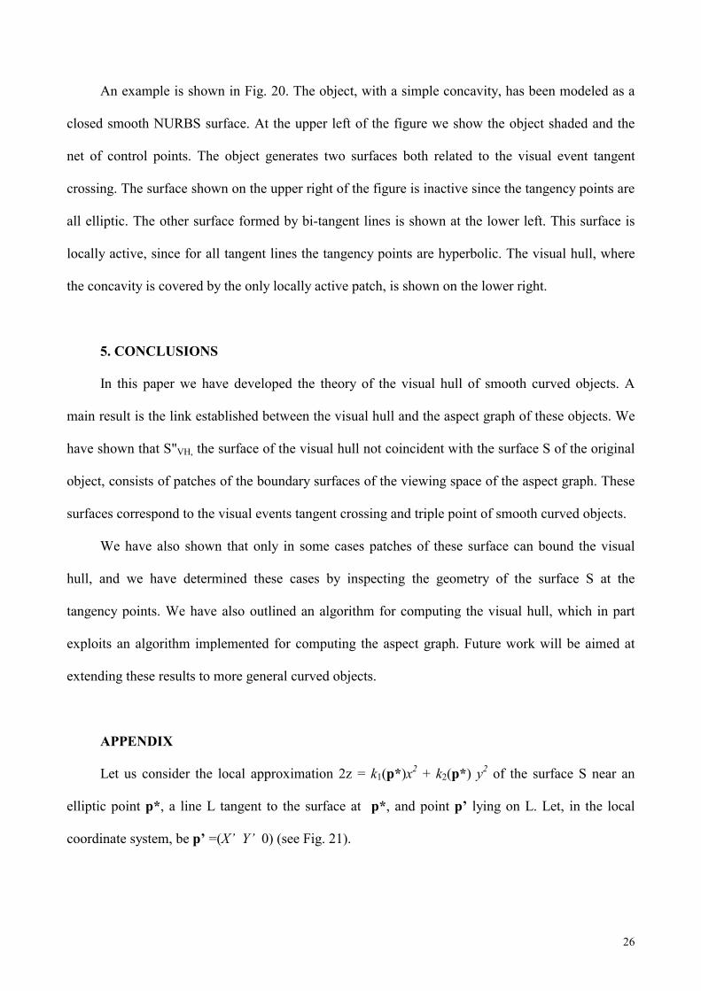
An example is shown in Fig. 20. The object, with a simple concavity, has been modeled as a

closed smooth NURBS surface. At the upper left of the figure we show the object shaded and the

net of control points. The object generates two surfaces both related to the visual event tangent

crossing. The surface shown on the upper right of the figure is inactive since the tangency points are

all elliptic. The other surface formed by bi-tangent lines is shown at the lower left. This surface is

locally active, since for all tangent lines the tangency points are hyperbolic. The visual hull, where

the concavity is covered by the only locally active patch, is shown on the lower right.

5. CONCLUSIONS

In this paper we have developed the theory of the visual hull of smooth curved objects. A

main result is the link established between the visual hull and the aspect graph of these objects. We

have shown that S"VH, the surface of the visual hull not coincident with the surface S of the original

object, consists of patches of the boundary surfaces of the viewing space of the aspect graph. These

surfaces correspond to the visual events tangent crossing and triple point of smooth curved objects.

We have also shown that only in some cases patches of these surface can bound the visual

hull, and we have determined these cases by inspecting the geometry of the surface S at the

tangency points. We have also outlined an algorithm for computing the visual hull, which in part

exploits an algorithm implemented for computing the aspect graph. Future work will be aimed at

extending these results to more general curved objects.

APPENDIX

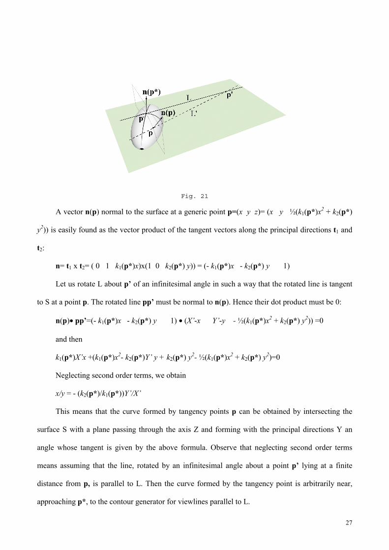
Let us consider the local approximation 2z = k1(p*)x2 + k2(p*) y2 of the surface S near an

elliptic point p*, a line L tangent to the surface at p*, and point p’ lying on L. Let, in the local

coordinate system, be p’ =(X’ Y’ 0) (see Fig. 21).

27

Fig. 21

A vector n(p) normal to the surface at a generic point p=(x y z)= (x y ½(k1(p*)x2 + k2(p*)

y2)) is easily found as the vector product of the tangent vectors along the principal directions t1 and

t2:

n= t1 x t2= ( 0 1 k1(p*)x)x(1 0 k2(p*) y)) = (- k1(p*)x - k2(p*) y 1)

Let us rotate L about p’ of an infinitesimal angle in such a way that the rotated line is tangent

to S at a point p. The rotated line pp’ must be normal to n(p). Hence their dot product must be 0:

n(p)• pp’=(- k1(p*)x - k2(p*) y 1) • (X’-x Y’-y - ½(k1(p*)x2 + k2(p*) y2)) =0

and then

k1(p*)X’x +(k1(p*)x2- k2(p*)Y’ y + k2(p*) y2- ½(k1(p*)x2 + k2(p*) y2)=0

Neglecting second order terms, we obtain

x/y = - (k2(p*)/k1(p*))Y’/X’

This means that the curve formed by tangency points p can be obtained by intersecting the

surface S with a plane passing through the axis Z and forming with the principal directions Y an

angle whose tangent is given by the above formula. Observe that neglecting second order terms

means assuming that the line, rotated by an infinitesimal angle about a point p’ lying at a finite

distance from p, is parallel to L. Then the curve formed by the tangency point is arbitrarily near,

approaching p*, to the contour generator for viewlines parallel to L.

28

The above results also hold for an hyperbolic point. The only difference is that, since the

principal curvatures have opposite signs, in the plane XY the line L and the trace of the plane

containing the contact curve are in the same quadrant.

6. REFERENCES

[1] N. Ahuja and J. Veenstra: Generating octrees from object silhouettes in orthographic views,

IEEE Trans. on PAMI,Vol.11,pp.137-149,1989

[2] V.I.Arnold, Catastrophe Theory, Springer-Verlag, Heidelberg,1984

[3] K.W. Bowyer and C.R. Dyer, “Aspect Graphs: An Introduction and Survey of Recent Results,”

Int’l J. Imaging Systems and Technology, vol.2, pp. 315-328, 1990

[4] K.Bowyer , M. Sallam, D.Eggert and J. Stewman, “Computing the Generalized Aspect Graph

for Objects with Moving Parts,” IEEE Trans. Pattern Analysis and Machine Intelligence, vol.15,

no.6, pp.605-610, 1993

[5] J.Callahan and R. Weiss, ”A Model for Describing Surface Shape,” in Proc. IEEE Conf. on

Comp. Vision and Pattern Recognition, pp. 240-245, 1985

[6] C. H. Chian and J. K. Aggarwal: Model reconstruction and shape recognition from occluding

contours", IEEE Trans.on PAMI, Vol.11, pp.372-389, 1989

[7] M. Demazure, “Catastrophes et bifurcations,”Edition Ellipses, 1989

[8] F. Durand, G. Drettakis and C. Puech, “The 3D visibility complex: a unified data-structure for

global visibility of scenes of polygons and smooth objects,” Proc. 9th Canadian Conference on

Comput. Geometry, Kingston, Canada, pp. 153-158, 1997

[9] F. Durand, G. Drettakis and C. Puech, “The 3D visibility complex ,”ACM Trans. On Graphics,

Vol. 21. no.2, pp.176-206, 2002

29

[10] D.W. Eggert , K.W. Bowyer, C.R. Dyer, H.I. Christensen, and D.B. Goldof, “The Scale Space

Aspect Graph, ”IEEE Trans. Pattern Analysis and Machine Intelligence, vol.15, no.11, pp.1,114-

1139, 1993

[11] D.Eggert and K.Bowyer,” Computing the Perspective Aspect Graph of Solids of

Revolution,”IEEE Trans. Pattern Analysis and Machine Intelligence, vol.15, no.2, pp.109-128,

1993

[12] D. A. Forsyth, “Recognizing algebraic surfaces from their outlines,” Int. J. of Computer

Vision, vol. 18, no.1, pp.21-40, 1996

[13] J.J. Gibson, “What is a form?” Psychol. Rev., vol.58, pp. 403-412, 1951

[14] Z.Gigus, J.Canny, and R. Seidel, “Efficiently computing and representing aspect graphs of

polyhedral objects,” ,” IEEE Trans. Pattern Analysis and Machine Intelligence, vol.13, no.6, pp.

542-551, 1991

[15] Y.K. Kergosien,”La Famille des Projections Orthogonales d’Une Surface et Ses Singularités,”

C.R. Acad.Sc.Paris, 292, pp.929-932, 1981

[16] J. J.Koenderink and A. J. van Doorn," The Singularities of the Visual Mapping," Biol. Cybern.

vol.24, pp.51-59, 1976

[17] J. J.Koenderink and A. J. van Doorn," The Internal Representation of Solid Shapes with

Respect to Vision," Biol. Cybern. vol.32, pp.211-216, 1979

[18] D.J. Kriegman and J.Ponce, “On recognizing and positioning curved 3D objects from image

contours,” IEEE Trans. Pattern Analysis and Machine Intelligence, vol.12, no.12, pp.1127-1137,

1990

[19] A. Laurentini," The Visual Hull Concept for Silhouette-based Image Understanding," IEEE

Trans. Pattern Analysis and Machine Intelligence,vol.16, pp.150-162, 199

[20] A. Laurentini, "Computing the Visual Hull of Solids of Revolution," Pattern Recognition, vol.

32, pp.377-388, 1999

30

[21] A. Laurentini ," How Far 3-D Shapes Can Be Understood from 2-D Silhouettes," IEEE Trans.

Pattern Analysis and Machine Intelligence, vol. 17, pp.188-195, 1995

[22] A. Laurentini, "Surface Reconstruction Accuracy for Active Volume Intersection," Pattern

Recognition Letters, vol. 17, pp. 1285-1292, 1996

[23] A. Laurentini," How Many 2D Silhouettes it Takes to Reconstruct a 3D Object," Comput.

Vision and Image Understanding, vol.67, pp. 81-87, 1997

[24] P. Mendonca, K.Wong and R. Cipolla, ”Epipolar geometry from profiles under circular

motion,” IEEE Trans. Pattern Analysis and Machine Intelligence, vol. 23, pp.604-616, 2001

[25] B.O'Neill, Elementary Differential Geometry, Academic Press, San Diego, 1996

[26] O.A. Platonova, ”Singularities of projections of smooth surfaces,” Russian Math. Surveys, . 39,

pp.177-178, 1984

[27] S. Petitjean,"A Computational Geometric Approach to Visual Hull," Int. J. of Comput.

Geometry and Appl., vol. 8, no.4, pp. 407-436, 1998

[28] S.Petitjean, J.Ponce and D.J.Kriegman, "Computing exact aspect graphs of curved objects:

algebraic surfaces," Int. J. of Computer Vision, vol. 9, no.3, pp.231-255, 1992

[29] S.Petitjean,” The enumerative geometry of projective algebraic surfaces and the complexity of

aspect graphs,” Int. J. of Computer Vision, vol. 19, pp.1-29, 1996

[30]M. Pocchiola and G. Vegter, “The Visibility Complex,” Int. J. of Comput. Geometry and Appl.,

vol. 6, no.3, pp. 279-308, 1996

[31] J. Rieger, “On the classification of views of piecewise smooth objects,” Image Vis. Comput.

Vol.5, pp. 91-97, 1987

[32] J. Rieger, “The geometry of view space of opaque objects bounded by smooth surfaces,”

Artificial Intelligence, Vol. 44, pp. 1-40, 1990

[33] I. Shimshoni and J.Ponce, “Finite Resolution Aspect Graphs of Polyhedral Objects,” IEEE

Trans. Pattern Analysis and Machine Intelligence, vol.19, no.4, pp.315-327, 1997

31

[34] T. Sripradisvarakul and R. Jain,” Generating aspect graphs for curved objects,” Proc. IEEE.

Workshop on Interpretation of 3D Scenes, pp. 109-115,1989

[35] J. Y. Zheng: Acquiring 3D models from sequences of contours, IEEE Trans. on PAMI, Vol.

16, no.2, pp.163-178,1994