Embed Size (px)
Citation preview

IB GEOGRAPHY INTERNAL ASSESSMENT
The Waitakere River A Fieldwork Investigation into the Discharge of
the Waitakere River
Simon Johnson
Kristin School, New Zealand
000434-051
Word Count: 2515

- 2 -
Contents Page

- 3 -

- 4 -
Introduction
The aim of this investigation is to determine how far the hypothesis “that the discharge of a river will
increase downstream and will vary markedly between seasons” is true for a relatively small drainage
basin. Discharge is defined as the amount of water passing a given survey point in a given time.
Measured in cumecs, it gives an indication as to how much water is in the river, and how close it is to
bank-full state. In order to test how far the hypothesis is true for a small scale river basin, 5 sites along
the Waitakere River will be tested and the discharge will be compared, both between sites and between
seasons. It is foreseen that the discharge of the river will be significantly greater downstream for a
number of reasons. Firstly, as the river moves towards its mouth, more water will have entered the river
from tributaries increasing the discharge. Secondly, the amount of water originating from precipitation
will have increased from run-off from the surrounding land, a factor that can be exacerbated by human
activities such as deforestation or urbanisation. Equally, the reason that the discharge will vary between
seasons can be ascribed to the change in weather patterns. Discharge can be described as “the amount
of water originally from precipitation which reaches the channel….” (Waugh, 2005, p. 61.) In the winter,
one would expect the amount of discharge to be greater as the amount of precipitation would be
expected to be greater.
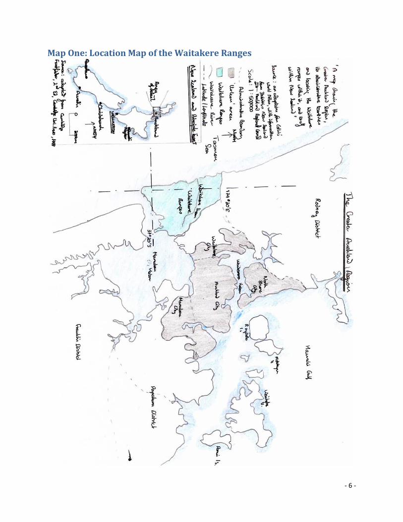
Background to the Waitakere Ranges
The Waitakere River and its drainage basin is the subject of this investigation. A small drainage basin,
located in the Waitakere Ranges approximately 25 kilometres west of Auckland City, New Zealand, it is
located within a Heritage Area, with very limited human construction. (McClure, 2008) To that end, the
discharge should not be significantly affected by either urbanisation or deforestation. The river itself is
fed by several tributaries, becoming an order 5 stream by the time it reaches the Tasman Sea. These
tributaries will provide with sufficient resources to test the theory that discharge increases closer to the
river mouth due to the increased number of tributaries.
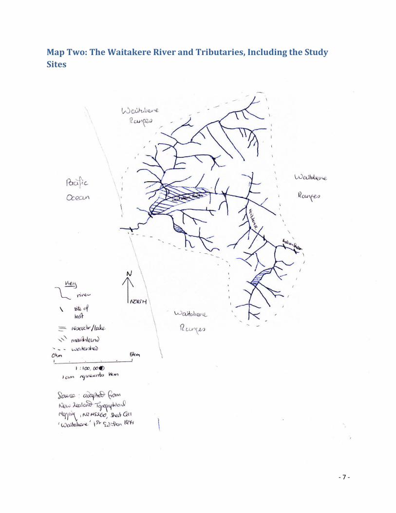
Methodology
For this investigation, 5 sites along the Waitakere River are to be measured. They have been selected
along the river, in the upper, middle and lower course to allow for comparison between them. The first
site is not at the head of the Waitakere River, but at one of its principle tributaries: the Anderson
Stream. This is because of the presence of the Waitakere Dam (see figure XX on page XX) which would
distort the discharge figures. The sites were chosen to be roughly equidistance between each other to
allow a graph to be drawn of the rate of change of the discharge. It’s worth noting, however, that the
choice of sites was constrained by the requirements of access to them. In order to compare the

- 5 -
seasons, the measurements are to be carried out on the 27th
August (the winter test) and 8th
March,
2009 (the summer test).
The object being to compare the discharge of the sites, both the velocity of the stream and the cross
sectional areas will be recorded at each site. The velocity will be gained by dropping an orange into the
stream, and recording the time taken to travel the distance chosen. It will then be calculated by dividing
the distance covered by the time taken. To calculate the cross sectional area, the depth of the river will
be measured at chosen intervals, and a mean gained. This will then be multiplied by the measured width
of the river. This is only an approximation, but is the best method obtainable under the field conditions.
In order to calculate the discharge, the velocity will be multiplied by the cross sectional area.
The hydraulic radius gives an impression of the river’s efficiency and is being calculated in order to
determine at what point on the rivers course the site is located at. It will be calculated by multiplying the
cross sectional area, as recorded above, to the whetted perimeter. This will be calculated by using a tape
measure held along bed and banks of the river. A Long Profile graph will confirm the results of the
hydraulic radius, as to the site’s position on the river’s course, and will recorded on a clinometer. Finally,
at each site, photographs and sketches will be drawn and notes taken, in order to note any factors that
may affect the discharge.
Outside of the field, the month to date rainfall will be obtained from the Auckland Regional Council
Weather station. This will be used to determine the amount of precipitation in the stream which may
affect the discharge calculations if extreme. The bifurcation ratio will also be calculated of the drainage
basin, in order to confirm the small size of the basin. In order to do this, the stream ordering will be
calculated and tallied. A ratio between each order will created and the average of the ratio’s serves as
the bifurcation ratio.
- 6 -
Map One: Location Map of the Waitakere Ranges
- 7 -
Map Two: The Waitakere River and Tributaries, Including the Study
Sites
- 8 -
Site One
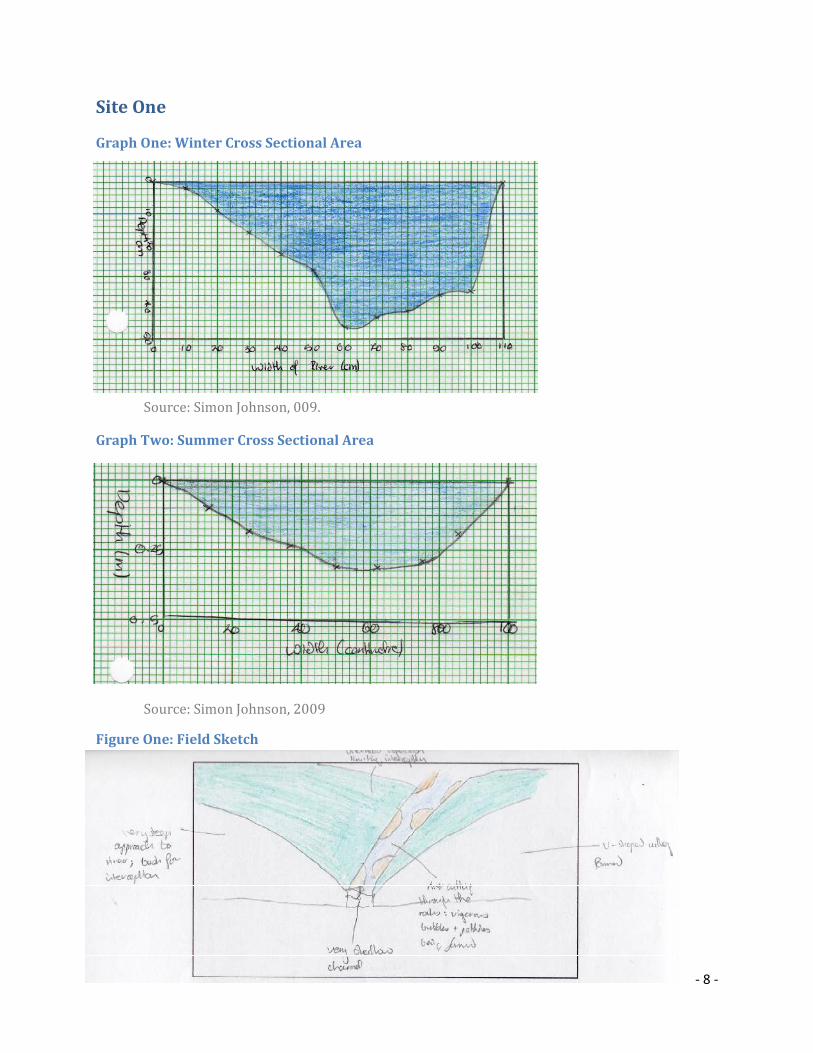
Graph One: Winter Cross Sectional Area
Source: Simon Johnson, 009.
Graph Two: Summer Cross Sectional Area
Source: Simon Johnson, 2009
Figure One: Field Sketch
- 9 -
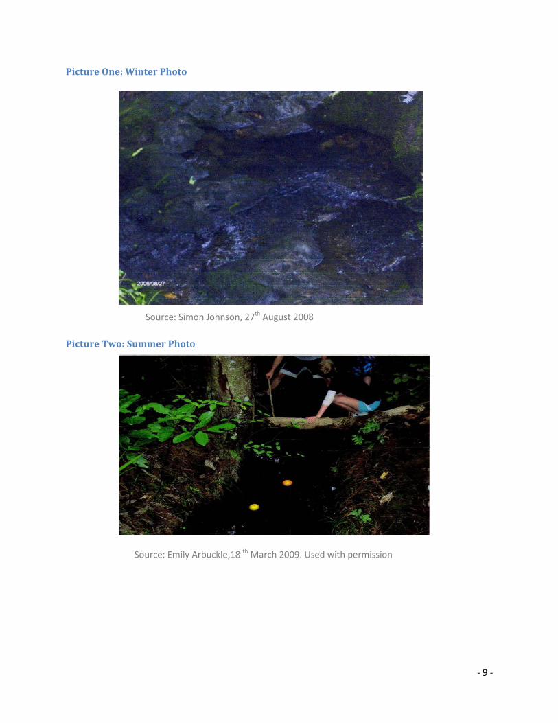
Picture One: Winter Photo
Picture Two: Summer Photo
Source: Simon Johnson, 27th
August 2008
Source: Emily Arbuckle,18 th
March 2009. Used with permission

- 10 -
- 11 -
Site Two
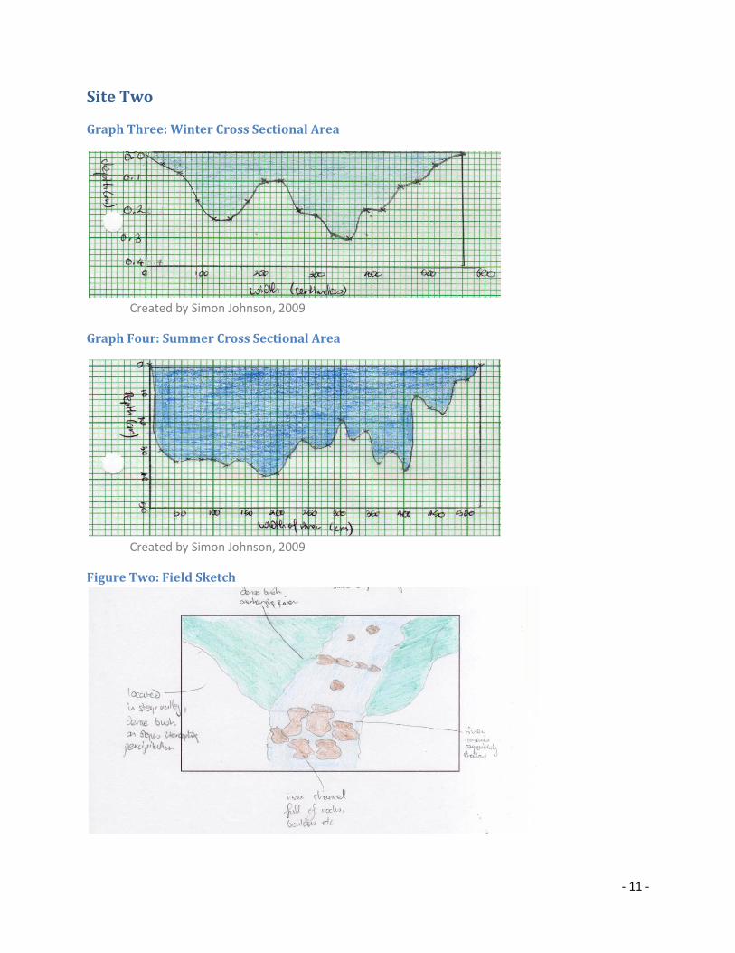
Graph Three: Winter Cross Sectional Area
Created by Simon Johnson, 2009
Graph Four: Summer Cross Sectional Area
Created by Simon Johnson, 2009
Figure Two: Field Sketch
- 12 -
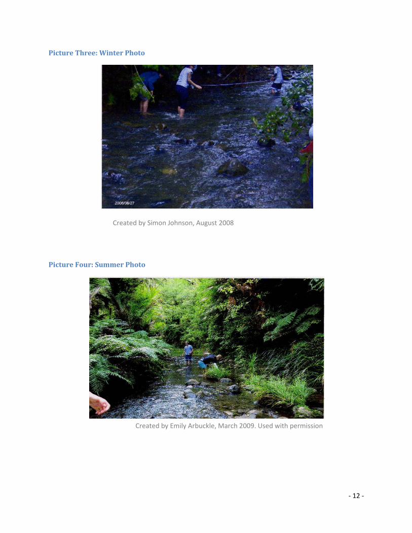
Picture Three: Winter Photo
Picture Four: Summer Photo
Created by Emily Arbuckle, March 2009. Used with permission
Created by Simon Johnson, August 2008
- 13 -
- 14 -
Site Three
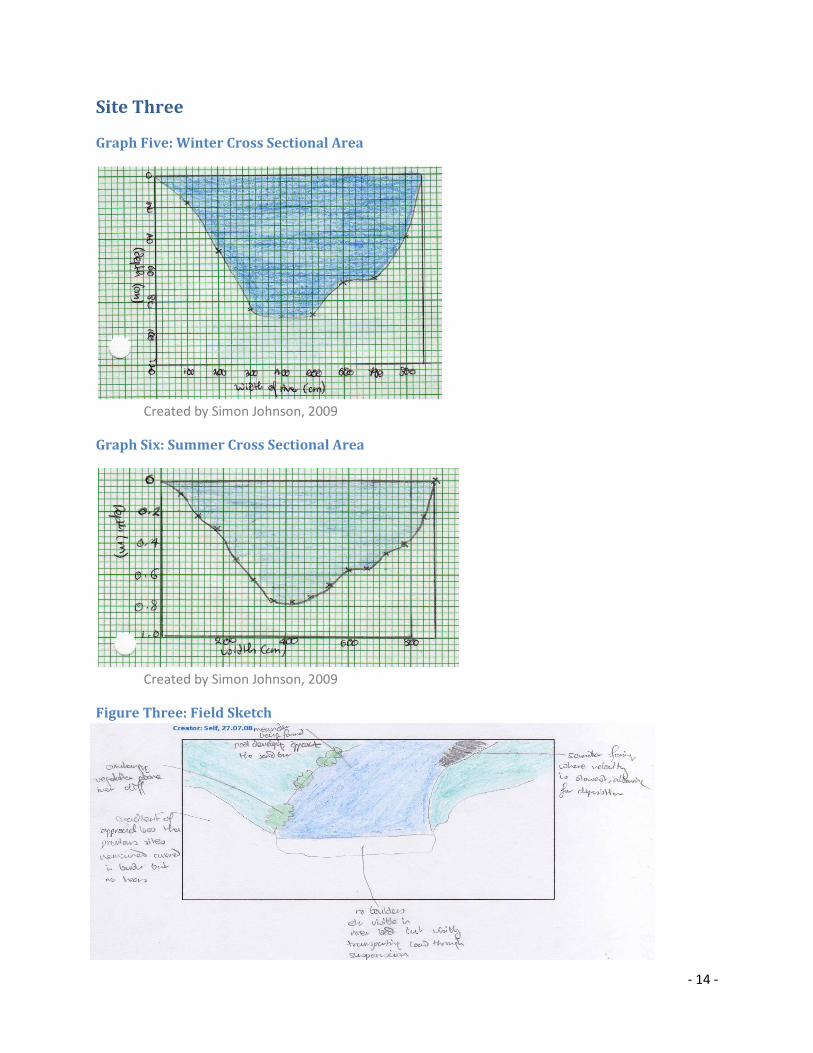
Graph Five: Winter Cross Sectional Area
Created by Simon Johnson, 2009
Graph Six: Summer Cross Sectional Area
Created by Simon Johnson, 2009
Figure Three: Field Sketch
- 15 -
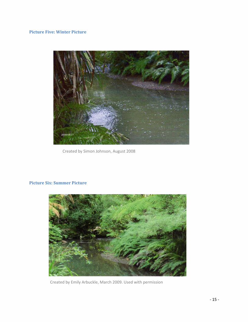
Picture Five: Winter Picture
Picture Six: Summer Picture
Created by Simon Johnson, August 2008
Created by Emily Arbuckle, March 2009. Used with permission
- 16 -
- 17 -
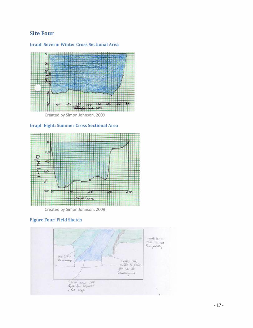
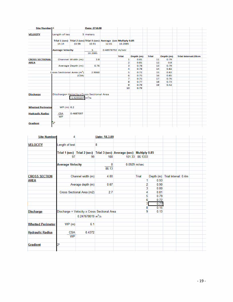
Site Four
Graph Severn: Winter Cross Sectional Area
Created by Simon Johnson, 2009
Graph Eight: Summer Cross Sectional Area
Created by Simon Johnson, 2009
Figure Four: Field Sketch
- 18 -
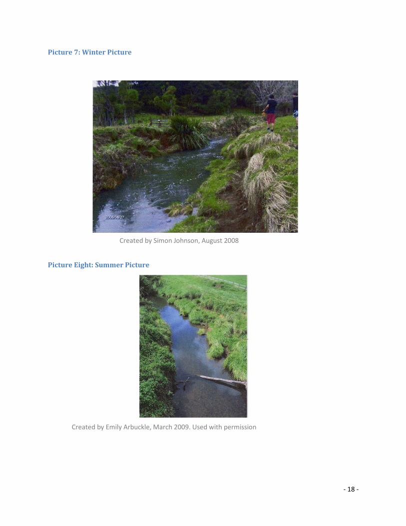
Picture 7: Winter Picture
Created by Simon Johnson, August 2008
Picture Eight: Summer Picture
Created by Emily Arbuckle, March 2009. Used with permission
- 19 -
- 20 -
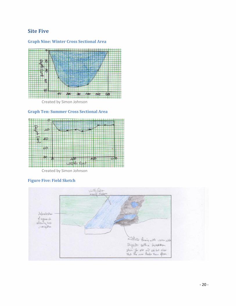
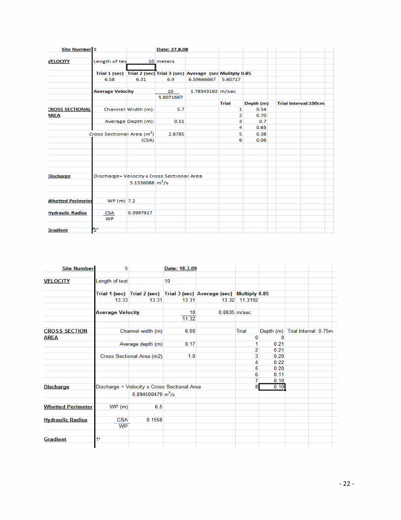
Site Five
Graph Nine: Winter Cross Sectional Area
Created by Simon Johnson
Graph Ten: Summer Cross Sectional Area
Created by Simon Johnson
Figure Five: Field Sketch
- 21 -
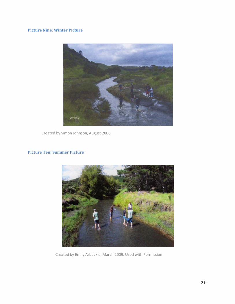
Picture Nine: Winter Picture
Created by Simon Johnson, August 2008
Picture Ten: Summer Picture
Created by Emily Arbuckle, March 2009. Used with Permission
- 22 -
- 23 -
Site Six
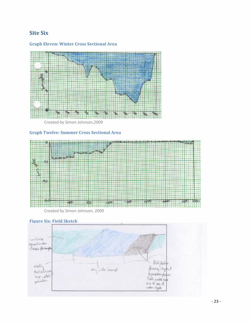
Graph Eleven: Winter Cross Sectional Area
Created by Simon Johnson,2009
Graph Twelve: Summer Cross Sectional Area
Created by Simon Johnson, 2009
Figure Six: Field Sketch
- 24 -
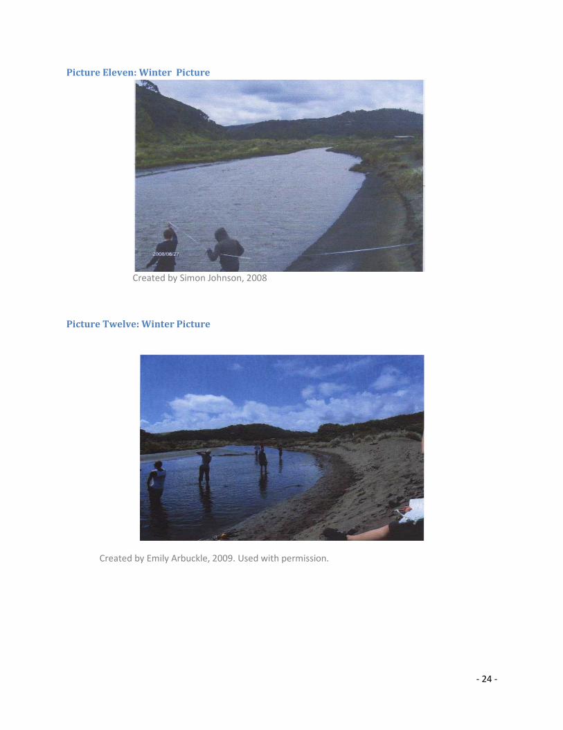
Picture Eleven: Winter Picture
Created by Simon Johnson, 2008
Picture Twelve: Winter Picture
Created by Emily Arbuckle, 2009. Used with permission.
- 25 -
- 26 -
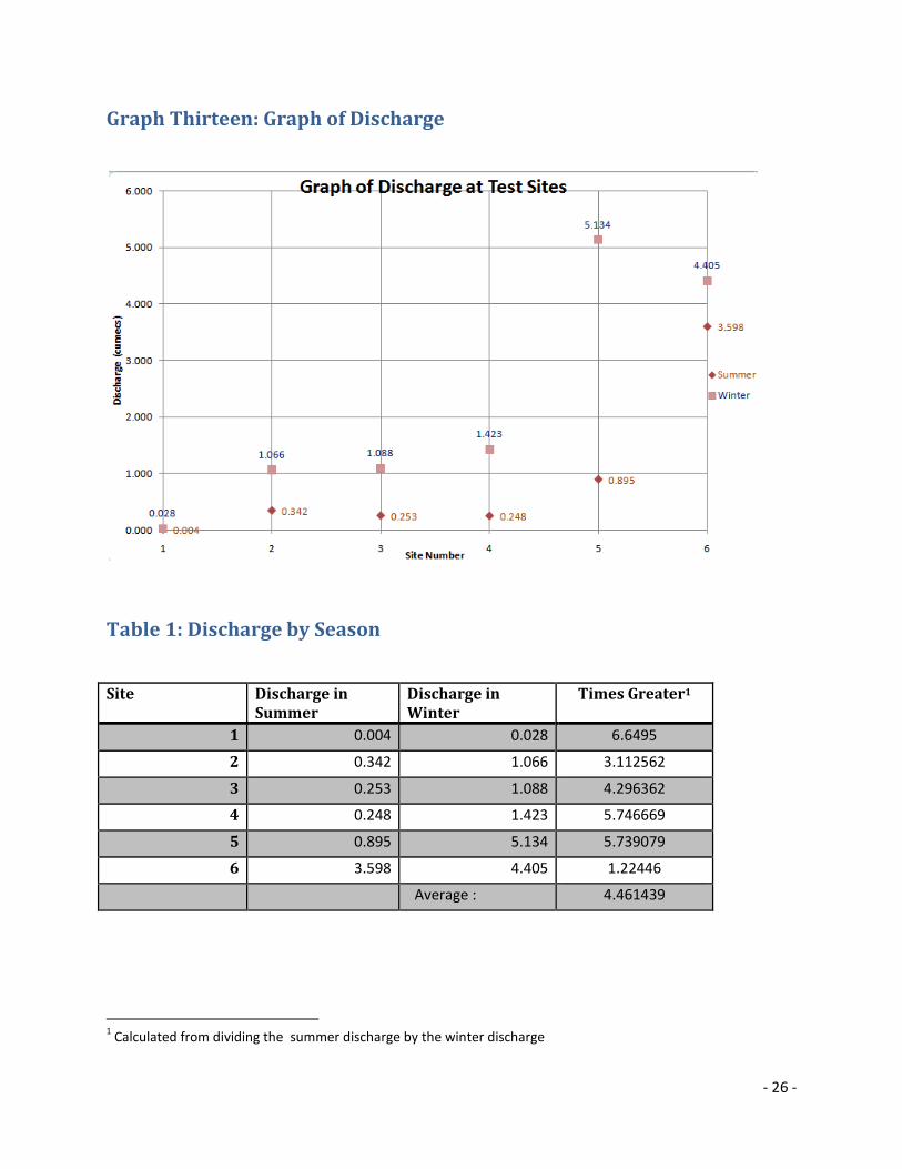
Graph Thirteen: Graph of Discharge
Table 1: Discharge by Season
Site Discharge in
Summer
Discharge in
Winter
Times Greater1
1 0.004 0.028 6.6495
2 0.342 1.066 3.112562
3 0.253 1.088 4.296362
4 0.248 1.423 5.746669
5 0.895 5.134 5.739079
6 3.598 4.405 1.22446
Average : 4.461439
1 Calculated from dividing the summer discharge by the winter discharge
- 27 -
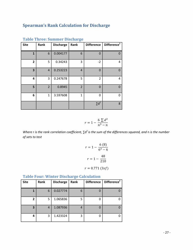
Spearman’s Rank Calculation for Discharge
Table Three: Summer Discharge
Site Rank Discharge Rank Difference Difference2
1 6 0.004177 6 0 0
2 5 0.34243 3 -2 4
3 4 0.253223 4 0 0
4 3 0.247678 5 2 4
5 2 0.8945 2 0 0
6 1 3.597608 1 0 0
∑d2 8
� � 1 � 6 ∑ �
� �
Where r is the rank correlation coefficient, ∑d2
is the sum of the differences squared, and n is the number
of sets to test
� � 1 � 6 �8�
6� � 6
� � 1 � 48
210
� � 0.771 �3���
Table Four: Winter Discharge Calculation
Site Rank Discharge Rank Difference Difference2
1 6 0.027774 6 0 0
2 5 1.065836 5 0 0
3 4 1.087936 4 0 0
4 3 1.423324 3 0 0
- 28 -
5 2 5.133609 1 -1 1
6 1 4.405128 2 1 1
∑d2 2
� � 1 � 6 ∑ �
� �
Where r is the rank correlation coefficient, ∑d2
is the sum of the differences squared, and n is the number
of sets to test
� � 1 � 6 �2�
6� � 6
� � 1 � 12
210
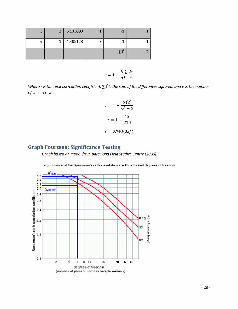
� � 0.943�3���
Graph Fourteen: Significance Testing
Graph based on model from Barcelona Field Studies Centre (2009)
- 29 -
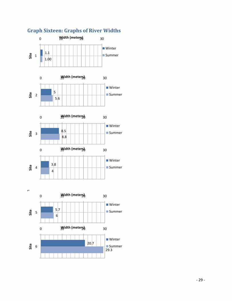
Graph Sixteen: Graphs of River Widths
,.
1.1
1.00
0 10 20 30
1
Width (meters)
Sit
e
Winter
Summer
5
5.6
0 10 20 30
2
Width (meters)
Sit
e
Winter
Summer
8.5
8.8
0 10 20 30
3
Width (meters)
Sit
e
Winter
Summer
3.8
4
0 10 20 30
4
Width (meters)
Sit
e
Winter
Summer
5.7
6
0 10 20 30
5
Width (meters)
Sit
e
Winter
Summer
20.7
29.3
0 10 20 30
6
Width (meters)
Sit
e
Winter
Summer
- 30 -
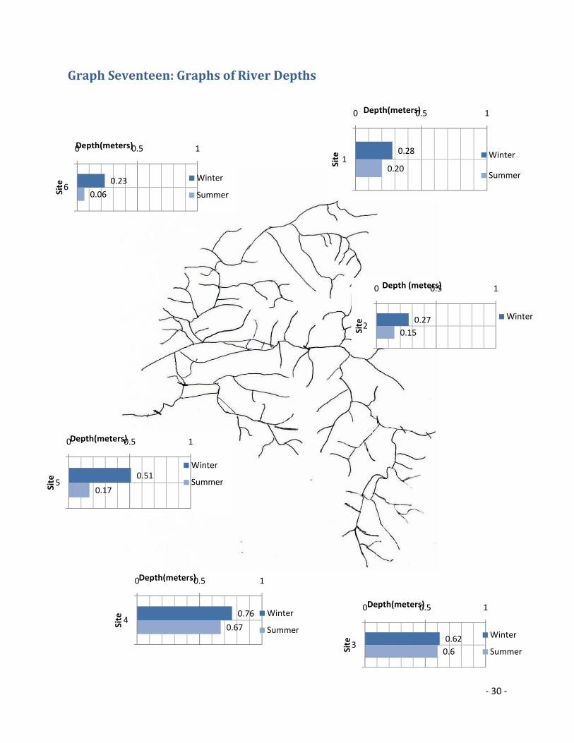
Graph Seventeen: Graphs of River Depths
0.51
0.17
0 0.5 1
5
Depth(meters)
Sit
e
Winter
Summer
0.23
0.06
0 0.5 1
6
Depth(meters)
Sit
e Winter
Summer
0.76
0.67
0 0.5 1
4
Depth(meters)
Sit
e Winter
Summer
0.28
0.20
0 0.5 1
1
Depth(meters)
Sit
e Winter
Summer
0.27
0.15
0 0.5 1
2
Depth (meters)
Sit
e
Winter
0.62
0.6
0 0.5 1
3
Depth(meters)
Sit
e
Winter
Summer
- 31 -
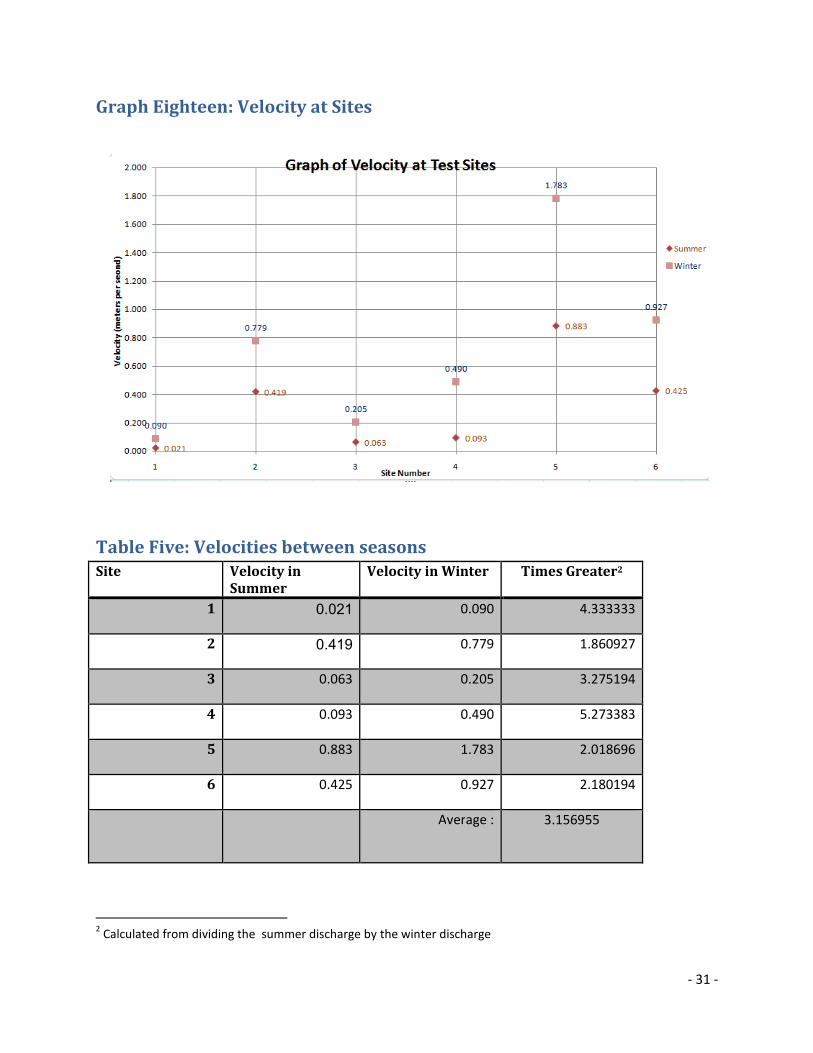
Graph Eighteen: Velocity at Sites
Table Five: Velocities between seasons
Site Velocity in
Summer
Velocity in Winter Times Greater2
1 0.021 0.090 4.333333
2 0.419 0.779 1.860927
3 0.063 0.205 3.275194
4 0.093 0.490 5.273383
5 0.883 1.783 2.018696
6 0.425 0.927 2.180194
Average :
3.156955
2 Calculated from dividing the summer discharge by the winter discharge
- 32 -
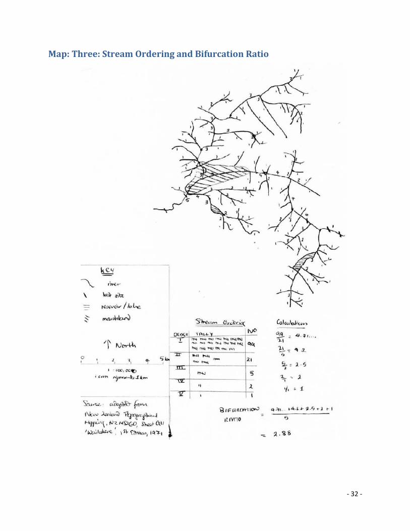
Map: Three: Stream Ordering and Bifurcation Ratio
- 33 -
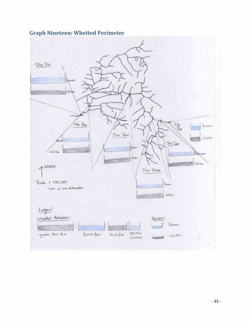
Graph Nineteen: Whetted Perimeter
- 34 -
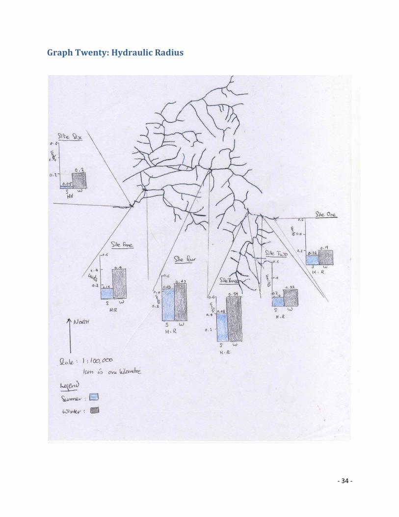
Graph Twenty: Hydraulic Radius
- 35 -
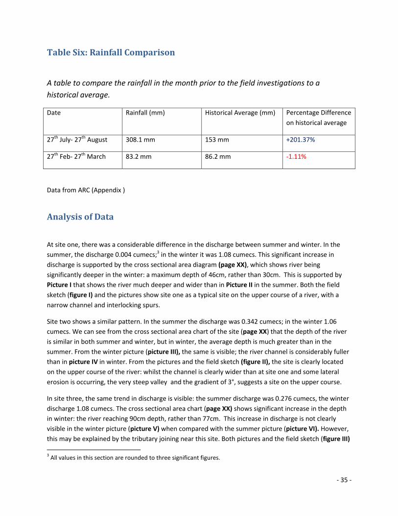
Table Six: Rainfall Comparison
A table to compare the rainfall in the month prior to the field investigations to a
historical average.
Date Rainfall (mm) Historical Average (mm) Percentage Difference
on historical average
27th
July- 27th
August 308.1 mm 153 mm +201.37%
27th
Feb- 27th
March 83.2 mm 86.2 mm -1.11%
Data from ARC (Appendix )
Analysis of Data
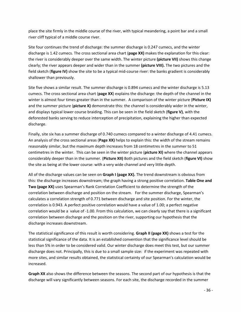
At site one, there was a considerable difference in the discharge between summer and winter. In the
summer, the discharge 0.004 cumecs;3 in the winter it was 1.08 cumecs. This significant increase in
discharge is supported by the cross sectional area diagram (page XX), which shows river being
significantly deeper in the winter: a maximum depth of 46cm, rather than 30cm. This is supported by
Picture I that shows the river much deeper and wider than in Picture II in the summer. Both the field
sketch (figure I) and the pictures show site one as a typical site on the upper course of a river, with a
narrow channel and interlocking spurs.
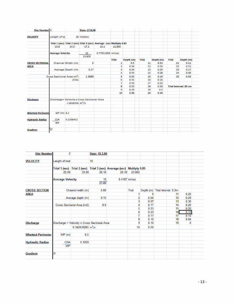
Site two shows a similar pattern. In the summer the discharge was 0.342 cumecs; in the winter 1.06
cumecs. We can see from the cross sectional area chart of the site (page XX) that the depth of the river
is similar in both summer and winter, but in winter, the average depth is much greater than in the
summer. From the winter picture (picture III), the same is visible; the river channel is considerably fuller
than in picture IV in winter. From the pictures and the field sketch (figure II), the site is clearly located
on the upper course of the river: whilst the channel is clearly wider than at site one and some lateral
erosion is occurring, the very steep valley and the gradient of 3°, suggests a site on the upper course.
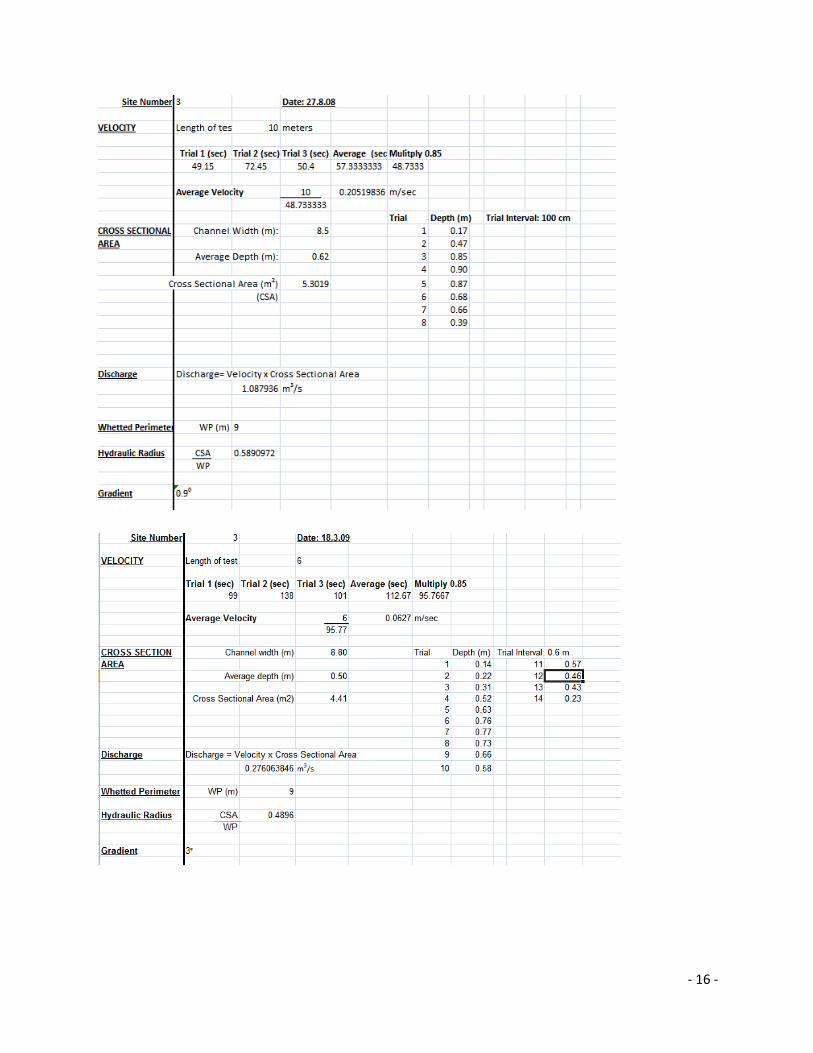
In site three, the same trend in discharge is visible: the summer discharge was 0.276 cumecs, the winter
discharge 1.08 cumecs. The cross sectional area chart (page XX) shows significant increase in the depth
in winter: the river reaching 90cm depth, rather than 77cm. This increase in discharge is not clearly
visible in the winter picture (picture V) when compared with the summer picture (picture VI). However,
this may be explained by the tributary joining near this site. Both pictures and the field sketch (figure III)
3 All values in this section are rounded to three significant figures.
- 36 -
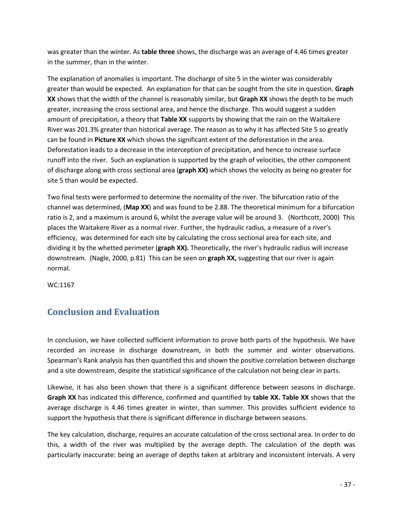
place the site firmly in the middle course of the river, with typical meandering, a point bar and a small
river cliff typical of a middle course river.
Site four continues the trend of discharge: the summer discharge is 0.247 cumecs, and the winter
discharge is 1.42 cumecs. The cross sectional area chart (page XX) makes the explanation for this clear:
the river is considerably deeper over the same width. The winter picture (picture VII) shows this change
clearly; the river appears deeper and wider than in the summer (picture VIII). The two pictures and the
field sketch (figure IV) show the site to be a typical mid-course river: the banks gradient is considerably
shallower than previously.
Site five shows a similar result. The summer discharge is 0.894 cumecs and the winter discharge is 5.13
cumecs. The cross sectional area chart (page XX) explains the discharge: the depth of the channel in the
winter is almost four times greater than in the summer. A comparison of the winter picture (Picture IX)
and the summer picture (picture X) demonstrate this: the channel is considerably wider in the winter,
and displays typical lower course braiding. This can be seen in the field sketch (figure V), with the
deforested banks serving to reduce interception of precipitation, explaining the higher than expected
discharge.
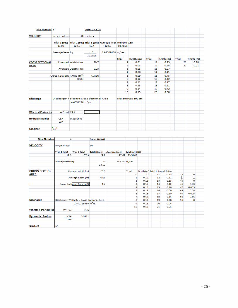
Finally, site six has a summer discharge of 0.740 cumecs compared to a winter discharge of 4.41 cumecs.
An analysis of the cross sectional areas (Page XX) helps to explain this: the width of the stream remains
reasonably similar, but the maximum depth increases from 18 centimetres in the summer to 51
centimetres in the winter. This can be seen in the winter picture (picture XI) where the channel appears
considerably deeper than in the summer. (Picture XII) Both pictures and the field sketch (figure VI) show
the site as being at the lower course: with a very wide channel and very little depth.
All of the discharge values can be seen on Graph I (page XX). The trend downstream is obvious from
this: the discharge increases downstream; the graph having a strong positive correlation. Table One and
Two (page XX) uses Spearman’s Rank Correlation Coefficient to determine the strength of the
correlation between discharge and position on the stream. For the summer discharge, Spearman’s
calculates a correlation strength of 0.771 between discharge and site position. For the winter, the
correlation is 0.943. A perfect positive correlation would have a value of 1.00; a perfect negative
correlation would be a value of -1.00. From this calculation, we can clearly say that there is a significant
correlation between discharge and the position on the river, supporting our hypothesis that the
discharge increases downstream.
The statistical significance of this result is worth considering. Graph II (page XX) shows a test for the
statistical significance of the data. It is an established convention that the significance level should be
less than 5% in order to be considered valid. Our winter discharge does meet this test, but our summer
discharge does not. Principally, this is due to a small sample size: if the experiment was repeated with
more sites, and similar results obtained, the statistical certainty of our Spearman’s calculation would be
increased.
Graph XX also shows the difference between the seasons. The second part of our hypothesis is that the
discharge will vary significantly between seasons. For each site, the discharge recorded in the summer
- 37 -
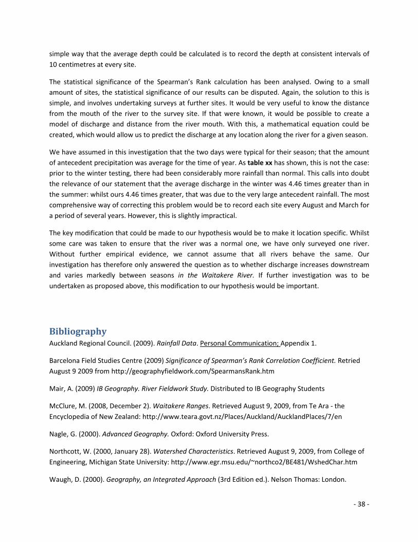
was greater than the winter. As table three shows, the discharge was an average of 4.46 times greater
in the summer, than in the winter.
The explanation of anomalies is important. The discharge of site 5 in the winter was considerably
greater than would be expected. An explanation for that can be sought from the site in question. Graph
XX shows that the width of the channel is reasonably similar, but Graph XX shows the depth to be much
greater, increasing the cross sectional area, and hence the discharge. This would suggest a sudden
amount of precipitation, a theory that Table XX supports by showing that the rain on the Waitakere
River was 201.3% greater than historical average. The reason as to why it has affected Site 5 so greatly
can be found in Picture XX which shows the significant extent of the deforestation in the area.
Deforestation leads to a decrease in the interception of precipitation, and hence to increase surface
runoff into the river. Such an explanation is supported by the graph of velocities, the other component
of discharge along with cross sectional area (graph XX) which shows the velocity as being no greater for
site 5 than would be expected.
Two final tests were performed to determine the normality of the river. The bifurcation ratio of the
channel was determined, (Map XX) and was found to be 2.88. The theoretical minimum for a bifurcation
ratio is 2, and a maximum is around 6, whilst the average value will be around 3. (Northcott, 2000) This
places the Waitakere River as a normal river. Further, the hydraulic radius, a measure of a river’s
efficiency, was determined for each site by calculating the cross sectional area for each site, and
dividing it by the whetted perimeter (graph XX). Theoretically, the river’s hydraulic radius will increase
downstream. (Nagle, 2000, p.81) This can be seen on graph XX, suggesting that our river is again
normal.
WC:1167
Conclusion and Evaluation
In conclusion, we have collected sufficient information to prove both parts of the hypothesis. We have
recorded an increase in discharge downstream, in both the summer and winter observations.
Spearman’s Rank analysis has then quantified this and shown the positive correlation between discharge
and a site downstream, despite the statistical significance of the calculation not being clear in parts.
Likewise, it has also been shown that there is a significant difference between seasons in discharge.
Graph XX has indicated this difference, confirmed and quantified by table XX. Table XX shows that the
average discharge is 4.46 times greater in winter, than summer. This provides sufficient evidence to
support the hypothesis that there is significant difference in discharge between seasons.
The key calculation, discharge, requires an accurate calculation of the cross sectional area. In order to do
this, a width of the river was multiplied by the average depth. The calculation of the depth was
particularly inaccurate: being an average of depths taken at arbitrary and inconsistent intervals. A very
- 38 -
simple way that the average depth could be calculated is to record the depth at consistent intervals of
10 centimetres at every site.
The statistical significance of the Spearman’s Rank calculation has been analysed. Owing to a small
amount of sites, the statistical significance of our results can be disputed. Again, the solution to this is
simple, and involves undertaking surveys at further sites. It would be very useful to know the distance
from the mouth of the river to the survey site. If that were known, it would be possible to create a
model of discharge and distance from the river mouth. With this, a mathematical equation could be
created, which would allow us to predict the discharge at any location along the river for a given season.
We have assumed in this investigation that the two days were typical for their season; that the amount
of antecedent precipitation was average for the time of year. As table xx has shown, this is not the case:
prior to the winter testing, there had been considerably more rainfall than normal. This calls into doubt
the relevance of our statement that the average discharge in the winter was 4.46 times greater than in
the summer: whilst ours 4.46 times greater, that was due to the very large antecedent rainfall. The most
comprehensive way of correcting this problem would be to record each site every August and March for
a period of several years. However, this is slightly impractical.
The key modification that could be made to our hypothesis would be to make it location specific. Whilst
some care was taken to ensure that the river was a normal one, we have only surveyed one river.
Without further empirical evidence, we cannot assume that all rivers behave the same. Our
investigation has therefore only answered the question as to whether discharge increases downstream
and varies markedly between seasons in the Waitakere River. If further investigation was to be
undertaken as proposed above, this modification to our hypothesis would be important.
Bibliography
Auckland Regional Council. (2009). Rainfall Data. Personal Communication; Appendix 1.
Barcelona Field Studies Centre (2009) Significance of Spearman’s Rank Correlation Coefficient. Retried
August 9 2009 from http://geographyfieldwork.com/SpearmansRank.htm
Mair, A. (2009) IB Geography. River Fieldwork Study. Distributed to IB Geography Students
McClure, M. (2008, December 2). Waitakere Ranges. Retrieved August 9, 2009, from Te Ara - the
Encyclopedia of New Zealand: http://www.teara.govt.nz/Places/Auckland/AucklandPlaces/7/en
Nagle, G. (2000). Advanced Geography. Oxford: Oxford University Press.
Northcott, W. (2000, January 28). Watershed Characteristics. Retrieved August 9, 2009, from College of
Engineering, Michigan State University: http://www.egr.msu.edu/~northco2/BE481/WshedChar.htm
Waugh, D. (2000). Geography, an Integrated Approach (3rd Edition ed.). Nelson Thomas: London.

- 39 -