THE WAV EFIELD OF ACOUSTIC LOGGING IN A … Wavefield...5 6 7 8 9 10 11 12 13 14 15 16 17 18 19 20 21 22 23 24 25 26 27 28 29 30 31 32 33 34 35 36 37 38 39 40 41 42 43 44 45 46 47

THE WAVEFIELD OF ACOUSTIC LOGGING IN A CASED-HOLE

WITH A SINGE CASING - PART I: A MONOPOLE TOOL

Journal: Geophysical Journal International

Manuscript ID Draft

Manuscript Type: Research Paper

Date Submitted by the Author: n/a

Complete List of Authors: Wang, Hua; Massachusetts Institute of Technology, Department of Earth, Atmospheric and Planetary Sciences Fehler, Michael; Massachusetts Institute of Technology, Dept. of Earth, Atmospheric, and Planetary Sciences

Keywords: Downhole methods < GEOPHYSICAL METHODS, Numerical modelling < GEOPHYSICAL METHODS, Acoustic properties < SEISMOLOGY, Guided

waves < SEISMOLOGY, Wave propagation < SEISMOLOGY

Geophysical Journal International

1

THE WAVEFIELD OF ACOUSTIC LOGGING IN A

CASED-HOLE WITH A SINGE CASING - PART I: A

MONOPOLE TOOL

Hua Wang*, Mike Fehler, Earth Resources Lab, MIT

*Corresponding author: [email protected]

Page 1 of 40 Geophysical Journal International

123456789101112131415161718192021222324252627282930313233343536373839404142434445464748495051525354555657585960

2

SUMMARY

The bonding of the cement between casing and formation is critical for the

hydraulic isolation of reservoir layers with shallow aquifers, production and

environmental safety, and plug and abandonment issues. Acoustic logging is a

very good tool for evaluating the condition of the bond between different

interfaces. Our understanding of the wavefields in wells with single casing is

still incomplete. We use a 3D Finite Difference (3DFD) method to simulate

monopole wavefields in a singly-cased borehole with different bonding

conditions between the cement and casing and the cement and formation.

Pressure snapshots and waveforms for different models are shown which

allow us to better understand the wave propagation. Modal dispersion curves

for different models and data processing methods such as velocity-time

semblance and dispersion analysis facilitate the identification of propagation

modes in the different models. We find that the P wave is submerged in the

casing modes and the S wave has poor coherency when the cement is replaced

with fluid. The casing modes are strong when cement next to the casing is

partially or fully replaced with fluid. The amplitude of these modes can be

used for determine the bonding condition of the interface between casing and

cement. While the amplitude changing for different fluid thickness is hard to

pick which would result in the ambiguity on interpretation. The casing modes

are different when the cement next to the formation is partially replaced with

fluid, which are the modes propagate in the mixed material of steel pipe and

Page 2 of 40Geophysical Journal International

123456789101112131415161718192021222324252627282930313233343536373839404142434445464748495051525354555657585960

3

cement and the velocities are highly dependent on the cement thickness. It

would highly possibly misjudge cement quality because the amplitudes of

these modes are very small and they propagate with nearly the formation P

velocity. However, it is possible to use the amplitude to estimate the thickness

of the cement sheath because the variation of amplitude with thickness is very

clear. While the Stoneley mode (ST1) propagates in the borehole fluid, a slow

Stoneley mode (ST2) appears in the fluid column outside the casing when

cement is partially or fully replaced with fluid. The velocity of ST2 is

sensitive to the total thickness of the fluid column in the annulus independent

of the location of the fluid in the casing annulus. By combining measurements

of the first arrival amplitude and ST2 velocity, we propose a full waveform

method that can be used to eliminate the ambiguity and improve cement

evaluation compared to the current method that uses only the first arrival.

Keywords: first arrival, tube wave, cement bond evaluation, sonic full waveforms


123456789101112131415161718192021222324252627282930313233343536373839404142434445464748495051525354555657585960

4

INTRODUCTION

The condition of the bond in a cemented cased well is very critical to the

borehole integrity. It affects the production efficiency as well as production

and environmental safety (Lecampion et al., 2011). It is thus essential to

accurately evaluate the material bonding behind casing.

Acoustic logging methods, the most commonly used methods for evaluating

the cement quality which have typically been used during the well

construction, are designed for material evaluation behind single casing strings

(Pardue et al., 1963; Zhang et al., 2011; Wang et al., 2016). In this case, there are

two bonding interfaces, bonding interface I: interface between the casing and

material next to the casing, bonding interface II: interface next to the

formation. The methods for cement bonding evaluation are most often used to

evaluate the bonding condition at these two interfaces.

Currently, the most commonly used method in the industry is cement bond

logging (CBL), in which the attenuation factor is measured from the first

arrival amplitude only, whereas variable density logging (VDL) uses the

amplitude of the full waveform (Walker, 1968). These methods are based on the

relationship between the amplitude of the casing wave and the fluid column thickness

(e.g. Jutten & Corrigall, 1989; Liu et al., 2011; Tang et al., 2016), and on the arrival

time (Zhang et al., 2013) of the first arrival. The attenuation value is also inversely

proportional to the cement coverage in azimuth. Measurements made on the first


123456789101112131415161718192021222324252627282930313233343536373839404142434445464748495051525354555657585960

5

arrival can be ambiguous because of the small amplitude of the first arrival. In

particular, if the interface I is not cemented, the CBL/VDL cannot tell the bonding

condition of interface II. Therefore it is beneficial to study the wavefields in the

single casing situation to determine the possibility of evaluating the bonding

condition by using full waveforms rather the currently used first arrival

method. Although a number of studies have been conducted for single casing

strings (e.g. Tubman et. al., 1984; Zhang et. al., 2013), the understanding of

the wavefields in the single casing model is still incomplete. In this paper, we

use a 3D finite difference method (3DFD) to simulate the monopole wavefield

in single casing models with different bonding conditions. We investigate the

different modes propagating in the borehole by analysis of the simulated 3D

wavefield records. By using data processing methods we attempt to

understand if we can identify a relationship between fundamental mode

propagation and the condition of the cement bonds.

METHOD

Although analytical or semi-analytical methods can get accurate solutions for

simple models, they cannot get the solutions for models with complicated

geometries. For complex models we must appeal to numerical methods such

as 3DFD. We use the 3DFD code that has previously been used by Wang et

al. (2015) to simulate wave propagation in boreholes with a single casing

string. The code uses a staggered grid and is second order in both space and


123456789101112131415161718192021222324252627282930313233343536373839404142434445464748495051525354555657585960

6

time that allows correct results even in situations that have high impedance

contrast between fluid and solid. Prior to using our 3DFD code, we must

confirm its reliability for modeling situations where the steel casing is present

in the model. A singly-cased borehole model consists of multiple concentric

cylinders. The innermost cylinder is the borehole fluid and second is the steel

pipe (or casing). The outermost cylinder is the formation (e.g. sandstone in

Table 1). The material filling the cylinder between the steel pipe and

formation is cement. The cement may be partially or fully replaced with fluid.

Table 1 lists the geometries and elastic parameters of an example fully

cemented cased hole (shown in Fig. 1). In this study, we only change the

geometry and filling material of the cement cylinder to investigate the effect

of different bonding conditions on full waveforms.

For the code validation, we investigate the case of sonic logging in a hole in

which the cement outside the steel casing is completely replaced by fluid. A

ring source is approximated by 36 several point sources embedded on the

outer boundary of the casing. Although the source loading is different from

the sonic logging in cased hole, which is a centralized source in the inner

fluid, we choose this model because we can easily use the Discrete

Wavenumber integration method (DWM, Byun & Toksöz, 2003) develope for

an ALWD model (Wang et al., 2015). We use a 10 kHz Ricker wavelet

source, which covers the frequency band of the most common sonic logging

tools.


123456789101112131415161718192021222324252627282930313233343536373839404142434445464748495051525354555657585960

7

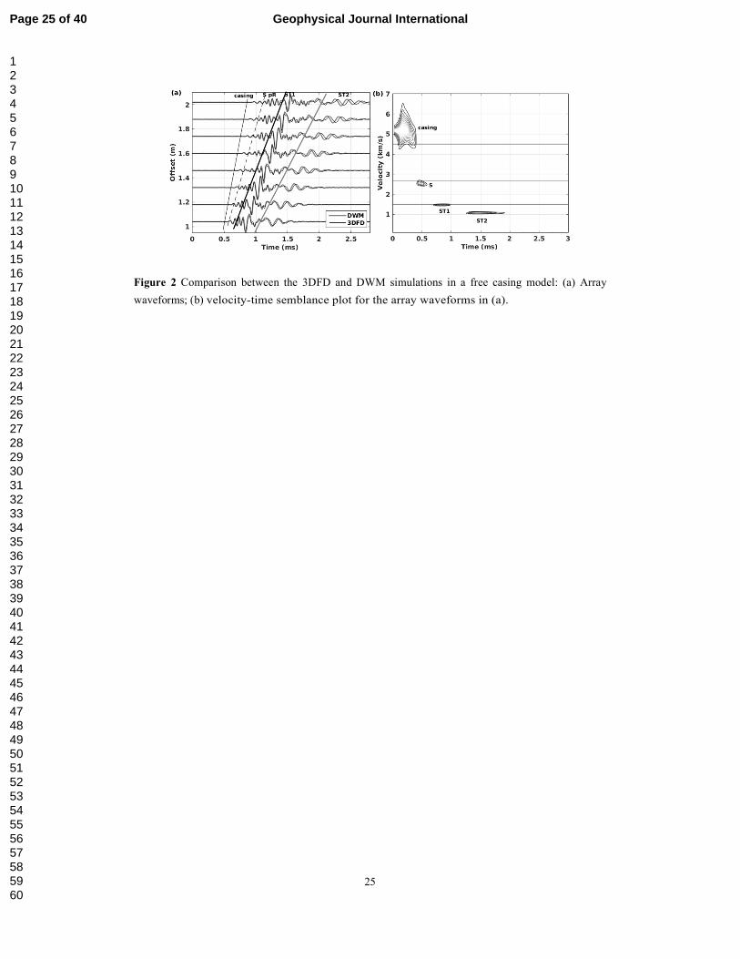
Fig. 2 shows the simulations obtained using both 3DFD and DWM. The grid

sizes of 1 mm in x and y, and 2 mm in z directions are used in the 3DFD code.

The array waveforms (Fig. 2a) show a nearly perfect match between the FD

and DWM excepting the difference appears in the later part of the waveform

(after 1 ms) due to the numerical dispersion of FD in the z direction. This

late-arriving mode corresponds to the ST (Stoneley) wave propagating in the

fluid column between casing and formation (marked as ST2). The casing mode,

S and pR (pseudo Rayleigh), and ST1 (Stoneley in the fluid column inside the steel

pipe) waves can be easily found with different lines marked according to their arrival

times and also in the velocity-time semblance plot (Fig. 2b).

NUMERICAL SIMULATIONS

Here we use our 3DFD simulator to investigate the full waveforms and wave

propagation characteristics by examining wavefield snapshots for three different

models: (1) casing immersed in fluid, (2) free casing in a borehole, and (3) perfect

cement bonding between casing and formation.

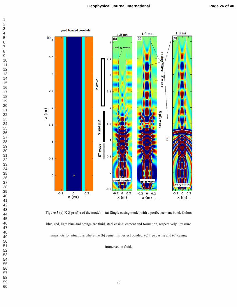
Fig. 3a shows side views of the borehole model with good cement between casing and

formation. For the model with the casing immersed in a fluid, the cement and

formation are completely replaced with fluid. We use this model to understand the

modes propagating on the pipe and the wavefield can also help the understanding of

the application not only the single cased-hole but also underwater cables and oil and

chemical pipelines. For the free casing model, the cement is replaced with fluid. In the


123456789101112131415161718192021222324252627282930313233343536373839404142434445464748495051525354555657585960

8

simulations, the effect of the tool is ignored and a centralized point source with a 10

kHz Ricker wavelet is used. The pressure snapshots at 1.0 ms on a x-z profile are

shown in Figs. 3b (good bond), 3c (free casing) and 3d (casing immersed in fluid). Fig.

3d can help us understand the modes in the casing.

As has been shown in nondestructive testing, there are three types of guided wave in

pipes: L (longitude), F (flexural), and T (torsional) modes (Cawley et al., 2002). T

modes are associated with pipe rotation and would be found in the drilling pipe.

During the acoustic logging in the cased hole, L modes are monopole modes in the

casing which are similar as the extensional modes in the collar in acoustic

logging-while-drilling. F modes are dipole and quadrupole (even higher) modes in the

pipe (similar as the flexural, screw modes on collar in acoustic logging-while-drilling).

Here we find casing modes (L modes) at offsets of about 1.5 to 4 m while the ST

wave follows and both modes leak into both sides of the casing as leaky modes that

can be seen in Fig. 3d. We use a dense receiver array with a 0.1 m interval to record

the waveforms from the source position to the top of model along the z axis to

understand the wave modes (as shown in Fig. 4a). We find three visible modes as

marked with lines. Comparing the extracted frequency-velocity semblance plot (Wang

et al., 2015) from the array waveforms with the modal dispersion curves (solid lines)

(Tubman et al., 1984; Zhang et al., 2016) in Fig. 4b, we find that the modes are the L

casing modes (L1 to L4), ST1 and an additional ST2 (slow ST in Plona et al., 1992).

Other modes including P, S, and pR (pseudo Rayleigh) modes are marked in


123456789101112131415161718192021222324252627282930313233343536373839404142434445464748495051525354555657585960

9

Figs. 3b and 3c. Although the wave front of the casing modes propagate as the

fastest ones in the pressure snapshots, the modes do not leak and are trapped

in the casing when the casing is well cemented, which makes them invisible

both in the borehole and formation (as shown in Fig. 3b). The formation P and

S waves are detected by a centralized array receiver. However, the casing

mode leaks into the fluid when the coupling is not good as seen in the free

casing model shown in Fig. 3c. In this situation, the first arrival in the

borehole is the strong leaky casing mode and the formation P wave is

submerged.

Fig. 5 shows the array waveforms obtained from a centralized receiver in the

models (displayed the same way as Fig. 4a) and the related velocity analysis

in the time (Kimball & Marzetta, 1986) and frequency domains. Figs. 5a to 5c

are for the well cemented cased hole. We see the waveforms having a time

sequence of P, S, pR, ST and pR modes in Fig. 5a. The waveforms at offsets

of 3 m to 3.7 m (interval of 0.1 m) are used for calculating velocity-time

semblance (Fig. 5b) and dispersion (Fig. 5c). From the plots, we discern the P,

S, multiple orders of pR, and ST modes, respectively. The waveforms are very

different when the cement is completely replaced with fluid and the wave

modes in time sequence (Fig. 5d) are casing, S that is not very coherent

(Paillet & Cheng, 1991), ST, and the strongly dispersive pR (additional ST

from the fluid between casing and formation being buried within the

waveforms). The velocity plots in Figs. 5e and 5f also show those modes. It is


123456789101112131415161718192021222324252627282930313233343536373839404142434445464748495051525354555657585960

10

obvious that there are two ST modes in Fig. 5f corresponding to a ST inside

the casing with a higher velocity and an additional ST in the fluid between

casing and formation with a slower velocity.

The wavefield for the free casing model shows a very interesting additional

ST mode (Similar phoneme could found in Marzetta & Schoenberg(1985) and

Daley et al.(2013)) that is not present when there is good cement between the

casing and formation. However, this additional mode is not very visible when

the source frequency around 10 kHz. To investigate the influence of the

source frequency on the amplitudes of different modes in the free casing

model, we plot the waveforms at different source frequencies in Fig. 6. Modes

are marked in the plots by the arrival times. It is easy to find the relationship

between the source frequency and the amplitude of modes. The casing mode

is weak below 3 kHz. We get much more obvious ST modes at low frequency.

However, if the frequency is too low, we cannot identify ST2 from the

waveforms. According to Figs. 5f and 6, we find that if the source frequency

is set at around 6 kHz, it is easy to identify the obvious ST modes.

PARTIALLY BONDED MODELS

Based on the dispersion curves and waveforms from the free casing model, we

propose that the newly identified ST2 mode would be an indicator of the

cement bonding condition. In the following sections, we discuss the


123456789101112131415161718192021222324252627282930313233343536373839404142434445464748495051525354555657585960

11

wavefields of the partially cemented models to determine the possibility of

evaluating the bonding condition by using full waveforms rather than the

current method based on the first arrival (e.g. Walker, 1968; Zhang et al.,

2011).

By investigating the detail of the wavefields for models with different

thicknesses of fluid and cement, we hope to get a direct method to determine

the bonding condition including that between the outer casing interface and

the formation by using data acquired by a commonly used array acoustic

logging tool with a source having sonic frequencies (e.g. Zhang, et al., 2011).

Fluid between steel casing and cement

We first consider models in which some of the cement next to the casing (bonding

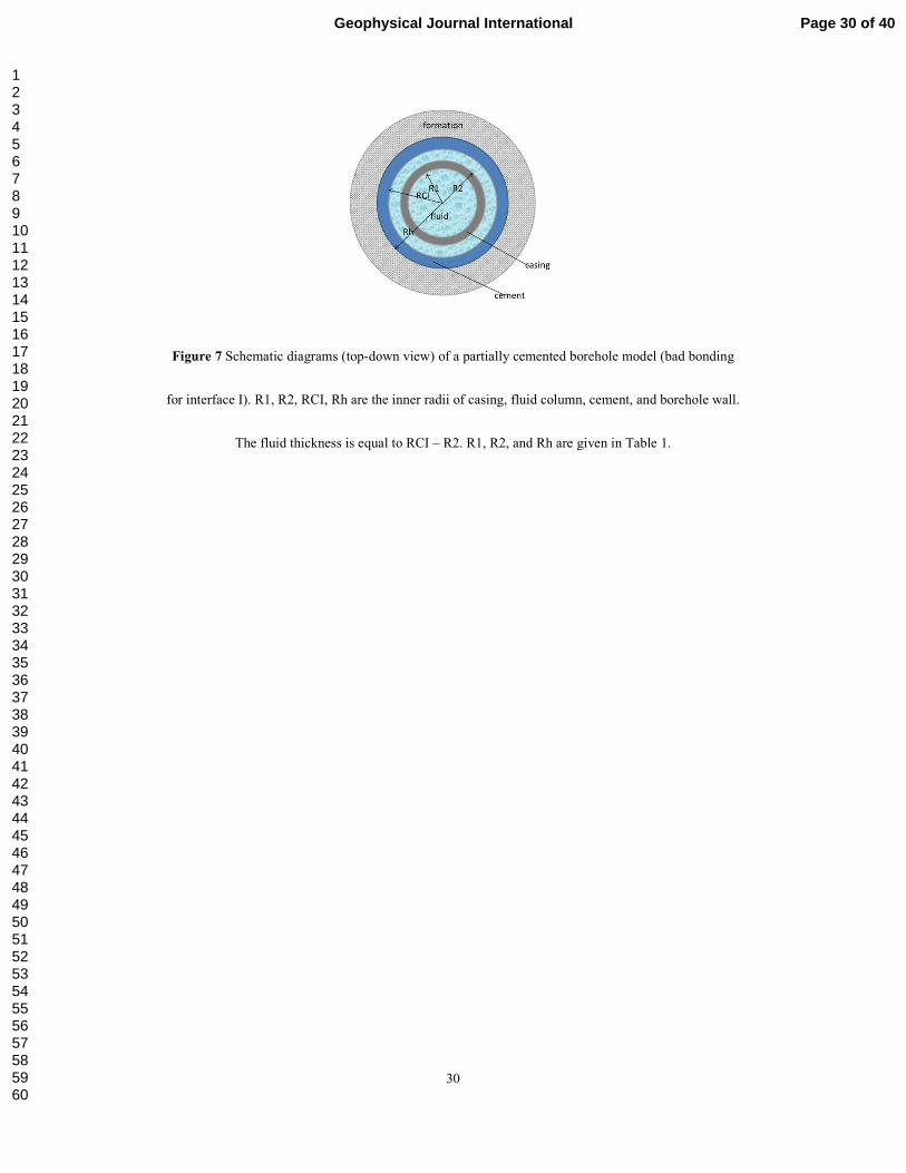
interface I) is replaced with fluid. Fig. 7 shows a schematic diagram (top-down view)

of a partially cemented borehole model. R1, R2, RCI, and Rh are the inner radii of

casing, fluid column, cement, and borehole wall. The fluid thickness is equal to RCI –

R2. With R2 of 122 mm (Table 1), we investigate the wavefields in the models with

RCI of 122 mm, 122.5 mm, 123 mm, 124 mm, 126 mm, 130 mm, 138 mm, 154 mm,

162 mm and 170 mm, which are corresponding to the models with the fluid thickness

of 0 mm (fully cemented), 0.5 mm, 1 mm, 2 mm, 4 mm, 8 mm, 16 mm, 32 mm, 40

mm, and 48 mm (no cement) next to the casing.

We calculate the modal dispersion curves for the models and find that the ST2 and

casing modes vary with the fluid thickness (as shown in Fig. 8) while other modes


123456789101112131415161718192021222324252627282930313233343536373839404142434445464748495051525354555657585960

12

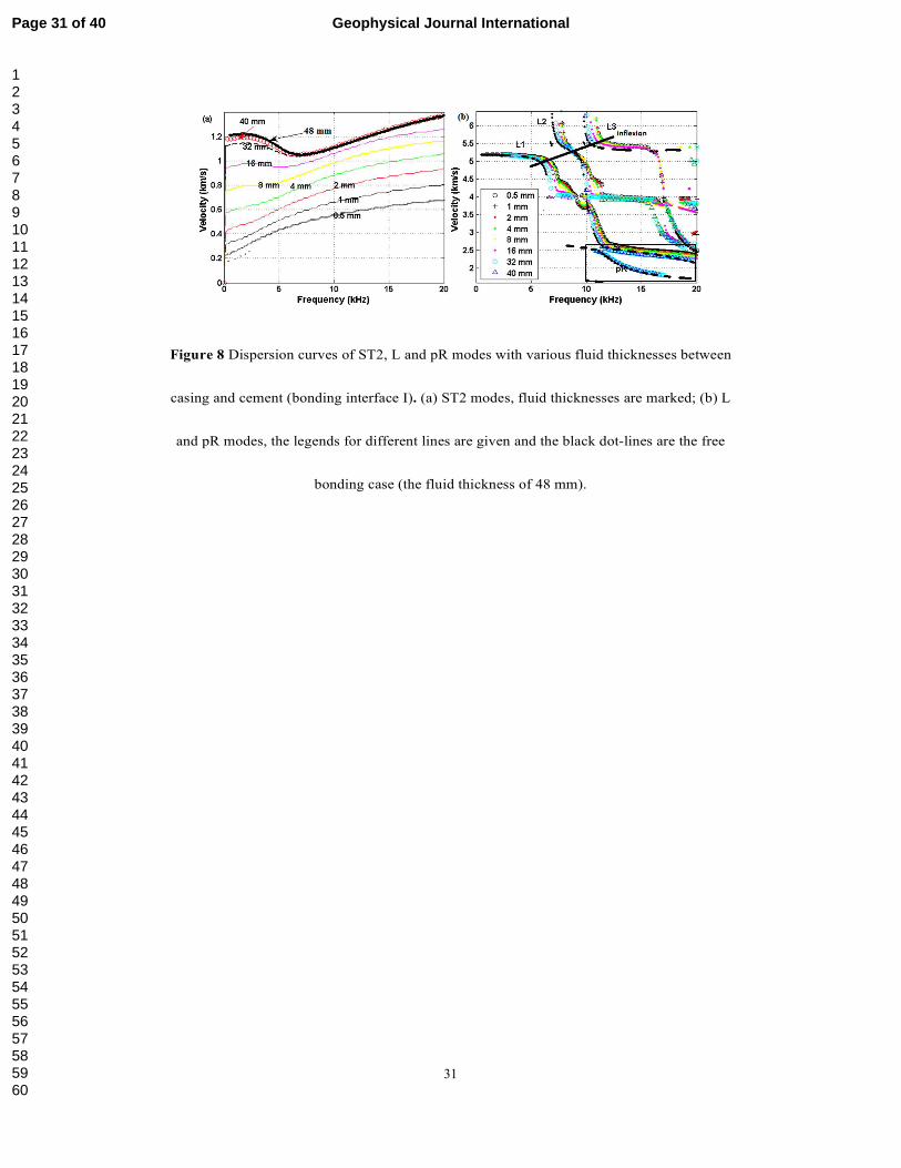
such as ST1 and pR have no change. Fig. 8a shows the dispersion curves for ST2 with

various fluid thicknesses. We find the ST2 mode is very sensitive to the fluid

thickness. The velocity of ST2 increases with the fluid thickness. This means that the

velocity could be a good indicator for cement bond evaluation.

There is very small difference in velocity of the L modes with fluid thicknesses (as

shown in Fig. 8b). The black dotted lines, denoting the modes in the free casing model

(the fluid thickness of 48 mm), are almost the same as the modes in the cases with

partial cement except at the lower frequencies at the inflection points (marked with a

solid line) for different L modes.

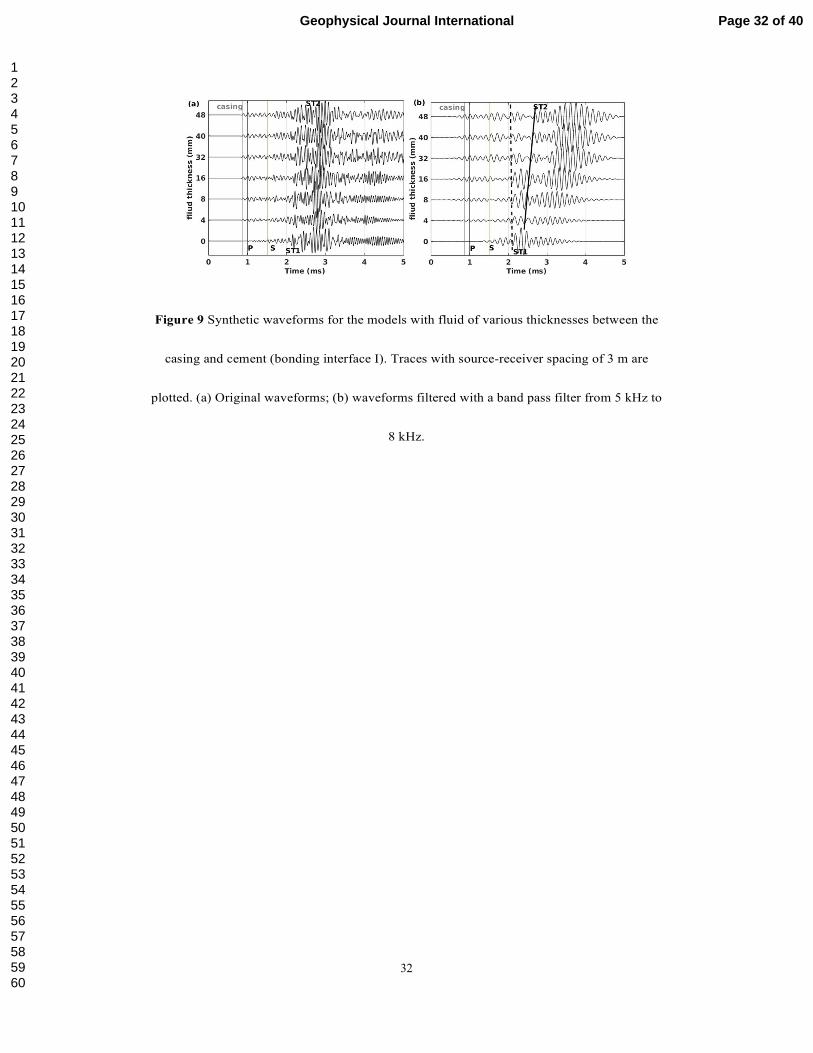
We simulate the full waveforms for most of the models (the fluid thickness of 0 mm,

4 mm, 8 mm, 16 mm, 32 mm, 40 mm, and 48 mm) as shown in Fig. 9 ( traces for

source-receiver spacing of 3 m are shown). In Fig. 9a, we see the clear casing mode as

the first arrival when the cement is partially replaced with fluid. Walker (1968) was

the first to give the relationship between the amplitude of the casing modes and the

thicknesses of cement sheath. The current methods for cement evaluation are mostly

based on his relationship by using the amplitude of the casing modes. However, the

small dependence of the amplitude of the first arrival with fluid thickness, shown in

Fig. 9a, challenges the tool design and data processing. The added uncertainty from

working in down-hole environment contributes to the difficulty. The P wave is

submerged in the casing modes and cannot be discerned which is similar to the case


123456789101112131415161718192021222324252627282930313233343536373839404142434445464748495051525354555657585960

13

of P wave measurements in fast-fast formations in acoustic logging-while-drilling

situations (Wang et al., 2017). The difficult to discern arrival time of S wave make the

velocity measurement difficult when fluid exists next to the casing. The ST1 and ST2

modes are hard to discern due to the strong interference from pR. As we found in

Fig. 6, we get a visible ST2 mode when the source frequency is around 6 kHz.

Fig. 9b shows traces that have been filtered using a 5 kHz to 8 kHz band filter.

It is easy to identify ST1 and ST2 in the waveforms although the ST2 is not

clear when the fluid thickness is 4 mm and 8 mm. The small velocity of ST2

suggests that a tool with a large offset would be helpful to separate the ST1

and ST2 for the small fluid thickness cases. The velocity analyses in time and

frequency domains (based on the filtered data for the case with the fluid

thickness of 16 mm) are given in Fig. 10.

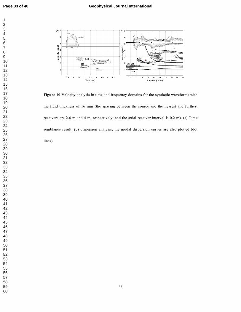
We easily find casing, S and pR, ST1, and ST2 modes from the velocity-time

semblance plot (Fig. 10a), which is similar as Fig. 5e for the free casing

situation. However, the separation between these two modes is larger than the

free casing model due to the slower ST2. In Fig. 10b, we plot the modal

dispersion curves using dotted lines on the dispersion analysis contour plot

which is obtained from the array waveforms. The match between the modal

dispersion curves and dispersion analysis plot for different modes is very good,

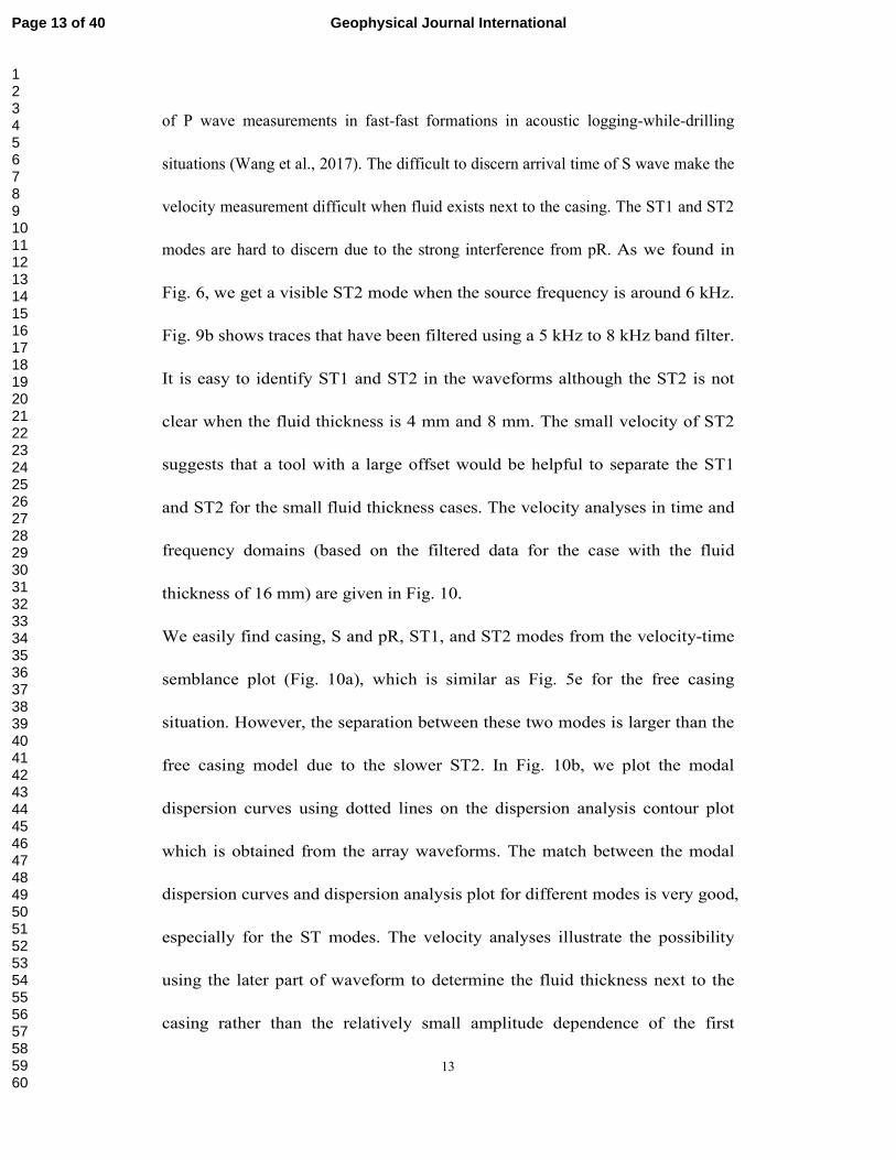
especially for the ST modes. The velocity analyses illustrate the possibility

using the later part of waveform to determine the fluid thickness next to the

casing rather than the relatively small amplitude dependence of the first


123456789101112131415161718192021222324252627282930313233343536373839404142434445464748495051525354555657585960

14

arrival on thickness. If we find casing modes, we can consider the interface

between casing and cement is filled with fluid and then we can use the ST2 to

determine the thickness of the fluid column.

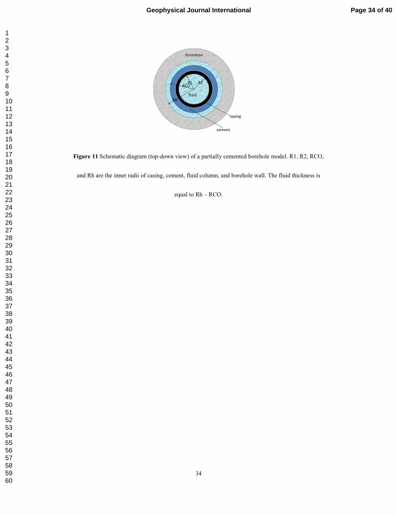
Fluid between cement sheath and formation

It is very critical to evaluate the bonding condition of interface (bonding interface II)

between the cement and formation because it is close to the reservoir or aquifer. Here

we investigate the models with some of the cement in between the casing and

formation being replacing with fluid. Fig. 11 shows a schematic diagram (top-down

view) of a partially cemented borehole model. R1, R2, RCO, and Rh are the inner

radii of casing, cement, fluid column, and borehole wall. The fluid thickness is equal

to Rh – RCO. We investigate the wavefields in the models with RCO of 170 mm,

169.5 mm, 169 mm, 168 mm, 166 mm, 162 mm, 154 mm, 138 mm, 154 mm, 130 mm

and 122 mm, which correspond to models with the fluid thickness of 0 mm (fully

cemented), 0.5 mm, 1 mm, 2 mm, 4 mm, 8 mm, 16 mm, 32 mm, 40 mm, and 48 mm

(no cement) in front of the formation.

We will not display the modal dispersion curves for the models here because the

characteristics are similar to those in Fig. 8 for bonding interface I. There are L, pR,

ST1, and ST2 modes. The only difference is the lower speed of the L modes and the

shifting of the inflection points to lower frequency. Here the L modes propagate in a

mixed material of steel pipe and cement with the slower speeds since they no longer

only propagate in the steel pipe. The cement next to casing enlarges the effective


123456789101112131415161718192021222324252627282930313233343536373839404142434445464748495051525354555657585960

15

radius of the pipe and moves the inflection points to lower frequencies. The trend of

the dispersion curves of these modes is that with more cement, velocity decreases and

the inflection point shifts towards lower frequency. We cannot find any difference in

dispersion for mode ST2 from that shown in Fig. 8a for the corresponding fluid

thickness cases. This suggests that ST2 cannot be used as indicator for the location of

where the fluid column exists. However, at a minimum, we can know whether

interface II is bonded well by using the arrival time and velocity of the L modes

(Zhang et al., 2011). Then we can determine the thickness of the fluid column next to

the formation by using the ST2 mode.

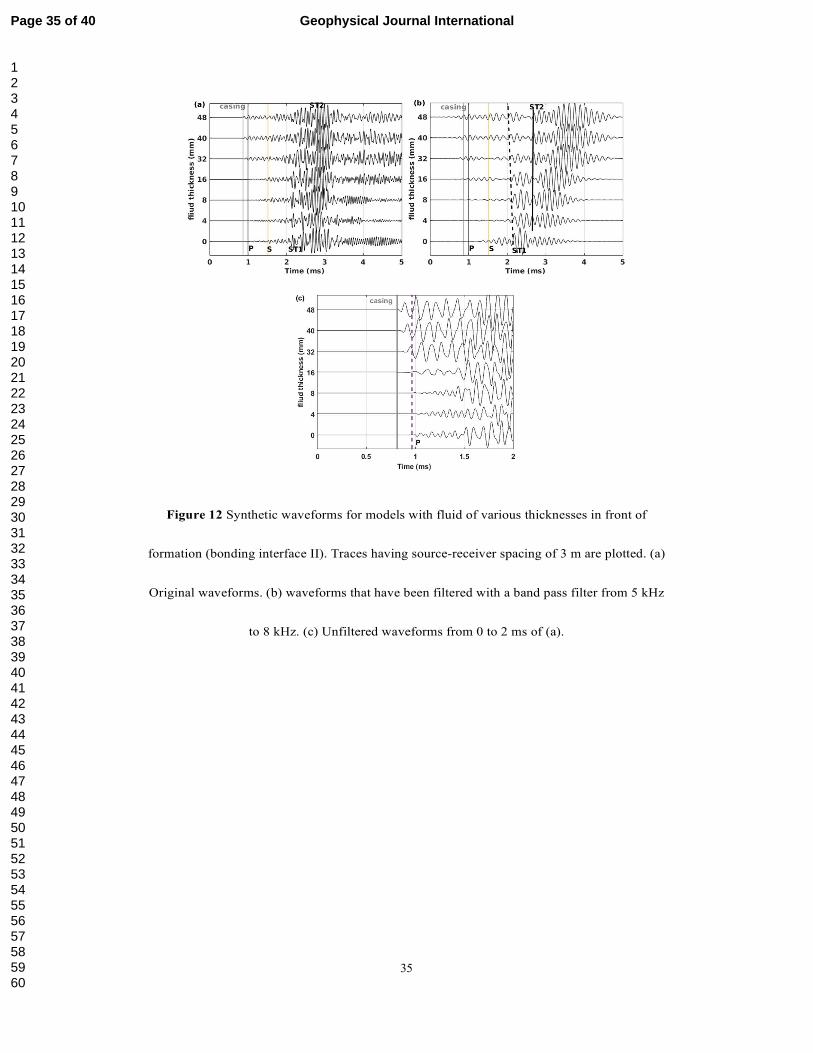
We display the full waveforms in Fig. 12 in the same manner as Fig. 9. In the detailed

display of the waveforms in Fig. 12c we see a clear casing mode (a combination of

casing and cement modes) as the first arrival between the labeled casing and P arrivals

when the cement is partially replaced with fluid. Although the P wave is submerged in

the mode and cannot be discerned when fluid column is large, the mode propagates

with the P velocity when the thickness of fluid column is as small as 4 mm to about

16 mm and its presence could be interpreted as indicating good cement. Fortunately,

we find a clear ST2 in the waveforms, especially those that have been filtered, which

can help us avoid the misinterpretation. Similar to the case of bonding interface I, we

suggest the use of a tool with a large offset to separate the ST2 modes for the thin (4

mm to 8 mm) fluid column cases.


123456789101112131415161718192021222324252627282930313233343536373839404142434445464748495051525354555657585960

16

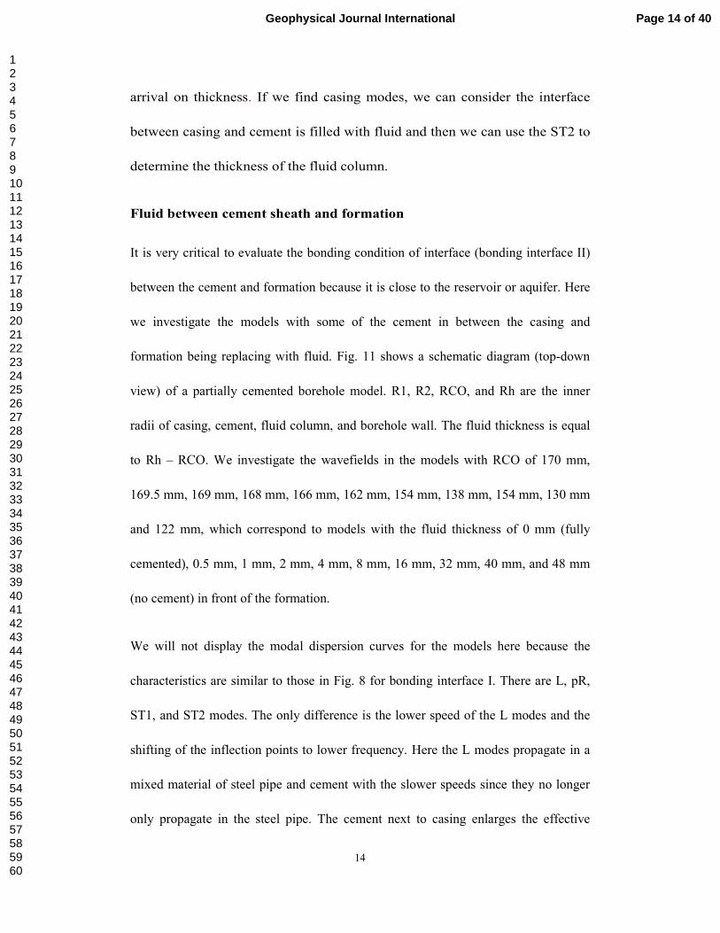
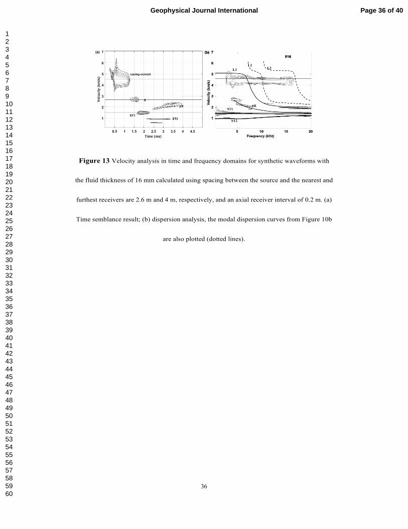
Fig. 13 shows the velocity-time semblance (Fig. 13a) and dispersion analysis (Fig.

13b) plots. From Fig. 13a, we clearly find a casing-cement mode with a velocity

nearly the same as the P velocity in addition to S, ST1, ST2 modes. As mentioned, if

we only use the first arrival (amplitude or velocity) to determine the bonding

condition, we will definitely misjudge the bonding condition as indicating very good

cement even for the fluid column thickness of 16 mm in front of formation. However,

the good coherence for ST2 (from the filtered waveforms) in Fig. 13a gives us an

opportunity to avoid the misjudgment. The dispersion analysis plot in Fig. 13b gives

us another view for mode identification which can also be used to eliminate the

misjudgment. The modal curves (dotted lines) for the model with fluid column

thickness of 16 mm next to the casing is also plotted to illustrate the difference from

Fig. 10b. We find the dispersion characteristics of pR, ST1, and ST2 are the same as

those in Fig. 10b. The casing-cement modes, which will likely be identified as P

waves, have slower velocities than the P wave and the L modes in Fig. 10b.

Our results show that it is necessary to use the full waveform, especially the later part

of the waveforms, to estimate the cement bonding condition when a fluid column

exists next to the formation. A large offset receiver is necessary to make the ST2

visible. Dispersion analysis is also a good tool to eliminate misinterpretation. In field

applications, dispersion analysis may be impractical due to the time it requires. Time

semblance would be also helpful because we could get velocity information about the

ST2 mode which can be a very good indicator for bad bonding condition. Cement

evaluation will be highly improved by using the full waveform.


123456789101112131415161718192021222324252627282930313233343536373839404142434445464748495051525354555657585960

17

Cement inside the fluid columns

To give more detail about the relationship between the waveforms and the thickness

and location of the fluid column and cement sheath, we separate the annulus between

casing and formation into three parts with each part being a different medium (cement

or fluid) with different thickness. By using this model, we simulate the waveforms in

models with cement partially replacing fluid columns at both next to the casing and

the formation. All the waveforms are shown in Fig. 14a and the names for different

models are also listed on the waveforms. The letters ‘f’ and ‘c’ are fluid and cement,

respectively. The number before the letter is the thickness (units in mm) of the

medium. For example, ‘4f16c28f’ means the annulus consists of 4 mm and 28 mm

fluid columns next to the casing and in front of the formation, respectively. In

addition, a 16 mm thick cement layer is placed between the two fluid columns. The

arrival times for different modes are marked by lines. The casing, P, and S waves are

expanded and shown in Fig. 14b. Because a fluid column exists next to the casing, the

arrival time of the casing mode is the same independent on the thickness of the fluid

column. The amplitude of the casing wave changes a little with the changing

thickness of the fluid next to the casing. The current cement bonding evaluation

method is based the relationship between the amplitude of the casing wave and the

fluid column thickness (e.g. Jutten & Corrigall, 1989; Liu et al., 2011; Tang et al.,

2016). However, this method strongly depends on measurements of the amplitude of

the first arrival and could lead to misinterpretation because the amplitude dependence

on fluid column thickness is not strong. Another issue is that we cannot infer the


123456789101112131415161718192021222324252627282930313233343536373839404142434445464748495051525354555657585960

18

bonding condition of the interface between the cement and formation if the cement

next to the casing is partially replaced with fluid.

We also find little difference in the ST waves (inside the rectangle in Fig. 14a) with

various fluid thicknesses. The dispersion analysis (contour) plots for the waveforms

from different models are shown in from Figs. 14c to 14g. We do not calculate the

modal dispersion curves for the models we simulated here. However, we plot the

modal dispersion curves for the model in Fig. 7. The green lines are the dispersion

curves for a model (Fig. 7) with a 32 mm fluid column between casing and cement.

The black lines are the dispersion curves for a model (Fig. 7) with the fluid thickness

of 4 mm (Fig. 14c), 8 mm (Fig. 14d), 16 mm (Fig. 14e), 24 mm (Fig. 14f) and 28 mm

(Fig. 14g). It is obvious that the green lines for mode ST2 match the dispersion

contour plots for all fluid column thicknesses. This suggests that the ST2 wave can be

used to determine the total thickness of the fluid column in the annulus and it is not

just sensitive to the fluid thickness next to the casing if there is another fluid column

between cement and formation. This may be considered to be a limitation of the

application of the ST2 wave. However, it would be a great supplement for the current

first arrival amplitude method. We can use the amplitude of the casing wave to

determine the fluid thickness next to the casing although sometime this method will

not work very well. We can get the total fluid thickness in the annulus by comparing

the velocity or dispersion curves with the modal cases. Then we can know the

distribution of the fluid in the annulus. This overcomes the limitation of the current

amplitude method on the bonding condition of the interface between cement and


123456789101112131415161718192021222324252627282930313233343536373839404142434445464748495051525354555657585960

19

formation and can also eliminate an ambiguous interpretation.

Fluid inside cement sheath

We also consider the model with fluid column inside of the cement sheath and the

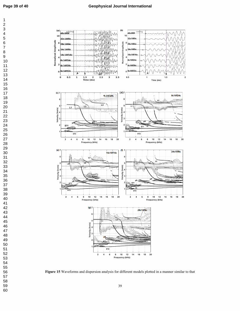
varying thickness of cement next to the casing and in front of the formation. Fig. 15

shows the waveforms and dispersion analysis for different models. The placement of

the subfigures is the same as Fig. 14. Model names are as described for Fig. 14. Fig.

15a shows the full waveforms (3 m offset) for different models and the first 2 ms

waveforms are zoomed in and shown in Fig. 15b. We find that the thickness of

cement next to the casing will definitely affect the arrival time (marked by circles in

Fig. 15b) and amplitude of the first arrival (the mode propagating in the combined

casing and cement of different thickness). As we analyzed in previous section, the

arrival time (velocity) method (Zhang et al., 2013) will not work well when the

cement sheath thickness is large (e.g. 24c16f8c in Fig. 15b). However, the variation in

the first arrival amplitude can be easily discerned and this can be used as an indicator

for thickness of the cement sheath next to the casing. For the ST waves (marked with

a rectangle in Fig. 15a), we find it is not sensitive to the cement sheath thickness,

which means the ST2 wave is not sensitive to the location of the fluid column. The

dispersion contour plots are shown in Figs. 15c to 15g (modal dispersion curves for

16 mm fluid column existing in interface I is plotted with back lines). We find a good

match between the dispersion contours of ST2 with those for the model shown in Fig.

11 (the fluid column thickness of 16 mm). This good match leads us to infer that the

ST2 wave is only sensitive to the fluid thickness not the fluid location.


123456789101112131415161718192021222324252627282930313233343536373839404142434445464748495051525354555657585960

20

CONCLUSIONS

We have used a 3DFD method to simulate wave propagation from a

monopole source in a singly-cased borehole with different bonding conditions.

Pressure snapshots of the wavefields give us a direct way to evaluate wave

excitation and propagation for different models. Data processing methods

such as velocity-time semblance and dispersion analysis facilitate the

identification of the modes in the different models. Our conclusions are as

follows,

(1) The formation modes can be easily discerned when the casing is well

bonded. However, the P wave is submerged in the casing mode and the S

wave has poor coherence when the cement is replaced with fluid.

(2) The amplitude of casing modes can be used for determine the bonding

condition of the interface between casing and cement. However, the small

variation of first arrival amplitude with thickness of fluid between casing and

cement could introduce ambiguity in the interpretation.

(3) When using only the arrival time (velocity) of the first arrival, it would be

highly likely that the presence of fluid between the casing and the cement

would be misjudged as good cement. The amplitude of the first arrival is a

much better indicator.


123456789101112131415161718192021222324252627282930313233343536373839404142434445464748495051525354555657585960

21

(4) The slow Stoneley (ST2) mode can be used to evaluate the total thickness

of the fluid column in the annulus no matter where the fluid column is located

even there are two fluid columns.

(5) Analysis of the full waveform by combining the first arrival and the slow

ST waves can be used eliminate the ambiguity about cement condition and

improve cement evaluation reliability compared to the current method using only

first arrival measurements.

ACKNOWLEDGEMENTS

This study is supported by the Founding Members Consortium of the Earth resources

Laboratory at MIT.

REFERENCES

Byun, J., M. N. Toksöz, 2003, Analysis of the acoustic wavefields excited by the

Logging-While-Drilling (LWD) tool: Geosytem Eng., 6(1), 19-25.

Cawley P, Lowe M, Simonetti F, Chevalier C, Roosenbran A, 2002, The variation of

reflection coefficient of extensional guided waves in pipes from defects as a function of

defect depth, axial extent, circumferential extent and frequency. J.Mech.Eng.Sci,

216:1131-1143.

Daley T., Freifeld B., Ajo-Franklin J., Dou S., Pevzner R., Shulakove V., Kashikar S., Miller

D., Goetz J., Lueth S., 2013, Field testing of fiber-optic distributed acoustic sensing (DAS)

for subsurface seismic monitoring, The Leading Edge, 6,936-942

Jutten J., and Corrigall E., 1989, Studies with narrow cement thickness lead to improved CBL

in concentric casings: J. Pet. Tech. 11, 1158-1192.

Kimball, C.V., T. Marzetta, 1986, Semblance processing of borehole acoustic array data:

Geophysics, 49:274-281.

Lecampion B., Quesada D., Loizzo M., Bunger A., Kear J., Deremble L., Desroches J. (2011),

Interface debonding as a controlling mechanism for loss of well integrity: Importance for

CO2 injector wells, Energy Procedia, 4, 5219-5226.


123456789101112131415161718192021222324252627282930313233343536373839404142434445464748495051525354555657585960

22

Liu X., Chen D., Chen H., Wang X., 2011, The effects of the fluid annulus thickness at the

first interface on the casing wave: Technical Acoustics, 30(4),301-305.

Marzetta, T. and M. Schoenberg, 1985, Tube waves in cased boreholes: 55th Annual

International Meeting, SEG, Expanded Abstracts, 34–36. DOI:10.1190/1.1892647.

Pardue G. H., Morris R. L., Gollwitzer L. H., Moran J. H., 1963, “Cement Bond Log - A

study of cement and casing variables”, J. Pet. Tech. 5, 545-555.

Paillet, F., and C. H., Cheng, 1991, Acoustic waves in boreholes, P.154, CRC Press.

Plona, T., B. K., Sinha, S., Kostek, and S. K., Chang, 1992, Axisymmetric wave propagation

in fluid-loaded cylindrical shells. II: Theory versus experiment, J. Acoust. Soc. Am., 92(2):

1144-1155.

Tang J., Zhang C., Zhang B., Shi F., 2016, Cement bond quality evaluation based on acoustic

variable density logging: Petroleum exploration and development, 43(3), 514-521.

Tubman, K. M., Cole, S. P., Cheng, C. H., Toksöz, M. N., 1984, Dispersion curves and

synthetic microseismograms in unbonded cased boreholes, Earth Resources Laboratory

Industry Consortia Annual Report, 1984-02.

Walker, T., 1968, A full-wave diplay of acoustic signal in cased holes, SPE 1751.

Wang, H., G., Tao, and M. C., Fehler, 2015, Investigation of the high-frequency wavefield of

an off-center monopole acoustic logging-while-drilling tool, GEOPHYSICS, 80(4):

D329-D341.

Wang, H., G., Tao, X., Shang, 2016, Understanding acoustic methods for cement bond

logging, J. Acoust. Soc. Am. 139(5), 2407-2416. DOI: 10.1121/1.4947511

Zhang, H., D., Xie, Z., Shang, X., Yang, H., Wang, H., Tao, 2011, Simulated various

characteristic waves in acoustic full waveform relating to cement bond on the secondary

interface, Journal of Applied Geophysics, 73(2), 139-154.

Zhang, X., Wang, X., Zhang, H., 2016, Leaky modes and the first arrivals in cased boreholes

with poorly bonded conditions, Science China-Physics, Mechanics & Astronomy, 59(2),

624301.


123456789101112131415161718192021222324252627282930313233343536373839404142434445464748495051525354555657585960

23

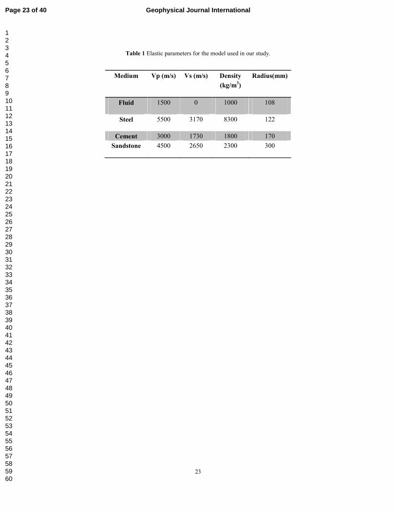
Table 1 Elastic parameters for the model used in our study.

Medium Vp (m/s) Vs (m/s) Density

(kg/m3)

Radius(mm)

Fluid 1500 0 1000 108

Steel 5500 3170 8300 122

Cement 3000 1730 1800 170

Sandstone 4500 2650 2300 300


123456789101112131415161718192021222324252627282930313233343536373839404142434445464748495051525354555657585960

24

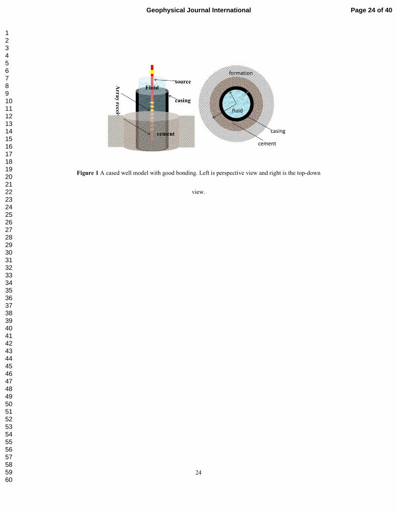
Figure 1 A cased well model with good bonding. Left is perspective view and right is the top-down

view.


123456789101112131415161718192021222324252627282930313233343536373839404142434445464748495051525354555657585960

25

Figure 2 Comparison between the 3DFD and DWM simulations in a free casing model: (a) Array

waveforms; (b) velocity-time semblance plot for the array waveforms in (a).


123456789101112131415161718192021222324252627282930313233343536373839404142434445464748495051525354555657585960

26

Figure 3 (a) X-Z profile of the model: (a) Single casing model with a perfect cement bond. Colors

blue, red, light blue and orange are fluid, steel casing, cement and formation, respectively. Pressure

snapshots for situations where the (b) cement is perfect bonded, (c) free casing and (d) casing

immersed in fluid.


123456789101112131415161718192021222324252627282930313233343536373839404142434445464748495051525354555657585960

27

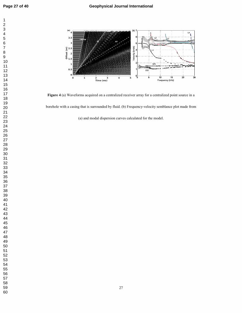
Figure 4 (a) Waveforms acquired on a centralized receiver array for a centralized point source in a

borehole with a casing that is surrounded by fluid. (b) Frequency-velocity semblance plot made from

(a) and modal dispersion curves calculated for the model.


123456789101112131415161718192021222324252627282930313233343536373839404142434445464748495051525354555657585960

28

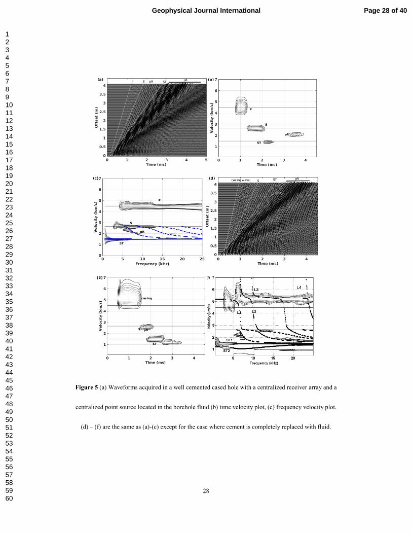
Figure 5 (a) Waveforms acquired in a well cemented cased hole with a centralized receiver array and a

centralized point source located in the borehole fluid (b) time velocity plot, (c) frequency velocity plot.

(d) – (f) are the same as (a)-(c) except for the case where cement is completely replaced with fluid.


123456789101112131415161718192021222324252627282930313233343536373839404142434445464748495051525354555657585960

29

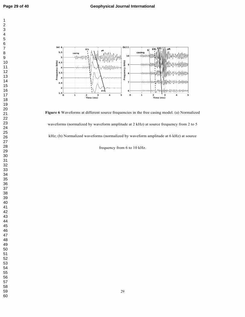
Figure 6 Waveforms at different source frequencies in the free casing model. (a) Normalized

waveforms (normalized by waveform amplitude at 2 kHz) at source frequency from 2 to 5

kHz; (b) Normalized waveforms (normalized by waveform amplitude at 6 kHz) at source

frequency from 6 to 10 kHz.


123456789101112131415161718192021222324252627282930313233343536373839404142434445464748495051525354555657585960

30

Figure 7 Schematic diagrams (top-down view) of a partially cemented borehole model (bad bonding

for interface I). R1, R2, RCI, Rh are the inner radii of casing, fluid column, cement, and borehole wall.

The fluid thickness is equal to RCI – R2. R1, R2, and Rh are given in Table 1.


123456789101112131415161718192021222324252627282930313233343536373839404142434445464748495051525354555657585960

31

Figure 8 Dispersion curves of ST2, L and pR modes with various fluid thicknesses between

casing and cement (bonding interface I). (a) ST2 modes, fluid thicknesses are marked; (b) L

and pR modes, the legends for different lines are given and the black dot-lines are the free

bonding case (the fluid thickness of 48 mm).


123456789101112131415161718192021222324252627282930313233343536373839404142434445464748495051525354555657585960

32

Figure 9 Synthetic waveforms for the models with fluid of various thicknesses between the

casing and cement (bonding interface I). Traces with source-receiver spacing of 3 m are

plotted. (a) Original waveforms; (b) waveforms filtered with a band pass filter from 5 kHz to

8 kHz.


123456789101112131415161718192021222324252627282930313233343536373839404142434445464748495051525354555657585960

33

Figure 10 Velocity analysis in time and frequency domains for the synthetic waveforms with

the fluid thickness of 16 mm (the spacing between the source and the nearest and furthest

receivers are 2.6 m and 4 m, respectively, and the axial receiver interval is 0.2 m). (a) Time

semblance result; (b) dispersion analysis, the modal dispersion curves are also plotted (dot

lines).


123456789101112131415161718192021222324252627282930313233343536373839404142434445464748495051525354555657585960

34

Figure 11 Schematic diagram (top-down view) of a partially cemented borehole model. R1, R2, RCO,

and Rh are the inner radii of casing, cement, fluid column, and borehole wall. The fluid thickness is

equal to Rh – RCO.


123456789101112131415161718192021222324252627282930313233343536373839404142434445464748495051525354555657585960

35

Figure 12 Synthetic waveforms for models with fluid of various thicknesses in front of

formation (bonding interface II). Traces having source-receiver spacing of 3 m are plotted. (a)

Original waveforms. (b) waveforms that have been filtered with a band pass filter from 5 kHz

to 8 kHz. (c) Unfiltered waveforms from 0 to 2 ms of (a).


123456789101112131415161718192021222324252627282930313233343536373839404142434445464748495051525354555657585960

36

Figure 13 Velocity analysis in time and frequency domains for synthetic waveforms with

the fluid thickness of 16 mm calculated using spacing between the source and the nearest and

furthest receivers are 2.6 m and 4 m, respectively, and an axial receiver interval of 0.2 m. (a)

Time semblance result; (b) dispersion analysis, the modal dispersion curves from Figure 10b

are also plotted (dotted lines).


123456789101112131415161718192021222324252627282930313233343536373839404142434445464748495051525354555657585960

37

Figure 14 Waveforms and dispersion analysis for different models. (a) waveforms (3m offset) for


123456789101112131415161718192021222324252627282930313233343536373839404142434445464748495051525354555657585960

38

different models. Names for different models are listed on the waveforms. The letters ‘f’ and ‘c’ are

fluid and ‘c’, respectively. The number before the letter is the thickness (unit in mm) of the medium.

For example, ‘4f16c28f’ means the annulus consists of 4 mm and 28 mm fluid columns next to casing

and in front of formation, respectively. And cement with 16 mm is filled between the two fluid

columns. (b)Normalized waveforms of the first 2 ms. (c)-(g) dispersion analysis plots for the

waveforms in different models. The green lines are the dispersion curves for model (Figure 7) with a

32 mm fluid column between casing and cement. The black lines are the dispersion curves for model

(Figure 7) with the fluid thickness of 4 mm (Figure 14c), 8 mm (Figure 14d), 16 mm (Figure 14e), 24

mm (Figure 14f) and 28 mm (Figure 14g).


123456789101112131415161718192021222324252627282930313233343536373839404142434445464748495051525354555657585960

39

Figure 15 Waveforms and dispersion analysis for different models plotted in a manner similar to that


123456789101112131415161718192021222324252627282930313233343536373839404142434445464748495051525354555657585960

40

in Figure 14. (a) waveforms (3m offset) for different models. (b)Normalized waveforms of the first 2

ms. Arrival times of the first arrival are marked with circles. (c)-(g) dispersion analysis plots for the

waveforms for different models.


123456789101112131415161718192021222324252627282930313233343536373839404142434445464748495051525354555657585960

Documents

THE WAV EFIELD OF ACOUSTIC LOGGING IN A … Wavefield...5 6 7 8 9 10 11 12 13 14 15 16 17 18 19 20 21 22 23 24 25 26 27 28 29 30 31 32 33 34 35 36 37 38 39 40 41 42 43 44 45 46 47