The Welfare Effects of Balance of Payments Reform: A Macro ...shanda/research/micro_macro_jds_2003.pdf · selected balance of payment reforms, ... consequences of trade and payments

The Welfare Effects of Balance of PaymentsReform: A Macro–Micro Simulation

of the Cost of Rent-Seeking

DAMIEN KING and SUDHANSHU HANDA

This article proposes a methodology for analysing the effect ofbalance of payments liberalisation on measures of poverty anddistribution and applies it to the case of Jamaica in the 1990s. Themethodology consists of a macro–micro simulation in which aCGE model provides labour market outcomes, which in turn areused to manipulate the sectoral allocation of employment togenerate the income distribution consistent with the new labourmarket outcome. In the application to Jamaica, we find that thereallocation of resources away from rent-seeking activities in thepresence of exchange controls is significant and has largemacroeconomic effects. Opening up of the current account haslittle effect on poverty, but liberalisation of the capital accountreduces poverty, especially amongst the very poor. Neither policychange taken separately, nor the combination of the two, has morethan a negligible effect on the distribution of income.

I . INTRODUCTION

Over the more than two decades that Latin America and the Caribbean havebeen implementing structural adjustment programmes, there has been muchconcern over the human impact of policy reform [Addison, 1994; Prasad,1998]. In this regard, balance of payments reform has generated the greatestconcern. But balance of payments reform has usually been implemented in

Damien King, Department of Economics, University of the West Indies, Kingston 7, Jamaica;email: [email protected]; Sudhanshu Handa, Inter-American Development Bank,Washington, DC 20006, USA; email: [email protected]. This research was originally carriedout as a part of the UNDP/ ECLACL/IDB project on ‘Balance of Payments Liberalization:Effects on Employment Distribution, Poverty and Growth’. The authors are grateful to ShermanRobinson for comments on an earlier version, Ricardo Paes de Barros for guidance on parts ofthe methodology employed in the article, Enrique Ganuza for the origin of the idea for thisresearch, and the participants at the project’s conference in Buenos Aires, Argentina, 3–5February 2000 along with this journal’s anonymous referees for helpful comments.

The Journal of Development Studies, Vol.39, No.3, February 2003, pp.101–128PUBLISHED BY FRANK CASS, LONDON

393jds05.qxd 17/02/2003 09:33 Page 101

concert with financial liberalisation, public sector reform, labour marketreform, stabilisation, and other elements of the structural adjustment policypackage. The difficulty in assessing the effect of any particular element ofreform is in separating its impact from the other policy changes andexogenous shocks occurring at the same time. The present article uses aquantitative simulation as a means of separating and measuring the impactof balance of payments reform on welfare and distribution. Themethodology consists of a macro-component based on a computablegeneral equilibrium model which simulates the labor market outcomes ofselected balance of payment reforms, and a household level componentwhich simulates the welfare consequences of these new labour marketoutcomes. The results are driven by our modeling of the rent-seekingconsequences of trade and payments restrictions.

The methodology is applied to the case of Jamaica in the 1990s, anappropriate test case given the peculiarities of growth and povertyoutcomes there. Jamaica was one of the worst economic performers in theLatin American and Caribbean region during the 1990s. After almost twodecades of economic reform, sporadically and unevenly implemented[King, 2001], including sweeping balance of payments reform between1991 and 1998, the average annual growth rate of real GDP over that timewas zero. At the same time, measures of poverty and distribution have notshown the dramatic worsening that one would have expected in the contextof such poor macroeconomic performance. On the contrary,notwithstanding some volatility in the measures of poverty, householdsurvey data suggest a clear reduction in poverty over the period. Forinequality, there was a sudden decline in the Gini coefficient between 1989and 1991, and then only a very gradual decline up to 1997, after which itappears to have stabilised.

This has been a period of significant economic reform in Jamaica,dominated by the liberalisation of the balance of payments, but alsoincluding stabilisation policy which was pursued in earnest over the sameperiod. The methodology employed below generates a counter-factualscenario to isolate the role of reform policy, in this case the reform of tradeand payments, on the poverty and income distribution outcomes that havebeen observed. This is accomplished by combining simulations from a CGEmodel with hypothetical redistributions of households amongst sectors. Themodel’s simulations are used to produce a profile of the labour market. Theprofile includes the distribution of employment amongst the productivesectors, the amount of unemployment, and the wage structure by labourmarket segment. The simulated labor market profile (LMP) is imposed uponhousehold survey data to generate a hypothetical distribution of householdsfrom which inferences about the poverty and distributional consequences of

102 THE JOURNAL OF DEVELOPMENT STUDIES

393jds05.qxd 17/02/2003 09:33 Page 102

policy actions is drawn. Our main results indicate that the sweeping balanceof payments liberalisation that occurred in Jamaica during the 1990s mayindeed have had a positive effect on poverty. For example, the policysimulations show that capital account liberalization decreased the extremepoverty headcount ratio by two percentage points, with the strongest effectscoming from changes in relative wages. These results may partially accountfor the empirically observed ‘paradox’ of low growth and declining povertyin Jamaica during this period.

The article makes several contributions to the literature on the welfareeffects of structural adjustment policies. First, unlike previouswork, international payments restrictions are modelled as inducing rent-seeking behaviour within the economy, while the common practice isto treat these restrictions as an exogenous change in foreign capital inflows.Second, instead of merely simulating aggregate macroeconomic outcomesusing the CGE as in most of the previous work, we go a step further byspecifying a mechanism to explicitly link the CGE outcomes to micro-survey data so as to simulate the impact of policy reforms on the distributionof welfare. In this way we exploit the strength of the CGE (its ability toisolate the impact of specific policy reforms) and the strength of micro-survey data (more reliable estimates of poverty and inequality) in order toinvestigate the link between specific structural adjustment policies andindividual welfare.

The article is organised as follows. Section I describes the Jamaicaneconomic context – the evolution of poverty and income distribution, thecharacter of the labour market, and the policy context in which the balanceof payments was liberalised. Section II describes the macro-model as wellas the policy scenarios explored, and presents the results of CGEsimulations. The third section explains the micro simulation methodologyand presents the computation of household welfare and sectoral allocationsthat would obtain in the event the policy scenarios were implemented.

II . THE CONTEXT FOR THE SIMULATIONS

Poverty and Distribution

We describe the evolution of welfare in Jamaica using the Survey of LivingConditions (SLC), a nationally representative household survey collectedannually since 1989 by the Statistical Institute of Jamaica (STATIN). Themeasure of household welfare used in the SLC and by the Planning Instituteof Jamaica in computing national poverty rates is per capita householdconsumption expenditure. Total household consumption is constructed bySTATIN based on the monetary value of consumption expenditure provided

103WELFARE EFFECTS OF BALANCE OF PAYMENTS REFORM

393jds05.qxd 17/02/2003 09:33 Page 103

in the relevant modules of the SLC, and is divided by the number ofhousehold members as reported in the household roster. Because ourobjective is to track the evolution of welfare over time, we avoid the potentialcontroversy of defining an absolute poverty line, and instead use a relativepoverty line set at the 25th percentile of the distribution of per capitaconsumption in 1989. This line is the Jamaican dollar equivalent of annualper capita consumption of US$409, inflated by the CPI for subsequent years.The information presented below is drawn from six years of SLC data,beginning in 1989, and including 1991, 1992, 1993, 1995 and 1998.

Table 1 provides estimates of mean and median consumption, headcountratios, and Gini coefficients for the selected years. Poverty increased in


TABLE 1WELFARE INDICATORS

1989 1991 1992 1993 1995 1998

Mean Consumption 6,407 5,344 4,799 5,808 5,493 6,290(constant J$)Median Consumption 4,594 4,034 3,580 4,496 4,137 4,778(constant J$)Headcount 25.00 27.31 31.92 20.73 22.27 16.65Gini Coefficient 0.436 0.403 0.396 0.382 0.375 0.381

Note: All indicators are based on per capita household consumption expenditures, deflated to1989 Jamaican dollars. Data are from the Survey of Living Conditions.

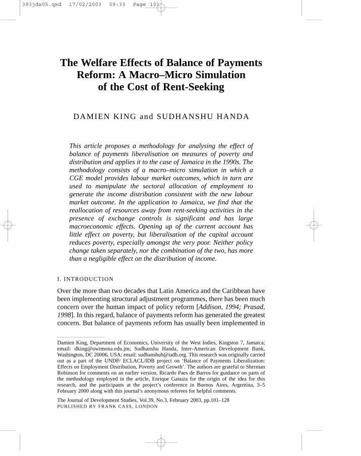
TABLE 2POVERTY RATES BY YEAR AND GROUP

Year: 1989 1991 1992 1993 1995 1998

RegionKMA 5.73 9.67 14.72 11.73 10.9 6.64TOWN 13.39 19.12 22.72 17.12 17.56 12RURAL 35.68 39.23 40.96 27.6 31.31 21.96Head’s SchoolingNone 48.61 27.82 43.22 26.61 33.84 21.95Some Primary 30.72 28.5 44.05 34.43 33.23 24.38CompletePrimary 27.55 37.44 38.56 24.39 26.94 19.3Grade 9 26.60 20.28 26.26 20.41 23.25 14.75Grade 11 9.24 10.53 14.37 12.96 9.91 8.98A level or higher 5.32 12.09 14.2 2.01 2.27 8.06Head’s IndustryAgriculture-Tradable 40.52 42.25 36.96 20.67 46.36 24.18Agriculture-Non Tradable 39.40 47.44 44.13 36.66 38.5 25.04Mining 0.00 0 18.98 10.45 0 22.54Manufacturing 20.43 13.95 25.87 12.29 13.76 10.36Services-Tradable 15.99 10.19 13.78 8.88 11.79 4.99Services Non Tradable 17.51 20.64 26.03 13.66 17.07 13.14

Note: Authors’ calculations based on the Survey of Living Conditions.

393jds05.qxd 17/02/2003 09:33 Page 104

1991 and 1992, when there was a dramatic rise in the inflation rate uponimplementation of financial sector reforms and exchange rate liberalisation.Since the reforms, poverty has been on the decline, reaching its lowest levelin the most recent survey year (16.7 per cent in 1998). Between 1993 and1996, this improvement in poverty probably derived from nominal wagescatching up with prices following the inflation surge of 1991/92 (the reasonfor the rise in real wages is discussed below). Mean and medianconsumption tend to follow the poverty rate, rising when poverty falls (1993and 1998) and falling when poverty rises (1991, 1992, and 1995).

Table 2 provides poverty rates by sub-groups over this time period. Thesalient features of poverty in Jamaica are that rural residents are muchpoorer than the average, and that poverty rates decline significantly amonghouseholds where the head has at least a grade 11 education (thiscorresponds to second cycle secondary schooling in Jamaica).1 Finally,households whose principal earner works in a non-tradable sector are alsolikely to be poorer than the average. In fact, 86 per cent of the poor live inhouseholds whose head works in either the services or agricultural non-tradable sectors (results not shown but available upon request). It is alsonoteworthy that urban households, and households whose heads had morethan grade 11 schooling, registered significant increases in poverty rates inthe years of high inflation (1991–92).

The Gini coefficient declined significantly over the period, falling froma high of 0.436 in 1989 to 0.381 in 1998. Consistent with a decline ininequality, the difference between the lowest and highest poverty incidencebetween some groups is smaller in 1998 than in 1989. For education ofhead, for example, only 16 percentage points (24.4–8.1) separates thehighest and the lowest, compared to 43 percentage points in 1989 (48.6–5.3), indicating that the importance of schooling seems to have declined interms of determining poverty.

The Labour Market

In the methodology presented below, the labour market profile is the linkbetween the macroeconomy and the distribution of labour income. It isimportant, therefore, to characterise the labour market in Jamaica in orderto ensure that the simplifications embodied in the specifications belowreflect the most instructive view of the labour market. In particular, the mostuseful segmentations need to be established.

At a casual level of observation, all the expected ‘dualities’ are presentin the labour market in Jamaica. There is a large informal sector. The labourforce surveys during the 1990s classify between 35 and 40 per cent asworking on their ‘own-account’, which is to say, not receiving an explicit


393jds05.qxd 17/02/2003 09:33 Page 105

salary but instead living on the proceeds of their activity. Panton (1993)reports 47 per cent of the employed labor force engaged in informal activity.

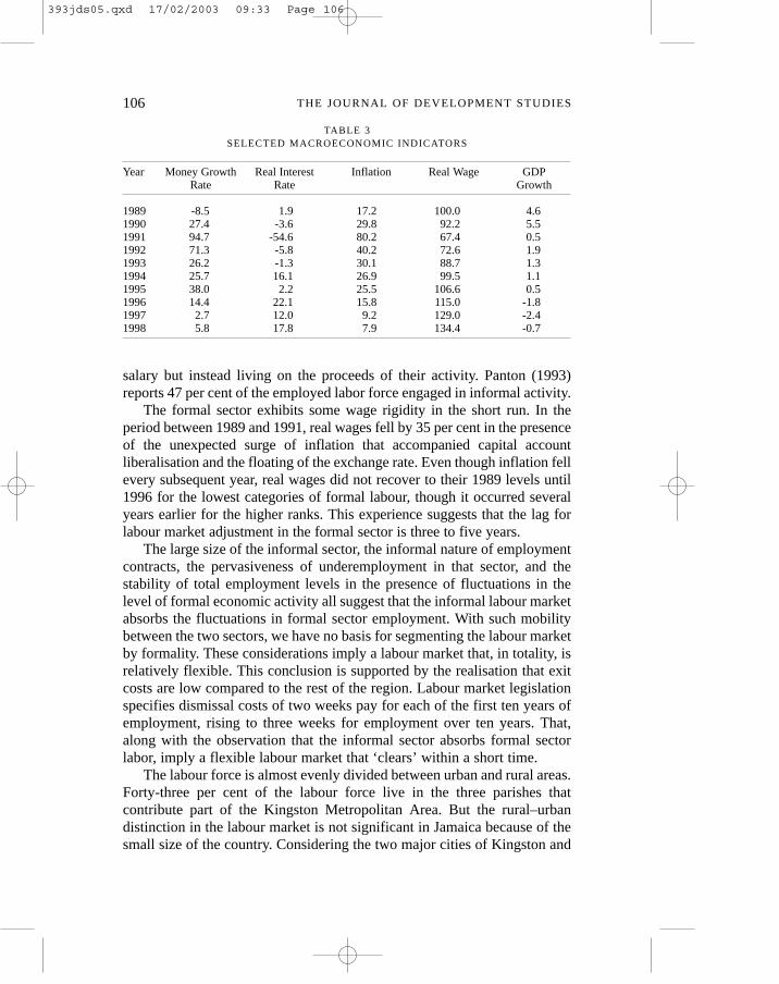
The formal sector exhibits some wage rigidity in the short run. In theperiod between 1989 and 1991, real wages fell by 35 per cent in the presenceof the unexpected surge of inflation that accompanied capital accountliberalisation and the floating of the exchange rate. Even though inflation fellevery subsequent year, real wages did not recover to their 1989 levels until1996 for the lowest categories of formal labour, though it occurred severalyears earlier for the higher ranks. This experience suggests that the lag forlabour market adjustment in the formal sector is three to five years.

The large size of the informal sector, the informal nature of employmentcontracts, the pervasiveness of underemployment in that sector, and thestability of total employment levels in the presence of fluctuations in thelevel of formal economic activity all suggest that the informal labour marketabsorbs the fluctuations in formal sector employment. With such mobilitybetween the two sectors, we have no basis for segmenting the labour marketby formality. These considerations imply a labour market that, in totality, isrelatively flexible. This conclusion is supported by the realisation that exitcosts are low compared to the rest of the region. Labour market legislationspecifies dismissal costs of two weeks pay for each of the first ten years ofemployment, rising to three weeks for employment over ten years. That,along with the observation that the informal sector absorbs formal sectorlabor, imply a flexible labour market that ‘clears’ within a short time.

The labour force is almost evenly divided between urban and rural areas.Forty-three per cent of the labour force live in the three parishes thatcontribute part of the Kingston Metropolitan Area. But the rural–urbandistinction in the labour market is not significant in Jamaica because of thesmall size of the country. Considering the two major cities of Kingston and


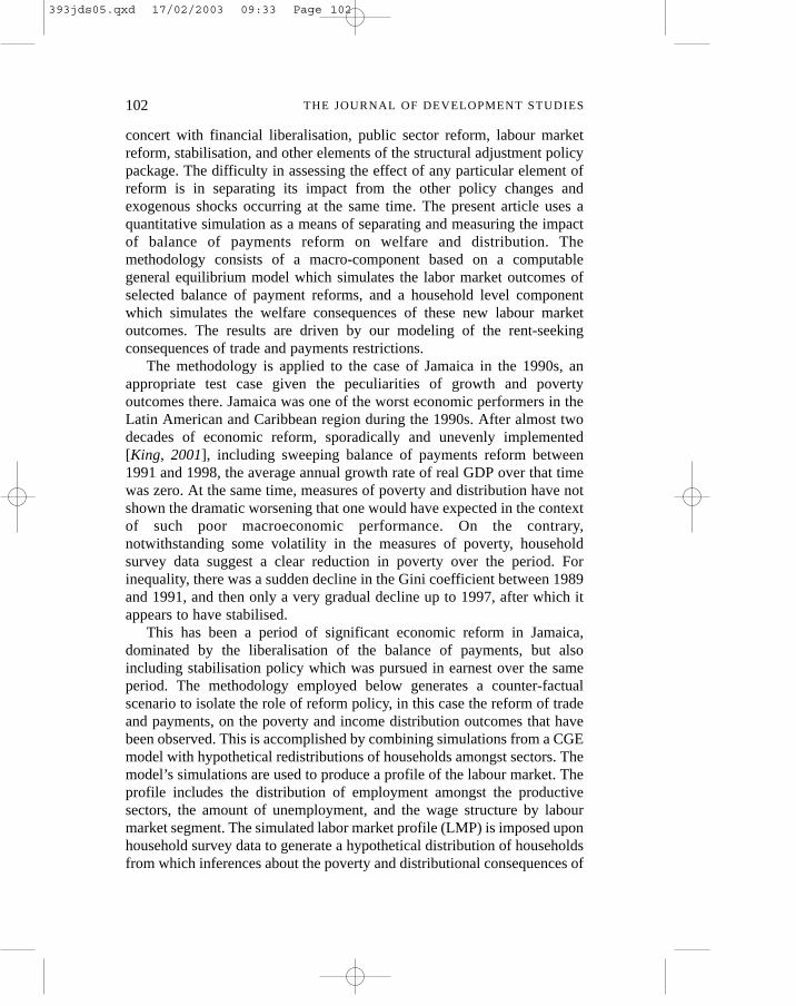
TABLE 3SELECTED MACROECONOMIC INDICATORS

Year Money Growth Real Interest Inflation Real Wage GDPRate Rate Growth

1989 -8.5 1.9 17.2 100.0 4.61990 27.4 -3.6 29.8 92.2 5.51991 94.7 -54.6 80.2 67.4 0.51992 71.3 -5.8 40.2 72.6 1.91993 26.2 -1.3 30.1 88.7 1.31994 25.7 16.1 26.9 99.5 1.11995 38.0 2.2 25.5 106.6 0.51996 14.4 22.1 15.8 115.0 -1.81997 2.7 12.0 9.2 129.0 -2.41998 5.8 17.8 7.9 134.4 -0.7

393jds05.qxd 17/02/2003 09:33 Page 106

Montego Bay, no rural area is more than two hours by car from one of thethem. This suggests that the wage differential between rural and urban forcorresponding occupations would not become very great before inducingmigration. Further, the personal dislocation of the migration is would not besignificant since one can return ‘home’ for weekends.

The labour force in 1990 prior to economic reform was (and is) largelyunskilled and engaged in informal activities. The labour force surveysreveal that near 80 per cent of the labor force has no education or trainingbeyond high school, not even ‘on-the-job’ training. There is a substantialskill premium, an unsurprising result in light of the scarcity of skills. Giventhe socio-economic basis of much of the skill differentiation, the length oftime and cost of skill enhancement, and the observed high level of the skillpremium, there can be no mobility across the skill divide, so we segment thelabour market by skill. And given the large number of unskilled, only twoskill levels are sufficient.

The unemployment rate for much of the 1990s has been between 14 to17 per cent. In order to model the labour market in the CGE, it is necessaryto understand the nature of this portion of the labour force classified asunemployed. We reject the idea that the unemployed in Jamaica are a readypool of surplus productive capacity idled by rigid wages that are above themarket-clearing level, in favour of the interpretation that the observedunemployed largely represent the natural rate of unemployment. Thisconclusion is based on two considerations. First, a disaggregation of labourforce by duration of unemployment, from the October 1990 survey, revealsthat 76.3 per cent of the unemployed have not worked in over a year, andmore than half that number have never held a job. By the October 1998survey, that figure was still as high as 63.4 per cent. Therefore, theunemployed, as in most of Latin America and the Caribbean, are largely an


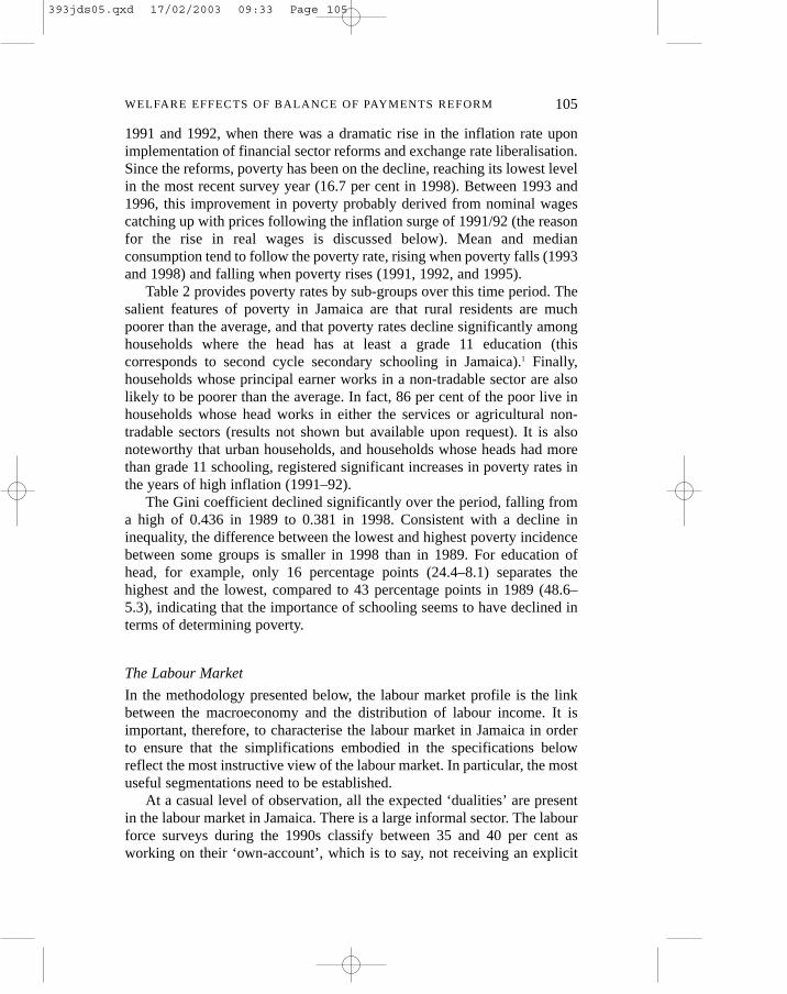
TABLE 4SECTORAL STRUCTURE OF GDP AND EMPLOYMENT

GDP EmploymentAgri- Mining Manu- Finance Services Agri- Mining Manu- Finance Services

culture facturing culture facturing

1993 7.8 6.2 17.5 6.6 61.9 24.6 0.9 10.9 4.8 58.81994 8.4 6.7 17.2 8.6 59.0 24.0 0.7 10.4 5.1 59.71995 8.6 6.6 16.2 8.4 60.2 24.3 0.8 11.4 5.6 57.91996 7.7 5.5 15.6 8.5 62.8 22.7 0.7 10.5 5.7 60.51997 7.5 5.2 15.0 7.1 65.2 21.8 0.6 9.4 6.3 61.91998 7.5 4.6 14.1 7.1 66.8 21.4 0.6 8.8 6.0 63.2

Sources: National Income and Product Accounts, Statistical Institute of Jamaica, various years;The Labour Force, Statistical Institute of Jamaica, various issues.

393jds05.qxd 17/02/2003 09:33 Page 107

unchanging group of long-term unemployed. Second, the unemploymentrate has not been below 14 per cent since at least the early 1960s – a periodof almost 40 years.

The Jamaica labour market therefore, may be characterised in thefollowing way. The labor force is engaged in both formal and informalactivities but cannot be segmented by formality. The informal sector ensuresflexibility in the labour market, notwithstanding backward looking wagecontracts in the formal sector. About half the labour force works in ruralareas, but again there is fluidity of labour movement. The labour force islargely unskilled which gives rise to a high skill premium.

The Policy Context

Jamaica has been a part of stabilisation and structural adjustmentprogrammes since it signed its first Stand By Agreement with the IMF in1977. Since then, its implementation of structural economic reform hasbeen lukewarm, at best [Handa and King, 1997; King, 2001].

Prior to 1990, reform consisted largely of fiscal retrenchment and sometariff reduction. Government expenditure, which was as high as 35 per centof GDP in 1980, steadily fell until 1989 when it stood at 22 per cent. The


TABLE 5INDICATORS OF TRADE LIBERALISATION

Average Import Tariff (%) Standard Deviation of Tariffs

1980 25.7 24.31981 25.0 20.71982 25.0 20.71983 25.0 20.71984 25.0 20.71985 25.0 20.71986 25.0 20.71987 25.0 20.71988 25.0 20.71989 25.0 20.71990 25.0 20.71991 22.1 16.81992 22.1 16.81993 15.9 13.41994 15.9 13.41995 14.0 13.41996 14.0 13.41997 14.0 13.41998 11.8 14.7

Source: Authors’ calculation, from data published in the proclamations, rules and regulations of the parliament.

Note: Average and standard deviation are computed from a sample of 72 commodities.

393jds05.qxd 17/02/2003 09:33 Page 108

public sector employed 20 per cent of the labour force in 1980. By 1989, ithad fallen to 11 per cent and subsequently fell to a low nine per cent of thelabor force in 1992. At the start of the 1980s, the government garnered asubstantial share of the domestic capital market. The ratio of public debt tothe total liabilities of the private financial sector stood at 88 per cent. In1989, that ratio was down to 44 per cent, and by 1991, it was as low as 25per cent. In the latter part of the 1980s, some privatisations were carried out.

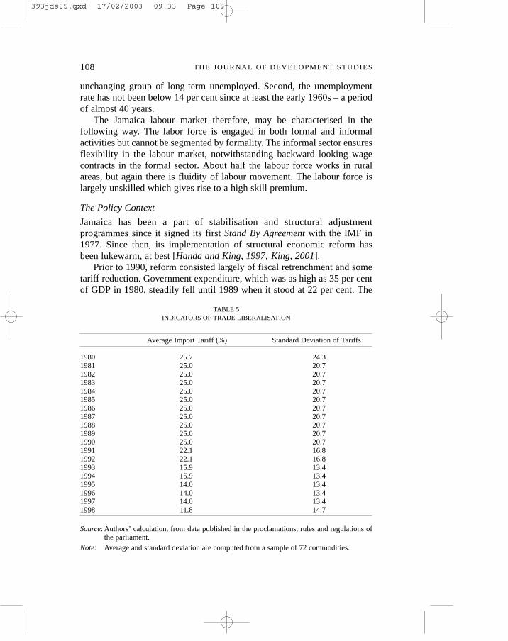
In the 1990s, current account liberalisation was implemented in earnestin several waves of tariffs reduction throughout the decade and exchangecontrols were also removed. Average tariffs had hardly changed throughoutthe 1980s since the changes in trade policy were largely in the removal ofquantitative restrictions, which only made effective the general high tariffsthat were in place. But in the 1990s, tariff rates were brought down. In 1990,the average tariff rate, computed from a representative sample of 68commodities, was 25 per cent (Table 5). The first tariff reduction exerciseoccurred in 1991 and reduced the average tariff to 22.1 per cent. Moreimportantly, the exercise started a process of simplifying the tariff code toreduce the tariff dispersion. Tariff dispersion is here measured by theestimated sample standard deviation of tariff rates, from the same sample of68 commodities. The measure fell from 20.7 to 16.8 per cent during the 1991


TABLE 6EXCHANGE RATES

Official Free Market Free Market Premium Real Exch.Rate

1980 1.8 2.5 1.40 601981 1.8 2.6 1.48 631982 1.8 2.9 1.65 611983 3.3 3.6 1.09 1001984 4.9 5.6 1.14 1201985 5.5 6.5 1.19 1121986 5.5 6.5 1.18 1021987 5.5 6.5 1.18 991988 5.5 6.7 1.22 951989 6.5 8.3 1.28 1001990 8.0 10.2 1.27 1011991 21.5 23.0 1.07 1551992 22.2 24.8 1.12 1181993 32.5 33.0 1.02 1361994 33.2 33.2 1.00 1121995 39.6 39.6 1.00 1101996 34.9 34.9 1.00 861997 36.3 36.3 1.00 841998 37.1 37.1 1.00 80

Sources: Author’s computation; Statistical Digest, Bank of Jamaica; World Currency Yearbook.‘Real Exchange Rate’ is an index measured against the United States dollar.

393jds05.qxd 17/02/2003 09:33 Page 109

round of tariff changes. The second round of liberalisation in 1993 sawaverage tariffs reduced to 15.9, and with further simplification of the tariffcode the standard deviation fell to 13.4. In 1995, another implementationdropped average tariffs to 14.0. Finally, by the last round, which was effectedin 1999, the average was brought to 11.9. Even with this, a fair amount oftrade interference still persists since the dispersion of tariffs remains high,with some tariffs, particularly those on raw materials for manufacturing, atzero, while on some final goods that compete with domestic industries, thetariff is near to and in a few cases above 100 per cent.

The liberalisation of the capital account was even more dramatic. Itbegan in 1990 when commercial banks were authorised to act as agents ofthe central bank in foreign currency transaction, which remained subject toexchange controls. Later in the year, firms were allowed hold assetsdenominated in a foreign currency in a local financial institution and toacquire foreign liabilities. In 1991, the government removed exchangecontrol restrictions on the private purchase and sale of foreign exchange,but implemented a surrender requirement of 28 per cent and imposedindicative exchange rates. Indicative exchange rates were discontinued in1993, and the surrender requirement was gradually reduced to five per centby 1995. By 1994, the premium of ‘black market’ foreign exchange thathad persisted throughout the 1980s and early 1990s had vanished (seeTable 6).

Two other elements of the policy environment that affected the macroeconomy and poverty outcomes are worth mentioning – the reversal of theeasing of the public sector burden that had been a policy achievement of the1980s and the implementation of a lengthy orthodox stabilisationprogramme to effect a disinflation. The government expenditure/GDP ratiothat had fallen as low as 22 per cent in 1989 was back to 36 per cent by1988, while the ratio of public internal debt to financial sector liabilitiesdoubled between 1991 and 1998.

Jamaica had been experiencing steady moderate inflation since the early1970s, but the inflation rate peaked at 80.2 per cent during 1991 (see Table3). The rate fell consistently from then until the end of the decade. Since thespike in the rate was due to an exchange rate shock that was accommodatedby the monetary authorities, the initial disinflation was due merely torecovery from the exchange rate shock. But in 1995, the governmentengaged an orthodox disinflation programme based on monetary targets.Whereas in the period from 1980 to 1995 the average annual growth rate ofM1 was 29.3 per cent, from 1996 to 1998 it averaged only 7.6 per cent. Thedisinflation continued through to the end of the decade.


393jds05.qxd 17/02/2003 09:33 Page 110

The Macroeconomic Context

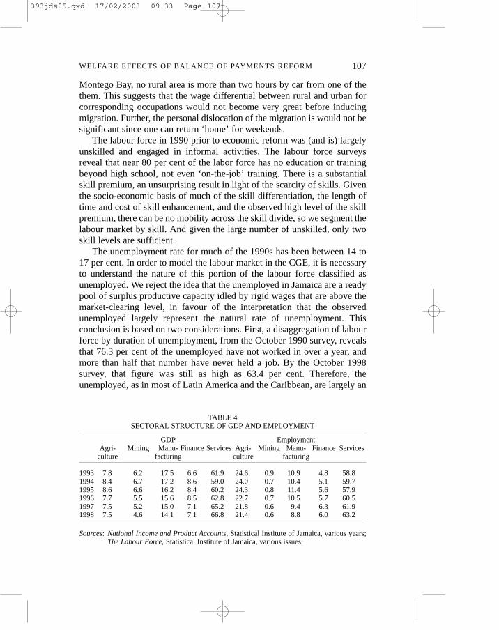
The stabilisation programme proved to be severely contractionary. Theensuing disinflation and economic contraction, in the presence of laxbanking regulation and weak capital adequacy, provoked a banking crisislater in the decade. The financial sector is relatively small, accounting foraround seven per cent of GDP and approximately six per cent ofemployment. (Table 4 shows the sectoral structure of GDP andemployment.) Therefore, any effect that financial contraction would haveon poverty and distribution would not derive from the direct effect of thatsector’s problems, but from the broader effect that the banking crisis had onthe larger economy.

The stagnation and subsequent contraction of the GDP certainly hasimplications for poverty and distribution. A declining economy would havea decreasing average income, and so to whatever extent this is spread acrossincome groups, the likelihood is that poverty should have worsened.Theoretically, the effect of GDP contraction on distribution is ambiguous,and depends on the nature of labour contracts and other rigidities in theeconomy.

The stabilisation programme itself played a large role in the evolution ofpoverty and distribution during the 1990s. Inflation and poverty are usuallycorrelated, especially in economies with labour markets characterised bybackward-looking labour contracts. The evidence from Jamaica stronglysupports this correlation. It was revealed above that between 1989 and 1992when inflation rose from 20 per cent to 80.2 per cent, the headcount for amoderate poverty line rose from 25 per cent to 32 per cent while medianconsumption fell by 11 per cent. The steady and consistent decline in therate of inflation from that peak to a rate of seven per cent in 1998 isconsistent with the steady decline in poverty.

The effect of falling inflation on distribution, however, is a lessstraightforward issue, and depends on the nature of the labour market. Itwould be expected that the formal sector, and therefore the more skilledportion of the labour force, would suffer most in an unexpected inflation,since nominal wages would be more rigid in that sector. The informal labourmarket is more flexible, so informal sector wages are less prone to laggingbehind inflation in the short run. Since skill levels are lower in the informalsegment of the labour market, the differential effects of inflation on eachlabour market segment will be evidenced in the skill premium. This isexactly what is found in the sudden rise in inflation in 1991/92. The increasein poverty was greater for relatively educated households than for theunskilled, and also greater in urban areas than in rural ones. Both of theseoutcomes corroborate the expectation that rising inflation hurts the formal,


393jds05.qxd 17/02/2003 09:33 Page 111

educated, middle class in Jamaica more relative to the informal, unskilledlower deciles.

This would account for why inequality showed such a sharpimprovement between 1989, when the Gini was 43.6, and 1991, when it was40.3. If the relationship works in the reverse, the falling rate of inflationafter 1991/92 should have produced worsening inequality. But in fact,inequality continued to decline, though not spectacularly. So disinflation, atthe very least, cannot help us to understand the fall in inequality in the1990s.

Balance of payments liberalisation is the remaining candidate to explainthe poverty and distributional outcomes. But theoretically, at least, theexpectation is ambiguous. From the liberalisation of the current account,structural realignment that may follow changes in relative sectoral priceswill in turn cause changes in returns to factors, with those changesdepending on their relative scarcity in the economy. As for the liberalisationof the capital account, the distributional impact of the increased capitalflows that usually follow such a reform are not clear. For this reason, wenow turn to a counterfactual model in order to identify the quantitative rolethat balance of payments liberalisation may have played in the socio-economic outcomes in Jamaica.

III . MACRO SIMULATIONS

The Model

In general, an economy’s response to economic reform can be temporallydisaggregated into three phases. In the first, sectors expand/contract andtherefore change their factor use in the presence of unchanged factor prices.This phase refers to the period before factor prices adjust to clear factormarkets. The second phase is the period after factor prices adjust and staticefficiency gains are therefore fully exploited. Eventually, the structure of theeconomy shifts to reflect the competitive opportunities opened up by thedynamic efficiency gains and the adoption of better production technologythat follow from structural reform. That change characterises the finalphase. The model specification was guided by a medium-run time horizon,which corresponds to the second phase of adjustment described above. Thisconsideration determined a number of assumptions.

The model is an implementation of a standard, static, Walrasian, neo-classical CGE, with structural constraints imposed in factor markets, and isbased on Robinson et al. [1999]. (The equations are available upon requestfrom the authors). The present implementation is highly aggregated. Themicro-simulations to be performed later require the estimation of earnings


393jds05.qxd 17/02/2003 09:33 Page 112

functions for each sector/labour type. Since the total number of availablehouseholds is small (Jamaica is, after all, a small country), this imposes alimit on the value of the product of sectors and labour types. In any case, forreasons which will be apparent later, the results do not seem to be sensitiveto the level of disaggregation since they derive primarily from a broadefficiency gain in the economy and not from sectoral reallocation ofresource use per se.

As a consequence, there are five productive sectors: agriculture, mining,manufacturing, finance, and other services. Mining is separated because ithas peculiar characteristics, distinct from the agricultural sector where itwould otherwise be grouped. Mining in Jamaica consists almost entirely ofbauxite extraction. There is a negligible amount of production of aggregatefor domestic construction. The mining of bauxite is highly capital intensiveand the entire output is exported. The sector uses relatively skilled labourand pays salaries that are above average for the economy. With the focus onpoverty and income distribution in the current exercise, the separatetreatment of a high wage industry is useful. Finance is also separated fromother services, again for the reason of being a relatively high wage sector.Each sector generates five commodities – imports, domestic production,domestic inputs, an absorption composite, and exports. Following theArmington process common in CGE models [Armington, 1969; Robinson etal., 1999], imports and domestic inputs are combined to produce theabsorption composite, while domestic production generates both domesticinputs and exports.

There are three factors of production – unskilled labour, skilled labour,and capital. Each factor market has unique characteristics. As is common inmodels of developing economies, capital is assumed to be fixed andimmobile and is always fully deployed, so rates of return to capital aredifferentiated across sectors (in which case, what is being collectively called‘capital’ actually represents five different, sector-specific factors ofproduction). Both types of labour are mobile, ensuring that wages in eachlabour market segment change uniformly across all sectors. The wage levelsin each production sector may differ by fixed scalars that reflect theexogenous non-wage benefits and costs of each sector.

Since we are not modeling the short run, we assume ‘nearly’ fullemployment, notwithstanding the existence of a pool of naturallyunemployed. The pool of unemployed, for a variety of reasons not explicitlymodelled, is less productive than the employed. The implication of this isthat the unemployed can be hired only at a steeply increasing cost. Themodel therefore includes wage curves for each labour market segment withunit elasticity for the unskilled segment. Skilled labour is more fullyemployed so the wage curve for that segment has an elasticity of two and a


393jds05.qxd 17/02/2003 09:33 Page 113

smaller pool of naturally unemployed. Inflationary expectations are static,so nominal wage changes are influenced only by the state of the labourmarket, not by concurrent changes in the general price level.

The model does not contain an explicit monetary module. There is nointerest rate, apart from the return to capital, and no explicit credit market,apart from the savings-investment identity. The implicit monetaryinstrument is therefore the numeraire, which is the nominal exchange rate.

The model is not dynamic and does not include any means of increasingproductive capacity, either from changes in the capital stock or othersources. While employment may increase, the labour force does not grow.In this sense, the model (like all static CGEs) has no capacity for generatinggrowth, in the sense of an expanded GDP based on a greater productivecapacity. Growth outcomes presented below are therefore to be interpretedas representing a change in GDP above or below whatever would haveotherwise been produced by the underlying growth forces in operation.

The characterisation as Walrasion means that market clearing for allcommodity markets is implicit and all market prices and quantities aredetermined endogenously, except for the import good being in perfectlyelastic supply and the export good being in perfectly elastic demand, eachat their prevailing world price. This is the ‘small country’ assumption.

This neoclassical CGE model, or following Robinson [1989], an‘elasticity structuralist’ model, uses a savings-driven closure. That is, we donot assume that there is a savings or foreign exchange gap which constrainsinvestment. This assumption is made to reflect the characteristics of theJamaican economy. Jamaica has employed a market determined exchangerate at least since 1993 (and arguably, even before that during the period ofexchange controls and an ‘official’ exchange rate), with a target level offoreign reserves (notwithstanding occasional short term interventions).Moreover, the crux of macro policy has been an orthodox, inflation-targeting monetary policy. For this reason, it is important to be able to holdmonetary policy constant by making it explicit, and this argues for beingable to choose the nominal exchange rate or the domestic price level as thenumeraire, so that it may remain exogenously unchanged. Given theexogeniety of foreign savings required by the presence of a market-determined exchange rate, an investment-driven specification would haverequired that monetary policy be implicit.

The sectoral composition of private consumption, investment andgovernment demand are in fixed proportions, as is the division ofgovernment expenditure between government consumption of product andwages. The model’s parameters are calibrated to the 1993 national accounts.The SAM is aggregated from a 34-sector one computed by the PlanningInstitute of Jamaica.


393jds05.qxd 17/02/2003 09:33 Page 114

Balance of Payments Liberalisation Scenarios

In light of the liberalisation of current and capital account transactions inJamaica between 1989 and 1998, three policy actions are simulated usingthe model: current account liberalisation only, capital account liberalisationonly, and a combination of both.

Current account liberalisation is simulated by means of an across-the-board tariff reduction, using the single import tariff as the instrument.Between 1993, the base year for this analysis, and 1998, the average tariffrate declined by 46.6 per cent, so this is the amount of the reduction that isapplied to the base year tariff in each of the five sectors. Tariff reform alsotook the form of a reduction of the tariff dispersion, but no attempt is madeto model this element of the policy environment.

The second exercise represents capital account liberalisation. Capitalaccount liberalisation presents a greater challenge to the modeler since itrepresents a change in the way the market operates, which would in turnrequire a re-specification of the model. While the model can be changed toreflect the altered manner in which external transactions are conducted, thisdoes not provide a means by which to measure quantitatively the effect ofsuch a change. The usual procedure is to model capital accountliberalisation in terms of its main observable effect, namely, an increasedinflow of foreign capital. This is inadequate for a two reasons. First, theremoval of restrictions on external capital flows may have a number ofprimary effects, of which higher capital inflows is only one. By focusingonly on higher capital inflows, these other primary effects and allconsequences that follow from them will be ignored. Second, liberalisationof the capital account will have sectorally differentiated effects that are notcaptured by using only the instrument of increased capital inflows. Since ageneral equilibrium model is a multi-sector methodology, the omission ofsectoral effects is an unnecessary one.

A different approach is taken here. Our interest is the effect of capitalcontrols on current transactions. Exchange controls impose a cost on currentaccount transactions by forcing a rationing of limited foreign exchange.This cost derives from the rent-seeking behaviour induced by the ration andfrom the risk incurred in evasion. Accordingly, the cost of capital accountrestrictions are represented in the model by an obligation to use a ‘rent-seeking’ commodity in production, along with the usual intermediates andvalue added. Firms buy imported intermediates using rationed foreignexchange, but also buy the rent-seeking premium that is necessary in orderto acquire the foreign exchange. We assume that rent-seeking is ‘produced’just like any other commodity, and is supplied by a specialised industry. Theproduction of rent-seeking, being a directly unproductive activity, is treated


393jds05.qxd 17/02/2003 09:33 Page 115

as an intermediate product rather than as final demand. In the specification,the rent-seeking requirement is an additional element in the intermediateinput vector for each activity. It is therefore a diversion of productiveresources away from uses that directly or indirectly could add to welfare.Our treatment of capital account restrictions is accomplished therefore, inessence, by introducing a dead-weight loss into production.

For the present purpose, this is a more appropriate treatment than anexogenous jump in capital inflows since this treatment recognises that rent-seeking not only has a redistributive effect amongst the sectors, but alsoimposes a cost on production activities. There is ample empirical evidencethat rent-seekers are willing to incur considerable costs to secure economicprivileges. Deacon and Sonstelie [1989] provide evidence of the willingnessof buyers to incur costs in order to procure price controlled, rationedcommodities in developing countries. Thorbecke [1993] has argued thatthese rent-seeking costs far exceed the dead-weight losses of tradeprotection per se. Beck and Connolly [1996] conclude that for Canadianfirms over a 12-year period, rents were completely dissipated.

This treatment is similar but not identical to the use of rent-seeking torepresent quantitative restrictions on imports in a model of Turkey in Grais,de Melo and Urata [1986]. The present treatment departs from thatimplementation in the assumptions made in regard to the production anddistribution of the rent-seeking activity. While Grais et al. assume thatproduction of rent-seeking reflects the production technology of the activityusing rent-seeking, the assumption in the present model is that there is a singleproduction process for rent-seeking which is carried out by the service sectorusing the production technology of services and bought by all users. Theearnings from rent-seeking therefore accrue entirely to the service sector.

This assumption seems more suitable than that of Grais et al., becausein the present case, all users are vying for the acquisition of a single rationedcommodity (hard currency) and therefore participating in the same marketfor that commodity. In Grais et al., since the ration applies separately toeach imported commodity, there are many separated rent-seeking activities,and therefore different prices. Further, many firms outsourced theacquisition of black market dollars to freelance traders, the producers ofrent-seeking, suggesting that rent-seeking was performed in a homogenoussector.

Grosse [1994], in his discussion of the black market for foreign exchangein Jamaica in the 1980s, indicates that it was characterised by numerousintermediaries at both the wholesale and retail levels. He further points outthat the number of dealers in large transactions was larger than obtained inLatin American economies that also had parallel currency markets. Thetypical dealer, according Grosse, would operate a legitimate foreign-


393jds05.qxd 17/02/2003 09:33 Page 116

exchange related business officially, while trading in black market dollars inthe ‘backroom’. In his article on the black market in Columbia, Gross [1992],points out that it, too, was conducted by an industry of intermediaries,cambistas, who were often legitimate financial dealers at the same time.Both the development of specialised intermediaries and the observation thatmany were in the finance industry suggest that black market currency tradingshould be modelled as sharing the technology of other financial activity,rather than that of the sector of the firm buying the foreign exchange.

In our model, neither consumers nor the government, by assumption,directly buy rent-seeking. The government does not participate in theforeign exchange ration, enjoying first call on available foreign exchange,and consumers purchase imports only through the intermediation ofdomestic activities. Firms will incur the cost of rent-seeking in directproportion to the amount of imported intermediates they require, scaled bythe premium factor.

Following Edwards and Khan [1985], the premium on the exchange ratein the black market is used as a proxy for the severity of capital controls andas an estimate of value of the consequential rent-seeking. The liberalisationof the capital account can therefore be simulated by a reduction in the rateof the premium. In 1993, the black market exchange rate premium stood at12 per cent, coming down from an average of 22 per cent in the latter halfof the 1980s (Table 6). By 1995, the premium had been eliminated. Thus, inthe base run simulation, the premium is set at 12 per cent. Capital accountliberalisation is simulated by a reduction of this rate to zero.

The third simulation is a combination of the two exercises above. SinceCGE models are non-linear, the combination yields results that are notnecessarily equal to the mere summation of the separate effects.

As with all similar analyses using CGE’s, only a limited range of theeconomy’s responses to policy change is reflected in the results provided.The assumptions that have guided the specification and assumptions of thepresent exercise are those most consistent with the objective of capturingonly the medium run of adjustment. Accordingly, there is much in theresponse of the economy to trade and payments liberalisation not capturedin the simulations below, and therefore elements of the effects on povertyand income distribution not included.

Simulation Results

The first exercise simulates the liberalisation of the current account bymeans of a reduction of almost half in tariffs, applied uniformly across allsectors. The results appear in the second and fifth data columns of Table 7,with the base year (simulated) values in the first column. Themacroeconomic impact of the tariff reduction is negligible. GDP remains


393jds05.qxd 17/02/2003 09:33 Page 117


TABLE 7SIMULATED MACRO AND LABOUR MARKET OUTCOMES OF BOP REFORMS

Levels % ChangeBase C Acc. K Acc. BOP C Acc. K Acc. BOP

MACROECONOMY

Broad IndicatorsGDP 100.00 100.01 110.26 110.33 0.0 10.3 10.3Imports 96.39 96.92 99.64 100.38 0.6 3.4 4.1Exports 47.82 48.27 50.59 51.22 0.9 5.8 7.1Fiscal Balance 1.35 -0.37 2.58 0.82 -127.6 90.3 -39.2Ret to K 1.00 1.01 1.04 1.05 0.7 4.3 5.4CPI 1.00 0.99 0.93 0.92 -1.4 -7.1 -8.4Real Exch. Rate 1.00 1.02 1.11 1.13 2.0 10.5 12.7Unemployment 0.04 0.04 0.04 0.04 -0.1 -0.5 -0.8

Sectoral OutputAgriculture 18.65 18.75 19.25 19.34 0.6 3.2 3.7Mining 18.38 18.40 18.47 18.49 0.1 0.5 0.6Manufacturing 43.22 44.01 48.74 49.80 1.8 12.8 15.2Finance 10.24 10.26 10.38 10.42 0.2 1.4 1.7Services 94.50 93.86 90.38 89.65 -0.7 -4.4 -5.1

Sectoral PricesAgriculture 1.00 1.00 1.00 1.01 0.0 0.5 0.7Mining 1.00 1.00 1.00 1.00 0.1 -0.1 -0.1Manufacturing 1.00 0.99 0.96 0.95 -0.9 -4.4 -5.1Finance 1.00 0.99 0.97 0.96 -0.6 -3.4 -3.8Services 1.00 0.99 0.95 0.94 -0.9 -5.1 -5.9

LABOUR MARKET

UnskilledAgriculture 31.76 32.17 34.18 34.57 1.3 7.6 8.8Mining 0.74 0.75 0.76 0.77 0.6 2.7 3.0Manufacturing 9.04 9.23 10.41 10.67 2.1 15.1 18.1Finance 0.84 0.84 0.84 0.84 0.0 0.3 0.5Services 52.47 51.87 48.69 48.05 -1.2 -7.2 -8.4Unemployed 5.15 5.14 5.12 5.10 -0.1 -0.5 -0.9

SkilledAgriculture 8.86 9.01 9.76 9.90 1.7 10.1 11.8Mining 1.07 1.08 1.13 1.13 1.0 5.1 5.8Manufacturing 14.50 14.87 17.09 17.59 2.5 17.8 21.3Finance 2.66 2.67 2.73 2.74 0.4 2.7 3.2Services 71.91 71.37 68.29 67.62 -0.8 -5.0 -6.0Unemployed 0.99 1.00 1.00 1.00 0.1 0.9 0.9

WagesUnskilled 1.00 1.00 1.01 1.01 0.1 0.6 0.9Skilled 1.52 1.51 1.49 1.49 -0.3 -1.7 -1.7Skill Premium 1.52 1.51 1.48 1.48 -0.4 -2.3 -2.6

393jds05.qxd 17/02/2003 09:33 Page 118

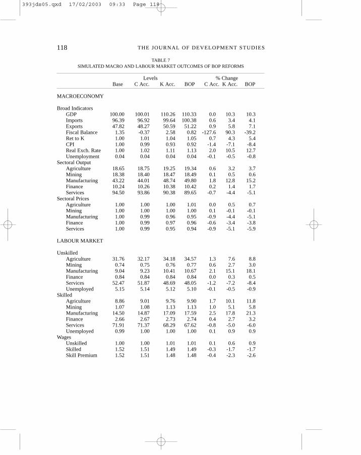
unchanged, with negligible increases in both imports and exports. With nochange in GDP, unemployment remains at its base level. As would beexpected, the fiscal accounts deteriorate somewhat, by about two per cent ofGDP in the absence of compensating revenue generation to offset therevenue loss due to lower import tariffs. The initial surplus of 1.4 per centof GDP turns into a deficit of 0.4 per cent.

Prices fall somewhat (by two per cent) directly as a result of the tariffreduction, which (given that the exchange rate is the numeraire) isequivalent to a real depreciation. The tariff reduction, because it lowersdomestic currency import prices, raises the demand for imports and foreignexchange. Wages in both labour market segments and returns to capitalremain virtually unchanged in real (international) terms.

The sectoral adjustment that follows from the current accountliberalisation is not quantitatively significant. Outside of a two per centexpansion in manufacturing, output changes in no other sector by more thanone per cent. On the basis of this simulation, very little effect on poverty andincome distribution can be expected from the tariff reduction since there islittle effect on the relative sectoral magnitudes and the macroeconomicaggregates. This simulation result corroborates the observation that Stolper-Samuelson effects have been empirically inconsequential in developingcountries in the medium run.

The results for the simulated liberalisation of the capital account arepresented in the third and sixth data columns of Table 7. The GDP expandsby an impressive 10.3 per cent. Given the estimated time horizon of aboutfive years for the exercise simulated here, this suggests that capital accountliberalisation by itself may add about two percentage points to the growthrate over the medium run. The growth of final goods output arises from theredeployment of factors freed from the obligation to produce theintermediate service, rent-seeking. Since we assume relatively steep wagecurves, the result is not unemployment of factors but expansion of theproduct of the remainder of the economy. This is an efficiency gain, similarto that which might be obtained from a technological improvement.

Both exports and imports rise in this scenario, by 5.8 per cent and 3.4per cent respectively. Imports rise since their relative price falls with theremoval of the ‘tax’ of rent-seeking and exports rise to restore fullabsorption of the productive capacity. There is a real depreciation of 10.5per cent to reflect the fall in domestics costs. The fiscal balance improveson the basis of the revenues from the macroeconomic expansion.Employment increases by just under two per cent, but wages and the returnto capital rise significantly. This is in keeping with the greater demand foroutput in the presence of relatively full employment.

The liberalisation of capital flows also has consequences for sectoral


393jds05.qxd 17/02/2003 09:33 Page 119

adjustment and labour use. Changes to the sectoral distribution of output isdominated by the removal of the obligation to buy rent-seeking from theservice sector. As a result, the service sector shrinks by 4.4 per cent and itsprice falls by five per cent. This contraction frees up labour (but not capitalwhich is not mobile) to shift to other sectors. These other sectors will takeadvantage of the freed up capacity to the extent to which they benefit fromthe reduction in import prices, which is determined by their import content.Manufacturing has the largest import content, so its price falls by 4.4 percent and production expands by 12.8 per cent.

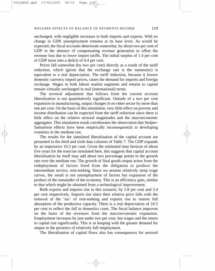
The outcomes that are most likely to affect poverty and incomedistribution are changes to the structure of wages amongst skills and oflabour use amongst sectors. The labour market response reflects the sectoralchanges. The service sector is, by multiples, the largest user of skilledlabour, so the service sector contraction depresses the demand for and thereturn to skilled labour. Thus, the skill premium falls, though by only twoper cent. All other sectors increase their use of the labour released byservices, with the manufacturing sector absorbing the most. Much of theunskilled labour is absorbed by the agricultural sector, which provides thebasis for a modest expansion (by 3.2 per cent) of that activity.

The distributional effects investigated below are confined to thedistribution of labour income, but it is noteworthy that return to capital risesby 4.3 per cent. This arises from the increased demand for factors toproduce the expansion, while capital is not free to shift out of thecontracting sector due to the assumption of immobile capital.

When both current and capital account reform is combined, themacroeconomic outcome and microeconomic adjustment reflect thedominance of the effect of capital account liberalisation. Results for thissimulation are presented in columns four and seven of Table 7. Theexpansion of GDP reflects the effect of the liberalisation of the capitalaccount, as does the increase in international trade, but the increase is nowgreater because of the additional effect of tariff reduction. In addition, thereal depreciation and the rise in the return to capital correspond to the


TABLE 8RANKING OF SECTORS (INITIAL LABOUR MARKET SHARES)

Skilled Unskilled

Finance (2.57) Finance (0.83)Mining (1.05) Mining (0.73)Services (69.28) Services (51.73)Manufacturing (14.14) Manufacturing (8.88)Agriculture (8.53) Unemployed/Other (6.60)Unemployed/Other (4.44) Agriculture (31.23)

393jds05.qxd 17/02/2003 09:33 Page 120

simulation of capital account reform only, again with slightly largermagnitudes because of its combination with the effect of a tariff reduction.

Sectoral adjustment also largely reflects the outcome of the capitalaccount reform. The service sector contracts while manufacturing and to alesser extent agriculture expand. Skilled and unskilled labour use shiftsaccordingly and the skill premium falls.

From the above simulations, the outcomes that matter for thedistribution of labour income are the reallocation of labour amongst sectorsand of returns amongst skill levels. The reallocation of labour amongstskills levels will affect the distribution because all sectors do not pay thesame wage, and so the shift of labour from services to manufacturing andagriculture will affect the incomes of the households that change sectors.The aggregate distributional effect is an empirical matter. The householdsshifting from services to finance will enjoy a rise in household income whilethose moving to manufacturing and agriculture (the vast majority in thiscase) will suffer a fall in household income. This might suggest a rise inpoverty and a worsening of the distribution. At the same time, the incomeof the skilled has fallen relative to the unskilled while there has been a smallrise in the wage rate of the unskilled, which implies a reduction of povertyand an improvement of the distribution. The empirical sorting out isaccomplished by the household level simulations explained below.

IV. MACRO TO MICRO: THE DISTRIBUTIONAL IMPACT

Methodology

The CGE simulations discussed above provide new labour market profilesor outcomes (LMP) which we translate into changes in household welfare;we make the link between the CGE and household welfare using the SLC.The predicted LMP is mapped into the SLC using the sector of employmentand skill level of the principal earner of the household, grouping theseprincipal earners into the same 12 categories as those generated by the CGE– five production activities plus unemployment for both the skilled and theunskilled. Thus, households in the SLC are assigned to sectors based on theemployment sector of the principal earner, as reported by households in thesurvey, and household welfare is measured using total household per capitaconsumption, consistent with the poverty profile.

For this exercise we use both the 1993 and 1994 rounds of the SLC inorder to have sufficient households within each sector of employment. Wedo not combine all rounds of the SLC because there are fluctuations inoverall welfare from year to year due to, for example, macroeconomicconditions, and we do not want these to interfere with the results from the


393jds05.qxd 17/02/2003 09:33 Page 121

policy simulations. We choose 1993 and 1994 since these are two adjacentand relatively similar years in terms of welfare outcomes; note that the CGEmodel’s parameters are calibrated using 1993 data.

The CGE simulations provide hypothetical labour market shares foreach sector, which we subsequently impose on the households in the SLC.Using these new sector shares we calculate poverty and inequality measuresin order to assess the ‘impact’ of the macroeconomic policy change onwelfare outcomes. To go from the existing sectoral distribution of the labourforce (and its associated welfare distribution) to the hypothetical one (fromwhich we compute the new welfare distribution) we must makeassumptions about the inter-sectoral mobility of households. We modelhousehold mobility in the following way. First, we sort households bysector, with households in the sector with the highest mean welfare at thetop, followed by households in the sector with the next highest level ofwelfare, and so on. Within each sector, however, households are sortedrandomly.

Each simulation of the CGE yields a new labour market profile,consisting of the shares in each sector. We assign households to new sectorsby starting from the top, and assigning households to finance, mining,manufacturing, and so on, with the exact number of households chosen inorder to attain the new sectoral share as dictated by the result of the CGEsimulation. For example, if there were 100 households in the sample, andthe CGE simulation predicted a new labour market share of ten per cent inthe financial sector and five per cent in mining, then the first ten householdswould be assigned to the financial sector, the next five to mining, and so on.

We highlight three important points about this methodology. First, theordering of sectors is carried out separately for skilled and unskilledhouseholds.2 In the micro-simulations we therefore divide households intotwo groups, those whose principal earners are skilled, and those whoseprincipal earners are unskilled, and the micro-simulation is done separatelyfor these two groups (hence, workers who are ‘unskilled’ cannot move tothe ‘skilled’ sector); the resulting sub-distributions are combined tocalculate the overall change in welfare in the sample. Second, householdscan generally only move into an adjacent sector. And lastly, becausehouseholds are sorted randomly within each sector, households who moveto an adjacent sector may not necessarily be the richest or poorest.

Once we have established a mechanism to generate household mobilitybetween sectors, we must find a way a plausible way of deriving the newwelfare distribution, which we do by estimating sector specific householdwelfare coefficients. That is, for households in each sector, we carry out anOLS regression relating household characteristics to (the log of) totalconsumption. The household characteristics include region of residence,


393jds05.qxd 17/02/2003 09:33 Page 122


TABLE 9DETERMINANTS OF LOG PER CAPITA HOUSEHOLD CONSUMPTION BY SECTOR

Agriculture Mining Manufac. Finance Services Other

Heads DemographicsFemale headed Hhold -0.127 -0.553 -0.243 0.171 -0.120 0.075

(2.97) (1.18) (3.12) (0.50) (3.86) (0.66)Age of head in years 0.000 0.153 0.032 0.111 0.017 0.036

(0.02) (1.30) (1.84) (2.10) (2.73) (1.79)Head’s age squared 0.000 -0.002 0.000 -0.001 0.000 0.000

(0.88) (1.25) (1.88) (2.14) (3.46) (2.09)Head has partner in hhold -0.116 -0.088 -0.090 0.507 0.026 0.188

(2.28) (0.15) (1.08) (1.56) (0.80) (1.07)Head’s SchoolingNone -0.143 0.775 0.590 0.882 0.471 -0.205

(1.51) (1.36) (3.17) (1.69) (9.22) (0.70)Some primary -0.086 0.000 -0.223 0.366 -0.152 -0.392

(1.79) (0.00) (1.53) (0.48) (2.83) (2.71)Grade 9 -0.024 0.770 -0.050 0.487 0.095 0.115

(0.53) (2.26) (0.55) (0.88) (2.75) (0.81)Grade 11 0.182 1.051 0.070 0.654 0.251 0.296

(2.23) (1.97) (0.65) (1.17) (6.02) (1.49)A level or more 0.424 1.372 0.405 0.889 0.566 0.230

(2.02) (2.90) (2.66) (1.71) (9.53) (1.06)Rural -0.085 0.744 -0.166 -0.250 -0.212 -0.268

(0.76) (0.65) (2.31) (0.77) (7.39) (2.59)Town -0.076 0.671 -0.148 -0.467 -0.203 -0.108

(0.62) (0.55) (1.85) (1.52) (6.63) (0.78)Household Demographics

Ln(Household size) -0.533 -1.008 -0.644 0.252 -0.573 0.081(8.08) (1.21) (5.32) (0.36) (12.14) (0.33)

Residents 0–5 -0.060 0.243 -0.120 -0.419 -0.088 -0.376(2.10) (0.74) (2.17) (1.33) (4.77) (3.02)

Residents 6–14 -0.013 0.177 -0.015 -0.047 -0.027 -0.232(0.55) (0.66) (0.36) (0.19) (1.60) (2.27)

Males 15–19 -0.001 -0.203 0.019 -0.034 0.003 -0.213(0.04) (0.46) (0.25) (0.07) (0.11) (1.28)

Females 15–19 0.068 0.091 0.157 -0.601 0.035 0.108(1.55) (0.12) (2.28) (1.03) (1.20) (0.52)

Males 20–29 0.090 0.651 0.096 0.181 0.117 0.129(2.58) (2.10) (1.61) (0.45) (4.89) (0.48)

Females 20–29 0.123 -0.006 0.223 -0.220 0.130 -0.163(2.91) (0.01) (3.18) (0.83) (4.88) (0.92)

Males 30–39 0.193 0.160 0.194 -0.919 0.156 -0.009(3.95) (0.31) (2.42) (1.85) (4.69) (0.03)

Females 30–39 0.308 -0.172 0.344 -0.059 0.204 -0.079(5.52) (0.31) (3.61) (0.16) (5.81) (0.38)

Males 40–49 0.182 1.428 0.087 -0.415 0.195 -0.021(3.17) (0.88) (0.81) (0.48) (4.65) (0.05)

Females 40–49 0.302 0.105 0.248 -0.424 0.153 -0.143(4.32) (0.14) (2.12) (0.70) (3.49) (0.41)

Males 50–64 0.111 1.325 0.136 0.050 0.083 -0.276(1.87) (0.84) (1.23) (0.09) (1.76) (1.10)

Females 50–64 0.216 0.684 0.006 -0.817 0.174 -0.110(3.48) (0.57) (0.05) (1.56) (3.92) (0.55)

Residents 65 and over 0.128 3.334 0.064 -0.154 0.088 -0.227(2.40) (1.32) (0.63) (0.32) (2.30) (1.38)

Constant 10.370 6.424 10.021 8.005 10.290 9.628(45.22) (2.38) (25.51) (5.63) (69.05) (17.92)

Observations 1018 31 390 47 2154 238R-squared 0.34 0.93 0.43 0.72 0.42 0.30

Note: ‘Sector’ is that of principal earner. Absolute value of t-statistics in parentheses. Excluded category ismale head with no resident partner, complete primary school education, and residing in Kingston.Data are 1993 and 1994 SLC combined.

393jds05.qxd 17/02/2003 09:33 Page 123

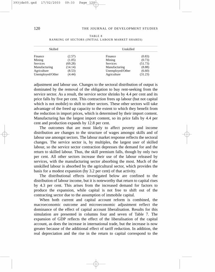
sex, age and schooling of head, demographic composition, and (the log of)household size. Using these coefficient estimates, we predict theconsumption that each household would have, given its characteristics, if itmoved to another sector. Thus, for each household, we have an estimate ofits consumption (welfare) if it moved to another sector based on sectorspecific regression coefficients and its existing characteristics, and of coursewe have its actual welfare in its current sector. However, for the new welfaredistribution we use predicted consumption for all households, whether thehousehold stays in its original sector or moves to a new sector. This is doneto maintain comparability, as the distribution of predicted consumption willhave less variance around the mean, relative to actual consumption.

The CGE simulations also provide estimates of changes in the real wagein the economy, which we also account for in the consumption estimation.Real wage changes are unlikely to translate into equal changes in householdconsumption for two reasons. First, the marginal propensity to consume outof cash income is not unity. Second, not all of household income may derivefrom wage income. For these reasons, each per centage change in the realwage is assumed to translate into a 0.5 per cent change in total householdconsumption.

Once all households have been reassigned and estimated householdconsumption computed, hypothetical poverty outcomes (populationweighted) can be calculated. For the simulated scenario, each household’swelfare is determined by its predicted consumption for the sector in whichit works, conditional upon its household characteristics.

There are two important methodological issues to note. First, overallwelfare will depend on the extent to which better paying sectors (such asfinance, mining, and manufacturing) expand while worse paying sectorscontract. Second, overall welfare will also be determined by the type ofhouseholds that are randomly assigned to switch sectors. Becausehouseholds are chosen randomly to move between sectors, those who move‘up’ to better sectors may not necessarily be the richest households in theoriginal sector. Similarly, households who move ‘down’ are not necessarilythe poorest households in the original sector.3 Because the new povertyindicators are partly based on random selection, we ‘bootstrap’ eachsimulation. That is to say, for each new simulated LMP, we calculate thenew welfare distribution 20 times, each calculation based on a new randomselection of the particular households to move from each sector. Wecalculate the mean (and related statistics) over these 20 simulations andpresent this as a more reliable poverty estimate for any givenmacroeconomic policy simulation.


393jds05.qxd 17/02/2003 09:33 Page 124

Poverty Implications of Policy Simulations

Table 9 presents the full OLS regression results for the sector specificdeterminants of household consumption, measured in log terms. These arethe coefficients used to predict hypothetical consumption if a householdwere to move into these sectors. (Actual predicted welfare is the antilog ofthe predicted value of the dependent variable in these regressions.)

Using the methodology described above, we calculate four povertyindicators for each policy simulation: (1) headcount using a relative 25 percent ‘moderate’ poverty line; (2) poverty gap using the relative 25 per centpoverty line; (3) headcount using a relative ten per cent ‘extreme’ povertyline; (4) mean per capita household consumption. For each indicator, wepresent the percentage change in its value relative to the original value,where the original value is calculated using the actual distribution ofpredicted consumption from the combined sample of SLC 93 and 94 (allunits deflated to 1993 Jamaican dollars).

Summary statistics based on the results of the household simulations areprovided in Table 10. For each policy we present two simulations, one thatonly takes into account the wage change evoked by the policy, and thesecond that considers both the wage and labour market structure changes. Inthe case of wage changes only, there is no randomness involved in the


TABLE 10CHANGE IN POVERTY/DISTRIBUTION INDICATORS DUE TO POLICY

SIMULATIONS – WAGE AND ACCUMULATED EFFECTS (PERCENTAGE CHANGE)

Wage Only Accumulated ImpactMean St. Dev. Minimum Maximum

Current AccountHeadcount (25% Line) -0.423 -0.345 0.114 -0.587 -0.123Poverty gap (25% Line) -0.413 -0.309 0.242 -0.694 0.293Headcount (10% Line) -1.037 -0.829 0.261 -1.173 -0.286Mean Consumption 0.058 3.606 13.373 0.003 59.290Gini Coefficient -0.457 -0.429 0.092 -0.509 -0.187Capital AccountHeadcount (25% Line) -1.760 -0.184 0.625 -1.214 0.914Poverty gap (25% Line) -2.344 -1.003 0.975 -2.668 0.935Headcount (10% Line) -3.356 -2.203 1.335 -4.515 0.805Mean Consumption 0.245 0.732 2.958 -0.164 13.150Gini Coefficient -0.845 -0.409 0.636 -0.906 2.067BothHeadcount (25% Line) -1.760 -0.140 0.539 -1.241 0.778Poverty gap (25% Line) -2.344 -0.769 1.244 -3.437 2.188Headcount (10% Line) -3.356 -2.121 1.388 -4.924 0.532Mean Consumption 0.245 0.175 0.563 -0.266 1.849Gini Coefficient -0.845 -0.391 0.321 -0.695 0.824

Note: Accumulated effect refers to both wage and labour market simulation combined.

393jds05.qxd 17/02/2003 09:33 Page 125

simulation and so the simulation is run only once, and this is the resultshown in the first column of the table.

The results from the current account simulations which only considerwage effects show a small decline in poverty for all three indicators, withthe largest decline (1.04 per cent) occurring for the ten per cent severepoverty line. The accumulated effect also results in small declines inpoverty and inequality, and again, the largest decline is for the ten per centextreme poverty headcount (0.83 per cent). Although this latter effect issmall, its standard deviation is much smaller, so that both minimum andmaximum values are negative.

On the other hand, the capital account policy simulation delivers a largerincrease in mean consumption, and correspondingly bigger changes inpoverty outcomes, but mostly driven by wage changes. The wage-onlysimulations show reductions of 3.4 per cent reduction in severe poverty and1.8 per cent in moderate poverty. The full simulation including both wageand sectoral effects show mean reductions of 2.2 and 0.2 per cent in thesevere and moderate povertly line headcount respectively. However thestandard deviation of these mean responses are larger in this scenario, so thatthe two standard deviation interval around the means always contains 0.

The simulations that liberalise both current and capital accounts deliverwelfare changes along the lines of the capital account simulations. In thiscase as well, the primary cause of the improvement in welfare comes fromwage effects rather than shifts in the sectoral allocation of labour. Noticethat the wage only effects are identical to those of the capital accountliberalisation simulation since both policies deliver the exact same wageeffects in the CGE model. Furthermore, the poorest seem to benefit themost, as witnessed by higher percentage declines in the moderate povertygap (0.8) and the severe poverty line headcount ratio (2.1). However inthese simulations as well, the standard deviations are large relative to thecalculated mean changes, so that again, the two standard deviation intervalaround the mean responses always includes 0.

CONCLUSION

The first noteworthy result in this study is the large magnitude of themacroeconomic effect of capital account liberalisation. This hasmethodological importance since that policy change is modeled here in aunique way, namely, by setting up a specialised rent-seeking activity. Theresult also has broad policy implications. It suggests that the dead weightloss imposed on economies by capital account restrictions may bequantitatively significant, more than ten per cent of GDP in the presentexample, and may be larger than the effects due simply to sectoral


393jds05.qxd 17/02/2003 09:33 Page 126

misallocation. Finally, the results suggest that the static welfare gain ofcapital account reform is more important than that of trade reform, whichturns out to be negligable. This derives from the fact that the static cost ofhigh tariffs accrue to another agent in the economy, the government, whosedisposal of that wealth may offset the welfare loss of the import tax. In otherwords, the rent-seeking tax is a dead-weight loss while the import tax isonly a reallocation.

Taken as a whole, the results indicate that balance of paymentsliberalisation will have a positive effect on the economic welfare of thepoor, although the extent of the impact depends on the type of policyimplemented. By far the ‘best’ policy from a poverty standpoint is capitalaccount liberalisation. The simulations indicate that the extreme poor arelikely to benefit from this policy. Current account liberalisation, on the otherhand, delivers smaller declines in poverty, although in this scenario as well,it is the extremely poor who are likely to benefit the most. Finally,liberalising both capital and current accounts would lead to improvementsin welfare along the lines of capital account liberalisation alone, accordingto the simulation results and methodology presented in this article. In thesetwo scenarios (capital account liberalisation and full balance of paymentsliberalisation), the largest gains in welfare come about from wage changesrather than movement in the sectoral allocation of labour.

The small magnitudes of the changes in the poverty and distributionmeasures is striking, especially in the presence of a significant (ten per cent)change in GDP. The largest effect is a 2.2 per cent decline in the incidenceof severe poverty. The result is consistent with empirical observation ofpoverty and distributional changes in Latin America and the Caribbean overthe last two decades of substantial economic reform. It is worthremembering that the results above apply only to the medium-run effect ofthe policy change. No attempt is made to simulate the long run growthbenefit that would derive from a more competitive economy following tradeand exchange liberalisation, which is their substantive justification. Thosewill have entirely different distributional consequences.

In the case of Jamaica, the results imply that trade and payments reformmay partly account for the observed poverty and distribution outcomes inthe 1990s. Declining inflation may not be the only factor at work inaccounting for declining poverty in the context of a stagnating economy.Reallocation of productive resources away from uses that do not contributeto welfare may have played a role as well.

final revision accepted February 2002


393jds05.qxd 17/02/2003 09:33 Page 127

NOTES

1. This is a direct consequence of the ample supply of public primary schooling which gives almosteveryone the opportunity to finish primary and middle school, but which is of poor quality, sothat completion of primary or middle school does not necessarily lead to higher productivity orincome.

2. The poverty profile indicates that completing grade 11 is a key factor in escaping poverty, andso we define principal earners with grade 11 or more schooling as being skilled.

3. An alternative would be to specify a ‘moving’ function to predict exactly which households arelikely to move. However we have no firm basis for specifiying such a function, and so randomlyassign households to move. Note that within our set-up, households can only move to adjacentsectors.

REFERENCES

Armington, Paul 1969, ‘A Theory of Demand for Products Distinguished by Place of Production’,Staff Papers, Vol.16, No.1.

Beck, R.L. and J.M. Connolly 1996, ‘Some Empirical Evidence on Rent-Seeking’, Public Choice,Vol.87, Nos.1–2.

Boyd, Derick 1987, ‘The Impact of Adjustment Policies on Vulnerable Groups: The Case of Jamaica,1973–85’, in Giovanni Cornea, Richard Jolly and Frances Stewart, Adjustment with a HumanFace, Vol.2, New York: UNICEF.

Deacon, Robert T. and Jon Sonstelie 1989, ‘Price Controls and Rent-Seeking Behavior in DevelopingCountries’, World Development, Vol.17, No.2.

Edwards, Sebastian, and Mohsin S. Khan 1985, ‘Interest Rate Determination in DevelopingCountries: A Conceptual Framework’, Staff Papers, Vol.32, No.3.

Gafar, John 1997, ‘Structural Adjustment and the Labour Market in Jamaica’, Canadian Journal ofDevelopment Studies, Vol.XVIII, No.2.

Gallimore, Courtney L. 1996, ‘A Computable General Equilibrium (CGE) Model of Jamaica’,mimeo, Planning Institute of Jamaica, Kingston, Jamaica.

Grais, Wafik, de Melo, Jaime and Shujiro Urata 1986, ‘A General Equilibrium Estimation of theEffects of Reductions in Tariffs and Quantitative Restrictions in Turkey in 1978’, in T.N.Srinavasan and John Walley (eds.), General Equilibrium Trade Policy Modeling, Cambridge,MA: MIT Press.

Grosse, Robert, 1992, ‘Columbia’s Black Market in Foreign Exchange’, World Development, Vol.20, No.8.

Grosse, Robert, 1994, ‘Jamaica’s Foreign Exchange Black Market’, The Journal of DevelopmentStudies, Vol.31, No.1.

Handa, Sudhanshu, and Damien King 1997, ‘Structural Adjustment Policies, Income Distributionand Poverty: A Review of the Jamaican Experience’, World Development, Vol. 25, No.6.

King, Damien, 1998, ‘Reforma Macroeconomica y Pobreza en Jamaica: Desempeño y Perspectivas:1989–2001’, in Enrique Ganuza, Lance Taylor, and Samuel Morley (eds.), PolíticaMacroeconómia y Pobreza in América Latina y El Caribe, PNUD, Madrid: Mundi-Prensa.

King, Damien, 2001, ‘The Evolution of Structural Adjustment and Stabilization Policy in Jamaica’,Social and Economic Studies, Vol.50, No.1.

Panton, David, 1993, ‘Dual Labour Markets and Unemployment in Jamaica: A Modern Synthesis’,Social and Economic Studies, Vol.42, No.1.

Robinson, Sherman, 1989, ‘Multisector Models’, in Hollis Chenery and T.N. Srinavasan, Handbookof Development Economics, Vol. 2, Amersterdam: North Holland.

Robinson, Sherman, Antonio Yúnez-Naude, Raúl Hinojosa-Ojeda, Jeffrey D. Lewis, andShantayanan Devarajan 1999, “From Stylized to Applied Models: Building Multisector CGEModels for Policy Analysis,” The North American Journal of Economics and Finance, Vol. 10,No.1.

Thorbecke, Willem, 1993, Correspondence: ‘Rent-Seeking and the Costs of Protectionism’, Journalof Economic Perspectives, Vol.7, No.2.

Witter, Michael and Patricia Anderson, 1991, ‘The Distribution of the Social Cost of Jamaica’sStructural Adjustment 1977–1989’, mimeo, University of the West Indies.


393jds05.qxd 17/02/2003 09:33 Page 128

Documents

The Welfare Effects of Balance of Payments Reform: A Macro ...shanda/research/micro_macro_jds_2003.pdf · selected balance of payment reforms, ... consequences of trade and payments