The Wing Grid: A New Approach to Reducing Induced Drag

Final Report 16.622

Fall 2001

David Bennett

Advisor: Eugene Covert Partner: Todd Oliver

December 11, 2001

ii

Contents Abstract

1 Introduction 1

1.1 Background and Motivation 1

1.2 Objectives 2 1.3 Relevant Theory 2 1.4 Previous Work 4 1.5 Hypotheses 6

2 Technical Approach 7

2.1 Model Construction 7 2.1.1 Wing Grid Design 7 2.1.2 Superstructure and Wing Sections 8 2.1.3 Tunnel Mounting 9 2.1.4 Weld Failure and Revised Structure 10 2.1.5 Structural Testing 11 2.1.6 Data Acquisition 11

3 Results 12

3.1 Data Processing 12

3.2 Drag Polars 13

3.3 Span Efficiency Analysis 18

3.4 Discussion of Results 18

3.5 Error Analysis 18

iii

4 Conclusions 19

4.1 Future Work 19

Acknowledgments 19

References

Appendices Appendix A – Theory I Appendix B – Engineering Drawings II Appendix C – Weld Failure V Appendix D – Error Plots VI Appendix E – Winglet Airfoil VII

iv

List of Figures 1 Flight-Tested Full-Scale Wing Grid 1 2 Vortex Shedding Diagram 2 3 Vortex Strength Diagram 3 4 Xell Plot 4 5 La Roche’s Wind Tunnel Test Results (Xell plot) 4 6 Sub-critical-Re Span Efficiency Plot 6 7 Main Wing and Wing Grid Superstructure 8 8 Final Wing Grid Models and Control Tip 8 9 Force Balance Interface Schematic 9 10 Wind Tunnel Mounting Scheme 10

11 Revised Wing Root Superstructure (Post-Weld-Failure) 11 12 Drag Polars – 45 mph and 60 mph 13 13 Span Efficiency Plot – Control Wing 14 14 Span Efficiency Plot – Equal-AOA Wing Grid (45 mph) 15 15 Span Efficiency Plot – Equal-AOA Wing Grid (60 mph) 16 16 Span Efficiency Plot – Equal-Load Wing Grid (45 mph) 16 17 Span Efficiency Plot – Equal-Load Wing Grid (45 and 60 mph) 17 18 Wing and Winglet Vortex Sheets I 19 Engineering Drawing – Main Wing Superstructure II 20 Engineering Drawing – Control Tip Superstructure III 21 Engineering Drawing – Equal-AOA Wing Grid Superstructure III 22 Engineering Drawing – Equal-Load Wing Grid Superstructure IV 23 Engineering Drawing – Force Balance Interface IV 24 Spar Welding Schematic V

v

25 Standard Deviation Plot of Raw CD Data VI 26 Standard Deviation Plot of Raw CL Data VI 27 Profile of Winglet Airfoil VII

List of Tables

1 Defining Quantities of Wing Grid Geometry 7 2 Test Matrix 12 3 Model Span Efficiency by Configuration 17

4 Error in Calculating Force Coefficients 18

5 Winglet Airfoil Coordinates VII List of Equations

1 Xell 3 2 Induced Drag Coefficient 5 3 Lift as a Function of the Lift Coefficient 14

4 CDi for Half-Aspect-Ratio Model 14

5 Vortex-Induced Velocity as a Function of Distance from Vortex I

6 Circulation as a Function of Rankine Vortex Core Radius II

Abstract A new design of wing tip, called a wing grid, has been shown to provide a

dramatic reduction in the induced drag a wing produces. This experimental project was

performed to quantify that reduction and to better understand the wing grid effect. A

model wing including three modular wing tips – two different designs of wing grids and a

control tip – were constructed and tested at various wind speed and angles of attack in a

wind tunnel. The performance of the wing grids relative to the control and to each other

was investigated. The experiment showed that at low speeds, the wing grid does not

reduce drag, but suggested that it might do so at higher speeds.

1

1 Introduction 1.1 Background and Motivation

One of the primary obstacles limiting the performance of aircraft is the drag that the aircraft

produces. This drag stems from the vortices shed by an aircraft’s wings, which cant the local relative

wind downward (an effect known as downwash) and generate a component of the local lift force in

the direction of the free stream.1 The strength of this induced drag is proportional to the spacing and

radii of these vortices. By designing wings which force the vortices farther apart and at the same time

create vortices with larger core radii, one may significantly reduce the amount of drag the aircraft

induces. Airplanes which experience less drag require less power and therefore less fuel to fly an

arbitrary distance, thus making flight, commercial and otherwise, more efficient and less costly.

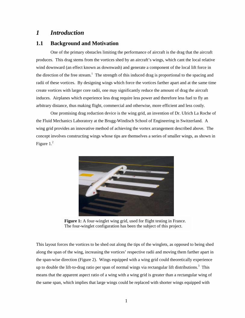
One promising drag reduction device is the wing grid, an invention of Dr. Ulrich La Roche of

the Fluid Mechanics Laboratory at the Brugg-Windisch School of Engineering in Switzerland. A

wing grid provides an innovative method of achieving the vortex arrangement described above. The

concept involves constructing wings whose tips are themselves a series of smaller wings, as shown in

Figure 1.2

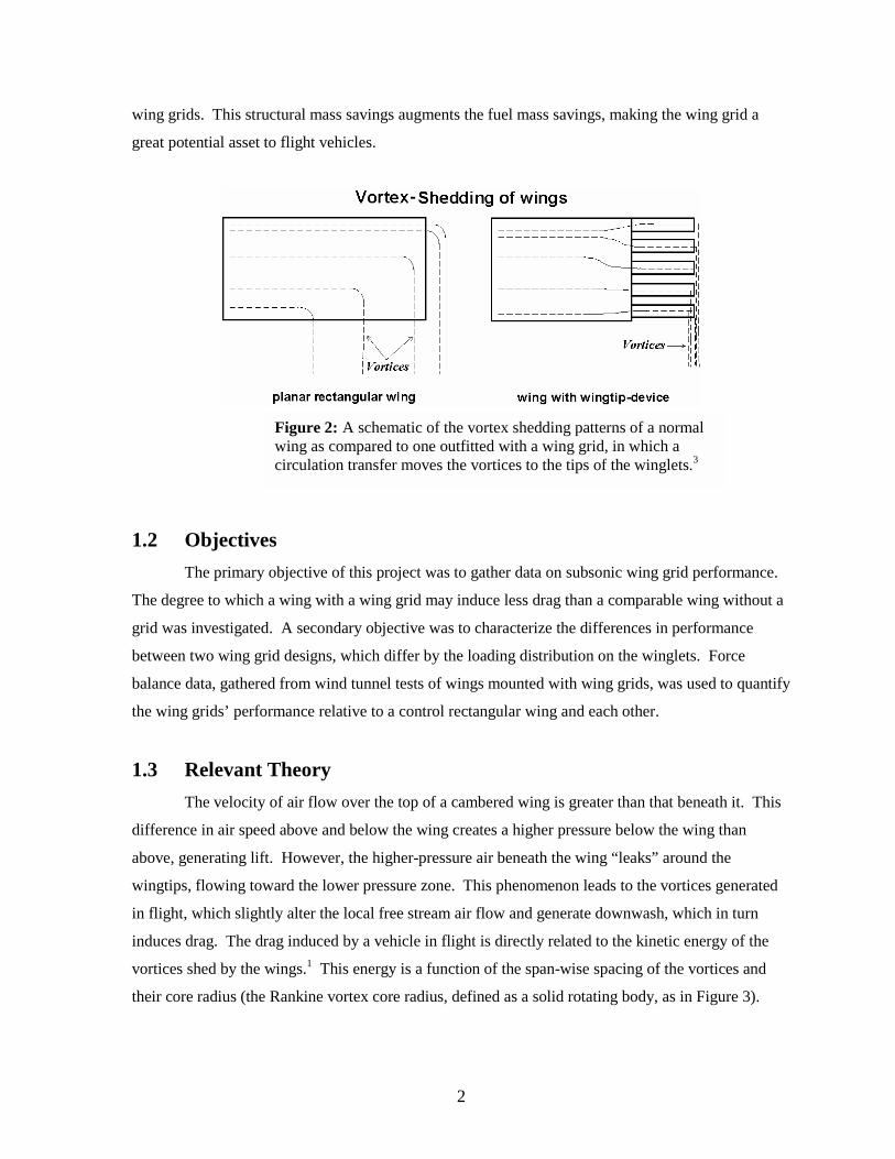
This layout forces the vortices to be shed out along the tips of the winglets, as opposed to being shed

along the span of the wing, increasing the vortices’ respective radii and moving them farther apart in

the span-wise direction (Figure 2). Wings equipped with a wing grid could theoretically experience

up to double the lift-to-drag ratio per span of normal wings via rectangular lift distributions.3 This

means that the apparent aspect ratio of a wing with a wing grid is greater than a rectangular wing of

the same span, which implies that large wings could be replaced with shorter wings equipped with

Figure 1: A four-winglet wing grid, used for flight testing in France. The four-winglet configuration has been the subject of this project.

2

wing grids. This structural mass savings augments the fuel mass savings, making the wing grid a

great potential asset to flight vehicles.

1.2 Objectives The primary objective of this project was to gather data on subsonic wing grid performance.

The degree to which a wing with a wing grid may induce less drag than a comparable wing without a

grid was investigated. A secondary objective was to characterize the differences in performance

between two wing grid designs, which differ by the loading distribution on the winglets. Force

balance data, gathered from wind tunnel tests of wings mounted with wing grids, was used to quantify

the wing grids’ performance relative to a control rectangular wing and each other.

1.3 Relevant Theory The velocity of air flow over the top of a cambered wing is greater than that beneath it. This

difference in air speed above and below the wing creates a higher pressure below the wing than

above, generating lift. However, the higher-pressure air beneath the wing “leaks” around the

wingtips, flowing toward the lower pressure zone. This phenomenon leads to the vortices generated

in flight, which slightly alter the local free stream air flow and generate downwash, which in turn

induces drag. The drag induced by a vehicle in flight is directly related to the kinetic energy of the

vortices shed by the wings.1 This energy is a function of the span-wise spacing of the vortices and

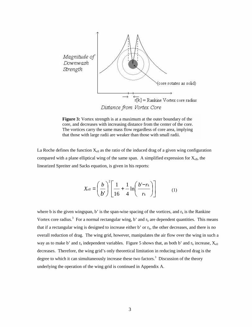
their core radius (the Rankine vortex core radius, defined as a solid rotating body, as in Figure 3).

Figure 2: A schematic of the vortex shedding patterns of a normal wing as compared to one outfitted with a wing grid, in which a circulation transfer moves the vortices to the tips of the winglets.3

3

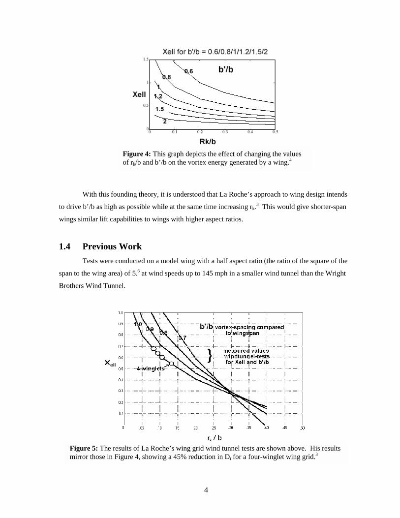
La Roche defines the function Xell as the ratio of the induced drag of a given wing configuration

compared with a plane elliptical wing of the same span. A simplified expression for Xell, the

linearized Spreiter and Sacks equation, is given in his reports:

−+=

k

kell

rrbb

Xb

'ln

41

161

2

' (1)

where b is the given wingspan, b’ is the span-wise spacing of the vortices, and rk is the Rankine

Vortex core radius.3 For a normal rectangular wing, b’ and rk are dependent quantities. This means

that if a rectangular wing is designed to increase either b’ or rk, the other decreases, and there is no

overall reduction of drag. The wing grid, however, manipulates the air flow over the wing in such a

way as to make b’ and rk independent variables. Figure 5 shows that, as both b’ and rk increase, Xell

decreases. Therefore, the wing grid’s only theoretical limitation in reducing induced drag is the

degree to which it can simultaneously increase these two factors.3 Discussion of the theory

underlying the operation of the wing grid is continued in Appendix A.

Figure 3: Vortex strength is at a maximum at the outer boundary of the core, and decreases with increasing distance from the center of the core. The vortices carry the same mass flow regardless of core area, implying that those with large radii are weaker than those with small radii.

4

With this founding theory, it is understood that La Roche’s approach to wing design intends

to drive b’/b as high as possible while at the same time increasing rk.3 This would give shorter-span

wings similar lift capabilities to wings with higher aspect ratios.

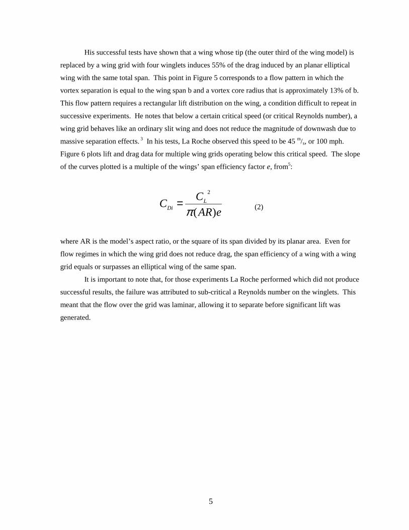
1.4 Previous Work Tests were conducted on a model wing with a half aspect ratio (the ratio of the square of the

span to the wing area) of 5.6 at wind speeds up to 145 mph in a smaller wind tunnel than the Wright

Brothers Wind Tunnel.

Figure 4: This graph depicts the effect of changing the values of rk/b and b’/b on the vortex energy generated by a wing.4

Figure 5: The results of La Roche’s wing grid wind tunnel tests are shown above. His results mirror those in Figure 4, showing a 45% reduction in Di for a four-winglet wing grid.3

5

His successful tests have shown that a wing whose tip (the outer third of the wing model) is

replaced by a wing grid with four winglets induces 55% of the drag induced by an planar elliptical

wing with the same total span. This point in Figure 5 corresponds to a flow pattern in which the

vortex separation is equal to the wing span b and a vortex core radius that is approximately 13% of b.

This flow pattern requires a rectangular lift distribution on the wing, a condition difficult to repeat in

successive experiments. He notes that below a certain critical speed (or critical Reynolds number), a

wing grid behaves like an ordinary slit wing and does not reduce the magnitude of downwash due to

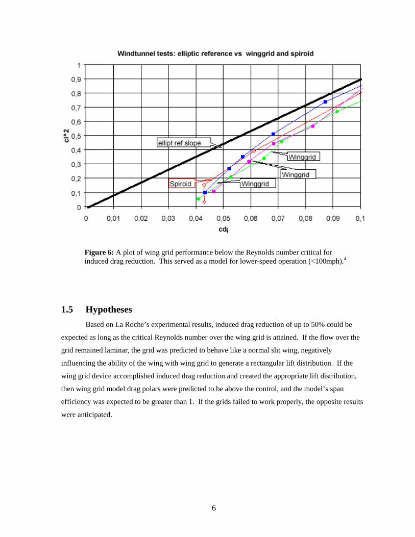
massive separation effects. 3 In his tests, La Roche observed this speed to be 45 m/s, or 100 mph.

Figure 6 plots lift and drag data for multiple wing grids operating below this critical speed. The slope

of the curves plotted is a multiple of the wings’ span efficiency factor e, from5:

eARCC L

Di )(

2

π= (2)

where AR is the model’s aspect ratio, or the square of its span divided by its planar area. Even for

flow regimes in which the wing grid does not reduce drag, the span efficiency of a wing with a wing

grid equals or surpasses an elliptical wing of the same span.

It is important to note that, for those experiments La Roche performed which did not produce

successful results, the failure was attributed to sub-critical a Reynolds number on the winglets. This

meant that the flow over the grid was laminar, allowing it to separate before significant lift was

generated.

6

1.5 Hypotheses

Based on La Roche’s experimental results, induced drag reduction of up to 50% could be

expected as long as the critical Reynolds number over the wing grid is attained. If the flow over the

grid remained laminar, the grid was predicted to behave like a normal slit wing, negatively

influencing the ability of the wing with wing grid to generate a rectangular lift distribution. If the

wing grid device accomplished induced drag reduction and created the appropriate lift distribution,

then wing grid model drag polars were predicted to be above the control, and the model’s span

efficiency was expected to be greater than 1. If the grids failed to work properly, the opposite results

were anticipated.

Figure 6: A plot of wing grid performance below the Reynolds number critical for induced drag reduction. This served as a model for lower-speed operation (<100mph).4

7

2 Technical Approach To quantify the extent to which a wing grid reduces the induced drag a wing generates, three

wing configurations, each consisting of a main wing body and one of three modular wing tips, were

tested in the MIT Wright Brothers Wind Tunnel (WBWT). The wing tips consisted of two different

wing grid designs and a control wing tip with the same chord and airfoil type as the main wing.

Details of model construction are treated in this section. The completed models were mounted on the

six-component pyramidal force balance in the WBWT and moved through a range of angles of attack

at three wind speeds. Drag polars were formed from the force data registered on the model at each

speed, and plots of CL2 vs. CDi were made to compare with La Roche’s previous results.

2.1 Model Construction 2.1.1 Wing Grid Design

Two four-winglet wing grids were constructed for this project, one in which all the winglets

are at approximately the same angle of attack (AOA) relative to the main wing section, and another in

which each winglet experiences roughly the same aerodynamic loading. La Roche provided the

empirical methodology to follow in designing the wing grids’ geometries. Table 1 summarizes the

critical dimensions of each grid.

Grid Type Winglet Chord Stagger Angle Winglet Spacing Winglet Rotation Angles

Equal-AOA 3.1 inches 8.3º 5.2 inches 0º, 0º, 0º, 0º

Equal-Load 3.1 inches 20º 5.1 inches -13.4º, -8.1º, -4.1º, 1.3º

The stagger angle is defined as the angle between the line of winglets and the chord line of the main

wing. Winglet spacing refers to the distance between adjacent winglets’ leading edges, and their

rotation angles are referenced from the main wing’s 0º AOA orientation (listed from leading to

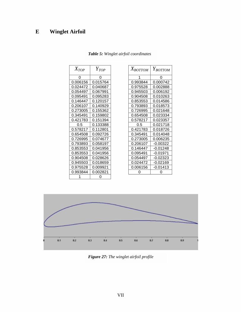
trailing winglet). The coordinates defining the winglet airfoil section were also provided by La

Roche (see Appendix E). The main wing airfoil was chosen to be the SD7037 because a cusp trailing

edge, good low AOA flight characteristics, and a high stall AOA were desirable. The last was

important because the wing grids’ performance over a large range of AOA was to be investigated.

Table 1: Defining quantities of wing grid geometry.

8

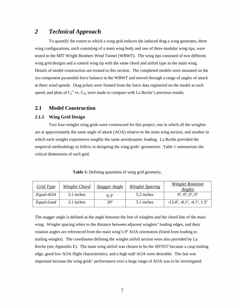
2.1.2 Superstructure and Wing Sections The main function of the model’s superstructure was to provide the main wing and winglets

with appropriate bending stiffness while still being feasible to construct. Thus the main wing section

was comprised of two steel spars, one at the quarter-chord and the other at the three-quarter-chord,

welded between two steel endplates, as shown in Figure 7.

The forward spar was thicker, to provide the majority of the required stiffness, while the aft

spar served to augment the first and prevent the wing from pitching. The endplates provided a means

of attaching the main wing to each of the wing tips and the force balance. The control tip structure

was similarly manufactured, as were the wing grids. Each winglet was held in place by fore and aft

spars welded between two endplates. The wing and winglets were cut from polystyrene foam using a

computer-numerical-controlled hot wire cutter and epoxied to their respective spars. Finally, the

wing and winglets were covered in two layers of fiberglass laminate and sanded smooth. The

completed models are shown in Figure 8.

Figure 7: The completed superstructure of the main wing and the Equal-Load wing grid.

Figure 8: From left to right, the finished Equal-Load and Equal-AOA wing grids, and the control tip.

9

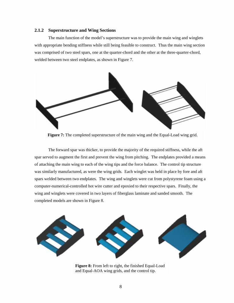
A special piece also had to be created to mate the main wing root endplate to the force

balance, which is sunk beneath the tunnel floor. This piece, the force balance interface, is shown in

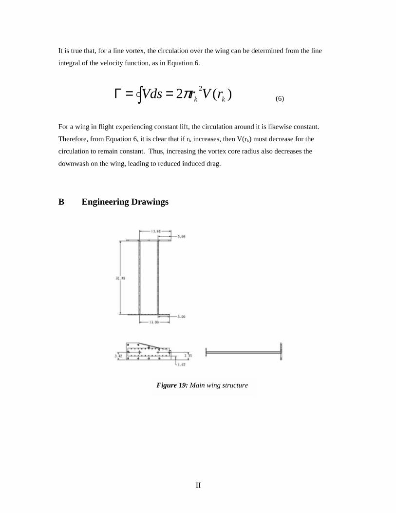
Figure 9. Appendix B contains engineering drawings for all parts of the model.

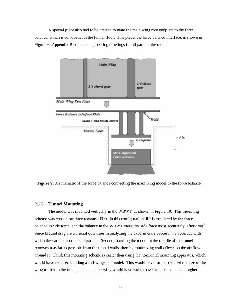
2.1.3 Tunnel Mounting The model was mounted vertically in the WBWT, as shown in Figure 10. This mounting

scheme was chosen for three reasons. First, in this configuration, lift is measured by the force

balance as side force, and the balance in the WBWT measures side force most accurately, after drag.6

Since lift and drag are a crucial quantities in analyzing the experiment’s success, the accuracy with

which they are measured is important. Second, standing the model in the middle of the tunnel

removes it as far as possible from the tunnel walls, thereby minimizing wall effects on the air flow

around it. Third, this mounting scheme is easier than using the horizontal mounting apparatus, which

would have required building a full-wingspan model. This would have further reduced the size of the

wing to fit it in the tunnel, and a smaller wing would have had to have been tested at even higher

Figure 9: A schematic of the force balance connecting the main wing model to the force balance.

10

velocities to achieve the flow regime (the Reynolds number over the wing grid) in which the wing

grid affects the induced drag.

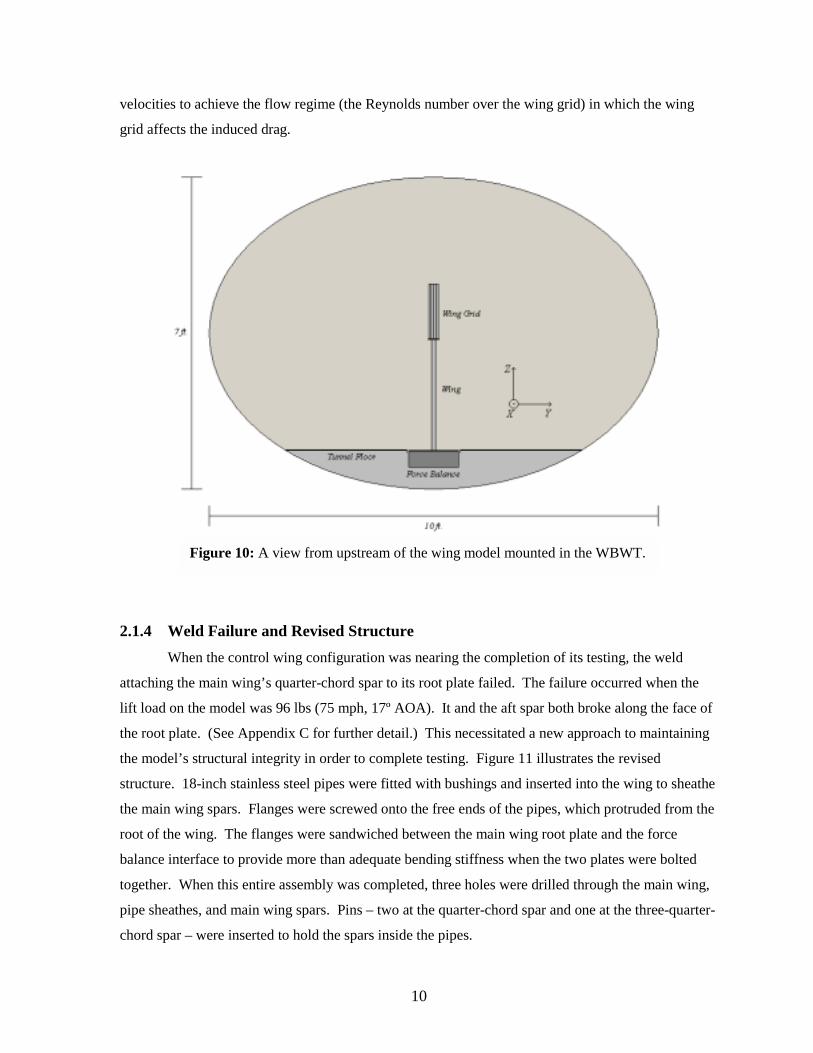
2.1.4 Weld Failure and Revised Structure When the control wing configuration was nearing the completion of its testing, the weld

attaching the main wing’s quarter-chord spar to its root plate failed. The failure occurred when the

lift load on the model was 96 lbs (75 mph, 17º AOA). It and the aft spar both broke along the face of

the root plate. (See Appendix C for further detail.) This necessitated a new approach to maintaining

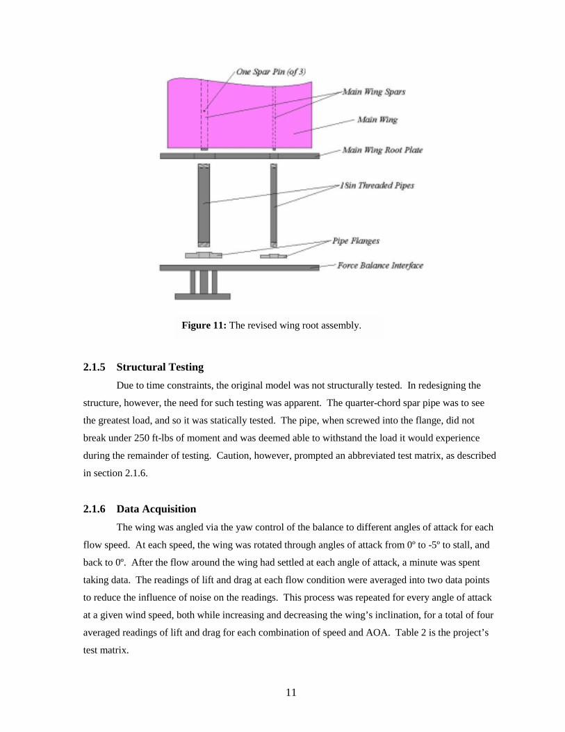
the model’s structural integrity in order to complete testing. Figure 11 illustrates the revised

structure. 18-inch stainless steel pipes were fitted with bushings and inserted into the wing to sheathe

the main wing spars. Flanges were screwed onto the free ends of the pipes, which protruded from the

root of the wing. The flanges were sandwiched between the main wing root plate and the force

balance interface to provide more than adequate bending stiffness when the two plates were bolted

together. When this entire assembly was completed, three holes were drilled through the main wing,

pipe sheathes, and main wing spars. Pins – two at the quarter-chord spar and one at the three-quarter-

chord spar – were inserted to hold the spars inside the pipes.

Figure 10: A view from upstream of the wing model mounted in the WBWT.

11

2.1.5 Structural Testing Due to time constraints, the original model was not structurally tested. In redesigning the

structure, however, the need for such testing was apparent. The quarter-chord spar pipe was to see

the greatest load, and so it was statically tested. The pipe, when screwed into the flange, did not

break under 250 ft-lbs of moment and was deemed able to withstand the load it would experience

during the remainder of testing. Caution, however, prompted an abbreviated test matrix, as described

in section 2.1.6.

2.1.6 Data Acquisition

The wing was angled via the yaw control of the balance to different angles of attack for each

flow speed. At each speed, the wing was rotated through angles of attack from 0º to -5º to stall, and

back to 0º. After the flow around the wing had settled at each angle of attack, a minute was spent

taking data. The readings of lift and drag at each flow condition were averaged into two data points

to reduce the influence of noise on the readings. This process was repeated for every angle of attack

at a given wind speed, both while increasing and decreasing the wing’s inclination, for a total of four

averaged readings of lift and drag for each combination of speed and AOA. Table 2 is the project’s

test matrix.

Figure 11: The revised wing root assembly.

12

-5 -4 … 10 11 … 18

( ° α )

30 (mph) 4 4 … 4 4 … 4

45 4 4 … 4 4 … 4

60 4 4 … 4 0 … 0

The original test matrix called for running the tunnel at 5 mph increments between 30 mph

and 100 mph, in the interests of clearly resolving the speed range over which the wing grid effect

occurs. The abbreviated range of flow speeds at which data was taken was a result of the weld

failure. As an additional precautionary measure, the safety margin for aerodynamic loading on the

model was increased, which accounts for the fact that no data was taken at high AOA at 60 mph. The

data output by the wind tunnel data collection software yielded the magnitude of the force

components on the wing and a value of dynamic head corrected for humidity, which allowed the lift

and drag coefficients to be calculated directly. These coefficients drive the analysis quantifying the

wing grids’ ability to reduce induced drag.

3 Results 3.1 Data Processing

For each wing configuration at each speed, the drag at zero-lift was determined as well as the

data allowed and was subtracted from the measured values of drag to find CDi. From CL and CDi, drag

polars for all the data sets were produced. Polars from the 30 mph data have been omitted because

the data was extremely scattered, especially at low AOA, and it was very difficult to establish trends

from the plots. Moreover, excluding these data is further justified by the trend visible in the 45 and

60 mph data. The wing grids’ performance improved as wind speed increased, so neglecting this data

only removes the worst case from consideration.

Table 2: The testing matrix for each of the three wing configurations, showing that four readings were taken at each flow condition.

13

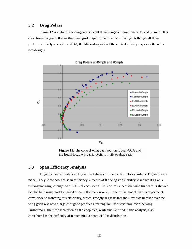
3.2 Drag Polars Figure 12 is a plot of the drag polars for all three wing configurations at 45 and 60 mph. It is

clear from this graph that neither wing grid outperformed the control wing. Although all three

perform similarly at very low AOA, the lift-to-drag ratio of the control quickly surpasses the other

two designs.

3.3 Span Efficiency Analysis To gain a deeper understanding of the behavior of the models, plots similar to Figure 6 were

made. They show how the span efficiency, a metric of the wing grids’ ability to reduce drag on a

rectangular wing, changes with AOA at each speed. La Roche’s successful wind tunnel tests showed

that his half-wing model attained a span efficiency near 2. None of the models in this experiment

came close to matching this efficiency, which strongly suggests that the Reynolds number over the

wing grids was never large enough to produce a rectangular lift distribution over the wing.

Furthermore, the flow separation on the endplates, while unquantified in this analysis, also

contributed to the difficulty of maintaining a beneficial lift distribution.

Figure 12: The control wing beat both the Equal-AOA and the Equal-Load wing grid designs in lift-to-drag ratio.

14

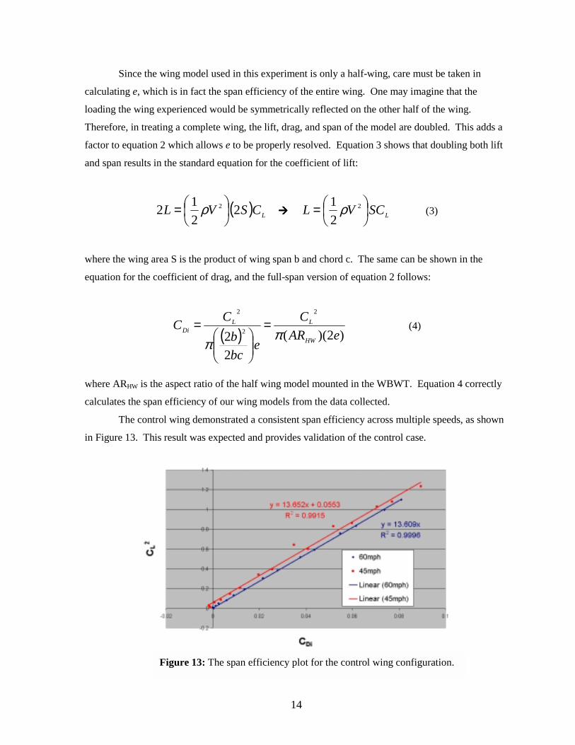
Since the wing model used in this experiment is only a half-wing, care must be taken in

calculating e, which is in fact the span efficiency of the entire wing. One may imagine that the

loading the wing experienced would be symmetrically reflected on the other half of the wing.

Therefore, in treating a complete wing, the lift, drag, and span of the model are doubled. This adds a

factor to equation 2 which allows e to be properly resolved. Equation 3 shows that doubling both lift

and span results in the standard equation for the coefficient of lift:

( ) LCSVL 2212 2

= ρ ���� LSCVL

= 2

21 ρ (3)

where the wing area S is the product of wing span b and chord c. The same can be shown in the

equation for the coefficient of drag, and the full-span version of equation 2 follows:

( ) )2)((22

2

2

2

eARC

ebcb

CCHW

LLDi π

π=

= (4)

where ARHW is the aspect ratio of the half wing model mounted in the WBWT. Equation 4 correctly

calculates the span efficiency of our wing models from the data collected.

The control wing demonstrated a consistent span efficiency across multiple speeds, as shown

in Figure 13. This result was expected and provides validation of the control case.

Figure 13: The span efficiency plot for the control wing configuration.

15

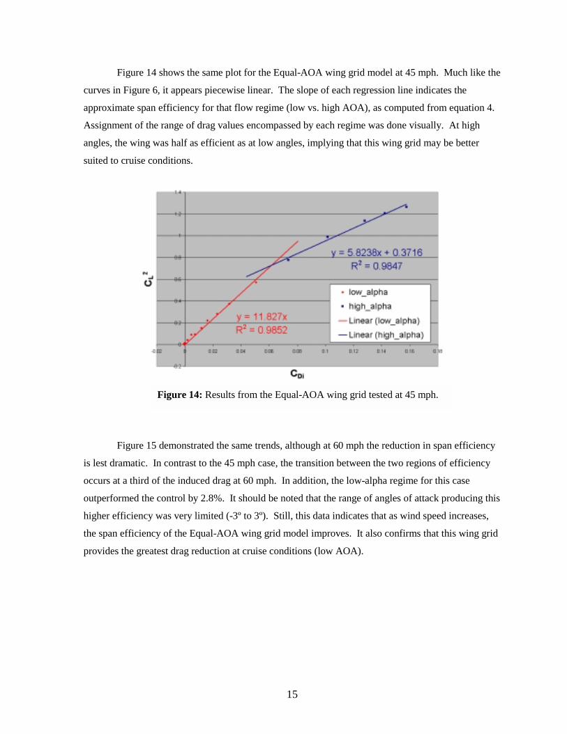
Figure 14 shows the same plot for the Equal-AOA wing grid model at 45 mph. Much like the

curves in Figure 6, it appears piecewise linear. The slope of each regression line indicates the

approximate span efficiency for that flow regime (low vs. high AOA), as computed from equation 4.

Assignment of the range of drag values encompassed by each regime was done visually. At high

angles, the wing was half as efficient as at low angles, implying that this wing grid may be better

suited to cruise conditions.

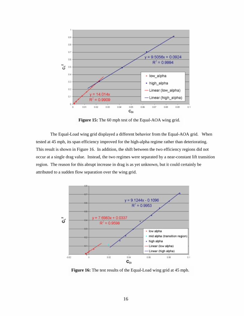
Figure 15 demonstrated the same trends, although at 60 mph the reduction in span efficiency

is lest dramatic. In contrast to the 45 mph case, the transition between the two regions of efficiency

occurs at a third of the induced drag at 60 mph. In addition, the low-alpha regime for this case

outperformed the control by 2.8%. It should be noted that the range of angles of attack producing this

higher efficiency was very limited (-3º to 3º). Still, this data indicates that as wind speed increases,

the span efficiency of the Equal-AOA wing grid model improves. It also confirms that this wing grid

provides the greatest drag reduction at cruise conditions (low AOA).

Figure 14: Results from the Equal-AOA wing grid tested at 45 mph.

16

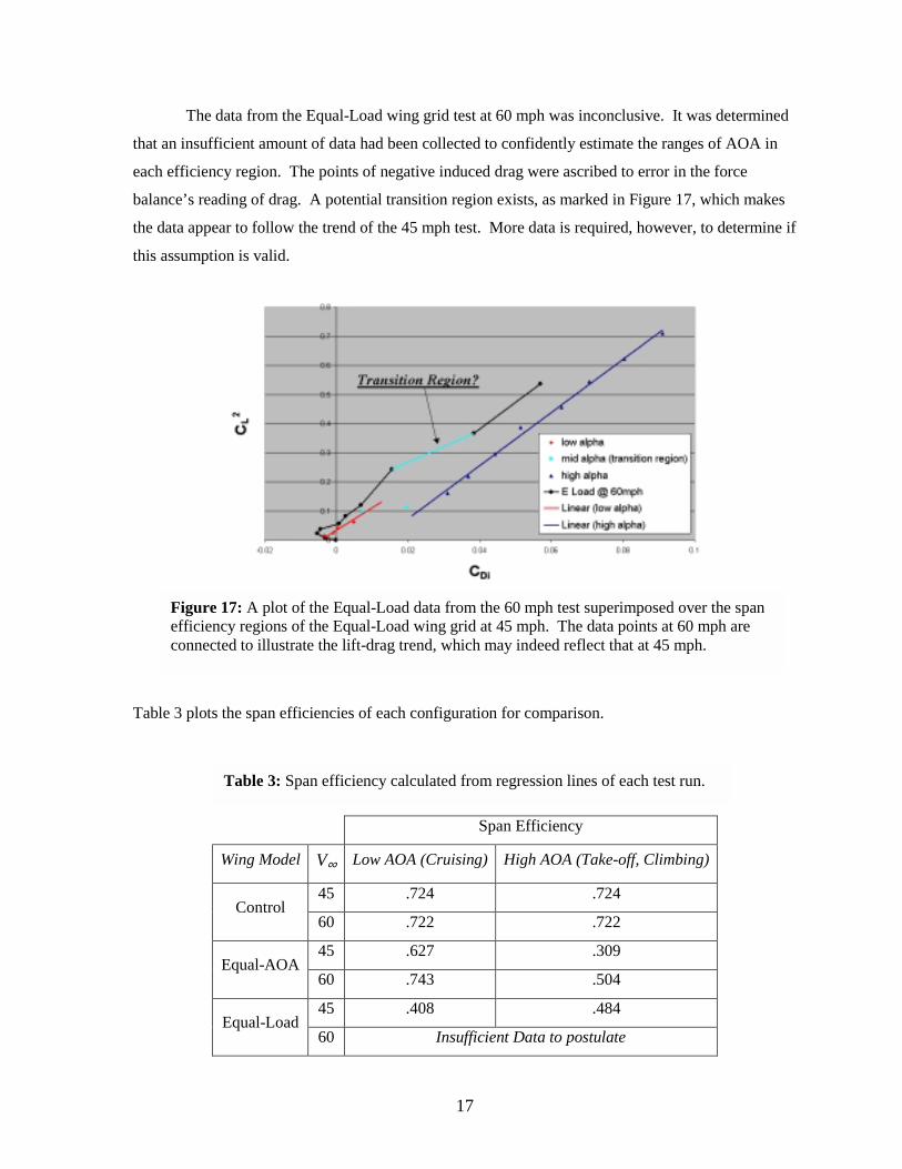
The Equal-Load wing grid displayed a different behavior from the Equal-AOA grid. When

tested at 45 mph, its span efficiency improved for the high-alpha regime rather than deteriorating.

This result is shown in Figure 16. In addition, the shift between the two efficiency regions did not

occur at a single drag value. Instead, the two regimes were separated by a near-constant lift transition

region. The reason for this abrupt increase in drag is as yet unknown, but it could certainly be

attributed to a sudden flow separation over the wing grid.

Figure 15: The 60 mph test of the Equal-AOA wing grid.

Figure 16: The test results of the Equal-Load wing grid at 45 mph.

17

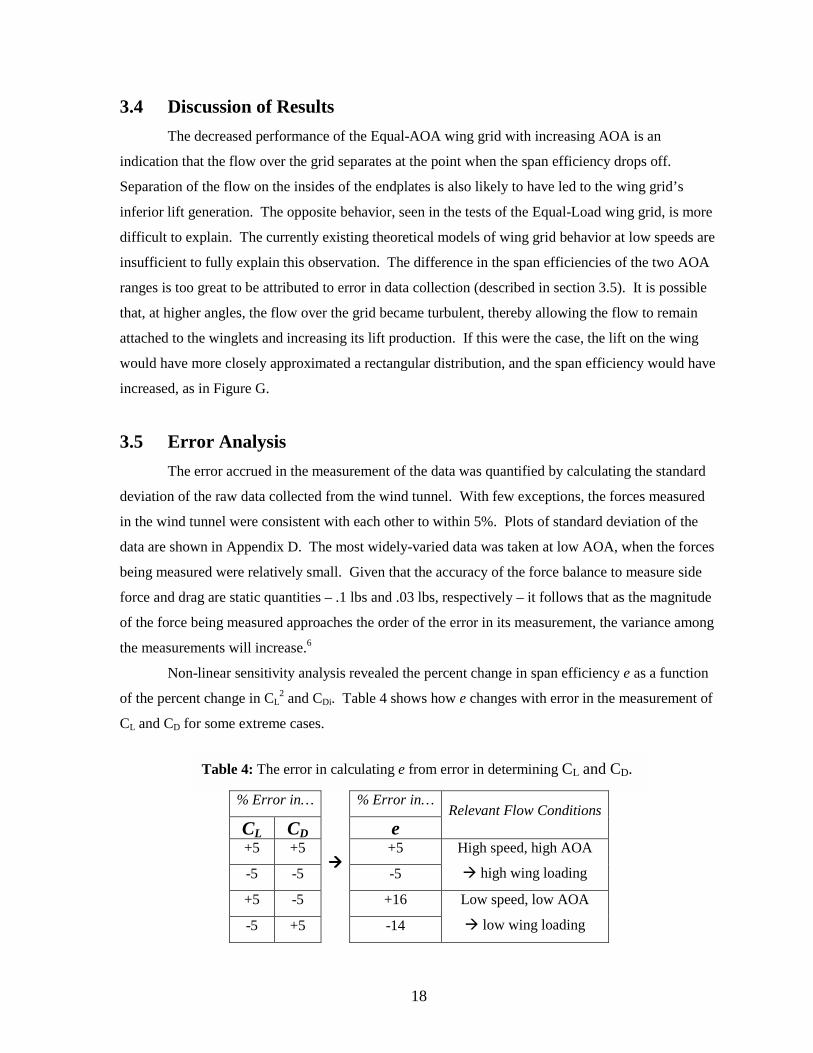
The data from the Equal-Load wing grid test at 60 mph was inconclusive. It was determined

that an insufficient amount of data had been collected to confidently estimate the ranges of AOA in

each efficiency region. The points of negative induced drag were ascribed to error in the force

balance’s reading of drag. A potential transition region exists, as marked in Figure 17, which makes

the data appear to follow the trend of the 45 mph test. More data is required, however, to determine if

this assumption is valid.

Table 3 plots the span efficiencies of each configuration for comparison.

Span Efficiency

Wing Model V∞ Low AOA (Cruising) High AOA (Take-off, Climbing)

45 .724 .724 Control

60 .722 .722

45 .627 .309 Equal-AOA

60 .743 .504

45 .408 .484 Equal-Load

60 Insufficient Data to postulate

Figure 17: A plot of the Equal-Load data from the 60 mph test superimposed over the span efficiency regions of the Equal-Load wing grid at 45 mph. The data points at 60 mph are connected to illustrate the lift-drag trend, which may indeed reflect that at 45 mph.

Table 3: Span efficiency calculated from regression lines of each test run.

18

3.4 Discussion of Results The decreased performance of the Equal-AOA wing grid with increasing AOA is an

indication that the flow over the grid separates at the point when the span efficiency drops off.

Separation of the flow on the insides of the endplates is also likely to have led to the wing grid’s

inferior lift generation. The opposite behavior, seen in the tests of the Equal-Load wing grid, is more

difficult to explain. The currently existing theoretical models of wing grid behavior at low speeds are

insufficient to fully explain this observation. The difference in the span efficiencies of the two AOA

ranges is too great to be attributed to error in data collection (described in section 3.5). It is possible

that, at higher angles, the flow over the grid became turbulent, thereby allowing the flow to remain

attached to the winglets and increasing its lift production. If this were the case, the lift on the wing

would have more closely approximated a rectangular distribution, and the span efficiency would have

increased, as in Figure G.

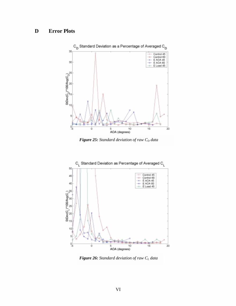
3.5 Error Analysis The error accrued in the measurement of the data was quantified by calculating the standard

deviation of the raw data collected from the wind tunnel. With few exceptions, the forces measured

in the wind tunnel were consistent with each other to within 5%. Plots of standard deviation of the

data are shown in Appendix D. The most widely-varied data was taken at low AOA, when the forces

being measured were relatively small. Given that the accuracy of the force balance to measure side

force and drag are static quantities – .1 lbs and .03 lbs, respectively – it follows that as the magnitude

of the force being measured approaches the order of the error in its measurement, the variance among

the measurements will increase.6

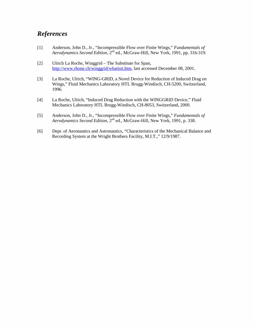
Non-linear sensitivity analysis revealed the percent change in span efficiency e as a function

of the percent change in CL2 and CDi. Table 4 shows how e changes with error in the measurement of

CL and CD for some extreme cases.

% Error in… % Error in…

CL CD e Relevant Flow Conditions

+5 +5 +5

-5 -5 -5

High speed, high AOA

� high wing loading

+5 -5 +16

-5 +5

����

-14

Low speed, low AOA

� low wing loading

Table 4: The error in calculating e from error in determining CL and CD.

19

When the percent error in CL and CD are of opposite signs, the model experienced wobble as it was

buffeted by the wind. The wing grids created wakes and eddies that caused the wing to move slightly

from side to side. Under these conditions, the accuracy with which span efficiency can be determined

decreases significantly, as shown in Appendix D.

4 Conclusions It is clear from the data gathered that the wing grid has a negative effect on flight

performance at low speeds. The flow over it tends to separate before the wing generates a rectangular

lift distribution. The critical flow regime, in which the Reynolds number over the grid is sufficiently

large and the wing grid effect reduces induced drag, was not reached. The data does, however, imply

that at higher speeds, the wing grid effect may be present at low (cruising) angles of attack, as La

Roche predicts.

4.1 Future Work The wing grid is a promising design, and the results obtained in this study demand further

work be done to characterize the device’s performance over a larger set of flow regimes. All three

models – both wing grid configurations and the control – should be tested at speeds at and above 100

mph, so that the critical Reynolds number can be attained. In addition, a functional relationship

between span efficiency and flow regime should be determined, or, in lieu of this, a quantified

heuristic model. Finally, efforts should be made to connect wing grid theory to a concrete

methodology for wing grid design. La Roche’s approach is no doubt sound, but still needs to be

elucidated for the benefit of the aeronautics community at large.

Acknowledgements The experimental project team would like to extend warm thanks to the following

individuals: Don Weiner for his machine shop expertise and all of his time, Dick Perdichizzi for his

invaluable assistance in the wind tunnel, Professor Eugene Covert for his guidance over the past year,

and Dr. Ulrich La Roche for his continued correspondence that helped build a better wing grid.

References

[1] Anderson, John D., Jr., “Incompressible Flow over Finite Wings,” Fundamentals of Aerodynamics Second Edition, 2nd ed., McGraw-Hill, New York, 1991, pp. 316-319.

[2] Ulrich La Roche, Winggrid – The Substitute for Span,

http://www.rhone.ch/winggrid/whatisit.htm, last accessed December 08, 2001. [3] La Roche, Ulrich, “WING-GRID, a Novel Device for Reduction of Induced Drag on

Wings,” Fluid Mechanics Laboratory HTL Brugg-Windisch, CH-5200, Switzerland, 1996.

[4] La Roche, Ulrich, “Induced Drag Reduction with the WINGGRID Device,” Fluid

Mechanics Laboratory HTL Brugg-Windisch, CH-8053, Switzerland, 2000. [5] Anderson, John D., Jr., “Incompressible Flow over Finite Wings,” Fundamentals of

Aerodynamics Second Edition, 2nd ed., McGraw-Hill, New York, 1991, p. 338. [6] Dept. of Aeronautics and Astronautics, “Characteristics of the Mechanical Balance and

Recording System at the Wright Brothers Facility, M.I.T.,” 12/9/1987.

I

Appendices

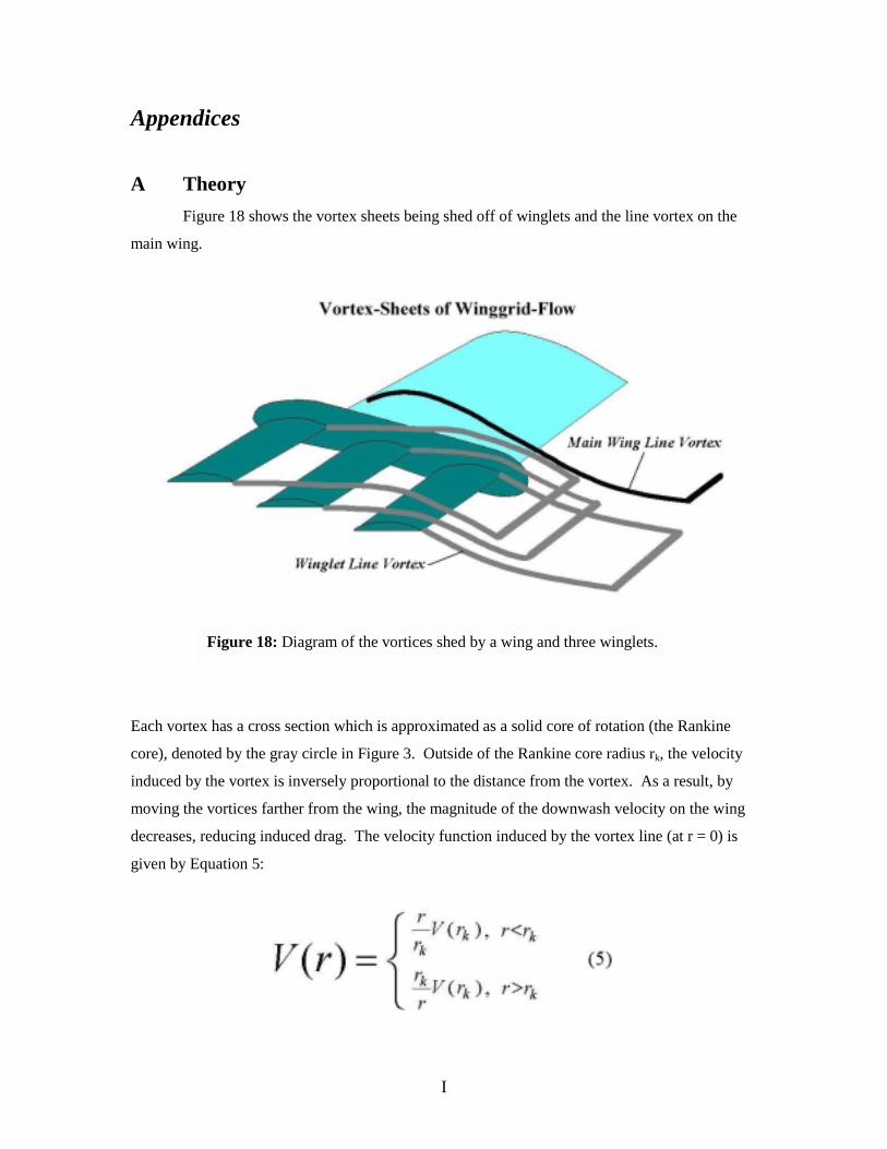
A Theory Figure 18 shows the vortex sheets being shed off of winglets and the line vortex on the

main wing.

Each vortex has a cross section which is approximated as a solid core of rotation (the Rankine

core), denoted by the gray circle in Figure 3. Outside of the Rankine core radius rk, the velocity

induced by the vortex is inversely proportional to the distance from the vortex. As a result, by

moving the vortices farther from the wing, the magnitude of the downwash velocity on the wing

decreases, reducing induced drag. The velocity function induced by the vortex line (at r = 0) is

given by Equation 5:

Figure 18: Diagram of the vortices shed by a wing and three winglets.

II

It is true that, for a line vortex, the circulation over the wing can be determined from the line

integral of the velocity function, as in Equation 6.

∫ ==Γ )(2 2kk rVrVds π (6)

For a wing in flight experiencing constant lift, the circulation around it is likewise constant.

Therefore, from Equation 6, it is clear that if rk increases, then V(rk) must decrease for the

circulation to remain constant. Thus, increasing the vortex core radius also decreases the

downwash on the wing, leading to reduced induced drag.

B Engineering Drawings

Figure 19: Main wing structure

III

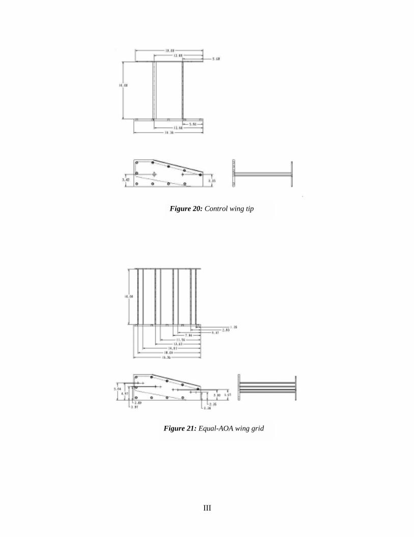
Figure 20: Control wing tip

Figure 21: Equal-AOA wing grid

IV

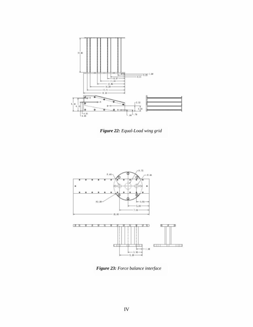
Figure 22: Equal-Load wing grid

Figure 23: Force balance interface

V

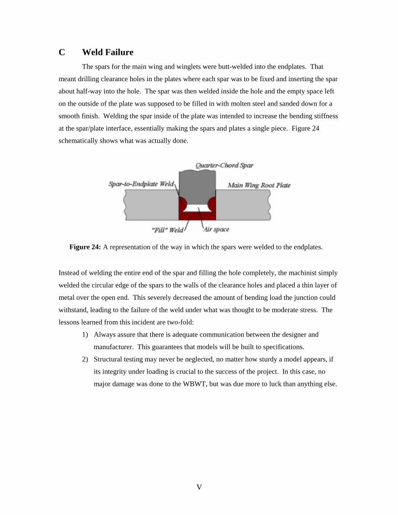
C Weld Failure The spars for the main wing and winglets were butt-welded into the endplates. That

meant drilling clearance holes in the plates where each spar was to be fixed and inserting the spar

about half-way into the hole. The spar was then welded inside the hole and the empty space left

on the outside of the plate was supposed to be filled in with molten steel and sanded down for a

smooth finish. Welding the spar inside of the plate was intended to increase the bending stiffness

at the spar/plate interface, essentially making the spars and plates a single piece. Figure 24

schematically shows what was actually done.

Instead of welding the entire end of the spar and filling the hole completely, the machinist simply

welded the circular edge of the spars to the walls of the clearance holes and placed a thin layer of

metal over the open end. This severely decreased the amount of bending load the junction could

withstand, leading to the failure of the weld under what was thought to be moderate stress. The

lessons learned from this incident are two-fold:

1) Always assure that there is adequate communication between the designer and

manufacturer. This guarantees that models will be built to specifications.

2) Structural testing may never be neglected, no matter how sturdy a model appears, if

its integrity under loading is crucial to the success of the project. In this case, no

major damage was done to the WBWT, but was due more to luck than anything else.

Figure 24: A representation of the way in which the spars were welded to the endplates.

VI

D Error Plots

Figure 25: Standard deviation of raw CD data

Figure 26: Standard deviation of raw CL data

VII

E Winglet Airfoil

XTOP YTOP XBOTTOM YBOTTOM

0 0 1 0 0.006156 0.015764 0.993844 0.000742 0.024472 0.040687 0.975528 0.002888 0.054497 0.067991 0.945503 0.006192 0.095491 0.095283 0.904508 0.010263 0.146447 0.120157 0.853553 0.014586 0.206107 0.140929 0.793893 0.018573 0.273005 0.155362 0.726995 0.021648 0.345491 0.159802 0.654508 0.023334 0.421783 0.151394 0.578217 0.023357

0.5 0.133388 0.5 0.021718 0.578217 0.112801 0.421783 0.018726 0.654508 0.092726 0.345491 0.014048 0.726995 0.074677 0.273005 0.006235 0.793893 0.058197 0.206107 -0.00322 0.853553 0.041956 0.146447 -0.01248 0.853553 0.041956 0.095491 -0.01971 0.904508 0.028626 0.054497 -0.02323 0.945503 0.018659 0.024472 -0.02169 0.975528 0.009921 0.006156 -0.01413 0.993844 0.002821 0 0

1 0

SPACE

Figure 27: The winglet airfoil profile

Table 5: Winglet airfoil coordinates