THE WKB APPROXIMATION FOR A

LINEAR POTENTIAL AND CEILING

A Thesis

by

TODD AUSTIN ZAPATA

Submitted to the Office of Graduate Studies ofTexas A&M University

in partial fulfillment of the requirements for the degree of

MASTER OF SCIENCE

December 2007

Major Subject: Physics

THE WKB APPROXIMATION FOR

A LINEAR POTENTIAL AND CEILING

A Thesis

by

TODD AUSTIN ZAPATA

Submitted to the Office of Graduate Studies ofTexas A&M University

in partial fulfillment of the requirements for the degree of

MASTER OF SCIENCE

Approved by:

Chair of Committee, Stephen A. FullingCommittee Members, Siu A. Chin

Guergana Petrova

Head of Department, Edward Fry

December 2007

Major Subject: Physics

iii

ABSTRACT

The WKB Approximation for a

Linear Potential and Ceiling. (December 2007)

Todd Austin Zapata, B.S., Texas A&M University

Chair of Advisory Committee: Dr. Stephen A Fulling

The physical problem this thesis deals with is a quantum system with linear

potential driving a particle away from a ceiling (impenetrable barrier). This thesis

will construct the WKB approximation of the quantum mechanical propagator. The

application of the approximation will be for propagators corresponding to both initial

momentum data and initial position data.

Although the analytic solution for the propagator exists, it is an indefinite inte-

gral of Airy functions and difficult to use in obtaining probability densities by numer-

ical integration or other schemes considered by the author. The WKB construction

is less problematic because it is representable in exact form, and integration schemes

(both numerical and analytic) to obtain probability densities are straightforward to

implement. Another purpose of this thesis is to be a starting point for the construc-

tion of WKB propagators with general potentials but the same type of boundary,

impenetrable barrier.

Research pertaining to this thesis includes determining all classical paths and

constraints for the one-dimensional linear potential with ceiling, and using these

equations to construct the classical action, and hence the WKB approximation. Also,

evaluation of final quantum wave functions using numerical integration to check and

better understand the approximation is part of the research.

The results indicate that the validity of the WKB approximation depends on the

type of classical paths (i.e. the initial data of the path) used in the construction.

iv

Specifically, the presence of the ceiling may cause the semi-classical wave packets

to become vanishingly small in one representation of initial classical data, while not

effecting the packets in another. The conclusion of this phenomenon is that the

representation where the packets are not annihilated is the correct representation.

v

To Mom and Dad, I love you very much.

vi

ACKNOWLEDGMENTS

I give all thanks and praise to Jesus Christ for the knowledge I have been blessed

with, and the men and women whom have guided me throughout this life.

Special thanks go to Dr. Stephen A. Fulling for taking me in as a beginner,

and never giving up on me, for listening to my crazy ideas with respect and having

confidence in my abilities, and for sharing his ingenious views of nature with me.

The funding for this project comes from the NSF grant PHYS-0554849.

vii

TABLE OF CONTENTS

CHAPTER Page

I INTRODUCTION . . . . . . . . . . . . . . . . . . . . . . . . . . 1

A. The Quantum and Classical System . . . . . . . . . . . . . 3

B. The Classical Solutions . . . . . . . . . . . . . . . . . . . . 6

C. The WKB Ansatz . . . . . . . . . . . . . . . . . . . . . . . 10

II TRAJECTORIES WITH GIVEN INITIAL POSITION DATA . 16

A. Trajectories of Type (1) . . . . . . . . . . . . . . . . . . . 18

B. Trajectories of Type (2) . . . . . . . . . . . . . . . . . . . 19

C. Trajectories of Type (3) . . . . . . . . . . . . . . . . . . . 20

D. Bounce Trajectories . . . . . . . . . . . . . . . . . . . . . . 22

E. The Classical Action . . . . . . . . . . . . . . . . . . . . . 28

F. The Amplitude . . . . . . . . . . . . . . . . . . . . . . . . 32

III TRAJECTORIES WITH GIVEN INITIAL MOMENTUM DATA 37

A. Trajectories of Type (1) . . . . . . . . . . . . . . . . . . . 39

B. Trajectories of Type (2) . . . . . . . . . . . . . . . . . . . 39

C. Trajectories of Type (3) . . . . . . . . . . . . . . . . . . . 40

D. Bounce Trajectories . . . . . . . . . . . . . . . . . . . . . . 41

E. The Classical Action . . . . . . . . . . . . . . . . . . . . . 46

F. The Amplitude . . . . . . . . . . . . . . . . . . . . . . . . 48

IV SUMMARY: COMPARISON OF THE WKB PROPAGATORS 51

A. The Initial Wave Packet . . . . . . . . . . . . . . . . . . . 51

B. The Propagators Constructed from Non-bounce Paths . . . 53

C. The Forbidden Region . . . . . . . . . . . . . . . . . . . . 55

REFERENCES . . . . . . . . . . . . . . . . . . . . . . . . . . . . . . . . . . . 59

VITA . . . . . . . . . . . . . . . . . . . . . . . . . . . . . . . . . . . . . . . . 60

viii

LIST OF TABLES

TABLE Page

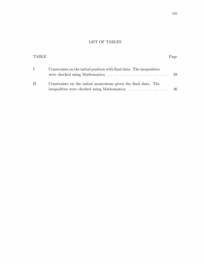
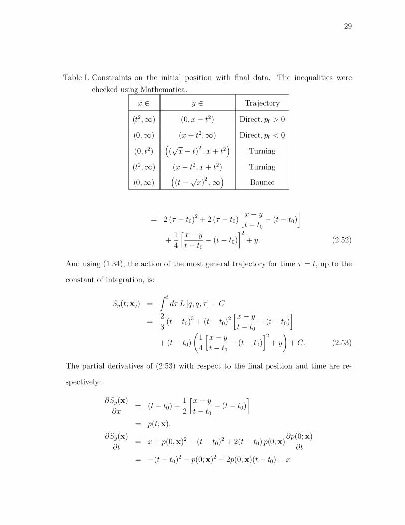
I Constraints on the initial position with final data. The inequalities

were checked using Mathematica. . . . . . . . . . . . . . . . . . . . . 29

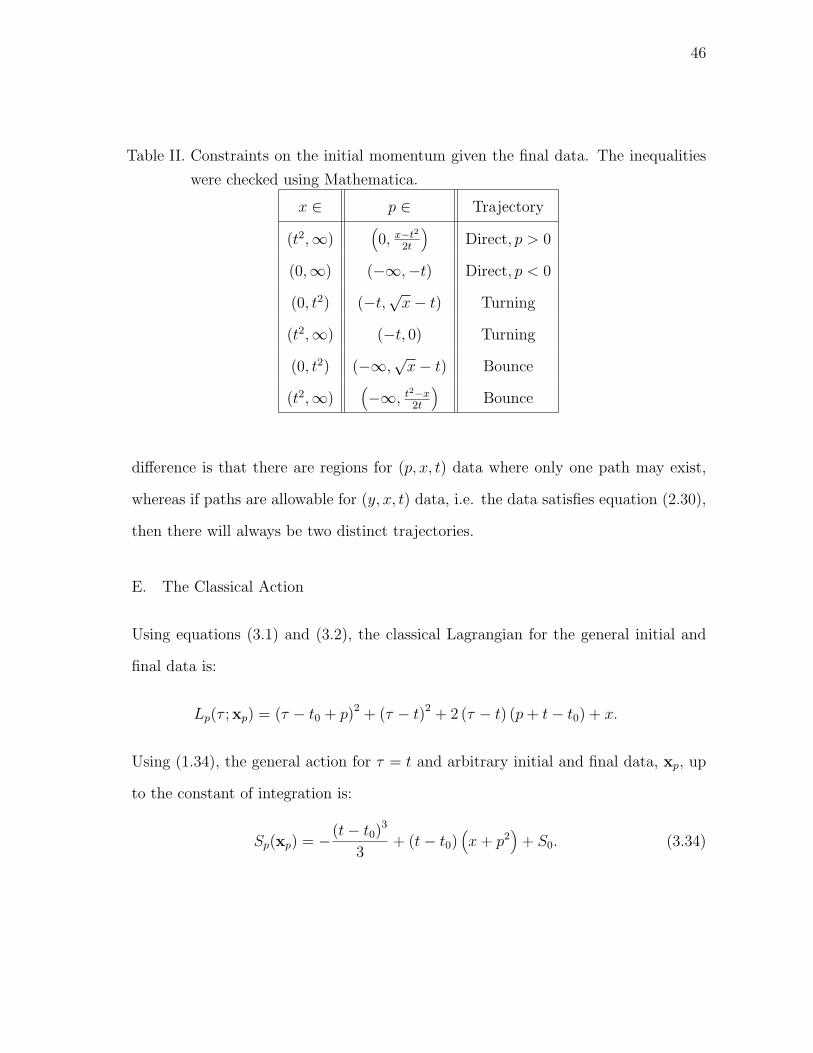
II Constraints on the initial momentum given the final data. The

inequalities were checked using Mathematica. . . . . . . . . . . . . . 46

ix

LIST OF FIGURES

FIGURE Page

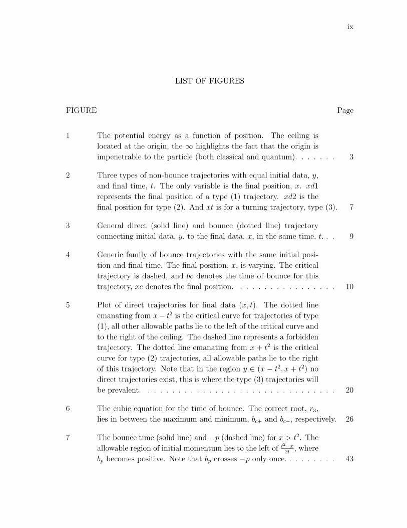
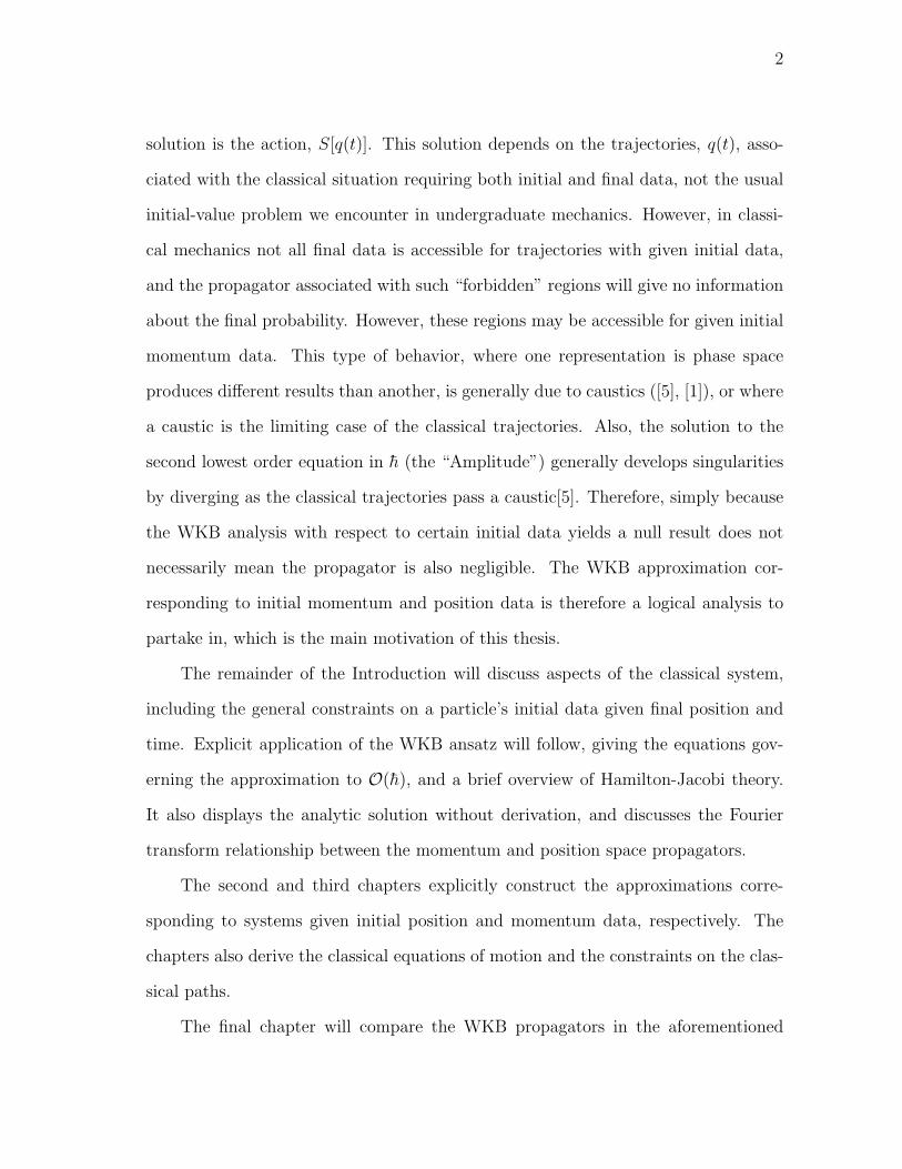
1 The potential energy as a function of position. The ceiling is

located at the origin, the ∞ highlights the fact that the origin is

impenetrable to the particle (both classical and quantum). . . . . . . 3

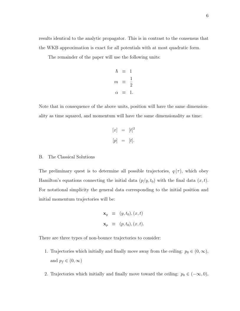
2 Three types of non-bounce trajectories with equal initial data, y,

and final time, t. The only variable is the final position, x. xd1

represents the final position of a type (1) trajectory. xd2 is the

final position for type (2). And xt is for a turning trajectory, type (3). 7

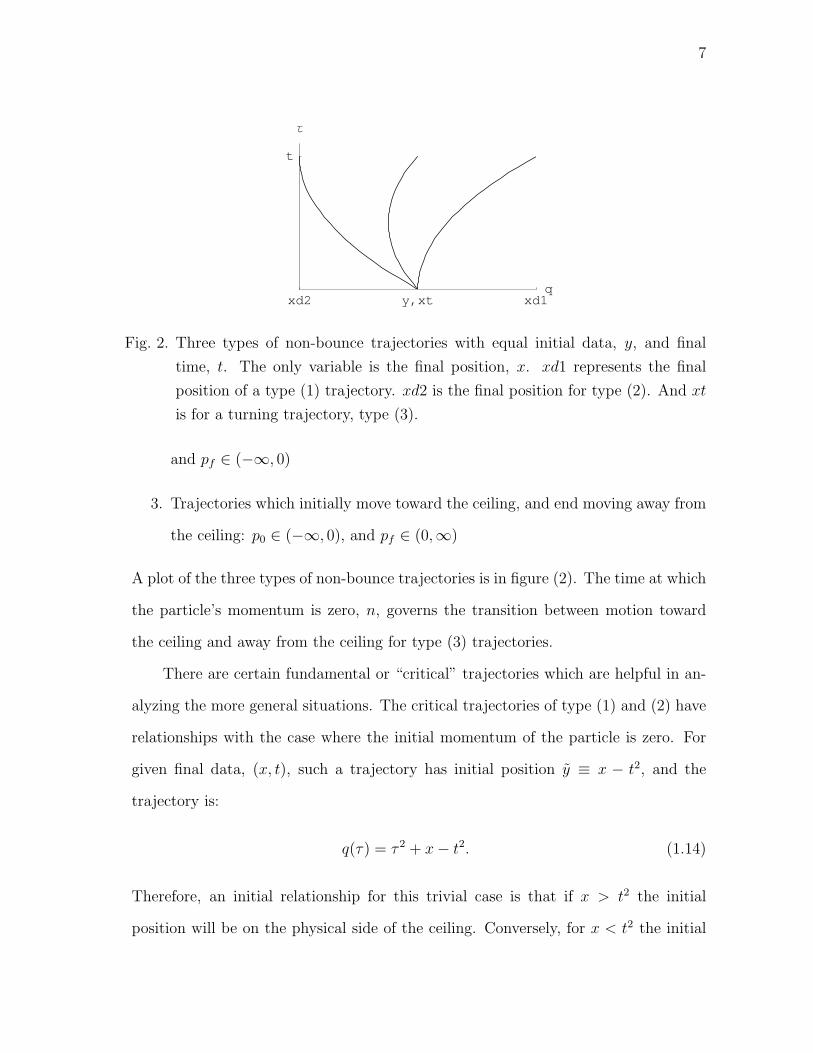
3 General direct (solid line) and bounce (dotted line) trajectory

connecting initial data, y, to the final data, x, in the same time, t. . . 9

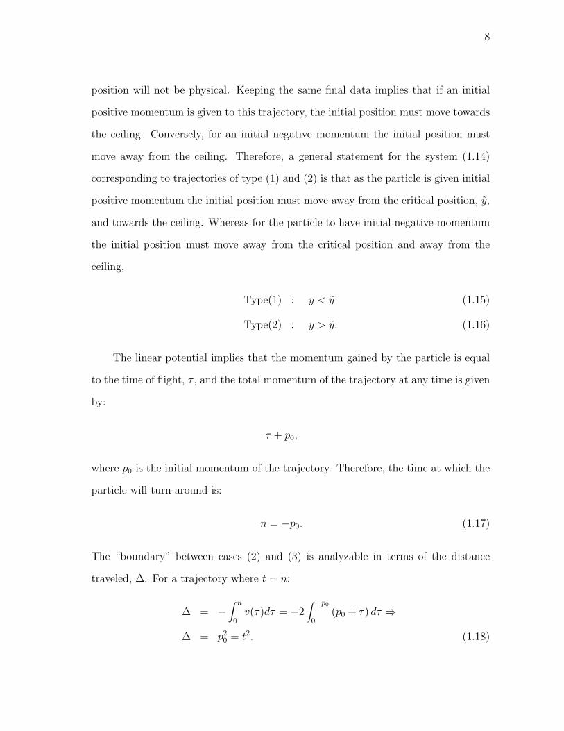
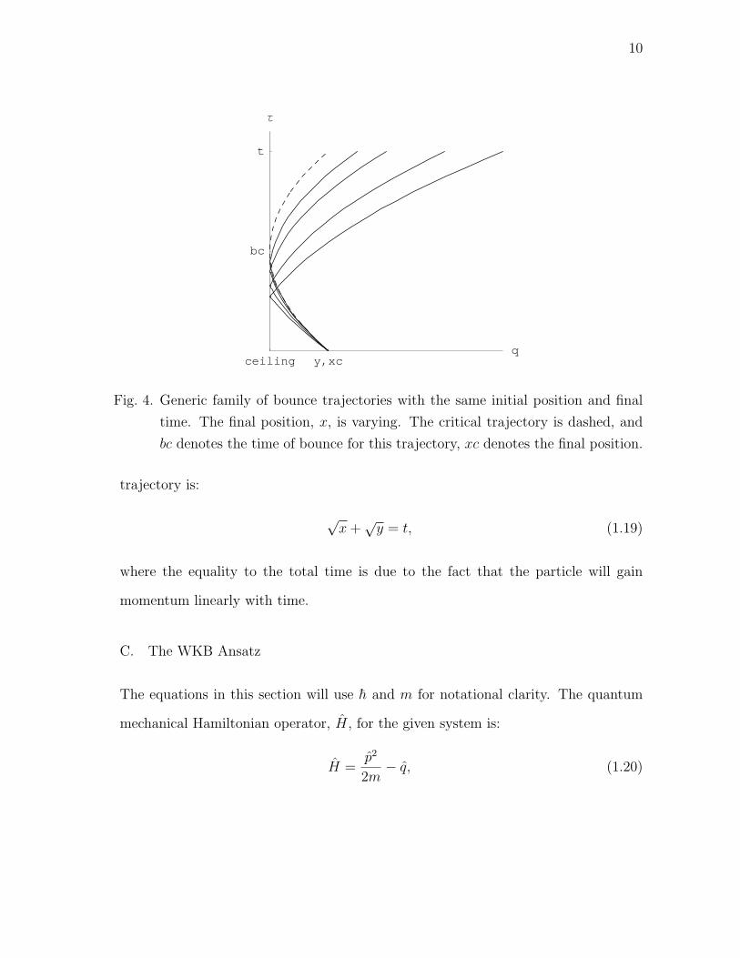
4 Generic family of bounce trajectories with the same initial posi-

tion and final time. The final position, x, is varying. The critical

trajectory is dashed, and bc denotes the time of bounce for this

trajectory, xc denotes the final position. . . . . . . . . . . . . . . . . 10

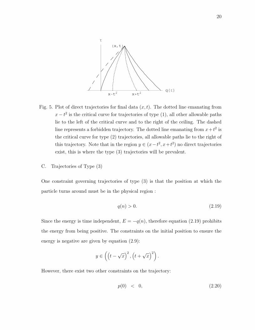
5 Plot of direct trajectories for final data (x, t). The dotted line

emanating from x− t2 is the critical curve for trajectories of type

(1), all other allowable paths lie to the left of the critical curve and

to the right of the ceiling. The dashed line represents a forbidden

trajectory. The dotted line emanating from x + t2 is the critical

curve for type (2) trajectories, all allowable paths lie to the right

of this trajectory. Note that in the region y ∈ (x − t2, x + t2) no

direct trajectories exist, this is where the type (3) trajectories will

be prevalent. . . . . . . . . . . . . . . . . . . . . . . . . . . . . . . . 20

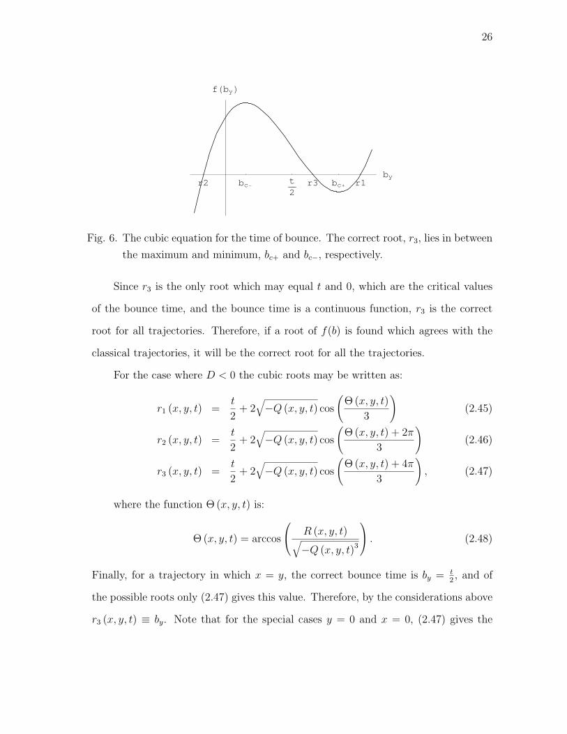
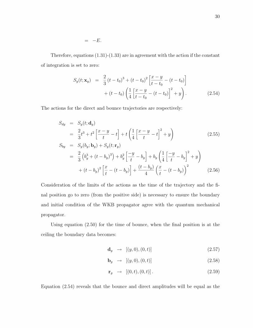
6 The cubic equation for the time of bounce. The correct root, r3,

lies in between the maximum and minimum, bc+ and bc−, respectively. 26

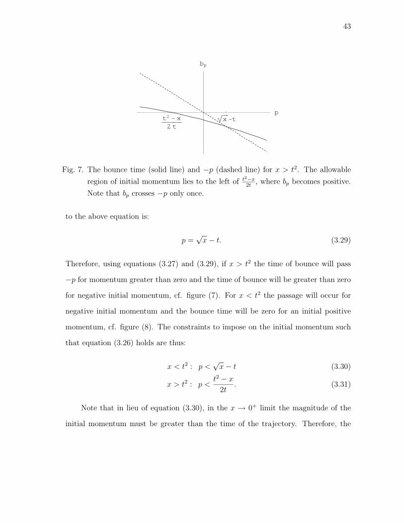
7 The bounce time (solid line) and −p (dashed line) for x > t2. The

allowable region of initial momentum lies to the left of t2−x2t

, where

bp becomes positive. Note that bp crosses −p only once. . . . . . . . . 43

x

FIGURE Page

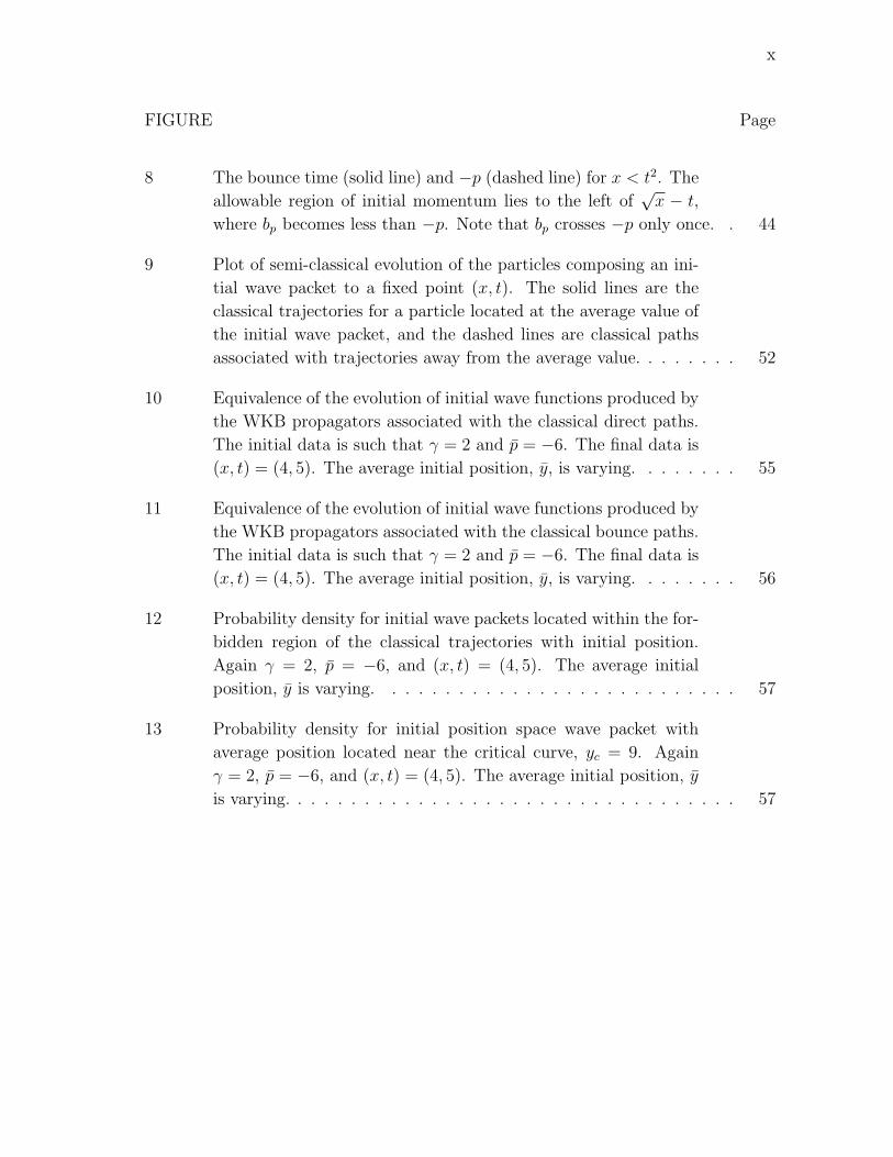
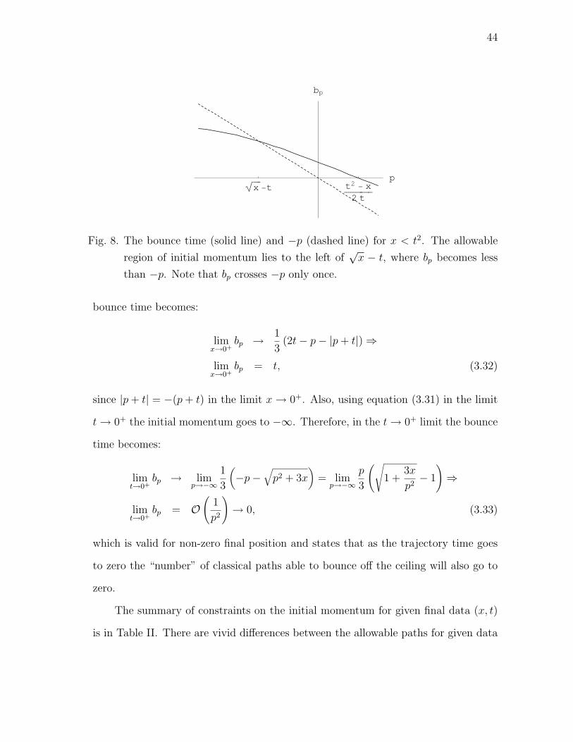
8 The bounce time (solid line) and −p (dashed line) for x < t2. The

allowable region of initial momentum lies to the left of√

x − t,

where bp becomes less than −p. Note that bp crosses −p only once. . 44

9 Plot of semi-classical evolution of the particles composing an ini-

tial wave packet to a fixed point (x, t). The solid lines are the

classical trajectories for a particle located at the average value of

the initial wave packet, and the dashed lines are classical paths

associated with trajectories away from the average value. . . . . . . . 52

10 Equivalence of the evolution of initial wave functions produced by

the WKB propagators associated with the classical direct paths.

The initial data is such that γ = 2 and p = −6. The final data is

(x, t) = (4, 5). The average initial position, y, is varying. . . . . . . . 55

11 Equivalence of the evolution of initial wave functions produced by

the WKB propagators associated with the classical bounce paths.

The initial data is such that γ = 2 and p = −6. The final data is

(x, t) = (4, 5). The average initial position, y, is varying. . . . . . . . 56

12 Probability density for initial wave packets located within the for-

bidden region of the classical trajectories with initial position.

Again γ = 2, p = −6, and (x, t) = (4, 5). The average initial

position, y is varying. . . . . . . . . . . . . . . . . . . . . . . . . . . 57

13 Probability density for initial position space wave packet with

average position located near the critical curve, yc = 9. Again

γ = 2, p = −6, and (x, t) = (4, 5). The average initial position, y

is varying. . . . . . . . . . . . . . . . . . . . . . . . . . . . . . . . . . 57

1

CHAPTER I

INTRODUCTION

Use of the ansatz

ψ(x, λ) = eiλ

S(x)∞∑

j=0

(i

λ)−jAj(x) (1.1)

λ → ∞

to solve differential equations has been in circulation since the mid-nineteenth century

[1]. In 1911 P. Debye used (1.1) for the solution of partial differential equations.

Soon after Debye’s work the physicists Wentzel, Kramers, Brillouin, and the English

mathematician Jeffreys used this technique to solve the Schrodinger equation

−h2

2m∇2ψ + V (~x)ψ = ih

∂ψ

∂t(1.2)

For this situation the parameter λ in (1.1) becomes Planc’s constant, h. The solutions

of the Schrodinger equation using the ansatz (1.1) are equivalent to the solutions of

the Feynman Kernel

K(x, t) =∫

D[x(t)] eih

S[x(t)] (1.3)

using the method of stationary phase [2]. For the propagator the WKB analysis is in

exact agreement with the analytic solutions corresponding to the free-particle, linear

potential and the quadratic potential [3]. However, the approximation is not exact

for the solution of the individual wave functions of (1.2) [4].

Application of (1.1) to the Schrodinger equation yields the Hamilton-Jacobi equa-

tion of classical mechanics in association with the lowest order of h. The corresponding

The journal model is IEEE Transactions on Automatic Control.

2

solution is the action, S[q(t)]. This solution depends on the trajectories, q(t), asso-

ciated with the classical situation requiring both initial and final data, not the usual

initial-value problem we encounter in undergraduate mechanics. However, in classi-

cal mechanics not all final data is accessible for trajectories with given initial data,

and the propagator associated with such “forbidden” regions will give no information

about the final probability. However, these regions may be accessible for given initial

momentum data. This type of behavior, where one representation is phase space

produces different results than another, is generally due to caustics ([5], [1]), or where

a caustic is the limiting case of the classical trajectories. Also, the solution to the

second lowest order equation in h (the “Amplitude”) generally develops singularities

by diverging as the classical trajectories pass a caustic[5]. Therefore, simply because

the WKB analysis with respect to certain initial data yields a null result does not

necessarily mean the propagator is also negligible. The WKB approximation cor-

responding to initial momentum and position data is therefore a logical analysis to

partake in, which is the main motivation of this thesis.

The remainder of the Introduction will discuss aspects of the classical system,

including the general constraints on a particle’s initial data given final position and

time. Explicit application of the WKB ansatz will follow, giving the equations gov-

erning the approximation to O(h), and a brief overview of Hamilton-Jacobi theory.

It also displays the analytic solution without derivation, and discusses the Fourier

transform relationship between the momentum and position space propagators.

The second and third chapters explicitly construct the approximations corre-

sponding to systems given initial position and momentum data, respectively. The

chapters also derive the classical equations of motion and the constraints on the clas-

sical paths.

The final chapter will compare the WKB propagators in the aforementioned

3

q

Linear Potential with Barrier¥

Ceiling

Fig. 1. The potential energy as a function of position. The ceiling is located at the

origin, the ∞ highlights the fact that the origin is impenetrable to the particle

(both classical and quantum).

“forbidden” region, and other cases of final data.

A. The Quantum and Classical System

The system considered in this paper is a particle confined to the positive region of a

one-dimensional coordinate system by means of an impenetrable barrier at the origin,

in the presence of a linear potential (cf. figure 1),

V (q) = −αq. (1.4)

Here q represents the position of the particle, and α characterizes the strength

and direction of the potential. For α greater than zero the barrier is a “ceiling” and

the particle may bounce off at most once. If α is less than zero then the barrier will

act as a floor, and will have, in principle, an infinite number of bounces. This paper

will consider only the ceiling case.

The Quantum theory of the system under consideration has the exact solution

4

in terms of the energy eigenfunctions u(x, E):

U(x, y, t) =∫ ∞

−∞e−

ih

Etu(x,E)u(y, E)ρ(E)dE, (1.5)

here u (x,E) and ρ (E) are:

u(x,E) = π[Ai

[λ

(−x− E

α

)]Bi

(−λ

E

α

)]

−π[Bi

[λ

(−x− E

α

)]Ai

(−λ

E

α

)](1.6)

ρ(E) =π−2

Ai2(−λE

α

)+ Bi2

(−λE

α

) (1.7)

λ ≡(

2mα

h2

) 13

. (1.8)

E is the energy eigenvalue of the system, t is the time of propagation, x and y are the

final and initial positions, respectively. This solution is a special case of the methods

considered in Dean and Fulling [6]. The evolution of an initial wave packet, ψ(y), is:

Ψ(x, t) =∫ ∞

−∞

∫ ∞

−∞e−

ih

Etψ(y)u(x,E)u(y, E)ρ(E)dEdy. (1.9)

The analytic solution for the propagator is difficult to use in obtaining probability

densities by numerical integration or other schemes. However, the WKB construction

is less problematic because it is representable in exact form, and integration schemes

(both numerical and analytic) to obtain probability densities are straight forward to

implement.

There are two types of classical trajectories to consider: those which will bounce

off the ceiling (bounce paths) and those which will not (direct paths). The latter

trajectories may either initially move toward the ceiling or initially move away, corre-

sponding to the initial momentum being less than or greater than zero, respectively.

This paper will consider the trajectories corresponding to two different types of initial

5

data:

• Initial momentum, p, and final position, x;

• Initial position, y, and final position, x.

The equation governing the dynamics of the classical system is:

d2q

dτ 2=

α

m⇒

q (τ) =α

2mτ 2 + Aτ + B. (1.10)

The constants of integration, A and B, are determined from the chosen initial con-

ditions. For bounce trajectories two solutions are required, q1 (τ) and q2 (τ), corre-

sponding to the dynamics before and after the collision, respectively. A third condi-

tion must be placed on the bounce trajectories such that the momenta of the paths

at the ceiling is equal in magnitude and opposite in direction. Letting b denote the

time at which the particle will ricochet, this condition is written as:

p1 (b) = −p2 (b) . (1.11)

Since the classical direct paths will never interact with the ceiling, the corre-

sponding WKB solutions for both types of data will be in agreement with the quan-

tum system corresponding to the Hamiltonian with a linear potential without the

boundary condition at the origin:

K−(x, y, t) =

√m

2πithe−iα2t3

24mh eiαt(x+y)

2h eim(x−y)2

2th (1.12)

K−(x, p, t) =1√2πh

e−i α2t3

6mh eih(p+αt)(x− pt

2m), (1.13)

(see [2] for equation 1.12). The only discrepancy is the WKB solutions carry con-

straints on the initial data to ensure the particle will not interact with the ceiling.

However, the WKB propagators corresponding to bounce trajectories will not yield

6

results identical to the analytic propagator. This is in contrast to the consensus that

the WKB approximation is exact for all potentials with at most quadratic form.

The remainder of the paper will use the following units:

h ≡ 1

m ≡ 1

2

α ≡ 1.

Note that in consequence of the above units, position will have the same dimension-

ality as time squared, and momentum will have the same dimensionality as time:

[x] = [t]2

[p] = [t].

B. The Classical Solutions

The preliminary quest is to determine all possible trajectories, q (τ), which obey

Hamilton’s equations connecting the initial data (p/y, t0) with the final data (x, t).

For notational simplicity the general data corresponding to the initial position and

initial momentum trajectories will be:

xy ≡ (y, t0), (x, t)

xp ≡ (p, t0), (x, t).

There are three types of non-bounce trajectories to consider:

1. Trajectories which initially and finally move away from the ceiling: p0 ∈ (0,∞),

and pf ∈ (0,∞)

2. Trajectories which initially and finally move toward the ceiling: p0 ∈ (−∞, 0),

7

y,xt xd1xd2q

t

Τ

Fig. 2. Three types of non-bounce trajectories with equal initial data, y, and final

time, t. The only variable is the final position, x. xd1 represents the final

position of a type (1) trajectory. xd2 is the final position for type (2). And xt

is for a turning trajectory, type (3).

and pf ∈ (−∞, 0)

3. Trajectories which initially move toward the ceiling, and end moving away from

the ceiling: p0 ∈ (−∞, 0), and pf ∈ (0,∞)

A plot of the three types of non-bounce trajectories is in figure (2). The time at which

the particle’s momentum is zero, n, governs the transition between motion toward

the ceiling and away from the ceiling for type (3) trajectories.

There are certain fundamental or “critical” trajectories which are helpful in an-

alyzing the more general situations. The critical trajectories of type (1) and (2) have

relationships with the case where the initial momentum of the particle is zero. For

given final data, (x, t), such a trajectory has initial position y ≡ x − t2, and the

trajectory is:

q(τ) = τ 2 + x− t2. (1.14)

Therefore, an initial relationship for this trivial case is that if x > t2 the initial

position will be on the physical side of the ceiling. Conversely, for x < t2 the initial

8

position will not be physical. Keeping the same final data implies that if an initial

positive momentum is given to this trajectory, the initial position must move towards

the ceiling. Conversely, for an initial negative momentum the initial position must

move away from the ceiling. Therefore, a general statement for the system (1.14)

corresponding to trajectories of type (1) and (2) is that as the particle is given initial

positive momentum the initial position must move away from the critical position, y,

and towards the ceiling. Whereas for the particle to have initial negative momentum

the initial position must move away from the critical position and away from the

ceiling,

Type(1) : y < y (1.15)

Type(2) : y > y. (1.16)

The linear potential implies that the momentum gained by the particle is equal

to the time of flight, τ , and the total momentum of the trajectory at any time is given

by:

τ + p0,

where p0 is the initial momentum of the trajectory. Therefore, the time at which the

particle will turn around is:

n = −p0. (1.17)

The “boundary” between cases (2) and (3) is analyzable in terms of the distance

traveled, ∆. For a trajectory where t = n:

∆ = −∫ n

0v(τ)dτ = −2

∫ −p0

0(p0 + τ) dτ ⇒

∆ = p20 = t2. (1.18)

9

y xq

t

b

Τ

Fig. 3. General direct (solid line) and bounce (dotted line) trajectory connecting initial

data, y, to the final data, x, in the same time, t.

The negative sign is placed in front of the integral because the velocity is inherently

negative. In accordance with y being the critical position for trajectories of type (1)

and (2), ∆ is the critical displacement for trajectories of type (3).

Some initial and final data characterize a non-bounce trajectory and a more

“energetic” bounce trajectory, cf. figure (3). The critical trajectory for the bounce

paths are the type (3) trajectories with zero momentum at the ceiling, corresponding

to zero energy, cf. figure (4). All subsequent trajectories for the bounce case will

have energy greater than zero (the proof follows in the subsequent chapters). A way

to view the construction of bounce trajectories is by joining two trajectories at the

ceiling which there obey equation (1.11). The trajectory prior to the bounce satisfies

the initial data, and the ricochet trajectory will satisfy the final data. The critical

trajectory for the bounce case is when these two trajectories are the same. A particle

in a linear potential beginning at the ceiling with zero energy (and therefore zero

initial momentum) will end at location x with momentum√

x. Conversely, if the

particle begins at y with zero energy then the momentum at the the ceiling will be

√y. Therefore, the total momentum the particle will gain for the critical bounce

10

y,xcceilingq

t

bc

Τ

Fig. 4. Generic family of bounce trajectories with the same initial position and final

time. The final position, x, is varying. The critical trajectory is dashed, and

bc denotes the time of bounce for this trajectory, xc denotes the final position.

trajectory is:

√x +

√y = t, (1.19)

where the equality to the total time is due to the fact that the particle will gain

momentum linearly with time.

C. The WKB Ansatz

The equations in this section will use h and m for notational clarity. The quantum

mechanical Hamiltonian operator, H, for the given system is:

H =p2

2m− q, (1.20)

11

where p and q are the momentum and position operators, respectively. Since the

Hamiltonian for the system is time-independent the time evolution operator is:

T (τ) ≡ e−ih

Hτ ,

where the initial time, t0, is set to zero. For the initial state, |α〉0, the time evolution

is:

T (t) |α〉0 .

In the position representation the evolution becomes:

〈q|α〉τ =∫

dy 〈q| T (t) |y〉 〈y|α〉0 (1.21)

=∫

dy U (q, y, τ) 〈y|α〉0. (1.22)

The quantity 〈q| T (τ) |y〉 ≡ U (q, y, τ) is the quantum mechanical propagator, and is

a solution to the time-dependent Schrodinger equation:

− h2

2m

∂2U

∂q2− qU = ih

∂U

∂τ, (1.23)

here the Hamiltonian (1.20) is in the configuration representation. Note that there

are two conditions the quantum mechanical propagator satisfies:

limτ→0

U (q, y, τ) = limτ→0

〈q| T (τ) |y〉 ≡ δ(q − y), (1.24)

U(0, y, t) = 0. (1.25)

The initial condition is specific to the configuration representation, while the bound-

ary condition is general and due to the impenetrable barrier at the origin. The WKB

ansatz requires assuming the propagator for times τ > 0 will be:

U(q, τ) ∼ A(q, τ) eih

S(q,τ). (1.26)

12

Inserting this representation into equation (1.23) and making a formal series expansion

in powers of h yields, to order h0:

1

2m

(∂S(q, τ)

∂q

)2

+ V (q) +∂S(q, τ)

∂τ= 0, (1.27)

which is the Hamilton-Jacobi (HJ) equation of classical mechanics [7]. The solution

is known as “Hamilton’s principal function”, or the action. The solution to the HJ

equation will admit a family of trajectories, q (τ, α), where α specifies the initial and

final data. For the present problem α is such that q (t) = x. Because the Hamiltonian

does not depend on the time, the relationship between the action and the energy:

E = −∂S

∂τ(1.28)

is valid. The main characteristic of the action is its derivative with respect to position:

p(q) =∂S

∂q. (1.29)

A similar relationship for the case where the trajectory is given initial momentum is:

∂S

∂p= y. (1.30)

This paper will use the evaluation of equations (1.29) and (1.28) for τ = t, and

(1.30) check the validity of the actions in the following chapters:

∂S

∂x= p(t), (1.31)

∂S

∂t= −E, (1.32)

∂S

∂p= y. (1.33)

The total time derivative of the action is the Lagrangian of the system, L(q, q, τ).

Therefore, if the trajectories are already known the construction of the action is the

13

indefinite time integral of the system Lagrangian with a constant of integration to

satisfy (1.31)-(1.33):

S (q, τ) =∫

L (q, q, τ) dτ + C. (1.34)

For trajectories interacting with the ceiling the separate indefinite time integrals of

the Lagrangians corresponding to each trajectory before and after the bounce yields

the action up to a constant:

Sb (q, τ) =∫

L(q1, q1, τ)dτ +∫

L (q2, q2, τ) dτ + C. (1.35)

Again, the constant of integration ensures the validity of equations (1.31)-(1.33).

To the order h1 substitution of the WKB ansatz into the time-dependent Schrodinger

equation yields:

∂q [A(q, τ) p(τ)] + p(τ) ∂qA(q, τ) = −∂τA(q, τ), (1.36)

again equation (1.29) defines p(τ). Defining the density function ρ(q, τ) ≡ |A(q, τ)|2,the amplitude equation becomes [5]:

∂τρ(q, τ) = −∂q{ρ(q, τ) v(τ)}, (1.37)

where v(τ) = p(τ)m

= 2 p(τ). The quantity ρ (q, τ) has the interpretation of a density of

classical particles in the N-dimensional subspace spanned by q of the 2N dimensional

phase-space such that the number of particles between q and q+dq is ρ (q, τ) dq. Note

that the subspace describing the density is not necessarily position as a function of

momentum, but is any set of canonical variables. The total number of particles at

time τ in the subspace spanned by q is:

N (τ) =∫

dq ρ (q, τ) ,

14

which remains constant for all values of time. Therefore, the Jacobian representing

the change in canonical coordinates from q1 (τ1) to q2 (τ2) governs the evolution of the

density function:

ρ (q2, τ2) = ρ (q1, τ1)

∣∣∣∣∣∂q1

∂q2

∣∣∣∣∣ . (1.38)

Therefore, the transformation of the amplitude function is in general:

A (r) = A (u) |J (r,u)| 12 , (1.39)

here u represents the initial representation describing the the density function and r

is the final. The determination of the initial amplitude, A(u), is such that the WKB

propagator agrees with the correct analytic propagator initially and at the ceiling,

equations (1.24) and (1.25) respectively.

Therefore, the general form of the WKB propagator with initial data y and final

data (x, t) to O(h) is:

K (x, y, t) = A (u) |J (r,u)| 12 eih

S(x,y,t). (1.40)

Here the explicit dependence of the action on the initial parameter y reveals the

propagator acts on states initially in configuration space. However, since the initial

position is a parameter the Jacobian in equation (1.39) will diverge for all final data

if the initial density of classical particles is given in the position representation of

phase space. To avoid this divergence the characterization of the initial density is in

the momentum subspace, and the final representation is in position.

The relationship between the quantum mechanical propagators with initial posi-

tion data, 〈x| T (τ) |y〉 = U (q, y, τ), and that with initial momentum data, 〈x| T (τ) |p〉 =

15

U (q, p, τ) is:

〈q|α〉τ =∫ ∞

−∞dy 〈x| T (t) |y〉 〈y|α〉0

=∫ ∞

−∞dp 〈x| T (t) |p〉 〈p|α〉0, (1.41)

where 〈p|α〉0 is the Fourier transform of the initial state vector:

〈p|α〉0 =∫ ∞

−∞dy 〈p|y〉〈y|α〉0

=1√2πh

∫ ∞

−∞dy e−

ih

py〈y|α〉0.

This relationship is valid for the WKB approximations also. However, the constraints

on the initial data due to the classical considerations will not allow the integration

ranges in (1.21) and (1.41) to cover all possible values. If the regions the classical

constraints do not allow integration over correspond to regions where the quantum

mechanical propagator oscillates violently or has high damping then the approxima-

tion should be accurate. The construction of the WKB propagator corresponding to

trajectories given initial momentum data is identical to the initial position construc-

tion. Inconsistencies arise from the difference in the constraints on the initial data

and the form of the action. In contrast to equation (1.24), the initial form of the

propagator with initial momentum data is:

limτ→0

U(x, p, τ) = limτ→0

⟨x

∣∣∣T (τ)∣∣∣ p

⟩≡ e

ih

xp

√2πh

. (1.42)

And it is this condition which the initial amplitudes must generate for the initial

momentum case, as well as equation (1.25).

16

CHAPTER II

TRAJECTORIES WITH GIVEN INITIAL POSITION DATA

Throughout this chapter the denotation of initial, (p, t0), and final data, (x, t), is:

dy ≡ [(p, 0), (x, t)]

by ≡ [(p, 0), (0, by)]

ry ≡ [(−p− by, by), (x, t)] ,

here by denotes the time of bounce for trajectories given initial position data.

Using equation (1.10), the general trajectory and momentum connecting the

initial data (y, t0) to the final data (x, t) for the linear potential are:

q(τ ;xy) = (τ − t0)2 + (τ − t0)

[x− y

t− t0− (t− t0)

]+ y (2.1)

p(τ ;xy) = (τ − t0) +1

2

[x− y

t− t0− (t− t0)

]. (2.2)

For the direct path t0 → 0 in xy, and the trajectory and momentum are:

q(τ ;dy) = τ 2 + τ[x− y

t− t

]+ y (2.3)

p(τ ;dy) = τ +1

2

(x− y

t− t

). (2.4)

Note that equation (2.4) implies that the trajectory with initial momentum equal to

zero will have an initial position given by:

y = x− t2, (2.5)

in agreement with the arguments of the introduction.

17

The Hamiltonian of the non-bounce trajectories is given by:

Hy,d = p(t)2 − x =1

4t2

(y2 − 2y

(t2 + x

)+ (x− t2)2

), (2.6)

and the constraints on the energy being positive or negative are thus:

Hy,d > 0 : y ∈(−∞,

(t−√x

)2)∪

((t +

√x

)2,∞

)(2.7)

Hy,d = 0 : y =(t±√x

)2(2.8)

Hy,d < 0 : y ∈((

t−√x)2

,(t +

√x

)2)

. (2.9)

Using equations (2.2) and (2.1) the trajectories and momenta for the bounce

paths are:

q(τ ;by) = τ 2 − τ(b +

y

b

)+ y (2.10)

q(τ ; ry) =(τ 2 − t2

)+

τ − t

b− t

(−

(b2 − t2

)− x

)+ x (2.11)

p(τ ;by) = τ −(

y

2b+

b

2

)(2.12)

p(τ ; ry) = τ − 1

2

(x

b− t+ (b + t)

), (2.13)

and the corresponding Hamiltonian is:

Hy,b = p1(b)2 =

(b2 − y)2

4b2. (2.14)

Using equations (1.17) and (2.4), the time at which the particle will turn-around,

ny, is:

ny = −p0 = −(

x− y

2t− t

2

)⇒

ny =1

2

(y − x

t+ t

). (2.15)

18

A. Trajectories of Type (1)

Since the potential drives the particle away from the ceiling, the final momentum of

a particle initially moving away from the ceiling will also be positive, therefore the

only constraint to impose on trajectories of type (1) is:

p (0) > 0 ⇒ y < x− t2 = y, (2.16)

which describes the fact that as the initial momentum of the particle is positively

increased from zero the initial position will be pushed away from the limiting value,

y. However, as noted in the introduction, in order to ensure that y > 0, it must be

that x > t2. Therefore the correct constraint is:

x > t2 : y < x− t2. (2.17)

Note that t2 ⇒ αt2

2m, which is the displacement of a particle with zero initial velocity.

Therefore, requiring x − y > t2 implies there must be an initial positive momentum

to alow the particle to reach the final destination within time t. Therefore, the

conflict arising which constrains the the final data is that for given (x, t) as the initial

momentum is increased the initial position must be set closer to the ceiling, and the

limiting case is y = 0 ⇒ x = t2.

The energy of the direct trajectory may be negative or positive. From equations

(2.7) and (2.9) the energy of the direct trajectories may be divided into:

E > 0 : y ∈(0,

(√x− t

)2)

E < 0 : y ∈((√

x− t)2

, x− t2)

.

19

B. Trajectories of Type (2)

If a trajectory initially and finally moves toward the ceiling then the momentum

gained during flight, t, must be less than the momentum to turn the particle around,

t < ny, using equation (2.15) reveals:

y > x + t2. (2.18)

Since the particle will not turn around it will travel a total distance ∆ = y − x.

Therefore equation (2.18) states that the total distance for the direct trajectory is

greater than the minimum turning trajectory distance, implying the necessity of an

initial negative momentum, cf. (1.18). Unlike (2.17) there is no constraint on the

relationship between the final data (x, t). This is because for given final data (x, t),

as the initial momentum increases negatively the initial position will move away from

the non-physical region, not towards. Therefore, the positivity requirement on x and

t is enough to ensure that the trajectory will not pass into the forbidden region, for

initial negative momentum.

Finally, note that the energy may again be positive or negative depending on the

relationship between y and (x, t):

E < 0 : y ∈(x + t2,

(√x + t

)2)

E > 0 : y ∈((√

x + t)2

,∞)

20

x-t2 x+t2qHΤL

Τ

Hx,tL

Fig. 5. Plot of direct trajectories for final data (x, t). The dotted line emanating from

x− t2 is the critical curve for trajectories of type (1), all other allowable paths

lie to the left of the critical curve and to the right of the ceiling. The dashed

line represents a forbidden trajectory. The dotted line emanating from x+ t2 is

the critical curve for type (2) trajectories, all allowable paths lie to the right of

this trajectory. Note that in the region y ∈ (x− t2, x+ t2) no direct trajectories

exist, this is where the type (3) trajectories will be prevalent.

C. Trajectories of Type (3)

One constraint governing trajectories of type (3) is that the position at which the

particle turns around must be in the physical region :

q(n) > 0. (2.19)

Since the energy is time independent, E = −q(n), therefore equation (2.19) prohibits

the energy from being positive. The constraints on the initial position to ensure the

energy is negative are given by equation (2.9):

y ∈((

t−√x)2

,(t +

√x

)2)

.

However, there exist two other constraints on the trajectory:

p(0) < 0, (2.20)

21

t > ny. (2.21)

Using (2.4) and (2.15) these constraints collectively imply:

y ∈(x− t2, x + t2

)⇒

y ∈((√

x− t) (√

x + t),(t +

√x

)2 − 2t√

x)

. (2.22)

Comparing (2.9) and (2.22), the upper bound on the initial position is:

y < x + t2,

and the two possible lower bounds on y are:

(√x− t

) (√x + t

), (2.23)

(√x− t

) (√x− t

). (2.24)

If√

x < t then Eq.(2.23) is negative and hence the lower bound for y is Eq.(2.24).

For√

x > t both bounds will be positive, but since√

x − t <√

x + t, Eq.(2.24) is

the proper lower bound. Since whether√

x is greater or less than t does not affect

the upper bound, the constraints on the initial position for a trajectory which turns

around are:

√x < t : (

√x− t)2 < y < x + t2 (2.25)

√x > t : x− t2 < y < x + t2. (2.26)

Figure (5) gives a graphical representation of the direct trajectories.

22

D. Bounce Trajectories

Using equations (2.12) and (2.13) for the requirement that the initial and final mo-

mentum be less than and greater than zero, respectively, yields the equations:

p(0;by) < 0 ⇒ −1

2

(y

by

+ by

)< 0 (2.27)

p(t; ry) > 0 ⇒ 1

2

(x

t− by

− (t− by)

)> 0 ⇒ x > − (t− b)2 . (2.28)

Therefore, the constraints of positivity on the parameters (x, y, t) are enough such

that the momentum requirements of the trajectories have no implications. Also,

equation (2.14) implies that the energy of the bounce trajectory must be positive,

with the limiting value of zero. The general constraint on the positivity of the bounce

Hamiltonian is thus:

Hy,b =1

4b2y

(b4y + y2 − 2b2

yy)

> 0 ⇒(b2y − y

)2> 0,

therefore the general energy requirement on the trajectory also has no bearing. How-

ever the limiting bounce trajectory is identical with the turning point trajectory

corresponding to the same energy:

Hy,d =1

4t2

(y2 − 2y

(t2 + x

)+

(t2 − x

)2)

= 0 ⇒

y =(t±√x

)2.

Comparing this result with the inequality in equation (2.25), the correct root is

(t−√x)2. Therefore on the critical bounce trajectory the relationship between the

parameters is:

√y +

√x = t, (2.29)

23

which agrees with equation (1.19). For given final data, increasing the momentum

at the ceiling from zero will require the particle to move to the final position in a

time less than that of the critical trajectory,√

x. Therefore, to not alter the final

data the initial position will move away from the ceiling, and hence increase√

y. The

governing constraint on the bounce trajectories is therefore:

√x +

√y ≥ t. (2.30)

The ceiling condition for the bounce trajectory, q1 (b) = −q2 (b), yields the equa-

tion:

f (b) ≡ b3 + a2b2 + a1b + a0 = 0 (2.31)

a2 ≡ −3

2t (2.32)

a1 ≡ t2

2− 1

2(x + y) (2.33)

a0 ≡ yt

2. (2.34)

The polynomial discriminant of the cubic equation, D, is defined as [8]:

D ≡ R2 + Q3 =

t2

64

((x− y)2 − 4

9(x + y)2

)−

(t2

12

)3

−(

1

6(x + y)

)3

− t4

288(x + y) , (2.35)

where the definitions of R and Q are:

Q =3a1 − a2

2

9= − t2

12− 1

6(x + y) (2.36)

R =9a1a2 − 27a0 − 2a3

2

54=

t

8(x− y) . (2.37)

If D > 0 then one root will be real and the other two are complex conjugates,

D = 0 if all roots are real and at least two are equal, and D < 0 for all roots being

24

real and unequal. From equation (2.35):

D(t = 0) < 0 (2.38)

limt→∞D(t) = −∞. (2.39)

To analyze the discriminant’s behavior as t →∞ let T ≡ t2, then:

dD

dT=

1

64

((x− y)2 − 4

9(x + y)2

)−

(T

24

)2

− T

144(x + y) . (2.40)

Therefore, the derivative of the discriminant will tend to −∞ as t →∞ . Setting the

above equation to zero reveals the character of the critical points of the polynomial

discriminant:

T 2 + 4 (x + y) T − 9((x− y)2 − 4

9(x + y)2

)= 0 ⇒ (2.41)

±√

(x (−2± 3)− y (2± 3)) = t.

The two negative roots are not physical, therefore the only possible critical points

are:

tc+ =√

x− 5y

tc− =√

y − 5x.

Since the discriminant is initially less than zero and moves toward −∞, if the initial

and final data do not satisfy x > 5y or y > 5x then the derivative of the discriminant

will always be negative and hence so will the discriminant. If the final data does

satisfy one of the above inequalities then only one of the positive roots will be real.

Without loss of generality assume x > 5y, therefore the root of equation (2.42) is tc+.

Furthermore, equations (2.38) and (2.39) imply that this root must be a maximum

for D(t). Therefore, if D(tc+) < 0 then the polynomial discriminant will be negative

25

for all values of t. Using equation (2.35):

D(tc+) =1

64

((x− 5y) (x− y)2 − (x− y)3

).

Which implies the discriminant will always be negative if:

((x− 5y) (x− y)2 − (x− y)3

)< 0 ⇒

x− 5y < x− y ⇒

0 < 4y.

Therefore, provided that y 6= 0, D(t) < 0 for all t and all three roots to equation

(2.31) are real and unequal. Similarly, if y > 5x then the requirement that D(t) < 0

is 0 < x, which is in general true except for the special case x = 0. The special cases

y = 0 and x = 0 respectively imply that the initial and final positions are at the

ceiling, and the time of bounce should respectively be 0 and t.

The maximum and minimum of the cubic equation are:

df (b)

db= 0 ⇒

bc± =t

2±

√t2

12+

1

6(x + y),

and the point at which the equation changes its concavity is t2. Since b → ±∞ ⇒

f(b) → ±∞ the point bc− is where f(b) changes from being concave to convex. Since

all three roots must be real one root of f(b) will lie between the two extremum, and

the other two must lie outside of the range (cf. figure (6)):

r1 ∈ (−∞, bc−) (2.42)

r2 ∈ (bc+,∞) (2.43)

r3 ∈ (bc−, bc+) . (2.44)

26

bc+bc- t����

2r1r2 r3

by

fHbyL

Fig. 6. The cubic equation for the time of bounce. The correct root, r3, lies in between

the maximum and minimum, bc+ and bc−, respectively.

Since r3 is the only root which may equal t and 0, which are the critical values

of the bounce time, and the bounce time is a continuous function, r3 is the correct

root for all trajectories. Therefore, if a root of f(b) is found which agrees with the

classical trajectories, it will be the correct root for all the trajectories.

For the case where D < 0 the cubic roots may be written as:

r1 (x, y, t) =t

2+ 2

√−Q (x, y, t) cos

(Θ (x, y, t)

3

)(2.45)

r2 (x, y, t) =t

2+ 2

√−Q (x, y, t) cos

(Θ (x, y, t) + 2π

3

)(2.46)

r3 (x, y, t) =t

2+ 2

√−Q (x, y, t) cos

(Θ (x, y, t) + 4π

3

), (2.47)

where the function Θ (x, y, t) is:

Θ (x, y, t) = arccos

R (x, y, t)√

−Q (x, y, t)3

. (2.48)

Finally, for a trajectory in which x = y, the correct bounce time is by = t2, and of

the possible roots only (2.47) gives this value. Therefore, by the considerations above

r3 (x, y, t) ≡ by. Note that for the special cases y = 0 and x = 0, (2.47) gives the

27

correct values:

r3(x, 0, t) = 0 (2.49)

r3(0, y, t) = t. (2.50)

Note that to leading order, the limit of the time of bounce as t → 0+ is:

limt→0+

by =y t

x + y, (2.51)

this equation will be prevalent when considering the asymptotic behavior of the action

and amplitude.

The summary of constraints on the initial position are given in Table I. The

allowable paths for initial and final data (y, x, t) are deducible from the table by

organizing the final data into two categories:

1. x ∈ (t2,∞)

2. x ∈ (0, t2).

Note that the direct path (p0 < 0) belongs to both categories.

Considering category (1), both direct paths and the turning path constrain the

initial position into mutually exclusive intervals:

• y ∈ (0, x− t2)

• y ∈ (x− t2, x + t2)

• y ∈ (x + t2,∞).

Therefore, for x ∈ (t2,∞) only one of the above paths is possible. However, the region

for the bounce trajectories, y ∈ ((√

x− t)2,∞), is within each of the above allowable

non-bounce regions.

28

For x ∈ (0, t2), the other turning path and the direct path (p0 < 0) again

constrain y into the respective mutually exclusive intervals:

• y ∈ ((√

x− t)2, x + t2)

• y ∈ (x + t2,∞),

the bounce interval is also within these intervals.

Therefore, there are at most two allowable trajectories for given initial and final

data, the bounce path and one non-bounce. However, if a bounce path does not exist

then according to equation (2.30):

√x +

√y < t

⇒ y ∈ (0, (t−√x)2).

This region of initial position data is explicitly exclusive from all the possible tra-

jectories except the direct (p0 > 0) trajectory. However, since the direct (p0 > 0)

trajectory is only valid for x ∈ (t2,∞), the interval of initial data becomes imaginary,

√y < t − √

x < 0, which is physically impossible. In conclusion there will always

be either one bounce path and one non-bounce path(√

y +√

x > t), or no possi-

ble paths(√

y +√

x < t), for given initial and final data (y, x, t). Note that in the

limiting case,√

y +√

x = t, the bounce path and non-bounce path are identical.

E. The Classical Action

The complete WKB construction requires the determination of the action of the

trajectories and the amplitude function. Using equations (2.1) and (2.2) the general

Lagrangian for the initial position formulation is:

L [q, q, τ ] = p(τ ;xy)2 + q(τ ;xy)

29

Table I. Constraints on the initial position with final data. The inequalities were

checked using Mathematica.

x ∈ y ∈ Trajectory

(t2,∞) (0, x− t2) Direct, p0 > 0

(0,∞) (x + t2,∞) Direct, p0 < 0

(0, t2)((√

x− t)2, x + t2

)Turning

(t2,∞) (x− t2, x + t2) Turning

(0,∞)((t−√x)

2,∞

)Bounce

= 2 (τ − t0)2 + 2 (τ − t0)

[x− y

t− t0− (t− t0)

]

+1

4

[x− y

t− t0− (t− t0)

]2

+ y. (2.52)

And using (1.34), the action of the most general trajectory for time τ = t, up to the

constant of integration, is:

Sy(t;xy) =∫ t

dτ L [q, q, τ ] + C

=2

3(t− t0)

3 + (t− t0)2

[x− y

t− t0− (t− t0)

]

+ (t− t0)

(1

4

[x− y

t− t0− (t− t0)

]2

+ y

)+ C. (2.53)

The partial derivatives of (2.53) with respect to the final position and time are re-

spectively:

∂Sy(x)

∂x= (t− t0) +

1

2

[x− y

t− t0− (t− t0)

]

= p(t;x),

∂Sy(x)

∂t= x + p(0,x)2 − (t− t0)

2 + 2(t− t0) p(0;x)∂p(0;x)

∂t

= −(t− t0)2 − p(0;x)2 − 2p(0;x)(t− t0) + x

30

= −E.

Therefore, equations (1.31)-(1.33) are in agreement with the action if the constant

of integration is set to zero:

Sy(t;xy) =2

3(t− t0)

3 + (t− t0)2

[x− y

t− t0− (t− t0)

]

+ (t− t0)

(1

4

[x− y

t− t0− (t− t0)

]2

+ y

). (2.54)

The actions for the direct and bounce trajectories are respectively:

Sdy = Sy(t;dy)

=2

3t3 + t2

[x− y

t− t

]+ t

(1

4

[x− y

t− t

]2

+ y

)(2.55)

Sby = Sy(by;by) + Sy(t; ry)

=2

3

(b3y + (t− by)

3)

+ b2y

[−y

t− by

]+ by

(1

4

[−y

t− by

]2

+ y

)

+ (t− by)2

[x

t− (t− by)

]+

(t− by)

4

(x

t− (t− by)

)2

(2.56)

Consideration of the limits of the actions as the time of the trajectory and the fi-

nal position go to zero (from the positive side) is necessary to ensure the boundary

and initial condition of the WKB propagator agree with the quantum mechanical

propagator.

Using equation (2.50) for the time of bounce, when the final position is at the

ceiling the boundary data becomes:

dy → [(y, 0), (0, t)] (2.57)

by → [(y, 0), (0, t)] (2.58)

ry → [(0, t), (0, t)] . (2.59)

Equation (2.54) reveals that the bounce and direct amplitudes will be equal as the

31

final data moves toward the ceiling:

limx→0+

Sby = Sdy. (2.60)

Together with the amplitude (see the next section) this condition will ensure that the

WKB propagator will vanish for x = 0.

The leading order term of the general action in the limit as t → t+0 is:

limt→t+0

Sy(t;xy) =(x− y)2

4(t− t0)+O(t− t0). (2.61)

Using equation (2.54) and (2.51) for the limit of the bounce time, the limits of the

WKB phases as time goes to zero are:

limt→0+

Syd =(x− y)2

4t+O(t) (2.62)

limt→0+

Syb =y(x + y)2

4xt+O(t). (2.63)

The WKB phase for the direct path exhibits the correct delta function behavior

as x → y. Whereas the bounce phase will create violent oscillations in the WKB

propagator in the t → 0+ limit, with an effective contribution of zero upon integration

of an initial wave function.

Note that when considering bounce trajectories the partial derivative operators

must take the functional dependence of the time of bounce into account, e.g. :

∂

∂x→ ∂

∂x+

∂by

∂x

∂

∂by

. (2.64)

Therefore, applying a partial derivative operator to the action for the bounce trajec-

tories results in the extra term:

∂

∂by

[Sy(by;by) + Sy(t; ry)] . (2.65)

32

However, equation (2.54) shows that the partial derivative of the general action with

respect to the initial time, t0, is opposite the derivative with respect to the final time:

∂Sy(t;xy)

∂t0= −∂Sy(t;xy)

∂t

= E.

Since by is the final time for Sy(by;by) and the initial time for Sy(t; ry), it follows that

equation (2.65) is zero.

F. The Amplitude

Since the initial and final position are parameters for this problem the Jacobian

in equation (1.38) is undefined. However, using the momentum representation to

initially describe the amplitude implies the Jacobian,∣∣∣∂p(0;xy)

∂x

∣∣∣, is valid for trajectories

with initial position data:

Af (x, y, t) = A0 (x, y, t)

√√√√∣∣∣∣∣∂p (0;xy)

∂x

∣∣∣∣∣. (2.66)

Using equation (2.4), the Jacobian corresponding to the direct amplitude yields:

∂p(0;dy)

∂x=

1

2t. (2.67)

Requiring the initial form of the WKB propagator to agree with the initial form of

the quantum mechanical propagator, δ(y − x), yields the initial amplitude:

limt→0

Ad0√2t

eiSd(x,y,t) = limt→0

Ad0√2t

e(y−x)2

4it = Ad0

√2πi δ (y − x) ⇒

Ad0 =1√2πi

,

33

here equation (2.62) gives the correct form of the direct phase in the t → 0+ limit.

Therefore, the amplitude function for the direct path is given by:

Ad(t) =1√4πit

. (2.68)

Note that in lieu of equation (2.63), the t → 0+ limit of the bounce part of the WKB

propagator will make no contribution with respect to integration over an initial wave

function. This corresponds to the fact that as t → 0+ the number of possible classical

bounce trajectories goes to zero. Therefore the amplitude corresponding to the direct

propagator is all that is necessary to ensure the equivalence of the WKB propagator

and the exact quantum mechanical form in the t → 0+ limit.

Using by from equation (2.47), and p1 (0) from equation (2.12), the Jacobian

corresponding to the action for the bounce case is given by:

∂p (0;by)

∂x=

(y

2b2y

− 1

2

)∂by

∂x

=

(y

2b2y

− 1

2

)

×cos

(Θ+4π

3

)

6√−Q

[1− Q

6√−D

(t

2+

R

Q4

)tan

(Θ + 4π

3

)]. (2.69)

However, linearizing the classical equations of motion for the potential V = − |q|, and

then “folding” the negative half of the axis onto the positive half produces a more

explicit form of the Jacobian. For the given potential:

−∂V

∂q= sgn (q) = 2Θ (q)− 1, (2.70)

and Θ (q) is the Heavyside step function. Differentiating (2.70) with respect to a

parameter, α, yields:

∂

∂α[2Θ (q)− 1] = 2δ (q) = 2

δ (τ − by)

|q (by)|∂q

∂α. (2.71)

34

Note that using equation (2.12) along with the fact that p (by) < 0 for the bounce

trajectory moving toward the ceiling:

|q (by)| = y

by

− by. (2.72)

Therefore, differentiating Hamilton’s equations with respect α ≡ y yields:

d

dτ

∂p

∂y= 2

δ (τ − by)

|q (by)|∂q

∂y(2.73)

d

dτ

∂q

∂y= 2

∂p

∂y. (2.74)

For the trajectory moving toward the ceiling, τ < by, equation (2.73) predicts:

d

dτ

∂p

∂y= 0,

so that ∂p∂y

is a constant. Therefore, defining ∂p∂y

(0) ≡ C implies:

∂p

∂y(τ) = C (2.75)

for τ < by. The solution to (2.74) for τ < by is:

∂q

∂y= 2Cτ + 1, (2.76)

since q(0) = y ⇒ ∂q∂y

(0) = 1. Integrating (2.73) for τ > by, and using equation (2.72)

yields:

∂p

∂y= C +

2

|q (by)|∂q

∂y(by)

=C

[y + 3b2

y

]+ 2by

y − b2y

. (2.77)

And using this result for ∂q∂y

yields:

∂q

∂y(τ) =

∂q

∂y(by) + 2

∂p

∂y

∫ t

by

dτ

35

= (2 C by + 1) + 2C

[y + 3b2

y

]+ 2by

y − b2y

(t− by) .

Since q(t) = x it follows that ∂q∂y

(t) = 0. Therefore, after algebraic manipulations, the

constant C = ∂p∂y

(0) is:

∂p

∂y(0) =

1

2

5b2y − 4tby − y(

y − b2y

)b + (t− by)

(y + 3b2

y

) . (2.78)

Finally, using this result in (2.77) and the cubic equation (2.31) to simplify the de-

nominator, the sought after Jacobian is:

−∂p

∂y(t) =

b2y − y

2[−3tb2

y + 2 (t2 − x− y) by + 3yt] , (2.79)

The minus sign is accountable for the change in the direction of the momentum due

to the “folding” of the negative-half axis over, i.e. creating the ceiling.

The initial amplitude function for the bounce trajectories is chosen such that the

WKB propagator vanishes at the ceiling, Uy(0, y, t) = 0. From equations (2.63) and

(2.62) the phases of the direct and bounce parts of the propagator are identical in

this limit. Therefore, the initial amplitude for the bounce case must be such that in

the x → 0+ limit the amplitudes are opposite:

limx→0+

Ayb(x, y, t) = −Ayd(t) =−1√4πit

. (2.80)

Using (2.50) for the limit of the bounce time, the Jacobian for the bounce paths

becomes:

limx→0+

∣∣∣∣∣∣b2y − y

2[−3tb2

y + 2 (t2 − x− y) by + 3yt]∣∣∣∣∣∣

12

=1√2t

, (2.81)

36

therefore the appropriate initial amplitude is −1√2πi

:

Ayb =−1√2πi

∣∣∣∣∣∣b2y − y

2[−3tb2

y + 2 (t2 − x− y) by + 3yt]∣∣∣∣∣∣

12

. (2.82)

Since the critical curve for the bounce path is identical with the trajectory of type

(3) for E = 0, the relationship between the initial position and by is:

y = b2y, (2.83)

on the critical curve. Therefore, the amplitude for the bounce path will vanish on the

critical curve, agreing with classical consideratons.

Putting everything together, the WKB propagators for the direct and bounce

cases are respectively:

Uyd (x, y, t) =exp

[i(

23t3 + t2

[x−y

t− t

]+ t

(14

[x−y

t− t

]2+ y

))]

√4πit

, (2.84)

Uyb (x, y, t) =−1√2πi

∣∣∣∣∣∣b2y − y

2[−3tb2

y + 2 (t2 − x− y) by + 3yt]∣∣∣∣∣∣

12

× exp

[i

(2

3b3y + b2

y

[−y

t− by

]+ by

(1

4

[−y

t− by

]2

+ y

))]

× exp[i(

2

3(t− by)

3 + (t− by)2

[x

t− (t− by)

])]

× exp

[i(t− by)

4

(x

t− (t− by)

)2]. (2.85)

Note that, with the exception of the constraints on the initial position, the prop-

agator for the direct paths is identical with that for the linear potential without a

ceiling (1.12).

37

CHAPTER III

TRAJECTORIES WITH GIVEN INITIAL MOMENTUM DATA

Throughout this chapter the denotation of initial, (p, t0), and final data, (x, t), is:

dp ≡ [(p, 0), (x, t)]

bp ≡ [(p, 0), (0, bp)]

rp ≡ [(−p− bp, bp), (x, t)]

The general classical path and the corresponding momentum connecting the

initial data (p, t0) with final data (x, t) are:

q(τ ;xp) = (τ − t)2 + 2 (τ − t) (p + t− t0) + x (3.1)

p(τ ;xp) = (τ − t0) + p. (3.2)

The general Hamiltonian of the classical system is therefore:

H(τ ;xp) = (t− t0 + p)2 − x. (3.3)

The position and momentum for the non-bounce case are:

q(τ ;dp) = (τ − t)2 + 2(τ − t) (p + t) + x (3.4)

p (τ ;dp) = τ + p, (3.5)

and the Hamiltonian for the direct case is:

Hp,d = (p + t)2 − x = p2 + 2pt + t2 − x, (3.6)

The categories for the energy of the direct trajectories are:

Hp,d > 0 : p ∈(−∞,−√x− t

)∪

(√x− t,∞

)(3.7)

38

Hp,d = 0 : p = ±√x− t (3.8)

Hp,d < 0 : p ∈(−√x− t,

√x− t

). (3.9)

Using equation (3.1) the bounce paths are:

q (τ ;bp) = (τ − bp)2 + 2 (τ − bp) (p + bp) (3.10)

q (τ ; rp) = (τ − t)2 + 2 (τ − t) (t− bp − 2p) + x, (3.11)

and the momenta of the bounce trajectories are:

p(τ ;bp) = τ + p (3.12)

p(τ ; rp) = (τ − bp)− (bp + p) . (3.13)

The Hamiltonian for the bounce trajectories is thus:

Hp,b = p(bp;bp)2 = (p + bp)

2 . (3.14)

Note that the bounce Hamiltonian is always greater than or equal to zero, with

equality for p = −bp.

Since all must stay on the positive side of the ceiling, a general constraint on the

initial momentum for the non-bounce trajectories is:

q(0;dp) = −t2 − 2pt + x ≥ 0.

Therefore a constraint on type (1) trajectories is:

0 ≤ p ≤ x

2t− t

2, (3.15)

and a constraint for type (2) and (3) trajectories is:

p <x

2t− t

2< 0. (3.16)

39

A. Trajectories of Type (1)

For the particle to initially move away from the ceiling p > 0. Equation (3.15) is the

only other constraint on the system, therefore:

0 < p ≤ x

2t− t

2, (3.17)

is the constraint on the initial momentum for direct trajectories of type (1). Note that

similar to the type (1) trajectory for initial position data x > t2 or else the particle

will begin behind the ceiling.

B. Trajectories of Type (2)

Besides the requirement that p < 0, and equation (3.16), the particle must also not

turn around or enter the forbidden region during flight. Equation (3.5) shows that

the turning point of the trajectory will occur at τ = −p = |p|, therefore t < |p|.Requiring the particle to not turn around and defining x > 0 is enough to ensure that

the trajectory will not enter the forbidden region. Since −t < x2t− t

2, the constraint

on the initial momentum is:

p < −t (3.18)

for trajectories of type (2).

Note that equation (3.18) is independent of the relationship between x and t

because the requirement p < 0 implies the particle will always move toward the

ceiling and stop before entering the forbidden region for given final data (x, t) both

greater than zero, just as in the initial position case. The necessity of the relationship

p < x−t2

2tis to ensure that the final data does not require the particle to begin behind

the ceiling, which is only important when the trajectory is such that the particle will

40

move away from the ceiling for some part of the path (i.e. trajectories of type (1),

and (3)).

C. Trajectories of Type (3)

Using equation (3.6), the energy of the particle at the turning point is:

−q(−p ;dp) = (p + t)2 − x ⇒

q(np;dp) = x− (p + t)2. (3.19)

Just as the initial position case, a turning point trajectory implies that the energy is

less than zero otherwise the turning point is behind the ceiling. Using equation (3.9),

a constraint on the initial momentum is:

−√x− t < p <√

x− t.

Also, the opposite of equation (3.18) must be true, otherwise the turning point would

not have time to occur:

t > |p| ⇒ p > −t. (3.20)

If√

x > t ⇒ x > t2, then the upper bound in equation (3.9) will be positive.

Therefore, the regions corresponding to the momentum of the particle and the energy

being less than zero are:

x < t2 : p ∈(−√x− t,

√x− t

)

x > t2 : p ∈(−√x− t, 0

).

41

However, equation (3.20) implies that the lower bounds must be replaced by −t,

therefore the correct constraints on the momentum are:

x < t2 : p ∈(−t,

√x− t

)(3.21)

x > t2 : p ∈ (−t, 0) . (3.22)

Again, the relationship between the final data is a consequence of requiring the

particle be able to reach the point (x, t) from the physical region. Equations (3.19)

and (3.20) reveal that this is congruent with confining the energy of the particle to be

less than zero and the initial momentum greater than −t for the turning trajectories.

D. Bounce Trajectories

Equations (3.12) and (3.13) guarantee the validity of (1.11), therefoe the final con-

straint to impose on the bounce trajectories is the location of the ceiling:

q(bp; rp) = 0, (3.23)

which corresponds to the quadratic equation:

b2p + bp

(2

3p− 4

3t)

+1

3

(t2 − 2pt− x

)= 0 ⇒

bp =1

3

(2t− p±

√(p + t)2 + 3x

).

Requiring the time of bounce to be less than the trajectory time and the initial

momentum to be less than zero yields,

bp ≤ t ⇒ (3.24)

(|p| − t)±√

(|p| − t)2 + 3x ≤ 0.

42

Therefore the correct bounce time is:

bp =1

3

(2t− p−

√(p + t)2 + 3x

). (3.25)

Constraining the initial position of the trajectory to be in the classical region implies:

q(0;bp) > 0 ⇒

0 < bp < −2p.

However, the “critical” trajectory for the bounce path is when the initial momentum

is equal to the time of bounce, corresponding to the particle just grazing the ceiling.

All other initial momentum must be greater, in magnitude, than the time of bounce:

0 < bp < −p < −2p. (3.26)

Therefore the constraint due to the critical trajectory is stronger than that due to

initially confining the particle in the classical region. The initial momentum corre-

sponding to a bounce time equal to zero is the solution to:

2t− p−√

(t + p)2 + 3x = 0 ⇒t2 − x

2t= p, (3.27)

and the intersection of the bounce time with the line −p is a solution to the equation:

2t + 2p−√

(t + p)2 + 3x = 0 ⇒

−t±√x = p. (3.28)

However, for x > 0 any physical solutions must be such that t + p > 0, otherwise the

above solutions will be imaginary. Using this constraint implies the only real solution

43

�!!!!x -tt2 - x��������������

2 t

p

bp

Fig. 7. The bounce time (solid line) and −p (dashed line) for x > t2. The allowable

region of initial momentum lies to the left of t2−x2t

, where bp becomes positive.

Note that bp crosses −p only once.

to the above equation is:

p =√

x− t. (3.29)

Therefore, using equations (3.27) and (3.29), if x > t2 the time of bounce will pass

−p for momentum greater than zero and the time of bounce will be greater than zero

for negative initial momentum, cf. figure (7). For x < t2 the passage will occur for

negative initial momentum and the bounce time will be zero for an initial positive

momentum, cf. figure (8). The constraints to impose on the initial momentum such

that equation (3.26) holds are thus:

x < t2 : p <√

x− t (3.30)

x > t2 : p <t2 − x

2t. (3.31)

Note that in lieu of equation (3.30), in the x → 0+ limit the magnitude of the

initial momentum must be greater than the time of the trajectory. Therefore, the

44

�!!!!x -t t2 - x��������������

2 t

p

bp

Fig. 8. The bounce time (solid line) and −p (dashed line) for x < t2. The allowable

region of initial momentum lies to the left of√

x − t, where bp becomes less

than −p. Note that bp crosses −p only once.

bounce time becomes:

limx→0+

bp → 1

3(2t− p− |p + t|) ⇒

limx→0+

bp = t, (3.32)

since |p + t| = −(p + t) in the limit x → 0+. Also, using equation (3.31) in the limit

t → 0+ the initial momentum goes to −∞. Therefore, in the t → 0+ limit the bounce

time becomes:

limt→0+

bp → limp→−∞

1

3

(−p−

√p2 + 3x

)= lim

p→−∞p

3

(√1 +

3x

p2− 1

)⇒

limt→0+

bp = O(

1

p2

)→ 0, (3.33)

which is valid for non-zero final position and states that as the trajectory time goes

to zero the “number” of classical paths able to bounce off the ceiling will also go to

zero.

The summary of constraints on the initial momentum for given final data (x, t)

is in Table II. There are vivid differences between the allowable paths for given data

45

(p, x, t) and those for the previous (y, x, t) case. Again, by organizing the constraints

into the two classifications x ∈ (0, t2) and x ∈ (t2,∞), the allowable trajectories be-

come apparent. Note that the direct (p < 0) trajectory belongs to both classifications

just as in the (y, x, t) case.

There are four trajectories corresponding to the x ∈ (t2,∞) case: both direct

trajectories, a turning and a bounce. The turning (p > 0) regime is exclusive from

the regimes of the other three trajectories. Correspondingly, if the initial momentum

is positive only the direct (p > 0) trajectory is allowable. For p < 0, further analysis

requires to break the region of possible final position into the regions:

• x ∈ (t2, 3t2)

• x ∈ (3t2,∞).

For the first region of final data, the direct and turning regions are mutually exclusive,

while the bounce region is part of both. Whereas for the second interval of final

position the direct and bounce regions are exclusive from the turning region yet the

direct region contains the bounce. Therefore, depending on whether x ∈ (t2, 3t2) or

x ∈ (3t2,∞) the allowable trajectories for p < 0 are: a bounce path and either the

direct (p < 0) or the turning; or the bounce and direct (p < 0) or turning, respectively.

Whereas for p > 0 the only type of trajectory is the direct (p > 0).

For x ∈ (0, t2) there are no paths corresponding to positive initial momentum.

The intervals corresponding to the direct and the turning trajectories are exclusive

and are subsets of the bounce region. Therefore two paths are always possible for

x ∈ (0, t2), one will always be a bounce, and the other is either the direct (p < 0) or

the turning trajectory. Note that this is in contrast to the region x ∈ (t2,∞) where

there is a possibility of only one allowable path.

Finally, in comparison with the allowable paths given initial position the major

46

Table II. Constraints on the initial momentum given the final data. The inequalities

were checked using Mathematica.

x ∈ p ∈ Trajectory

(t2,∞)(0, x−t2

2t

)Direct, p > 0

(0,∞) (−∞,−t) Direct, p < 0

(0, t2) (−t,√

x− t) Turning

(t2,∞) (−t, 0) Turning

(0, t2) (−∞,√

x− t) Bounce

(t2,∞)(−∞, t2−x

2t

)Bounce

difference is that there are regions for (p, x, t) data where only one path may exist,

whereas if paths are allowable for (y, x, t) data, i.e. the data satisfies equation (2.30),

then there will always be two distinct trajectories.

E. The Classical Action

Using equations (3.1) and (3.2), the classical Lagrangian for the general initial and

final data is:

Lp(τ ;xp) = (τ − t0 + p)2 + (τ − t)2 + 2 (τ − t) (p + t− t0) + x.

Using (1.34), the general action for τ = t and arbitrary initial and final data, xp, up

to the constant of integration is:

Sp(xp) = −(t− t0)3

3+ (t− t0)

(x + p2

)+ S0. (3.34)

47

The following partial derivatives of the general action will again prove useful in de-

termining the appropriate initial condition:

∂Sp

∂t(xp) = − (t− t0)

2 +(p2 + x

)(3.35)

∂Sp

∂t0(xP ) = (t− t0)

2 −(p2 + x

)= −∂Sp

∂t(3.36)

∂Sp

∂x(xp) = (t− t0) . (3.37)

Using the derivatives of the general initial position, q(t0;xp), from equation (3.1):

∂q

∂t(t0;xp) = −2 (p + t− t0) (3.38)

∂q

∂x(t0;xp) = 1, (3.39)

the correct initial action satisfying equations (1.31) - (1.33) is therefore S0 = p(t0;xp) q(t0;xp) =

p q(t0;xp):

∂

∂t(S + S0) = − (t− t0)

2 +(p2 + x

)− 2p (p + t− t0) = −H(xp)

∂

∂x(S + S0) = (t− t0) + p = p(t;xp)

∂

∂p(S + S0) = 2p (t− t0)− 2p (t− t0) + q (t0) = q(t0;xp).

Note that the terms resulting from the differentiation of bp contribute to the con-

sistency of (1.31) − (1.33), in contrast to the initial position formulation where the

terms cancel each other. Therefore, the actions for the direct and bounce cases are,

respectively:

Spd = Sp(dp) + p q(0;dp)

= −t3

3+ (p + t)(x− p t) (3.40)

Spb = Sp(bp) + Sp(rp) + p q(0;bp)

= −1

3

[b3p + (t− bp)

3]+ (t− bp)

(x + (p + bp)

2)− bpp(p + bp). (3.41)

48

Using (3.33), (3.32) for the bounce time and the above equations the t → t+0 and

x → 0+ limits for the phases are:

limt→t+0

Sd = p x (3.42)

limx→0+

Sd = −p t(p + t) (3.43)

limt→t+0

Sb = 0 (3.44)

limx→0+

Sd = −p t(p + t). (3.45)

Therefore, the direct phase has the correct initial plane wave form of the correct

propagator in the t → 0+ limit. The bounce phase produces an unnecessary term

upon integration over an initial wave function. However, from table II in the t → 0+

limit the range of initial momentum values goes to (−∞,−∞). Therefore the bounce

part of the propagator will give vanishing contribution to the initial form of the

propagator upon integration over an initial wave function. As with the initial position

data case, the x → 0+ limits will be important when considering the behavior of the

WKB propagator at the ceiling.

F. The Amplitude

The Jacobian corresponding to the amplitude function is∣∣∣∂q(t0)

∂q(t)

∣∣∣. Using equation (3.1)

for the trajectories yields for the direct case:

∂q(0)

∂x= 1, (3.46)

which reveals that the amplitude for the direct case is a constant solely depending on

the initial density of particles. This initial density must be in agreement with the the

initial form of the quantum propagator in the momentum representation. Equation

49

(1.42) yields:

limt→0

A(x, p, t) =1√2π

. (3.47)

Therefore, according to equation (1.39) the initial amplitude of the direct propagator

is:

Ad0 =1√2π

. (3.48)

Similarly, using equations (3.10) and (3.11) for the trajectories in the Jacobian for

the bounce amplitude yields:

∂q1(0)

∂x=

p + bp√(p + t)2 + 3x

. (3.49)

Using equation (3.32) the x → 0+ limit of the above Jacobian is:

limx→0+

∂q1(0)

∂x=

p + t

|p + t| = −1.

From equations (3.45) and (3.45) the phases for the direct and bounce paths are

equal in the x → 0+ limit. Therefore the initial amplitude function for the bounce

trajectory which satisfies the vanishing requirement at the ceiling is Ab0 = −1√2π

, and

the correct form of the amplitude function is:

Ab =−1√2π

√√√√√∣∣∣∣∣∣

p + bp√(p + t)2 + 3x

∣∣∣∣∣∣. (3.50)

Recalling that the critical curve for the bounce trajectory is equivalent to the E = 0

type (3) trajectory, it is evident that bp = np = −p for the critical trajectory. Hence

the amplitude will vanish for the critical path. All other values of bp are greater than

|p|. Hence, the numerator of equation (3.50) will be less than zero for bounce paths,

50

and an equivalent form of the amplitude is:

Apb =i√2π

√√√√ p + bp√(p + bp)2 + 3x

, (3.51)

for all bounce trajectories.

To O(h) the WKB approximation to the quantum propagator is the sum of the

sum of the propagators constructed from the bounce and non-bounce paths:

Upd(x, p, t) =1√2π

exp

[i

(−t3

3+ (x− p t)(p + t)

)](3.52)

Upb(x, p, t) =i√2π

√√√√ p + bp√(p + t)2 + 3x

exp[(−1

3

[b3p + (t− bp)

3]− bpp (p + bp)

)]

× exp[(

(t− bp)(x + (p + bp)

2))]

. (3.53)

Note that with the exception of the classical constraints on the initial momentum

the propagator corresponding to direct paths is identical to the quantum propagator

without a ceiling (1.13).

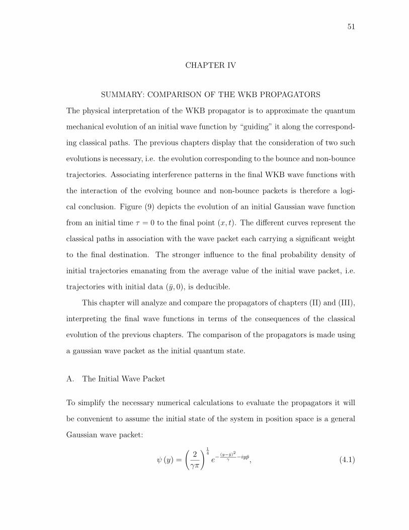
51

CHAPTER IV

SUMMARY: COMPARISON OF THE WKB PROPAGATORS

The physical interpretation of the WKB propagator is to approximate the quantum

mechanical evolution of an initial wave function by “guiding” it along the correspond-

ing classical paths. The previous chapters display that the consideration of two such

evolutions is necessary, i.e. the evolution corresponding to the bounce and non-bounce

trajectories. Associating interference patterns in the final WKB wave functions with

the interaction of the evolving bounce and non-bounce packets is therefore a logi-

cal conclusion. Figure (9) depicts the evolution of an initial Gaussian wave function

from an initial time τ = 0 to the final point (x, t). The different curves represent the

classical paths in association with the wave packet each carrying a significant weight

to the final destination. The stronger influence to the final probability density of

initial trajectories emanating from the average value of the initial wave packet, i.e.

trajectories with initial data (y, 0), is deducible.

This chapter will analyze and compare the propagators of chapters (II) and (III),

interpreting the final wave functions in terms of the consequences of the classical

evolution of the previous chapters. The comparison of the propagators is made using

a gaussian wave packet as the initial quantum state.

A. The Initial Wave Packet

To simplify the necessary numerical calculations to evaluate the propagators it will

be convenient to assume the initial state of the system in position space is a general

Gaussian wave packet:

ψ (y) =

(2

γπ

) 14

e−(y−y)2

γ−iyp, (4.1)

52

y�qHΤL

Τ

Hx,tL

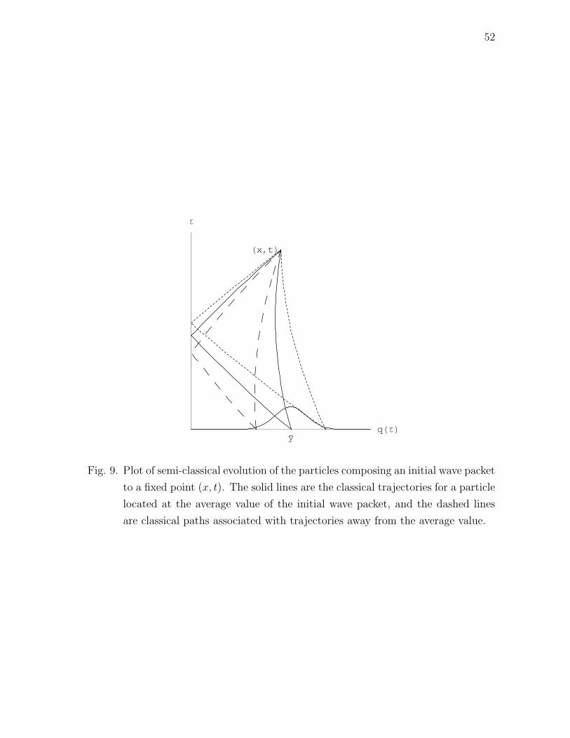
Fig. 9. Plot of semi-classical evolution of the particles composing an initial wave packet

to a fixed point (x, t). The solid lines are the classical trajectories for a particle

located at the average value of the initial wave packet, and the dashed lines

are classical paths associated with trajectories away from the average value.

53

where y denotes the initial position, the average initial position is y, and the average

initial momentum is p. The constant γ is associated with the width of the initial

wave packet. The initial wave packet in momentum space is the Fourier transform of

the initial position space wave packet:

φ (p) =(

γ

2π

) 14

e−γ(p+p)2

4−iy(p+p). (4.2)

The choice of the parameters for the wave packets should be chosen so that a negligible

amount of the position space wave packet extends into the forbidden region (y < 0).

B. The Propagators Constructed from Non-bounce Paths

From equations (2.84) and (3.52), the propagators constructed from non-bounce tra-

jectories are:

Uyd (x, y, t) =1√4πit

exp

[i

(2

3t3 + t2

[x− y

t− t

]+ t

(1

4

[x− y

t− t

]2

+ y

))]

Upd(x, p, t) =1√2π

exp

[i

(−t3

3+ t

(p2 + x

)− p

(t2 + pt− x

))],

and the final wave functions for the initial position and initial momentum formulations

are respectively:

Ψy(x, t) =∫ by

ay

dy ψ(y) Uyd(x, y, t)

=

(2

γπ

) 14 exp

[− y2

γ+ i

(x2

4t+ xt

2− t3

12

)]

√4πit

∫ by

ay

dy e−y2ωy+yλy

=

(2

γπ

) 14 exp

[− y2

γ+

λ2y

4ωy+ i

(x2

4t+ xt

2− t3

12

)]

√4πit

∫ by

ay

dy e−(

y√

ωy− λy2√

ωy

)2

(4.3)

Ψp(x, t) =∫ bp

ap

dp φ(p) Uyd(x, y, t)

=(

γ

8π3

) 14

exp

[− p2γ

4+ i

(xt− t3

3− py

)] ∫ bp

ap

dp e−p2ωp+λpp

54

=(

γ

8π3

) 14

exp

[− p2γ

4+

λ2p

4ωp

+ i

(xt− t3

3− py

)]

×∫ bp

ap

dp e−(

p√

ωp− λp2√

ωp

)2

. (4.4)

Here, the limits of integration are consistent with the classical limits given in tables

(I) and (II). The functions ω and λ are:

ωy =1

γ− i

4t(4.5)

λy =2y

γ+ i

(t

2− x

2t− p

)(4.6)

ωp =γ

4+ it (4.7)

λp = −γp

2+ i

(x− t2 − y

). (4.8)

Since the WKB propagators are equivalent to their exact Quantum Mechanical

counterparts, with the exception of the allowable limits of integration, the final wave

functions after propagation would be equivalent if not for the WKB limit constraints,

in other words the relationship between the WKB propagators in momentum and

position space is not the “complete” Fourier transform since the limits of integration

do not encompass all possible initial data but only those values which are classically

allowable, and the classically allowable regions are not equivalent for the two cases.

However, the advantage of using an initial Gaussian wave packet is that if the limits

lie outside the “effective” support, Cα, of the initial wave function (i.e. the domain of

initial data (position or momentum) such that the initial wave packet is comparable

to its maximum, located at y or p), then the extension of the limits in equations

(4.3) and (4.4) to ±∞ is permissible with negligible contribution from the classically

forbidden region.

Figure 10 gives a depiction of this behavior for the real parts of the final wave

functions. From tables (I) and (II) the classical limits on the initial momentum and

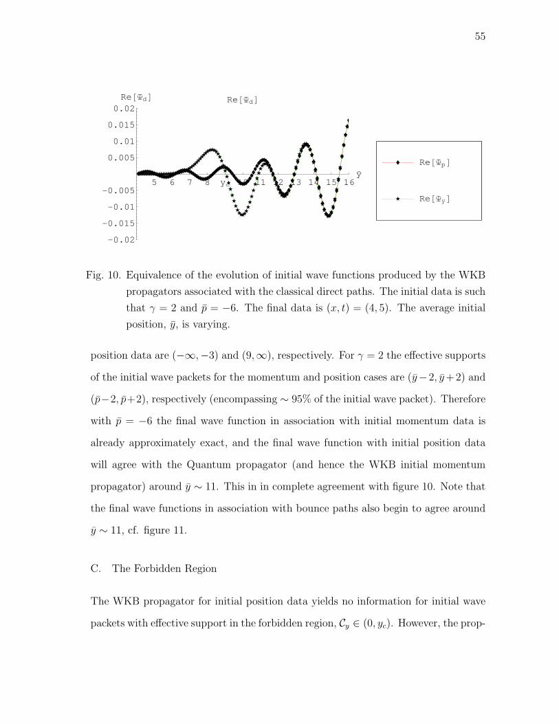
55

5 6 7 8 yc 10 11 12 13 14 15 16y�

-0.02

-0.015

-0.01

-0.005

0.005

0.01

0.015

0.02Re@YdD Re@YdD

Re@YyD

Re@YpD

Fig. 10. Equivalence of the evolution of initial wave functions produced by the WKB

propagators associated with the classical direct paths. The initial data is such

that γ = 2 and p = −6. The final data is (x, t) = (4, 5). The average initial

position, y, is varying.

position data are (−∞,−3) and (9,∞), respectively. For γ = 2 the effective supports

of the initial wave packets for the momentum and position cases are (y−2, y +2) and

(p−2, p+2), respectively (encompassing ∼ 95% of the initial wave packet). Therefore

with p = −6 the final wave function in association with initial momentum data is

already approximately exact, and the final wave function with initial position data

will agree with the Quantum propagator (and hence the WKB initial momentum

propagator) around y ∼ 11. This in in complete agreement with figure 10. Note that

the final wave functions in association with bounce paths also begin to agree around

y ∼ 11, cf. figure 11.

C. The Forbidden Region

The WKB propagator for initial position data yields no information for initial wave

packets with effective support in the forbidden region, Cy ∈ (0, yc). However, the prop-

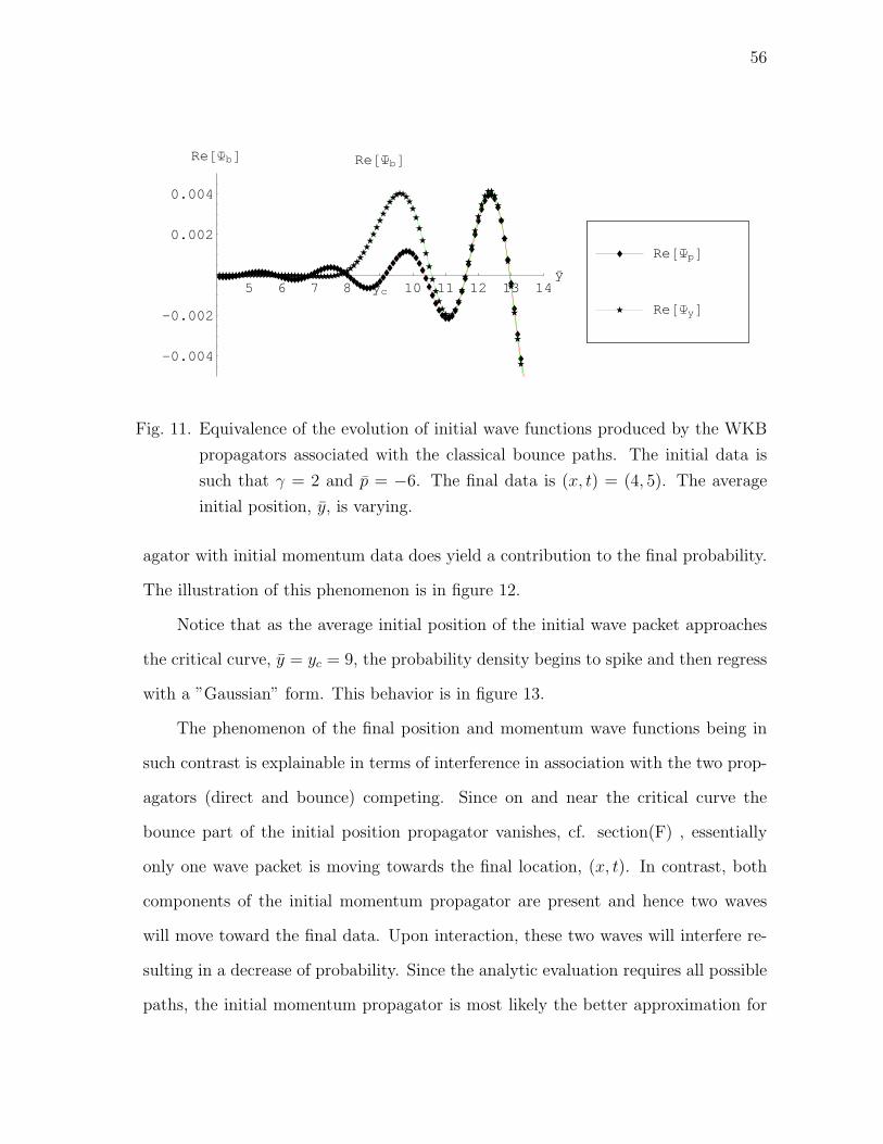
56

5 6 7 8 yc 10 11 12 13 14y�

-0.004

-0.002

0.002

0.004

Re@YbD Re@YbD

Re@YyD

Re@YpD

Fig. 11. Equivalence of the evolution of initial wave functions produced by the WKB

propagators associated with the classical bounce paths. The initial data is

such that γ = 2 and p = −6. The final data is (x, t) = (4, 5). The average

initial position, y, is varying.

agator with initial momentum data does yield a contribution to the final probability.

The illustration of this phenomenon is in figure 12.

Notice that as the average initial position of the initial wave packet approaches

the critical curve, y = yc = 9, the probability density begins to spike and then regress

with a ”Gaussian” form. This behavior is in figure 13.

The phenomenon of the final position and momentum wave functions being in

such contrast is explainable in terms of interference in association with the two prop-

agators (direct and bounce) competing. Since on and near the critical curve the

bounce part of the initial position propagator vanishes, cf. section(F) , essentially

only one wave packet is moving towards the final location, (x, t). In contrast, both

components of the initial momentum propagator are present and hence two waves

will move toward the final data. Upon interaction, these two waves will interfere re-

sulting in a decrease of probability. Since the analytic evaluation requires all possible

paths, the initial momentum propagator is most likely the better approximation for

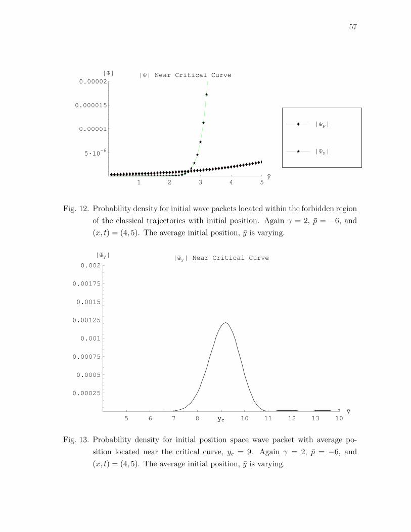
57

1 2 3 4 5y�

5·10-6

0.00001

0.000015

0.00002ÈYÈ ÈYÈ Near Critical Curve

ÈYyÈ

ÈYpÈ

Fig. 12. Probability density for initial wave packets located within the forbidden region

of the classical trajectories with initial position. Again γ = 2, p = −6, and

(x, t) = (4, 5). The average initial position, y is varying.

5 6 7 8 yc 10 11 12 13yc 10y�

0.00025

0.0005

0.00075

0.001

0.00125

0.0015

0.00175

0.002

ÈYyÈ ÈYyÈ Near Critical Curve

Fig. 13. Probability density for initial position space wave packet with average po-

sition located near the critical curve, yc = 9. Again γ = 2, p = −6, and

(x, t) = (4, 5). The average initial position, y is varying.

58

the scenario.

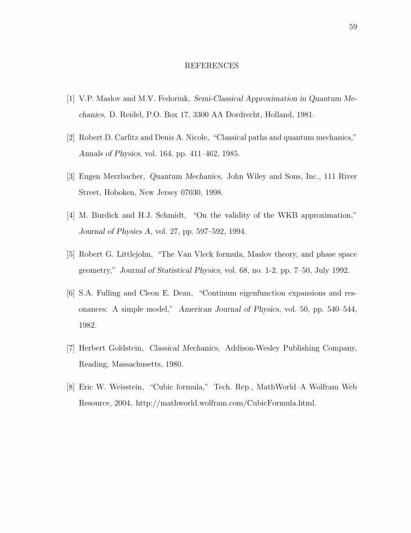
59

REFERENCES

[1] V.P. Maslov and M.V. Fedoriuk, Semi-Classical Approximation in Quantum Me-

chanics, D. Reidel, P.O. Box 17, 3300 AA Dordrecht, Holland, 1981.

[2] Robert D. Carlitz and Denis A. Nicole, “Classical paths and quantum mechanics,”

Annals of Physics, vol. 164, pp. 411–462, 1985.

[3] Eugen Merzbacher, Quantum Mechanics, John Wiley and Sons, Inc., 111 River

Street, Hoboken, New Jersey 07030, 1998.

[4] M. Burdick and H.J. Schmidt, “On the validity of the WKB approximation,”

Journal of Physics A, vol. 27, pp. 597–592, 1994.

[5] Robert G. Littlejohn, “The Van Vleck formula, Maslov theory, and phase space

geometry,” Journal of Statistical Physics, vol. 68, no. 1-2, pp. 7–50, July 1992.

[6] S.A. Fulling and Cleon E. Dean, “Continum eigenfunction expansions and res-

onances: A simple model,” American Journal of Physics, vol. 50, pp. 540–544,

1982.

[7] Herbert Goldstein, Classical Mechanics, Addison-Wesley Publishing Company,

Reading, Massachusetts, 1980.

[8] Eric W. Weisstein, “Cubic formula,” Tech. Rep., MathWorld–A Wolfram Web

Resource, 2004, http://mathworld.wolfram.com/CubicFormula.html.

60

VITA

Todd Austin Zapata received his B.S. in Nuclear Engineering from Texas A&M

University in 2005. He is currently a graduate student at Texas A&M University. His

email address is tazapata@neo.tamu.edu . Todd Austin Zapata resides at 409 Tauber

St., College Station, TX 77840.

The typist for this thesis was Todd Austin Zapata.