Embed Size (px)
Citation preview
IZA DP No. 3943
The Wooldridge Method for the Initial ValuesProblem Is Simple: What About Performance?
Alpaslan Akay
DI
SC
US
SI
ON
PA
PE
R S
ER
IE
S
Forschungsinstitutzur Zukunft der ArbeitInstitute for the Studyof Labor
January 2009
The Wooldridge Method for the
Initial Values Problem Is Simple: What About Performance?
Alpaslan Akay IZA
Discussion Paper No. 3943 January 2009
IZA
P.O. Box 7240 53072 Bonn
Germany
Phone: +49-228-3894-0 Fax: +49-228-3894-180
E-mail: [email protected]
Any opinions expressed here are those of the author(s) and not those of IZA. Research published in this series may include views on policy, but the institute itself takes no institutional policy positions. The Institute for the Study of Labor (IZA) in Bonn is a local and virtual international research center and a place of communication between science, politics and business. IZA is an independent nonprofit organization supported by Deutsche Post World Net. The center is associated with the University of Bonn and offers a stimulating research environment through its international network, workshops and conferences, data service, project support, research visits and doctoral program. IZA engages in (i) original and internationally competitive research in all fields of labor economics, (ii) development of policy concepts, and (iii) dissemination of research results and concepts to the interested public. IZA Discussion Papers often represent preliminary work and are circulated to encourage discussion. Citation of such a paper should account for its provisional character. A revised version may be available directly from the author.

IZA Discussion Paper No. 3943 January 2009
ABSTRACT
The Wooldridge Method for the Initial Values Problem Is Simple: What About Performance?*
The Wooldridge method is based on a simple and novel strategy to deal with the initial values problem in the nonlinear dynamic random-effects panel data models. This characteristic of the method makes it very attractive in empirical applications. However, its finite sample performance is not known as of yet. In this paper we investigate the performance of this method in comparison with an ideal case in which the initial values are known constants, the worst scenario based on exogenous initial values assumption, and the Heckman’s reduced-form approximation method which is widely used in the literature. The dynamic random-effects probit and tobit (type1) models are used as the working examples. Various designs of Monte Carlo Experiments with balanced and unbalanced panel data sets, and also two full length empirical applications are provided. The results suggest that the Wooldridge method works very well for the panels with moderately long durations (longer than 5-8 periods). In short panels Heckman’s reduced-form approximation is suggested (shorter than 5 periods). It is also found that all methods perform equally well for panels of long durations (longer than 10-15 periods). JEL Classification: C23, C25 Keywords: initial values problem, dynamic probit and tobit models, Monte Carlo
experiment, Heckman’s reduced-form approximation, Wooldridge method Corresponding author: Alpaslan Akay IZA P.O. Box 7240 53072 Bonn Germany E-mail: [email protected]
* I thank Steven Bond, Lennart Flood, Konstantinos Tatsiramos, Arne Uhlendorff, Måns Söderbom, Roger Wahlberg, Elias Tsakas, Peter Martinsson, Melanie Khamis and seminar participants at Gothenburg University for their valuable comments.
1 Introduction
One of the crucial issues in the estimation of a dynamic panel data random-e¤ects
models is the initial values problem (Blundell and Smith, 1991; Arellano and Bover,
1997; Blundell and Bond, 1998; Arellano and Honore, 2001; Honore, 2002; Arel-
lano and Carrasco, 2003; De Jong and Herrera, 2005; Arellano and Hahn, 2005;
Wooldridge, 2005; Honore and Tamer, 2006). This problem occurs when the history
of a stochastic process is not observed from the very beginning. Almost all panel data
sets used in microeconometric practice today contain information about individuals
entered into the process before the observation period. Ad hoc treatments of this
problem are prone to bias and inconsistent estimators as well as a wrong inference of
the magnitude of true (structural) and spurious state dependence (Heckman, 1981;
Honore, 2002; Hsiao, 2003; Honore and Tamer, 2006).
This problem is either ignored by assuming that the initial values have not been
in e¤ect with what happened in the unknown past, i.e. exogenous variables, inde-
pendent from the exogenous variables and the unobserved individual-e¤ects (het-
erogeneity), or the stochastic process underlying the model is assumed as is in the
steady state (Heckman, 1981; Card and Sullivan, 1988). The exogenous initial values
assumption is very naive and may lead to severe bias if the initial observations have
been created with the evolution of observed and unobserved characteristics in the
past. The initial stationary assumption is also very unattractive especially when
age-trended variables drive the process (Heckman, 1981, Hsiao, 2003).
A realistic solution strategy is �rst suggested by Heckman (1981) which consid-
ers the initial values are endogenous variables with a probability distribution condi-
3

tioned on the exogenous variables and unobserved individual-e¤ects. The strategy
of the method is to approximate the conditional probability of initial values with
reduced-form equations using available pre-sample information. This leads to very
�exible functional forms. Using a small scale Monte Carlo study, Heckman (1981)
shows that this solution method performs very well. The main problem of this
method in practice is that the approximation of the conditional probability of initial
values leads to a simultaneous estimation problem of the reduced-form and structural
model which can create a large computational burden in the estimation process.
One other way to ensure that initial values are not a problem in the estima-
tion is to use a �xed-e¤ects approach. The conditional distribution of unobserved
individual-e¤ects does not play a role in the estimation process of this approach.
However, the �xed-e¤ects approach can be seriously biased as it su¤ers from so-
called incidental parameters problem (Neyman and Scott, 1948). Alternatively, some
of the recently developed nonparametric methods can be used (Honore and Kyriazi-
dou, 2000; Hu, 2002; Honore, 2003). For instance, Honore and Kyriazidou (2000)
provide a �xed-e¤ects logit model based on kernel-weighted GMM estimators which
also absorb the initial values problem. These estimators though have some problems.
For instance, it is not possible to calculate average partial e¤ects (Wooldridge, 2005).
Thus, the random-e¤ects speci�cation is still attractive in practice and a solution
for the initial values problem is inevitable.
Wooldridge (2005) has recently provided a very simple alternative to the Heck-
man�s reduced-form approximation to solve the initial values problem. This method
leads to very simple and tractable likelihoods that is not di¤erent than standard sta-
4

tic random-e¤ects model. It is based on an auxiliary distribution of the unobserved
individual-e¤ects which is conditioned on the initial values and exogenous variables.
It is also very useful in random-e¤ects speci�cations as it is very similar to Cham-
berlain approach (1984) with which one can also deal with the possible correlation
between exogenous variables and unobserved individual-e¤ects. To our knowledge,
although there is a growing literature which routinely uses this method in empiri-
cal applications (Contayannis et al., 2004), there is no rigorous study on the �nite
sample performance of the method as an alternative to Heckman�s reduced-form
approximation.
The main aim of this paper is to provide Monte Carlo Experiments (MCE)
and present real data evidence to investigate the �nite sample performance of the
Wooldridge method. The dynamic panel data random-e¤ects probit and tobit (type
I) models are used as working examples. The paper also aims to compare the
performance of the Wooldridge method with the results produced by the exogenous
initial values assumption and the Heckman�s reduced-form approximation. First,
we conduct various designs of MCE with balanced panel data sets. However, as
explained in Honore (2002), ad hoc treatments of the initial values problem are
especially unappealing with unbalanced panel data sets. This is generally the case
in the empirical applications and thus, various designs of MCE with unbalanced
panel data sets are also presented. The real microeconomic panel data sets contain
more complicated structure compared to any MCE design. The paper also gives
two full scale real data applications which concentrate on intertemporal labor force
participation and hours of work decisions of married women in Sweden between 1992
5

and 2001.
Given that the aim of estimating a dynamic panel data models is to identify the
di¤erent sources of persistence, the initial values problem plays a very important
role. The result suggests that misspeci�cation of the conditional distribution of the
initial values leads to a serious bias on both persistence which is due to structural or
spurious reasons. The exogenous initial values assumption, for instance, would lead
to overestimation of the true and underestimation of the spurious state dependence.
We �nd that the Wooldridge method works very well but it is not as successful
as Heckman�s reduced-form approximation for very short panels (shorter than 5).
The Wooldridge method gives almost the same results with the Heckman�s method
for moderately long panels (longer than 5 � 8 periods). One of the other and very
intuitive result is that the performance of all methods tends to be equal for the
panels of very long durations (longer than 10� 15 periods).
The paper is organized as follows: the next section will summarize the mod-
els and estimation strategies with di¤erent solution methods of the initial values
problem. Section 3 presents our MCE designs and the results. Section 4 gives
two empirical applications to the intertemporal labour force participation and hours
of work decisions of married women in Sweden between 1992 and 2001. Section 5
concludes.
6
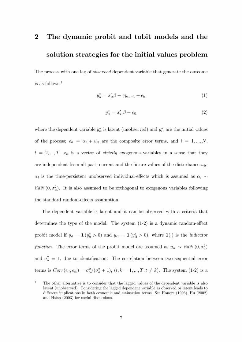
2 The dynamic probit and tobit models and the
solution strategies for the initial values problem
The process with one lag of observed dependent variable that generate the outcome
is as follows.1
y�it = x0it� + yi;t�1 + �it (1)
y�i1 = x0i1� + �i1 (2)
where the dependent variable y�it is latent (unobserved) and y�i1 are the initial values
of the process; �it = �i + uit are the composite error terms, and i = 1; :::; N ,
t = 2; :::; T ; xit is a vector of strictly exogenous variables in a sense that they
are independent from all past, current and the future values of the disturbance uit;
�i is the time-persistent unobserved individual-e¤ects which is assumed as �i �
iidN (0; �2�). It is also assumed to be orthogonal to exogenous variables following
the standard random-e¤ects assumption.
The dependent variable is latent and it can be observed with a criteria that
determines the type of the model. The system (1-2) is a dynamic random-e¤ect
probit model if yit = 1 (y�it > 0) and yi1 = 1 (y�i1 > 0), where 1(:) is the indicator
function. The error terms of the probit model are assumed as uit � iidN (0; �2u)
and �2u = 1, due to identi�cation. The correlation between two sequential error
terms is Corr(�it; �ik) = �2�=(�2� + 1), (t; k = 1; :::; T ; t 6= k). The system (1-2) is a
1 The other alternative is to consider that the lagged values of the dependent variable is alsolatent (unobserved). Considering the lagged dependent variable as observed or latent leads todi¤erent implications in both economic and estimation terms. See Honore (1993), Hu (2002)and Hsiao (2003) for useful discussions.
7
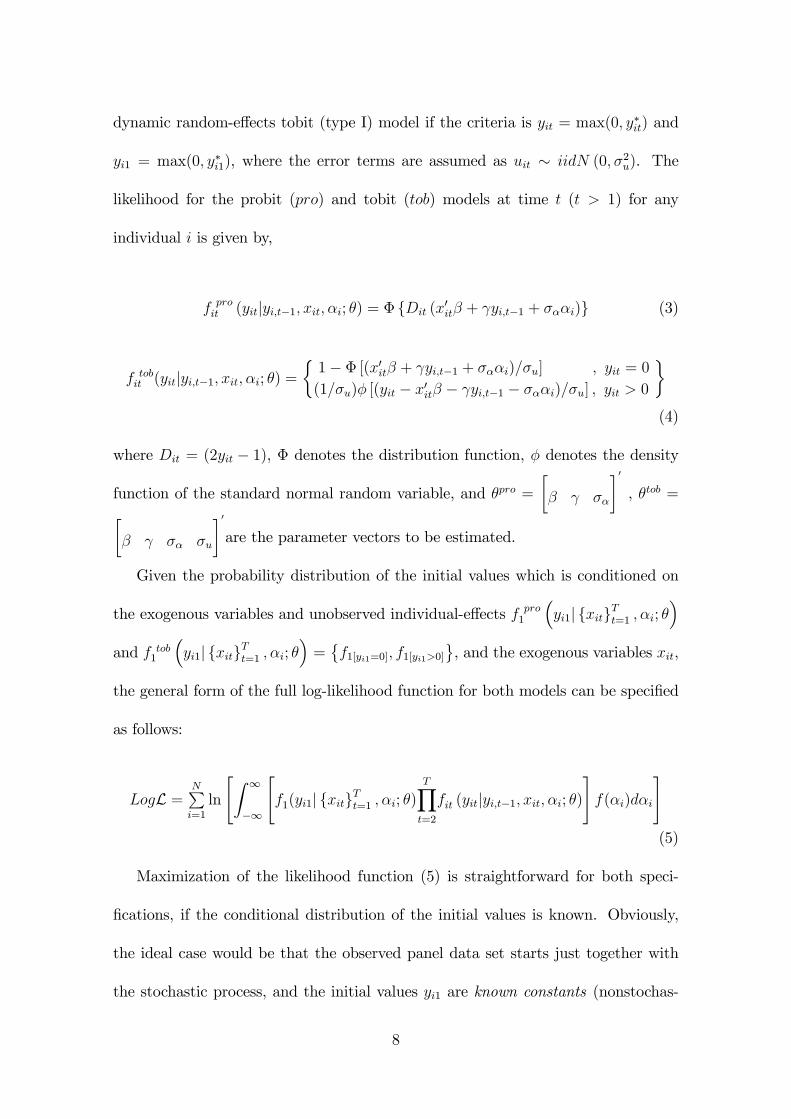
dynamic random-e¤ects tobit (type I) model if the criteria is yit = max(0; y�it) and
yi1 = max(0; y�i1), where the error terms are assumed as uit � iidN (0; �2u). The
likelihood for the probit (pro) and tobit (tob) models at time t (t > 1) for any
individual i is given by,
f proit (yitjyi;t�1; xit; �i; �) = � fDit (x
0it� + yi;t�1 + ���i)g (3)
f tobit (yitjyi;t�1; xit; �i; �) =
�1� � [(x0it� + yi;t�1 + ���i)=�u] ; yit = 0
(1=�u)� [(yit � x0it� � yi;t�1 � ���i)=�u] ; yit > 0
�(4)
where Dit = (2yit � 1), � denotes the distribution function, � denotes the density
function of the standard normal random variable, and �pro =�� ��
�0, �tob =�
� �� �u
�0are the parameter vectors to be estimated.
Given the probability distribution of the initial values which is conditioned on
the exogenous variables and unobserved individual-e¤ects f pro1
�yi1j fxitgTt=1 ; �i; �
�and f tob
1
�yi1j fxitgTt=1 ; �i; �
�=�f1[yi1=0]; f1[yi1>0]
, and the exogenous variables xit,
the general form of the full log-likelihood function for both models can be speci�ed
as follows:
LogL =NPi=1
ln
"Z 1
�1
"f1(yi1j fxitg
Tt=1 ; �i; �)
TYt=2
fit (yitjyi;t�1; xit; �i; �)#f(�i)d�i
#(5)
Maximization of the likelihood function (5) is straightforward for both speci-
�cations, if the conditional distribution of the initial values is known. Obviously,
the ideal case would be that the observed panel data set starts just together with
the stochastic process, and the initial values yi1 are known constants (nonstochas-
8
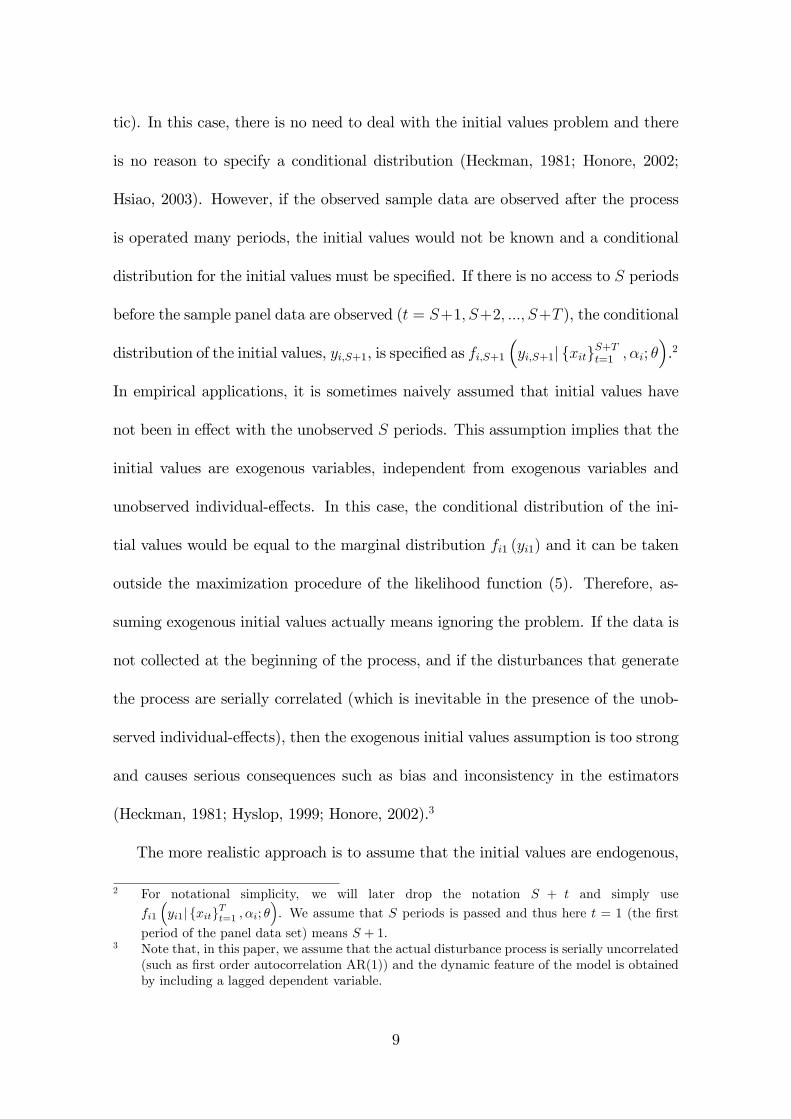
tic). In this case, there is no need to deal with the initial values problem and there
is no reason to specify a conditional distribution (Heckman, 1981; Honore, 2002;
Hsiao, 2003). However, if the observed sample data are observed after the process
is operated many periods, the initial values would not be known and a conditional
distribution for the initial values must be speci�ed. If there is no access to S periods
before the sample panel data are observed (t = S+1; S+2; :::; S+T ), the conditional
distribution of the initial values, yi;S+1, is speci�ed as fi;S+1�yi;S+1j fxitgS+Tt=1 ; �i; �
�.2
In empirical applications, it is sometimes naively assumed that initial values have
not been in e¤ect with the unobserved S periods. This assumption implies that the
initial values are exogenous variables, independent from exogenous variables and
unobserved individual-e¤ects. In this case, the conditional distribution of the ini-
tial values would be equal to the marginal distribution fi1 (yi1) and it can be taken
outside the maximization procedure of the likelihood function (5). Therefore, as-
suming exogenous initial values actually means ignoring the problem. If the data is
not collected at the beginning of the process, and if the disturbances that generate
the process are serially correlated (which is inevitable in the presence of the unob-
served individual-e¤ects), then the exogenous initial values assumption is too strong
and causes serious consequences such as bias and inconsistency in the estimators
(Heckman, 1981; Hyslop, 1999; Honore, 2002).3
The more realistic approach is to assume that the initial values are endogenous,
2 For notational simplicity, we will later drop the notation S + t and simply use
fi1
�yi1j fxitgTt=1 ; �i; �
�. We assume that S periods is passed and thus here t = 1 (the �rst
period of the panel data set) means S + 1:3 Note that, in this paper, we assume that the actual disturbance process is serially uncorrelated
(such as �rst order autocorrelation AR(1)) and the dynamic feature of the model is obtainedby including a lagged dependent variable.
9
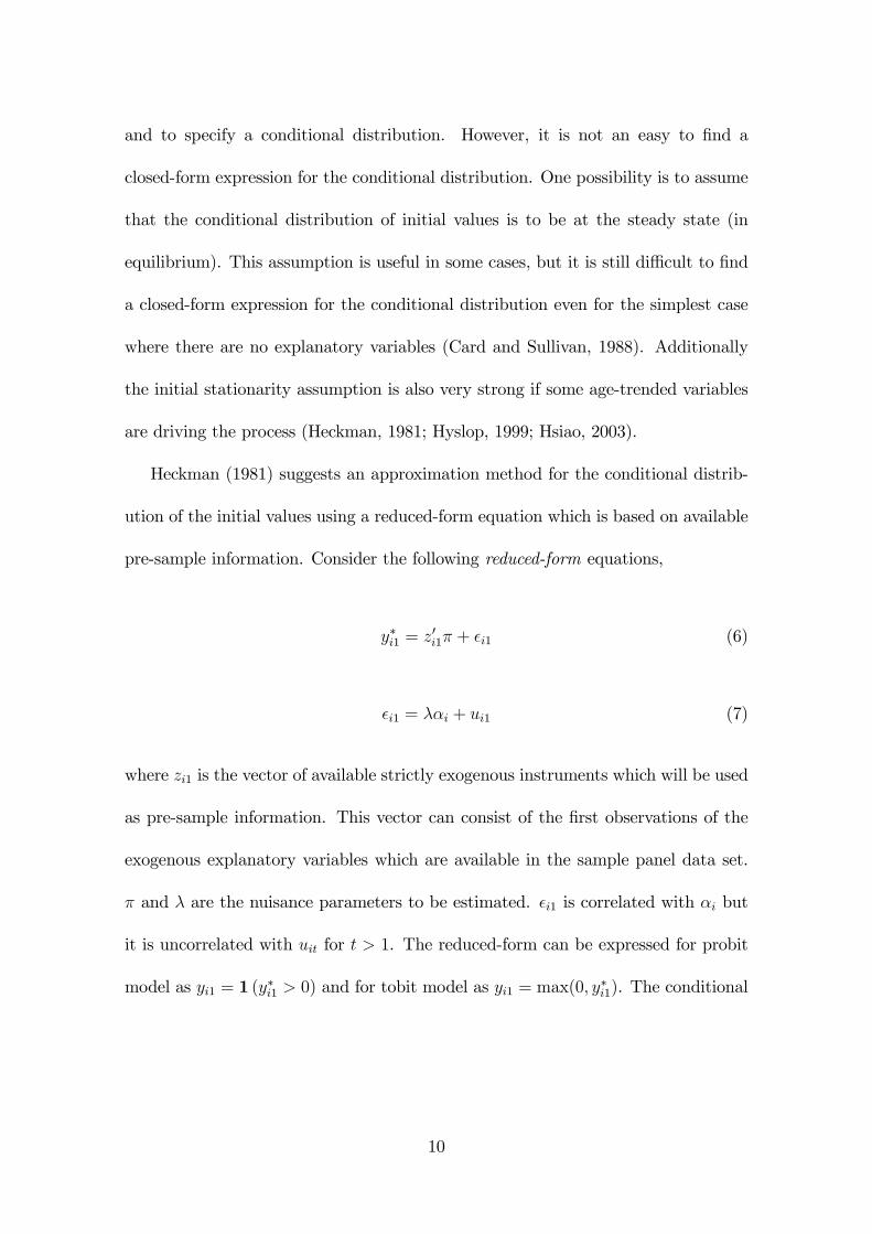
and to specify a conditional distribution. However, it is not an easy to �nd a
closed-form expression for the conditional distribution. One possibility is to assume
that the conditional distribution of initial values is to be at the steady state (in
equilibrium). This assumption is useful in some cases, but it is still di¢ cult to �nd
a closed-form expression for the conditional distribution even for the simplest case
where there are no explanatory variables (Card and Sullivan, 1988). Additionally
the initial stationarity assumption is also very strong if some age-trended variables
are driving the process (Heckman, 1981; Hyslop, 1999; Hsiao, 2003).
Heckman (1981) suggests an approximation method for the conditional distrib-
ution of the initial values using a reduced-form equation which is based on available
pre-sample information. Consider the following reduced-form equations,
y�i1 = z0i1� + �i1 (6)
�i1 = ��i + ui1 (7)
where zi1 is the vector of available strictly exogenous instruments which will be used
as pre-sample information. This vector can consist of the �rst observations of the
exogenous explanatory variables which are available in the sample panel data set.
� and � are the nuisance parameters to be estimated. �i1 is correlated with �i but
it is uncorrelated with uit for t > 1. The reduced-form can be expressed for probit
model as yi1 = 1 (y�i1 > 0) and for tobit model as yi1 = max(0; y�i1). The conditional
10
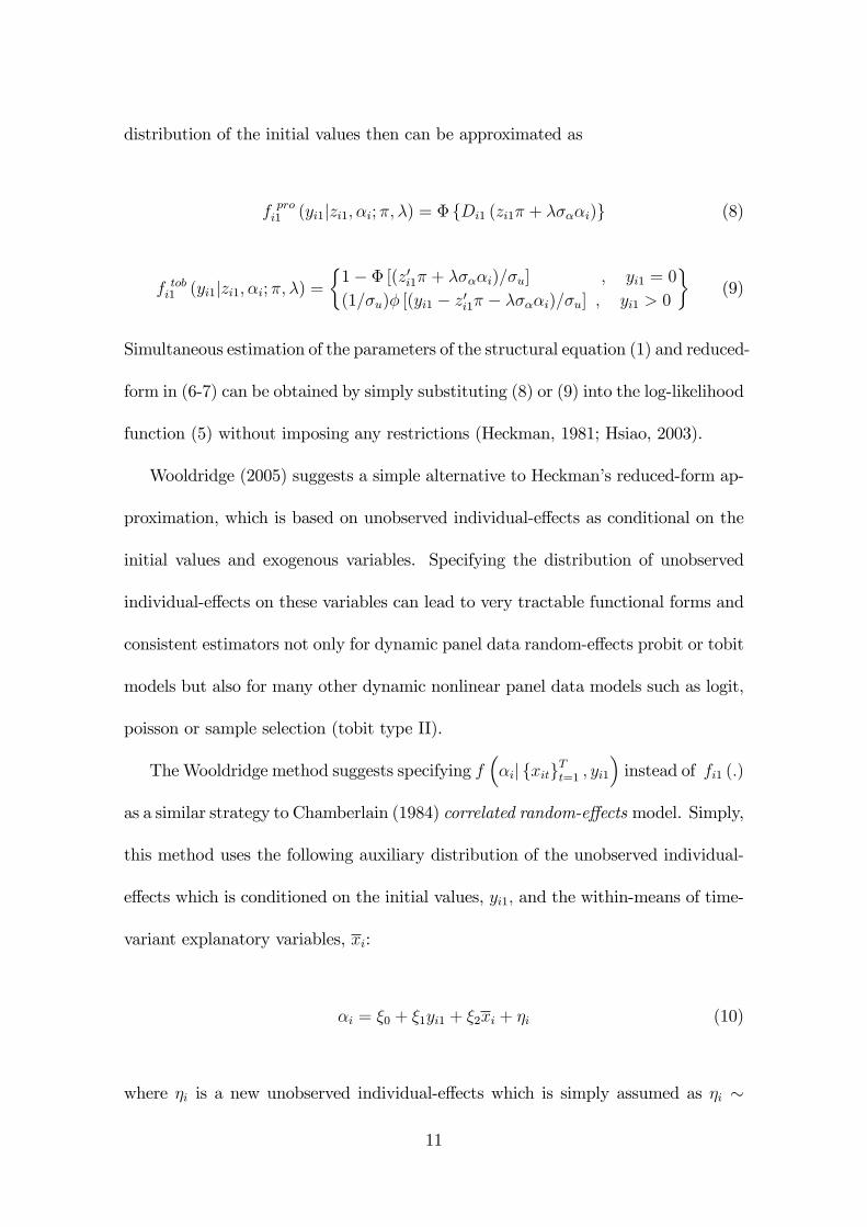
distribution of the initial values then can be approximated as
f proi1 (yi1jzi1; �i; �; �) = � fDi1 (zi1� + ����i)g (8)
f tobi1 (yi1jzi1; �i; �; �) =
�1� � [(z0i1� + ����i)=�u] ; yi1 = 0
(1=�u)� [(yi1 � z0i1� � ����i)=�u] ; yi1 > 0
�(9)
Simultaneous estimation of the parameters of the structural equation (1) and reduced-
form in (6-7) can be obtained by simply substituting (8) or (9) into the log-likelihood
function (5) without imposing any restrictions (Heckman, 1981; Hsiao, 2003).
Wooldridge (2005) suggests a simple alternative to Heckman�s reduced-form ap-
proximation, which is based on unobserved individual-e¤ects as conditional on the
initial values and exogenous variables. Specifying the distribution of unobserved
individual-e¤ects on these variables can lead to very tractable functional forms and
consistent estimators not only for dynamic panel data random-e¤ects probit or tobit
models but also for many other dynamic nonlinear panel data models such as logit,
poisson or sample selection (tobit type II).
TheWooldridge method suggests specifying f��ij fxitgTt=1 ; yi1
�instead of fi1 (:)
as a similar strategy to Chamberlain (1984) correlated random-e¤ects model. Simply,
this method uses the following auxiliary distribution of the unobserved individual-
e¤ects which is conditioned on the initial values, yi1; and the within-means of time-
variant explanatory variables, xi:
�i = �0 + �1yi1 + �2xi + �i (10)
where �i is a new unobserved individual-e¤ects which is simply assumed as �i �
11

iidN�0; �2�
�; �ijxi; yi1 � N
��0 + �1yi1 + �2xi; �
2�
�; and xi = 1
T
XT
t=1xit.4 Thus, we
obtain a conditional likelihood which is based on the joint distribution of obser-
vations conditional on initial values. The resulting likelihood function will be like
those in standard static random-e¤ect probit and tobit models. The parameters
can be easily estimated by using a standard random-e¤ects command in available
softwares.
The likelihood functions of probit and tobit models (5) involve only a single inte-
gral, which can be e¤ectively implemented by using Gaussian-Hermite Quadrature
and this tool will be employed in the maximization of likelihood functions in this
paper (Butler and Mo¢ tt, 1982). This method is less time consuming and more e¢ -
cient in comparison with the other alternative based on Monte Carlo integration with
a proper simulator (Gourieroux and Monfort, 1993; Hajivassiliou and Ruud,1994).
The details of the Gaussian-Hermite Quadrature applied in the paper is provided in
the Appendix together with the likelihood functions used in the estimation process.
3 Monte Carlo Experiments
Various designs of MCE are carried out with balanced and unbalanced panel data
sets to analyze the �nite sample performance of the Wooldridge method in compari-
son with; i) the ideal case, known initial values; ii) the worst case, exogenous initial
values assumption; and iii) Heckman�s reduced-form approximation. Our MCE (as
all calculations in this paper) is designed in Compaq Visual Fortran, and the op-
4 Note that we present the auxiliary conditional distribution of �i with a constant �0: Thus,the constant in the structural equation should be dropped.
12
timization for the likelihood functions is performed using ZXMIN , which is very
fast and robust optimization routine.5
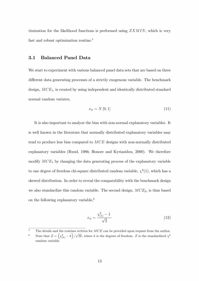
3.1 Balanced Panel Data
We start to experiment with various balanced panel data sets that are based on three
di¤erent data generating processes of a strictly exogenous variable. The benchmark
design,MCE1, is created by using independent and identically distributed standard
normal random variates,
xit � N [0; 1] (11)
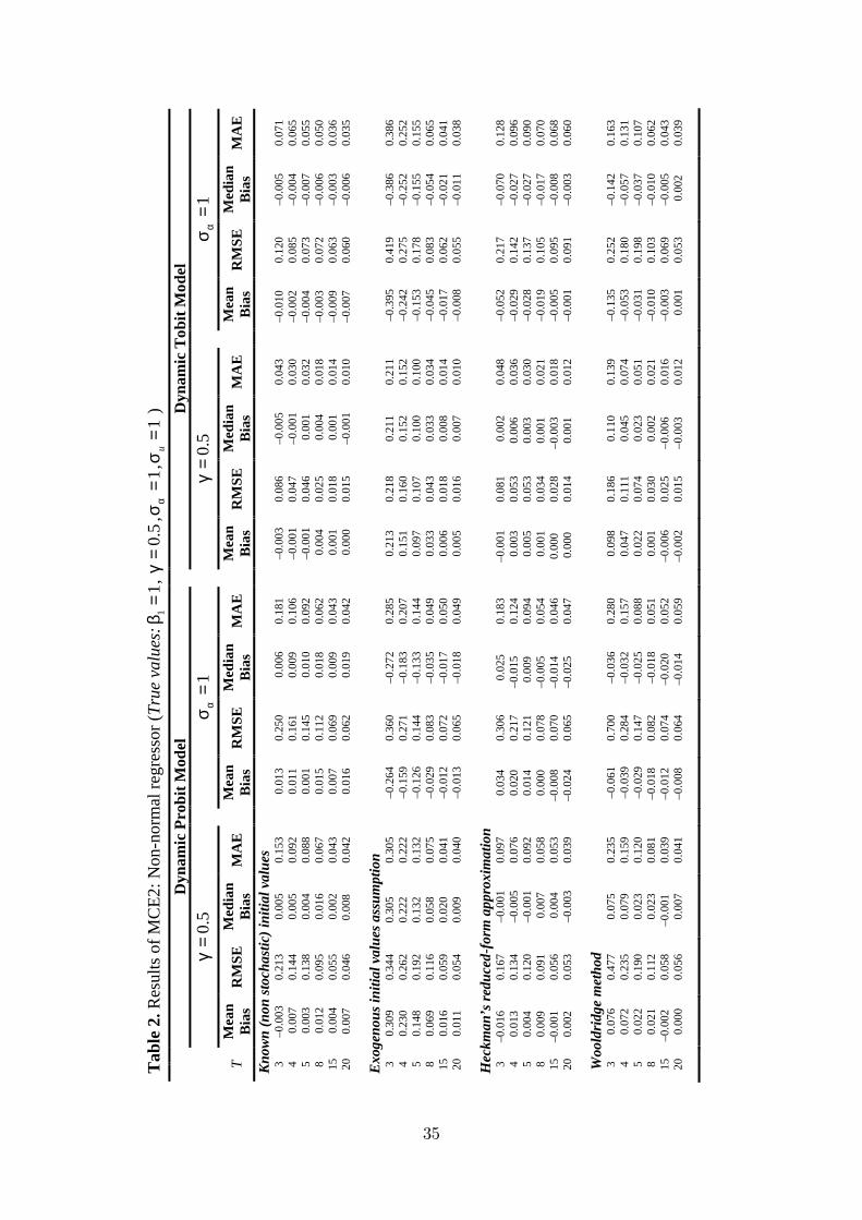
It is also important to analyze the bias with non-normal explanatory variables. It
is well known in the literature that normally distributed explanatory variables may
tend to produce less bias compared to MCE designs with non-normally distributed
explanatory variables (Ruud, 1986; Honore and Kyriazidou, 2000). We therefore
modify MCE1 by changing the data generating process of the explanatory variable
to one degree of freedom chi-square distributed random variable, �2(1); which has a
skewed distribution. In order to reveal the comparability with the benchmark design
we also standardize this random variable. The second design, MCE2, is thus based
on the following explanatory variable,6
xit ��2(1) � 1p
2(12)
5 The details and the routines written forMCE can be provided upon request from the author.6 Note that Z =
��2(k) � k
�=p2k, where k is the degrees of freedom. Z is the standardized �2
random variable.
13
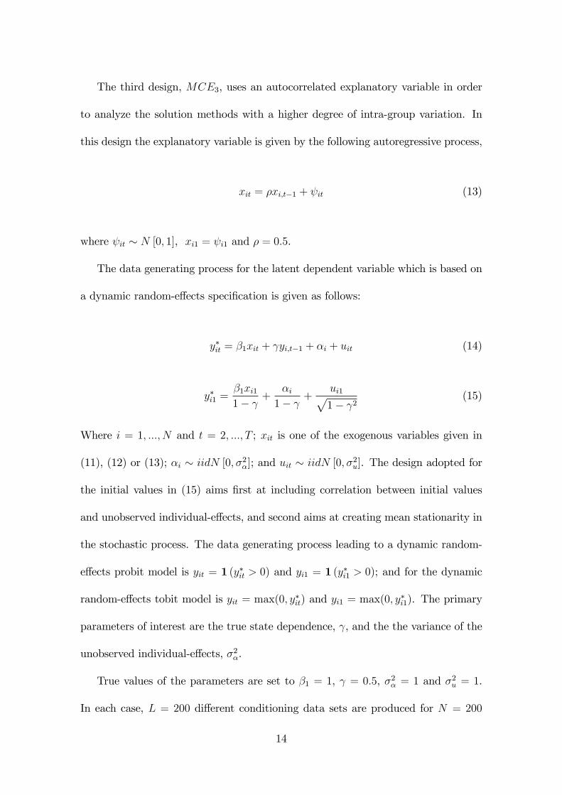
The third design, MCE3, uses an autocorrelated explanatory variable in order
to analyze the solution methods with a higher degree of intra-group variation. In
this design the explanatory variable is given by the following autoregressive process,
xit = �xi;t�1 + it (13)
where it � N [0; 1], xi1 = i1 and � = 0:5.
The data generating process for the latent dependent variable which is based on
a dynamic random-e¤ects speci�cation is given as follows:
y�it = �1xit + yi;t�1 + �i + uit (14)
y�i1 =�1xi11�
+�i1�
+ui1p1� 2
(15)
Where i = 1; :::; N and t = 2; :::; T ; xit is one of the exogenous variables given in
(11), (12) or (13); �i � iidN [0; �2�]; and uit � iidN [0; �2u]. The design adopted for
the initial values in (15) aims �rst at including correlation between initial values
and unobserved individual-e¤ects, and second aims at creating mean stationarity in
the stochastic process. The data generating process leading to a dynamic random-
e¤ects probit model is yit = 1 (y�it > 0) and yi1 = 1 (y�i1 > 0); and for the dynamic
random-e¤ects tobit model is yit = max(0; y�it) and yi1 = max(0; y�i1). The primary
parameters of interest are the true state dependence, , and the the variance of the
unobserved individual-e¤ects, �2�.
True values of the parameters are set to �1 = 1, = 0:5, �2� = 1 and �2u = 1.
In each case, L = 200 di¤erent conditioning data sets are produced for N = 200
14
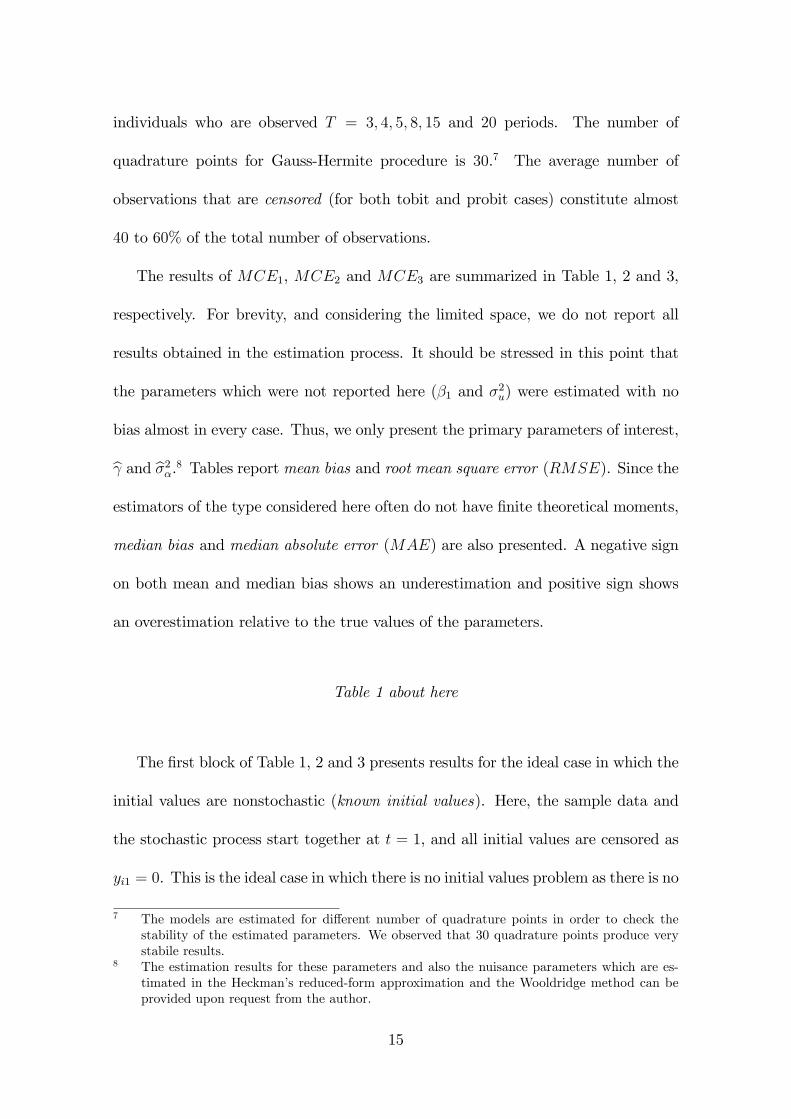
individuals who are observed T = 3; 4; 5; 8; 15 and 20 periods. The number of
quadrature points for Gauss-Hermite procedure is 30.7 The average number of
observations that are censored (for both tobit and probit cases) constitute almost
40 to 60% of the total number of observations.
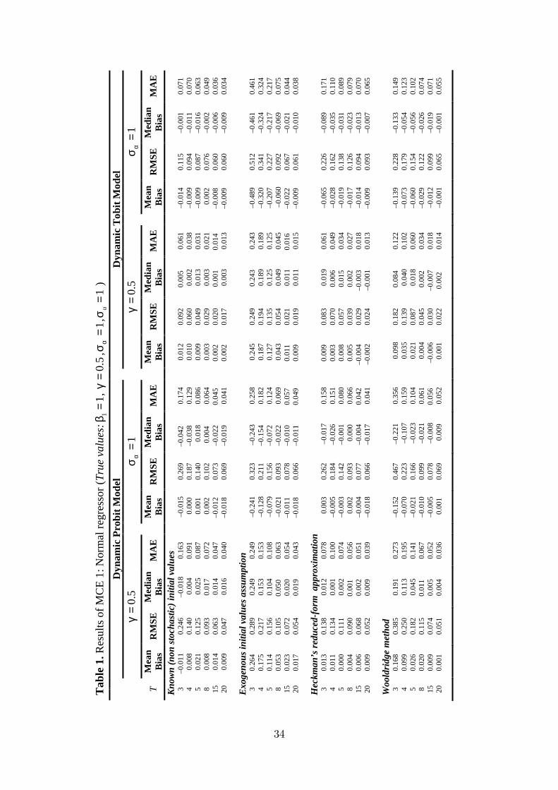
The results of MCE1, MCE2 and MCE3 are summarized in Table 1, 2 and 3,
respectively. For brevity, and considering the limited space, we do not report all
results obtained in the estimation process. It should be stressed in this point that
the parameters which were not reported here (�1 and �2u) were estimated with no
bias almost in every case. Thus, we only present the primary parameters of interest,
b and b�2�.8 Tables report mean bias and root mean square error (RMSE). Since the
estimators of the type considered here often do not have �nite theoretical moments,
median bias and median absolute error (MAE) are also presented. A negative sign
on both mean and median bias shows an underestimation and positive sign shows
an overestimation relative to the true values of the parameters.
Table 1 about here
The �rst block of Table 1, 2 and 3 presents results for the ideal case in which the
initial values are nonstochastic (known initial values). Here, the sample data and
the stochastic process start together at t = 1, and all initial values are censored as
yi1 = 0. This is the ideal case in which there is no initial values problem as there is no
7 The models are estimated for di¤erent number of quadrature points in order to check thestability of the estimated parameters. We observed that 30 quadrature points produce verystabile results.
8 The estimation results for these parameters and also the nuisance parameters which are es-timated in the Heckman�s reduced-form approximation and the Wooldridge method can beprovided upon request from the author.
15
correlation between initial values and unobserved individual-e¤ects. Therefore, we
do not expect any positive or negative bias. In line with the expectations, almost no
bias is observed both for the true state dependence and the variance of unobserved
individual-e¤ects. The mean and median bias are very close to each other implying
that the bias has a symmetric distribution with a decreasing variance as the duration
of the panel data set is increased.
In order to create an initial values problem we operate the system S = 25
periods before the sample data are observed for T = 3; 4; 5; 8; 15 and 20. This means
that initial sample values (i.e. S = 26) have been created with the evolution of
the relationship between unobserved individual-e¤ects and the explanatory variable
during past 25 periods. The second block in Table 1, 2 and 3 presents the results
for the worst scenario which is based on the exogenous initial values assumption. In
our case, this assumption is clearly wrong and also very strong, and thus we expect
a sizeable bias on the estimated parameters. The assumption leads to a serious bias
for both parameters (see footnote 7). The true state dependence, , is seriously
overestimated while the variance of the e¤ect, �2�, is seriously underestimated. The
bias is 30 to 60% when T = 3, but it is gradually getting smaller as the duration of
the panel is increased, and there is almost no bias when the panel is longer than 15
periods. It is also observed that the result obtained in MCE1, MCE2 and MCE3
are very close to each other. The methods have not produced bigger bias for non-
normal and autocorrelated explanatory variables and even the bias is smaller for
some cases.
Third blocks in the tables present the results for the Heckman�s reduced-form
16
approximation. This method performs very well for all durations of the panels. The
bias is very small even with the smallest duration (T = 3) one can use with dynamic
panel data models (the bias is about 0 to 7%). The results for the Wooldridge
method are presented in the last block of the each table. This method performs
almost equally well with the Heckman�s reduced-form approximation. The main
di¤erence between these two methods occurs for the panels of very short durations
(T = 3 and 4). Similar to the exogenous initial values assumption, the Wooldridge
method also tends to produce overestimated true state dependence and underes-
timated variance of the unobserved individual-e¤ects for the short panels but the
bias is much smaller (15 to 25%). For a duration which is longer than T = 5, the
magnitude of the bias produced by the Wooldridge method tends to be equal to
Heckman�s reduced-form approximation method. Overall and very intuitively, all
methods tend to perform equally well for the panels of very long durations (longer
than T = 15).
Table 2 about here
Table 3 about here
3.2 Unbalanced Panel Data
Many of the microeconomic panel data sets that are encountered in practice contain
hundreds of individuals who are entering or exiting the data set in di¤erent periods
leading to the panel data sets to be unbalanced. The initial values problem may
17
behave di¤erent in these type of panel data sets depending on the degree of unbal-
ancedness. Here, we will analyze the �nite sample performance of the Wooldridge
method using various unbalanced panel data sets by controlling for the degree of
unbalancedness of the panel.
The degree of unbalancedness of panel is controlled for using the Ahrens and
Pincus index (Ahrens and Pincus, 1981, Baltagi and Chang, 1994) which is de�ned
as,
r =N
TPN
i=1(1Ti)
(16)
where, r is the degree of unbalancedness (0 < r < 1). When it is close to 1,
the data set gets closer to a balanced panel data set, and it would be strongly
balanced for r = 1. We use di¤erent r by controlling for the number of individuals
N = 200; and average number of periods T in the panel data set. Two di¤erent
types of individuals are assumed with the same number of observationsN1 = 100 and
N2 = 100 (N = N1+N2), and with di¤erent number of time periods T1 and T2. The
same design given withMCE3 is used as a data generating process of the exogenous
variable. The dynamic system in (14-15) is driven 25 periods before the samples
are observed. The unbalanced panels are created by using average duration of T =
10 and di¤erent combinations of the durations leading r = (1:00; 0:99; 0:94; 0:91,
0:84; 0:75; 0:64; 0:51). For instance r = 0:51 corresponds to severe unbalancedness
with T1 = 3 and T2 = 17.
Table 4 and 5 present the results for dynamic random-e¤ects probit and tobit
models respectively. The tables report the results only for the exogenous initial
values assumption and for the Wooldridge method. Heckman�s reduced form ap-
18
proximation is not a¤ected by the unbalancedness of panel data and we do not
report the results here.9 The bias and variation is increased by the degree of un-
balancedness for the case of exogenous initial values assumption on both true state
dependence and the variance of the individual-e¤ects. However, the bias produced
by the Wooldridge method is a¤ected very slightly and this method tends to produce
less bias even for very extreme cases. We also observe that this behaviour is the
same for both probit and tobit models.
Table 4 about here
Table 5 about here
4 Two empirical Applications
The data used in practice includes more complicated structures. It is crucial to
analyze the performance of the Wooldridge method with real microeconomic panel
data sets and compare the results with the ones obtained withMCE. In this section,
we will present two empirical applications aiming to analyze the intertemporal labour
supply behavior of married woman either for labour force participation or hours of
work decisions. We will illustrate the performance of the Wooldridge method for
the identi�cation of the di¤erent sources of state dependence in comparison with
exogenous initial values assumption and Heckman�s reduced-form approximation as
in the case of MCE.
9 However, they can be reported upon request from the author.
19

The dynamics of labour supply behavior of women has been one of the impor-
tant issues in labour economics. In our empirical applications, we �rst focus on
the relationships between labour force participation decisions, fertility decisions and
non-labor income of married women in Sweden using a dynamic random-e¤ects pro-
bit model. Second, the hours of work decisions of the same individuals will be
analyzed using a dynamic random-e¤ects tobit model. In both applications, we use
husbands�labour income as a proxy for non-labour income for married women. As
in the studies of Heckman (1978) and Hyslop (1999), we try to distinguish di¤erent
sources of state dependence. A true or structural state dependence on labour supply
behavior caused by the past participation experiences and a spurious state depen-
dence due to persistent unobserved individual-e¤ects which can alter participation
propensities independently from actual participation experiences. Controlling for
di¤erent sources for persistence can be rationalized by past experiences that can be
perceived by employers as signal for low productivity, time out for skills or search
cost which di¤er across participation states.
The data that we use is a randomly sampled portion of registered data of Sweden
(LINDA).10 Our sample selection criteria is continuously married N = 2000 couples,
aged 20� 60 in 1992 and followed until 2001 (10 periods), with positive husband�s
annual earnings and hours worked each year. Table 6 presents the characteristics of
the sample used in our empirical applications below.
Table 6 about here
10 Features of LINDA can be found in Edin and Fredriksson (2000)
20

4.1 Intertemporal participation decisions of Swedish woman,
1992-2001
We use a very similar model that is used by Hyslop (1999). Individuals current
participation decision depends on their previous employment status, fertility vari-
ables, non-labour income and unobserved individual-e¤ects. The speci�cation of the
model estimated here is given in (1) and (2). The dependent variable is an indicator
variable which is 1 for an individual i (i = 1; :::; 2000) and period t (t = 2; :::; 10),
if she is employed and 0 otherwise. The unobserved individual-e¤ects assumed as
correlated with observed individual characteristics. The error-terms assumed as
uit � iidN [0; 1] for identi�cation. The actual disturbance process is assumed as se-
rially uncorrelated and the serial correlation is assumed as constant and equal to the
proportion of the variance explained by the unobserved individual-e¤ects. The ex-
ogenous variables which are included are age, age-squared, place of birth, highest level
of education, fertility variables and non-labour income. Place of birth is an indicator
variable and equal to 1 if the individual was born in Sweden and 0 otherwise. We use
three indicator variables for to control for education: primary = 1 (Grundskola de-
gree, 9 years of education), secondary = 1 (Gymnasium (high school) degree, more
than 9 years but less than 12 years of education), university = 1 (education more
than Gymnasium). Similar to Hyslop (1999), the fertility variables are considered
as number of children aged 0�2 (#Kidsit(0�2)), 3�5 (#Kidsit(3�5)) and 6�17
(#Kidsit(6 � 17)). The non-labour income is separated as permanent and transi-
tory e¤ects. The permanent non-labour income is calculated as within means of
husband�s labour earnings over time periods, and the transitory non-labour income
21
calculated as deviations from the within means of the husband�s labour earnings.
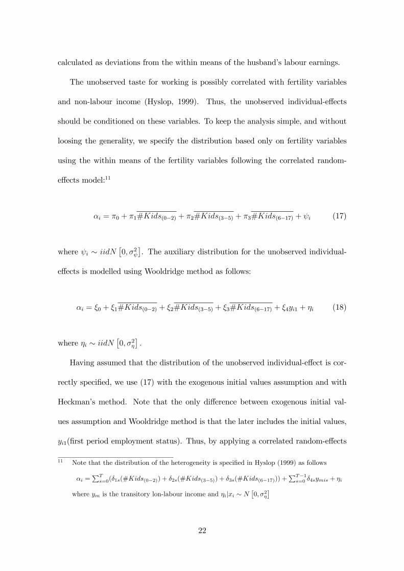
The unobserved taste for working is possibly correlated with fertility variables
and non-labour income (Hyslop, 1999). Thus, the unobserved individual-e¤ects
should be conditioned on these variables. To keep the analysis simple, and without
loosing the generality, we specify the distribution based only on fertility variables
using the within means of the fertility variables following the correlated random-
e¤ects model:11
�i = �0 + �1#Kids(0�2) + �2#Kids(3�5) + �3#Kids(6�17) + i (17)
where i � iidN�0; �2
�. The auxiliary distribution for the unobserved individual-
e¤ects is modelled using Wooldridge method as follows:
�i = �0 + �1#Kids(0�2) + �2#Kids(3�5) + �3#Kids(6�17) + �4yi1 + �i (18)
where �i � iidN�0; �2�
�:
Having assumed that the distribution of the unobserved individual-e¤ect is cor-
rectly speci�ed, we use (17) with the exogenous initial values assumption and with
Heckman�s method. Note that the only di¤erence between exogenous initial val-
ues assumption and Wooldridge method is that the later includes the initial values,
yi1(�rst period employment status). Thus, by applying a correlated random-e¤ects
11 Note that the distribution of the heterogeneity is speci�ed in Hyslop (1999) as follows
�i =PT
s=0(�1s(#Kids(0�2)) + �2s(#Kids(3�5)) + �3s(#Kids(6�17))) +PT�1
s=0 �4symis + �i
where ym is the transitory lon-labour income and �ijxi � N�0; �2�
�
22
model, we can also directly compare the results from these three approaches. The
reduced-form speci�cation for the Heckman�s method includes a constant, the ini-
tial sample values of age, age-squared, place of birth, highest level of education and
non-labour income.12
Table 7 about here
The estimation results are summarized in Table 7 by solution methods. For
brevity, the table reports results only for the true state dependence and variance
of unobserved individual-e¤ects.13 In each raw, the �rst �gure is the estimated co-
e¢ cient, the second �gure (in parentheses) is the standard error14 and the third
�gure (in brackets and bold) is the relative di¤erence between Heckman�s reduced-
form approximation and the other methods. A positive relative di¤erence repre-
sents an overestimation and a negative values is an underestimation in comparison
with the Heckman�s method.15 Additionally, in order to see the performance of the
Wooldridge method with respect to duration of the panel, we estimate the same
model with di¤erent durations from T = 3 to T = 10. In each estimation pro-
cedure, the same individuals are used and some of the explanatory variables are
12 It is important to note that the estimation results are very much dependent on the speci�cationof the reduced-form equation. In order to analyze the sensitivity of the result, we also triedwith di¤erent speci�cations of the reduced-form equation using di¤erent combinations of thepre-sample information (the di¤erent combinations of the exogenous variables). It is observedthat there are only minor changes on the true state dependence and the variance of theunobserved individual-e¤ects by adding or subtracting the variables used in the reduced-formequation.
13 The estimation results of the other parameters are not included here as there are no largeand systematic di¤erences between solution methods. However, they can be provided uponrequest from the author.
14 The standard errors are obtained by inverting the Hessian at the maximum value of thelikelihood functions.
15 Note that, here there is an intrinsic assumption that the Heckman�s approximation is thetrue method to solve the initial values problem and the performance of the other methodshas given relative to Heckman�s approximation. However, it does not mean that Heckman�smethod is actually the true method in the practice.
23

recalculated according to the duration. We also present results from pooled dy-
namic probit model (no unobserved individual-e¤ects) as a base result. It is useful
since it is not a¤ected by a misspeci�cation of unobserved individual-e¤ects.
The results produced with real data are in line with our MCE. The exogenous
initial values assumption produced very large true state dependence and very low
variance of unobserved individual-e¤ects for small samples. For instance, when T =
3, the relative di¤erence between Heckman�s method is 1:31 which means that the
exogenous initial values assumption overestimates the true state dependence almost
131% more relative to Heckman�s method. The relative di¤erence for the variance
of the unobserved individual-e¤ects is much larger. The variance of unobserved
individual-e¤ects obtained with the Heckman�s method is �ve times larger than that
of the exogenous initial values assumption for T = 3. When the duration is increased
the di¤erence decreases rapidly which is also in line with MCE. For instance, the
true state dependence is overestimated only 4% and the variance is underestimated
almost 11% for T = 10. The exogenous initial values assumption produces very
similar results with the pooled dynamic probit model when the duration is very
small. It is may be the case that the unobserved heterogeneity is underrepresented
in the short panel data sets compared to a longer one with the same individuals. It
is also observed for the long panels that the pooled dynamic probit model produces
increasingly larger persistence which is due to the lagged dependent variable. The
reason is that this model is not able to account for the persistence in the participation
sequences which is due to unobserved individual-e¤ects.
The real data performance of the Wooldridge method, in comparison with the
24

Heckman�s method, is almost the same as is in MCE. The Wooldridge method is
also not able to solve the problem of overestimation of the true state dependence and
underestimation of the variance for panels of short durations. However, the relative
di¤erence between Heckman�s method is much smaller compared to the relative
di¤erence between exogenous initial values assumption and Heckman�s method. For
T = 3, relative di¤erence is almost 12% and 22% for the true state dependence and
variance respectively. The Wooldridge method is more successful for the true state
dependence relative to variance of the unobserved individual-e¤ects. Similar to what
is found by MCE, the Wooldridge method performs as well as Heckman�s method
when the duration is larger than T = 5. All methods tend to produce similar results
for the panels of long durations.
4.2 Dynamics of the hours of work decisions of Swedish mar-
ried women,1992-2001
The second application concentrates on hours of work decisions of married women in
Sweden. Similar to the probit case, we speci�cally test whether there is signi�cant
true state dependence on the labour supply decisions after controlling for observed
and unobserved individual characteristics. The only di¤erence to the �rst empirical
application is the dependent variable. Here the dependent variable is the hours
of work decisions instead of an indicator variable representing the participation
decisions to the labour force. The hours of work data contain either a positive value
for women who are working or a zero for women who are not working. Therefore,
the hours of work data is censored below zero leading to a tobit type I speci�cation.
25

We use the same observed characteristics as the above: age, age-squared, edu-
cational status, place of birth, permanent and transitory non-labour income. The
unobserved individual-e¤ects is speci�ed as in (17) and (18), and the reduced-form
speci�cation for the Heckman�s method is the same as in the probit case.
Table 8 summarizes the results by solution methods and duration of the panel
from T = 3 to T = 10.
Table 8 about here
The impact of the initial values problem is almost the same as the above and
this result is also in line with our MCE. The exogenous initial values assumption
leads to serious bias. It overestimates the magnitude of the true state dependence
and underestimates the variance of the unobserved individual-e¤ects relative to the
Heckman�s method. We observe that the relative di¤erence is a function of the
duration of the panel data set. The Wooldridge method performs almost equally
well compared to Heckman�s method for the panels longer than T = 5 (the di¤erence
is 5 and 13 per cent), and the di¤erence is very close to zero for T = 10
5 Conclusions and discussions
The Wooldridge method is based on a very simple and novel strategy as a solu-
tion for the initial values problem in nonlinear dynamic random-e¤ects panel data
models. This character of the Wooldridge method has attracted many researchers.
However, nothing is known about its performance in comparison with the other al-
ternative Heckman�s reduced-form approximation. In this paper, using the dynamic
26
random-e¤ects probit and tobit (type I) models, the �nite sample performance of
the Wooldridge method is investigated in comparison with the ideal case in which
the initial values are known constants, the worst case which emerges with the ex-
ogenous initial values assumption, and the Heckman�s reduced-form approximation
method which is based on complicated econometric techniques. Various designs of
Monte Carlo Experiments are provided using balanced and unbalanced panel data
sets. We also provided two real data applications which concentrate on intertempo-
ral participation and hours of work decisions of married women in Sweden between
1992 and 2001.
The evidence obtained fromMCE and real data are in line with each other and
con�rmed the fact that a misspeci�cation for the conditional distribution of initial
values leads to serious bias on the magnitude of the true state dependence and the
variance of unobserved individual-e¤ects. The exogenous initial values assumption is
one of the these cases and leads to serious overestimation of the true state dependence
and serious underestimation of the variance of the unobserved individual-e¤ects.
However, this is a syndrome for small samples and the bias decrease gradually as
the duration of the panel data set increase.
We also obtain clear evidence on the performance of the Wooldridge method in
comparison with the Heckman�s method. The key parameter to select one of them
in the practice is mainly the duration of the panel data set. The Wooldridge method
does not specify an explicit conditional probability distribution for the initial values,
and the bias obtained with this method is behaviourally the same as the exogenous
initial values assumption for very short panels. The persistence which is due to
27
structural reasons is overestimated whereas the persistence due to unobserved time-
invariant individual characteristics is underestimated. However, the bias produced
by the Wooldridge method is much smaller than the bias produced by the exogenous
initial values assumption. The main message of our results is that the Wooldridge
method can be used instead of Heckman�s method only for the moderately long
panels, but for the short panels Heckman�s approximation is suggested. The other
message of the paper is very intuitive. For the panels of longer durations, the relative
importance of the initial period likelihood in the joint likelihood of all periods would
be lower leading to a lower bias which is due to the initial values problem. This is
what we observe in our MCE and real data applications that performance of all
methods tends to be equal for the panels of long durations.
References
[1] Ahrens, H. and Pincus, R. 1981. On Two Measures of Unbalancedness in a One-
way Model and Their Relation to E¢ ciency. Biometric Journal 23: 227-235.
[2] Arellano, M. and Honore, B. 2001. Panel Data Models. Some Recent Develop-
ments. Handbook of Econometrics, Vol V, Elsevier Science, Amsterdam.
[3] Arellano, M. and Bover, O. 1997. Estimating Dynamic Limited Dependent
Variable Models From Panel Data. Investigaciones Economicas 21: 141-65
28
[4] Arellano, M. and Carrasco, R. 2003. Binary Choice Panel Data Models with
Predetermined Variables. Journal of Econometrics 115: 125-157
[5] Arellano, M. and Hahn, J. 2006. Understanding Bias in Nonlinear Panel Models:
Some Recent Developments. In: R. Blundell, W. Newey, and T. Persson (eds.):
Advances in Economics and Econometrics, Ninth World Congress, Cambridge
University Press, forthcoming.
[6] Baltagi, B.H. and Chang, Y.J. 1995. Incomplete Panels. Journal of Economet-
rics 62: 67-89.
[7] Butler, J. S. and Mo¢ tt, R. 1982. A Computationally E¢ cient Quadrature
Procedure for the One-Factor Multinomial Probit Model. Econometrica 50:
761-764
[8] Blundell, R.W. and Smith, R.J. 1991. Initial Conditions and E¢ cient Esti-
mation in Dynamic Panel Data Models. Annales d�Economie et de Statistique
20/21: 109-123
[9] Bulundell, R. and Bond, S. 1998. Initial conditions and Moment Conditions in
Dynamic Panel Data Models. Journal of Econometrics 87: 115-143
[10] Card, D. and Sullivan, D., 1988. Measuring the E¤ect of Subsidized Training
Programs onMovements In and Out of Employment. Econometrica 56: 497-530
[11] Contayannis, P., Jones, A. M., and Rice, N. 2004. The dynamics of health in the
British Household Panel Survey, Journal of Applied Econometrics 19: 473-503
29
[12] Chamberlain, G. 1984. Panel Data, in Handbook of Econometrics, Vol. II, edited
by Zvi Griliches and Michael Intriligator. Amsterdam: North Holland.
[13] De Jong, R. and Herrera, A. 2005. Dynamic censored regression and the Open
Market Desk reaction function. Ohio State University and Michigan State Uni-
versity.
[14] Edin, P.A. and Fredriksson, P. 2000. �LINDA �Longitudinal INdividual DAta
for Sweden�, Working Paper 2000:19, Department of Economics, Uppsala Uni-
versity.
[15] Heckman, J.J. 1978. �Simple statistical models for discrete panel data devel-
oped and applied to test the hypothesis of true state dependence against the
hypothesis of spurious state dependence�, Annales de l�INSEE 30-31: 227-269
[16] Heckman, J.J. 1981. The Incidental Parameters Problem and the Problem of
Initial Conditions in Estimating a Discrete Time - Discrete Data Stochastic
Process, in Structural Analysis of Discrete Panel Data with Econometric Ap-
plications, ed. by C. Manski and D. McFadden, Cambridge: MIT Press.
[17] Hajivassiliou, V. and Ruud, P. 1994. Classical Estimation Methods for LDV
Models using Simulation, in R. Engle & D. McFadden, eds. Handbook of Econo-
metrics, Vol IV, 2384-2441
[18] Honore, B. 1993. Orthogonality-conditions for Tobit model with �xed e¤ect and
lagged dependent variables. Journal of Econometrics 59: 35-61
30
[19] Honore, B. 2002. Nonlinear Models with Panel Data. Portuguese Economic
Journal 1: 163�179.
[20] Honore, B. and Kryiazidou, E. 2000. Panel Data Discrete Choice Models with
Lagged Dependent Vairables. Econometrica 74: 611-629
[21] Honore, B. and Tamer, E. 2006. Bounds on Parameters in Panel Dynamic
Discrete Choice Models. Econometrica 68: 839-874
[22] Hsiao, C. 2003. Analysis of Panel Data. 2nd ed. Cambridge University Press,
Cambridge.
[23] Hu, L. 2002. Estimation of a censored dynamic panel-data model. Econometrica
70: 2499-2517
[24] Hyslop, D. R. 1999. State Dependence, Serial Correlation and Heterogeneity in
Intertemporal Labor Force Participation of Married Women. Econometrica 67:
1255�1294
[25] Gourieroux, C., and Monfort, A. 1993. Simulation-based Inference: A Survey
with Special Reference to Panel Data Models. Journal of Econometrics 59:
5-33
[26] Neyman, J. and Scott, E. 1948. Consistent Estimates Based on Partially Con-
sistent Observations. Econometrica 16: 1-32
[27] Ruud, P. 1986. Consistent estimation of limited dependent variable models
despite misspeci�cation of distribution. Journal of Econometrics 32: 157-187
31
[28] Wooldridge, J.M. 2005. Simple solutions to the initial conditions problem in
dynamic, nonlinear panel-data models with unobserved heterogeneity. Journal
of Applied Econometrics 20: 39-54
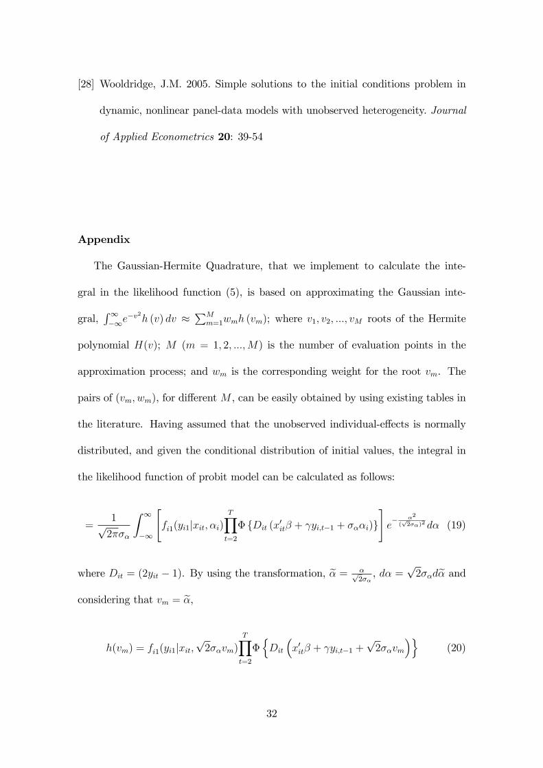
Appendix
The Gaussian-Hermite Quadrature, that we implement to calculate the inte-
gral in the likelihood function (5), is based on approximating the Gaussian inte-
gral,R1�1e
�v2h (v) dv �PM
m=1wmh (vm); where v1; v2; :::; vM roots of the Hermite
polynomial H(v); M (m = 1; 2; :::;M) is the number of evaluation points in the
approximation process; and wm is the corresponding weight for the root vm. The
pairs of (vm; wm), for di¤erent M , can be easily obtained by using existing tables in
the literature. Having assumed that the unobserved individual-e¤ects is normally
distributed, and given the conditional distribution of initial values, the integral in
the likelihood function of probit model can be calculated as follows:
=1p2���
Z 1
�1
"fi1(yi1jxit; �i)
TYt=2
� fDit (x0it� + yi;t�1 + ���i)g
#e� �2
(p2��)2 d� (19)
where Dit = (2yit � 1). By using the transformation, e� = �p2��, d� =
p2��de� and
considering that vm = e�,h(vm) = fi1(yi1jxit;
p2��vm)
TYt=2
�nDit
�x0it� + yi;t�1 +
p2��vm
�o(20)
32
The full log-likelihood function is,
LogL =NPi=1
ln
�1p�
MPm=1
wmh(vm)
�(21)
Note that the solution methods for the initial values can also be easily adopted to
the above procedure. The exogenous initial values assumption leads to ignoring
f1(:), and it can be taken outside of (19). The likelihood function for the Heckman�s
method is given as,
h(vm) = �nDi1
�zi1� +
p2���vm
�o TYt=2
�nDit
�x0it� + yi;t�1 +
p2��vm
�o(22)
and for the Wooldridge method,
h(vm) =TYt=2
�nDit
�x0it� + yi;t�1 + �0 + �1yi1 + �2xi +
p2��vm
�o(23)
The same procedure can be easily implemented for the integral which will appear in
the likelihood function of the dynamic random-e¤ects tobit model by simply using
the same strategy given the above.
33
Tab
le 1
. Res
ults
of M
CE
1: N
orm
al re
gres
sor(
True
val
ues:
11
β=
,0.
5γ
=,
1α
σ=
,1
uσ
=)
Dyn
amic
Pro
bit M
odel
Dyn
amic
Tob
it M
odel
0.5
γ=
1α
σ=
0.5
γ=
1α
σ=
TM
ean
Bia
sR
MSE
Med
ian
Bia
sM
AE
Mea
nB
ias
RM
SEM
edia
nB
ias
MA
EM
ean
Bia
sR
MSE
Med
ian
Bia
sM
AE
Mea
nB
ias
RM
SEM
edia
nB
ias
MA
E
Kno
wn
(non
stoc
hast
ic) i
nitia
l val
ues
3–0
.011
0.24
6–0
.018
0.16
3–0
.015
0.26
9–0
.042
0.17
40.
012
0.09
2
0.00
50.
061
–0.0
140.
115
–0.0
010.
071
4
0.0
080.
140
0.0
040.
091
0.0
000.
187
–0.0
380.
129
0.01
00.
060
0.00
20.
038
–0.0
090.
094
–0.0
110.
070
5
0.0
210.
125
0.0
250.
087
0.0
010.
140
0.01
80.
086
0.00
90.
049
0.01
30.
031
–0.0
090.
087
–0.0
160.
063
8
0.0
080.
093
0.01
70.
072
0.0
020.
102
0.00
40.
064
0.00
30.
029
0.00
30.
021
0.0
020.
076
–0.0
020.
049
15
0.0
140.
063
0.0
140.
047
–0.0
120.
073
–0.0
220.
045
0.0
020.
020
0.0
01 0
.014
–0.0
080.
060
–0.0
060.
036
20
0.0
090.
047
0.0
160.
040
–0.0
180.
069
–0.0
190.
041
0.0
020.
017
0.00
30.
013
–0.0
090.
060
–0.0
090.
034
Exo
geno
us in
itial
val
ues a
ssum
ptio
n3
0.
264
0.28
90.
249
0.24
9–0
.241
0.32
3–0
.243
0.25
80.
245
0.24
9
0.2
430.
243
–0.4
890.
512
–0.4
610.
461
4
0.17
50.
217
0.15
30.
153
–0.1
280.
211
–0.1
540.
182
0.18
70.
194
0.18
90.
189
–0.3
200.
341
–0.3
240.
324
5
0.11
40.
156
0.10
40.
108
–0.0
790.
156
–0.0
720.
124
0.12
70.
135
0.12
50.
125
–0.2
070.
227
–0.2
170.
217
8
0.05
30.
105
0
.050
0.06
3–0
.021
0.09
3–0
.022
0.06
90.
043
0.05
40.
049
0.04
5–0
.060
0.09
2–0
.069
0.07
515
0.
023
0.07
2 0
.020
0.05
4–0
.011
0.07
8–0
.010
0.0
57 0
.011
0.02
1 0
.011
0.0
16–0
.022
0.06
7–0
.021
0.04
420
0.
017
0.05
4 0
.019
0.04
3–0
.018
0.06
6–0
.011
0.04
9 0
.009
0.01
90.
011
0.01
5–0
.009
0.06
1–0
.010
0.03
8
Hec
kman
’s re
duce
d-fo
rm a
ppro
xim
atio
n3
0.
013
0.13
80.
012
0.07
80.
003
0.26
2–0
.017
0.15
8 0
.009
0.08
30.
019
0.06
1–0
.065
0.22
6–0
.089
0.17
14
0.
011
0.13
40.
001
0.10
0–0
.005
0.18
4–0
.026
0.15
1 0
.003
0.07
0
0.00
60.
049
–0.0
280.
162
–0.0
350.
110
5
0.00
00.
111
0.00
20.
074
–0.0
030.
142
–0.0
010.
080
0.00
80.
057
0.
015
0.03
4–0
.019
0.13
8–0
.031
0.08
98
0.
004
0.09
0
0.0
010.
056
0.00
20.
093
0
.000
0.06
60.
005
0.03
9
0.00
20.
027
–0.0
170.
126
–0.0
230.
079
15
0.00
60.
068
0.0
020.
051
–0.0
040.
077
–0.0
040.
042
–0.0
040.
029
–0.0
030.
018
–0.0
140.
094
–0.0
130.
070
20
0.00
90.
052
0.0
090.
039
–0.0
180.
066
–0.0
170.
041
–0.0
020.
024
–0.0
010.
013
–0.0
090.
093
–0.0
070.
065
Woo
ldri
dge
met
hod
3
0.16
80.
385
0.19
10.
273
–0.1
520.
467
–0.2
210.
356
0.09
80.
182
0.
084
0.12
2–0
.139
0.22
8–0
.133
0.14
94
0.
099
0.25
00.
113
0.19
5–0
.070
0.22
3–0
.107
0.15
90.
035
0.13
90.
040
0.10
2–0
.073
0.17
9–0
.054
0.12
35
0.
026
0.18
20.
045
0.14
1–0
.021
0.16
6–0
.023
0.10
40.
021
0.08
70.
018
0.06
0–0
.060
0.15
4–0
.056
0.10
28
0.
020
0.11
5
0.0
110.
067
–0.0
100.
099
–0.0
210.
061
0.00
40.
045
0.
002
0.03
4–0
.029
0.12
2–0
.026
0.07
415
0.
009
0.07
4 0
.005
0.05
2–0
.005
0.07
8–0
.008
0.0
56–0
.006
0.03
0–0
.007
0.01
8–0
.012
0.09
9–0
.019
0.07
120
0.
001
0.05
1 0
.004
0.03
6 0
.001
0.06
9 0
.009
0.05
2
0.00
10.
022
0.0
020.
014
–0.0
010.
065
–0.0
010.
055
34
Tab
le 2
. Res
ults
of M
CE2
: Non
-nor
mal
regr
esso
r(Tr
ue v
alue
s:1
1β
=,
0.5
γ=
,1
ασ
=,
1u
σ=
)D
ynam
ic P
robi
t Mod
elD
ynam
ic T
obit
Mod
el0.
5γ
=1
ασ
=0.
5γ
=1
ασ
=
TM
ean
Bia
sR
MSE
Med
ian
Bia
sM
AE
Mea
nB
ias
RM
SEM
edia
nB
ias
MA
EM
ean
Bia
sR
MSE
Med
ian
Bia
sM
AE
Mea
nB
ias
RM
SEM
edia
nB
ias
MA
E
Kno
wn
(non
stoc
hast
ic) i
nitia
l val
ues
3–0
.003
0.21
30.
005
0.15
30.
013
0.25
00.
006
0.18
1–0
.003
0.08
6–0
.005
0.04
3–0
.010
0.12
0–0
.005
0.07
14
0.0
070.
144
0.00
50.
092
0.0
110.
161
0.0
090.
106
–0.0
010.
047
–0.0
010.
030
–0.0
020.
085
–0.0
040.
065
5 0
.003
0.13
80.
004
0.08
80.
001
0.14
50.
010
0.09
2–0
.001
0.04
6 0
.001
0.03
2–0
.004
0.07
3–0
.007
0.05
58
0.0
120.
095
0.01
60.
067
0.0
150.
112
0.0
180.
062
0.0
040.
025
0.0
040.
018
–0.0
030.
072
–0.0
060.
050
15 0
.004
0.05
50.
002
0.04
3 0
.007
0.06
9 0
.009
0.04
3 0
.001
0.01
8 0
.001
0.01
4–0
.009
0.06
3–0
.003
0.03
620
0
.007
0.04
60.
008
0.04
2 0
.016
0.06
2 0
.019
0.04
2 0
.000
0.01
5–0
.001
0.01
0–0
.007
0.06
0–0
.006
0.03
5
Exo
geno
us in
itial
val
uesa
ssum
ptio
n3
0.3
090.
344
0.
305
0.30
5–0
.264
0.36
0–0
.272
0.28
50.
213
0.21
80.
211
0.21
1–0
.395
0.41
9–0
.386
0.38
64
0.2
300.
262
0.
222
0.22
2–0
.159
0.27
1–0
.183
0.20
70.
151
0.16
00.
152
0.15
2–0
.242
0.27
5–0
.252
0.25
25
0.1
480.
192
0.
132
0.13
2–0
.126
0.14
4–0
.133
0.14
40.
097
0.10
70.
100
0.10
0–0
.153
0.17
8–0
.155
0.15
58
0.0
690.
116
0.
058
0.07
5–0
.029
0.08
3–0
.035
0.04
90.
033
0.04
30.
033
0.03
4–0
.045
0.08
3–0
.054
0.06
515
0.0
160.
059
0.
020
0.04
1–0
.012
0.07
2–0
.017
0.05
00.
006
0.01
80.
008
0.01
4–0
.017
0.06
2–0
.021
0.04
120
0.0
110.
054
0.
009
0.04
0–0
.013
0.06
5–0
.018
0.04
90.
005
0.01
60.
007
0.01
0–0
.008
0.05
5–0
.011
0.03
8
Hec
kman
’sre
duce
d-fo
rmap
prox
imat
ion
3–0
.016
0.16
7–0
.001
0.09
7 0
.034
0.30
60.
025
0.18
3–0
.001
0.08
10.
002
0.04
8–0
.052
0.21
7–0
.070
0.12
84
0.0
130.
134
–0.0
050.
076
0.0
200.
217
–0.0
150.
124
0.0
030.
053
0.
006
0.03
6–0
.029
0.14
2–0
.027
0.09
65
0.0
040.
120
–0.0
010.
092
0.0
140.
121
0.0
090.
094
0.0
050.
053
0.
003
0.03
0–0
.028
0.13
7–0
.027
0.09
08
0.0
090.
091
0.0
070.
058
0.0
000.
078
–0.0
050.
054
0.0
010.
034
0.
001
0.02
1–0
.019
0.10
5–0
.017
0.07
015
–0.0
010.
056
0.0
040.
053
–0.0
080.
070
–0.0
140.
046
0
.000
0.02
8–0
.003
0.01
8–0
.005
0.09
5–0
.008
0.06
820
0.0
020.
053
–0.0
030.
039
–0.0
240.
065
–0.0
250.
047
0.0
000.
014
0.
001
0.01
2–0
.001
0.09
1–0
.003
0.06
0
Woo
ldri
dge
met
hod
30.
076
0.47
70.
075
0.23
5–0
.061
0.70
0–0
.036
0.28
00.
098
0.18
60.
110
0.13
9–0
.135
0.25
2–0
.142
0.16
34
0.07
20.
235
0.07
90.
159
–0.0
390.
284
–0.0
320.
157
0.04
70.
111
0.04
50.
074
–0.0
530.
180
–0.0
570.
131
50.
022
0.19
00.
023
0.12
0–0
.029
0.14
7–0
.025
0.08
80.
022
0.07
40.
023
0.05
1–0
.031
0.19
8–0
.037
0.10
78
0.02
10.
112
0.02
30.
081
–0.0
180.
082
–0.0
180.
051
0.0
010.
030
0.00
20.
021
–0.0
100.
103
–0.0
100.
062
15–0
.002
0.05
8–0
.001
0.03
9–0
.012
0.07
4–0
.020
0.05
2–0
.006
0.02
5–0
.006
0.01
6–0
.003
0.06
9–0
.005
0.04
320
0.00
00.
056
0.00
70.
041
–0.0
080.
064
–0.0
140.
059
–0.0
020.
015
–0.0
030.
012
0.0
010.
053
0.0
020.
039
35

Tab
le 3
. Res
ults
of M
CE
3: A
utoc
orre
late
d re
gres
sor(
True
val
ues:
11
β=
,0.
5γ
=,
1α
σ=
,1
uσ
=)
Dyn
amic
Pro
bit M
odel
Dyn
amic
Tob
it M
odel
0.5
γ=
1α
σ=
0.5
γ=
1α
σ=
TM
ean
Bia
sR
MSE
Med
ian
Bia
sM
AE
Mea
nB
ias
RM
SEM
edia
nB
ias
MA
EM
ean
Bia
sR
MSE
Med
ian
Bia
sM
AE
Mea
nB
ias
RM
SEM
edia
nB
ias
MA
E
Kno
wn
(non
stoc
hast
ic) i
nitia
l val
ues
3
0.00
80.
215
0.00
00.
125
0.03
30.
589
0.
022
0.24
1–0
.015
0.14
0–0
.017
0.09
6–0
.034
0.20
0–0
.018
0.11
44
0.
000
0.16
70.
006
0.12
20.
001
0.22
0–0
.016
0.15
0
0.0
010.
082
–0.0
030.
053
–0.0
080.
132
–0.0
110.
088
5–0
.011
0.13
0–0
.012
0.09
6–0
.009
0.14
1–0
.007
0.09
2–0
.003
0.06
5
0.
002
0.04
7–0
.015
0.12
5–0
.014
0.07
28
0
.009
0.09
3
0.
004
0.06
10.
010
0.08
7
0.0
090.
056
–0.0
050.
041
0.0
010.
030
–0.0
090.
094
–0.0
080.
063
15
0.0
100.
068
0.0
110.
045
–0.0
050.
069
–0.0
06
0.0
47
0.0
000.
023
0.
001
0.01
5–0
.015
0.08
9–0
.015
0.06
120
–0.0
020.
060
–0.0
030.
037
–0.0
120.
061
–0.0
090.
042
0
.001
0.02
1
0.
000
0.01
4–0
.010
0.08
8–0
.013
0.06
0
Exo
geno
us in
itial
val
ues a
ssum
ptio
n3
0.
258
0.30
70.
258
0.25
8–0
.222
0.76
1–0
.276
0.37
7 0
.207
0.21
4
0.
208
0.20
8–0
.438
0.48
7–0
.412
0.41
24
0.
150
0.24
50.
149
0.16
8–0
.142
0.30
4–0
.139
0.20
6 0
.143
0.15
9 0
.150
0.15
0–0
.269
0.31
9–0
.266
0.26
65
0.
110
0.20
90.
120
0.14
4–0
.057
0.25
8–0
.068
0.14
8 0
.088
0.10
4 0
.093
0.09
3–0
.154
0.20
7–0
.167
0.17
28
0.
060
0.14
1
0.0
720.
108
–0.0
310.
132
–0.0
300.
083
0.0
320.
049
0.0
340.
037
–0.0
480.
119
–0.0
420.
079
15
0.02
50.
103
0.01
50.
067
–0.0
270.
105
–0.0
20 0
.073
0
.005
0.02
8
0.00
4
0.02
2–0
.022
0.09
3–0
.024
0.06
620
0.
004
0.08
10.
008
0.05
3–0
.014
0.09
7–0
.027
0
.068
0
.002
0.02
1 0
.002
0.01
4–0
.010
0.09
2–0
.012
0.05
8
Hec
kman
’sre
duce
d-fo
rmap
prox
imat
ion
3
0.02
70.
374
0.0
450.
234
–0.0
450.
479
–0.0
380.
276
0.
001
0.08
8–0
.002
0.06
2–0
.043
0.21
9–0
.052
0.15
04
0.
022
0.28
7 0
.023
0.19
4–0
.036
0.34
9–0
.017
0.19
0–0
.003
0.06
7
0.
001
0.04
2–0
.033
0.17
4–0
.037
0.11
95
0.0
060.
247
–0.0
120.
146
–0.0
110.
267
–0.0
130.
151
0.0
040.
049
0.00
30.
033
–0.0
300.
136
–0.0
230.
081
8
0.01
70.
158
0.00
60.
097
–0.0
050.
138
–0.0
080.
091
0.0
050.
038
0.00
20.
024
–0.0
150.
111
–0.0
140.
072
15
0.00
90.
109
0.0
050.
063
–0.0
150.
107
–0.0
12 0
.072
0.0
010.
025
0.00
20.
019
–0.0
110.
095
–0.0
120.
066
20
0.00
00.
089
0.0
020.
051
–0.0
080.
099
–0.0
09 0
.068
0.0
010.
021
0.0
000.
015
–0.0
090.
089
–0.0
100.
061
Woo
ldri
dge
met
hod
3
0.05
60.
409
0.09
70.
266
–0.0
830.
451
–0.0
760.
284
0.0
440.
181
0.02
60.
108
–0.0
480.
290
–0.0
400.
191
4
0.04
20.
330
0.04
40.
208
–0.0
430.
378
–0.0
610.
231
0.
005
0.10
6 0
.004
0.07
4–0
.038
0.19
8–0
.038
0.14
05
0.0
380.
237
0.03
90.
152
–0.0
310.
273
–0.0
360.
159
0.
009
0.07
6 0
.008
0.04
6–0
.027
0.14
8–0
.028
0.09
38
0.
029
0.16
2
0.
016
0.10
0–0
.027
0.13
8–0
.014
0.08
8–0
.001
0.04
2–0
.003
0.02
8–0
.017
0.10
9–0
.011
0.07
415
0.
016
0.10
9 0
.010
0.06
2–0
.023
0.10
8–0
.018
0.
074
–0.0
030.
029
–0.0
020.
019
–0.0
160.
088
–0.0
100.
062
20
0.00
10.
089
–0.0
070.
053
–0.0
180.
098
–0.0
250.
072
0.00
00.
022
–0.0
010.
016
–0.0
110.
087
–0.0
090.
059
36
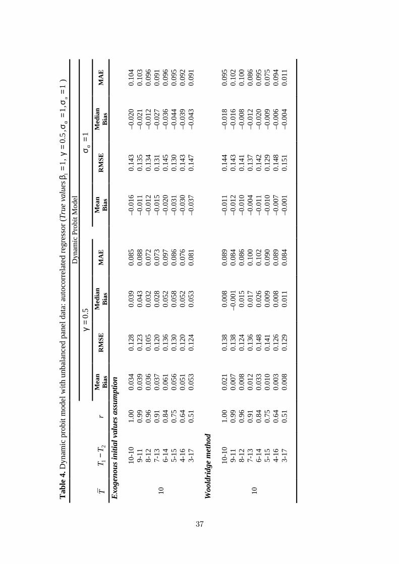
Tab
le 4
.Dyn
amic
prob
it m
odel
with
unba
lanc
ed p
anel
dat
a: a
utoc
orre
late
d re
gres
sor (
True
val
ues
11
β=
,0.
5γ
=,
1α
σ=
,1
uσ
=)
Dyn
amic
Pro
bit M
odel
0.5
γ=
1α
σ=
T2
1T
T−
rM
ean
Bia
sR
MSE
Med
ian
Bia
sM
AE
Mea
nB
ias
RM
SEM
edia
nB
ias
MA
E
Exo
geno
us in
itial
val
ues a
ssum
ptio
n
10-1
01.
000.
034
0.12
80.
039
0.08
5–0
.016
0.14
3–0
.020
0.10
49-
110.
990.
039
0.12
30.
043
0.08
8–0
.011
0.13
5–0
.021
0.10
38-
120.
960.
036
0.10
50.
032
0.07
2–0
.012
0.13
4–0
.012
0.09
67-
130.
910.
037
0.12
00.
028
0.07
3–0
.015
0.13
1–0
.027
0.09
16-
140.
840.
061
0.13
60.
052
0.09
7–0
.020
0.14
5–0
.036
0.09
65-
150.
750.
056
0.13
00.
058
0.08
6–0
.031
0.13
0–0
.044
0.09
54-
160.
640.
051
0.12
00.
052
0.07
6–0
.030
0.14
3–0
.039
0.09
2
10
3-17
0.51
0.05
30.
124
0.05
30.
081
–0.0
370.
147
–0.0
430.
091
Woo
ldri
dge
met
hod
10-1
01.
000.
021
0.13
80.
008
0.08
9–0
.011
0.14
4–0
.018
0.09
59-
110.
990.
007
0.13
8–0
.001
0.08
4–0
.012
0.14
3–0
.016
0.10
28-
120.
960.
008
0.12
40.
015
0.08
6–0
.010
0.14
1–0
.008
0.10
07-
130.
910.
012
0.13
60.
017
0.10
0–0
.004
0.13
7–0
.012
0.08
66-
140.
840.
033
0.14
80.
026
0.10
2–0
.011
0.14
2–0
.020
0.09
55-
150.
750.
010
0.14
10.
009
0.09
0–0
.010
0.12
9–0
.009
0.07
54-
160.
640.
003
0.12
60.
008
0.08
9–0
.007
0.14
8–0
.006
0.09
4
10
3-17
0.51
0.00
80.
129
0.01
10.
084
–0.0
010.
151
–0.0
040.
011
37
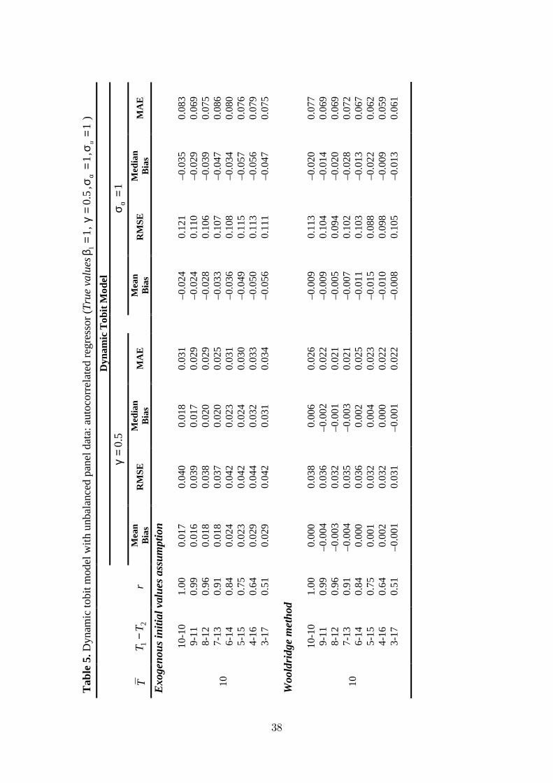
Tab
le 5
.Dyn
amic
tobi
t mod
el w
ithun
bala
nced
pan
el d
ata:
aut
ocor
rela
ted
regr
esso
r (Tr
ue v
alue
s1
1β
=,
0.5
γ=
,1
ασ
=,
1u
σ=
)D
ynam
ic T
obit
Mod
el0.
5γ
=1
ασ
=
T2
1T
T−
rM
ean
Bia
sR
MSE
Med
ian
Bia
sM
AE
Mea
nB
ias
RM
SEM
edia
nB
ias
MA
E
Exo
geno
us in
itial
val
ues a
ssum
ptio
n
10-1
01.
000.
017
0.04
00.
018
0.03
1–0
.024
0.12
1–0
.035
0.08
39-
110.
990.
016
0.03
90.
017
0.02
9–0
.024
0.11
0–0
.029
0.06
98-
120.
960.
018
0.03
80.
020
0.02
9–0
.028
0.10
6–0
.039
0.07
57-
130.
910.
018
0.03
70.
020
0.02
5–0
.033
0.10
7–0
.047
0.08
66-
140.
840.
024
0.04
20.
023
0.03
1–0
.036
0.10
8–0
.034
0.08
05-
150.
750.
023
0.04
20.
024
0.03
0–0
.049
0.11
5–0
.057
0.07
64-
160.
640.
029
0.04
40.
032
0.03
3–0
.050
0.11
3–0
.056
0.07
9
10
3-17
0.51
0.02
90.
042
0.03
10.
034
–0.0
560.
111
–0.0
470.
075
Woo
ldri
dge
met
hod
10-1
01.
000.
000
0.03
80.
006
0.02
6–0
.009
0.11
3–0
.020
0.07
79-
110.
99–0
.004
0.03
6–0
.002
0.02
2–0
.009
0.10
4–0
.014
0.06
98-
120.
96–0
.003
0.03
2–0
.001
0.02
1–0
.005
0.09
4–0
.020
0.06
97-
130.
91–0
.004
0.03
5–0
.003
0.02
1–0
.007
0.10
2–0
.028
0.07
26-
140.
840.
000
0.03
60.
002
0.02
5–0
.011
0.10
3–0
.013
0.06
75-
150.
750.
001
0.03
20.
004
0.02
3–0
.015
0.08
8–0
.022
0.06
24-
160.
640.
002
0.03
20.
000
0.02
2–0
.010
0.09
8–0
.009
0.05
9
10
3-17
0.51
–0.0
010.
031
–0.0
010.
022
–0.0
080.
105
–0.0
130.
061
38
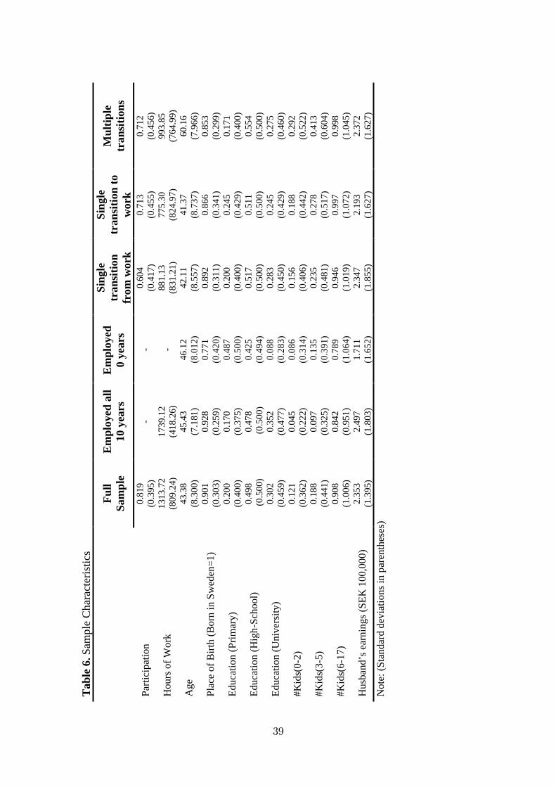
Tab
le6.
Sam
ple
Cha
ract
eris
tics
Full
Sam
ple
Em
ploy
ed a
ll10
yea
rsE
mpl
oyed
0 ye
ars
Sing
letr
ansi
tion
from
wor
k
Sing
letr
ansi
tion
tow
ork
Mul
tiple
tran
sitio
ns
Parti
cipa
tion
0.81
9(0
.395
)-
-0.
604
(0.4
17)
0.71
3(0
.455
)0.
712
(0.4
56)
Hou
rs o
f Wor
k13
13.7
2(8
09.2
4)17
39.1
2(4
18.2
6)-
881.
13(8
31.2
1)77
5.30
(824
.97)
993.
85(7
64.9
9)
Age
43.3
8(8
.300
)45
.43
(7.1
81)
46.1
2(8
.012
)42
.11
(8.5
57)
41.3
7(8
.737
)60
.16
(7.9
66)
Plac
e of
Birt
h (B
orn
in S
wed
en=1
)0.
901
(0.3
03)
0.92
8(0
.259
)0.
771
(0.4
20)
0.89
2(0
.311
)0.
866
(0.3
41)
0.85
3(0
.299
)
Educ
atio
n (P
rimar
y)0.
200
(0.4
00)
0.17
0(0
.375
)0.
487
(0.5
00)
0.20
0(0
.400
)0.
245
(0.4
29)
0.17
1(0
.400
)
Educ
atio
n (H
igh-
Scho
ol)
0.49
8 (0
.500
)0.
478
(0.5
00)
0.42
5(0
.494
)0.
517
(0.5
00)
0.51
1(0
.500
)0.
554
(0.5
00)
Educ
atio
n (U
nive
rsity
)0.
302
(0.4
59)
0.35
2(0
.477
)0.
088
(0.2
83)
0.28
3(0
.450
)0.
245
(0.4
29)
0.27
5(0
.460
)
#Kid
s(0-
2)0.
121
(0.3
62)
0.04
5(0
.222
)0.
086
(0.3
14)
0.15
6(0
.406
)0.
188
(0.4
42)
0.29
2(0
.522
)
#Kid
s(3-
5)0.
188
(0.4
41)
0.09
7(0
.325
)0.
135
(0.3
91)
0.23
5(0
.481
)0.
278
(0.5
17)
0.41
3(0
.604
)
#Kid
s(6-
17)
0.90
8(1
.006
)0.
842
(0.9
51)
0.78
9(1
.064
)0.
946
(1.0
19)
0.99
7(1
.072
)0.
998
(1.0
45)
Hus
band
’s e
arni
ngs(
SEK
100
,000
)2.
353
(1.3
95)
2.49
7(1
.803
)1.
711
(1.6
52)
2.34
7(1
.855
)2.
193
(1.6
27)
2.37
2(1
.627
)N
ote:
(Sta
ndar
d de
viat
ions
in p
aren
thes
es)
39
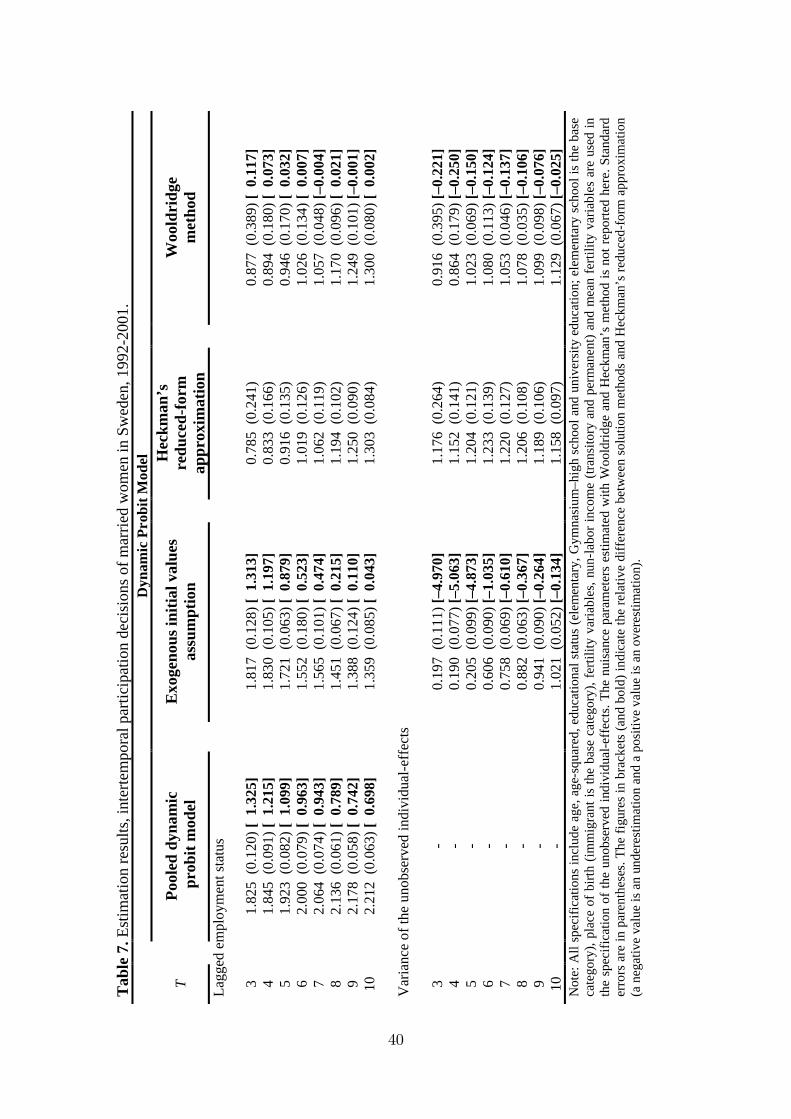
Tab
le7.
Est
imat
ion
resu
lts, i
nter
tem
pora
l par
ticip
atio
n de
cisi
ons o
f mar
ried
wom
en in
Sw
eden
, 199
2-20
01.
Dyn
amic
Pro
bit M
odel
TPo
oled
dyna
mic
prob
itm
odel
Exo
geno
us in
itial
val
ues
assu
mpt
ion
Hec
kman
’sre
duce
d-fo
rmap
prox
imat
ion
Woo
ldri
dge
met
hod
Lagg
edem
ploy
men
t sta
tus
31.
825
(0.1
20)[
1.3
25]
1.81
7 (0
.128
)[ 1
.313
]0.
785
(0.2
41)
0.87
7 (0
.389
)[ 0
.117
]4
1.84
5 (0
.091
)[ 1
.215
]1.
830
(0.1
05)[
1.1
97]
0.83
3 (0
.166
)0.
894
(0.1
80)[
0.0
73]
51.
923
(0.0
82)[
1.0
99]
1.72
1 (0
.063
)[ 0
.879
]0.
916
(0.1
35)
0.94
6 (0
.170
)[ 0
.032
]6
2.00
0 (0
.079
)[ 0
.963
]1.
552
(0.1
80)[
0.5
23]
1.01
9 (0
.126
)1.
026
(0.1
34)[
0.0
07]
72.
064
(0.0
74)[
0.9
43]
1.56
5 (0
.101
)[ 0
.474
]1.
062
(0.1
19)
1.05
7 (0
.048
)[–0
.004
]8
2.13
6 (0
.061
)[ 0
.789
]1.
451
(0.0
67)[
0.2
15]
1.19
4 (0
.102
)1.
170
(0.0
96)[
0.0
21]
92.
178
(0.0
58)[
0.7
42]
1.38
8 (0
.124
)[ 0
.110
]1.
250
(0.0
90)
1.24
9 (0
.101
)[–0
.001
]10
2.21
2 (0
.063
)[ 0
.698
]1.
359
(0.0
85)[
0.0
43]
1.30
3 (0
.084
)1.
300
(0.0
80)[
0.0
02]
Var
ianc
e of
the
unob
serv
ed in
divi
dual
-eff
ects
3-
0.19
7 (0
.111
)[–4
.970
]1.
176
(0.2
64)
0.91
6 (0
.395
)[–0
.221
]4
-0.
190
(0.0
77)[
–5.0
63]
1.15
2 (0
.141
)0.
864
(0.1
79)[
–0.2
50]
5-
0.20
5 (0
.099
)[–4
.873
]1.
204
(0.1
21)
1.02
3 (0
.069
)[–0
.150
]6
-0.
606
(0.0
90)[
–1.0
35]
1.23
3 (0
.139
)1.
080
(0.1
13)[
–0.1
24]
7-
0.75
8 (0
.069
)[–0
.610
]1.
220
(0.1
27)
1.05
3 (0
.046
)[–0
.137
]8
-0.
882
(0.0
63)[
–0.3
67]
1.20
6 (0
.108
)1.
078
(0.0
35)[
–0.1
06]
9-
0.94
1 (0
.090
)[–0
.264
]1.
189
(0.1
06)
1.09
9 (0
.098
)[–0
.076
]10
-1.
021
(0.0
52)[
–0.1
34]
1.15
8 (0
.097
)1.
129
(0.0
67)[
–0.0
25]
Not
e: A
ll sp
ecifi
catio
ns in
clud
e ag
e, a
ge-s
quar
ed, e
duca
tiona
l sta
tus
(ele
men
tary
, Gym
nasi
um–h
igh
scho
ol a
nd u
nive
rsity
edu
catio
n;el
emen
tary
sch
ooli
sth
e ba
seca
tego
ry),
plac
e of
birt
h (im
mig
rant
is th
e ba
se c
ateg
ory)
, fer
tility
var
iabl
es, n
un-la
bor i
ncom
e (tr
ansi
tory
and
per
man
ent)
and
mea
n fe
rtilit
y va
riabl
esar
eus
ed in
the
spec
ifica
tion
of th
e un
obse
rved
indi
vidu
al-e
ffec
ts. T
he n
uisa
nce
para
met
ers
estim
ated
with
Woo
ldrid
ge a
nd H
eckm
an’s
met
hod
is n
ot re
porte
d he
re.S
tand
ard
erro
rs a
re in
par
enth
eses
. The
figu
res
in b
rack
ets
(and
bol
d) in
dica
te th
ere
lativ
edi
ffer
ence
bet
wee
nso
lutio
n m
etho
ds a
ndH
eckm
an’s
redu
ced-
form
app
roxi
mat
ion
(a n
egat
ive
valu
e is
an
unde
rest
imat
ion
and
a po
sitiv
e va
lue
is a
n ov
eres
timat
ion)
.
40
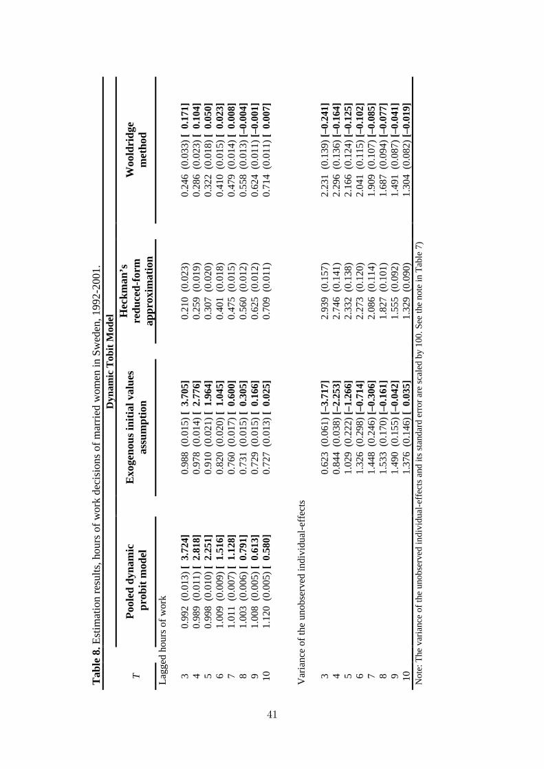
Tab
le8.
Est
imat
ion
resu
lts,h
ours
of w
ork
deci
sion
s of m
arrie
d w
omen
in S
wed
en, 1
992-
2001
.D
ynam
ic T
obit
Mod
el
TPo
oled
dyna
mic
prob
itm
odel
Exo
geno
us in
itial
val
ues
assu
mpt
ion
Hec
kman
’sre
duce
d-fo
rmap
prox
imat
ion
Woo
ldri
dge
met
hod
Lagg
edho
urs o
f wor
k
30.
992
(0.0
13)[
3.7
24]
0.98
8 (0
.015
)[ 3
.705
]0.
210
(0.0
23)
0.24
6 (0
.033
)[ 0
.171
]4
0.98
9 (0
.011
)[ 2
.818
]0.
978
(0.0
14)[
2.7
76]
0.25
9 (0
.019
)0.
286
(0.0
23)[
0.1
04]
50.
998
(0.0
10)[
2.2
51]
0.91
0 (0
.021
)[ 1
.964
]0.
307
(0.0
20)
0.32
2 (0
.018
)[ 0
.050
]6
1.00
9 (0
.009
)[ 1
.516
]0.
820
(0.0
20)[
1.0
45]
0.40
1 (0
.018
)0.
410
(0.0
15)[
0.0
23]
71.
011
(0.0
07)[
1.1
28]
0.76
0 (0
.017
)[ 0
.600
]0.
475
(0.0
15)
0.47
9 (0
.014
)[ 0
.008
]8
1.00
3 (0
.006
)[ 0
.791
]0.
731
(0.0
15)[
0.3
05]
0.56
0 (0
.012
)0.
558
(0.0
13)[
–0.0
04]
91.
008
(0.0
05)[
0.6
13]
0.72
9 (0
.015
)[ 0
.166
]0.
625
(0.0
12)
0.62
4 (0
.011
)[–0
.001
]10
1.12
0 (0
.005
)[ 0
.580
]0.
727
(0.0
13)[
0.0
25]
0.70
9 (0
.011
)0.
714
(0.0
11)[
0.0
07]
Var
ianc
e of
the
unob
serv
ed in
divi
dual
-eff
ects
30.
623
(0.0
61)[
–3.7
17]
2.93
9 (0
.157
)2.
231
(0.1
39)[
–0.2
41]
40.
844
(0.0
38)[
–2.2
53]
2.74
6 (0
.141
)2.
296
(0.1
36)[
–0.1
64]
51.
029
(0.2
22)[
–1.2
66]
2.33
2 (0
.138
)2.
166
(0.1
24)[
–0.1
25]
61.
326
(0.2
98)[
–0.7
14]
2.27
3 (0
.120
)2.
041
(0.1
15)[
–0.1
02]
71.
448
(0.2
46)[
–0.3
06]
2.08
6 (0
.114
)1.
909
(0.1
07)[
–0.0
85]
81.
533
(0.1
70)[
–0.1
61]
1.82
7 (0
.101
)1.
687
(0.0
94)[
–0.0
77]
91.
490
(0.1
55)[
–0.0
42]
1.55
5 (0
.092
)1.
491
(0.0
87)[
–0.0
41]
101.
376
(0.1
46)[
0.0
35]
1.32
9 (0
.090
)1.
304
(0.0
82)[
–0.0
19]
Not
e:Th
e va
rianc
e of
the
unob
serv
ed in
divi
dual
-eff
ects
and
its s
tand
ard
erro
r are
scal
ed b
y 10
0. S
ee th
e no
te in
Tab
le 7
)
41