LIMS-2021-12

The World in a Grain of Sand: Condensing the String Vacuum Degeneracy

Yang-Hui He,1, 2, 3, 4 Shailesh Lal,5 and M. Zaid Zaz6

1London Institute, Royal Institution of GB, 21 Albemarle St., London W1S 4BS2Merton College, University of Oxford, OX1 4JD, UK

3Department of Mathematics, City, University of London, London EC1V0HB, UK4School of Physics, NanKai University, Tianjin, 300071, P.R. China∗

5Faculdade de Ciencias, Universidade do Porto, 687 Rua do Campo Alegre, Porto, Portugal†

6Department of Physics & Astronomy, University of Nebraska, Lincoln, NE 68588-0299, USA‡

We propose a novel approach toward the vacuum degeneracy problem of the string landscape, byfinding an efficient measure of similarity amongst compactification scenarios. Using a class of someone million Calabi-Yau manifolds as concrete examples, the paradigm of few-shot machine-learningand Siamese Neural Networks represents them as points in R3 where the similarity score betweentwo manifolds is the Euclidean distance between their R3 representatives. Using these methods, wecan compress the search space for exceedingly rare manifolds to within one percent of the originaldata by training on only a few hundred data points. We also demonstrate how these methods maybe applied to characterize ‘typicality’ for vacuum representatives.

I. INTRODUCTION AND SUMMARY

The biggest theoretical challenge to string/M-theorybeing “the theory of everything” is the proliferation ofpossible low-energy, 4-dimensional solutions akin to ouruniverse. The plethora of possibilities in reducing thehigh space-time dimensions - where gravity and quantumfield theory unify - gives rise to such astronomical num-bers as the often-quoted 10500 in compactification scenar-ios [1] as well as more recent and much larger estimates[2, 3]. While constraints such as exact Standard Modelparticle spectrum place severe reduction on the allowedlandscape of vacua [4–9], such reductions are typically onthe order of 1 in 1010 and are but a drop in the ocean.

Confronted with this vastness, a key resolution wouldbe the identification of a measure on the landscape,so that oases of phenomenologically viable universesare favoured, while deserts of inconsistent realities areslighted. Such statistical approaches were undertakenin [10], even before exact string standard models werefound. Nevertheless, finding such a measure, givinghow close one compactification scenario is to another -whereby giving hope of vastly reducing the degeneracyof the string landscape - still remains a conceptual andcomputational puzzle.

The zeitgeist of artificial intelligence (AI) has en-gendered the almost inevitable introduction of machinelearning (ML) in the exploration of the landscape ofvacua 1 [11–13] (q.v. [14–17]), and indeed, of mathemat-ical structures in general [18] (q.v. [19, 20] for reviews).

∗ hey@maths.ox.ac.uk† shailesh.hri@gmail.com‡ zzaz2@huskers.unl.edu1 Indeed, the current state of our knowledge of the string land-

scape is very similar to a typical semi-supervised learning prob-lem, where one has at hand a minimal amount of human expert

The typical approach adopted in these studies is to feedlandscape data into an ML framework and pose questionseither as classifications (e.g., [11, 16, 21–23]) or regres-sions (e.g., [24]), or to use reinforcement learning [25–28]to formulate optimal strategies for arriving at both topdown and bottom up models of particle phenomenology.

This letter shows, using concrete examples, that MLprovides a natural and direct incursion onto the degener-acy problem, using the powerful paradigm of similarity,via so-called Siamese neural networks (SNNs) [29, 30], anarchitecture precisely designed for similarity of elementsof a dataset 2. In addition, SNNs possess two powerfulproperties of great help in our analyses of landscape ex-ploration: (1) few shot learning, which evades the needfor significant amount of training data, and (2) super-vised clustering [32], which explicitly realizes the similar-ity measure. In particular, the the NN learns a repre-sentation of input data into an embedding space where“similar” points are close together with respect to theusual Euclidean distance 3 .

This similarity principle is our saving grace from thelack of a vacuum selection principle: given two compact-ification scenarios, a similarity score gives a measure onthe landscape. Thus, whether a vacuum solution is phe-nomenologically viable can be decided by fiat and the“des res” [7] of our universe can be selected, wherebycompressing the vastness of the landscape into typicalrepresentatives.

labeled data and the bulk of the data is unlabeled. The methodsoutlined in this paper, especially in Section IV B, may also beregarded as a natural starting point for such analyses.

2 Recently [31], SNNs were used to characterize symmetry in phys-ical systems.

3 The clustering is ‘supervised’ because as instances of similar anddissimilar pairs are explicitly supplied to the ML algorithm. Thisis in contrast, for instance, to the unsupervised clustering of [17].

arX

iv:2

111.

0476

1v1

[he

p-th

] 8

Nov

202

1

2

FIG. 1: The ‘features’ network. The convolutional layers enable the extraction of local features from CICY images.

We provide here a concrete proof-of-concept of thisidea using explicit data, viz., what was referred to as“landscape data” in [11, 12] We will focus on the so-calledcomplete intersection Calabi-Yau (CICY) manifolds incomplex dimension three [33–36] and four [37, 38], whichare chosen for their deep relevance to foundational prob-lems in algebraic geometry and string theory [23, 39–41]as well as the proven effectiveness of AI/ML methods inanalyzing these datasets [11, 12, 21, 22, 42–44]. Thesetwo datasets will be our representative “landscape” 4.By clustering with similarity, one may hope to identifysubsets of data which are very likely to yield a giventopology, and conversely exclude those subsets which arenot. In short, we are attempting to few-shot learn thestring landscape.

This letter is organized as follows. We begin by intro-ducing the landscape data and their representations in§II and how SNNs address them in §III. The results arepresented in §IV and conclusions with outlook, in §V.

II. REPRESENTING THE LANDSCAPE

The key point to our methodology is that a CICYcan be realized as an integer matrix, which encodes the(multi-)degrees of the defining polynomials in some ap-propriate ambient space, see e.g. the recent textbook[45]. While we relegate details to Appendix A, the up-shot is that for the purposes of computing topologicalquantities, a CICY is the matrix

M =

q11 q21 . . . qk1q12 q22 . . . qk2...

.... . .

...q1m q2m . . . qkm

m∑i=1

k∑j=1

qji = k +D +m ,

(II.1)

4 Indeed, apart from their direct relevance to string phenomenol-ogy – the Hodge numbers determine the spectrum of masslessfermions in the string compactification – these datasets also ex-plicitly realize the general spirit of the landscape problem. Thecomputation of the Hodge numbers is a complicated problemwhose difficulty is further exacerbated by the sheer number ofcases for which this must be done. This, in a nutshell, is thestring landscape problem.

where qji ∈ Z≥0 and D is the (complex) dimension of themanifold M , which for us will be 3 or 4, to whcih we willrefer as CICY3 and CICY4 respectively.

One of the key problems in algebraic geometry, and inparallel, in string theory, is to compute topological quan-tities 5 from M . Such topological quantities will governsuch important properties such as fundamental standard-model particles. Indeed, the paradigm of string theoryis that the geometry of compactification manifolds suchas M determines the physics of the macroscopic (3 + 1)-dimensions of spacetime. The most famous of such atopological quantity is the so-called Hodge number, acomplex generalization of Betti numbers which count thenumber of “holes” of various dimension in M . There aremultiple Hodge numbers for Calabi-Yau manifolds of di-mension D and since the early days of string phenomenol-ogy, these quantities have been interpreted as dictatingthe particle content of the compactification of string the-ory to low-energy standard model [47]. We will largelyfocus on the positive integer h1,1 throughout this letter.Thus, the model for our “landscape” will be labelled dataof the form

(qij) −→ h1,1 , (II.2)

where the criterion for similarity ∼ is

q(A) ∼ q(B) iff h1,1(A) = h1,1(B) , (II.3)

between two CICY matrices labeled by (A) and (B). Weemphasize that our methodology is general and one couldchoose any other quantity of geometrical and phenomeno-logical interest to label the data.

The demographics of the CICY datasets are outlinedin the Supplementary Materials (Section and Figs there).We note here that the CICY3 dataset consists of 7890matrices corresponding to 18 distinct values of h whilethe CICY four-fold dataset is much larger, with 905684non-trivial entries and 23 distinct values of h. An im-portant hindrance in the study of either dataset is its ex-treme skewness, with the tails of allowed h values sparsely

5 Another reason why so much work so far has been focused ontopological quantities is that no explicit compact Calabi-Yaumetric has been found so far. We refer the reader to the recentinteresting numerical work [46] in this regard.

3

populated, while the middle is densely populated. In-deed, this skewness characterizes every known landscapedataset [20].

A possible way of addressing this skewness is to con-struct synthetic data for the sparely populated classes ala [43]. Few shot learning enables us to go in a com-plementary direction, where we aggressively reduce thenumber of elements we need for training, even for denselypopulated classes. Indeed, to learn the 7890 elements ofCICY3 and 905684 elements of CICY4 we draw on merely2.67% and 0.62% of the full datasets, respectively 6.

Finally, since the CICY matrices have variable shape,with entries ranging from 1×1 (the famous quintic three-fold) to 15×18, we uniformize the input data by resizingeach matrix to a uniform size n× n as described in Ap-pendix B 2. This uniformization further removes explicitinformation about the number of rows and columns in agiven CICY matrix. Since a large portion of the datasetsare favorable, i.e. the Hodge number h1,1 equals the num-ber of rows in the matrix, this step also guards against theSNN learning spurious correlations between the matrixsize and Hodge number. As a further check, we find sim-ilar results when uniformizing bi-linear interpolation [48]which is a completely different approach from paddingand washes out any favourability information.

III. METHODOLOGY

As mentioned in the Introduction, there is tremendousdifficulty but uttermost importance in defining an appro-priate distance in the landscape, even theoretically, so asto identify the “typical” vacuum or the “similarity” be-tween vacua. The key element with which an SNN solvesthis problem is is a so-called Features Network (FN). Thisimplements a map φw from elements of a dataset D toRd. Here w denote the weights and biases of the FN andwe set d = 3 below. The desired property of the mapφw, visualized in Figure 2 is that similar elements of Dare mapped close together, and dissimilar elements aremapped far apart. The w are determined by extremizinga loss function dependent on

dw (x1, x2) ≡ (φw (x1)− φw (x2))2, (III.1)

the squared Euclidean distance between the representa-tive points of data elements x1 and x2. There are multi-ple options for the loss function, starting with the orig-inal approach of [29, 30], and we adopt the triplet lossfunction given by [49, 50]

L (w) = max {dw(xa, xp)− dw(xa, xn) + 1, 0} , (III.2)

6 These amounts are split into Train and Validation subsets forthe SNN training. More details are in the Appendix B 1.

Rd

xa

xp

xn

φw(xa)φw(xp)

φw(xn)D

φw

φw

φw

FIG. 2: The mapping φw : D → Rd learnt by thefeatures network. Similar images A, P map close

together while the dissimilar image N maps far away.

where xa is a reference ‘anchor’ CICY matrix, xp is a‘positive’ CICY matrix with the same h as xa, and xn isa ‘negative’ CICY matrix with a different h. Minimizingthis loss in w leads to learning an embedding φw suchthat similar data cluster together and the dissimilar dataare pushed apart. The dw in (III.1) is then interpretedas our desired similarity score.

The input data of n×n real values matrices have a nat-ural interpretation as pixelated images, where the (i, j)-th pixel is coloured according to qij in grey-scale. Ourfeatures network, Figure 1, exploits this “image” repre-sentation by incorporating elements from computer vi-sion architectures, principally, convolutional layers. Theresulting network is called a convolutional neural networkor a ConvNet, and is briefly reviewed in the Appendix C.

Note: We may also, inspired by [21, 22], design thefeatures network using simplified versions of the Incep-tion [51, 52] and Residual [53] blocks. This yields compa-rable results, and we focus on the ConvNet for simplicity.

IV. RESULTS & DISCUSSION

We now evaluate the trained SNN by computing sim-ilarity scores across the test set, which, we recall are97.82% and 99.38% of the entire CICY3 and CICY4data respectively. Mean similarity scores for each pairof Hodge numbers h1,1 from these test sets are displayedin Figures 3 and 4. We see that the similarity scoresalong the diagonal (i.e. for matrices belonging to thesame h1,1) are concentrated close to 0, while scores fordissimilar matrices are concentrated away from 0, whichwas indeed our criterion for the putative similarity mea-sure. Put together, these figures explicitly demonstratefew shot learning ; the SNNs have been trained on ex-tremely sparse data, sometimes just 3 from each class(see Tables I and II). Despite this extreme paucity oftraining data, the SNNs learn a similarity score that isrepresentative of the full datasets. The representationof the dataset learned by the Siamese net in the embed-ding space R3 is shown in Figures 5 and 6 where we see

4

FIG. 3: The similarity score for three-folds.

FIG. 4: The similarity score for four-folds.

that CICY matrices belonging to the same h1,1 tend tocluster together.

FIG. 5: CICY Three-folds visualized by the SNN. Thecolor scheme is h1,1.

FIG. 6: CICY four-folds as visualized by the SNN. Thecolor scheme is h1,1.

A. Clustering CICY Manifolds

We now apply these results to identify subsets of CI-CYs that are likely to contain given h1,1 values. Suchcomputations provide a paradigm to isolate regions of thestring landscape by their likelihood to contain standard-model-like vacua. The precise choice of these regions issomewhat subtle, and depends on the confidence withwhich we would like to select/reject manifolds in thelandscape. For illustration, we train a Nearest Neigh-bors Classifier on the embedding space representationslearnt by FN for CICY3 and CICY4 respectively.

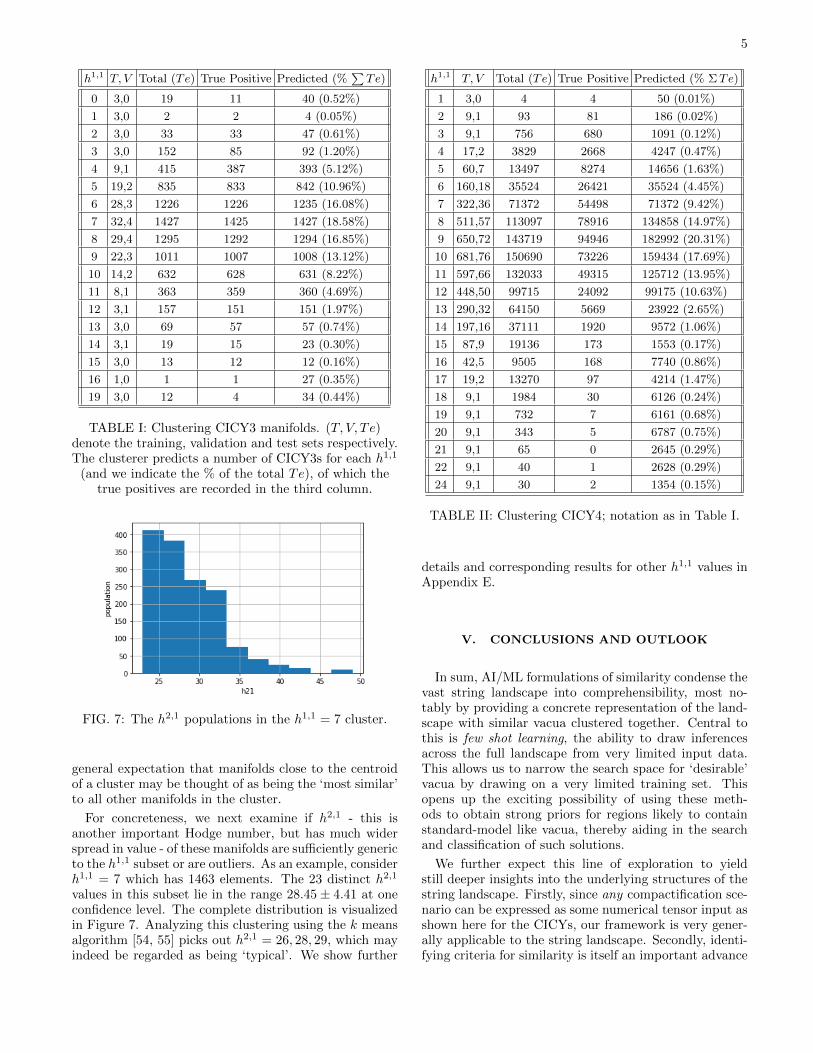
Our results in Tables I and II demonstrate that theSNN hones into relatively tiny regions of the landscapewhere these manifolds are most likely to be found. In allcases but for h1,1 = 21 for CICY4, the clustering is sig-nificantly better than random choice. As an example, theh1,1 = 4 subclass for the CICY4 test set corresponds to3829 manifolds out of the total 901099. Identifying evenone manifold from this subset correctly by random guess-ing is extremely unlikely. In contrast, the above classifierpredicts 4247 manifolds as corresponding to h1,1 = 4,which is correct for 2668 of these. Thus, the learnedsimilarity score dramatically reduces the search space ofh1,1 = 4 CICY4s from 901099 to 4247 ‘most likely’ man-ifolds.

B. Typical h2,1s for CICY3s

The SNN has been trained above on a particular crite-rion of similarity, namely, the matching of h1,1. We nowexamine how the clustering learned by the SNN may beinterpreted to reflect a still broader notion of similarityin the dataset. To define this question, we start from the

5

h1,1 T, V Total (Te) True Positive Predicted (%∑Te)

0 3,0 19 11 40 (0.52%)

1 3,0 2 2 4 (0.05%)

2 3,0 33 33 47 (0.61%)

3 3,0 152 85 92 (1.20%)

4 9,1 415 387 393 (5.12%)

5 19,2 835 833 842 (10.96%)

6 28,3 1226 1226 1235 (16.08%)

7 32,4 1427 1425 1427 (18.58%)

8 29,4 1295 1292 1294 (16.85%)

9 22,3 1011 1007 1008 (13.12%)

10 14,2 632 628 631 (8.22%)

11 8,1 363 359 360 (4.69%)

12 3,1 157 151 151 (1.97%)

13 3,0 69 57 57 (0.74%)

14 3,1 19 15 23 (0.30%)

15 3,0 13 12 12 (0.16%)

16 1,0 1 1 27 (0.35%)

19 3,0 12 4 34 (0.44%)

TABLE I: Clustering CICY3 manifolds. (T, V, Te)denote the training, validation and test sets respectively.The clusterer predicts a number of CICY3s for each h1,1

(and we indicate the % of the total Te), of which thetrue positives are recorded in the third column.

FIG. 7: The h2,1 populations in the h1,1 = 7 cluster.

general expectation that manifolds close to the centroidof a cluster may be thought of as being the ‘most similar’to all other manifolds in the cluster.

For concreteness, we next examine if h2,1 - this isanother important Hodge number, but has much widerspread in value - of these manifolds are sufficiently genericto the h1,1 subset or are outliers. As an example, considerh1,1 = 7 which has 1463 elements. The 23 distinct h2,1

values in this subset lie in the range 28.45± 4.41 at oneconfidence level. The complete distribution is visualizedin Figure 7. Analyzing this clustering using the k meansalgorithm [54, 55] picks out h2,1 = 26, 28, 29, which mayindeed be regarded as being ‘typical’. We show further

h1,1 T, V Total (Te) True Positive Predicted (% ΣTe)

1 3,0 4 4 50 (0.01%)

2 9,1 93 81 186 (0.02%)

3 9,1 756 680 1091 (0.12%)

4 17,2 3829 2668 4247 (0.47%)

5 60,7 13497 8274 14656 (1.63%)

6 160,18 35524 26421 35524 (4.45%)

7 322,36 71372 54498 71372 (9.42%)

8 511,57 113097 78916 134858 (14.97%)

9 650,72 143719 94946 182992 (20.31%)

10 681,76 150690 73226 159434 (17.69%)

11 597,66 132033 49315 125712 (13.95%)

12 448,50 99715 24092 99175 (10.63%)

13 290,32 64150 5669 23922 (2.65%)

14 197,16 37111 1920 9572 (1.06%)

15 87,9 19136 173 1553 (0.17%)

16 42,5 9505 168 7740 (0.86%)

17 19,2 13270 97 4214 (1.47%)

18 9,1 1984 30 6126 (0.24%)

19 9,1 732 7 6161 (0.68%)

20 9,1 343 5 6787 (0.75%)

21 9,1 65 0 2645 (0.29%)

22 9,1 40 1 2628 (0.29%)

24 9,1 30 2 1354 (0.15%)

TABLE II: Clustering CICY4; notation as in Table I.

details and corresponding results for other h1,1 values inAppendix E.

V. CONCLUSIONS AND OUTLOOK

In sum, AI/ML formulations of similarity condense thevast string landscape into comprehensibility, most no-tably by providing a concrete representation of the land-scape with similar vacua clustered together. Central tothis is few shot learning, the ability to draw inferencesacross the full landscape from very limited input data.This allows us to narrow the search space for ‘desirable’vacua by drawing on a very limited training set. Thisopens up the exciting possibility of using these meth-ods to obtain strong priors for regions likely to containstandard-model like vacua, thereby aiding in the searchand classification of such solutions.

We further expect this line of exploration to yieldstill deeper insights into the underlying structures of thestring landscape. Firstly, since any compactification sce-nario can be expressed as some numerical tensor input asshown here for the CICYs, our framework is very gener-ally applicable to the string landscape. Secondly, identi-fying criteria for similarity is itself an important advance

6

on classification: rather than grouping objects into dif-ferent categories, we identify the principal features whichallow this grouping to take place. This step is the gate-way leading from empiricism to understanding.

Additionally, while we are unaware of a mathemati-cally rigorous framework by which manifolds with differ-ent Hodge numbers may be compared for similarity, ourresults enable us to do precisely this. Indeed, Figures 3and 4 indicate that the SNN learns to regard manifoldswith closer values of h1,1 as being ‘more similar’ to eachother. This was not an input to the SNN, which is noteven shown the actual h1,1 values, and must be regardedas a nontrivial output. Interestingly, the similarity scoreis very intuitive for a human looking at Riemann surfacesembedded in three dimensions. One would indeed be ledto regard surfaces with 3 holes being more similar to oneswith 4 holes than they are to ones with 10 holes.

Finally, our work also explicitly realizes a generalparadigm for conjecture formulation using AI/ML [18],namely, the ability to generalize significantly beyond thedataset on which the algorithm is trained. By train-ing on a vanishingly small subset of the landscape andextracting meaningful results on the full dataset, wedemonstrate that the ability to extract precise conjec-tures about the string landscape is well within grasp,even though the full landscape may not yet be. Hencewe expect the analysis here to be only the precursor toan exhaustive exploration of the string landscape andmore generally the physical and mathematical propertiesof string theory.

Acknowledgements: YHH would like to thank STFCfor grant ST/J00037X/1. SL acknowledges support fromthe Simons Collaboration on the Non-perturbative Boot-strap and the Faculty of Sciences, University of Portowhile the work was conceived and partially carried out.

APPENDICES

Appendix A: Calabi Yau Manifolds

We here give the reader a rapid initiation to Calabi-Yau manifolds; for a recent pedagogical introduction,q. v. [45]. The typical student of physics is inculcatedto the differential-geometric definition of a manifold M ,before, if at all, being exposed to the algebro-geometric.This, in some sense, is reverse in complexity. One is fa-miliar with (real, affine) algebraic geometry since schoolCartesian coordinates. For instance, the intersection ofa linear and a quadratic polynomial in real coordinates(x, y) ∈ R2 prescribes the algebraic variety obtained fromthe intersection of a line and a conic section, which isgenerically 2 distinct points in the real plane.

The purpose of (complex) algebraic geometry is to re-alize manifolds M as polynomials in an ambient space A,typically a complex projective space Pn. Because Pn is

Kahler and compact, this ensures that M is also, which isperfect for string compactification. In addition, when Mhas vanishing first Chern class, M will be Calabi-Yau.The point is that such statements as vanishing Chernclass, which, in the language of differential geometry,would involve curvature and tensors, but in that of al-gebraic geometry, involves no more than properties suchas degrees of polynomials.

The algebro-geometric set-up gives a completely alge-braic (i.e., polynomial and combinatorial) way of con-structing a Calabi-Yau manifold, which is precisely whyit is perhaps more amenable to machine-learning. Thearchetypical example is to take a single polynomial (hy-persurface) of homogeneous degree 5 in P4 with homoge-neous coordinates [z0 : z1 : z2 : z3 : z4] as

{0 =∑α

Cα0,α1,α2,α3,α4zα00 zα1

1 zα22 zα3

3 zα44 } ⊂ P4 , (A.1)

where4∑i=0

αi = 5 and αi ∈ Z≥0 so that each monomial is

degree 5 and the coefficients Cα0,α1,α2,α3,α4dictate the

compelx structure (shape) of M . This is the quinticCalabi-Yau 3-fold. In general a degree n + 1 polyno-mial in Pn is a compact Calabi-Yau (n − 1)-fold. Now,topological quantities do not depend on Cα0,α1,α2,α3,α4

(and thus do not depend on the detailed monomials, solong as one can choose a generic enough set of monomialterms with generic enough choice of coefficients) so forour purposes the single number 5 suffices to characterizethis Calabi-Yau manifold.

We can generalize by considering M , of complex di-mension D, as intersections of complex-valued polyno-mials in the homogeneous coordinates of a product A =Pn1 × . . .× Pnm of complex projective spaces Pni . Whenthe number of polynomialsK is equal to the co-dimensionn1 + . . . nm−D, so that each new polynomials slices outone complex dimension, we call M a complete intersec-tion Calabi-Yau manifolds (CICY).

1. Complete Intersection Calabi-Yau: CICY

In brief, a CICY is the matrix for qji ∈ Z≥0

M =

n1 q11 q21 . . . qk1n2 q12 q22 . . . qk2...

......

. . ....

nm q1m q2m . . . qkm

m∑r=1

nr = k +D

k∑j=1

qji = ni + 1

∀i = 1, . . . ,m .(A.2)

We can thus see (A.2) as the definition of a Kahler man-ifold of complex dimension D, as a complete intersec-tion of k polynomials in A = Pn1 × . . . × Pnm . Indeed,qji specify the degree of homogeneity of the j-th defin-ing polynomial in the homogeneous coordinates of thei-th projective ambient space factor. The complete in-

7

FIG. 8: The CICY3 population stratified by h1,1 values.

tersection condition is thenm∑r=1

nr = k+D. The Calabi-

Yau condition (vanishing of the first Chern class) is thenk∑j=1

qji = ni + 1, ∀i = 1, . . . ,m, so the first column of

ni is redundant information. Clearly, independent rowand column permutations of M define the same man-ifold. The coefficients of the defining polynomials arethe complex structure parameters and the computationof any topological quantity is independent of these, thusthe degree information given by the matrix M suffices.The quintic example above is then the 1× 1 matrix [5].

The most important topological quantity of a Calabi-Yau manifold is the list of its Hodge numbers hp,q. TheBetti numbers bi =

∑p+q=i

hp,q count the number of i-

dimension “holes” in M andD∑i=0

(−1)ibi = χ is the Euler

number. For smooth, connected and simply connectedCalabi-Yau 3-folds, the only non-trivial Hodge numbersare h1,1 and h2,1. For 4-folds, they are h1,1, h2,1, h2,2 andh3,2, satisfying the constraint h2,2 = 2(22+2h1,1+2h3,1−h2,1). In this letter, we are concerned with the completeintersection Calabi-Yau 3-folds and 4-folds, where D =3, 4, which we denote as CICY3 and CICY4.

Appendix B: CICY Data for the SNN

We now turn to an overview of the demographics of theCICY datasets along with a discussion of how the datais prepared for training the SNN. As remarked in themain text, the population distribution of these datasetsis heavily skewed, with densely populated middles andsparsely populated tails. For example, there is only oneCICY3 manifold that corresponds to h1,1 = 16, 5 man-ifolds corresponding to h1,1 = 1, while there are 1463manifolds corresponding to h1,1 = 8. In the same vein,there are 7 CICY4 manifolds with h1,1 = 1 and 151447manifolds with h1,1 = 10. This is shown explicitly inFigures 8 and 9, containing the histograms of the num-ber of CICY3s and CICY4s for each h1,1 along with the

FIG. 9: The CICY4 population stratified by h1,1 values.

train test splits mentioned below in Appendix B 1. Wesee that the distribution is strongly peaked around themiddle (h1,1 = 5− 10) and dies off sharply at the tails.

1. Splitting into Train and Test Sets

A crucial part of the machine learning methodology isto partition the data into training, validation and testsplits. We describe briefly the raison d’etre for each ofthese and our procedure for partitioning.

First, the train set (T) is the subset of the data thatthe SNN is given to learn from. By using this data, theSNN tunes the weights of the features network to makeoptimal decisions about similarity of a given pair. Next,the validation set (V) is the data which is used to period-ically evaluate the SNN while it trains, but is not givento the network to train on. Ideally, the performance ofthe network on the train and validation sets should becomparable. Finally, the test set (Te) is the complementof T and V in the dataset. This is not shown to theSNN until after training is completed as is used to eval-uate the performance of the network, and explicate theextent to which the SNN has solved the given problem.A typical choice for the partitioning of the data could be(0.6, 0.2, 0.2), i.e., 60% of the data is used for training,20% for validation, and 20% for testing, and often thispartitioning is done by random sampling, i.e. we pickrandom subsets of the dataset in these fixed proportions.

However, completely random sampling in imbalanceddatasets is not always possible; one may end up with zeroelements of sparsely populated classes in one or more ofthe T, V, Te subsets. We therefore carry out stratifiedrandom sampling, i.e. we partition each h1,1 class in theCICY datasets into T, V, Te subsets by random samplingand concatenate these to arrive at the full training, vali-dation, testing data. This also enables us to drive downthe size of the T + V subset while ensuring elements aredrawn from each h1,1 class. In this work we have splitthe CICY3 dataset as (0.0225, 0.0025, 0.975), subject toa minimum of 3 elements in T + V . As an illustration,consider the h1,1 = 4 class in CICY3, which has 425 el-

8

(a) Original 13× 15 (b) padded to 18× 18

FIG. 10: CICY3 configuration matrices as images.

ements. The above split yields 9 elements in T , 1 in Vand 415 in Te. The CICY4 dataset on the other handis split as (0.0045, 0.0005, 0.995), subject to a minimumof 10 elements in T + V . Consider as an example theh1,1 = 2 class which has 103 elements. Splitting the dataas above, without a minimum would lead to zero elementsin T + V from this class, hence the minimum cap.

The complete partitioning for the CICY3 dataset isshown in the second and third columns of Table I andfor CICY4 in the corresponding columns of Table II, aswell as in the histograms of Figures 8 and 9.

2. Feature Engineering

The CICY data is in the form of matrices of variableshape, with integer entries ranging from 0 to 5 in CICY3and 0 to 6 in CICY4. To make the data more amenableto machine learning we firstly resize the matrices to auniform n × n by padding. In practice, we find goodresults by padding the CICY3 matrices to size 18 × 18by appending constant values −1 on each side until thedesired size is reached. A toy example of a 2× 2 matrixpadded to 4× 4 in this manner is

(a b

c d

)⇒

−1 −1 −1 −1

−1 a b −1

−1 c d −1

−1 −1 −1 −1

. (B.1)

As an explicit example, we have shown the image rep-resentation of a 13 × 15 matrix from CICY3 as well asthe corresponding padded 18× 18 matrix in Figures 11aand 11b respectively. In contrast, for the CICY4 matri-ces better results are obtained by wrapping the originalmatrix entries in all four directions until the desired sizeis reached. This yields, for the same 2× 2 example,

(a b

c d

)⇒

d c d c

b a b a

d c d c

b a b a

. (B.2)

(a) Original 3× 4 (b) padded to 18× 18

FIG. 11: CICY4 configuration matrices as images.

A CICY4 matrix before and after padding in this manneris shown in Figure 11. This uniformization of the con-figuration matrix also prevents the neural network fromlearning spurious correlations in the dataset. Namely,a significant fraction (∼ 50%) of both the CICY3 andCICY4 datasets are favourable, in that the Hodge num-ber h1,1 equals the number of rows of the configurationmatrix. Geometrically this means that ambience projec-tive space Kahler classes descent completely to the theCICY. Since the matrices are now uniformized, this cor-relation is removed from the CICY data. Next, we rescalethe matrix entries via

xij 7→ xij = 2× xijmax({x})

− 1 , (B.3)

where xij is the i, jth entry in a matrix x belonging toa CICY dataset and max({x}) is the maximum valueamong all matrix entries in that dataset. Of course, thisscaling does not mean anything in the algebraic geometrybecause the matrix entries are the multi-degrees of thedefining polynomials. However, the scaling is an equiv-alent representation and the normalized data is moreamenable to ML.

Appendix C: Features Network

As mentioned in Section III, the design of the featuresnetwork FN relies crucially on the incorporation of Con-volutional Layers. These are responsible for efficientlyextracting local patterns in the image, which are thenprocessed further by the neural network. For example,a face recognition algorithm would typically extract andcompare patters associated with common landmarks onthe face such as eyes, noses, lips etc. This is usually ac-complished by the means of filters, which are matricesthat are scanned across the image to extract particularfeatures, where the entries of the matrices are determinedby the kind of feature one aims to extract. As a simpleexample, consider a 5 × 5 image with a horizontal edge

9

(a) Image (b) Extracted edge

FIG. 12: Extracting horizontal edges from images.

across the centre. This may be represented by the matrix

Img =

0 0 0 0 0 0

0 0 0 0 0 0

0 0 0 0 0 0

1 1 1 1 1 1

1 1 1 1 1 1

1 1 1 1 1 1

. (C.1)

The 3× 3 filter

filter =

−1 −1 −1

0 0 0

1 1 1

(C.2)

is used to extract the horizontal edge from the above im-age by means of convolutions. The convolution operationinvolves sliding the filter over the image (in steps of 1 forsimplicity), computing ∗ – the element-wise/Hadamardproduct – and summing all elements of the resulting ma-trix. As an example, consider the 3× 3 submatrix of theimage with the 1, 0 element on the upper left corner. Theabove operation yields

Σ

0 0 0

0 0 0

1 1 1

∗−1 −1 −1

0 0 0

1 1 1

= Σ

0 0 0

0 0 0

1 1 1

= 3 .

(C.3)Applying this convolution to the whole matrix yields

Img′ =

0 0 0 0

3 3 3 3

3 3 3 3

0 0 0 0

, (C.4)

i.e. the horizontal edge has been extracted successfully.This is clearly visible from the images corresponding toImg and Img′ shown in Figure 12. Extracting a singlefeature is typically insufficient to characterize an image;multiple features are needed. This requires passing theimage through multiple filters. In the above example,since the form of the feature was simple, an appropriatefilter could easily be constructed. In general, the identifi-cation of appropriate filters corresponding to complicated

features is a notoriously difficult problem. Indeed, evenidentifying the optimal set of features to characterize im-ages on for a dataset is a far from obvious task.

A central insight of deep learning to computer vision isthat rather than using predetermined filters, we shouldinstead treat the matrix entries of filters as tunable pa-rameters to be optimized on the given dataset [56]. Thisis accomplished by incorporating a convolutional layer inthe neural network, which is essentially a stack of tun-able filters. This allows the neural net to determine inone go both the optimal features to classify along and theappropriate filters for doing this classification. A neuralnetwork built from convolutional layers is called a convo-lutional neural network or a ConvNet.

Appendix D: Training the SNN

The SNN is trained with the triplet loss function andthe Adam optimizer with a learning rate of 0.01. The re-sulting loss curves for the train and validation sets areshown in Figures 13 and 14. The performance on bothsets is comparable throughout training. The model

FIG. 13: The loss curve for the Siamese Net trained onsimilarity with respect to h1,1 values of CICY3 matrices.

with the minimum validation loss is then chosen for eval-uation.

Appendix E: Typical h2,1s for CICY3s

As a final addendum, we provide details on how theh1,1 clusters in CICY3 are analyzed to compute ‘typical’values of h2,1 corresponding to them, as outlined in Sec-tion IV B. For definiteness, we focus on the h1,1 = 7 clus-ter for which the final result has already been mentioned.The analysis is exactly analogous for the remaining clus-ters. We analyze these clusters using k-means clustering,an unsupervised learning algorithm, reviewed here.

A k-means clusterer organizes a point cloud into k clus-

10

FIG. 14: The loss curve for the Siamese Net trained onsimilarity with respect to h1,1 values of four-folds.

FIG. 15: The h1,1 = 7 cluster, with the h2,1 = 26, 28, 29marked.

ters by determining the location of the centroid of eachcluster and assigning each point in the point cloud to thecluster with the centroid closest to it. Here k is an exter-nal parameter which must be supplied to the algorithm.

A convenient rule of thumb for selecting the optimal

h1,1 median h2,1 ¯h2,1 ± σh2,1 Typical h2,1

4 42 41.07± 7.65 41, 43

5 35 36.12± 6.22 33, 33, 41, 48

6 31 31.75± 5.29 30, 30

7 28 28.45± 4.41 26, 28, 29

8 25 25.99± 3.76 28, 30

9 23 23.73± 3.00 27, 30

10 21 21.95± 2.56 20, 20

11 19 20.13± 2.10 19, 19, 21

TABLE III: Typical h2,1 values for given h1,1 clusters.

FIG. 16: The inertia (left) and silhouette score (right)for the h1,1 = 7 CICY3 cluster. The x and y axes are

the k values and corresponding scores respectively.

value of k is the elbow rule. Begin by defining the inertiaof the clustering, the mean square distance of the pointcloud elements to the centroid closest to them. Clearly,a good clustering would be associated with a low valueof inertia. Increasing k allows us to add more centroids,in turn increasing the likelihood for every point to have acentroid close to it. This tends to drive down the inertia.Typically, however, the inertia falls rapidly until an opti-mal value of k is reached, after which its rate of decreaseis much less. That is, there is little apparent benefit toadding more centroids. This is visualized as an ‘elbow’in the inertia vs k graph, and the optimal value of k isthe location of the elbow.

This graph is plotted on the left in Figure 16 for theh1,1 = 7 and we see clearly that the elbow is located atk = 3. This optimal value may be further cross-checkedby computing the silhouette score, which is the meansilhouette coefficient, defined by

b− amax(a, b)

, (E.1)

across the dataset. Here a is the mean intra-cluster dis-tance of the given point, while b is the mean distance frompoints in the nearest cluster. When the point is near thecentre of the cluster, b >> a and the coefficient is nearly1. In contrast, when the point is near the edge, b ' a andthe score is nearly 0. For a point assigned to the wrongcluster, b << a and the score is nearly −1. These ob-servations suggest that the silhouette score should thenideally reach a maximum for the optimal value of k. Thisanalysis again yields k = 3. It is then straightforward tofit a k-means clusterer with k = 3 on the train set, fit it tothe test set, identify the manifold closest to the centroidof each point cloud and read off the corresponding h2,1

values. This yields 26, 28 and 29 as mentioned in SectionIV B. The cluster is shown in Figure 15 after projection totwo dimensions using principal component analysis. Theorange crosses indicate the centroids and the red trian-gles the typical CICY3 manifolds detected. The tails of

11

the red arrows pointed at the typical CICYs carry thecorresponding h2,1 values. The larger points denote themanifolds in the training set while the smaller points de-note the manifolds in the test set. The colours of thepoints correspond to their h2,1 values.

We may repeat this analysis with h1,1 ranging from4 to 11. There are more than 350 manifolds for eachcase, a number large enough that the notion of ‘typical’is meaningful. Our results are summarized in Table III.Note that the number of typical CICYs is different fordifferent h1,1 values. This is due to the variance in thenumber of clusters detected for each h1,1 point cloud.

[1] S. Kachru, R. Kallosh, A. D. Linde, and S. P. Trivedi,Phys. Rev. D 68, 046005 (2003), arXiv:hep-th/0301240.

[2] W. Taylor and Y.-N. Wang, JHEP 12, 164 (2015),arXiv:1511.03209 [hep-th].

[3] J. Halverson, C. Long, and B. Sung, Phys. Rev. D 96,126006 (2017), arXiv:1706.02299 [hep-th].

[4] V. Braun, Y.-H. He, B. A. Ovrut, and T. Pantev, JHEP05, 043 (2006), arXiv:hep-th/0512177.

[5] V. Bouchard and R. Donagi, Phys. Lett. B 633, 783(2006), arXiv:hep-th/0512149.

[6] F. Gmeiner, R. Blumenhagen, G. Honecker, D. Lust,and T. Weigand, JHEP 01, 004 (2006), arXiv:hep-th/0510170.

[7] P. Candelas, X. de la Ossa, Y.-H. He, and B. Szendroi,Adv. Theor. Math. Phys. 12, 429 (2008), arXiv:0706.3134[hep-th].

[8] L. B. Anderson, J. Gray, A. Lukas, and E. Palti, Phys.Rev. D 84, 106005 (2011), arXiv:1106.4804 [hep-th].

[9] M. Cvetic, J. Halverson, L. Lin, and C. Long, Phys. Rev.D 102, 026012 (2020), arXiv:2004.00630 [hep-th].

[10] M. R. Douglas, JHEP 05, 046 (2003), arXiv:hep-th/0303194.

[11] Y.-H. He, (2017), arXiv:1706.02714 [hep-th].[12] Y.-H. He, Phys. Lett. B 774, 564 (2017).[13] J. Carifio, J. Halverson, D. Krioukov, and B. D. Nelson,

JHEP 09, 157 (2017), arXiv:1707.00655 [hep-th].[14] D. Krefl and R.-K. Seong, Phys. Rev. D 96, 066014

(2017), arXiv:1706.03346 [hep-th].[15] F. Ruehle, JHEP 08, 038 (2017), arXiv:1706.07024 [hep-

th].[16] E. Parr and P. K. S. Vaudrevange, Nucl. Phys. B 952,

114922 (2020), arXiv:1910.13473 [hep-th].[17] H. Otsuka and K. Takemoto, JHEP 05, 047 (2020),

arXiv:2003.11880 [hep-th].[18] Y.-H. He, (2021), arXiv:2101.06317 [cs.LG].[19] F. Ruehle, Phys. Rept. 839, 1 (2020).[20] Y.-H. He (2020) arXiv:2011.14442 [hep-th].[21] H. Erbin and R. Finotello, Mach. Learn. Sci. Tech. 2,

02LT03 (2021), arXiv:2007.13379 [hep-th].[22] H. Erbin and R. Finotello, Phys. Rev. D 103, 126014

(2021), arXiv:2007.15706 [hep-th].[23] R. Deen, Y.-H. He, S.-J. Lee, and A. Lukas, (2020),

arXiv:2003.13339 [hep-th].[24] A. Ashmore, Y.-H. He, and B. A. Ovrut, Fortsch. Phys.

68, 2000068 (2020), arXiv:1910.08605 [hep-th].[25] J. Halverson, B. Nelson, and F. Ruehle, JHEP 06, 003

(2019), arXiv:1903.11616 [hep-th].[26] T. R. Harvey and A. Lukas, (2021), arXiv:2103.04759

[hep-th].[27] A. Constantin, T. R. Harvey, and A. Lukas, (2021),

arXiv:2108.07316 [hep-th].[28] S. Abel, A. Constantin, T. R. Harvey, and A. Lukas,

(2021), arXiv:2110.14029 [hep-th].[29] J. Bromley, J. W. Bentz, L. Bottou, I. Guyon, Y. LeCun,

C. Moore, E. Sackinger, and R. Shah, International Jour-nal of Pattern Recognition and Artificial Intelligence 7,669 (1993).

[30] R. Hadsell, S. Chopra, and Y. LeCun, in 2006 IEEEComputer Society Conference on Computer Vision andPattern Recognition (CVPR’06), Vol. 2 (IEEE, 2006) pp.1735–1742.

[31] S. J. Wetzel, R. G. Melko, J. Scott, M. Panju, andV. Ganesh, Phys. Rev. Research 2, 033499 (2020).

[32] C. Eick, N. Zeidat, and Z. Zhao (2004) pp. 774– 776.[33] P. Candelas, A. Dale, C. Lutken, and R. Schimmrigk,

Nuclear Physics B 298, 493 (1988).[34] P. S. Green, T. Hubsch, and C. A. Lutken, Classical and

Quantum Gravity 6, 105 (1989).[35] M. Gagnon and Q. Ho-kim, Modern Physics Letters A

09, 2235 (1994).[36] T. Hubsch, Calabi-Yau manifolds: A Bestiary for physi-

cists (World Scientific, Singapore, 1994).[37] J. Gray, A. S. Haupt, and A. Lukas, JHEP 07, 070

(2013), arXiv:1303.1832 [hep-th].[38] J. Gray, A. S. Haupt, and A. Lukas, JHEP 09, 093

(2014), arXiv:1405.2073 [hep-th].[39] L. B. Anderson, Y.-H. He, and A. Lukas, JHEP 07, 049

(2007), arXiv:hep-th/0702210.[40] L. B. Anderson, J. Gray, A. Lukas, and E. Palti, JHEP

06, 113 (2012), arXiv:1202.1757 [hep-th].[41] L. B. Anderson, A. Constantin, J. Gray, A. Lukas, and

E. Palti, JHEP 01, 047 (2014), arXiv:1307.4787 [hep-th].[42] Y.-H. He and A. Lukas, Phys. Lett. B 815, 136139 (2021),

arXiv:2009.02544 [hep-th].[43] K. Bull, Y.-H. He, V. Jejjala, and C. Mishra, Phys. Lett.

B 785, 65 (2018), arXiv:1806.03121 [hep-th].[44] K. Bull, Y.-H. He, V. Jejjala, and C. Mishra, Phys. Lett.

B 795, 700 (2019), arXiv:1903.03113 [hep-th].[45] Y.-H. He, The Calabi–Yau Landscape: From Geome-

try, to Physics, to Machine Learning, Lecture Notes inMathematics (Springer International Publishing, 2021)arXiv:1812.02893 [hep-th].

[46] M. Larfors, A. Lukas, F. Ruehle, and R. Schneider,(2021), arXiv:2111.01436 [hep-th].

[47] P. Candelas, G. T. Horowitz, A. Strominger, and E. Wit-ten, Nucl. Phys. B 258, 46 (1985).

[48] W. H. Press, S. A. Teukolsky, W. T. Vetterling, andB. P. Flannery, “Numerical recipes in c,” (1988).

[49] G. Chechik, V. Sharma, U. Shalit, and S. Bengio, Jour-nal of Machine Learning Research 11 (2010).

[50] F. Schroff, D. Kalenichenko, and J. Philbin, in Proceed-ings of the IEEE conference on computer vision and pat-tern recognition (2015) pp. 815–823.

[51] C. Szegedy, W. Liu, Y. Jia, P. Sermanet, S. Reed,

12

D. Anguelov, D. Erhan, V. Vanhoucke, and A. Rabi-novich, in Proceedings of the IEEE conference on com-puter vision and pattern recognition (2015) pp. 1–9.

[52] C. Szegedy, S. Ioffe, V. Vanhoucke, and A. A. Alemi,in Thirty-first AAAI conference on artificial intelligence(2017).

[53] K. He, X. Zhang, S. Ren, and J. Sun, in Proceedingsof the IEEE conference on computer vision and pattern

recognition (2016) pp. 770–778.[54] S. Lloyd, IEEE transactions on information theory 28,

129 (1982).[55] E. W. Forgy, biometrics 21, 768 (1965).[56] Y. LeCun, B. Boser, J. S. Denker, D. Henderson, R. E.

Howard, W. Hubbard, and L. D. Jackel, Neural compu-tation 1, 541 (1989).