The World of Music: User Ratings; Spectral and

Spherical Embeddings; Map Projections.

David Gleich∗

Stanford

Matthew RasmussenMIT

Kevin LangYahoo! Research

Leonid ZhukovYahoo! Inc.

July 24, 2006

Abstract

In this paper we present an algorithm for layout and visualization of music collec-tions based on similarities between musical artists. The core of the algorithm consistsof a non-linear low dimensional embedding of a similarity graph constrained to thesurface of a hyper-sphere. This approach effectively uses additional dimensions in theembedding. We derive the algorithm using a simple energy minimization procedureand show the relationships to several well known eigenvector based methods.

We also describe a method for constructing a similarity graph from user ratings,as well as procedures for mapping the layout from the hyper-sphere to a 2d display.We demonstrate our techniques on Yahoo! Music user ratings data and a MusicMatchartist similarity graph.

Figure 1: A partial spherical embedding of the MusicMatch similarity graph.

∗Email: dgleich@stanford.edu

1

1 Introduction

Online music services such as Yahoo! Music, MusicMatch, last.fm, and Rhapsody allowservice providers to collect an enormous amount of data about the musical tastes of theirusers. In this paper, we address the question of how to use these datasets to understand andvisualize the world of music created by users. We do not use any data besides user ratings ormetrics derived from user ratings. The goal of this research is purely exploratory. We seekto determine what, if anything, we learn by creating a visual representation of this world.

At a high level, our approach is to view the set of music ratings as a bipartite graphbetween users and artists. From this graph, we induce a similarity graph between artists,often employing some heuristics to ensure high data quality. To visualize the relationshipsbetween music artists, we compute an embedding of the similarity graph and draw the graphas a point cloud along with a subset of largely transparent edges.

This approach is what we used to create figures 1 and 2. In the title picture, we computeda spherical embedding of the MusicMatch dataset introduced below. Each set of similarlycolored points represents a set of similar musical artists. The second picture presents alabeled “map” of the LAUNCHcast dataset. Our approach outlined above follows otherideas in dimensionality reduction and data embedding [11, 12, 2]. Although the processcombines existing ideas in a straightforward manner, it yields consistent and interestingresults on two datasets derived from music. This paper extends the results in [6] by greatlyexpanding the exposition of the techniques used and demonstrating results for a seconddataset.

This paper proceeds as follows. Section 2 briefly describes the two datasets we use. Thesedatasets both come from Yahoo!’s music services. Section 3 details our data processingmethodology. In short, we process the data, compute a derived graph, embed the graphonto a sphere (section 4), unroll the spherical data (section 5), and display. The remainderof the sections describe our implementation and results.

2 Data

For our results, we use two datasets. The first dataset is from Yahoo! Music’s LAUNCHcastradio service and consists of user ratings. The second dataset is a set of artist similarityscores from Yahoo!’s MusicMatch service.

LAUNCHcast The LAUNCHcast data used in this paper consists of all the ratings madeby users on the Yahoo! Music service during a 30 day period. The full dataset containsapproximately 250 million ratings on 100,000 artists from 4 million users. The ratings are ona scale from 1 (dislike) to 100 (like). The LAUNCHcast dataset has a power-law distributionin the number of ratings for each musical artist.

MusicMatch In contrast with the LAUNCHcast data, the MusicMatch data only containsartist similarity scores computed with an unknown metric derived from user ratings. The

2

Figure 2: A hand labeled map of the LAUNCHcast data.

Figure 3: Our data processing pipeline.

scores are between 0.00034 and 50.37 and are not symmetric. Higher scores indicate greatersimilarity between artists. There are 41,627 artists and 3.4 million similarity scores. Theaverage similarity score is 5.6. For each artist, we have a set of at most 100 similarity scores.

3 Data Pipeline and Filtering

The previous section described the raw datasets. In this section, we describe how we con-verted those datasets into weighted adjacency matrices for input to the graph embeddingalgorithms discussed next.

Figure 3 visually displays our data pipeline. There are two entry points, the top left andtop right. The LAUNCHcast dataset follows the upper-left pathway and the MusicMatchdata is a weighted graph entering on the right.

LAUNCHcast Processing Although we were given approximately 250,000,000 ratingsin the LAUNCHcast dataset, our first step was to filter the data. Because our eventual goalwas a similarity graph between artists, we wanted to eliminate unnecessary data. Toward

3

that end, we removed all ratings below the numeric value of 75. The intuition behind thischoice was that low ratings are not reliable between users, but that high ratings are reliable;that is, people reliably know when they love a musical artist, but make less useful ratingson artists they are less enthusiastic about.

Following the filtering step, we further wanted a set of artists and users that have manyratings. To accomplish this goal, we removed all artists and users with less than 100 ratings.Afterward, the dataset had 9,276 artists, 140,691 users and 25,466,113 ratings.

To convert from the filtered data to a similarity matrix between artists, we used a cosinesimilarity metric. To compute the cosine distance between two artists, we view each artistas a vector in the space of users and compute the cosine of the angle between the artists.Figure 4 presents a visual depiction of this metric. More rigorously, artist i is the point,

ai =(

ui1 ui

2 . . . uim

)

where ui1 is the rating user 1 gave to artist i and we have arbitrarily labeled users from 1 to

m with m = 140, 691. With this notation, the cosine of the angle between artists i and j is

cos(θij) =

∑m

k=1 uiku

jk

√

∑m

k=1 (uik)

2√

∑m

k=1

(

ujk

)2.

There are two properties of the cosine metric we use. First, the metric is symmetric, cos θij =cos θji. Second, assuming that ui

k ≥ 0 for all i, k, then 0 ≤ cos θij ≤ 1.We build a sparsified cosine similarity graph in the following manner. The artists cor-

respond to graph nodes and edges are established by the following procedure: we connectnodes i and j in this graph if j was one of the top N similar artists to i or i was one of thetop N similar artists to j, where similarity is defined as cos θij. The weight on the edge isthe cosine similarity score. Without the restriction on the top N artists, the resulting graphwill be dense with almost all edges. Thus, we term this the sparsified similarity graph.

While cosine is symmetric, the relationship “top N closest using cosine” is not symmetric.The above procedure explicitly symmetrizes the graph using an “or” operation. Thus, anartist may have degree larger than N in this similarity graph. We choose N = 20.

The result is a weighted similarity graph between the 9,276 artists. After the sparsificationdescribed above, the graph contained 150,292 weighted edges and is connected.

In summary, to process the LAUNCHcast data, we

1. remove low ratings (below 75),

2. remove artists and users with insufficient ratings (less than 100), and

3. compute the sparsified cosine similarity matrix.

Note that we did not do any parameter tuning on these parameter choices. We selected thesenumbers before seeing any results.

MusicMatch Processing In contrast with the LAUNCHcast data, for the MusicMatchdata, we were already given a set of similarities between artists. In this section, we describehow we converted the provided data into a similarity graph.

4

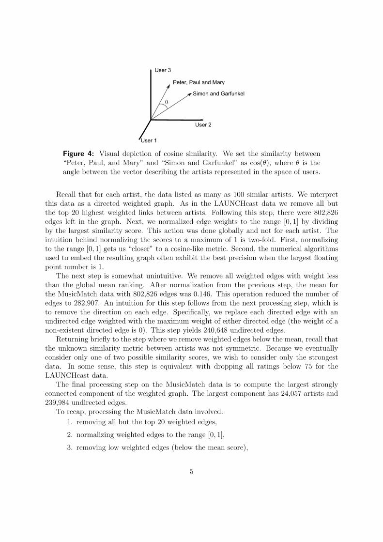
Figure 4: Visual depiction of cosine similarity. We set the similarity between“Peter, Paul, and Mary” and “Simon and Garfunkel” as cos(θ), where θ is theangle between the vector describing the artists represented in the space of users.

Recall that for each artist, the data listed as many as 100 similar artists. We interpretthis data as a directed weighted graph. As in the LAUNCHcast data we remove all butthe top 20 highest weighted links between artists. Following this step, there were 802,826edges left in the graph. Next, we normalized edge weights to the range [0, 1] by dividingby the largest similarity score. This action was done globally and not for each artist. Theintuition behind normalizing the scores to a maximum of 1 is two-fold. First, normalizingto the range [0, 1] gets us “closer” to a cosine-like metric. Second, the numerical algorithmsused to embed the resulting graph often exhibit the best precision when the largest floatingpoint number is 1.

The next step is somewhat unintuitive. We remove all weighted edges with weight lessthan the global mean ranking. After normalization from the previous step, the mean forthe MusicMatch data with 802,826 edges was 0.146. This operation reduced the number ofedges to 282,907. An intuition for this step follows from the next processing step, which isto remove the direction on each edge. Specifically, we replace each directed edge with anundirected edge weighted with the maximum weight of either directed edge (the weight of anon-existent directed edge is 0). This step yields 240,648 undirected edges.

Returning briefly to the step where we remove weighted edges below the mean, recall thatthe unknown similarity metric between artists was not symmetric. Because we eventuallyconsider only one of two possible similarity scores, we wish to consider only the strongestdata. In some sense, this step is equivalent with dropping all ratings below 75 for theLAUNCHcast data.

The final processing step on the MusicMatch data is to compute the largest stronglyconnected component of the weighted graph. The largest component has 24,057 artists and239,984 undirected edges.

To recap, processing the MusicMatch data involved:

1. removing all but the top 20 weighted edges,

2. normalizing weighted edges to the range [0, 1],

3. removing low weighted edges (below the mean score),

5

Symb. Meaning

A the weighted adjacency matrixδij the Kronecker deltae a column vector of onesE set of edges

(i, j) an edge between vertex i and jL the Laplacian matrixn the number of verticesU layout energyV set of verticesxi the position of vertex i embedded in R

1

Xik the kth coordinate of vertex i embedded in Rd

wij weight on edge (i, j)

Table 1: The notation used in this paper.

4. symmetrizing each edge by taking the maximum weight of each directed edge, and

5. computing the largest connected component of the resulting graph.

Unlike the LAUNCHcast data, we did do some parameter tuning to determine whatcut-off parameter to use in step 3. Other parameters (including removing step 3) yieldedsubjectively worse results. In actuality, knowledge of the underlying similarity metric or rawrankings would allow us to further tune this processing.

4 Graph Embeddings

Given a weighted undirected graph G = (V, E, w), one way to visualize this graph is to assigncoordinates to every node. This process is called embedding the graph. We want a set oflow-dimensional coordinates that illuminate internal properties of the data. In particular,for our data we would like “similar” artists to be placed “nearby” each other in embedding.This problem is common and many solutions exist [12, 2, 11]. As we will show, our solutionsare related to the previous work, but we prefer an alternative derivation to highlight theassumptions implicit in the optimization problem.

To describe our embeddings, we first write both a single and multi-dimensional quadraticenergy function and then discuss the problems with this function. The next two sub-sectionsdescribe two different “fixes” for these problems. Finally, we provide a section with explicitformulas for the resulting optimization problems in three-dimensions to make our ideasconcrete.

This section is greatly expanded in the Appendix, where we discuss motivation for theseembeddings. Also, we further elaborate on alternatives to the embeddings which yield poorresults.

6

4.1 One-Dimensional Quadratic Energy

One possibility to embed the graph is a weighted quadratic term over the edges of the graph.Intuitively, this idea gives rise to a quadratic “energy” that “attracts” nodes connected withedges. If we restrict ourselves to a one-dimensional embedding and label all the vertices withintegers from 1 to n, we have a coordinate xi ∈ R

1 for each vertex i ∈ V . For convenience,we represent the set of all coordinates in a length n vector x. Given an embedding x, thenthe “energy” of the embedding is

U(x) =∑

(i,j)∈E

wij(xi − xj)2 = (1/2)

∑

ij

Aij(xi − xj)2

=∑

ij

Lijxixj,(1)

where A is the weighted symmetric adjacency matrix (Aij = Aji = wij) and L is the Laplacianmatrix,

Lij = δij

∑

k

Aik − Aij.

In matrix notation, we have that

L = Diag(Ae) − A and U(x) = xT Lx,

where e is the vector of all ones.Although the quadratic energy function has significant problems that we will address

soon, we first wish to write the multi-dimensional generalization. Let Xik be the kth coor-dinate of the embedding of vertex i into R

d and let X represent the n × d matrix of all thecoordinates. The quadratic energy of embedding X is

U(X) =∑

(i,j)∈E

d∑

k=1

(Xik − Xjk)2 =

∑

ij

d∑

k=1

LijXikXjk

= trace(XT LX).

(2)

To discuss the problems with these embeddings, we return to one-dimensional embeddingsfor simplicity. The problems we describe remain for the multi-dimensional function as well.

Ideally, we would like to embed a graph by minimizing U(x), that is, embed the graphwith x∗ where

x∗ = argminx U(x).

However, this optimization problem has a simple minimizer, x∗

i = 0. Needless to say, theembedding of a graph to a single point is not good.

The function U has two properties that cause this behavior. First, the minimizer of Uis not unique. If x is a minimizer of U(x), then for any scalar γ, x + γ is also a minimizer.Second, for any scalar γ < 1, then U(γx) = γU(x) < U(x). By the second property, xi = 0for all i is a minimizer and therefore xi = γ for any scalar is also a minimum.

7

Two solution to these problems which lead to better graph embedding are discussed inthe next two sections. The key idea in each solution is to add a set of constraints to theoptimization problem to restrict the possible solutions x∗.

4.2 Spectral Embedding

One set of constraints that yields a non-trivial solution results in the following optimizationproblem

minX

U(X)

s.t.∑

i Xik = 0 for 1 ≤ k ≤ d∑

i XikXil = nδkl for 1 ≤ k ≤ l ≤ d.

(3)

In matrix notation, we havemin

Xtrace(XT LX)

s.t. XT e = 0XT X = nId,

where Id is the d × d identity matrix.We interpret these constraints as follows. The constraint

∑

i Xik = 0 fixes the center ofthe resulting embedding at the origin. In light of the problems discussed at the end of theprevious section, this constraint removes the problem of finding non-unique minimizers byadding scalars. Next, taking k = l the constraint

∑

i X2ik = n fixes Xik 6= 0 for at least one

vertex i in each coordinate k and prevents the minimizer from collapsing to the origin.When k 6= l, the constraint

∑

i XikXil = 0 enforces orthogonality. The implication of thisconstraint is that the resulting embedding must use all d dimensions available. To understandwhy this aspect is important, notice that the objective function, equation (2), is independentbetween dimensions. This constraint correlates the solution X between dimensions. Howeverthis constraint also implies that the solution in dimension k + 1 has a higher energy thandimension k.

In fact, the solution to equation (3) is known analytically. The minimizing matrix Xis composed of the eigenvectors of L corresponding to the second through d + 1th smallesteigenvalues. In fact, in one-dimension, the solution of this optimization problem gives theFiedler vector of the graph [5]. In higher dimensions, this embedding is well studied undermany different names [2].

4.3 Spherical Embedding

Another set of constraints that yields a non-trivial embedding gives the optimization problem

minX

U(X)

s.t.∑

i Xik = 0 for 1 ≤ k ≤ d∑d

k=1 X2ik = 1 for 1 ≤ i ≤ n.

(4)

8

In matrix notation, the problem is

minX

trace(XT LX)

s.t. XT e = 0diag(XXT ) = e.

As in the previous problem, the constraint∑

i Xik = 0 implies that the center of the

embedding is at the origin. The constraint,∑d

k=1 X2ik = 1, however, fixes each point on

the surface of a d-dimensional hyper-sphere. A result of this constraint is that the resultingembedding cannot collapse to the origin.

The cost of this second constraint is that there is no longer an analytical solution to theembedding problem. Instead, we must employ non-linear numerical optimization proceduresto compute the embedding X that minimizes equation (4). A second consequence of thisconstraint is that the embedding problem is intractable in one-dimension. The surface of aone-dimensional hyper-sphere is simply the set of points {1,−1}. Thus, in one-dimension,this constraint yields an integer optimization problem.

The earliest reference (of which we are aware) to the idea of spherical mapping is fromAntonio and Metzger in their work on mapping processes to a hypercube multi-processorconfiguration [1]. Further, this same optimization problem results from examining low-ranksolutions to the semi-definite program (SDP) in Goemans and Williamson’s approximationalgorithm for the minimum bisection problem [4, 7]. Recently, others have used SDP methodsfor low-dimensional embeddings [14].

4.4 Embeddings in Three-Dimensions

In the previous sections, we wrote the optimization problems for each of the embeddingsfor an arbitrarily high dimension. While this approach illuminates some of the analyticalrelationships between the method, it may hide some details. In this section, we restrictourselves to three-dimensions and explicitly write the optimization programs.

For this section, let xi, yi and zi represent the first, second, and third coordinates of theembedding point for vertex i. The spectral embedding optimization problem is

minx,y,z

∑

ij Lijxixj + Lijyiyj +∑

ij Lijzizj

s.t.∑

i xi = 0∑

i yi = 0∑

i zi = 0∑

i x2i = n

∑

i y2i = n

∑

i z2i = n

∑

i xiyi = 0∑

i xizi = 0∑

i yizi = 0.

(5)

As previously mentioned, the solution to this optimization problem is to set x, y and z tobe the eigenvector corresponding to the second, third, and fourth smallest eigenvalues of L,respectively.

The spherical embedding problem in 3d is

minx,y,z

∑

ij Lijxixj + Lijyiyj +∑

ij Lijzizj

s.t.∑

i xi = 0∑

i yi = 0∑

i zi = 0x2

i + y2i + z2

i = 1 for all i.

(6)

9

(a) Geodesic Grid

(b) Robinson (c) Sinusoidal (d) Equidistant Azimuthal

Figure 5: In this figure, we plot a series of different map projections. We beginwith a simple geodesic (latitude/longitude) layout. Figures (b)-(d) show threedifferent projects each preserving some visual aspect of the geodesic lines. Figure(b) actually draws a slight perturbation of the geodesic grid to better representthe behavior of the projection near the hemisphere edges.

The solution of this problem is a set of coordinates on the unit sphere. Also, to reiterate,there is no known analytical solution to this problem and it must be solved by a numericaloptimization routine.

5 Map Projections

At the end of the last section, we determined two methods to embed the graph. Jumpingahead to the results, the most useful embedding is the spherical embedding. In order to usethe spherical projections to compute a two-dimensional layout, however, we must computeplanar points from locations on the surface of the sphere.

This problem has been studied for over 2,000 years under a different name: drawing amap [13, 3]. The map drawing community produced a plethora of techniques to draw theEarth on a flat map. The large number of techniques exists because there is no perfectmap drawing. Loosely speaking, the three types of distortion are area, length, and angles.An area preserving map is called an equal area projection, a length preserving map is anequidistant projection, and an angle preserving map is a conformal projection.

10

After surveying a large number of map projections using Matlab’s Mapping Toolbox [10],we decided to investigate three projections, Robinson, sinusoidal, and equidistant azimuthal.Figure 5 displays the result of each of these projections on the geodesic grid. We report onsome properties of each projection below. None of the projections we choose are conformal.For our application, this property is not important.

Robinson The Robinson projection preserves no property. It distorts area, length, andangles. Instead of a mathematical formula, the Robinson projection is a set of heuristicsto construct an appealing map drawing. The National Geographic Society has used theRobinson projection since 1988 for its world map [3].

Sinusoidal The sinusoidal projection, also known as the Sanson-Flamsteed projection, isan equal area projection. At the poles, the projection collapses to a point.

Equidistant Azimuthal The equidistant azimuthal projection is an equidistant projec-tion. The projection unrolls the near hemisphere into a circle such that distances are pre-served near the center of the projection. The far hemisphere is highly distorted.

6 Implementation

We used a combination of off-the-shelf and custom software in this project. The implemen-tation is divided into many scripts that accomplish one part of the data processing pipeline.This approach allowed us the flexibility of choosing different languages for many of the dif-ferent steps. Largely speaking, the implementation nicely divides between preprocessing,embedding, and visualization. Our implementation and processing scale to datasets withmillions of artists.1

Preprocessing Our preprocessing scripts were written in Matlab, Perl, and C++. We firstused custom Perl scripts to convert the raw datafiles provided by Yahoo!’s music services intoa sparse matrix representation. For the LAUNCHcast data, we performed the filtering andsimilarity graph construction using two C++ programs. The program to build the similaritygraph used the routine CLUTO_V_GetGraph from CLUTO [8]. Preprocessing the MusicMatchdata was done entirely in Matlab.

Embedding To compute the spectral embeddings, we used the eigs routine in Matlab.For the spherical embedding, we took advantage of the relationship with a low-rank semi-definite program and used the SDP-LR software to compute these embeddings [4]. To unrollthe spherical embedding into a planar set of points, we used the routines eqdazim, sinusoid,

1While the computation and visualization tools scale to this level, their utility for such a large dataset be-comes questionable. For a dataset with one million points, the points are almost completely dense throughoutthe sphere and we tend to observe less interesting clustering behavior.

11

and robinson from the Matlab Mapping Toolbox [10]. We manually picked the center ofeach projection.

Visualization tools We used two custom built visualization tools for this experiment:plot3d, and visgraph. We have used both programs on graphs with over 100,000 vertices andone million edges.

First, we use plot3d to investigate the structure of the three-dimensional spectral andspherical embeddings. The plot3d program takes an edge list and a set of coordinates asinput, and optionally, a clustering partition for coloring the nodes. It is a C++ programthat uses OpenGL to draw each node and each edge. Users interactively rotate and zoomthe embeddings of the graph to gain a perspective on the embedding quality. It includesspecial code for the spherical embedding to draw a reference sphere at the center.

Once we determine that an embedding is worth pursing, we unroll the three-dimensionalspherical points into two dimensions and use the visgraph program to interactively browse atwo-dimensional graph layout. Like plot3d, visgraph takes similar input, but can also accepta set of labels for each node in the graph. The nodes (points) and the edges (lines) arealpha-blended to show local density. The program maintains a quad-tree data structure toallow fast label browsing using a circular “brushing cursor” to reveal labels. This techniqueavoids cluttering the display with all labels simultaneously. Figure 8 demonstrates examplesof the visualizations from visgraph.

Publication Tools For publication images, we use a set of perl scripts to convert rawembedding data into POVRAY files for further rendering. Also, the visgraph program hasan option to save the current drawing as an SVG file. Both POVRAY and SVG files areresolution independent formats which make them ideal for generating high quality still imagesof the datasets.

7 Results and Discussion

Figure 9-13 present the main results of the paper. In figures 9 and 10, we compare theembeddings computed by equation (6) and equation (5), respectively. Figures 12 and 13show the LAUNCHcast and MusicMatch datasets for each of the map projections describedin section 5. Throughout the rest of this section, we will use these figures to argue thatthe spherical embeddings are superior to the spectral embeddings, and that the Robinsonprojection yields the “best-looking” map projection for our data.

First, the two spherical embedding figures show each of the artists represented as a singlepoint on the surface of the sphere. The color of each point identifies the cluster an artistbelongs to from an independent clustering of each similarity graph using CLUTO [8]. Thespherical embeddings show a nice grouping of points of similar color, which indicates thatthe coordinates for the points largely agree with the clustering. Thus, these embeddingsare successful and we are representing “similar” artists “nearby” each other. In the twospectral embedding figures, the results are less clear. Here, we have drawn the artists using

12

the same colors. While the LAUNCHcast spectral embedding shows a reasonable separationbetween groups of artists, the MusicMatch spectral embedding yields one large heterogeneous“clump” of artists. In fact, for both LAUNCHcast and MusicMatch, the spherical embeddingdisplays a larger number of small dense “clusters” of artists than the spectral embeddings.The failure of the eigenvectors of the Laplacian to yield a good embedding may be relatedto the power-law structure in the data as was observed by Lang [9].

We have omitted the comparisons in two-dimensions due to space constraints becausethe results are uniformly worse for the spectral embedding. Briefly, the LAUNCHcast imageshows only the approximately ± 45 degree “arms” of the clustering. The MusicMatch imageshows a large mess of points at the origin.

We use the CLUTO clustering for two purposes: first, to evaluate the results, and second,to improve the visualization. CLUTO is a high-quality clustering program with thousandsof successful experiments. In this case we use CLUTO to generate a set of 50 clusters foreach of the similarity graphs.

Next, we will address the map projections. Figures 12 and 13 show each of the mapprojections from the display used in visgraph. Each artist is a point colored according tothe artist’s cluster from CLUTO. All edges longer than distance 2 for LAUNCHcast and 3for MusicMatch are not drawn — many of these long edges would have “wrapped around”the other side of the sphere. Each edge is drawn with a low alpha-blending value (alpha =0.025) so “brighter” regions represent higher edge density.

The distortion at the edges in the latitude/ longitude drawing are extreme and visuallyunappealing for both graphs. The severe distortion at the edge of the sinusoidal projection isalso unappealing. Both of these projections either expand (latitude/longitude) or compress(sinusoidal) important groups of points. Subjectively, the Robinson projection looks mostappealing and removes the most severe expansion from the latitude/longitude projectionwhile maintaining the a nice expansive layout. Finally, the equidistant azimuthal projectiondisplays the near hemisphere (the center of the picture) with a nice separation, but the farhemisphere is overly distorted into a circular shape.

8 Exploration

In this section, we describe our explorations of the “World of Music.” All of the visualizationsuse the Robinson projection. We do not explain all of the insight we have gained from thesevisualizations, only a few succinct points that highlight the utility of the visualization.

LAUNCHCast We have explored the LAUNCHcast data extensively. In this section,we note three interesting features. First, in the middle of one of the empty areas (“theoceans”), there is a single artist. Second, there is a strong relationship between “indie”music and “mainstream” music, belying the independence of “indie” music. Third, there isa group of “bridge” artists between “mainstream” music and “techno” music.

The artist in the middle of the “ocean” is Austin Powers. Although attributing a causeto the placement of a particular artist is difficult, we can form some hypotheses. If Austin

13

Powers is an artist, then their position in the layout has been affected by the numerouserrant rankings placed on them in reference to Austin Powers, the movie.2 Instead, if AustinPowers refers to the movie, the position may be influence by the non-standard use of themovie title as the musical artist name. Either way, it indicates an outlier in the data thatmerits further attention.

Second, we plotted the locations of a few well-known “indie” musical artists, The Shins,Death Cab for Cutie, and The Decemberists, along with the location of more well known“mainstream” musical artists, U2, Soundgarden, Courtney Love, and Stereophonics. Thevisualization shows that the group of “indie” artists forms a tight cluster near the moreextended cluster of mainstream artists. Together, the “indie” and “mainstream” artistsform the region that looks like North America in the center of the Robinson projection.While alternate specific analysis would have revealed this result, the visualization makes itimmediate.

Finally, the visualization shows a set of “bridge” artists. These artists form a smallcluster between “mainstream” music and “techno” music. Bridge artists, and particularlya group of bridge artists, are important sets of musical artists because they relate multipleclusters.3 Again, the visualization immediately highlights this group due to the pattern ofedges entering and existing.

MusicMatch While browsing through the MusicMatch data, we found many interestingclusters and artists. In this section, we highlight a few of our observations. First, we founda cluster of Latter Day Saints musicians. Second, we found a few interesting artists that“connect” various group. Finally, there is a cluster of children’s musicians. See figure 7 forsupporting visualizations from the visgraph tool.

The Latter Day Saints (LDS) cluster is interesting from a few perspectives. Becauseof the uniform color of all the artists, CLUTO identified this grouping of artists as well.However, finding this group by browsing the CLUTO clusters is onerous. We asked CLUTOfor 50 clusters, which it happily provided. Determining the semantics behind these clusters,however, is beyond CLUTO and requires human intervention. Globally, the LDS clusterstands out in the visualization due to its unique shape. The shape invites further investiga-tion. Further, once someone sees the artist “Church of Jesus Christ of Latter Day Saints,”he or she can easily hypothesize and confirm the nature of the cluster. This process is moreengaging and fulfilling than a brute-force human evaluation of all 50 clusters.

Second, while browsing around the graph, some artists stand out with a “connector”pattern. Typically, these artists have multiple (3-4) dense sets of edges emanating from asingle point. Visually, these artists break from the regularity of the surrounding region. Inparticular, Will Downing is an “connector” artist between soul, R&B, and jazz. Producersmay like such artists because they influence multiple sets of other artists; consumers maylike such artists because they help expand musical tastes.

2Previously, we were under the impression that Austin Powers was indeed an artist unrelated to themovie. However, recent searches to confirm this fact have not been successful.

3We write more on the importance of connector artists below.

14

(a) Austin Powers in the middle of nowhere.

(b) Indie music is closely related to mainstream music.

(c) The bridge from mainstream to techno music.

Figure 6: Some exploration results from the LAUNCHcast dataset.

15

Finally, we have highlighted a set of children’s musicians. While the particular artistsare fairly well known and contain little important information, the surrounding region andthe connections are rich with data that should interest musical producers and marketers.Unfortunately, without expertise in the domain, we cannot evaluate this region ourselves.However, the visual presentation of the material is key to identifying the possibility of ex-tracting this data. Without the visual presentation, it would not have occurred to us to seekmore information about children’s musicians and their relationships to the other musicians.

9 Related Work

[Note: this section is incomplete and lacks appropriate references.]The major contribution of this paper are a more detailed exposition of the techniques

used in [6] as well as demonstrating that the techniques continue to work on another datasetas well. To reiterate, we view a data exploration problem as a dimensionality reduction andgraph embedding problem. From each of these viewpoints, there exists significant literature.

One of the standard methods for graph embedding is multi-dimensional scaling (MDS).This method is not as computationally scalable as our approach. In order to make MDStechniques effective, they must include a repulsive force which includes a computational costof n log n (for a fast multipole/quad tree appraoch) or n2 (for an exact computation) periteration. Our procedure does not include a repulsive force and has a linear cost per iteration.Instead, it relies on the constraints of the optimization problem for “sufficient repulsion.”To be clear, there is no reason to believe the constraints in the hyper-sphere optimizationproblem will lead to anything like a repulsive force, but for the music graphs, the final effectis a nice cluster separation and hence, “sufficient repulsion.”

The MDS approach is strongly related to a force-directed layout. Computed an embed-ding of the similarity graph using the yEd graph layout tool. As exhibited in figure 11, theresults are inferior to the embeddings computed with our tools.

10 Future Work

There are a few aspects of this project that merit further investigation. First, the layout of theunrolled maps needs to be hand tuned to determine a good origin and rotation of the sphere.While conceptually simple, this problem has a strong combinatorial aspect which makesstraightforward optimization techniques difficult. Using a grid search based approach wouldbe a significant step toward automating this step. Second, the current approach is to projectthe points on the surface of the sphere to a two-dimensional plane. A useful alternative maybe to directly visualize the sphere and avoid the projection to two-dimensions. Finally, thisapproach works for large datasets (more than 250,000 nodes), but the resulting embeddingsare nearly useless due to the density of points throughout the sphere. To be clear, thereis structure present in the embedding, but a direct visualization seems of limited use. Ourbelief is that a two-dimensional space is too restrictive and we need visualization techniques

16

(a) The cluster of Latter Day Saints musicians.

(b) An artist that “connects” a set of clusters

(c) The cluster of children’s musicians.

Figure 7: Some exploration results from the MusicMatch dataset.

17

for higher dimensional point sets.

11 Conclusions

In this paper, we built a world of music based on ratings from users. We used two datasetsderived from user ratings to compute a similarity graph between musical artists. To embedthe graph, we examined two embeddings based on quadratic energy functions. Empirically,we found the spherical embedding to be superior to the spectral embedding. To computea set of planar points from the spherical embedding, we considered three map projections,of which the Robinson was the most appealing. By combining these embeddings with a setof visualization tools, we developed a system to interactively browse the underlying datasetand help build an understanding for the world of music.

12 Acknowledgments

Todd Beaupre deserves special acknowledgment for giving us the LAUNCHCast dataset andspending his time explaining the data and what Yahoo! Music would like to understandabout the data. Chris Staszak provided the MusicMatch dataset.

References

[1] John K. Antonio and Richard C. Metzger. Hypersphere mapper: a nonlinear program-ming approach to the hypercube embedding problem. J. Parallel Distrib. Comput.,19(3):262–270, 1993.

[2] Mikhail Belkin and Partha Niyogi. Laplacian Eigenmaps for Dimensionality Reductionand Data Representation. Neural Comp., 15(6):1373–1396, 2003.

[3] Lev M. Bugayevskiy and John P. Synder. Map Projections: A Reference Manual. Taylorand Francis, 1995.

[4] Samuel Burer and Renato D.C. Monteiro. A nonlinear programming algorithm forsolving semidefinite programs via low-rank factorization. Mathematical Programming(series B), 95(2):329–357, 2003.

[5] Miroslav Fiedler. Algebraic connectivity of graphs. Czech. Math J., 23:298–305, 1973.

[6] David Gleich, Kevin Lang, Matt Rasmussen, and Leonid Zhukov. The world of music:Sdp embedding of high-dimensional data. In Information Visualization, Minneapolis,Minnesota, 2005. Interactive Poster.

18

(a) visgraph showing labels on LAUNCHcast. (b) visgraph showing zoomed edge on Music-Match.

Figure 8: visgraph usage shots.

[7] Michel X. Goemans and David P. Williamson. Improved Approximation Algorithms forMaximum Cut and Satisfiability Problems Using Semidefinite Programming. J. Assoc.Comput. Mach., 42:1115–1145, 1995.

[8] George Karypis. Cluto – a clustering toolkit. Technical Report 02-017, University ofMinnesota, Department of Computer Science, 2002.

[9] Kevin Lang. Fixing two weaknesses of the spectral method. In Advances in NeuralInformation Processing Systems, 2005.

[10] MathWorks. Matlab mapping toolbox: Version 2.0.2, May 2004.

[11] J. C. Platt. Fast embedding of sparse music similarity graphs. In Advances in NeuralInformation Processing Systems, volume 16, pages 571–578, 2004.

[12] Sam T. Roweis and Lawrence K. Saul. Nonlinear dimensionality reduction by locallylinear embedding. Science, 290(5500):2323–2626, December 2000.

[13] John P. Snyder. Flattening the Earth: Two Thousand Years of Map Projections. Uni-versity of Chicago Press, 1993.

[14] Kilian Q. Weinberger and Lawrence K. Saul. Unsupervised learning of image mani-folds by semidefinite programming. In Proceedings of the 2004 IEEE Computer SocietyConference on Computer Vision and Pattern Recognition, 2004.

[15] Brian Whitman and Steve Lawrence. Similiarty for music from community metadata.In International Computer Music Conference, pages 591–598, Goeteborg, Sweden, Sep-tember 2002.

19

(a) LAUNCHcast (b) MusicMatch

Figure 9: Spherical embeddings of the similarity graph from both datasets displayed as point-clouds.

20

(a) LAUNCHcast (b) MusicMatch

Figure 10: Spectral embeddings of the similarity graph from both datasets displayed as point-clouds. Thesepictures represent 3d point clouds. For the MusicMatch picture, this figure excludes a few points that wereoutside the dense point-cloud near the origin.

21

Figure 11: A force directed layout of the LAUNCHcast similarity graph using theyEd graph editor and layout program. We exported the layout from yEd and usedvisgraph to generate the image above. As in the other pictures, the colors comefrom the CLUTO clustering. This image shows that the force-directed approachused in yEd is not able to separate the clusters like the energy-minimizationapproach we use.

22

(a) Latitude/Longitude (b) Robinson

(c) Sinusoidal (d) Equidistant Azimuthal

Figure 12: Map projections of the LAUNCHcast spherical embedding.

23

(a) Latitude/Longitude (b) Robinson

(c) Sinusoidal (d) Equidistant Azimuthal

Figure 13: Map projections of the MusicMatch spherical embedding.

24

A Quadratic Energy Embeddings

As we stated in section 4, one way to visualize an undirected graph G = (V, E, w) is to assigncoordinates to every node. This process is called embedding the graph. Ideally, we want aset of low-dimensional (ideally two-dimensional) coordinates with properties “like:”

• for each edge (i, j) ∈ E, vertex i and vertex j should be “close” in the embedding,

• for vertex pairs (i, j) /∈ E with a large number of edges on the shortest path betweenvertex i and vertex j, the vertices should be “far” in the embedding, and

• the embedding “reveals” non-trivial information about the graph.

We indicate these terms with scare-quotes to emphasize that these are not (yet) rigorousmathematical properties of the embeddings. Instead, these are subjective evaluation metricswe can use to compare and contrast different embeddings of the same data.

If we restrict ourselves to a one-dimensional embedding and label all the vertices withintegers from 1 to n, we have a coordinate xi ∈ R

1 for each vertex i ∈ V . For convenience,we use the vector x to represent the set of all coordinates. Throughout this paper andin particular throughout this appendix, we will look at quadratic energy embeddings. Aquadratic energy embedding is a quadratic difference term over the edges of the graph.

In the quadratic energy formula, each edge e = (i, j) contributes “energy”

wij(xi − xj).

This term has the effect of pulling nodes connected with edges close because the minimum ofthis term is when xi = xj. For the entire graph G, the quadratic “energy” of the embeddingis

UG(x) =∑

(i,j)∈E

wij(xi − xj)2. (7)

We call this function an “energy” because of the relationship with the energy of a mass-springsystem. Section ?? elaborates on this relationship.

An alternative graph embedding is to use a set of springs on the edges of the graph. For alinear spring with constant k, the potential energy stored in the spring with scalar extensionx is

U(x) =1

2kx2.

In our case, we have kij = wij and x = (xi−xj). This expression is why we call our quadraticenergy embedding an “energy” embedding, if each edge is a spring, then we minimize thetotal potential energy in the system given by UG(x).

25